Constrained Markov Decision Processes with Application to Wireless Communications

Alexander Zadorojniy

Constrained Markov Decision Processes with Application to Wireless Communications

Final Paper

Submitted in Partial Fulfillment of the

Requirements for the Degree of

Master of Science in

Electrical Engineering

Alexander Zadorojniy

Submitted to the Senate of the Technion – Israel Institute of Technology

SIVAN , 5764 HAIFA June 2004

The Final Paper Was Done Under

The Supervision of Professor A. Shwartz

in the Faculty of Electrical Engineering

I Would Like To Express My Deep Gratitude

To Professor A. Shwartz

For His Guidance and Help

Throughout All Stages of the Research.

THE GENEROUS FINANCIAL SUPPORT OF TECHNION IS GRATEFULLY ACKNOWLEDGED.

Contents

Page

Abstract…………………………………………………………………………...…..1

List of Symbols and Notations……...……………………..………………………....2

1. Introduction…………………………………………..……………………..…....4

2. Survey and Research Objectives………..…………..……………………...……5

3. Wireless Communications System Model………..……………………………..7

4. Constrained Markov Decision Processes (CMDP) and Linear Programming

Approach………………...………………………………………………..…..…10

4.1 CMDP……..……………………………………………………………….…10

4.2 Optimal Policies for CMDP Problem……….……………………………..…12

4.3 Occupation Measure and Linear Programming (LP)……...…………………13

5. The Optimal Policy Properties for CMDP……………...………………..……18

5.1 The Karush-Kuhn-Tucker (KKT) Conditions…………………………..……18

5.2 The Fundamental Theorems………………………………..…………..…….22

6. The Optimal Policy Properties for Power Saving Problem……………….….29

6.1 CMDPS Algorithm for Two Control Levels..………………………..………35

6.1.1 CMDPS Algorithm…………………………….……………...……...37

6.1.2 CMDPS Algorithm Usage…………..………………………………..39

6.1.3 Example of CMDPS Algorithm Application to CMDPS Problems....45

6.2 CMDPS Algorithm for Finite Number of Control Levels…………….……..50

Contents ( Cont. )

Page

7. A New Approach to Optimization of Wireless Communications…...……….55

7.1 Communications Problem Optimization Using CMDP Approach….……….58

7.2 CMDPS Algorithm Application in Wireless Communications……...………62

8. Conclusions and Further Research…………………………………..…….….66

Appendix A: Linear Programming (LP) and Simplex Method Idea………….…67

Appendix B: Principle of Optimality and Value Iteration Algorithm........…..…73

Appendix C: BPSK Modulation in Fading Environment………………..…….…75

References………………………………………..……………………………….…77

Hebrew Abstract………………………………………………………………...……I

List of Figures

Number Page 1. Wireless Communications System Model…………… ……………………….…8

2. Markov Chain for Monotonicity Proof………………………………………..…30

3. Coupled System……………………………..…...……………………………….30

4. Randomization Changes…………………...………………………………..……36

5. CMDPS Algorithm Diagram…………………...………………...………………40

6. Markov Chain for Example 1…………………………………………………….46

7. The Simplex Method Results………………………….…………………………51

8. Randomization Behavior in Example 1…………………..…………………..…..52

9. Markov Chain of the Wireless Communications Problem…..…………….……..56

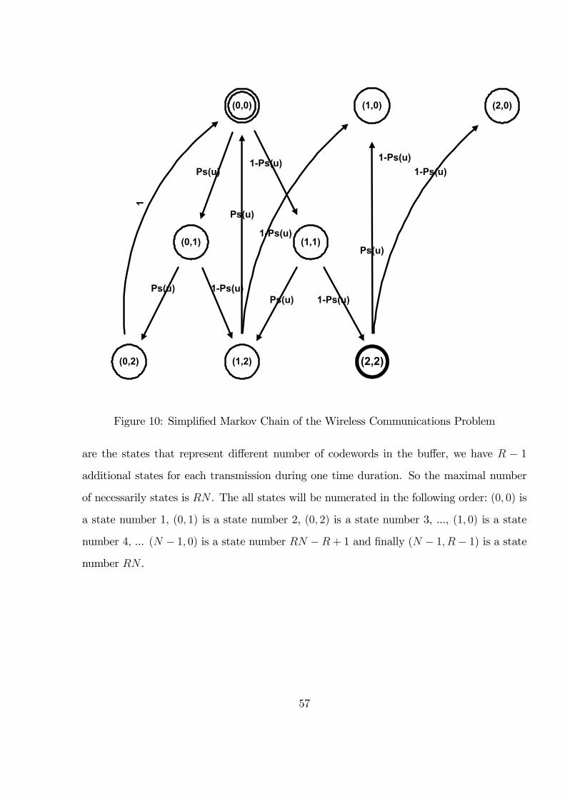
10. Simplified Markov Chain of the Wireless Communications Problem ………..…57

11. Markov Chain for Communications Problem Example…………………….……63

12. Geometric Solution…………….…………………………………………..…….69

13. Simplex Method – Geometric Motivation………………………………...……..70

Abstract

With the development of personal communication services, portable terminals such as mobile

telephones and notebook computers are expected to be used more frequently and for longer

times. Hence power consumption will become even more important than it is now. One of

the major concerns in supporting such mobile applications is the energy conservation and

managements in mobile devices. In wireless communications, low power may cause errors

during the transmission. Therefore when we try to conserve power we have to care about

the Quality-of-Service.

In recent years several solution methods were introduced. Usually these methods find

the optimal power policy for minimal average delay under average power constraint. Some

of them are for continuous time domain and other for discrete one. Methods which solve the

problem in the continuous time domain are general but they are not always applicable for

digital systems, and these type of systems are most popular in recent years. Methods which

deal with discrete time domain, in many cases, are not general enough, only for two control

levels, for example. As usual, in digital systems we are interested to find an optimal policy

which minimizes the average delay under average and peak power constraints and uses only

available discrete power levels. None of the existing methods can give us this capability.

This research deals with a derivation of new solution methods for constrained Markov

decision processes and applications of these methods to the optimization of wireless com-

munications. We intend to survey the existing methods of control, which involve control of

power and delay, and investigate their effectiveness. We introduce a new type of power con-

trol in wireless communications, which minimizes the transmission delay under the average

power constraint where at each slot uses one of the available discrete power levels, while the

maximal power level is limited by a peak power constraint. Moreover we develop algorithm

which, aside from the optimization problem solving, will be able to show sensitivity of the

solution to changes in the average power level constraint.

1

List of Symbols and Notations

ACK The acknowledge about successful transmission

NACK The acknowledge about failure

SNR The signal to noise ratio

AWGN The additive white Gaussian noise

MDP Markov decision processes

CMDP Constrained Markov decision processes

CMDPS Algorithm Constrained Markov decision processes solver algorithm

KKT Conditions Karush- Kuhn Tucker Conditions

N The buffer size

rk The random variable that represents a fading at slot k

nk The random variable that represents an AWGN at slot k

lk The codeword transmitted at slot k

yk The received word at slot k

R The transmission rate

λ The arrival rate

4t The slot duration

π A policy

σ The initial state

X The state space

U The action space

P (u) = {Pij(u)} The transition matrix when action u ∈ U is taken

c = c(x, u) The immediate cost at state x ∈ X using action u ∈ U

C = C(σ;π) The value of the criterion when starting at σ and using policy π

2

d = d(x, u) The immediate cost, related to the constraint

D = D(σ;π) The value of the constraint criterion

ρ(x, u) The probability to be at state x ∈ X and use action u ∈ U

β The discount factor

µx(u) The ratio of using action u ∈ U at x ∈ X to all possible actions

α The average available power

z A vector of length n

b A vector of length m

s A vector of variables of length n

A An m× n matrix

Eb A transmitted signal energy per bit

Tb A time duration of one bit transmission

fc A carrier frequency

3

1 Introduction

In this paper we consider a situation where one type of cost (delay, throughput,etc...) is to

be minimized while keeping the other types of costs (power, delay, etc.) below some given

bounds. Posed in this way, our control problem can be viewed as a constrained optimization

problem over a given class of policies.

Telecommunications networks are designed to enable the simultaneous transmission of

different types of traffic: voice, file transfers, interactive messages, video, etc. Typical per-

formance measure are the transmission delay, power consumption, throughput, transmission

error probabilities, etc. Different types of traffic differ from each other by their statistical

properties, as well by their performance requirements. For example, for interactive messages

it is necessary that the average end-to-end delay be limited. Strict delay constraints are

important for voice traffic; there, we impose a delay limit of 0.1 second. When the delay

increases beyond this limit, it becomes quickly intolerable. For non-interactive file transfer,

we often wish to minimize delays or to maximize throughput.

A trade-off exists between achieving a small delay, on the one hand, and low power

consumption on the other. Note that delay minimization and conserving power are two

conflicting performance metrics. To minimize the delay we should transmit with the highest

possible power because it will increase the probability of successful transmission and decrease

the number of retransmissions. On the contrary, to decrease power consumption, we are

interested to transmit with lowest possible power. The problem is formulated as a constrained

MDP, where we wish to minimize the costs related to the delay subject to constraints on the

average and peak power.

4

2 Survey and Research Objectives

We can divide the known work in the subject of saving energy to two types: first, the

energy conservation control problem by assuming there is a finite supply of information to

be transmitted and second, where the supply of information to be transmitted is infinite.

The first type of problems are considered in [12]. In this work the authors analyze the

power control problem in transferring a finite-size data under a total energy constraint as

well as delay constraints. In the paper they considered a problem with only two power levels:

a constant power or zero power (i.e., no transmission). A randomized power control scheme

is discussed, i.e., the transmitter can select either power level with a certain probability. The

power control problem is (given the total energy and the file size) to find the optimal policy

that maximizes the probability of success under either an average delay constraint or a strict

delay constraint. These two problems form a constrained Markov decision problem and they

can be solved via a dynamic programming algorithm. In order to solve them the authors

used the techniques which were developed in [1] and [8].

The second type of problems are considered in ([5], Chapter 7.4). In this problem the

author assumes that there exists a buffer so that the information rate into it is constant and

a transmission rate is constant as well. The cost function is defined as buffer size at time

k plus power, that was used in this time, multiplied by a Lagrange multiplier in order to

control the average power. This optimization problem was solved by dynamic programming

algorithm [4]. More precisely, the optimal equation was derived by dynamic programming

techniques, and the equation itself was solved by the value iteration method (Appendix B),

[4] and [8].

The first work helps us to better understand the optimal policy for problems with average

and peak constraints for two control levels but the solution for general problem when we

have constraints for both peak and average power (or delay) simultaneously, with finite, but

arbitrary number of control levels is still unclear from this paper. The second one is much

more general. When the author is solving the optimization problem he takes care of average

5

power by Lagrangian multiplier so that the average power will be below some chosen level.

The problem is that when the level of average power is given and we need to find the suitable

Lagrangian multiplier - this can be a not trivial mathematical problem. In the paper the

author shows what is a necessarily power levels in order to get an optimal solution, but it

is not clear what happens if this power level is not available, in other words, if we have

discrete levels of power and need to find the optimal solution by using only these power

levels. The more complicated question can be asked as well, what happens to optimal policy

when the level of average available power is changing. Or another question, if the policy will

be changed in the same way when we have a small change in the average available power

and when we have a big change in it. Or what is the behavior of the optimal solution for

this kind of problems. Or does there exist common properties of the solution for different

values of average power level constraints.

One way to solve the first two problems is, instead of using the value iteration method

for optimality equation, to represent the problem in the linear programming form [1] and

to solve it by the simplex method [3] and (Appendix A). In order to answer the rest of the

questions we will derive and prove theorems and based on them algorithm that will solve the

problem (sections 5,6). Moreover the optimal solution that is derived from the new developed

algorithm will be compared to the solution obtained from the simplex method (section 6).

We will show that in addition to the ability of the solution sensitivity investigation, the

algorithm can be used as a tool for solving constrained Markov decision processes problems

(sections 5,6). In section 7 the algorithm will be used in order to solve a wireless optimization

problem that will be defined in section 3.

In this research we developed two fundamental theorems (section 5.2) which describe the

structure of the optimal solution for general constrained Markov decision process problems.

Two additional theorems, that describe the properties of the solution for constrained Markov

decision process in power saving problems, were developed in section 6. In section 6.1.1 we

developed innovative algorithm which solves constrained Markov decision process for power

saving problems and which was applied to wireless communications problems in section 7.2.

6

3 Wireless Communications System Model

Our system model can be represented by five blocks (Figure 1): buffer, transmitter, fading

channel, receiver and controller.

A buffer is a device that receives codewords with rate λ, stores and removes them de-

pending on "Buffer Control" value.

A transmitter is a device that transmits codewords with rate R and power u which

depends on the "Power Control" value.

A fading Channel is a channel where except for additive noise, there exists multiplicative

disturbances that impact the amplitude of the transmitted signal.

A receiver is a device that receives the transmitted signal, decodes it, if needed, and

transmits acknowledge (ACK or NACK) to the Controller in the transmitter side.

A controller is a device that has one input and two outputs. The input to the controller

is a feedback from the receiver. The first output, named "Buffer Control", controls when the

codewords are removed from the buffer or stored in it. The second output, named "Power

Control", controls the power level that the transmitter should use.

This system works as follows: the transmitter transmits codewords from the buffer,

afterward an amplitude of the transmitted signal is multiplied by disturbances and additive

noise is added to it. In order to write a precise expression for this process, let’s define the

following:

Definitions:

• rk is a random variable that represents a fading at slot k.

• nk is a random variable that represents an additive white Gaussian noise (AWGN ) at

slot k.

• lk is a codeword transmitted at slot k.

• yk is a received word at slot k.

7

Buffer Transmitter ReceiverFadingChannel

Controller Power ControlBuffer Control

Feedback Channel for Success(ACK)/Failure(NACK)

λ R

Figure 1: Wireless Communications System Model

• R is a transmission rate. It is constant over the whole period of transmission.

• λ is an arrival rate. It is constant over the whole period of transmission.

• 4t is the slot duration.

• ACK is an acknowledge about successful transmission.

• NACK is an acknowledge about failure.

In Communications the relationship between transmitted codeword and received code-

word can be expressed by the following formula [7]

yk = rklk + nk (1)

Now we will describe a block fading Gaussian channel model:

• This model assumes that the fading-gain process is constant on blocks of N symbols.

• It is modeled as a sequence of independent random variables, each of which is the

fading gain in a block.

• Except a fading there exists an additive white Gaussian noise (AWGN ), where thefading and AWGN are iid and independent from each other.

8

We assume a block fading Gaussian channel in which the fading of each slot is iid ac-

cording to some distribution (such as Rayleigh, Rice etc...). At each slot a codeword is

transmitted with constant rate R[codewords/time duration]. The information rate into the

buffer is constant λ[codewords/time duration].

Define

4t , 1

R[codewords]

Transmission power is constant during each slot 4t and may vary between slots. We assume

that the average power of AWGN and fading disturbances remain at the same level during

the whole period of the transmission.

If a transmission succeeds an ACK is returned to the controller in the transmitter side

using a feedback channel without errors and delay. Otherwise a NACK is returned through

the feedback channel without errors and delay, causing a retransmission of the data until

an ACK is returned. The buffer stores the information that has to be transmitted. The

information is removed from the buffer only if an ACK is returned. We assume that the

buffer size is large enough so that we can neglect any loss of information due to overflow. We

aim at finding the value of the optimal transmission power at each slot so that the average

delay is minimal, the average power is below a given level α, and at each slot one of the

available discrete power levels is used where maximal power level is limited by a peak power

constraint. The important thing to notice is that at each slot only one codeword can be

transmitted.

We will try to represent this model as Constrained Markov Decision Process (CMDP)

model.

Let us now introduce CMDP and the new algorithm that will help us to optimize the

solution of the communications problem. We will return to the communications problem in

section (7).

9

4 ConstrainedMarkov Decision Processes (CMDP) and

Linear Programming Approach

Markov decision processes (MDP), also known as controlled Markov chains, constitute a

basic framework for dynamically controlling systems that evolve in a stochastic way. We

focus on discrete time models: we observe the system at times t = 1, 2, ..., n where n is

called horizon, and may be either finite or infinite. A controller has an influence on both

the costs and the evolution of the system, by choosing at each time unit some parameters,

called actions. As is often the case in control theory, we assume that the behavior of the

system at each time is determined by what is called the ’state’ of the system, as well as the

control action. The system moves sequentially between different states in a random way; the

current state and control action fully determine the probability to move to any given state

in the next time unit.

MDP is thus a generalization of (non-controlled) Markov chains, and many useful prop-

erties of Markov chains carry over to controlled Markov chains. A key Markovian property

is that conditioned on the state and action at some time t, the past states and the next one

are independent.

The model that we consider in this paper is special in that more than one objective cost

exists; the controller minimizes one of the objectives subject to constraints on the other. We

will call this class of MDP Constrained MDP, or simply CMDP.

4.1 CMDP

Definition: A finite constrained Markov decision process is a 7-tuple {X,U, P, c, C, d,D} [1]

and [6] , where

• X is the state space that contains a finite number of states.

• U is the finite set of actions.

10

• P (u) = {Pij(u)} is the transition matrix when action u is taken.

• c = c(x, u) is the immediate cost at state x using action u.

• C = C(σ;π) is the value of the criterion when starting at σ and using policy π.

• d = d(x, u) =

d1

d2

.

.

dn

is a vector of immediate costs, related to constraints, when at

state x and using action u.

• D = D(σ;π) is the vector of values of the constraint criteria when starting at σ and

using policy π.

• ≥ for vectors means that each elements in the left hand vector is greater or equal tothe corresponding element in the right hand one.

• Similar definitions hold for ≤ and =.

We now define the cost criteria. For any policy π and initial distribution σ at t = 1, the

finite horizon cost for a horizon n is defined as [1]

Cn(σ, π) =nXt=1

Eπσc(Xt, Ut)

An alternative cost that gives less importance to the far future is the discounted cost.

For a fixed discount factor β, 0 < β < 1, define

Cnβ (σ, π) = (1− β)

nXt=1

βt−1Eπσc(Xt, Ut)

Cβ(σ, π) = limn→∞

Cnβ (σ, π)

11

Since there are finitely many states and actions, the lim indeed exists as a limit and

Cβ(σ, π) = (1− β)∞Xt=1

βt−1Eπσc(Xt, Ut)

Also, in a similar way we derive for the discounted cost, that is related to constraint, that

Dβ(σ, π) = (1− β)∞Xt=1

βt−1Eπσd(Xt, Ut) (2)

Quite frequently, the discounted cost is defined without the normalizing constant (1−β).The techniques are the same for both cases, we can get one from another by multiplying

or dividing the immediate cost by this factor. There are several advantages of using this

normalization. First, we avoid the situation where, for fixed immediate cost c, the total

discounted cost becomes very large if β is close to one. Second, with this normalization,

the discounted cost will be seen to converge to the expected average cost when stationary

policies are used. Finally, we shall see that the LP used to solve the discounted and the

expected average costs has the same form when the normalization constant is used.

For a fixed real vector V , we define the constrained control problem COP as:

Find a policy that minimizes Cβ(σ, π) subject to Dβ(σ, π) ≤ V .

4.2 Optimal Policies for CMDP Problem

Optimal policies are defined with respect to a given initial state. A policy that is optimal

for one state might not even be feasible for another. In fact, there may be some initial states

at which no policy is feasible, where feasible policy is a policy that satisfies the constraints.

This is in contrast to non-constrained MDPs, in which there typically exist policies that are

optimal for all initial states.

The class of Markov policies turns out to be rich in the following sense. For any policy,

the exists an equivalent Markov policy that induces the same marginal probability measure,

12

i.e., the same probability distribution of the pairs (Xt, Ut), t = 1, 2, ... [1]

All cost criteria that we defined in the previous subsection have the property that they are

functions of the distribution of these pairs. We conclude that Markov policies are sufficiently

rich so that a cost that can be achieved by an arbitrary policy can also be achieved by a

Markov policy. Moreover the Markov policies are dominating for any cost criterion which is

a function of the marginal distribution of states and actions ([1], Theorem 2.1).

4.3 Occupation Measure and Linear Programming (LP)

An occupation measure corresponding to a policy π is the total expected discounted time

spent in different state-action pairs. It is thus a probability measure over the set of state-

action pairs and it has the property that the discounted cost corresponding to that policy

can be expressed as the expectation of the immediate cost with respect to this measure.

More precisely, define for any initial distribution σ, any policy π and any pair x, u:

fβ(σ, π;x, u)def= (1− β)

∞Xt=1

βt−1P πσ (Xt = x,Ut = u), x ∈ X,u ∈ U(x)

fβ(σ, π) is then defined to be the set {fβ(σ, π;x, u)}x,u. It can be considered as a proba-

bility measure, which we call the occupation measure, that assigns probability fβ(σ, π;x, u)

to the pair (x, u).

13

The discounted cost can be expressed as [1]

Cβ(σ, π) = (1− β)Eπσ{

∞Xt=1

βt−1c(xt, ut)}

= (1− β)∞Xt=1

βt−1Eπσc(xt, ut)

= (1− β)∞Xt=1

Xx,u

βt−1P πσ (xt = x, ut = u)c(x, u)

=Xx,u

(1− β)∞Xt=1

βt−1P πσ (xt = x, ut = u)c(x, u)

=Xx,u

(1− β)∞Xt=1

βt−1P πσ (xt = x, ut = u)c(x, u)

=Xx,u

fβ(σ, π;x, u)c(x, u)

Cβ(σ, π) =Xx∈X

Xu∈U

fβ(σ, π;x, u)c(x, u) (3)

Also, in a similar way we derive for the discounted cost, related to the constraint, that

Dβ(σ, π) =Xx∈X

Xu∈U

fβ(σ, π;x, u)d(x, u) (4)

Lemma ([10])

Xy∈X

Xu∈U(y)

fβ(σ, π; y, u)(δx(y)− βPyx(u)) = (1− β)σ(x), ∀x ∈ X (5)

fβ(σ, π; y, u) ≥ 0, ∀y, u (6)Xy∈X

Xu∈U(y)

fβ(σ, π; y, u) = 1 (7)

Proof:

If x 6= σ then P πσ (Xt=1 = x,Ut=1 = u) = 0 so that

14

Xu∈U(x)

fβ(σ, π;x, u) =X

u∈U(x)(1− β)

∞Xt=1

βt−1P πσ (Xt = x, Ut = u)

=X

u∈U(x)(1− β)

∞Xt=2

βt−1P πσ (Xt = x, Ut = u)

= (1− β)∞Xt=2

Xu∈U(x)

βt−1P πσ (Xt = x, Ut = u)

= (1− β)β∞Xt=1

Xu∈U(x)

βt−1P πσ (Xt+1 = x,Ut+1 = u)

= (1− β)β∞Xt=1

Xy∈X

Xu∈U(y)

βt−1P πσ (Xt = y, Ut = u)Pyx(u)

= βXy∈X

Xu∈U(y)

(1− β)∞Xt=1

βt−1P πσ (Xt = y, Ut = u)Pyx(u)

= βXy∈X

Xu∈U(y)

fβ(σ, π; y, u)Pyx(u)

Thus Xu∈U(x)

fβ(σ, π;x, u) = βXy∈X

Xu∈U(y)

fβ(σ, π; y, u)Pyx(u), for x 6= σ (8)

If x = σ then, in the first equality above we have an additional term

(1− β)P πσ (Xt=1 = x, Ut=1 = u) = (1− β)

Therefore for x = σ we can rewrite (8) as

Xu∈U(x)

fβ(σ, π;x, u) = βXy∈X

Xu∈U(y)

fβ(σ, π; y, u)Pyx(u) + (1− β) (9)

From (5) we can see that for x 6= σ (5) equals to (8) and for x = σ (5) equals to (9). (6)

and (7) is established from the definition of fβ(σ, π; y, u). Therefore the proof is completed.

¥

15

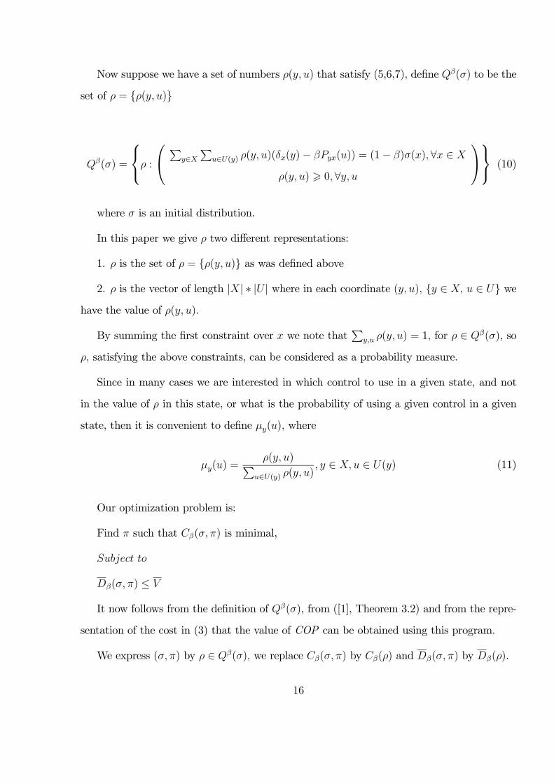
Now suppose we have a set of numbers ρ(y, u) that satisfy (5,6,7), define Qβ(σ) to be the

set of ρ = {ρ(y, u)}

Qβ(σ) =

ρ :

Py∈X

Pu∈U(y) ρ(y, u)(δx(y)− βPyx(u)) = (1− β)σ(x),∀x ∈ X

ρ(y, u) > 0,∀y, u

(10)

where σ is an initial distribution.

In this paper we give ρ two different representations:

1. ρ is the set of ρ = {ρ(y, u)} as was defined above

2. ρ is the vector of length |X| ∗ |U | where in each coordinate (y, u), {y ∈ X, u ∈ U} wehave the value of ρ(y, u).

By summing the first constraint over x we note thatP

y,u ρ(y, u) = 1, for ρ ∈ Qβ(σ), so

ρ, satisfying the above constraints, can be considered as a probability measure.

Since in many cases we are interested in which control to use in a given state, and not

in the value of ρ in this state, or what is the probability of using a given control in a given

state, then it is convenient to define µy(u), where

µy(u) =ρ(y, u)P

u∈U(y) ρ(y, u), y ∈ X, u ∈ U(y) (11)

Our optimization problem is:

Find π such that Cβ(σ, π) is minimal,

Subject to

Dβ(σ, π) ≤ V

It now follows from the definition of Qβ(σ), from ([1], Theorem 3.2) and from the repre-

sentation of the cost in (3) that the value of COP can be obtained using this program.

We express (σ, π) by ρ ∈ Qβ(σ), we replace Cβ(σ, π) by Cβ(ρ) and Dβ(σ, π) by Dβ(ρ).

16

So we can rewrite this program as a linear program (LP) as follows

LP β1 (σ) : Find ρ such that Cβ(ρ) =

Px,u c(x, u)ρ(x, u) is minimal,

Subject to

Dβ(ρ) =P

x,u d(x, u)ρ(x, u) ≤ V

ρ ∈ Qβ(σ) .

The last constraint is linear by definition (10).

So we can derive the following theorem ([1], Theorem 3.3)

Equivalence between COP and the LP

Theorem ([1], Theorem 3.3): Consider a finite CMDP, then

• For any fβ(σ, µ) there exists ρ ∈ Qβ(σ) such that ρ = fβ(σ, µ), and conversely for any

ρ ∈ Qβ(σ) there exists µ such that ρ = fβ(σ, µ).

• LP β1 (σ) is feasible if and only if COP is. Assume that COP is feasible. Then there

exists an optimal solution ρ∗ for LP β1 (σ), and the stationary policy µ, that is related

to ρ∗ through (11), is optimal for COP.

17

5 The Optimal Policy Properties for CMDP

In this chapter we will derive a number of theorems that describe important properties of

CMDP problems solutions. The most valuable theorems are based on Karush-Kuhn Tucker

conditions and prove in a very elegant way a statement that looks intuitive but not trivial

for formal proof. We begin with considering a problem with two control levels and one

constraint and extend it to arbitrary, but finite, number of control levels and one constraint.

5.1 The Karush-Kuhn-Tucker (KKT) Conditions

Definitions:

• z is a vector of length n.

• b is a vector of length m.

• s is a vector of variables of length n.

• A is an m× n matrix.

• · denotes a scalar product.

Consider the following linear programming problem.

Minimize z · s (12)

Subject to A · s ≥ b (13)

s ≥ 0 (14)

The Karush-Kuhn-Tucker (KKT) conditions can be stated as follows:

There exist w and v so that

18

A · s ≥ b, s ≥ 0 (15)

w ·A+ v = z, w ≥ 0, v ≥ 0 (16)

w · (A · s− b) = 0, v · s = 0 (17)

The first condition (15) merely states that the candidate point must be feasible; that is,

it must satisfy the constraints of the problem. This is usually referred to as primal feasibility.

The second condition (16) is usually referred to as dual feasibility, since it corresponds to

a feasibility of the problem closely related to the original one. Here w and v are called the

Lagrangian multipliers (or dual variables) corresponding to the constraints A · s ≥ b and

s ≥ 0 respectively.

Finally, the third condition (17) is usually referred to as complementary slackness.

Theorem ([3], KKT Conditions, inequality case):

Any solution s that satisfies conditions (15)-(17) is an optimal solution of the Linear

Programming problem (12)-(14).

Consider the following linear programming problem with equality constraints.

Minimize z · s (18)

Subject to A · s = b (19)

s ≥ 0 (20)

19

By changing the equality into two inequalities of the form A · s ≥ b and −A · s ≥ −b,the KKT conditions developed earlier would simplify to

A · s = b, s ≥ 0 (21)

w ·A+ v = z, w unrestricted, v ≥ 0 (22)

v · s = 0 (23)

Theorem ([3], KKT Conditions, equality case):

Any solution s that satisfies conditions (21)-(23) is an optimal solution of the Linear

Programming problem (18)-(20).

For linear programming problems, these conditions are both necessary and sufficient and

hence form an important characterization of optimality.

The main difference between these conditions for the inequality problem is that the

Lagrangian multiplier vector (or dual vector) w corresponding to the constraint A · s = b is

unrestricted in sign.

The major objective of this paper is to solve a communications problem (section 3), for

which, as we will see later, only equality conditions are requiered. Therefore in this section

we will derive general theorems for equality case only.

Now let’s represent our optimization problem (LP β1 (σ)) in the form described by (21)-

(23).

Definitions:

• z is a vector of length n = |X| ∗ |U |, this is a vector of the cost, which we represent asa row vector.

20

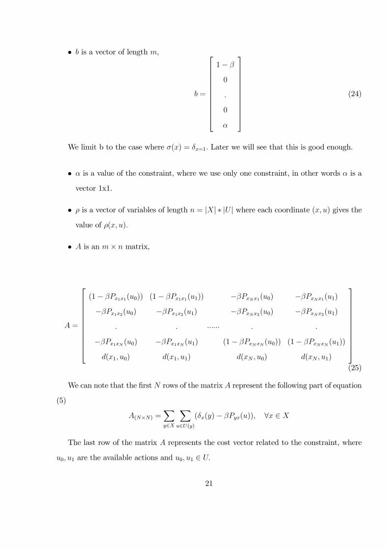
• b is a vector of length m,

b =

1− β

0

.

0

α

(24)

We limit b to the case where σ(x) = δx=1. Later we will see that this is good enough.

• α is a value of the constraint, where we use only one constraint, in other words α is a

vector 1x1.

• ρ is a vector of variables of length n = |X| ∗ |U | where each coordinate (x, u) gives thevalue of ρ(x, u).

• A is an m× n matrix,

A =

(1− βPx1x1(u0)) (1− βPx1x1(u1))

−βPx1x2(u0) −βPx1x2(u1)

. .

−βPx1xN (u0) −βPx1xN (u1)

d(x1, u0) d(x1, u1)

......

−βPxNx1(u0) −βPxNx1(u1)

−βPxNx2(u0) −βPxNx2(u1)

. .

(1− βPxNxN (u0)) (1− βPxNxN (u1))

d(xN , u0) d(xN , u1)

(25)

We can note that the first N rows of the matrix A represent the following part of equation

(5)

A(N×N) =Xy∈X

Xu∈U(y)

(δx(y)− βPyx(u)), ∀x ∈ X

The last row of the matrix A represents the cost vector related to the constraint, where

u0, u1 are the available actions and u0, u1 ∈ U.

21

So by using (5-7) and definitions of z, b, α, ρ,A,Cβ(σ, π) we can rewrite (18) - (20) as

Minimize z · ρ (26)

Subject to A · ρ = b (27)

ρ ≥ 0 (28)

and (21)-(23) as

A · ρ = b, ρ ≥ 0 (29)

w ·A+ v = z, w unrestricted, v ≥ 0 (30)

v · ρ = 0 (31)

5.2 The Fundamental Theorems

Now we will derive the fundamental theorems. These theorems describe the structure of the

optimal solution for constrained Markov decision process problems and are used as a basis

for innovative algorithm that will be derived later.

In order to derive our new theorems we will use ([1], Theorem 3.8).

Theorem ([1], Theorem 3.8) (Bounds on the number of randomizations)

If the constrained optimization problem is feasible then there exists an optimal stationary

policy π such that the total number of randomizations that it uses is at most the number of

constraints.

Let X0 and X1 be disjoint sets of states so that |X0|+ |X1| = N − 1. Let xi be the onlystate not in X0 ∪X1. Let

πq(x) =

δu0, x ∈ X0

δu1, x ∈ X1

(1− q)δu0 + qδu1, x = xi

(32)

22

Fix α0 so that COP is feasible. By theorem ([1], Theorem 3.8), πqα0 is optimal, where

πqα0 is randomized only in state xi, and α0 = D(σ, πqα0 ).

Definitions:

• u0, u1 ∈ U.

• 0 ≤ qα0 ≤ 1.

• αmin = inf0≤q≤1

D(σ, πq).

• αmax = sup0≤q≤1

D(σ, πq).

• πqα is the policy that is the same as πqα0 except in state xi and πqα is chosen so that the

value of the constraint is α, where αmin ≤ α ≤ αmax. This is possible because D(σ, πqα)

is continuous in qα. The continuity will be proven later.

• α = D(σ, πqα), αmin ≤ α ≤ αmax.

Lemma 1: D(σ, πqα) is continuous in qα.

From Lemma 1 we can conclude that ∀ αmin ≤ α ≤ αmax, ∃ 0 ≤ qα ≤ 1 s.t. D(σ, πqα) = α.

Proof. Dβ(σ, πqα) = (1− β)

P∞t=1 β

t−1Eπqασ d(Xt, Ut)

Given ε, fix N s.t.

(1− β)P∞

t=N βt−1maxX,U |d(Xt, Ut)| < ε4

⇒ ¯̄Dβ(σ, π

qα)−Dβ(σ, πqα+δ)

¯̄ ≤ ε2+

+¯̄̄(1− β)

PN−1t=1 βt−1Eπqα

σ d(Xt, Ut)− (1− β)PN−1

t=1 βt−1Eπqα+δ

σ d(Xt, Ut)¯̄̄.¯̄̄

(1− β)PN−1

t=1 βt−1Eπqασ d(Xt, Ut)− (1− β)

PN−1t=1 βt−1Eπqα+δ

σ d(Xt, Ut)¯̄̄=

|(1− β)PN−1

t=1

Px∈X

Pu∈U β

t−1P tσ,x(π

qα)d(x, πqα(x))−(1− β)

PN−1t=1

Px∈X

Pu∈U β

t−1P tσ,x(π

qα+δ)d(x, πqα+δ(x))|where P t

yx(πq) = P t−1

yx (πq)[(1− q)P (π0) + qP (π1)].

Thus, the expression¯̄̄(1− β)

PN−1t=1 βt−1Eπqα

σ d(Xt, Ut)− (1− β)PN−1

t=1 βt−1Eπqα+δ

σ d(Xt, Ut)¯̄̄

23

we can represent as a¯̄̄(1− β)

PN−1t=1 βt−1poly(t, qα)− (1− β)

PN−1t=1 βt−1poly(t, qα + δ)

¯̄̄,

where poly(t, q) is a polynom in q, of order t.

Since this is a finite sum we can choose δ so that¯̄̄(1− β)

PN−1t=1 βt−1poly(t, qα)− (1− β)

PN−1t=1 βt−1poly(t, qα + δ)

¯̄̄< ε

2

therefore¯̄Dβ(σ, π

qα)−Dβ(σ, πqα+δ)

¯̄< ε. So ∀ε > 0, ∃δ > 0

so that¯̄Dβ(σ, π

qα)−Dβ(σ, πqα+δ)

¯̄< ε therefore we proved the Lemma.

With a some abuse of notation we will use πqα0 instead of πqα0 (x).

Theorem 1 Consider a constrained Markov decision process problem with two control levels

and one constraint, where 0 < qα0 < 1. Then for each αmin ≤ α ≤ αmax, πqα is an optimal

policy.

Proof. The proof will be done by KKT conditions.

For convenience let us rearrange the states so thatX0 = {x1, ..., xi−1}, X1 = {xi+1, ..., xN}.

Since randomization is allowed only in state xi then under πqα0 for any xj 6= xi there

exists at most one u so that ρ(xj, u) 6= 0. Moreover, if ρ(xi, u) = 0 under πqα0 , then this istrue also under any πqα , αmin ≤ α ≤ αmax.

From the ([1], Theorem 3.8) πqα0 is optimal so KKT conditions are satisfied for πqα0 .

Denote the Lagrange multipliers by vπqα0 , wπqα0 for πqα0 , and vπ

qα, wπqα for πqα .

Arrange the elements of ρπqα0 = ρ(πqα0 ) = fβ(σ, π

qα0 ) as

ρπqα0 = (ρ(x1, u0), ρ(x1, u1), ..., ρ(xi, u0), ρ(xi, u1), ..., ρ(xN , u0), ρ(xN , u1))

= (ρ(x1, u0), 0, ..., ρ(xi−1, u0), 0, ρ(xi, u0), ρ(xi, u1), 0, ρ(xi+1, u1), ..., 0, ρ(xN , u1))

From (31) < vπqα0 , ρπ

qα0 >= 0. Because ρ(xi, u0) > 0 and ρ(xi, u1) > 0, then v0i = 0 and

v1i = 0, and v = 0 in all coordinates where ρ(x, u) > 0, so

vπqα0 = (0, v11, ..., 0, v

1i−1, 0, 0, v

0i+1, 0, ..., v

0N , 0)

24

Let’s check KKT conditions (29-31) for policy πqα .

Since changing qα does not change the structure, except perhaps to create more "0", it

follows that ρπqα= fβ(σ, π

qα) takes the form

ρπqα= (ρ0(x1, u0), 0, ..., ρ0(xi−1, u0), 0, ρ0(xi, u0), ρ0(xi, u1), 0, ρ0(xi+1, u1), ..., 0, ρ0(xN , u1))

(33)

We choose wπqα = wπqα0 and vπqα= vπ

qα0

Equation (29) is satisfied because ρπqα is a feasible solution by definition.

Equation (30) is satisfied because wπqα = wπqα0 and vπqα= vπ

qα0 , and A and z are the

same for each choice of α.

Equation (31) is satisfied because for vπqα= vπ

qα0 it doesn’t matter what is a ratio be-

tween µxi(u0) and µxi(u1), and because ∀m 6= i µπα

xm(u0) = µπqα0

xm (u0) (µπα

xm(u1) = µπqα0

xm (u1)),

therefore

< vπqα, ρπ

qα>=< vπ

qα0 , ρπqα0 >= 0

Now we will extend this theorem from two control levels to an arbitrary, but finite,

number of control levels.

Fix α0 so that COP is feasible. By theorem ([1], Theorem 3.8), πqα0 is optimal, where

πqα0 is randomized only in state xi, and α0 = D(σ, πqα0 ).

Definitions:

• u0, u1, ..., us ∈ U.

• Let X0, X1, ...,Xs be disjoint sets of states so that |X0| + |X1| + ... + |Xs| = N − 1.

25

Let xi be the only state not in X0 ∪X1 ∪ ... ∪Xs. Let

πqα0 (x) =

δu0 , x ∈ X0

δu1 , x ∈ X1

.

.

.

δus , x ∈ XsPi q

iα0δui , x = xi

• 0 ≤ qjα0 ≤ 1,∀i or in another representation 0 ≤ qα0 ≤ 1.

• Pj qjα0= 1, and at most two qjα0 > 0.

• αmin = infqα0

D(σ, πqα0 ) s.t. the same two qjα0 as above are non zero.

• αmax = supqα0

D(σ, πqα0 ) s.t. the same two qjα0 as above are non zero.

• πqα is the policy that is the same as πqα0 except in state xi and πqα is chosen so that

the value of the constraint is α, where αmin ≤ α ≤ αmax, and zeros of qα are also zeros

of qα0 . This is possible because α, α ∈ [αmin, αmax], is continuous in qα. The continuitywill be proven later.

• α = D(σ, πqα).

Lemma 2: D(σ, πqα) is continuous in qα.

Proof. The proof is similar to the proof of Lemma 1.

From Lemma 2 we can conclude that ∀ αmin ≤ α ≤ αmax, ∃ 0 ≤ qα ≤ 1 where zeros ofqα are also zeros of qα0 ,

Pj q

jα = 1 s.t. D(σ, π

qα) = α.

Theorem 2 Consider a constrained Markov decision process problem with arbitrary, but

finite, number of control levels and one constraint, where 0 < qα0 < 1. Then for each

αmin ≤ α ≤ αmax, πqα is an optimal policy.

26

Proof. The proof will be done by KKT conditions.

For convenience let us rearrange the states so that X0 = {x1, ..., xj}, ...,

Xr = {xk, ..., xi−1}, .., Xs = {xs, ..., xN}.

Since randomization is allowed only in state xi then for any xj 6= xi there exists at most

one u so that ρ(xj, u) 6= 0.

From the ([1], Theorem 3.8) πqα0 is optimal so KKT conditions are satisfied for πqα0 .

Denote the Lagrange multipliers by vπqα0 , wπ

qα0 for πqα0 , and vπqα , wπqα for πqα .

Arrange the elements of ρπqα0 = ρ(πqα0 ) = fβ(σ, π

qα0 ) as

ρπqα0 = (ρ(x1, u0), ρ(x1, u1), ..., ρ(x1, us), ..., ρ(xi, up), ..., ρ(xi, uj), ..., ρ(xN , us−1), ρ(xN , us))

= (ρ(x1, u0), 0, ..., 0, ..., ρ(xi, up), 0, ..., 0, ρ(xi, uj), ..., 0, ρ(xN , us))

From (31) < vπqα0 , ρπ

qα0 >= 0. Because ρ(xi, up) > 0, ρ(xi, uj) > 0 then vpi = 0, vji = 0

and v = 0 in all coordinates where ρ(x, u) > 0. Thus,

vπqα0 = (0, v11, ..., v

s1, ..., 0, 0, ..., v

s−1N , 0)

Let’s check KKT conditions (29-31) for policy πqα.

Since changing qα does not change the structure, except perhaps to create more "0", it

follows ρπqα = fβ(σ, π

qα) takes the form

ρπqα= (ρ0(x1, u0), 0, ..., 0, ..., ρ0(xi, up), 0, ..., 0, ρ0(xi, uj), ..., 0, ρ0(xN , us)) (34)

We choose wπqα = wπqα0 and vπ

qα = vπqα0

Equation (29) is satisfied because ρπqα is a feasible solution by definition.

Equation (30) is satisfied because wπqα = wπqα0 and vπ

qα = vπqα0 , and A and z are the

same for each choice of α.

27

Equation (31) is satisfied because for vπqα = vπ

qα0 it doesn’t matter what is a ratio

between µxi(up) and µxi(uj), and ∀m 6= i µπqα

xm (up) = µπqα0

xm (up), and αmin and αmax are

obtained without changing actions therefore

< vπqα, ρπ

qα>=< vπ

qα0 , ρπqα0 >= 0

28

6 The Optimal Policy Properties for Power Saving Prob-

lem

Now we will extend our analysis to the power saving problem. We start with a two control

levels problem and one constraint, and will extend it to arbitrary, but finite, number of

control levels. Let define u0 and u1 as power control levels, where u0 < u1.

Assumption 1: For each α for which there exists a feasible solution, there exists a

unique optimal solution.

Assumption 2 (monotonicity assumption): For strictly increasing value of the ratioµxi(u1)

µxi(u0), the value of the constraint α is strictly increasing, where α ∈ [αmin, αmax] and xi is

the state with randomization.

In the problem defined by diagram on Figure 2 we will show analytically that Assumption

2 is satisfied.

Let’s consider the problem: ∀xj, where 0 ≤ j < i the transmission is by u1, ∀xj, wherei < j ≤ N the transmission is by u0, at xi we have randomization between u0 and u1.

The transitions are allowed between neighborhood states only, where the state is defined as

the number of messages in the buffer. Define two systems (Figure 3) where in system 1,

P (u = u1|x = xi) = κ and in system 2, P (u = u1|x = xi) = κ0 where κ0 > κ. So we can

say that ratioµxi(u1)

µxi(u0)at system 2 is higher than at system 1. Using a coupling, we assume

that at any time t, a success in system 1 implies a success in system 2. Two systems have

the same buffer and channel. Server 1 transmits with u = u1 in xi with probability κ and

server 2 transmits with u = u1 in xi with probability κ0. Assume that P (success|u = u1) >

P (success|u = u0) > 0.5.

Lemma 3 Consider the two systems as described in Figure 2 and 3. The average power

usage at the second system is higher than at the first one, where average power this is the

value of the constraint α.

Proof. Till we are not at state xi, the power usage in both systems is the same, because

29

X(i-1) Xi

Ps(u)

X(i+1)

Ps(u0) Ps(u0)Ps(u1)

1-Ps(u1)1-Ps(u1) 1-Ps(u) 1-Ps(u0)

Figure 2: Markov Chain for Monotonicity Proof

Server 1

Server 2

Buffer

Buffer

Channel

Channel

Figure 3: Coupled System

30

except state xi systems are same. When we arrive to state xi we have three possibilities for

systems behaviors:

1). No one of the transmissions in both servers is successful, so the two systems continue

to be the same.

2). Both systems have succeeded, so the two systems continue to be the same.

3). First system failed to transmit but the second succeeded to transmit.

Note, the two systems are initially at the same state, so the first time that 3) can happen,

is when both systems are at state xi.

Until 3) happens we have two equal systems. So let’s concentrate on the third case.

If 3) has happened, at system 2 we always transmit with power u1 till again we will

arrive to state xi, and at system 1 we always transmit with power u0 till again we will arrive

to state xi. Let’s denote the period of time that both systems are in different states by τ .

During the period of time τ the power usage at the second system is higher that at the first

one and when this time is finished both system always meet at the same state (from diagram

2 we can see that τ can finished only at states x0 or xN). So after time τ > 0 both systems

again at the same state and such we begin the same procedure from the beginning.

Because an average power usage is equal to the sum of all instantaneous power usages

divided by a period of measured time then we can conclude that the average power usage at

the second system is higher than at the first one as we required to prove.

For more complicates Markov chains we will show numerically that Assumption 2 is

satisfied (section 7).

Fix απqk so that COP is feasible. By theorem ([1], Theorem 3.8), πqk is optimal, where πqk

is randomized only in state xi, and απqk = D(σ, πqk).

Definitions:

• k is a number of states where µy(u1) = 1 (µy(u0) = 0).

31

• Let X10 and X1

1 be disjoint sets of states so that |X10 | = N − 1− k, and |X1

1 | = k. Let

xi(k) be the only state not in X10 ∪X1

1 , where i(k) denotes index i as function of k.

πq1k (x) =

δu0 , x ∈ X1

0

δu1 , x ∈ X11

(1− q1)δu0 + q1δu1 , x = xi(k)

• Let X2

0 and X21 be disjoint sets of states so that |X2

0 | = N − 2− k, and |X21 | = k + 1.

Let xi(k+1) be the only state not in X20 ∪X2

1 , where xi(k+1) 6= xi(k), X10 = {X2

0 , xi(k+1)},X21 = {X1

1 , xi(k)}.

ςq2k+1(x) =

δu0 , x ∈ X2

0

δu1 , x ∈ X21

(1− q2)δu0 + q2δu1 , x = xi(k+1)

Note, for q2 = 0 and q1 = 1, ς

q2k+1(x) is equal to π

q1k (x).

• Let X30 and X3

1 be disjoint sets of states so that |X30 | = N − 1− j, and |X3

1 | = j. Let

xr be the only state not in X30 ∪X3

1 .

ξq3j (x) =

δu0, x ∈ X3

0

δu1, x ∈ X31

(1− q3)δu0 + q3δu1 , x = xr(j)

(35)

• α = supq1

D(σ, πq1k ) and α = infq1

D(σ, πq1k ).

In the following two theorems we are talking about range of α for which a feasible solution

exists.

32

Theorem 3 Consider a finite CMDP so that Assumptions 1 and 2 are satisfied. If policy

πq1k is optimal for some απq1k ≤ α then there exists some ας

q2k+1 > α so that ςq2k+1 is optimal

for αςq2k+1.

Proof. The proof will be done by contradiction.

By Theorem 1 πq1k is optimal for α ≤ απq1k ≤ α. From Monotonicity (Assumption 2), πq1k

is optimal for α = α when q1 = 1.

Assume that ςq2k+1 is not the optimal solution of the problem for any αi such that αςq2k+1 ≥

αi > α, where αςq2k+1 this is a number so that u1 ≥ ας

q2k+1 > α. Take αi ↓ α. By Assumption

1 there exists another optimal solution for these αi, say ξq3j , as defined in (35).

If ξq3j is optimal, αi ↓ α, then by Assumption 2 and Theorem 1, ξq3j is optimal for α = α

as well.

So for α = α we have gotten two different optimal solutions: ξq3j and πq1=1k , in contradic-

tion to the Assumption 1, therefore we proved the Theorem.

Theorem 4 Consider a finite CMDP so that Assumptions 1 and 2 are satisfied. For each

k∈ [0, N − 1], as defined above, there exists α so that πq1k is an optimal policy for constrainedMarkov decision process problem with two control levels and one constraint.

Proof. The proof will be done by induction.

1. k = 0. This means ∀(y 6= xi(k)) ∈ [1, N ], µy(u1) = 0, and only in one state xi(k), canbe µxi(k)(u1) 6= 0.

Let’s denote by α0 the minimal α that is needed for µxi(u1) = 1. Assume that the

available average power is less than α0, denote it by α00. For α00, µy(u1) 6= 1. By theorem ([1],Theorem 3.8) we have that for k = 0 and α = α00, πq1k=0 is the optimal policy.

2. Assume that for each απq1k , 0 ≤ k = j < N, πq1k=j is the optimal policy.

3. Let’s prove that for απq1k , k = j + 1, πq1k=j+1 is the optimal policy as well.

33

From Theorem 3, if πq1k is optimal for k = j then there exists αςq2j+1 > απ

q1j so that ςq2j+1

is an optimal policy, but ςq2j+1 is equal to πq1j+1. When we say that ς

q2j+1 is equal to π

q1j+1, we

mean that X10 = X2

0 , X11 = X2

1 and a randomization in the same state, q may be different.

Therefore we proved the Theorem.

Because the length of Markov chain is N the maximal k is equal to N − 1.

Conclusions: If Assumptions 1 and 2 are satisfied, then by Theorems 1,3,4 can be

concluded that if for each α there exists a unique optimal solution then it has the following

form:

For α < u0 is no feasible solution because even if we always use at each state a power

that equal to u0 we get that the minimal average required power is

Xi

ρ(xi, u0)u0 = u0Xi

ρ(xi, u0) = u0

1. For α = u0, π = (u0, u0, ..., u0) is optimal.

2. For increasing α we begin with a randomization, afterward, the randomization is

converted to u1 only; for monotonically increasing α we begin the randomization in another

state.

3. If once for α = α0 we have reached µy(u1) = 1 in state y, we always have µy(u1) = 1

in this state for non decreasing α.

4. For α = u1, π = (u1, u1, ..., u1) is optimal.

In the following figures we summarize these conclusions for N = 3 case:

In Figure 4 (a) we can see the situation for α = u0.

In Figure 4 (b) is represented the situation for α > u0, but less than needed to use u1 in

one of the states.

In Figure 4 (c) we can see the situation for α that enables for us using of u1 in one of the

states.

34

In Figure 4 (d) is represented the situation for α that enables for us using of u1 in one of

the states and a randomization in another one.

In Figure 4 (e) we can see the situation for α that enables for us using of u1 in two states.

In Figure 4 (f) is represented the situation for α that enables for us using of u1 in two

states and randomization in another one.

In Figure 4 (g) we can see the situation for α = u1.

For α > u1 is no feasible solution because even if we always use at each state a power

that equal to u1 we get that the maximal average power is

Xi

ρ(xi, u1)u1 = u1Xi

ρ(xi, u1) = u1

6.1 CMDPS Algorithm for Two Control Levels

In this section we consider an algorithm that will help us to derive information about the

optimal policy structure. Consider CMDP where Assumptions 1 and 2 are satisfied. From

the previous section we know that there exist exactly N + 1 different optimal solutions

without randomization for N + 1 different values of α in the range u0 ≤ α ≤ u1. Two of

them are trivial for α = u0 and α = u1, and N − 1 solutions are the optimal thresholdsolutions. Let’s define what is an optimal threshold solution.

Definition: The optimal solution for αk = D(σ, πq1=1k ) is called the optimal threshold

solution.

Now we are going to derive algorithm that will help us to obtain the following information:

• What are the values of αk.

• What is the maximal variability in values of α that can be allowed, such that πq1k stillan optimal solution for particularly chosen k, when k ∈ [0, N ].

35

0

1

µ(x1,u0)

0

1

0

1

0

1

0

1

0

1

0

1

Randomization Changes for Different α Values

µ(x1,u1) µ(x2,u0) µ(x2,u1) µ(x3,u0) µ(x3,u1)

(a)

(b)

(c)

(d)

(e)

(f)

(g)

α=u0

α=u1

α=α0

u0<α0<u1

α=α1

α0<α1<u1

α=α2

α1<α2<u1

α=α3

α2<α3<u1

α=α4

α2<α4<u1

Figure 4: Randomization Changes

36

• For given α, what is an optimal solution π and what is the value of appropriate ρ,

where ρ is a vector of variables.

• What is the minimal cost for given α.

6.1.1 CMDPS Algorithm

In order to derive this algorithm we will use KKT conditions (29-31).

Fix α and let ρ denote the optimizer in the LP, where LP is defined as in LP β1 (σ) on

page 17.

Consider a finite CMDP so that ∀x ∈ X,P

u∈U ρ(x, u) > 0. Note, that the last assump-

tion can be done without loss of generality because in case where ∃xl so that ∀u ρ(xl, u) = 0

we can throw away state xl from the chain without any impact to the optimal policy. Thus,

for each πq1k there exist exactly N + 1 entries in the vector ρ that are not equal to zero

(N entries correspond to the N states in the chain and one more to the constraint) and

2N −N − 1 = N − 1 entries that equal zero, so from (31) in vector v at least N + 1 entries

equal to zero, in the same places where vector ρ has non-zero entries. Denote the set of these

N + 1 entries by Ik, where N from these N + 1 entries correspond to N different states in

the Markov chain and the last one to the state with randomization.

Define a matrix A0k = [ai]i∈Ik , where ai is a column i of matrix A defined in (25). So we

get that A0k is a matrix that consists of columns of A with indexes in Ik.

Define a matrix Ack = [ai]i∈Ick , where ai is a column i of matrix A defined in (25). So we

get that Ack is a matrix that consists from columns of A with indexes from Ick, where I

ck is

the complementary set to Ik.

From (30) we have that

wA+ v = z, w unrestricted, v ≥ 0 (36)

We can do the following rearrangement:

37

First of all we will write entries of A, v and z from Ik and afterward entries from Ick.

Clearly that it doesn’t impact the equality and values of v and w.

A, rewritten as [A0kAck]

v, rewritten as v0, where v0 is a v after rearrangement

z, rewritten as z0, where z0 is a z after rearrangement

The order of w wasn’t changed

After rearrangement we can rewrite equation (36) as follows:

w[A0kAck] + v0 = z0, w unrestricted, v0 ≥ 0

Because the first N + 1 coordinates of v0 are zero we can replace this equation by two

equations

wA0k = z01....(N+1), and wAck + v0(N+2)...2N = z0(N+2)...2N , w unrestricted, v0(N+2)...2N ≥ 0

Now we have two possibilities for matrix A0k

• The rows are independent, so rank(A0k) = N + 1.

• At least one of the rows can be represented as a linear combination of the others, sorank(A0k) 6= N + 1.

Conjecture 1: Consider a finite CMDP. If there exists a randomization in one of the

states, 0 < q < 1, then the rank of the matrix A0k is full, rank(A0k) = N+1.Moreover if there

no randomization, a deterministic solution (q = 0 or q = 1), then rank(A0k) = N and the

row that corresponds to the constraint can be removed without any impact to the solution.

(the correctness of this conjecture will be shown numerically).

38

By some abuse of notation we will denote by A0k, a matrix (N + 1×N + 1), in which a

last row corresponds to the constraint, for cases where 0 < q < 1, and a matrix (N × N),

where no rows for constraint exists, for cases where q = 0 and q = 1. Thus by Conjecture 1,

we can say that matrix A0k is invertible for both cases.

Because A0k has a full rank, we have a unique solution for w,

w = z01....(N+1) ∗ (A0k)−1 (37)

and from here there exists only one possible solution for v0(N+2)...2N .

v0N+2...2N = z0(N+2)...2N − wAck (38)

= z0(N+2)...2N − [z01....(N+1) ∗ (A0k)−1]Ack (39)

If v0(N+2)...2N ≥ 0 then this is an optimal solution.

Assume that π is an optimal solution for a certain value of α. Since the space of states

and actions is finite, then after a final number of checks of (37-39) the optimal solution will

be found.

For example for k = 0 we have N places to begin randomization, therefore maximum as

N possibilities must be checked. For k = 1 we have N − 1 places for randomization becauseone place we already found in the previous step. So it is easy to see that after maximum as

N − k checks of (37-39) the optimal solution will be found for each k.

On diagram 5 we can see a block representation of the CMDPS Algorithm.

In the following example the algorithm usage will be shown.

6.1.2 CMDPS Algorithm Usage

For simplicity let’s assume that N = 4 and x1 is an initial state and the LPβ1 (σ) that we are

required to solve looks as follows

39

Start

Choose anotherstate with power

u0 forrandomization

Startrandomization at

this state

Check KKTConditions

Yes NoSatisfied?

Reach power u1without

randomization andcalculate alpha

threshold

Does there exist statewith power u0 ?

No Yes

Assumepower u0 in

all states

Choose one ofthe states withpower u0 for

randomizationPrint a

vector ofalpha

thresholds

Finish

Figure 5: CMDPS Algorith Diagram

40

minρ

[z1 z1 z2 z2 z3 z3 z4 z4]

ρ(x1, u0)

ρ(x1, u1)

ρ(x2, u0)

ρ(x2, u1)

ρ(x3, u0)

ρ(x3, u1)

ρ(x4, u0)

ρ(x4, u1)

Subject to

[u0 u1 u0 u1 u0 u1 u0 u1]

ρ(x1, u0)

ρ(x1, u1)

ρ(x2, u0)

ρ(x2, u1)

ρ(x3, u0)

ρ(x3, u1)

ρ(x4, u0)

ρ(x4, u1)

= α

41

b =

1− β

0

0

0

α

A =

(1− βPx1x1(u0)) (1− βPx1x1(u1))

−βPx1x2(u0) −βPx1x2(u1)

−βPx1x3(u0) −βPx1x3(u1)

−βPx1x4(u0) −βPx1x4(u1)

u0 u1

−βPx2x1(u0) −βPx2x1(u1)

(1− βPx2x2(u0)) (1− βPx2x2(u1))

−βPx2x3(u0) −βPx2x3(u1)

−βPx2x4(u0) −βPx2x4(u1)

u0 u1

−βPx3x1(u0) −βPx3x1(u1)

−βPx3x2(u0) −βPx3x2(u1)

(1− βPx3x3(u0)) (1− βPx3x3(u1))

−βPx3x4(u0) −βPx3x4(u1)

u0 u1

−βPx4x1(u0) −βPx4x1(u1)

−βPx4x2(u0) −βPx4x2(u1)

−βPx4x3(u0) −βPx4x3(u1)

(1− βPx4x4(u0)) (1− βPx4x4(u1))

u0 u1

Now, by algorithm usage we will answer our questions.

• Let’s find αk. We start with α0 because it’s value is always known

α0 = u0

{µx1(u0) = 1, µx1(u1) = 0, µx2(u0) = 1, µx2(u1) = 0,

µx3(u0) = 1, µx3(u1) = 0, µx4(u0) = 1, µx4(u1) = 0}=⇒ π1k=−1 = (1, 0, 1, 0, 1, 0, 1, 0)

where π1k=−1(x) = δu0(x), ∀x.

Because N = 4 for πq1k=0 there exist exactly N = 4 possibilities. Assume that πq1k=0 =

42

(1, 1, 1, 0, 1, 0, 1, 0) so at first step we suppose to do the following

I0 = {1, 2, 3, 5, 7}, Ic0 = {4, 6, 8} (40)

A00 = (41)

(1− βPx1x1(u0)) (1− βPx1x1(u1))

−βPx1x2(u0) −βPx1x2(u1)

−βPx1x3(u0) −βPx1x3(u1)

−βPx1x4(u0) −βPx1x4(u1)

u0 u1

−βPx2x1(u0) −βPx3x1(u0)

(1− βPx2x2(u0)) −βPx3x2(u0)

−βPx2x3(u0) (1− βPx3x3(u0))

−βPx2x4(u0) −βPx3x4(u0)

u0 u0

−βPx4x1(u0)

−βPx4x2(u0)

−βPx4x3(u0)

(1− βPx4x4(u0))

u0

(42)

Ac0 =

−βPx2x1(u1)

(1− βPx2x2(u1))

−βPx2x3(u1)

−βPx2x4(u1)

u1

−βPx3x1(u1)

−βPx3x2(u1)

(1− βPx3x3(u1))

−βPx3x4(u1)

u1

−βPx4x1(u1)

−βPx4x2(u1)

−βPx4x3(u1)

(1− βPx4x4(u1))

u1

v = (0, 0, 0, v4, 0, v6, 0, v8)

z = [z1 z1 z2 z2 z3 z3 z4 z4]

v0 = (0, 0, 0, 0, 0, v4, v6, v8)

z0 = [z1 z1 z2 z3 z4 z2 z3 z4]

From (37-39)

w = [z1 z1 z2 z3 z4] ∗ (A00)−1

v06,7,8 = [z2 z3 z4]− wAc0

If v06,7,8 ≥ 0 then this is an optimal solution, otherwise we continue to the next possiblefeasible solution of πq1k=0 form.

After πq1k=0 is found we can find the ρ and α1. Assume that πq1k=0 = (1, 1, 1, 0, 1, 0, 1, 0) is

an optimal solution, then from Theorem 1 for α1

43

πq1=1k=0 = (0, 1, 1, 0, 1, 0, 1, 0)

=⇒ ρ(x1, u0) = 0, ρ(x2, u1) = 0, ρ(x3, u1) = 0, ρ(x4, u1) = 0

From (27)

Aρ = b

=⇒ α1 = [u1 u0 u0 u0]

ρ(x1, u1)

ρ(x2, u0)

ρ(x3, u0)

ρ(x4, u0)

(43)

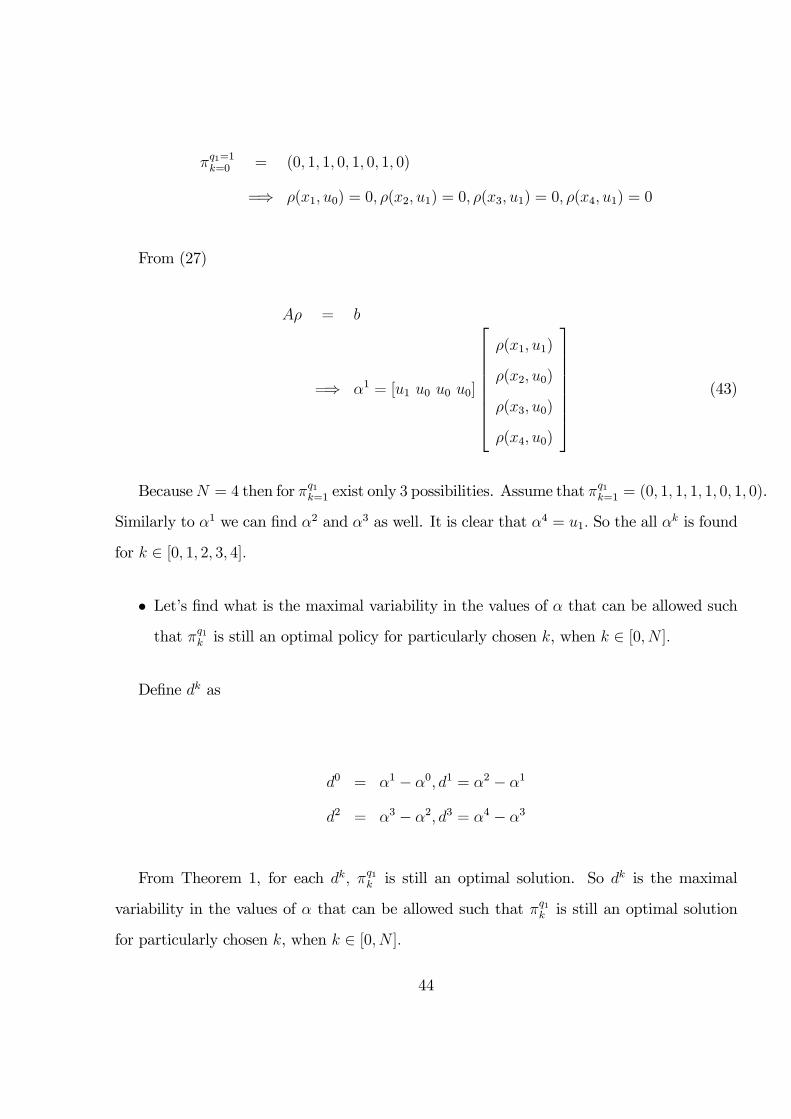
BecauseN = 4 then for πq1k=1 exist only 3 possibilities. Assume that πq1k=1 = (0, 1, 1, 1, 1, 0, 1, 0).

Similarly to α1 we can find α2 and α3 as well. It is clear that α4 = u1. So the all αk is found

for k ∈ [0, 1, 2, 3, 4].

• Let’s find what is the maximal variability in the values of α that can be allowed suchthat πq1k is still an optimal policy for particularly chosen k, when k ∈ [0, N ].

Define dk as

d0 = α1 − α0, d1 = α2 − α1

d2 = α3 − α2, d3 = α4 − α3

From Theorem 1, for each dk, πq1k is still an optimal solution. So dk is the maximal

variability in the values of α that can be allowed such that πq1k is still an optimal solution

for particularly chosen k, when k ∈ [0, N ].

44

• For given α we can find an appropriate αk+1 and αk, where αk+1 > α > αk. After αk+1

and αk are known, we can find πq1k . After πq1k is known the ρ will be found easily from

(27).

• After ρ was found a cost can be calculated from the following formula

cost = [z1 z1 z2 z2 z3 z3 z4 z4]

ρ(x1, u0)

ρ(x1, u1)

ρ(x2, u0)

ρ(x2, u1)

ρ(x3, u0)

ρ(x3, u1)

ρ(x4, u0)

ρ(x4, u1)

(44)

6.1.3 Example of CMDPS Algorithm Application to CMDP Problems

For better understanding of the algorithm let’s consider the following example.

We have four states, where for each state, its cost is equal to the number that is written

in the circles on Figure 6. The transitions probabilities as in Figure 6 with values taken from

(45). The values of control levels and β we can see at (46).

45

0 1 2 3

P0 P7

P1 P3 P5

P2 P4 P6

Figure 6: Markov Chain for Example 1

P0(u0) = 0.8, P0(u1) = 0.9

P1(u0) = 0.2, P1(u1) = 0.1

P2(u0) = 0.6, P2(u1) = 0.7

P3(u0) = 0.4, P3(u1) = 0.3 (45)

P4(u0) = 0.6, P4(u1) = 0.7

P5(u0) = 0.4, P5(u1) = 0.3

P6(u0) = 0.65, P6(u1) = 0.75

P7(u0) = 0.35, P7(u1) = 0.25

u0 = 0.1, u1 = 1, β = 0.99 (46)

From (45) A is easily calculated.

Now let’s answer our questions.

46

• Let’s find αk. We start with α0 and continue according to the algorithm explained

above

α0 = 0.1

π1k=−1 = (1, 0, 1, 0, 1, 0, 1, 0)

I0 = {1, 2, 3, 5, 7}, Ic0 = {4, 6, 8}v = (0, 0, 0, v4, 0, v6, 0, v8)

z = [0 0 1 1 2 2 3 3]

v0 = (0, 0, 0, 0, 0, v4, v6, v8)

z0 = [0 0 1 2 3 1 2 3]

w = [0 0 1 2 3] ∗ (A00)−1

v06,7,8 = [1 2 3]− wAc0

= [−0.4345 − 0.4368 − 0.0023] ¤ 0I0 = {1, 3, 4, 5, 7}, Ic0 = {2, 6, 8}

v06,7,8 = [0 2 3]− wAc0

= [0.4345 − 0.0023 0.4322] ¤ 0

I0 = {1, 3, 5, 6, 7}, Ic0 = {2, 4, 8}

v06,7,8 = [0 1 3]− wAc0

= [0.4368 0.0023 0.4345] ≥ 0= > π1k=0 = (1, 0, 1, 0, 0, 1, 1, 0)

ρ = [0.6302 0 0.2038 0 0 0.1141 0.0519 0]

α1 = 0.2027

47

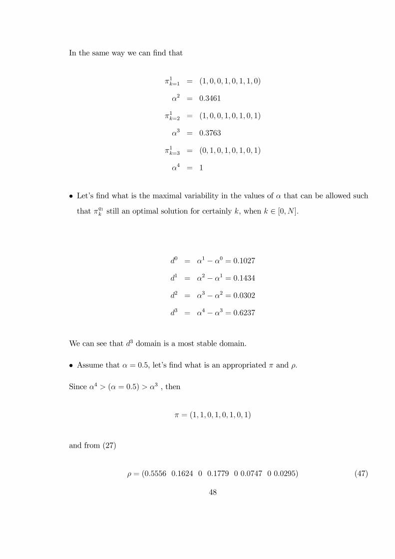
In the same way we can find that

π1k=1 = (1, 0, 0, 1, 0, 1, 1, 0)

α2 = 0.3461

π1k=2 = (1, 0, 0, 1, 0, 1, 0, 1)

α3 = 0.3763

π1k=3 = (0, 1, 0, 1, 0, 1, 0, 1)

α4 = 1

• Let’s find what is the maximal variability in the values of α that can be allowed suchthat πq1k still an optimal solution for certainly k, when k ∈ [0, N ].

d0 = α1 − α0 = 0.1027

d1 = α2 − α1 = 0.1434

d2 = α3 − α2 = 0.0302

d3 = α4 − α3 = 0.6237

We can see that d3 domain is a most stable domain.

• Assume that α = 0.5, let’s find what is an appropriated π and ρ.

Since α4 > (α = 0.5) > α3 , then

π = (1, 1, 0, 1, 0, 1, 0, 1)

and from (27)

ρ = (0.5556 0.1624 0 0.1779 0 0.0747 0 0.0295) (47)

48

• The cost can be calculated from (47) and (44).

cost = 0.4158 (48)

Now we will compare the results which were gotten by CMDPS algorithm to one of the

well known algorithms. The one of the most popular algorithms for LP solving is the Simplex

algorithm, so the comparison will be done to this one.

First of all we are interested to compare the ρ and the cost for α = 0.5. The results that

were gotten by the Simplex algorithm coincide with (47) and (48) as expected.

Now let’s compare the behavior of these two algorithms for the different values of α,

where

α ∈ (u0, u1) = (0.1, 1)

The results of CMDPS algorithm can be written in the following form:

For α = α0, we use in all four states control level u0.

For (α0 = 0.1) < α < (α1 = 0.2027), we have randomization in state 2 and in the rest

states we use control level u0.

For α = α1, in the states 0, 1 and 3 we use control level u0, and in the state 2 we use

control level u1.

For (α1 = 0.2027) < α < (α2 = 0.3461), we have randomization in state 1, in the states

0 and 3 we use control level u0, and in the state 2 we use control level u1.

For α = α2, in the states 0 and 3 we use control level u0, and in the states 1 and 2 we

use control level u1.

For (α2 = 0.3461) < α < (α3 = 0.3763), we have randomization in state 3, in the state 0

we use control level u0, and in the states 1 and 2 we use control level u1.

For α = α3, in the state 0 we use control level u0, and in the states 1, 2 and 3 we use

control level u1.

49

For (α3 = 0.3763) < α < (α4 = 1), we have randomization in state 0 and in the rest

states we use control level u1.

For α = α4, we use in all four states control level u1.

Actually from computational point of view, in order to get these results, we need to find

only 3 values of α : α1, α2, α3. The values of α0 and α4 are known from the beginning

because these values are equal to the minimal and maximal value of control level and so

calculated in the trivial way.

In order to derive the same solution properties by Simplex algorithm (Appendix A) we

need to run a simulation with small enough step for α, so in order to get a precise results

we run the algorithm thousands times. Moreover even after this huge number of runs we

don’t know exactly what happens in the each possible value of α because the number of α’s

is infinite and the number of runs is finite even if it is very big.

On Figure 7 we can see the results that were derived by Simplex method for example 1.

On Figure 8 we can see the randomization behavior for example 1 that were derived by

CMDPS algorithm. The results are the same.

By using a CMDPS algorithm we need to find only 3 values of α.

As was stated in this section, it is enough to find N-1 different points of α, in order to

get the full solution structure.

6.2 CMDPS Algorithm for Finite Number of Control Levels

Now we will extend the analysis from two control levels for the arbitrary, but finite, number

of control levels.

Here we should add one small correction for assumption 2 such that it will suitable for

case with arbitrary number of control levels.

Assumption 2 for arbitrary number of control levels (monotonicity assump-

tion): When the using of higher control levels in state xi is increasing, the value of the

50

0 0.2 0.4 0.6 0.8 10

0.2

0.4

0.6

0.8

1µ(x0,u) versus α

α

µ(x0

,u)

0 0.2 0.4 0.6 0.8 10

0.2

0.4

0.6

0.8

1µ(x1,u) versus α

α

µ(x1

,u)

0 0.2 0.4 0.6 0.8 10

0.2

0.4

0.6

0.8

1µ(x2,u) versus α

α

µ(x2

,u)

0 0.2 0.4 0.6 0.8 10

0.2

0.4

0.6

0.8

1µ(x3,u) versus α

α

µ(x3

,u)

control u0control u1

the first alfa threshold

the second α threshold

the third alfa threshold

Figure 7: The Simplex Method Results

51

Example 1 Results

0

1

2

3

0.1 0.3 0.5 0.7 0.9

Constraint Value

Rand

omiz

atio

n S

tate

Figure 8: Randomization Behavior in Example 1

constraint α is increasing, where xi is the state with randomization. We will say that effec-

tive power control level in state with randomization is higher.

By effective power control level of the state we mean the following:

ueffective(xi) = ρ(xi, u0)u0 + ρ(xi, u1)u1 + ...+ ρ(xi, us)us (49)

where xi is the state and u0, u1.., us are the power control levels.

With a some abuse of notations we will use Theorem 3 and Theorem 4 for the case with

arbitrary, but finite, number of control levels as well. We can do this because from ([1],

Theorem 3.8) we know that for a certain value of α there exists an optimal policy which has

randomization only in one state and this randomization is only between two control levels.

Conclusions: From Theorem 2,3 and 4 we can conclude that if for each α there exists

a unique optimal solution then it takes the following form:

1. For α = u0, π = (u0, u0, ..., u0) is optimal.

52

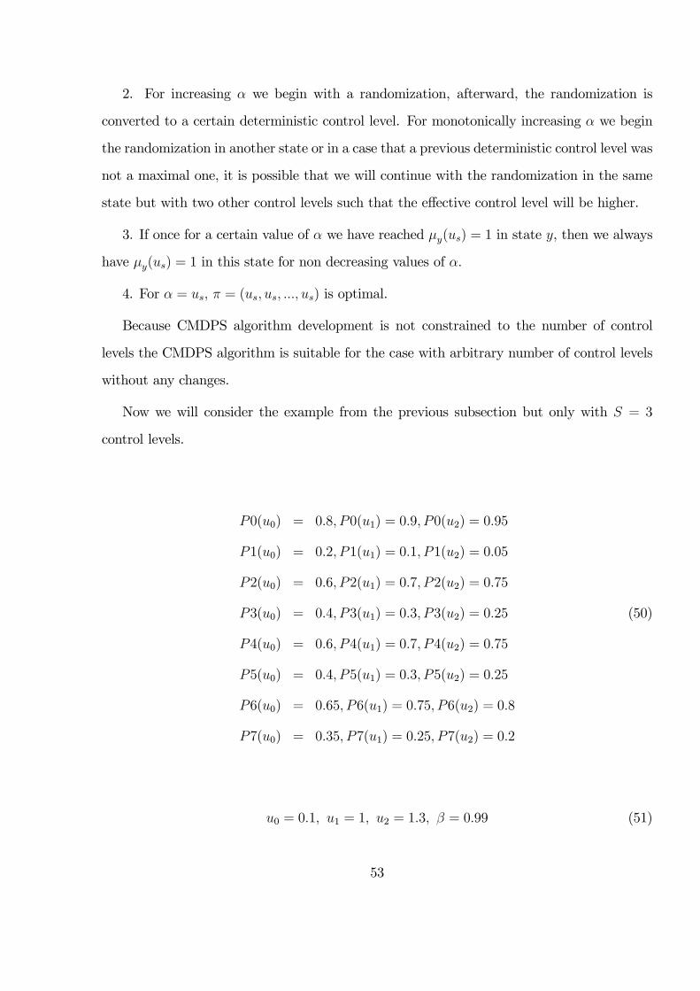
2. For increasing α we begin with a randomization, afterward, the randomization is

converted to a certain deterministic control level. For monotonically increasing α we begin

the randomization in another state or in a case that a previous deterministic control level was

not a maximal one, it is possible that we will continue with the randomization in the same

state but with two other control levels such that the effective control level will be higher.

3. If once for a certain value of α we have reached µy(us) = 1 in state y, then we always

have µy(us) = 1 in this state for non decreasing values of α.

4. For α = us, π = (us, us, ..., us) is optimal.

Because CMDPS algorithm development is not constrained to the number of control

levels the CMDPS algorithm is suitable for the case with arbitrary number of control levels

without any changes.

Now we will consider the example from the previous subsection but only with S = 3

control levels.

P0(u0) = 0.8, P0(u1) = 0.9, P0(u2) = 0.95

P1(u0) = 0.2, P1(u1) = 0.1, P1(u2) = 0.05

P2(u0) = 0.6, P2(u1) = 0.7, P2(u2) = 0.75

P3(u0) = 0.4, P3(u1) = 0.3, P3(u2) = 0.25 (50)

P4(u0) = 0.6, P4(u1) = 0.7, P4(u2) = 0.75

P5(u0) = 0.4, P5(u1) = 0.3, P5(u2) = 0.25

P6(u0) = 0.65, P6(u1) = 0.75, P6(u2) = 0.8

P7(u0) = 0.35, P7(u1) = 0.25, P7(u2) = 0.2

u0 = 0.1, u1 = 1, u2 = 1.3, β = 0.99 (51)

53

From (50) A is easily calculated.

Now let’s answer our questions.

• Let’s find αk. We start with α0 and continue according to the CMDPS algorithm

α0 = 0.1

π1k=−1 = (1, 0, 0, 1, 0, 0, 1, 0, 0, 1, 0, 0)

π1k=0 = (1, 0, 0, 1, 0, 0, 0, 0, 1, 1, 0, 0)

α1 = 0.2307

π1k=1 = (1, 0, 0, 0, 0, 1, 0, 0, 1, 1, 0, 0)

α2 = 0.4020

π1k=2 = (1, 0, 0, 0, 0, 1, 0, 0, 1, 0, 0, 1)

α3 = 0.4265

π1k=3 = (0, 0, 1, 0, 0, 1, 0, 0, 1, 0, 0, 1)

α4 = 1.3

• Let’s find what is the maximal variability in the values of α that can be allowed suchthat πq1k still an optimal solution for certainly k, when k ∈ [0, N ].

d0 = α1 − α0 = 0.2307

d1 = α2 − α1 = 0.1713

d2 = α3 − α2 = 0.0245

d3 = α4 − α3 = 0.8735

We can see that d3 domain is a most stable domain.

54

• Assume that α = 0.5, let’s find what is an appropriated π and ρ.

Since α4 > (α = 0.5) > α3 , then

π = (1, 0, 1, 0, 0, 1, 0, 0, 1, 0, 0, 1)

and from (27)

ρ = (0.6667 0 0.0770 0 0 0.1795 0 0 0.0588 0 0 0.0181) (52)

• The cost can be calculated from (52) and (44).

cost = 0.3514

7 A New Approach to Optimization of Wireless Com-

munications

In this section we will discuss the application of CMDPS algorithm to solving of wireless

communications problems.

Let’s consider a diagram shown in Figure 9 that describes our communications problem.

In this diagram we can see the representation of the following problem:

λ=2[codewords/time duration], R=3[codewords/time duration],

Tslot =1R= 1

3[time duration] and N = 3 (the buffer size is 2).

So in each slot a maximally one codeword can be transmitted. In the left upper corner of

the diagram arcs denote arrivals and straight lines denote transmissions. As we can see in the

first two slots after each arrival we have one transmission and in a third slot only transmission

is presented. This structure can be represented by Markov chain. In this diagram (Figure

9), represented only Markov chain for N = 3, but it is clear that for general N it would be

55

(0,0)

(1,tr1)

(0,1) (1,1)

Ps(u)

1

(1,tr2) (2,tr2)

(0,2) (1,2)

1 1-Ps(u)

1

Ps(u) 1-Ps(u) 1-Ps(u)Ps(u)

Ps(u) 1-Ps(u)

Ps(u)

1

(1,0)

1-Ps(u)

(2,2)

(2,0)

Figure 9: Markov Chain of the Wireless Communications Problem

the only duplicating of this replica. In each state we have two numbers (a, b), where a this

is the number of messages in the buffer and b this is the number of the transmissions that

were completed at the time duration.

Because our control problem is in which power level to use in each transmission, we can

simplify the above diagram by removing states with arrivals only, without transmissions.

There are (1, tr1), (2, tr1), (1, tr2) states. The diagram in Figure 10 represents exactly the

same problem but in a simpler way. We can see that for each main state, main states

56

(0,0)

(0,1) (1,1)

Ps(u)

(0,2) (1,2)

1

1-Ps(u)

Ps(u) 1-Ps(u)

1-Ps(u)1-Ps(u)

Ps(u)

(1,0)

Ps(u) 1-Ps(u)

Ps(u)

1-Ps(u)

(2,2)

(2,0)

Figure 10: Simplified Markov Chain of the Wireless Communications Problem

are the states that represent different number of codewords in the buffer, we have R − 1additional states for each transmission during one time duration. So the maximal number

of necessarily states is RN . The all states will be numerated in the following order: (0, 0) is

a state number 1, (0, 1) is a state number 2, (0, 2) is a state number 3, ..., (1, 0) is a state

number 4, ... (N − 1, 0) is a state number RN −R+ 1 and finally (N − 1, R− 1) is a statenumber RN .

57

7.1 Communications Problem Optimization Using CMDP Ap-

proach

We are interested to minimize the average delay of the transmissions while the average power

remains below a given level α.

We assume a block flat fading Gaussian channel in which the fading of each slot is iid

according to some distribution (such as Rayleigh, Rice etc...). Denote the fading disturbances

at slot k by wk.

Although it is more common to use average cost we are using the discounted cost. It

simplifies the calculation and when the discount factor β → 1 by Tauberian Theorem [10]

we are getting the average cost. Consider a finite CMDP with arbitrary, but finite, number

of control levels and one constraint.

Definitions:

• W is the set of all possible fading disturbances.

• fβ(σ, π;x, u,w) = (1 − β)P∞

t=1 βt−1P π

σ (Xt = x,Ut = u,Wt = w), where w ∈ W and

0 < β < 1.

• Xk is the buffer size at slot k.

• u(xk) ∈ U is a transmitted power at slot k where in the buffer we have xk codewords

waiting for transmission.

• Immediate cost at time k is the number of codewords waiting in the buffer after k stepswhen power u is used in slot k, therefore c = c(xk, u) = xk, where xk is the number of

codewords at slot k.

58

• The discounted cost can be defined using [1] and [4]

C = Cβ(σ, π)

= (1− β)Eπσ{

∞Xk=1

βk−1c(xk, uk)}

= (1− β)∞Xk=1

βk−1Eπσc(xk, uk)

= (1− β)∞Xk=1

Xx,u,w

βk−1P πσ (xk = x,wk = w, uk = u)c(x, u)

=Xx,u

(1− β)∞Xk=1

Xw

βk−1P πσ (xk = x,wk = w, uk = u)c(x, u)

=Xx,u

(1− β)∞Xk=1

βk−1P πσ (xk = x, uk = u)c(x, u) (53)

=Xx,u

fβ(σ, π;x, u)c(x, u)

=Xx,u

fβ(σ, π;x, u)x

• Immediate cost at time k, related to the constraint, is the number of codewords waitingin the buffer after k steps where power u used at slot k, therefore d = d(xk, u) = u,

where xk is the number of codewords at slot k.

• The value of the constraint criterion when starting at σ and using policy π can be

defined as follows

D = Dβ(σ;π)

=Xx∈X

Xu∈U

fβ(σ, π;x, u)d(x, u)

=Xx∈X

Xu∈U

fβ(σ, π;x, u)u

In (53) we used property that c(x, u) doesn’t depend on w, therefore problem can be

solved for average value of disturbances. (the same derivation for d(x, u)).

59

In the next equations we summarize our optimization problem. The optimization problem

is:

minπ

Cβ(σ, π) = minπ

Xx,u

fβ(σ, π;x, u)x

Subject to

Dβ(σ, π) =Xx,u

fβ(σ, π;x, u)u 6 α

We can do one more simplification. The inequality constraint can be replaced by equality

because in practise we are interested to use as much power as we have in order to improve

the delay (higher power will decrease the error probability of the transmission), therefore

Dβ(σ, π) =Xx,u

fβ(σ, π;x, u)u = α

Now by using LP β1 (σ) we can rewrite our problem in a simpler form.

minρ

Xx,u

ρ(x, u)x (54)

Subject to

Xx,u

ρ(x, u)u = α (55)

P

y∈XP

u∈U(y) ρ(y, u)(δx(y)− βPyx(u)) = (1− β)σ(x),∀x ∈ X

ρ(y, u) > 0,∀y, u

Define ρx = ρx(u) =

Px ρ(x, u), and ρu = ρu(x) =

Pu ρ(x, u), so we can rewrite (54)

60

and (55) as following

minρ

Xx,u

ρ(x, u)x

= minρ

Xx

xXu

ρ(x, u)

= minρ

Xx

ρu(x)x

Xx,u

ρ(x, u)u

=Xu

uXx

ρ(x, u)

=Xu

uρx(u) = α

⇒

minρhx, ρu(x)i (56)

Subject to

hu, ρx(u)i = α (57)

P

y∈XP

u∈U(y) ρ(y, u)(δx(y)− βPyx(u)) = (1− β)σ(x),∀x ∈ X

ρ(y, u) > 0,∀y, u

(58)

Define an average delay (ad) in the mean of the number of codewords in the buffer.

Denote the number of codewords in the buffer by "nc", a probability for k codewords in the

buffer by P (nc = k) and express an average delay as follows

61

ad =∞Xk=0

P (nc = k)k (59)

In our design assignment we are interested to answer the following questions:

1. What are the values of αk.

2. What is the maximal variability in average power α that can be allowed such that πq1k

still an optimal solution for certain value of k, when k ∈ [0, N ].

3. For given α what is an optimal solution π and what is the value of appropriate ρ.

4. What is an average delay.

The CMDPS algorithm will help us to answer these questions.

7.2 CMDPS Algorithm Application in Wireless Communications

In our model we assume a BPSK modulation without any coding and our Markov diagram

as in Figure 11. We can see that the transitions at final states a little bit differ from the other

because when the buffer is full and arriving is happening we lost an arrival word immediately.

The transition probabilities are calculated according to (65) in Appendix C.

Simulation Conditions:

λ = 2 [words/ sec], R = 3 [words/ sec]

Tslot =1

R=1

3[sec]

β = 0.99, N = 3

Eb0 = 0.1 [Joules], Eb1 = 1 [Joules] (Appendix C)

x1 = 0 [words], x2 = 1 [words], x3 = 2 [words], x4 = 3 [words]

N0

2= 1, ζ2 = 1 (Appendix C)

Tb = 0.1 [sec] (Appendix C)

u0 =Eb0Tb

= 1 [W ], u1 =Eb1Tb

= 10 [W ]

62

(0,0)

(0,1) (1,1)

Ps(u)

(0,2) (1,2)

1

1-Ps(u)

Ps(u) 1-Ps(u)

1-Ps(u)

1-Ps(u)

Ps(u)

1-Ps(u)

Ps(u)

(1,0)

(2,1)

1-Ps(u)Ps(u)

1-Ps(u)

Ps(u)1-Ps(u)

(2,2)

(2,0)

Ps(u)

Ps(u)

Figure 11: Markov Chain for Communications Problem Example

63

For simplicity we will run simulation for two control levels but as we saw in section 6.2

it could be done for the arbitrary, but finite, number of control levels.

state number label on the diagram randomization order

1 (0,0) 1

2 (0,1) 5

3 (0,2) 9

4 (1,0) 7

5 (1,1) 4

6 (1,2) 2

7 (2,0) 6

8 (2,1) 3

9 (2,2) 8

Questions 1 and 2:

state number αk dk

1 α1 = 0.3141 d0 = 0.3141

6 α2 = 0.4844 d1 = 0.1703

8 α3 = 0.5053 d2 = 0.0210

5 α4 = 0.5806 d3 = 0.0753

2 α5 = 0.7685 d4 = 0.1878

7 α6 = 0.7716 d5 = 0.0031

4 α7 = 0.7900 d6 = 0.0184

9 α8 = 0.7990 d7 = 0.0090

3 α9 = 1 d8 = 0.2010

Questions 3 and 4:

Assume that α3 > α = 0.5 > α2, then

π = (0, 1, 1, 0, 1, 0, 1, 0, 1, 0, 0, 1, 1, 0, 1, 1, 1, 0)

64

ρ = (0, 0.2871, 0.2426, 0, 0.1563, 0, 0.0396, 0, 0.0736, 0,

0, 0.1448, 0.0100, 0, 0.0046, 0.0125, 0.0288, 0)

ad =∞Xk=0

P (nc = k)k

=4X

k=1

Xu

ρ(xk, u)xk

= 0.3699 [words]

65

8 Conclusions and Further Research

In this research we derived a new solution methods for constrained Markov decision processes

and considered applications of these methods to the optimization of wireless communications.

In this paper we concentrated on the problem of infinite amount of information transfer over

a fading channel. We seceded to minimize the transmission delay under the average power

constraint where at each slot we use one of the available discrete power levels, while maximal

power level is limited by a peak power constraint. Moreover we developed an innovative

algorithm which ,aside of optimization problem solving, is able to show sensitivity of the

solution to changes in the average power level. The results show that by using a new

developed algorithm we can get a general and simple solution of the problem.

For further research we would like to propose the following:

• Extension of the fundamental Theorems to the case with arbitrary number of con-straints.

• Extension of the constraints to inequality cases.

• Extension to finite horizon problems.

66

Appendix A: Linear Programming (LP) and Simplex

Method Idea

In this Appendix we will discuss about LP and usage of Simplex Method for its solution.

Consider the following linear programming problem.

Minimize c1x1 + c2x2 + ...+ cnxn

Subject to a11x1 + a12x1 + ...+ a1nxn ≥ b1

a21x1 + a22x1 + ...+ a2nxn ≥ b2

.

.

.

am1x1 + am2x1 + ...+ amnxn ≥ bm

x1, x2, .., . , xn ≥ 0

Here c1x1 + c2x2 + ... + cnxn is the objective function to be minimized. The coefficients

c1, c2, ..., cn are the cost coefficients and x1, x2, ..., xn are the decision variables to be deter-

mined. The inequalityPn

j=1 aijxj ≥ bi denotes the ith constraint. The coefficients aij for

i = 1, 2, ...,m, j = 1, 2, ..., n are called the technological coefficients. These technological

coefficients form the constraint matrix A.

67

A =

a11 a12 . . . a1n

a21 a22 . . . a2n

. . .

. . .

. . .

am1 am2 . . . amn

The column vector whose ith component is bi, which is referred to as the right-hand side

vector, represents the minimal requirements to be satisfied. The constraints x1, x2, ..., xn ≥ 0are the nonnegativity constraints. A set of variables x1, x2, ..., xn satisfying all the constraints

is called a feasible point or a feasible vector. The set of all such points constitutes the feasible

region or the feasible space.

The linear programming problem can be stated as follows: Among all feasible vectors,

find one that minimizes (or maximizes) the objective function.

The idea of the finding of the LP problem solution can be represented Geometrically in

the Figure 12. Let consider the following problem

Minimize c · xs.t. A · x ≥ b

x ≥ 0

A feasible region consists of all vectors x satisfying Ax ≥ b and x ≥ 0. Among all suchpoints we wish to find a point with minimal cx value. In order to minimize the cost we

need to move in the direction that do this minimization. This direction is −c, and hence theplane is moved in this direction as much as possible. This process is illustrated in Figure 12,

where x∗ is an optimal point. Needless to say, for a maximization problem, we need to move

as much as possible in the direction c.

68

Figure 12: Geometric Solution

Now we will give a brief explanation of the Simplex method idea.

Consider the system A ·x = b and x ≥ 0, where A is an m×n matrix and b is a vector of

length m. Suppose that rank(A, b) = rank(A) = m. After possibly rearranging the columns

of A, let A = [B,N ] where B is an m×m invertible matrix and N is an m× (n−m) matrix.

The solution x =

XB

XN

to the equations Ax = b, where

XB = B−1 · b

and

XN = 0

is called a basic solution of the system. If XB ≥ 0, then x is called a basic feasible solution

of the system. Here B is called the basic matrix (or simply the basis) and N is called the

nonbasic matrix. The components of XB are called basic variables and the the components

of XN are called nonbasic variables.

The key to the simplex method lies in recognizing the optimality of a given basic feasible

69

Figure 13: Simplex Method - Geometric Motivation

70

solution (extreme point solution) based on local considerations without having to (globally)

enumerate all basic feasible solutions.

Let discuss a Geometric motivation of Simplex method. Consider the following LP prob-

lem

minx

c · xA · x = b

x ≥ 0

Figure 13 illustrates the situation in 2 dimensions, where n = 6, m = 4 and where

XB = {x3, x4, x5, x6}. The defining variables associated with n = 6 hyperplanes on this

figure. The vertices or extreme points of the feasible region are labeled as v1, ..., v5 and c is

the cost vector. The current basic feasible solution corresponds to the vertex v1,that is, the

origin. Now consider the origin v1 and examine the two defining hyperplanes associated with

the corresponding nonbasic variables. Holding one of these hyperplanes binding and moving

in a direction, feasible to the remaining hyperplane, takes us along a one-dimensional ray

with vertex at v1. There are two such rays. Holding x2 = 0 and increasing x1 takes us along

the x1 axis. Similarly, holding x1 = 0 and increasing x2 takes us along the x2 axis. Assume

that latter direction is better (from point of minimization view) then we move along the x2

axis. Naturally we would like to move as far as possible along this edge since as far we are

going as more we minimize the objective function (the angle between x2 and −c is acute).However, our motion is blocked by the hyperplane x3 = 0, since x3 has been driven to zero

and moving any further would drive x3 negative. If no such blocking hyperplane existed,

then the optimal solution value would have been unbounded. Furthermore, since one linearly

independent hyperplane was binding all along and we were blocked by a new hyperplane, we

now have two linearly independent hyperplanes binding, and so we are at another extreme

point of the feasible region. At v2 the nonbasic variables are x1 and x3, and the remaining

variables are basic. We have now completed one step known as the iteration or pivot of the

71

simplex method. In this step the variable x2 is called the entering variable since it entered

the set of basic variables, and the variable x3 is called the blocking variable, or the leaving

variable, since it blocked our motion or left the set of basic variables at v1.

Repeating this process at v2, we would of course not like to enter x3 into the basis

since it will only take us back along the reverse of the previous direction. However, holding

x3 = 0 and increasing x1takes us along an improving edge because this direction is making

an acute angle with −c direction (Figure 13). Proceeding in this direction we notice thatmore than one hyperplane blocks our motion. Suppose we arbitrarily choose one of them,

namely x4 = 0 as the blocking hyperplane. Hence x4 is the leaving variable, and for current

basis representation of v3, x3 and x4 are the nonbasic variables. Now if we hold x4 = 0 and

move in a direction along which x3 increases, the objective function value decreases since this

direction is making acute angle with −c direction. However, this direction is not feasible.We are blocked by the hyperplane x5 = 0 even before we begin to move. That is, x5 leaves

the basis giving x4 and x5 as our new non basis variables, while we are still at the same

vertex v3. With x4 and x5 as the nonbasic variables at v3, holding x5 = 0 and increasing x4

takes us along an improving, feasible edge direction. The blocking variable that gets driven

to zero is x6, and the new nonbasic variables are x5 and x6. Observe that corresponding to

this basis, none of the two rays, defined by holding one of the nonbasic variables equal to

zero and increasing the remaining nonbasic variable, lead to an improvement in the objective

function, and so our "key result" declares v4 to optimal solution.

72

Appendix B: Principle of Optimality and Value Iteration

Algorithm

The dynamic programming (DP) technique rests on a very simple idea, the principle of

optimality. Roughly, the principle of optimality states the following rather obvious fact.

Principle of Optimality: [4]

Let π∗ = {π0, π1, ..., πN−1} be an optimal policy for the basic problem, and assume thatwhen using π∗, a given state xi occurs at time i with positive probability. Consider the

subproblem whereby we are at xi and wish to minimize the "cost-to-go" from time i to time

N .

E

(gN(xN) +

N−1Xk=i

gk(xk, πk(xk), wk)

). Then the truncated policy {πi, πi+1, ..., πN−1} is optimal for this subproblem.

The intuitive justification of the principle of optimality is very simple. If the truncated

policy {πi, πi+1, ..., πN−1} were not optimal as stated, we would be able to reduce the costfurther by switching to an otptimal policy for the subproblem once we reach xi. The prin-

ciple of optimality suggests that an optimal policy can be constructed in piecemeal fashion,

first constructing an optimal policy for the "tail subproblem" involving the last stage, then

extending the optimal policy to the "tail subproblem" involving the last two stages, and

continuing in this manner until an optimal policy for the entire problem is constructed.

Value iteration is the most widely used and best understood algorithm for solving dis-

counted Markov decision problems. The following value iteration algorithm finds a stationary

ε-optimal policy, (dε)∞, and an approximation to its value.

Value Iteration Algorithm: [8]

1. Select v0 ∈ V, specify ε > 0, and set n = 0.

73

2. For each x ∈ X, compute vn+1(x) by

vn+1(x) = maxu∈U(x)

{r(x, u) +Xj∈X

βP (j|x, u)vn(j)} (60)

where r(x, u) is a reward at state x ∈ X using action u ∈ U, and P (j|x, u) is a transitionprobability to state j from state x using action u.

3. If °°vn+1 − vn°° < ε

1− β

2β(61)

go to step 4. Otherwise increment n by 1 and return to step 2.

4. For each x ∈ X, choose

dε(x) ∈ arg maxu∈U(x)

{r(x, u) +Xj∈X

βP (i|x, u)vn(j)} (62)

and stop.

The following theorem provides the main results regarding convergence of the above value

iteration algorithm.

Theorem ([8], Theorem 6.3.1)

Let v0 ∈ V, ε > 0, and let {vn} satisfy (60) for n ≥ 1. Then

• vn converges in norm to v∗β,

• finite N for which (61) holds for all n ≥ N,

• the stationary policy (dε)∞ defined in (62) is ε-optimal, and

• °°vn+1 − v∗β°° < ε/2 whenever (61) holds.

74

Appendix C: BPSK Modulation in Fading Environment

In this section we will give a brief description of the BPSK modulation [6] and an impact of

the channel fading for the error probability calculation [7].

Definitions:

• Eb is the transmitted signal energy per bit.

• Tb is the time duration of one bit transmission.

• fc is the carrier frequency.

BPSK (Binary phase-shift keying) is a modulation where, the pair of signals, s1(t) and

s2(t), used to represent binary symbols 1 and 0, respectively, are defined by

s1(t) =

r2Eb

Tbcos(2πfct) (63)

s2(t) =

r2Eb

Tbcos(2πfct+ π)

= −r2Eb

Tbcos(2πfct) (64)

A pair of sinusoidal waves, s1(t) and s2(t), differing only in phase by 180 degrees, as

defined above, are named antipodal signals. Using Gram-Schmidt orthogonalization we find

a single basis function, namely

φ1(t) =

r2

Tbcos(2πfct), 0 ≤ t ≤ Tb

Thus, we may express the transmitted signals s1(t) and s2(t) in terms of φ1(t) as follows

s1(t) =pEbφ1(t)

s2(t) = −pEbφ1(t)

75

Here we will skip the part of probability of error derivation because it quite technical and

can be seen in [6]. We will give only the final formula:

Pr{ε} = Q

Ãr2Eb

N0

!

where

Q (x) =1√2π

Z ∞

x

exp(−z2

2)dz

For a fading channel we have one additional modification, this is factor r2. For block

fading Gaussian channel in which the fading of each slot is iid according to Rayleigh distrib-

ution, the error probability for one bit transmission can be expressed by a following formulas

[6] and [7]:

Pr{ε} = Q

Ãs2r2Eb

N0

!

where Rayleigh distribution of random variable r is expressed as follows

f(r) =r

σ2e−

r2

2σ2 , r ≥ 0

Because we used letter σ for another purpose (initial distribution) before, we will replace

σ2 here by letter ζ2, and from now on

f(r) =r

ζ2e− r2

2ζ2 , r ≥ 0

Pr{ε}avr =

Z ∞

0

Q

Ãs2r2Eb

N0

!f(r)dr =

1

2

"1−

sEb/N0

1 +Eb/N0

#where Eb = E{r2Eb} = 2ζ2Eb

⇒ A probability of one bit successful transmission is expressed as follows

76

Psucc = Ps = 1− 12

"1−

sEb/N0

1 +Eb/N0

#(65)

References

[1] E. Altman, Constrained Markov Decision Processes, Chapman&Hall/CRC,1998

[2] E. Altman, Applications of Markov Decision Processes in Communication Networks,

INRIA B.P. 1993

[3] M.S. Bazaraa, J.J. Jarvis, H.D. Sherali, "Linear Programming and Network Flows",

John Wiley&Sons, 1990

[4] D.P. Bertsekas, Dynamic Programming and Optimal Control, Athena Scientific, Bel-

mont, Massachusetts, 1995

[5] I. Bettesh, Information and Network Theory Aspects of Communication Systems in

Fading Environment, PhD Thesis, October 2002

[6] Simon Haykin, Communication Systems, Second Edition, John Wiley&Sons, 1983

[7] I. Kalet, Lecture notes - Cellular Communications, Winter 2003

[8] Martin L. Puterman, Markov Decision Processes, John Wiley&Sons, 1994

[9] S.M. Ross, Introduction to Stochastic Dynamic Programming,Academic Press, 1983

[10] A. Shwartz, Lecture notes - Control of Stochastic Processes, October 2003

[11] J. Walrand, An Introduction to Queueing Networks, Prentice Hall, 1988

[12] H. Wang and N.B. Mandayam, Opportunistic File Transfer over a Fading Channel

under Energy and Delay Constraints, Asilomar Conference on Signals, Systems and

Computers, Monterey, California, November 2001

77

קובים מאולצים תהליכי החלטה מר בתקשורת אלחוטיתויישומם

ני'אלכסנדר זדורוז

תהליכי החלטה מרקובים מאולצים בתקשורת אלחוטיתויישומם

חיבור על עבודת גמר

קבלת התוארלשם מילוי חלקי של הדרישות ל

מגיסטר למדעים בהנדסת חשמל

ני' אלכסנדר זדורוז

מכון טכנולוגי לישראל–הוגש לסנט הטכניון

2004 חיפה יוני ד'' תשסןסיוו

ורץאדם ש' בהנחיית פרופה ת נעשעבודת הגמר

.בפקולטה להנדסת חשמל

שורץאדם' תודתי והוקרתי לפרופ

על הדרכתו ועזרתו

.בכל שלבי המחקר

אני מודה לטכניון על תמיכה הכספית הנדיבה

.השתלמותיב

תוכן העניינים עמוד

1...................................................................................תקציר

2...........................................................רשימת סמלים וקיצורים

..4...............................................................................מבוא .1

5..................................................סקר ספרות ומטרות המחקר .2

7...................................................אלחוטיתמודל של תקשורת .3

וגישה של תכנות ) CMDP(ובים מאולצים תהליכי החלטה מרק .4

10............................................................................ליניארי

4.1 CMDP.............................................................................................10

CMDP.......................................12 עבור בעיות של תאופטימאלי מדיניות 4.2

LP(.................................................13( תברות ותכנות ליניאריסה מידת ה4.3

CMDP.......................................18 עבור תאופטימאלימדיניות .5

KKT.(..............................................................18(תקר -קון- תנאי קרוש5.1

22...............................................................................יים משפטים יסוד5.2

עבור בעיות של חיסכון תאופטימאליתכונות של מדיניות .6

29............................................................................בהספק

.35.........................................בקרה עבור שתי רמות CMDPSאלגוריתם 6.1

CNDPS......................................................................................37אלגוריתם 6.1.1

CMDPS.........................................................................39 שימוש באלגוריתם 6.1.2

CMDP....................................45 בבעיותCMDPSדוגמא לשימוש באלגוריתם 6.1.3

50.............................. עבור מספר סופי של רמות הבקרהCMDPS אלגוריתם 6.2

)המשך (תוכן העניינים

עמוד

55.................אופטימיזציה בתקשורת אלחוטיתגישה חדשה עבור .7

..CMDP................58 י שימוש בגישת" בעיית תקשורת ע אופטימיזציה של7.1

62................................ בתקשורת אלחוטית CMDPS שימוש באלגוריתם 7.2

66.........................................................עתידימסקנות ומחקר .8

67...................י ורעיון של שיטת הסימפלקס תכנות ליניאר– Aנספח

Value Iteration.......73 ואלגוריתם ת עיקרון האופטימאליו– Bנספח

75........................................ בערוצי דעיכהBPSK אפנון – Cנספח

77................................................................................מקורות

I.............................................................)......... עברית (תקציר

רשימת ציורים

עמוד מספר

8.....................................................................................מודל של תקשורת אלחוטית .1

30..............................................................כחה של מונוטוניותוב עבור הושרשרת מרק .2

30......................................................................................................זוג של מערכות .3

36................................................................................................שינוי הרנדומיזציה .4

CMDPS.........................................................................40 של אלגוריתם הדיאגראמ .5

46.......................................................................וב עבור דוגמא ראשונה שרשרת מרק .6

51................................................................................תוצאות של שיטת הסימפלקס .7

52................................................................התנהגות הרנדומיזציה בדוגמא הראשונה .8

56.....................................................וב עבור בעיה של תקשורת אלחוטיתשרשרת מרק .9

57........................................וב מפושטת עבור בעיה של תקשורת אלחוטיתשרשרת מרק .10

63........................................................ תקשורתיתיוב עבור דוגמא של בעשרשרת מרק .11

69....................................................................................................גיאומטריפתרון .12

70..............................................................גיאומטרית מוטיבציה –שיטת הסימפלקס .13

I

תקציר

ומחשבים םסלולארייההשימוש בטלפונים והתפתחות בשירותי תקשורת אישיים ה

תקשורת ספק הסוללה באמצעיון בצריכת ה לכן חיסכ. משנה לשנהיםגובר ניידים

יתחוטיים בתמיכה בתקשורת אל אחד הגורמים המרכז. חשיבות רבההוא בעלאלה

מצד שני ו ,זה הוא מאד חשובסכון מצד אחד חי .חיסכון מרבי בצריכת ההספקהוא

הספק –ית אמינה של תקשורת אלחוטפקודהיכול לגרום לבעיה רצינית בתהוא

לכן בזמן שמנסים . התקשורת נמוך יכול לגרום לשגיאות שידור ופגיעה באיכות

.לחסוך הספק חייבים לדאוג לאיכות השירות של המשתמש

בדרך כלל פתרונות אלה . ה זובשנים האחרונות הוצעו מספר שיטות הפתרון לבעי

הממוצעת תוך אילוץ על יהההשה מזעור עבור תאופטימאלימדיניות מוצאים

אחרות עבור ,כמה מהן פותחו עבור פתרון של הבעיות בזמן רציף .הספק הממוצעה

שיטות שמטפלות בבעיות בזמן רציף הן כלליות יותר אבל לא תמיד אפשר . זמן בדיד

סוג התקשורת הנפוץ ביותר בשנים ואהפרתית שס ליישם אותן בתקשורת

לא מספיק כלליות בהרבה , עבור זמן בדיד ,שיטות שפותחו עד עכשיו. האחרונות

בדרך כלל בתקשורת .רק עבור שתי רמות בקרההן מוגבלות למשל .מקרים

השהיה ספרתית אנחנו מתעניינים במציאת מדיניות האופטימאלית שממזערת

הבקרה מקסימאלי ומשתמשת רק ברמותממוצע ול הספק הממוצעת תחת אילוץ ע

.אף אחד מהשיטות הקיימות לא יכולה לספק את זה. הנתונות

ים ובה מרקהחלטמפתחים שיטות פתרון חדשות עבור תהליכי במחקר הזה אנחנו

אנחנו . תקשורת אלחוטיתבבעיות אופטימיזציה של מןמאולצים ודנים בישו

במחקר אנחנו מציעים . עם ניתוח ביצועיהן הקיימות שיטות הבקרה קרים את וס

ההשהיה אלחוטית שממזערת את שיטה חדשה של בקרת הספק בתקשורת

כאשר אנחנו מוגבלים לשימוש ,מקסימאליממוצע והממוצעת תחת אילוץ על הספק

שפותחה במהלך טכניקה השיטה הזאת מבוססת על. רק ברמות הבקרה הנתונות

. עם אילוציםוביםמרקהחלטה המחקר עבור תהליכי

II

יותר מכך אנחנו פיתחנו אלגוריתם שמסוגל חוץ מפתרון של בעיית האופטימיזציה

ברמת ההספק הממוצע םלנתח את הרגישות של הפתרון האופטימאלי לשינוי גם

.באילוץ

העברה קצב , יההשה( חד של מחיר זאת אנחנו מתארים מצב כאשר סוג אבעבודה

נשאר ...) יההשה, הספק( מחיר אחר של יות ממוזער תוך כדי שסוגצריך לה) וכדומה

. בעיית אופטימיזציה מאולצתזוהילכן . רמה נתונהל מתחת

של סוגי מידע יסימולטאנצורה כזאת המאפשרת שידור רשתות תקשורת בנויות ב

יית הים הוא הש מדד לביצועבדרך כלל... ואוידי, העברת קבצים, קול :שונים

סוגים שונים של מידע ... שגיאה בשידורהות הסתבר, הספקה צריכת, השידור

י דרישות שונות עבור "גם עסטטיסטית שלהם ו תכונות שני לפיהמובדלים אחד מ

יה שההשההודעות דרוש אינטראקטיבי של עבור שידור, לדוגמא. יםהביצוע

בשידורי אדמחשובה יה ההגבלה על ההשה .הממוצעת מקצה לקצה תהיה מוגבלת

במידע וההשהיה עוברת את הגבול . שניות0.1 יה מוגבלת ל ההשה-מידע קולי

עבור העברת קבצים לא .איכות הקול יורדת בצורה דרמטית, המותר

קצב ולמקסם את יהחנו בדרך כלל רוצים למזער את ההשהאינטראקטיבית אנ

.ההעברה

של) או מקסום(ן מזעור תמיד קיימת ניגודיות בימאולצות טימיזציה אופבבעיות

תוך כדי שסוג אחר של המחיר, יה או קצב העברהלמשל השה, סוג אחד של מחיר

יההכדי למזער את ההש. נמצא מתחת לרמה הנדרשת) יהצריכת הספק או השה(

ותמפני שזה יגדיל את הסתבר, אנחנו צריכים לשדר בהספק הכי גבוה שאפשר

.ידורים החוזרים שיקטין את מספר הש,ההצלחה של השידור

נצרך אנחנו מעוניינים לשדר בהספק העל מנת להקטין את ההספק , בניגוד לזה

הבעיה שלנו ניתנת לניסוח כבעיית של תהליכי ההחלטה . המינימאלי האפשרי

יהואפים למזער את המחיר המיוחס להשהש בה אנחנו , עם אילוציםוביםמרק

.יוהמקסימאלכתלות באילוץ על ההספק הממוצע

III

.אנחנו יכולים לחלק את העבודות בתחום של חיסכון באנרגיה לשני סוגים

.מידע לשידורה בהנחה שיש לנו הספקה סופית של בקרת הצריכה באנרגי– ראשון

.מידע לשידורהנחה שיש לנו הספקה אינסופית של בקרת הצריכה באנרגיה ב–שני

מידע הספקה אינסופית של –של הבעיות במחקר הזה אנחנו מתרכזים בסוג שני

בעבודה הזו אנחנו מנסים להרחיב את השיטות הקיימות למקרים יותר . לשידור

. של רמות הבקרה, אבל סופי, הרחבה משתי רמות הבקרה למספר כלשהו–כלליים

של הפתרון ממבט שלא היה ידוע עד י אנחנו מנתחים את המבנה האופטימאלבנוסף

בהקשר של . לשינויים באילוץתשל המדיניות האופטימאלי" תרגישו "- עכשיו

הזה אנחנו את הנושא . חדש שהוגדר תוך כדי המחקרג ש מוזהבעיית התקשורת

ובגישה , וגם מבחינה נומרית גם מבחינה אנליטית –לית הצלחנו לנתח בצורה די כל

,ילוץהתוצאות שהתקבלו הן שעבור שינויים מספיק קטנים ברמת הא. חדשה

הצלחנו גם . לא משתנה, תבמצבים שהיא דטרמיניסטי, האופטימאליתדיניות המ

.למצוא את התחומים המדויקים עבור השינויים האלה

תארים את המבנה של מבמהלך המחקר אנחנו גם הצלחנו לפתח שני משפטים ש

שני . ייםלמאולצים כל וביםמרק עבור תהליכי החלטה יהאופטימאלהפתרון

במהלך המחקר גם פותח . ם פותחו עבור הנושא של חיסכון בהספק נוספימשפטים

בעיות של תהליכי החלטה מקורי שבאמצעותו אנחנו יכולים לפתור אלגוריתם

התוצאות . ברמת האילוץמאולצים וגם לנתח רגישות הפתרון לשינויים ובים מרק

ל י הפעלה ש"י הרצת האלגוריתם הזה הושווה לתוצאות שהתקבלו ע"שהתקבלו ע

. ברור לאלגוריתם החדש שפיתחנויתרוןעם שיטת הסימפלקס

הפתרון החדשה שפיתחנו עבור בעיות תשיטבסופו של דבר הצלחנו ליישם את

, כלליות, היתרונות העיקריים של שיטה החדשה הם פשטות. אלחוטיתבתקשורת

.חידוש יחסית לשיטות הקודמותו