constraint of the co rise by new atmospheric carbon ...€¦ · click here for full article...

ClickHere

for

FullArticle

Constraint of the CO2 rise by new atmospheric carbon isotopicmeasurements during the last deglaciation

Anna Lourantou,1 Jošt V. Lavrič,1,2 Peter Köhler,3 Jean‐Marc Barnola,1,4 Didier Paillard,2

Elisabeth Michel,2 Dominique Raynaud,1 and Jérôme Chappellaz1

Received 17 April 2009; revised 10 December 2009; accepted 29 January 2010; published 17 June 2010.

[1] The causes of the ∼80 ppmv increase of atmospheric carbon dioxide (CO2) during thelast glacial‐interglacial climatic transition remain debated. We analyzed the parallelevolution of CO2 and its stable carbon isotopic ratio (d13CO2) in the European Project forIce Coring in Antarctica (EPICA) Dome C ice core to bring additional constraints.Agreeing well but largely improving the Taylor Dome ice core record of lower resolution,our d13CO2 record is characterized by a W shape, with two negative d13CO2 excursionsof 0.5‰ during Heinrich 1 and Younger Dryas events, bracketing a positive d13CO2

peak during the Bølling/Allerød warm period. The comparison with marine records andthe outputs of two C cycle box models suggest that changes in Southern Oceanventilation drove most of the CO2 increase, with additional contributions from marineproductivity changes on the initial CO2 rise and d13CO2 decline and from rapidvegetation buildup during the CO2 plateau of the Bølling/Allerød.

Citation: Lourantou, A., J. V. Lavrič, P. Köhler, J.‐M. Barnola, D. Paillard, E. Michel, D. Raynaud, and J. Chappellaz (2010),Constraint of the CO2 rise by new atmospheric carbon isotopic measurements during the last deglaciation, Global Biogeochem.Cycles, 24, GB2015, doi:10.1029/2009GB003545.

1. Introduction

[2] Atmospheric CO2 is the most important anthropogenicgreenhouse gas and arguably the largest contributor to thecurrent global warming [Intergovernmental Panel on ClimateChange, 2007]. The monitoring of its stable carbon isotopicratio (d13CO2) evolution is useful for the identification ofbiogeochemical processes driving the observed variations inCO2. Former studies [Friedli et al., 1986; Francey et al.,1999] provided decisive evidence for the manmade originof the CO2 rise during the last 200 years, based on a ∼1.5‰decline of d13CO2 to its modern value of −7.8‰. Thisdecrease is caused by the 13C‐depleted signature of the twomajor anthropogenic CO2 sources, fossil fuel burning andcarbon release from deforestation, having d13CO2 values of∼−30‰ and −25‰, respectively.[3] In contrast, natural changes in CO2, such as the

80 ppmv rise over Termination I (hereafter TI), i.e., thetransition from the Last Glacial Maximum (LGM) ∼20 kyr B.P.to the Early Holocene (EH, ∼10 kyr B.P.), are still not wellunderstood. Modeling studies attribute it to various oceanic

processes, but without consensus on their relative importance[Broecker and Peng, 1986; Watson and Naveira Garabato,2006]. Two major mechanisms in the ocean are usuallyinvoked to explain the CO2 glacial‐interglacial (G‐IG)changes: (1) a physical one, mainly related to SouthernOcean ventilation changes eventually releasing during Ter-minations old carbon stored in the deep ocean during thepreceding glaciation [Toggweiler, 1999] and (2) a biologicalone, involving the efficiency of nutrient utilization by phy-toplankton in the austral ocean, with decreased efficiency(and thus lower CO2 uptake) when atmospheric dust fertil-ization gets reduced [Archer et al., 2000; Sigman and Boyle,2000]. For more than 3 decades, scientists tried to disen-tangle the relative role of these or alternative processes, suchas changes in oceanic pH and carbonate compensation[Archer et al., 2000], in the evolution of atmospheric CO2.Currently, few models can reproduce the observed amplitudein G‐IG CO2 rise; they succeed only if all processes relevanton these timescales are considered [Köhler et al., 2005a;Brovkin et al., 2007].[4] To validate their hypothesis or to propose alternative

ones, more observational constraints are needed. Paleoatmo-spheric d13CO2 makes one of them and is central to our study.So far, a unique record of atmospheric d13CO2 through TI(including ∼15 measurements) has been obtained from theTaylor Dome (TD) ice core [Smith et al., 1999; SM1999hereafter], filling the time jigsaw between LGM and EH firstproduced from the Byrd core [Leuenberger et al., 1992].Although of coarse resolution, the TD d13CO2 record hasalready been used to evaluate the output of several carbon (C)

1Laboratoire de Glaciologie et Geophysique de l’Environnement,Université Joseph Fourier–Grenoble, CNRS, St Martin d’Hères, France.

2Laboratoire des Sciences du Climat et de l’Environnement, IPSL,Université Versailles‐St Quentin, CNRS, Gif‐sur‐Yvette, France.

3Alfred Wegener Institute for Polar and Marine Research,Bremerhaven, Germany.

4Deceased 2009.

Copyright 2010 by the American Geophysical Union.0886‐6236/10/2009GB003545

GLOBAL BIOGEOCHEMICAL CYCLES, VOL. 24, GB2015, doi:10.1029/2009GB003545, 2010

GB2015 1 of 15

http://dx.doi.org/10.1029/2009GB003545

cycle models [Schulz et al., 2001;Brovkin et al., 2002;Köhleret al., 2005a;Obata, 2007]. For instance [Obata, 2007], usinga coupled climate‐C cycle model, simulates a decrease in netprimary productivity and soil respiration during the YoungerDryas, in agreement with a combined increase of atmosphericCO2 and minimum of d13CO2 observed in the TD ice core atthat time. [Brovkin et al., 2002] emphasize the role of theG‐IG reduced biological pump to explain the simultaneousCO2 increase and d13CO2 decrease suggested by the TDdata during the early part of the Termination.[5] In this study we (1) present a new highly resolved

record of CO2 and d13CO2 across TI from the EuropeanProject for Ice Coring in Antarctica (EPICA) Dome C(EDC) ice core, (2) compare it to existing ice core data (CO2

from EDC [Monnin et al., 2001] and d13CO2 from TD(SM1999)), (3) propose a qualitative scenario on the causesof the deglacial CO2 rise, based on a comparison with otherproxies, and (4) test this scenario with two C cycle boxmodels [Köhler et al., 2005a; Paillard et al., 1993].

2. Method

[6] A detailed description of the experimental method isprovided by Lourantou [2009]. In short, 40–50 g of ice arecut in a cold room, removing about 3 mm of the originalsample surface in order to avoid artifacts due to gas diffu-sion at the atmosphere/ice interface [Bereiter et al., 2009].The sample is then sealed in a stainless steel ball mill,evacuated and crushed to fine powder. The gas liberatedfrom the bubbles is expanded over a −80°C ethanol/liquidnitrogen (LN) water trap onto an evacuated 10 cm3 sampleloop. From there it is flushed by an ultra pure helium streamthrough a partially heated glass trap where the CO2 is frozenout at LN temperature (−196°C). The trapped CO2 is thentransferred into another ultra pure helium stream of lowerflow rate, to be cryofocused on a small volume uncoatedglass capillary tubing at LN temperature. The subsequentwarming of the capillary allows the gas transfer with ultra-pure helium into a gas chromatograph to separate the CO2

from residual impurities (e.g., N2O having the same massover charge ratio as CO2, [Ferretti et al., 2000]), its sub-sequent passage through an open split system to be finallydirected to the isotope ratio mass spectrometer (IRMS,Finnigan MAT 252).

2.1. Signal Determination and Correction

2.1.1. Standard Gases[7] The CO2 mixing ratio in the ice samples is deduced

from a linear regression between the varying pressure ofseveral external standard gas injections and the correspondingCO2 peak amplitude measured by the IRMS. The externalstandard gas has been prepared at CSIRO (Australia) andcontains CO2 = 260.3 ± 0.2 ppmv in dry air, with a d13CO2 =−6.40 ± 0.03‰ versus the international standard Vienna Pee‐Dee Belemnite, VPDB (d13CO2 is reported in standard dnotation as the per mil (‰) difference between the stablecarbon isotope composition of the sample and VPDB; d13C =[(13C/12C)sample/(

13C/12C)VPDB] − 1). It is preconcentratedand transferred throughout the system similarly as ice core gassamples. Each sample or external standard introduction in the

IRMS is bracketed with injections of a pure CO2 standardreference gas (internal standard, ATMO MESSER, d13C =−6.5 ± 0.1‰ versus VPDB) through another open split, tocalibrate the IRMS and to correct for instrumental drift at thescale of a few minutes. Each spectrogram contains the sam-ple/external standard peak, juxtaposed with peaks eluted fromthe internal standard gas. The mass over charge (m/z) 44 peakheight of the internal standard injected with each gas sampleis fitted as closely as possible to the expected CO2 peak heightfrom the ice core gas sample or CSIRO standard, in order toavoid linearity corrections due to the IRMS response. Theamount of the external standard gas processed before each icecore gas sample expansion is also adjusted to the expected gassample peak height for the same reason.[8] During the experimental protocol, the CSIRO external

standard gas is processed seven times before, during andafter the ice core gas sample measurement. The latter isusually processed several times, with three consecutive ex-pansions of the same sample gas stored in the extractioncontainer. Thus each data point corresponds to the averagevalue of three replicate measurements of the same extractedgas. The pooled standard deviation on these replicates is0.98 ppmv for CO2 and 0.098‰ for d13CO2, while thepooled standard deviation on the routine daily processing ofthe CSIRO external standard gas is 0.90 ppmv for CO2 and0.15‰ for d13CO2. The last number does not directlytranslate to ice core measurements, as it integrates the largedaily range of standard gas amount processed through thesystem and thus the nonlinearity of the IRMS response,whereas each ice core gas sample is measured for 13CO2

against a single standard gas peak having a comparable CO2

amplitude.[9] On a daily basis, a correction is applied on the carbon

isotopic ratios obtained on ice samples, based on the devi-ation observed between the external air standard measure-ments and the attributed CSIRO value. The correction relieson the seven external air standard injections processedbefore the ice sample, in between the three expansions of theice sample, and after the ice sample. On average, a sys-tematic deviation of −0.30‰ from the attributed CSIROvalue was observed over the whole EDC measurementperiod, without any systematic trend from day to day[Lourantou, 2009].2.1.2. Blank Tests[10] Three different “blank tests” were conducted through-

out the sampling period, with the following differences com-pared with the procedure described above:[11] 1. No gas introduced in the sample loop. Results

show a very low blank (residual traces of CO2 in the transferlines and carrier gas): we obtain on average (n = 35) a CO2

amplitude equivalent to 0.33–1.7% of the external standardgas peak heights.[12] 2. A known quantity of external standard gas is

introduced in an empty ice mill and then processed toevaluate possible fractionations when expanding a knowngas from the cold mill to the sample loop.[13] 3. A known quantity of external standard gas is

introduced in the ice mill together with artificial bubble‐freeice and then processed after crushing, to reproduce condi-tions similar to those of a real ice core sample.

LOURANTOU ET AL.: LAST DEGLACIATION d13CO2 GB2015GB2015

2 of 15

[14] Results of the last two blank tests are shown in Table 1.CO2 results of the two blank tests are identical to the externalstandard gas value within the analytical uncertainty (Table 1).The same applies for d13CO2 in test (II). On the other hand,test (III) with bubble‐free ice give an average d13CO2

depleted by ∼0.3‰ compared to the CSIRO value. This mayarise from a small fractionation taking place when a gassample including a small amount of water vapor (vaporpressure at −60°C, i.e., the temperature in the container) istransferred into the vacuum line. We decided not to applysuch correction to our measurements, due to insufficientstatistics. The absolute values presented here should thus beconsidered with caution, until we obtain good statistics onapplying our system for instance on numerous samples ofpreindustrial and industrial ice. The d13CO2 signal for the past1000 years is well established [Francey et al., 1999];numerical deviations obtained with our system would con-firm or infirm the need for such blank correction. If any, suchsmall possible bias does not affect the relative d13CO2

changes observed throughout Termination I. Our results canthus safely be compared one to the other and discussed withinthe experimental uncertainty range, being on average of0.1‰.

2.2. Corrections Due to Diffusion Processes in theFirn Column

[15] Gas molecules in interstitial firn air mostly fractionateby molecular diffusion, in addition to gravitational settling.The latter provokes a preferential accumulation of heaviermolecules (for the case of gases) or isotopologues (for thecase of isotopes) at the bottom of the firn column comparedwith the atmosphere [Craig et al., 1988; Schwander et al.,1993]. The fractionation is proportional to the mass differ-ence between the involved gases; the one between 13CO2

and 12CO2, is identical to15N versus 14N of N2. Therefore

we use d15N of N2 data from the EDC core, or modeledd15N of N2 from an empirical relationship with dD in the ice(both provided by Dreyfus et al. [2010]) to correct d13CO2

for gravitational fractionation. The CO2 mixing ratio wasalso corrected for gravitational fractionation, following[Etheridge et al., 1996].[16] Using measured or modeled d15N of N2 changes the

correction by a maximum of 0.03–0.04‰. We finally usedthe modeled d15N of N2, due to the limited depth coverageof the measured d15N of N2 data. For CO2, the gravitationalcorrection varies from −1.16 to −2.20 ppmv, while ford13CO2, it amounts between −0.41‰ (glacial ice) and−0.55‰ (Holocene ice). Note that such correction was notapplied to the previous EDC CO2 record [Monnin et al.,2001].

[17] The difference of diffusion coefficient in air between12CO2 and

13CO2 generates changes in the d13CO2 signal infirn air and trapped bubbles due to molecular diffusion,whenever CO2 varies in the atmosphere, even when atmo-spheric d13CO2 remains unchanged. The magnitude of thiseffect can be calculated with firn air diffusion models[Trudinger et al., 1997]. Under present‐day conditions whenCO2 increases by about 2 ppmv/yr, the diffusion correctionon firn air and trapped bubbles composition amounts toabout 0.10‰ on a 70 m thick firn column [Trudinger et al.,1997]. Since the correction is at first order proportional tothe CO2 rate of change, and as the largest observed CO2 rateof change during TI is about 20 times smaller than thepresent‐day increasing rate [Joos and Spahni, 2008], themolecular diffusion correction would amount to less than0.01‰ on the EDC d13CO2 profile, and is thus neglectedhere.[18] A final possible correction on gas mixture measured in

air bubbles is related to thermal fractionation [Severinghauset al., 2001; Grachev and Severinghaus, 2003]. As surfacetemperature changes at EDC were too slow to generate largethermal gradients and gas fractionation, and as no thermalanomaly was detected in the measured d15N of N2 at EDC, nothermal correction was applied to the measured d13CO2.

2.3. Reliability of the Record

[19] Greenland ice has been found to include in situproduced CO2, involving either carbonate/acid reaction oroxidation of organic compounds [Anklin et al., 1995;Tschumi and Stauffer, 2000; Ahn et al., 2004]. No suchartifact has been observed so far in Antarctic ice, probablydue to the much lower impurity content compared withGreenland ice.[20] All samples measured here originate from the EDC

ice core drilled at Concordia Station in Antarctica (75°06′S,123°21′E; 3233m. above sea level) during the field season1997–98. Experimental or chemical artifacts affecting CO2

and/or d13CO2 can be detected when the scatter of duplicatesexceeds 3s of the external precision of the analytical tech-nique. None of the investigated depth levels show suchanomaly, thus indicating that the signal can be interpretedwithin the experimental uncertainty limits. On the otherhand, one of the bag sections (dated at 12.6 kyr B.P. in theEDC3_gas_a scale [Loulergue et al., 2007]; for comparison,see next section) provided reproducible mixing and isotopicratios on duplicate measurements, but its average d13CO2

differed from neighboring bags (including trapped gasyounger or older by less than 100 years) by more than0.2‰. We hypothesize that the corresponding core sectionhas been affected by anomalous storage and local trans-portation conditions (exposure to warm temperatures),leading to a suspicious result. We thus discard it for theinterpretation that follows.

2.4. Age Scale

[21] All EDC records are officially dated on the EDC3-beta6 [Parrenin et al., 2007] and EDC3_gas_a [Loulergue etal., 2007] age scales for ice and gas data, respectively.However, in order to compare our EDC data with datafrom other cores (of marine or polar origin) and with

Table 1. Blank Test Results of the Experimental Setup on StandardGas With Their 1s Standard Deviation and the Number of Tests

Test CO2 (ppmv) d13CO2 (‰) Test Number (n)

II 261.1 ± 1.2 −6.4 ± 0.1 5III 261.4 ± 1.8 −6.7 ± 0.1 14


3 of 15

model simulations constrained by other data sets, we syn-chronized both EDC and TD, using CH4 as a time marker,to the newest Greenland chronology GICC05 [Rasmussen etal., 2006], using the Analyseries software [Paillard et al.,1996]. The tie points for each core are presented inTables 2a and 2b. The synchronized TD chronology is lessconstrained than the EDC one, due to the poorer time res-olution of the TD CH4 record [Köhler et al., 2005a]. TheEDC ice chronology (e.g., dD in Figure 1a) is obtained bycombining the CH4 gas age fit on the GICC05 timescaleand the Dage calculated with the EDC3beta6 chronology.

3. Results

[22] Sixty three samples were measured from 50 differentdepth intervals (345 to 580 m of depth), covering the timeperiod from 9 to 22 kyr B.P. This provides a mean timeresolution of 220 years through the transition, whereas theprevious published TD record offered a mean time resolu-tion of only ∼1000 years. Duplicate analyses of thirteensamples cut on the same ice bags yielded a reproducibility(1s) of 0.99 ppmv and 0.1‰, respectively. The good corre-spondence between the reproducibility of CSIRO externalstandard measurements and of duplicate measurements ofneighboring ice samples gives confidence in our main icecore signal structure. Measurements were performed exclu-sively on clathrate‐free ice samples, at depths shallower than600 m.

3.1. Comparison With Previous Data Sets

[23] The new CO2 and d13CO2 data sets are plottedtogether with previously published data (CO2, dD and CH4)from EDC [Monnin et al., 2001; Jouzel et al., 2007;Loulergue et al., 2008] and TD [SM1999; Brook et al.,2000], as well as the d18O data from North Greenland IceCore Project (NGRIP) core [North Greenland Ice CoreProject Members, 2004] in Figure 1. The agreementbetween the detailed trends of both CO2 records from thesame EDC core [Monnin et al., 2001] is remarkable (R2 =0.996; see Figure 1d). Minor differences in the absolutevalues result from the use of different CO2 international

scales (SIO for the data of [Monnin et al., 2001], and CSIROin this study) and from the gravitational correction onlyapplied to our data set. The high temporal resolution allowsthe division of TI into four subperiods (SP‐I to SP‐IV) asinitiated by [Monnin et al., 2001], characterized by differentrates of CO2 change. With 40 measurements throughout TI,the data resolution is improved by more than a factor of twocompared with SM1999 (Figures 1d and 1e). Overall, theEDC and TD d13CO2 show similar mean values and trendsin the course of TI, with 75% of the TD data falling withinthe 1s EDC uncertainty (taking into account dating errors inthe comparison). On the other hand, the TD CO2 data aremore scattered than the EDC ones.[24] Both EDC and TD d13CO2 records reveal a W shape

through TI, much more obvious in this new EDC record,with maximum amplitude of contiguous change of ∼0.5‰,and a full d13CO2 range of 0.7‰. The better time resolutionof the EDC profile reveals a more structured signal than theTD one within the ∼0.1‰ experimental uncertainty, depict-ing notably faster transitions. This permits for the first time adetailed comparison of the isotopic signal with the changesin the CO2 slope, within an uncertainty range comparable tothe TD data set (given as ± 0.085‰ by SM1999). The lattervalue is probably a low estimate, as the atmospheric N2Otrend, needed to apply a correction on the TD d13CO2 mea-surements, was considered linear through the deglaciation,whereas the real N2O signal reconstructed since shows amuch different structure [Flückiger et al., 1999]. We remindthat in our case no such N2O correction is needed (forcomparison, see section 2).

3.2. CO2 and d13CO2 Trends Throughout TI

[25] Figures 1d and 1e reveal a much different behaviorbetween CO2 and d13CO2: while CO2 mostly shows lineartrends within each subperiod (SP), d13CO2 exposes a moredynamic pattern during the SPs II to IV, with spikes andtroughs superimposed on relatively stable boundary values.[26] LGM d13CO2 also shows a large variability whereas

CO2 bears little changes, a feature already observed withsimilar amplitude in previous data sets [Leuenberger et al.,1992; SM1999]. Part of the LGM d13CO2 variability par-allels very small fluctuations in the CO2 rate of changeobserved in the [Monnin et al., 2001] data set. Between

Table 2a. Tie Points Between the EDC3_gas_a and GICC05Timescalesa

EDC3_gas_aAgeb

(Years B.P.)

GICC05Gas Agec

(Years B.P.)CH4 Value

(ppbv) Event Description

7,890 8,240 590 CH4 minimum during Holocene11,330 11,680 560 CH4 midrise/ending of YD11,920 12,330 460 CH4 YD minimum12,340 12,790 540 CH4 mid decrease/ending of B/A13,070 13,600 670 B/A CH4 peak14,010 14,640 570 CH4 midrise/toward B/A15,870 16,200 470 CH4 peak17,790 17,800 370 CH4 drop19,690 19,670 350 CH4 drop21,220 21,100 350 CH4 drop during LGM

aUsing the ANALYSERIES Software [Paillard et al., 1996].bLoulergue et al. [2007].cEPICA Community Members et al. [2006], Andersen et al. [2007], and

North Greenland Ice Core Project Members [2004].

Table 2b. Tie Points Between TD and GICC05 Age Scalesa

TD GasAge

(Years B.P.)

GICC05Gas Age

(Years B.P.)

CH4

Value(ppbv) Event Description

8,300 8,290 570 CH4 minimum during Holocene11,690 11,660 660 CH4 peak after YD11,890 11,860 430 CH4 YD minimum12,910 12,830 600 CH4 mid decrease/ending of B/A13,570 13,430 670 B/A CH4 peak14,880 14,790 510 Just before the B/A CH4 rise16,770 16,200 500 CH4 peak before B/A26,470 22,810 420 CH4 peak during LGM

aUsing the same software of Paillard et al. [1996]. The TD core wasinitially plotted versus GISP2 age scale [Brook et al., 2000]. GISP2 isalmost synchronous to GICC05; still, for the LGM time period, GISP2 hadto be rescaled.


4 of 15

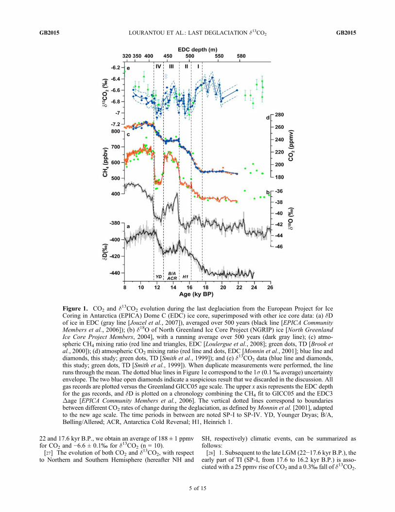
22 and 17.6 kyr B.P., we obtain an average of 188 ± 1 ppmvfor CO2 and −6.6 ± 0.1‰ for d13CO2 (n = 10).[27] The evolution of both CO2 and d13CO2, with respect

to Northern and Southern Hemisphere (hereafter NH and

SH, respectively) climatic events, can be summarized asfollows:[28] 1. Subsequent to the late LGM (22−17.6 kyr B.P.), the

early part of TI (SP‐I, from 17.6 to 16.2 kyr B.P.) is asso-ciated with a 25 ppmv rise of CO2 and a 0.3‰ fall of d13CO2.

Figure 1. CO2 and d13CO2 evolution during the last deglaciation from the European Project for IceCoring in Antarctica (EPICA) Dome C (EDC) ice core, superimposed with other ice core data: (a) dDof ice in EDC (gray line [Jouzel et al., 2007]), averaged over 500 years (black line [EPICA CommunityMembers et al., 2006]); (b) d18O of North Greenland Ice Core Project (NGRIP) ice [North GreenlandIce Core Project Members, 2004], with a running average over 500 years (dark gray line); (c) atmo-spheric CH4 mixing ratio (red line and triangles, EDC [Loulergue et al., 2008]; green dots, TD [Brook etal., 2000]); (d) atmospheric CO2 mixing ratio (red line and dots, EDC [Monnin et al., 2001]; blue line anddiamonds, this study; green dots, TD [Smith et al., 1999]); and (e) d13CO2 data (blue line and diamonds,this study; green dots, TD [Smith et al., 1999]). When duplicate measurements were performed, the lineruns through the mean. The dotted blue lines in Figure 1e correspond to the 1s (0.1‰ average) uncertaintyenvelope. The two blue open diamonds indicate a suspicious result that we discarded in the discussion. Allgas records are plotted versus the Greenland GICC05 age scale. The upper x axis represents the EDC depthfor the gas records, and dD is plotted on a chronology combining the CH4 fit to GICC05 and the EDC3Dage [EPICA Community Members et al., 2006]. The vertical dotted lines correspond to boundariesbetween different CO2 rates of change during the deglaciation, as defined byMonnin et al. [2001], adaptedto the new age scale. The time periods in between are noted SP‐I to SP‐IV. YD, Younger Dryas; B/A,Bølling/Allerød; ACR, Antarctica Cold Reversal; H1, Heinrich 1.


5 of 15

[29] 2. SP‐II (16.2 to 14.7 kyr B.P.), during which theHeinrich 1 (H1) event ends in the NH (as deduced from ice‐rafted debris in the North Atlantic [Hemming, 2004] and alsoseen in NGRIP temperature data in Figure 1b), reveals a two‐step CO2 rise; the first occurs until 15 kyr B.P. with a pro-gressive 14 ppmv increase and the second with a 12 ppmvrise within only 300 years. Meanwhile, d13CO2 experiencesan oscillation of ∼0.2‰ amplitude and reaches a minimum of−7.0 ± 0.1‰ at about 15.5 kyr B.P., followed by a return toheavier values of ∼ −6.8‰. A small d13CO2 peak also takesplace at the start of SP‐II, which coincides with a slightlysmaller rate of CO2 increase in the detailed Monnin et al.[2001] record. In a recent study, Barker et al. [2009]introduced the notion of “Heinrich Stadial 1” to character-ize oceanic conditions during the first two SP; we will referto this notion in the following.[30] 1. SP‐III (from 14.7 to 12.8 kyr B.P.), coincident

with the Antarctic Cold Reversal (ACR) in the SH and theBølling/Allerød (B/A) warm event in the NH, is marked by aprogressive 3 ppmv decrease of CO2, while a positiveexcursion culminating at −6.5 ± 0.1‰ during the mid‐SP‐III(∼14.1 kyr B.P.) is observed for d13CO2.[31] 2. SP‐IV (between 12.8 and 11.6 kyr B.P.), during

which the Younger Dryas (YD) cold event in the NH andthe post‐ACR warming in the SH took place, reveals similarpatterns for both CO2 and d13CO2 as for SP‐II. Thus, a pro-gressive 13 ppmv CO2 increase is observed until 12 kyr B.P.,while a more abrupt rise of 10 ppmv is seen during the last300 years. d13CO2 experiences a negative excursion of morethan 0.2‰ amplitude, down to −7.0 ± 0.1‰ (n = 6).[32] 3. The EH (11.6 to 9 kyr B.P.) d13CO2 mean level is

more 13C‐enriched than during SP‐IV and amounts to −6.8 ±0.1‰ (n = 14). It also seems by 0.2 ± 0.2‰ more depletedin 13C than at the end of LGM. In contrast, previous studiesconcluded to more enriched d13CO2 values during theHolocene (by 0.16‰ in SM1999 to 0.2 ± 0.2‰ [Leuenbergeret al., 1992]) than at the LGM. They were based on mea-surements performed on older LGM ice (Figure 1d), whileHolocene data covered a different time window than con-sidered here (from 9 to 7 kyr B.P., GICC05 age scale; seeFigures 1d and 1e). In addition, the Holocene d13CO2 levelmay be subject to significant fluctuations, as pointed out bySM1999.[33] Our measurements show that, although d13CO2 starts

to decrease in parallel with the early CO2 increase (a trendnot captured in the less resolved SM1999 signal), its rapiddrop takes place ∼1 kyr later, when CO2 has alreadyincreased by more than 10 ppmv. On the other hand, the EHd13CO2 rise appears more modest in our data set than in theTD record.

4. Discussion

[34] Despite the small size of the d13CO2 signal to bedeciphered and the relatively small signal‐to‐noise ratio,some clear conclusions can now be drawn on its evolutionduring TI. Our more detailed EDC d13CO2 signal comparedto the TD one supports some of the earlier conclusionsdrawn by SM1999. It also sheds some new light on the Ccycle dynamics during the last deglaciation. The EDC

record highlights an overall W shape of atmospheric d13CO2

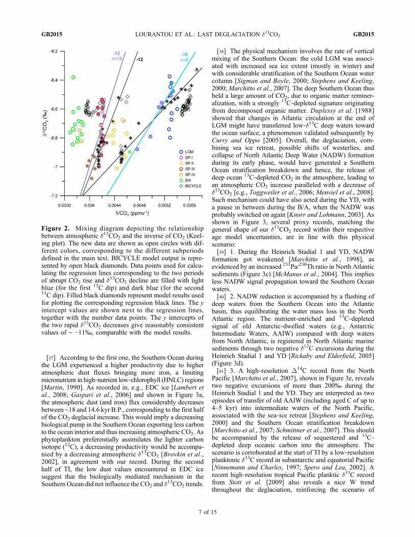
first broadly depicted by the SM1999 record throughout TI.It differs from SM1999 on the following patterns: (1) thetwo well‐resolved minima taking place at times of steadilyand important rises of CO2 levels (late part of H1, and YD)reach comparable d13CO2 levels, around −7.0‰; (2) theCO2 plateau accompanying the ACR goes together with ad13CO2 peak; (3) the average d13CO2 during the EH seemsslightly more 13C‐depleted than at the end of LGM; and(4) SM1999 used a plot of d13CO2 as a function of theinverse of CO2 (a so‐called “Keeling plot,” i.e., a mixingdiagram where the y intercept should provide the isotopiccomposition of the added CO2 in the atmosphere), taking allT‐I data together to discuss the possible cause of the CO2

increase. The improved time resolution of our data set per-mits us to subdivide T‐I with distinct intercepts through time.A y intercept of −6‰ is obtained, similar to all deglacial dataof SM1999, but only through SP‐II and SP‐III data (notshown). On the other hand, the two periods when CO2

largely increases and d13CO2 simultaneously decreases inour record (SP‐I and SP‐IV) reveal another “Keeling plot”type of isotopic signature for the additional CO2, similar forboth subperiods: ∼−11‰ (blue lines of Figure 2). The mainconclusion of SM1999 that the C cycle behaved in a dualmode depending on the speed of climatic changes, i.e., aslow mode taking place during the EH and LGM, and a fastmode during TI, is thus not supported by the new Keelingplot (see Text S1).1

[35] The similar “Keeling plot” signature of SP‐I and SP‐IV suggests at first hand that the two main steps of atmo-spheric CO2 increase during TI involved similar C cyclemechanisms. But their common y intercept cannot bedirectly interpreted as the isotopic signature of such me-chanisms. Keeling plots work well only in an atmosphere‐biosphere two‐reservoir system experiencing fast exchanges[e.g., Pataki et al., 2003]. On timescales of centuries tomillennia such as during TI, the isotopic buffering effect ofthe ocean (air/sea exchanges, carbonate system) modifiesthe y intercept in a three‐reservoir model, as shown forinstance by [Köhler et al., 2006a] using the preindustrial toindustrial CO2 increase and d

13CO2 decrease as a case study.Therefore, other approaches are required to extract possiblescenarios out of our new data set, relevant to carbon ex-changes between the atmosphere, ocean and biosphereduring TI. We use two of them here: a comparison withproxy records relevant to C cycle processes, and simulationsof CO2 and d13CO2 with two C cycle box models.

4.1. Comparison With Other C Cycle Proxy Records

[36] The good correlation between CO2 and Antarcticdeuterium throughout TI (Figures 1a and 1d), alreadynoticed in numerous works [e.g., Monnin et al., 2001;Bianchi and Gersonde, 2004], points toward a leading roleof the Southern Ocean to drive the corresponding CO2

evolution. As pointed out in the introduction, two types ofSouthern Ocean processes, a biological and a physical one,can be evoked.

1Auxiliary material is available with the HTML. doi:10.1029/2009GB003545.


6 of 15

[37] According to the first one, the Southern Ocean duringthe LGM experienced a higher productivity due to higheratmospheric dust fluxes bringing more iron, a limitingmicronutrient in high‐nutrient low‐chlorophyll (HNLC) regions[Martin, 1990]. As recorded in, e.g., EDC ice [Lambert etal., 2008; Gaspari et al., 2006] and shown in Figure 3a,the atmospheric dust (and iron) flux considerably decreasesbetween ∼18 and 14.6 kyr B.P., corresponding to the first halfof the CO2 deglacial increase. This would imply a decreasingbiological pump in the Southern Ocean exporting less carbonto the ocean interior and thus increasing atmospheric CO2. Asphytoplankton preferentially assimilates the lighter carbonisotope (12C), a decreasing productivity would be accompa-nied by a decreasing atmospheric d13CO2 [Brovkin et al.,2002], in agreement with our record. During the secondhalf of TI, the low dust values encountered in EDC icesuggest that the biologically mediated mechanism in theSouthern Ocean did not influence the CO2 and d

13CO2 trends.

[38] The physical mechanism involves the rate of verticalmixing of the Southern Ocean: the cold LGM was associ-ated with increased sea ice extent (mostly in winter) andwith considerable stratification of the Southern Ocean watercolumn [Sigman and Boyle, 2000; Stephens and Keeling,2000; Marchitto et al., 2007]. The deep Southern Ocean thusheld a large amount of CO2, due to organic matter reminer-alization, with a strongly 13C‐depleted signature originatingfrom decomposed organic matter. Duplessy et al. [1988]showed that changes in Atlantic circulation at the end ofLGM might have transferred low‐d13C deep waters towardthe ocean surface, a phenomenon validated subsequently byCurry and Oppo [2005]. Overall, the deglaciation, com-bining sea ice retreat, possible shifts of westerlies, andcollapse of North Atlantic Deep Water (NADW) formationduring its early phase, would have generated a SouthernOcean stratification breakdown and hence, the release ofdeep ocean 13C‐depleted CO2 in the atmosphere, leading toan atmospheric CO2 increase paralleled with a decrease ofd13CO2 [e.g., Toggweiler et al., 2006; Menviel et al., 2008].Such mechanism could have also acted during the YD, witha pause in between during the B/A, when the NADW wasprobably switched on again [Knorr and Lohmann, 2003]. Asshown in Figure 3, several proxy records, matching thegeneral shape of our d13CO2 record within their respectiveage model uncertainties, are in line with this physicalscenario:[39] 1. During the Heinrich Stadial 1 and YD, NADW

formation got weakened [Marchitto et al., 1998], asevidenced by an increased 231Pa/230Th ratio in North Atlanticsediments (Figure 3c) [McManus et al., 2004]. This impliesless NADW signal propagation toward the Southern Oceanwaters.[40] 2. NADW reduction is accompanied by a flushing of

deep waters from the Southern Ocean into the Atlanticbasin, thus equilibrating the water mass loss in the NorthAtlantic region. The nutrient‐enriched and 13C‐depletedsignal of old Antarctic‐dwelled waters (e.g., AntarcticIntermediate Waters, AAIW) compared with deep watersfrom North Atlantic, is registered in North Atlantic marinesediments through two negative d13C excursions during theHeinrich Stadial 1 and YD [Rickaby and Elderfield, 2005](Figure 3d).[41] 3. A high‐resolution D14C record from the North

Pacific [Marchitto et al., 2007], shown in Figure 3e, revealstwo negative excursions of more than 200‰ during theHeinrich Stadial 1 and the YD. They are interpreted as twoepisodes of transfer of old AAIW (including aged C of up to4–5 kyr) into intermediate waters of the North Pacific,associated with the sea‐ice retreat [Stephens and Keeling,2000] and the Southern Ocean stratification breakdown[Marchitto et al., 2007; Schmittner et al., 2007]. This shouldbe accompanied by the release of sequestered and 13C‐depleted deep oceanic carbon into the atmosphere. Thescenario is corroborated at the start of TI by a low‐resolutionplanktonic d13C record in subantarctic and equatorial Pacific[Ninnemann and Charles, 1997; Spero and Lea, 2002]. Arecent high‐resolution tropical Pacific planktic d13C recordfrom Stott et al. [2009] also reveals a nice W trendthroughout the deglaciation, reinforcing the scenario of

Figure 2. Mixing diagram depicting the relationshipbetween atmospheric d13CO2 and the inverse of CO2 (Keel-ing plot). The new data are shown as open circles with dif-ferent colors, corresponding to the different subperiodsdefined in the main text. BICYCLE model output is repre-sented by open black diamonds. Data points used for calcu-lating the regression lines corresponding to the two periodsof abrupt CO2 rise and d13CO2 decline are filled with lightblue (for the first 13C dip) and dark blue (for the second13C dip). Filled black diamonds represent model results usedfor plotting the corresponding regression black lines. The yintercept values are shown next to the regression lines,together with the number data points. The y intercepts ofthe two rapid d13CO2 decreases give reasonably consistentvalues of ∼ −11‰, comparable with the model results.


7 of 15

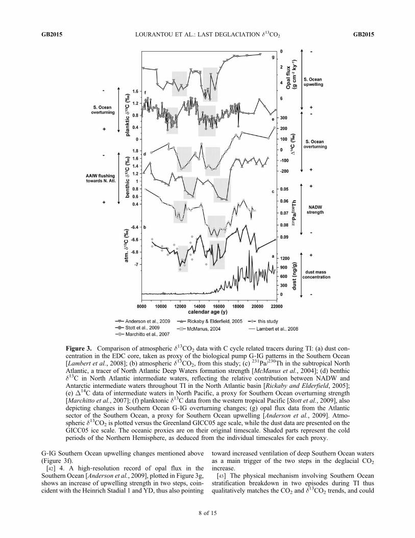
G‐IG Southern Ocean upwelling changes mentioned above(Figure 3f).[42] 4. A high‐resolution record of opal flux in the

Southern Ocean [Anderson et al., 2009], plotted in Figure 3g,shows an increase of upwelling strength in two steps, coin-cident with the Heinrich Stadial 1 and YD, thus also pointing

toward increased ventilation of deep Southern Ocean watersas a main trigger of the two steps in the deglacial CO2

increase.[43] The physical mechanism involving Southern Ocean

stratification breakdown in two episodes during TI thusqualitatively matches the CO2 and d13CO2 trends, and could

Figure 3. Comparison of atmospheric d13CO2 data with C cycle related tracers during TI: (a) dust con-centration in the EDC core, taken as proxy of the biological pump G‐IG patterns in the Southern Ocean[Lambert et al., 2008]; (b) atmospheric d13CO2, from this study; (c) 231Pa/230Th in the subtropical NorthAtlantic, a tracer of North Atlantic Deep Waters formation strength [McManus et al., 2004]; (d) benthicd13C in North Atlantic intermediate waters, reflecting the relative contribution between NADW andAntarctic intermediate waters throughout TI in the North Atlantic basin [Rickaby and Elderfield, 2005];(e) D14C data of intermediate waters in North Pacific, a proxy for Southern Ocean overturning strength[Marchitto et al., 2007]; (f) planktonic d13C data from the western tropical Pacific [Stott et al., 2009], alsodepicting changes in Southern Ocean G‐IG overturning changes; (g) opal flux data from the Atlanticsector of the Southern Ocean, a proxy for Southern Ocean upwelling [Anderson et al., 2009]. Atmo-spheric d13CO2 is plotted versus the Greenland GICC05 age scale, while the dust data are presented on theGICC05 ice scale. The oceanic proxies are on their original timescale. Shaded parts represent the coldperiods of the Northern Hemisphere, as deduced from the individual timescales for each proxy.


8 of 15

also explain the common “Keeling plot” isotopic signatureof the added carbon during the two episodes. Aside from thebiological pump and ocean circulation hypotheses, a possi-bly straightforward explanation of the coevolution betweenCO2 and d13CO2 concerns changes in Sea Surface Tem-perature (SST) during TI: due to isotopic fractionation duringair/sea exchanges, a warmer ocean will leave a 13C‐enrichedsignal in the atmosphere. SM1999 assigned a large portionof their d13CO2 signal to this mechanism, by considering aglobally averaged SST increase of 5°C between the LGMand EH. On the other hand, Brovkin et al. [2002], using theclimate model CLIMBER‐2, pointed out that the parallelchanges of CO2, alkalinity and bicarbonate ion concentra-tion significantly affect the isotopic fractionation during air/sea exchanges, thus reducing the atmospheric d13CO2

imprint of SST changes. Moreover, the rapid d13CO2

changes observed in our record may be difficult to rec-oncile with the speed of SST changes in areas of deep waterformation.[44] SP‐III encounters terrestrial carbon buildup in vege-

tation, soils and peat deposits [MacDonald et al., 2006]which could have contributed to the small CO2 decrease andto a positive d13CO2 anomaly in the atmosphere, as thebiosphere preferentially assimilates 12C. This is qualitativelycorroborated by the CH4 evolution (Figure 1c), pointingtoward a switch‐on of boreal wetland CH4 emissions(requiring a concomitant intensification of the terrestrial Ccycle) at that time [Fischer et al., 2008]. Alternative sce-narios attribute even more control of the d13CO2 variabilityby terrestrial biosphere carbon uptake and release as aconsequence of abrupt temperature changes in the NHcaused by the AMOC shutdown during H1 and YD [e.g.,Köhler et al., 2005b]. For the deglacial CO2 rise, the con-tribution from progressively flooded continental shelvesmight also need some consideration [Montenegro et al.,2006]; however, this scenario is challenged by the lag ofthe sea level increase with respect to CO2 [Pépin et al.,2001].[45] In summary, the qualitative comparison of the EDC

CO2 and d13CO2 records with C cycle proxies suggest adominant role of increased overturning in the SouthernOcean (as mainly evidenced by D14C, opal flux and d13Crecords) during SP‐I and SP‐II to explain the two main stepsof CO2 increase, with an additional contribution of reducedbiological pump during SP‐I. The two mechanisms wouldhave stalled during SP‐III when NADW became stronger,and would also have been counterbalanced by terrestrialcarbon buildup. To go further into a quantitative evaluationof mechanisms able to explain the CO2 and d13CO2 signals,modeling is required. In the following, we explore theproblem using two C cycle box models.

4.2. BICYCLE Model Runs

[46] We employed the BICYCLE model [Köhler et al.,2005a], a coupled atmosphere/ocean/sediment/biosphere Ccycle box model, run in a transient mode and forced withvarious time‐dependent paleoclimatic data over TI. It con-sists of a single atmospheric box interacting with a 10 boxocean reservoir and the terrestrial biosphere, which is sub-divided into seven compartments [Köhler et al., 2005a]. The

ocean further communicates with a sediment reservoir. Massbalance equations are solved for the carbon stocks of thebiospheric compartments, for DIC, TAlk, PO4 and O2 in the10 oceanic reservoirs, for CO2 in the atmosphere and forthe carbon isotopes in all reservoirs.[47] BICYCLE is the only C cycle model we are aware of

which was run in transient mode over TI. It was also usedfor the interpretation of atmospheric carbon records anddeep ocean d13C data over TI and much longer timescales ofup to 2 Myr [Köhler et al., 2005a, 2006a, 2006b; Köhlerand Fischer, 2006; Köhler and Bintanja, 2008; Köhler etal., 2010]. Since its application over TI [Köhler et al.,2005a], improvements were performed in the parameteri-zation of ocean circulation and sediment‐ocean interaction,we thus use new simulation results, instead of the modeloutput published by Köhler et al. [2005a].4.2.1. Parameterizations[48] The main model parameterizations, based on data

obtained from ice core or marine cores (Figure 4) are thefollowing:[49] 1. Sea level rises by ∼110m between 22 and 8 kyr B.P.

based on reconstructions of coral reef terraces [Fairbanks,1989] (Figure 4a). This leads to changes in the salinity, inthe concentrations of all oceanic tracers and in the volumes ofthe oceanic boxes.[50] 2. Temperature of all oceanic boxes is prescribed for

present day from Levitus and Boyer [1994]. It changes overtime according to oceanic proxy evidences for equatorialSST [Visser et al., 2003] and deep ocean temperature[Labeyrie et al., 1987] (Figure 4c). At high latitudes, it isrepresented by ice core isotopic profiles (North Atlanticand North Pacific: d18O on GICC05 age scale from North-GRIP [North Greenland Ice Core Project Members, 2004;Andersen et al., 2007] (Figure 4b); Southern Ocean: dD(corrected for the effect of sea level rise) from EDC[Parrenin et al., 2007; Jouzel et al., 2001] synchronized toGICC05 [EPICACommunityMembers et al., 2006;Andersenet al., 2007], as shown in Figure 4d. Both ice core recordsare scaled to provide a SST DT of 4 K between the mini-mum glacial values and the present day.[51] 3. Marine productivity in the Southern Ocean is

scaled (if allowed by macronutrient availability) on dustinput to the Southern Ocean as approximated by the nonsea‐salt‐dust record measured in EDC [Roethlisberger et al.,2002] (Figure 4e).[52] 4. Ocean circulation between the 10 boxes for present

conditions is parameterized with data from the World OceanCirculation Experiment WOCE [Ganachaud and Wunsch,2000] (Figure 4f). Compared to the initial BICYCLE runsover TI [Köhler et al., 2005a], it was slightly modified to geta better agreement between simulated and reconstructedoceanic 13C [Köhler et al., 2010]. About 30% of theupwelled waters in the Southern Ocean are immediatelyredistributed to the intermediate equatorial Atlantic Ocean toaccount for the effect that, in the natural carbon cycle,upwelling waters in the Southern Ocean (which are thenflowing as water masses of intermediate depth to the north)are still enriched in DIC [Gruber et al., 2009]. Three majorocean currents are parameterized as follows (Figure 4f):(1) The strength of NADW (i.e., of its overturning [cf.


9 of 15

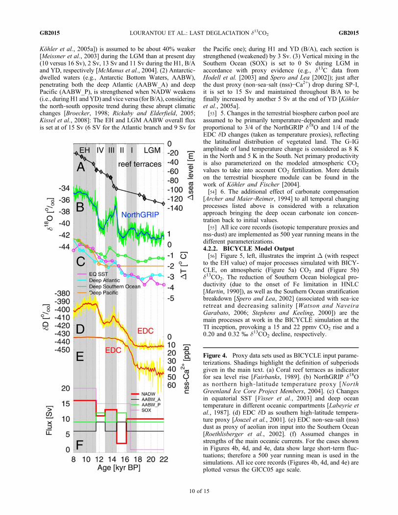
Köhler et al., 2005a]) is assumed to be about 40% weaker[Meissner et al., 2003] during the LGM than at present day(10 versus 16 Sv), 2 Sv, 13 Sv and 11 Sv during the H1, B/Aand YD, respectively [McManus et al., 2004]. (2) Antarctic‐dwelled waters (e.g., Antarctic Bottom Waters, AABW),penetrating both the deep Atlantic (AABW_A) and deepPacific (AABW_P), is strengthened when NADW weakens(i.e., duringH1 andYD) and vice versa (for B/A), consideringthe north‐south opposite trend during these abrupt climaticchanges [Broecker, 1998; Rickaby and Elderfield, 2005;Kissel et al., 2008]: The EH and LGM AABW overall fluxis set at of 15 Sv (6 SV for the Atlantic branch and 9 Sv for

the Pacific one); during H1 and YD (B/A), each section isstrengthened (weakened) by 3 Sv. (3) Vertical mixing in theSouthern Ocean (SOX) is set to 0 Sv during LGM inaccordance with proxy evidence (e.g., d13C data fromHodell et al. [2003] and Spero and Lea [2002]); just afterthe dust proxy (non‐sea‐salt (nss)−Ca2+) drop during SP‐I,it is set to 15 Sv and maintained throughout B/A to befinally increased by another 5 Sv at the end of YD [Köhleret al., 2005a].[53] 5. Changes in the terrestrial biosphere carbon pool are

assumed to be primarily temperature‐dependent and madeproportional to 3/4 of the NorthGRIP d18O and 1/4 of theEDC dD changes (taken as temperature proxies), reflectingthe latitudinal distribution of vegetated land. The G‐IGamplitude of land temperature change is considered as 8 Kin the North and 5 K in the South. Net primary productivityis also parameterized on the modeled atmospheric CO2

values to take into account CO2 fertilization. More detailson the terrestrial biosphere module can be found in thework of Köhler and Fischer [2004].[54] 6. The additional effect of carbonate compensation

[Archer and Maier‐Reimer, 1994] to all temporal changingprocesses listed above is considered with a relaxationapproach bringing the deep ocean carbonate ion concen-tration back to initial values.[55] All ice core records (isotopic temperature proxies and

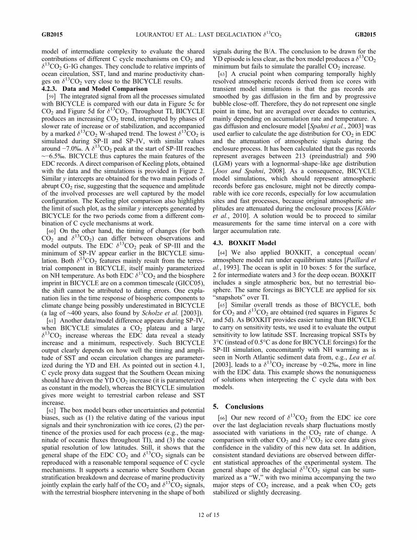
nss‐dust) are implemented as 500 year running means in thedifferent parameterizations.4.2.2. BICYCLE Model Output[56] Figure 5, left, illustrates the imprint D (with respect

to the EH value) of major processes simulated with BICY-CLE, on atmospheric (Figure 5a) CO2 and (Figure 5b)d13CO2. The reduction of Southern Ocean biological pro-ductivity (due to the onset of Fe limitation in HNLC[Martin, 1990]), as well as the Southern Ocean stratificationbreakdown [Spero and Lea, 2002] (associated with sea‐iceretreat and decreasing salinity [Watson and NaveiraGarabato, 2006; Stephens and Keeling, 2000]) are themain processes at work in the BICYCLE simulation at theTI inception, provoking a 15 and 22 ppmv CO2 rise and a0.20 and 0.32 ‰ d13CO2 decline, respectively.

Figure 4. Proxy data sets used as BICYCLE input parame-terizations. Shadings highlight the definition of subperiodsgiven in the main text. (a) Coral reef terraces as indicatorfor sea level rise [Fairbanks, 1989]. (b) NorthGRIP d18Oas northern high‐latitude temperature proxy [NorthGreenland Ice Core Project Members, 2004]. (c) Changesin equatorial SST [Visser et al., 2003] and deep oceantemperature in different oceanic compartments [Labeyrie etal., 1987]. (d) EDC dD as southern high‐latitude tempera-ture proxy [Jouzel et al., 2001]. (e) EDC non‐sea‐salt (nss)dust as proxy of aeolian iron input into the Southern Ocean[Roethlisberger et al., 2002]. (f) Assumed changes instrengths of the main oceanic currents. For the cases shownin Figures 4b, 4d, and 4e, data show large short‐term fluc-tuations; therefore a 500 year running mean is used in thesimulations. All ice core records (Figures 4b, 4d, and 4e) areplotted versus the GICC05 age scale.


10 of 15

[57] During the NH cold events (H1 and YD), NADWweakens [McManus et al., 2004], dampening the CO2 increaseand d13CO2 decrease related to AABW enhancement(+4.5 ppmv; −0.04‰) [Rickaby and Elderfield, 2005];NADW (AABW) strengthening (weakening) at the end ofSP‐II and SP‐IV, combined with stronger Southern Oceanwater mixing at the end of YD, lead to a CO2 outgassing of10 and 7 ppmv, respectively (see Text S1).[58] Sea level rise [Fairbanks, 1989] processes do not

leave an important imprint on d13CO2 within the SPs,although they significantly affect CO2 during the ACR, byprovoking a 3 ppmv reduction (see Text S1). In contrast,vegetation growth, lagging SouthernOceanwarming [Hughenet al., 2004] and forced by CO2 fertilization and NHwarming, starts affecting d13CO2 during SP‐II and becomesa major driver of this signal during SP‐III and SP‐IV (green

line of Figures 5a and 5b). The rise and fall of total bio-spheric carbon by 200PgC during SP‐III and SP‐IV,respectively [Köhler and Fischer, 2004; Köhler et al.,2005a], lead to a 15 ppmv decrease and a 17 ppmv rise ofCO2, also causing a +0.35‰ and −0.40‰ d13CO2 anomaly.The response of atmospheric CO2 to terrestrial C change isin corroboration with previous numerical studies: forexample [Scholze et al., 2003], assuming a total 180 PgCdecline of terrestrial carbon pools during YD results in anatmospheric CO2 rise of 30 ppmv due to land cooling andprecipitation decline, both following the overturning circu-lation reduction. Köhler et al. [2005b] find, as a conse-quence of the AMOC shutdown and the accompanyingNorthern Hemispheric cooling, a total decline of terrestrialcarbon pools of up to 140 PgC, resulting in peak‐to‐peakchanges in atmospheric CO2 and d13CO2 of 13 ppmv and0.25‰, respectively. Recently, Brovkin et al. [2007] used a

Figure 5. Comparison between EDC CO2 and d13CO2 data and box model simulations. (left) Imprint ofindividual major C cycle processes on atmospheric (a) CO2 and (b) d

13CO2, simulated with the BICYCLEmodel. All curves express an anomalyDpCO2 andDd13CO2 versus a reference corresponding to boundaryEH conditions. The following processes are shown at this point: (1) Southern Ocean mixing; (2) marineproductivity; (3) ocean temperature; and (4) terrestrial biosphere. (right) Superposition of the BICYCLEsimulation integrating all individual processes of Figure 5 (left) (gray line) with our data (deep blue lineand diamonds). The equilibrium‐state BOXKIT model outputs, using similar boundary conditions asBICYCLE for each time period (red triangles) are also plotted for (c) CO2 and (d) d13CO2. Red squarescorrespond to BOXKIT simulations using higher equatorial SST magnitudes. All series are plotted versusGICC05 age scale.


11 of 15

model of intermediate complexity to evaluate the sharedcontributions of different C cycle mechanisms on CO2 andd13CO2 G‐IG changes. They conclude to relative imprints ofocean circulation, SST, land and marine productivity chan-ges on d13CO2 very close to the BICYCLE results.4.2.3. Data and Model Comparison[59] The integrated signal from all the processes simulated

with BICYCLE is compared with our data in Figure 5c forCO2 and Figure 5d for d13CO2. Throughout TI, BICYCLEproduces an increasing CO2 trend, interrupted by phases ofslower rate of increase or of stabilization, and accompaniedby a marked d13CO2 W‐shaped trend. The lowest d13CO2 issimulated during SP‐II and SP‐IV, with similar valuesaround −7.0‰. A d13CO2 peak at the start of SP‐III reaches∼−6.5‰. BICYCLE thus captures the main features of theEDC records. A direct comparison of Keeling plots, obtainedwith the data and the simulations is provided in Figure 2.Similar y intercepts are obtained for the two main periods ofabrupt CO2 rise, suggesting that the sequence and amplitudeof the involved processes are well captured by the modelconfiguration. The Keeling plot comparison also highlightsthe limit of such plot, as the similar y intercepts generated byBICYCLE for the two periods come from a different com-bination of C cycle mechanisms at work.[60] On the other hand, the timing of changes (for both

CO2 and d13CO2) can differ between observations andmodel outputs. The EDC d13CO2 peak of SP‐III and theminimum of SP‐IV appear earlier in the BICYCLE simu-lation. Both d13CO2 features mainly result from the terres-trial component in BICYCLE, itself mainly parameterizedon NH temperature. As both EDC d13CO2 and the biosphereimprint in BICYCLE are on a common timescale (GICC05),the shift cannot be attributed to dating errors. One expla-nation lies in the time response of biospheric components toclimate change being possibly underestimated in BICYCLE(a lag of ∼400 years, also found by Scholze et al. [2003]).[61] Another data/model difference appears during SP‐IV,

when BICYCLE simulates a CO2 plateau and a larged13CO2 increase whereas the EDC data reveal a steadyincrease and a minimum, respectively. Such BICYCLEoutput clearly depends on how well the timing and ampli-tude of SST and ocean circulation changes are parameter-ized during the YD and EH. As pointed out in section 4.1,C cycle proxy data suggest that the Southern Ocean mixingshould have driven the YD CO2 increase (it is parameterizedas constant in the model), whereas the BICYCLE simulationgives more weight to terrestrial carbon release and SSTincrease.[62] The box model bears other uncertainties and potential

biases, such as (1) the relative dating of the various inputsignals and their synchronization with ice cores, (2) the per-tinence of the proxies used for each process (e.g., the mag-nitude of oceanic fluxes throughout TI), and (3) the coarsespatial resolution of low latitudes. Still, it shows that thegeneral shape of the EDC CO2 and d13CO2 signals can bereproduced with a reasonable temporal sequence of C cyclemechanisms. It supports a scenario where Southern Oceanstratification breakdown and decrease of marine productivityjointly explain the early half of the CO2 and d13CO2 signals,with the terrestrial biosphere intervening in the shape of both

signals during the B/A. The conclusion to be drawn for theYD episode is less clear, as the box model produces a d13CO2

minimum but fails to simulate the parallel CO2 increase.[63] A crucial point when comparing temporally highly

resolved atmospheric records derived from ice cores withtransient model simulations is that the gas records aresmoothed by gas diffusion in the firn and by progressivebubble close‐off. Therefore, they do not represent one singlepoint in time, but are averaged over decades to centuries,mainly depending on accumulation rate and temperature. Agas diffusion and enclosure model [Spahni et al., 2003] wasused earlier to calculate the age distribution for CO2 in EDCand the attenuation of atmospheric signals during theenclosure process. It has been calculated that the gas recordsrepresent averages between 213 (preindustrial) and 590(LGM) years with a lognormal‐shape‐like age distribution[Joos and Spahni, 2008]. As a consequence, BICYCLEmodel simulations, which should represent atmosphericrecords before gas enclosure, might not be directly compa-rable with ice core records, especially for low accumulationsites and fast processes, because original atmospheric am-plitudes are attenuated during the enclosure process [Köhleret al., 2010]. A solution would be to proceed to similarmeasurements for the same time interval on a core withlarger accumulation rate.

4.3. BOXKIT Model

[64] We also applied BOXKIT, a conceptual ocean/atmosphere model run under equilibrium states [Paillard etal., 1993]. The ocean is split in 10 boxes: 5 for the surface,2 for intermediate waters and 3 for the deep ocean. BOXKITincludes a single atmospheric box, but no terrestrial bio-sphere. The same forcings as BICYCLE are applied for six“snapshots” over TI.[65] Similar overall trends as those of BICYCLE, both

for CO2 and d13CO2 are obtained (red squares in Figures 5cand 5d). As BOXKIT provides easier tuning than BICYCLEto carry on sensitivity tests, we used it to evaluate the outputsensitivity to low latitude SST. Increasing tropical SSTs by3°C (instead of 0.5°C as done for BICYCLE forcings) for theSP‐III simulation, concomitantly with NH warming as isseen in North Atlantic sediment data from, e.g., Lea et al.[2003], leads to a d13CO2 increase by ∼0.2‰, more in linewith the EDC data. This example shows the nonuniquenessof solutions when interpreting the C cycle data with boxmodels.

5. Conclusions

[66] Our new record of d13CO2 from the EDC ice coreover the last deglaciation reveals sharp fluctuations mostlyassociated with variations in the CO2 rate of change. Acomparison with other CO2 and d13CO2 ice core data givesconfidence in the validity of this new data set. In addition,consistent standard deviations are observed between differ-ent statistical approaches of the experimental system. Thegeneral shape of the deglacial d13CO2 signal can be sum-marized as a “W,” with two minima accompanying the twomajor steps of CO2 increase, and a peak when CO2 getsstabilized or slightly decreasing.


12 of 15

[67] The comparison with C cycle related proxies high-lights similarities with marine signals associated with thestrength of Southern Ocean ventilation and upwelling,suggesting that this physical mechanism would be the maindriver of the deglacial CO2 increase.[68] Two C cycle box models (BICYCLE and BOXKIT),

run under the same input parameters support the dominantrole of Southern Ocean physical processes and add the marineproductivity decline during the early part of the deglaciationas another mechanism contributing to the d13CO2 decreaseand CO2 increase. The BICYCLE model supports an addi-tional role of terrestrial carbon buildup to explain the CO2

plateau and d13CO2 peak paralleling the ACR. It also simu-lates an early YD d13CO2 minimum followed by an increaseto EH values, attributed to terrestrial carbon and SST decreaseand subsequent increase, an explanation conflicting with Ccycle proxy data which suggest a dominant role of strength-ening Southern Ocean ventilation. The failure of BICYCLEto simulate a parallel CO2 increase shows the limit of thismodeling exercise, which crucially depends on assumptionsregarding SO upwelling changes.[69] More sophisticated approaches using coupled car-

bon‐climate Earth system models will be needed in thefuture to better disentangle the contribution of each process,with their direct parameterizations in the models instead ofthe use of proxies. Our detailed EDC profile clearly high-lights the need for fine time resolution in producing futured13CO2 records throughout major climatic events.

[70] Acknowledgments. This work is a contribution to the EuropeanProject for Ice Coring in Antarctica (EPICA), a joint European ScienceFoundation (ESF)/EC scientific program, funded by the European Com-mission and by national contributions from Belgium, Denmark, France,Germany, Italy, the Netherlands, Norway, Sweden, Switzerland, and theUnited Kingdom. The main logistic support was provided by IPEV andPNRA (at Dome C). A.L. was funded by the European Research Trainingand Mobility Network GREENCYCLES. Additional funding support wasprovided by the QUEST‐INSU project DESIRE, the FP6 STREP EPICA‐MIS, and the French ANR PICC (ANR‐05‐BLAN‐0312‐01). Long‐termsupport for the mass spectrometry work at LGGE was provided by theFondation de France and the Balzan Price. Discussions with G. Dreyfus,H. Schaefer, and G. Delaygue were very much appreciated. We particularlythank C. Lorius for his confidence in our earlier work and five anonymousreviewers for fruitful comments on previous versions of this manuscript.This is EPICA publication 249.

References

Ahn, J., M. Wahlen, B. L. Deck, E. J. Brook, P. A. Mayewski, K. C. Taylor,and J. W. C. White (2004), A record of atmospheric CO2 during the last40,000 years from the Siple Dome, Antarctica ice core, J. Geophys. Res.,109, D13305, doi:10.1029/2003JD004415.

Andersen, K. K., et al. (2007), The Greenland ice core chronology 2005,15–42 ka. Part 1: Constructing the time scale, Quat. Sci. Rev.,25(23–24), 3246–3257.

Anderson, R. F., S. Ali, L. I. Bradtmiller, S. H. H. Nielsen, M. Q. Fleisher,B. E. Anderson, and L. H. Burckle (2009), Wind‐driven upwelling inthe Southern Ocean and the deglacial rise in atmospheric CO2, Science,323(5920), 1443–1448, doi:10.1126/science.1167441.

Anklin, M., J.‐M. Barnola, J. Schwander, B. Stauffer, and D. Raynaud(1995), Processes affecting the CO2 concentrations measured in Green-land ice, Tellus, Ser. B, 47, 461–470.

Archer, D., and E. Maier‐Reimer (1994), Effect of deep‐sea sedimen-tary calcite preservation on atmospheric CO2 concentration, Nature,367(6460), 260–263, doi:10.1038/367260a0.

Archer, D., A. Winguth, D. Lea, and N. Mahowald (2000), What causedthe glacial/interglacial atmospheric pCO2 cycles? Rev. Geophys., 38(2),159–189, doi:10.1029/1999RG000066.

Barker, S., P. Diz, M. J. Vautravers, J. Pike, G. Knorr, I. R. Hall, and W. S.Broecker (2009), Interhemispheric Atlantic seesaw response duringthe last deglaciation, Nature, 457(7233), 1097–1102, doi:10.1038/nature07770.

Bereiter, B., J. Schwander, D. Lüthi, and T. F. Stocker (2009), Change inCO2 concentration and O2/N2 ratio in ice cores due to molecular diffu-sion, Geophys. Res. Lett., 36, L05703, doi:10.1029/2008GL036737.

Bianchi, C., and R. Gersonde (2004), Climate evolution at the last deglaci-ation: The role of the Southern Ocean, Earth Planet. Sci. Lett., 228(3–4),407–424, doi:10.1016/j.epsl.2004.10.003.

Broecker, W. S. (1998), Paleocean circulation during the last deglaciation:A bipolar seesaw?, Paleoceanography, 13(2), 119–121, doi:10.1029/97PA03707.

Broecker, W. S., and T. H. Peng (1986), Carbon cycle: 1985 glacial tointerglacial changes in the operation of the global carbon cycle, Radio-carbon, 28(2A), 309–327.

Brook, E. J., S. Harder, J. Severinghaus, E. J. Steig, and C. M. Sucher(2000), On the origin and timing of rapid changes in atmospheric meth-ane during the last glacial period, Global Biogeochem. Cycles, 14(2),559–572, doi:10.1029/1999GB001182.

Brovkin, V., M. Hofmann, J. Bendtsen, and A. Ganopolski (2002), Oceanbiology could control atmospheric d13C during glacial‐interglacial cycle,Geochem. Geophys. Geosyst., 3(5), 1027, doi:10.1029/2001GC000270.

Brovkin, V., A. Ganopolski, D. Archer, and S. Rahmstorf (2007), Loweringof glacial atmospheric CO2 in response to changes in oceanic circulationand marine biogeochemistry, Paleoceanography, 22, PA4202,doi:10.1029/2006PA001380.

Craig, H., Y. Horibe, and T. Sowers (1988), Gravitational separation ofgases and isotopes in polar ice caps, Science, 242(4886), 1675–1678,doi:10.1126/science.242.4886.1675.

Curry, W. B., and D. W. Oppo (2005), Glacial water mass geometry andthe distribution of d13C of SCO2 in the western Atlantic Ocean, Paleo-ceanography, 20, PA1017, doi:10.1029/2004PA001021.

Dreyfus, G., J. Jouzel, M. L. Bender, A. Landais, V. Masson‐Delmotte, andM. Leuenberger (2010), Firn processes and d15N: Potential for a gas‐phase climate proxy, Quat. Sci. Rev., 29, 28–42.

Duplessy, J. C., N. J. Shackleton, R. G. Fairbanks, L. Labeyrie, D. Oppo,and N. Kallel (1988), Deepwater source variations during the last cli-matic cycle and their impact on the global deepwater circulation, Paleo-ceanography, 3(3), 343–360, doi:10.1029/PA003i003p00343.

EPICA Community Members, et al. (2006), One‐to‐one coupling of glacialclimate variability in Greenland and Antarctica, Nature, 444(7116), 195–198, doi:10.1038/nature05301.

Etheridge, D. M., L. P. Steele, R. L. Langenfelds, R. J. Francey, J.‐M.Barnola, and V. I. Morgan (1996), Natural and anthropogenic changes inatmospheric CO2 over the last 1000 years from air in Antarctic ice andfirn, J. Geophys. Res., 101(D2), 4115–4128, doi:10.1029/95JD03410.

Fairbanks, R. G. (1989), A 17,000‐year glacio‐eustatic sea level record:Influence of glacial melting rates on the Younger Dryas event anddeep‐ocean circulation, Nature, 342(6250), 637–642, doi:10.1038/342637a0.

Ferretti, D. F., D. C. Lowe, R. J. Martin, and G. W. Brailsford (2000), Anew gas chromatograph‐isotope ratio mass spectrometry technique forhigh‐precision, N2O‐free analysis of d13C and d18O in atmosphericCO2 from small air samples, J. Geophys. Res., 105(D5), 6709–6718,doi:10.1029/1999JD901051.

Fischer, H., et al. (2008), Changing boreal methane sources and con-stant biomass burning during the last termination, Nature, 452(7189),864–867, doi:10.1038/nature06825.

Flückiger, J., A. Dällenbach, T. Blunier, B. Stauffer, T. F. Stocker,D. Raynaud, and J.‐M. Barnola (1999), Variations in atmospheric N2Oconcentration during abrupt climatic changes, Science, 285(5425),227–230, doi:10.1126/science.285.5425.227.

Francey, R. J., C. E. Allison, D. M. Etheridge, C. M. Trudinger, I. G. Enting,M. Leuenberger, R. L. Langenfelds, E. Michel, and L. P. Steele (1999),A 1000‐year high precision record of d13C in atmospheric CO2, Tellus,Ser. B, 51(2), 170–193, doi:10.1034/j.1600-0889.1999.t01-1-00005.x.

Friedli, H., H. Lötscher, H. Oeschger, U. Siegenthaler, and B. Stauffer(1986), Ice core record of the 13C/12C ratio of atmospheric CO2 in thepast two centuries, Nature, 324(6094), 237–238, doi:10.1038/324237a0.

Ganachaud, A., and C. Wunsch (2000), Improved estimates of global oceancirculation, heat transport and mixing from hydrographic data, Nature,408(6811), 453–457, doi:10.1038/35044048.


13 of 15

Gaspari, V., C. Barbante, G. Cozzi, P. Cescon, C. F. Boutron, P. Gabrielli,G. Capodaglio, C. Ferrari, J. R. Petit, and B. Delmonte (2006), Atmo-spheric iron fluxes over the last deglaciation: Climatic implications,Geophys. Res. Lett., 33, L03704, doi:10.1029/2005GL024352.

Grachev, A. M., and J. P. Severinghaus (2003), Laboratory determinationof thermal diffusion constants for 29N2/

28N2 in air at temperatures from−60 to 0 °C for reconstruction of magnitudes of abrupt climate changesusing the ice core fossil‐air paleothermometer, Geochim. Cosmochim.Acta, 67(3), 345–360, doi:10.1016/S0016-7037(02)01115-8.

Gruber, N., et al. (2009), Oceanic sources, sinks and transport of atmo-spheric CO2, Global Biogeochem. Cycles, 23, GB1005, doi:10.1029/2008GB003349.

Hemming, S. R. (2004), Heinrich events: Massive late Pleistocene detrituslayers of the North Atlantic and their global climate imprint, Rev. Geo-phys., 42, RG1005, doi:10.1029/2003RG000128.

Hodell, D. A., K. A. Venz, C. D. Charles, and U. S. Ninnemann (2003),Pleistocene vertical carbon isotope and carbonate gradients in the SouthAtlantic sector of the Southern Ocean. Geochem. Geophys. Geosyst., 4(1),1004, doi:10.1029/2002GC000367.

Hughen, K. A., T. I. Eglinton, L. Xu, and M. Makou (2004), Abrupt trop-ical vegetation response to rapid climate changes, Science, 304(5679),1955–1959, doi:10.1126/science.1092995.

Intergovernmental Panel on Climate Change (2007), Climate Change 2007:The Physical Science Basis. Contribution of Working Group I to theFourth Assessment Report of the Intergovernmental Panel on ClimateChange, edited by S. Solomon et al., Cambridge Univ. Press, Cambridge,U. K.

Joos, F., and R. Spahni (2008), Rates of change in natural and anthropo-genic radiative forcing over the past 20,000 years, Proc. Natl. Acad.Sci. U. S. A., 105(5), 1425–1430, doi:10.1073/pnas.0707386105.

Jouzel, J., et al. (2001), A new 27 ky high resolution east Antarctic climaterecord, Geophys. Res. Lett., 28(16), 3199–3202, doi:10.1029/2000GL012243.

Jouzel, J., et al. (2007), Orbital and millennial Antarctic climate variabilityover the past 800,000 years, Science, 317(5839), 793–796, doi:10.1126/science.1141038.

Kissel, C., C. Laj, A. M. Piotrowski, S. L. Goldstein, and S. R. Hemming(2008), Millennial‐scale propagation of Atlantic deep waters to the gla-cial Southern Ocean, Paleoceanography, 23, PA2102, doi:10.1029/2008PA001624.

Knorr, G., and G. Lohmann (2003), Southern Ocean origin for resumptionof Atlantic thermohaline circulation during deglaciation, Nature, 424,532–536, doi:10.1038/nature01855.

Köhler, P., and R. Bintanja (2008), The carbon cycle during the mid Pleis-tocene transition: The Southern Ocean decoupling hypothesis, Clim.Past, 4, 311–332.

Köhler, P., and H. Fischer (2004), Simulating changes in the terrestrial bio-sphere during the last glacial/interglacial transition, Global Planet.Change, 43(1–2), 33–55, doi:10.1016/j.gloplacha.2004.02.005.

Köhler, P., and H. Fischer (2006), Simulating low frequency changes inatmospheric CO2 during the last 740,000 years, Clim. Past, 2(2), 57–78.

Köhler, P., H. Fischer, G. Munhoven, and R. E. Zeebe (2005a), Quantita-tive interpretation of atmospheric carbon records over the last glacial ter-mination, Global Biogeochem. Cycles, 19, GB4020, doi:10.1029/2004GB002345.

Köhler, P., F. Joos, S. Gerber, and R. Knutti (2005b), Simulated changes invegetation distribution, land carbon storage, and atmospheric CO2 inresponse to a collapse of the North Atlantic thermohaline circulation,Clim. Dyn., 25, 689–708, doi:10.1007/s00382-005-0058-8.

Köhler, P., H. Fischer, J. Schmitt, and G. Munhoven (2006a), On the appli-cation and interpretation of Keeling plots in paleo climate research‐deci-phering d13C of atmospheric CO2 measured in ice cores, Biogeosciences,3, 539–556.

Köhler, P., R. Muscheler, and H. Fischer (2006b), A model‐based interpre-tation of low‐frequency changes in the carbon cycle during the last120,000 years and its implications for the reconstruction of atmosphericD14C, Geochem. Geophys. Geosyst., 7, Q11N06, doi:10.1029/2005GC001228.

Köhler, P., H. Fischer, and J. Schmitt (2010), Atmospheric d13CO2 and itsrelation to pCO2 and deep ocean d13C during the last Pleistocene, Paleo-ceanography, 25, PA1213, doi:10.1029/2008PA001703.

Labeyrie, L. D., J. C. Duplessy, and P. L. Blanc (1987), Variations in modeof formation and temperature of oceanic deep waters over the past125,000 years, Nature, 327(6122), 477–482, doi:10.1038/327477a0.

Lambert, F., B. Delmonte, J. R. Petit, M. Bigler, P. R. Kaufmann, M. A.Hutterli, T. F. Stocker, U. Ruth, J. P. Steffensen, and V. Maggi(2008), Dust‐climate couplings over the past 800,000 years from the

EPICA Dome C ice core, Nature, 452(7187), 616–619, doi:10.1038/nature06763.

Lea, D. W., D. K. Pak, L. C. Peterson, and K. A. Hughen (2003), Syn-chroneity of tropical and high‐latitude Atlantic temperatures over thelast glacial termination, Science, 301(5638), 1361–1364, doi:10.1126/science.1088470.

Leuenberger, M., U. Siegenthaler, and C. C. Langway (1992), Carbon iso-tope composition of atmospheric CO2 during the last ice age from anAntarctic ice core, Nature, 357(6378), 488–490, doi:10.1038/357488a0.

Levitus, S., and T. P. Boyer (1994), World Ocean Atlas, vol. 4, Tempera-ture, NOAA Atlas NESDIS 4, 117 pp., U.S. Dept. of Comm., Washington,D. C.

Loulergue, L., F. Parrenin, T. Blunier, J.‐M. Barnola, R. Spahni, A. Schilt,G. Raisbeck, and J. Chappellaz (2007), New constraints on the gas age‐ice age difference along the EPICA ice cores, 0–50 kyr, Clim. Past, 3(3),527–540.

Loulergue, L., A. Schilt, R. Spahni, V. Masson‐Delmotte, T. Blunier,B. Lemieux, J.‐M. Barnola, D. Raynaud, T. F. Stocker, and J. Chappellaz(2008), Orbital and millennial‐scale features of atmospheric CH4 overthe past 800,000 years, Nature, 453(7193), 383–386, doi:10.1038/nature06950.

Lourantou, A. (2009), Constraints on the carbon dioxide deglacial risebased on its stable carbon isotopic ratio, Ph.D. thesis, 194 pp., Univ.Joseph Fourier, Grenoble, France.

MacDonald, G. M., D. W. Beilman, K. V. Kremenetski, Y. Sheng, L. C.Smith, and A. A. Velichko (2006), Rapid early development of circu-marctic peatlands and atmospheric CH4 and CO2 variations, Science,314(5797), 285–288, doi:10.1126/science.1131722.

Marchitto, J. T. M., W. B. Curry, and D. W. Oppo (1998), Millennial‐scalechanges in North Atlantic circulation since the last glaciation, Nature,393(6685), 557–561, doi:10.1038/31197.

Marchitto, T. M., S. J. Lehman, J. D. Ortiz, J. Flückiger, and A. van Geen(2007), Marine radiocarbon evidence for the mechanism of deglacialatmospheric CO2 rise, Science, 316(5830), 1456–1459, doi:10.1126/sci-ence.1138679.

Martin, J. H. (1990), Glacial‐interglacial CO2 change: The iron hypothesis,Paleoceanography, 5(1), 1–13, doi:10.1029/PA005i001p00001.

McManus, J. F., R. Francois, J.‐M. Gherardi, L. D. Keigwin, andS. Brown‐Leger (2004), Collapse and rapid resumption of Atlantic merid-ional circulation linked to deglacial climate changes, Nature, 428(6985),834–837, doi:10.1038/nature02494.

Meissner, K. J., A. Schmittner, A. J. Weaver, and J. F. Adkins (2003), Ven-tilation of the North Atlantic Ocean during the Last Glacial Maximum: Acomparison between simulated and observed radiocarbon ages, Paleo-ceanography, 18(2), 1023, doi:10.1029/2002PA000762.

Menviel, L., A. Timmermann, A. Mouchet, and O. Timm (2008), Climateand marine carbon cycle response to changes in the strength of the South-ernHemispheric westerlies,Paleoceanography, 23, PA4201, doi:10.1029/2008PA001604.

Monnin, E., A. Indermühle, A. Dällenbach, J. Flückiger, B. Stauffer,T. F. Stocker, D. Raynaud, and J.‐M. Barnola (2001), Atmospheric CO2concentrations over the last glacial Termination, Science, 291(5501),112–114, doi:10.1126/science.291.5501.112.

Montenegro, A., M. Eby, J. O. Kaplan, K. J. Meissner, and A. J. Weaver(2006), Carbon storage on exposed continental shelves during theglacial‐interglacial transition, Geophys. Res. Lett., 33, L08703,doi:10.1029/2005GL025480.

North Greenland Ice Core Project Members (2004), High‐resolution recordof Northern Hemisphere climate extending into the last interglacialperiod, Nature, 431(7005), 147–151, doi:10.1038/nature02805.

Ninnemann, U. S., and C. D. Charles (1997), Regional differences inQuaternary subantarctic nutrient cycling: Link to intermediate and deepwater ventilation, Paleoceanography, 12(4), 560–567, doi:10.1029/97PA01032.

Obata, A. (2007), Climate carbon cycle model response to freshwater dis-charge into the North Atlantic, J. Clim., 20(24), 5962–5976, doi:10.1175/2007JCLI1808.1.

Paillard, D., M. Ghil, and H. L. Treut (1993), Dissolved organic mater andthe glacial‐interglacial pCO2 problem, Global Biogeochem. Cycles, 7(4),901–914, doi:10.1029/93GB02013.

Paillard, D., L. Labeyrie, and P. Yiou (1996), Macintosh program performstime‐series analysis, Eos Trans. AGU, 77(39), 379, doi:10.1029/96EO00259.

Parrenin, F., et al. (2007), The EDC3 chronology for the EPICA Dome Cice core, Clim. Past, 3(3), 485–497.

Pataki, D. E., J. R. Ehleringer, L. B. Flanagan, D. Yakir, D. R. Bowling,C. J. Still, N. Buchmann, J. O. Kaplan, and J. A. Berry (2003), The


14 of 15

application and interpretation of Keeling plots in terrestrial carbon cycleresearch, Global Biogeochem. Cycles, 17(1), 1022, doi:10.1029/2001GB001850.

Pépin, L., D. Raynaud, J.‐M. Barnola, andM. F. Loutre (2001), Hemisphericroles of climate forcings during glacial‐interglacial transitions as deducedfrom theVostok record and LLN‐2Dmodel experiments, J. Geophys. Res.,106(D23), 31,885–31,892, doi:10.1029/2001JD900117.

Rasmussen, S. O., et al. (2006), A new Greenland ice core chronology forthe last glacial termination, J. Geophys. Res., 111, D06102, doi:10.1029/2005JD006079.

Rickaby, R. E. M., and H. Elderfield (2005), Evidence from the high‐lati-tude North Atlantic for variations in Antarctic Intermediate water flowduring the last deglaciation, Geochem. Geophys. Geosyst., 6, Q05001,doi:10.1029/2004GC000858.

Roethlisberger, R., R. Mulvaney, E. W. Wolff, M. A. Hutterli, M. Bigler,S. Sommer, and J. Jouzel (2002), Dust and sea salt variability in centralEast Antarctica (Dome C) over the last 45 kyrs and its implications forsouthern high‐latitude climate, Geophys. Res. Lett., 29(20), 1963,doi:10.1029/2002GL015186.

Schmittner, A., E. Brook, and J. Ahn (2007), Impact of the ocean’s over-turning circulation on atmospheric CO2, inOceanCirculation:Mechanismsand Impacts, Geophys. Monogr. Ser., vol. 173, edited by A. Schmittner,J. Chiang, and S. Hemmings, 209–246, AGU, Washington, D. C.

Scholze, M., W. Knorr, and M. Heimann (2003), Modelling terrestrial veg-etation dynamics and carbon cycling for an abrupt climatic change event,Holocene, 13(3), 327–333, doi:10.1191/0959683603hl625rp.

Schulz, M., D. Seidov, M. Sarnthein, and K. Stattegger (2001), Modelingocean‐atmosphere carbon budgets during the Last Glacial Maximum:Heinrich 1 meltwater event‐Bølling transition, Int. J. Earth Sci., 90,412–425, doi:10.1007/s005310000136.

Schwander, J., J.‐M. Barnola, C. Andrié, M. Leuenberger, A. Ludin,D. Raynaud, and B. Stauffer (1993), The age of the air in the firn and theice at Summit, Greenland, J. Geophys. Res., 98(D2), 2831–2838,doi:10.1029/92JD02383.

Severinghaus, J. P., A. Grachev, and M. Battle (2001), Thermal fraction-ation of air in polar firn by seasonal temperature gradients, Geochem.Geophys. Geosyst., 2(7), 1048, doi:10.1029/2000GC000146.

Sigman, D., and E. Boyle (2000), Glacial/interglacial variations in atmo-spheric carbon dioxide, Nature, 407(6806), 859–869, doi:10.1038/35038000.

Smith, H. J., H. Fischer, M. Wahlen, D. Mastroianni, and B. Deck (1999),Dual modes of the carbon cycle since the Last Glacial Maximum, Nature,400(6741), 248–250, doi:10.1038/22291.

Spahni, R., J. Schwander, J. Flückiger, B. Stauffer, J. Chappellaz, andD. Raynaud (2003), The attenuation of fast atmospheric CH4 variations

recorded in polar ice cores, Geophys. Res. Lett., 30(11), 1571,doi:10.1029/2003GL017093.

Spero, H. J., and D. W. Lea (2002), The cause of carbon isotope minimumevents on glacial terminations, Science , 296(5567), 522–525,doi:10.1126/science.1069401.

Stephens, B. B., and R. F. Keeling (2000), The influence of Antarctic seaice on glacial‐interglacial CO2 variations, Nature, 404(6774), 171–174,doi:10.1038/35004556.

Stott, L., J. Southon, A. Timmermann, and A. Koutavas (2009), Radiocar-bon age anomaly at intermediate water depth in the Pacific Ocean duringthe last deglaciation, Paleoceanography, 24, PA2223, doi:10.1029/2008PA001690.

Toggweiler, J. R. (1999), Variation of atmospheric CO2 by ventilation of theocean’s deepest water, Paleoceanography, 14(5), 571–588, doi:10.1029/1999PA900033.

Toggweiler, J. R., J. L. Russell, and S. R. Carson (2006), Midlatitude west-erlies, atmospheric CO2, and climate change during the ice ages, Paleo-ceanography, 21, PA2005, doi:10.1029/2005PA001154.

Trudinger, C. M., L. G. Enting, D. M. Etheridge, R. J. Francey, V. A. Lev-chenko, L. P. Steele, D. Raynaud, and L. Arnaud (1997), Modeling airmovement and bubble trapping in firn, J. Geophys. Res., 102(D6),6747–6763, doi:10.1029/96JD03382.

Tschumi, J., and B. Stauffer (2000), Reconstructing past atmospheric CO2concentration based on ice‐core analyses: Open questions due to in situproduction of CO2 in the ice, J. Glaciol., 46(152), 45–53, doi:10.3189/172756500781833359.

Visser, K., R. Thunell, and L. Stott (2003), Magnitude and timing of tem-perature change in the Indo‐Pacific warm pool during deglaciation,Nature, 421(6919), 152–155, doi:10.1038/nature01297.

Watson, A. J., and A. C. Naveira Garabato (2006), The role of SouthernOcean mixing and upwelling in glacial‐interglacial atmospheric CO2change, Tellus, Ser. B, 58(1), 73–87, doi:10.1111/j.1600-0889.2005.00167.x.

J. Chappellaz, J. V. Lavrič, A. Lourantou, and D. Raynaud, Laboratoirede Glaciologie et Géophysique de l’Environnement, Université JosephFourier–Grenoble, CNRS, 54 rue Molière, F‐38402 St Martin d’Hères,France. ([email protected]‐grenoble.fr)P. Köhler, Alfred Wegener Institute for Polar and Marine Research, Am

Handelshafen 12, D‐27570 Bremerhaven, Germany.E. Michel and D. Paillard, Laboratoire des Sciences du Climat et de

l’Environnement, IPSL, Université Versailles‐St Quentin, CNRS, Ormedes Merisiers, Bat. 701, F‐91191 Gif‐sur‐Yvette, France.


15 of 15

constraint of the co rise by new atmospheric carbon ...€¦ · click here for full article...

Documents