constructing an income-based measure of...

Constructing an Income-Based Measure of Economic Welfare for

Waves 1 and 2 of the Negotiating the Life Course Survey

Robert Ackland*

***Incomplete: Please do not cite***

Latest revision: 16th May, 2002

*Research Fellow, Centre for Social Research, Research School of Social Sciences, The Australian

National University. E-mail: [email protected]

Paper prepared for the NLC Workshop 17-18 May 2002 Robert Ackland – Research Fellow, Australian National University 1

Table of Contents

1 Introduction .................................................................................................................. 5

2 Methods for constructing an income-based welfare measure ...................................... 5

2.1 Income versus consumption ..................................................................................... 5

2.2 Whose income? Persons, households, families, and income units.......................... 6

2.3 What income? Private, gross, disposable and final income .................................... 9

2.4 Imputed rent as income .......................................................................................... 11

2.5 Summary of income components for NLC data..................................................... 12

3 Preliminary analysis of the NLC income data............................................................ 12

3.1 Analysis of Wave 1 income data ............................................................................ 13

3.2 Analysis of Wave 2 income data ............................................................................ 17

3.3 The distributional impact of owner-occupation – Wave 1 ..................................... 22

3.4 Constructing a panel using Waves 1 and 2............................................................. 28

4 Conclusions ................................................................................................................ 29

5 References .................................................................................................................. 31

List of Tables

Table 1: Summary of NLC income components ................................................................ 12

Table 2: Change in mean income component between Waves 1 and 2 ............................. 19

Table 3: Change in mean income component between Waves 1 and 2 (conditional)........ 20

Table 4: Owner-occupied housing wealth, tenure and imputed rent (Wave 1).................. 23

Table 5: Imputed rent by tenure type and decile ................................................................ 24

Table 6: Income shares by deciles...................................................................................... 25

Table 7: Cross classification of decile rankings using two income measures.................... 26

Table 8: Composition of income deciles – income measure excluding imputed rent........ 27 Paper prepared for the NLC Workshop 17-18 May 2002 Robert Ackland – Research Fellow, Australian National University 2

Table 9: Composition of income deciles – income measure incuding imputed rent.......... 28

Table 10: NLC attrition rates.............................................................................................. 29

List of Figures

Figure 1: Example of multiple statistical unit household..................................................... 8

Figure 2: ABS income concepts and components .............................................................. 10


Annexes

Annex 1 Data construction for Wave 1............................................................................. 32

A1.1 Missing value codes in Wave 1 .......................................................................... 32

A1.2 Household demography variables ...................................................................... 32

A1.3 Family income variables..................................................................................... 37

A1.4 Dataset containing “core” constructed variables................................................ 44

Annex 2 Data construction for Wave 2............................................................................. 45

A2.1 Missing value codes in Wave 2 .......................................................................... 45

A2.2 Household demography variables ...................................................................... 45

A2.3 Family income variables..................................................................................... 49

A2.4 Dataset containing “core” constructed variables................................................ 55


1 Introduction

There are two main aims of this paper. First, the methods used in constructing an estimate

of an income-based measure of economic welfare for Waves 1 and 2 of the Negotiating

the Life Course (NLC) survey are outlined. Second, a preliminary analysis of the income

data is presented, with particular focus on the importance of imputed rent to the NLC

income measure, and the associated distributional impact of owner occupation.

In section 2 of this paper, there is a discussion of methodological issues relating to the

construction of an income-based indicator of welfare. In section 3, a preliminary analysis

of the NLC income data is presented, with particular focus on the impact of imputed rent

on the distribution of income. Section 4 concludes the paper.

2 Methods for constructing an income-based welfare measure

In this section, methodological concepts relating to the construction of an income-based

measure of economic welfare are presented.

2.1 Income versus consumption

The main competitor to an income-based measure of living standards is a measure based

on consumption. Consumption has several advantages over income. For example,

consumption is smoother than income (since households are able to fund consumption by

drawing down assets) and in situations where income tends to fluctuate markedly from

year to year (for example, in rural areas) consumption-based welfare measures produce

more stable rankings of households compared with their income-based counterparts.

There is also evidence that consumption is less susceptible to under-reporting, and hence

in countries where self employment is common, consumption may present a more accurate

indicator of household living standards.

The above arguments are more relevant to welfare measurement in developing countries,

and in industrialised countries, living standards and poverty tend to be assessed with

reference to income rather than consumption.


2.2 Whose income? Persons, households, families, and income units

In order to construct and use an income-based measure of economic welfare, it is first

important to establish exactly whose income we should be measuring.1

The ABS defines the four following statistical units:

Person

This statistical unit comprises all people in their capacities as “private individuals”. The

classification of a person will depend on the context. For example, an employee is

someone who is over the age of 15 years who currently has a job, while age pensioners

consist men over the age of 65 and women over the age of 60 who are currently in receipt

of government cash benefits.

Household

A group of people who usually reside and eat together. This may be:

• a one-person household, that is, a person who makes provision for his or her own food

or other essentials for living without combining with any other person;

• a multi-person household, that is, a group of two or more persons, living within the

same dwelling, who make common provision for food or other essentials for living.

The persons in the group may pool their income to a greater or lesser extent; they may

be related or unrelated persons or a combination of both.

Households therefore have the following characteristics:

• a household resides wholly within one physical dwelling. A group of people having

all the characteristics of a household, but who live in two separate dwellings are

considered to be two households. There may be several households residing in one

dwelling.;

• while the notion of income pooling may be implied by the definition, it is not an

essential criterion in defining a household (but it is in defining an income unit – see

below);

1 The discussion in this sub-section is based on ABS (1995).


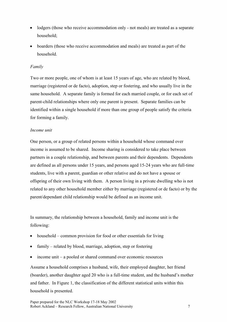
• lodgers (those who receive accommodation only - not meals) are treated as a separate

household;

• boarders (those who receive accommodation and meals) are treated as part of the

household.

Family

Two or more people, one of whom is at least 15 years of age, who are related by blood,

marriage (registered or de facto), adoption, step or fostering, and who usually live in the

same household. A separate family is formed for each married couple, or for each set of

parent-child relationships where only one parent is present. Separate families can be

identified within a single household if more than one group of people satisfy the criteria

for forming a family.

Income unit

One person, or a group of related persons within a household whose command over

income is assumed to be shared. Income sharing is considered to take place between

partners in a couple relationship, and between parents and their dependents. Dependents

are defined as all persons under 15 years, and persons aged 15-24 years who are full-time

students, live with a parent, guardian or other relative and do not have a spouse or

offspring of their own living with them. A person living in a private dwelling who is not

related to any other household member either by marriage (registered or de facto) or by the

parent/dependant child relationship would be defined as an income unit.

In summary, the relationship between a household, family and income unit is the

following:

• household – common provision for food or other essentials for living

• family – related by blood, marriage, adoption, step or fostering

• income unit – a pooled or shared command over economic resources

Assume a household comprises a husband, wife, their employed daughter, her friend

(boarder), another daughter aged 20 who is a full-time student, and the husband’s mother

and father. In Figure 1, the classification of the different statistical units within this

household is presented. Paper prepared for the NLC Workshop 17-18 May 2002 Robert Ackland – Research Fellow, Australian National University 7

Figure 1: Example of multiple statistical unit household

Couple familywith children

household memberNon−family

wife, husband,employed daughter,student daughterFamily and

non−familyhousehold

one or more family units

one or morenon−familymembers

plus

Family units

Couple with dependantchildren income unit

wife, husband, student

employed daughter

One−person income unit

One−person income unit

boarderboarder

Income unitsHousehold type

grandmother, grandfather

Couple−only family Couple−only income unit

grandmother, grandfather

Source: ABS (1995)

While the individual is the unit of observation in many areas of economic research (for

example, the relationship between education and earnings), in analyses of economic

welfare or well-being, the focus is generally on groups of people e.g. households or

families. An analysis of economic welfare using groups of people such as households or

families as the unit of observation relies on a key assumption that economic resources are

shared within the unit. In the context of income as the economic resource, this means that

all members of the unit benefit equally from the income. Note, that the above does not

imply that all members of the unit have the same amount of money spent on their needs as

these needs will obviously vary depending on such characteristics as age and gender

[reference to equivalence scale research].

However, the problem with using households or families as the unit of analysis in welfare

research is that the degree of sharing of economic resources within these groups is highly

variable. Consequently, the ABS make a further assumption that the closer the

relationship between members of households or families, the more like that income will be


shared. The ABS therefore currently recommends that where income is being used as the

measure of economic welfare, the appropriate unit of observation is the income unit.

In certain research contexts, it may be more appropriate to use the household concept. For

example, Smith and Daly (1996) argue that household income is a more reliable indicator

of Indigenous income and status than family income since the concept of household is able

to capture extended kin formations that are reflected in multi-family Indigenous

households.2

For research using the NLC, the income unit approach is probably acceptable. In fact, the

design of the NLC questionnaire ensures that the only possible unit of observation in an

analysis of economic welfare is the income unit. In particular, income information is only

collected for the respondent and his or partner. Therefore with the NLC, we are not able

to construct a complete measure of the economic resources available to households or

families unless these units also comprise a single income unit.

A related point is that while there may be more than one income units within a household

or family, we are only able to measure the economic resources of the income unit of which

the respondent is a member – more here.

Note that while the income unit is the preferred unit of observation for analysis of

economic well-being using the NLC data, we are not able to identify all income units

within the NLC sample. This is because the NLC does not collect information on whether

children are currently in school. Thus in families where there are children aged 15-24

years, we cannot identify whether these children are dependants.

2.3 What income? Private, gross, disposable and final income

Having determined whose income we will be using as an indicator of economic welfare

measuring in the analysis of the NLC data, the next step is to decide on exactly what

income measure will be calculated. As shown in Figure 2, there are four main income

concepts defined by the ABS.3

Private income includes wages and salaries, profits and losses from unincorporated

businesses, income from superannuation and annuities, investment income (including

2 Hunter, Kennedy and Smith (2001) endorse this judgement and present poverty statistics for Indigenous households, as well as statistics based on income units.

3 The discussion in this sub-section is based on ABS (2001).


dividends and rent), and other non-government income. Government direct benefits such

as pensions and unemployment benefits are added to private income to give gross income.

Personal direct taxes (i.e. direct taxes) are deducted from gross income to give disposable

income. Final income is disposable income plus the value of government indirect benefits

for education, health, housing and social security and welfare minus indirect taxes such as

sales tax and GST on selected commodities.

Figure 2: ABS income concepts and components

Private income: from sources other than government benefits

Income from wages, salariesand ownunincorporatedbusiness

Income fromsuperannuationand annuities

Investmentincomeincludingdividends

Gross income: private income plus government direct benefits

Direct tax

Commonwealth,State and localgovernmentcash benefits

Governmentnon−cashbenefits

Indirect tax

Government expenses

Othernon−governmentincome

Disposable income: gross income minus direct tax

Final income: disposable income plus indirect benefits minus indirect taxes

Governmentrevenue

Source: ABS (2001)

Income concepts

plus plus

plus

plus

minus

plus

Income components

minus


In the present paper, the income aggregate used as a measure of economic welfare is gross

income (plus imputed rent, as discussed below). While it should be possible to calculate

disposable income using the NLC data, this would involve imputing the tax rebates that

are available to individuals with different characteristics. ABS (2001) sketches a method

for imputing direct taxes which involves calculating tax rebates according to household

characteristics and tax eligibility for dependent spouses, sole parents, dependent parents,

residential zones, pensioners, beneficiaries, and franked dividend imputation credits. The

imputation of direct taxes using the NLC data was considered to be outside the scope of

the present paper.

Even if a disposable income measure were constructed using the NLC data, it would not

be possible to take the next step and construct final income. Indirect benefits consist of

goods and services provided free or at subsidised prices by the government. While ABS

(2001) presents a method for attributing indirect benefits to households of differing

characteristics, the absence of key information within the NLC would prevent this method

being applied to NLC data. In particular, in order to allocate government indirect benefits

relating to the primary and secondary education and student transportation it is necessary

to know whether children of school age living in the household are currently attending

school. As mentioned above, this information is not available in the NLC data.

With regards to indirect taxes, these cannot be imputed with the NLC data since the

imputation requires information on the expenditure patterns of the different income units.

2.4 Imputed rent as income

The indicator of economic well-being proposed for poverty and welfare analysis using the

NLC data is gross income plus imputed income from owner-occupied housing. The

appropriateness of including imputed rent in an income-based measure of economic well-

being can be illustrated using an example. Consider two identical families, with identical

income, living in identical houses. The difference between the two families is that one

owns the house, while the other is a renter. Since the owner-occupier family does not

have to pay rent, a more accurate measure of the economic resources available to that

family is found by adding to its income the amount of money that it would have to spend

if it were renting the house.

In 1977, the United Nations recommended that imputed rent be included in measures of

total household income used in distributional analysis (UN, 1977), and Yates (1994)

provided the first Australian attempt to implement the UN recommendation using the

1988/89 Household Expenditure Survey (HES). In Yates (1994) there is a discussion of

two methods for calculating imputed rent using survey data. The market rent approach

involves subtracting from an estimate of market rent (calculated by applying a gross rental

rate of return to individual estimates of dwelling value provided in the HES data) the

various costs of home ownership including mortgage interest, depreciation, maintenance

costs and property taxes. It is not possible to use the market rent approach to calculate


imputed rent with the NLC data since the NLC does not record information on housing

costs.

The second method for imputing rent is the opportunity cost approach in which a rate of

return is applied to estimated home equity to obtain an estimate of the income which

would have been received if this equity was held in an interest bearing account. This is

the approach for calculating imputed income from owner-occupied housing that is

employed in the present paper (a five percent rate of return is assumed – this is what Yates

used).

2.5 Summary of income components for NLC data

Details of the construction of the income components for Waves 1 and 2 of the NLC data

are provided in the Annexes. In summary, total “family” income (faminc) is constructed

as the sum of the following income components (see Table 1 for description of income

components): wage, businc, govben, othery, chmain1, chmain2, imprent,

inc_part.

Table 1: Summary of NLC income components Income component Description

wage wage/salary income – of respondent

businc self-employment/business income – of respondent

govben government benefits – received by respondent

othery other income (e.g. rents, dividends, interest) – of respondent

chmain1 child maintenance – paid to respondent

chmain2 child maintenance – paid to partner

chmain child maintenance – total

imprent imputed rent – for house owned by respondent and/or partner

inc_part income of partner

inc_resp sum of wage businc govben othery chmain1 chmain2

3 Preliminary analysis of the NLC income data

In this section, preliminary analysis of the NLC income data is presented. A description of

the construction of the variables referred to in this section is presented in the Annexes.

Most of the results reported here are in the form of Stata output.


3.1 Analysis of Wave 1 income data

3.1.1 Analysis of missing income components

First, it is important to see the extent to which we have missing data for income

components. The following counts are conducted over the full set of 2231 observations.

. count if wage==.; 81 . count if businc==.; 92 . count if govben==.; 142 . count if othery==.; 94 . count if chmain1==.; 62 . count if chmain2==.; 63 . count if imprent==.; 82 . count if inc_resp==.; 27 . count if inc_part==.; 86 . count if completey==1; 1977 . count if noincome==1; 27

3.1.2 Restricting the sample – complete income estimate and ABS income units

The sample of 2231 observations was first restricted to cases where a complete measure of

family income is available (completey=1) – this left a sample of 1977 observations. It

is problematic to lose approximately 11 percent of observations because of incomplete

income information. Further work needs to be done to see if some of these observations

can be “recovered” (this process has already been started).

Second, the sample was restricted to observations where household type corresponds to an

ABS income unit. As mentioned above, it is not possible to identify all income units

within the NLC data (because we do not have information on whether or not children are

currently studying and we do not know if a child of a respondent has offspring living with

him/her). A subset of income units can be identified using: (hhtype2==1 |


hhtype2==2 | hhtype2==3 | hhtype2==5) – in the analysis we are therefore

excluding families where there are adult (15-24 years) children present since we cannot

determine whether these children are dependants as defined by the ABS . The restricted

sample consists of 1202 income units.

3.1.3 Income and per capita income

The following are the descriptive statistics for faminc for the restricted sample:

. sum faminc, det; total family income ------------------------------------------------------------- Percentiles Smallest 1% 8738 323 5% 16739 400 10% 22470 3550 Obs 1202 25% 34398 5486 Sum of Wgt. 1202 50% 53751.5 Mean 64216.68 Largest Std. Dev. 53427.11 75% 78235.4 380000 90% 112728 491120 Variance 2.85e+09 95% 139468 728667 Skewness 5.432587 99% 239854 790160 Kurtosis 57.9492

Per capita income was calculated as pcinc=faminc/hhsize2. The descriptive

statistics for pcinc are:

. sum pcinc, det; pcinc ------------------------------------------------------------- Percentiles Smallest 1% 3937 323 5% 6345.6 400 10% 7831.25 2084.286 Obs 1202 25% 12292.75 2184.5 Sum of Wgt. 1202 50% 21000 Mean 28395.51 Largest Std. Dev. 28417.86 75% 35982.5 192750 90% 54577 350000 Variance 8.08e+08 95% 70405.5 364333.5 Skewness 5.557901 99% 126666.7 395080 Kurtosis 58.05429

3.1.4 Income components

The following are descriptive statistics for the 1202 observations in the restricted sample.

Note that there are 15 income units for which we do not have information on income

components (except imputed rent), because the respondent refused to answer the income

questions. However, the respondent provided an estimate of overall income (excluding

imputed rent), recorded in q249.


Variable | Obs Mean Std. Dev. Min Max -------------+----------------------------------------------------- wage | 1187 30015.33 43082.3 0 780000 businc | 1187 3282.284 14240.51 0 220000 govben | 1187 2183.058 4049.924 0 22308 othery | 1187 1549.8 7232.424 0 150000 chmain | 1202 168.3295 1004.193 0 19240 imprent | 1200 5026.565 7067.669 0 100000 inc_resp | 1202 37222.73 44797.39 0 784160 inc_ref | 15 38947.6 26602.79 9344 118833 inc_part | 1202 21975.75 25216.14 0 111090

The following are descriptive statistics for the income components, calculated only over

those observations where a positive value was recorded.

Variable | Obs Mean Std. Dev. Min Max -------------+----------------------------------------------------- wage | 960 37112.71 45074.95 1 780000 businc | 177 22011.7 30853.43 1 220000 govben | 513 5051.248 4845.326 78 22308 othery | 283 6500.399 13700.19 1 150000 chmain | 52 3891 2996.33 520 19240 imprent | 833 7241.151 7478.677 100 100000 inc_resp | 1185 37756.73 44893.66 120 784160 inc_ref | 15 38947.6 26602.79 9344 118833 inc_part | 779 33908.67 24008.73 1680 111090

3.1.5 Income shares

The following are income shares for the restricted sample:

Variable | Obs Mean Std. Dev. Min Max -------------+----------------------------------------------------- wage_shr | 1187 45.54486 34.26512 0 100 businc_shr | 1187 3.940557 13.42894 0 100 govben_shr | 1187 8.51799 20.25988 0 100 othery_shr | 1187 1.949196 7.371241 0 95.47739 chmain_shr | 1202 .5737121 4.187056 0 100 imprent_shr | 1200 8.097258 11.03624 0 100 inc_part_shr | 1202 31.32586 30.0339 0 100

3.1.6 Per capita income quintiles

A per capita income quintile variable quin was constructed. The quintiles were

constructed over individuals, rather than income units.

. tab quin;

quin | Freq. Percent Cum. ------------+----------------------------------- 1 | 172 14.31 14.31 2 | 190 15.81 30.12 3 | 202 16.81 46.92 4 | 263 21.88 68.80 5 | 375 31.20 100.00 ------------+----------------------------------- Total | 1202 100.00

. tab quin [w=hhsize2];


(frequency weights assumed)


The above shows that there are approximately 14 percent of income units in the bottom

quintile (because poorer households tend to be larger, especially when per capita income is

used as the welfare measure) while 31 percent of households are in the top quintile.

3.1.7 Income shares by quintile

The following shows income shares by quintile groups. As expected, self-

employment/business income is more important for richer income units, and child

maintenance and government benefits are more important for poorer income units.

. table quin, c(mean wage_shr mean businc_shr mean govben_shr mean othery_shr)

format(%9.1f) col row;

-------------------------------------------------------------------------- quin | mean(wage_shr) mean(businc~r) mean(govben~r) mean(othery~r) ----------+--------------------------------------------------------------- 1 | 22.6 2.3 35.2 0.5 2 | 35.2 3.2 14.7 1.0 3 | 40.5 4.1 4.2 1.6 4 | 53.8 2.4 1.4 2.9 5 | 58.4 6.0 0.4 2.6 | Total | 45.5 3.9 8.5 1.9 --------------------------------------------------------------------------

. table quin, c(mean chmain_shr mean imprent_shr mean inc_part_shr)


---------------------------------------------------------- quin | mean(chmain~r) mean(impren~r) mean(inc_pa~r) ----------+----------------------------------------------- 1 | 2.1 8.5 28.5 2 | 1.0 8.4 36.8 3 | 0.4 9.6 39.6 4 | 0.2 7.5 31.7 5 | 0.0 7.4 25.1 | Total | 0.6 8.1 31.3 ----------------------------------------------------------


3.2 Analysis of Wave 2 income data

3.2.1 Analysis of missing income components

As with Wave 1, it is important to see the extent to which we have missing data for

income components.

. count if wage==.; 126 . count if businc==.; 97 . count if govben==.; 65 . count if othery==.; 87 . count if chmain1==.; 11 . count if chmain2==.; 12 . count if imprent==.; 73 . count if inc_resp==.; 0 . count if inc_part==.; 126 . count if completey==1; 1448

3.2.2 Restricting the sample – complete income estimate and ABS income units

The sample of 1768 observations was first restricted to cases where a complete measure of

family income is available (completey=1) – this left a sample of 1448 observations.

Nearly 18 percent of respondents did not provide complete income information – this is

higher than the “incomplete income information” rate found in the Wave 1 data. Further

work will need to be done to see if some of these observations can be recovered.

Second, the sample was restricted to observations where household type corresponds to an

ABS income unit. As with Wave 1, it was not possible to identify all income units in the

Wave 2 data (because there is no information on whether or not children are currently

studying). A subset of income units was identified using: (hhtype2==1 | hhtype2==2

| hhtype2==3 | hhtype2==5). The restricted sample consists of 858 income units.


3.2.3 Income and per capita income

The following are the descriptive statistics for faminc for the restricted sample:

. sum faminc, det;

total family income ------------------------------------------------------------- Percentiles Smallest 1% 10140 0 5% 21668 2840 10% 28100 7020 Obs 858 25% 46108 8320 Sum of Wgt. 858 50% 68665 Mean 85921.39 Largest Std. Dev. 116370.4 75% 98036 740000 90% 143500 863690 Variance 1.35e+10 95% 189027 1252562 Skewness 14.56322 99% 333664 2660154 Kurtosis 295.4922

Mean total income increased by 34 percent between Waves 1 and 2 – this is looked at

further below.

Per capita income was calculated as pcinc=faminc/hhsize2. The descriptive

statistics for pcinc are:

. sum pcinc, det;

pcinc ------------------------------------------------------------- Percentiles Smallest 1% 4680 0 5% 8320 710 10% 10788.57 2291.2 Obs 858 25% 16474.25 3336 Sum of Wgt. 858 50% 27187.5 Mean 38246.37 Largest Std. Dev. 55072.81 75% 43659.8 431750 90% 69584 626281 Variance 3.03e+09 95% 90100 740000 Skewness 9.265088 99% 185823.5 886718 Kurtosis 118.2568

3.2.4 Income components

The following are descriptive statistics for the 858 observations in the restricted sample.

Variable | Obs Mean Std. Dev. Min Max -------------+----------------------------------------------------- wage | 858 36599.07 63081.89 0 1248000 businc | 858 11688.38 73800.57 0 2000000 govben | 858 1880.121 3919.504 0 25662 othery | 858 1703.934 5614.35 0 65000 chmain | 858 147.2121 1079.784 0 16224 imprent | 858 7397.686 20634.07 0 450000 inc_resp | 858 52018.72 109591.7 0 2624000


inc_part | 858 26504.98 29641.56 0 117899

The first thing to note is the large increase in mean business income between Waves 1 and

2 (256 percent), relative to the other income components, as shown in Table 2.

Table 2: Change in mean income component between Waves 1 and 2 Income component Percentage increase/decrease

wage 22

businc 256

govben -14

othery 10

chmain -13

imprent 47

inc_resp 40

inc_part 21

There are two potential reasons why this may have occurred. First, it could be because the

attrition rate for respondents running a business was much lower than the average attrition

rate. Business owners are likely to be less mobile than the average person, and thus easier

to keep track of between waves. It is shown below that the attrition rate for business

owners was indeed lower than for the sample as a whole. However, it is unlikely that

differences in attrition rates accounted for the whole increase in mean business income.

The following are descriptive statistics for the income components, calculated only over

those observations where a positive value was recorded.

Variable | Obs Mean Std. Dev. Min Max -------------+----------------------------------------------------- wage | 718 43735.38 66661.65 1 1248000 businc | 181 55406.81 153283.2 1 2000000 govben | 325 4963.52 5028.224 26 25662 othery | 296 4939.105 8691.258 6 65000 chmain | 25 5052.32 3977.283 104 16224 imprent | 613 10354.35 23781.2 99.9 450000 inc_resp | 850 52508.31 109989.9 26 2624000 inc_part | 550 41347.77 27508.4 1744 117899

In Table 3 it is shown that even when we only look at observations where a positive value

of business income was recorded, the increase in mean business income between the two

waves is still 152 percent. This suggests that the most likely reason for the large increase

in mean business income between the two waves is the change in the structure of the

questionnaire.


Table 3: Change in mean income component between Waves 1 and 2 (conditional) Income component Percentage increase/decrease

wage 18

businc 152

govben -2

othery -24

chmain 30

imprent 43

inc_resp 39

inc_part 22

Note: Percentage changes of average levels of income components, where averages are calculated only over positive

observations.

There was also a large increase in mean imputed rent income between Waves 1 and 2.

Since the structure of the questions relating to housing did not change significantly

between the two waves, it is unlikely that this is an artefact of questionnaire design. As

above, the marked increase mean imputed rent income could be because of a change in the

composition of the sample between the two waves. In particular, since home owners tend

to be less mobile, it is likely that this group were more easily tracked between the waves,

and thus included in Wave 2. Once again, this hypothesis is supported by the data

(attrition rates are presented below). Another reason for the increase in mean imputed rent

between the two surveys is the fact that property prices increased significantly over this

period (recall that imputed rent is calculated using the net value of the property in

question).

3.2.5 Income shares

The following are income shares for the restricted Wave 2 sample:

. sum *_shr;

Variable | Obs Mean Std. Dev. Min Max -------------+----------------------------------------------------- wage_shr | 857 45.21241 32.10232 0 100 businc_shr | 857 8.21314 19.35088 0 100 govben_shr | 857 6.238779 16.73377 0 100 othery_shr | 857 1.775988 5.06969 0 50.50505 chmain_shr | 857 .3703276 2.924468 0 44.38326 imprent_shr | 857 8.153995 10.24133 0 81.38021 inc_part_shr | 857 30.03536 28.64873 0 98.70238


Above, it was found that mean business income increased markedly between Waves 1 and

2 – this is reflected in the income shares where the average share of total income

accounted for by income from business doubled from 4 to 8 percent.

3.2.6 Per capita income quintiles

A per capita income quintile variable quin was constructed. The quintiles were

constructed over individuals, rather than income units.

. tab quin;


. tab quin [w=hhsize2];

(frequency weights assumed)


The above shows that there are approximately 14 percent of income units in the bottom

quintile while 30 percent of household are in the top quintile.

3.2.7 Income shares by quintile

The following shows income shares by quintile groups. As expected, income from wages

and self-employment/business is more important for richer income units, and child

maintenance and government benefits are more important for poorer income units.


. table quin, c(mean wage_shr mean businc_shr mean govben_shr mean othery_shr)


-------------------------------------------------------------------------- quin | mean(wage_shr) mean(businc~r) mean(govben~r) mean(othery~r) ----------+--------------------------------------------------------------- 1 | 31.8 3.6 28.2 0.7 2 | 36.3 7.8 7.7 1.4 3 | 47.2 6.8 3.9 1.9 4 | 49.7 7.9 1.1 1.5 5 | 51.4 11.7 0.5 2.6 | Total | 45.2 8.2 6.2 1.8 --------------------------------------------------------------------------

. table quin, c(mean chmain_shr mean imprent_shr mean inc_part_shr)


---------------------------------------------------------- quin | mean(chmain~r) mean(impren~r) mean(inc_pa~r) ----------+----------------------------------------------- 1 | 1.1 8.4 26.1 2 | 1.1 7.7 37.9 3 | 0.2 7.8 32.2 4 | 0.1 8.3 31.4 5 | 0.0 8.3 25.5 | Total | 0.4 8.2 30.0 ----------------------------------------------------------

3.3 The distributional impact of owner-occupation – Wave 1

It is of interest to see the impact that owner-occupation has on the measured well-being of

the income units in the NLC sample. Yates (1994) used 1988/89 HES data to show that

owner-occupation has a significant distributional impact. The following analysis attempts

to update the Yates (1994) analysis, although it is not possible to make a direct

comparison because the NLC survey uses a sampling frame that is very different to that

used in the HES. In particular, the NLC Wave 1 sample is restricted to only contain

respondents under the age of 54 years. Equity in owner-occupied dwelling and housing

tenure is strongly related to the life-cycle, and for this reason a comparison between the

Wave 1 results and those in Yates (1994) would not be valid.

Table 4 shows wealth, tenure and income variables calculated for different per capita

income deciles. Per capita income deciles were calculated over income units, rather than

individuals. Values have been averaged over all income units, not just owner-occupiers.


Table 4: Owner-occupied housing wealth, tenure and imputed rent (Wave 1)

Per capita income decile

1 2 3 4 5 6 7 8 9 10 total

Wealth ($) ($) ($) ($) ($) ($) ($) ($) ($) ($) ($)

value of dwelling

60,600 79,946 108,160 129,342 154,133 127,950 135,450 134,192 179,067 238,281 134,815

amount owing on

dwelling

22,642 28,819 34,397 32,042 42,048 32,237 40,659 28,275 38,844 47,298 34,731

Tenure (%) (%) (%) (%) (%) (%) (%) (%) (%) (%) (%)

outright owners 8.3 15 14.2 30 25 25.6 21.7 25 32.5 35.5 23.3

owner-purchasers 35.8 45.8 51.7 53.3 53.3 45.5 50 44.2 50.8 44.6 47.5

owner-occupiers 44.2 60.8 65.8 83.3 78.3 71.1 71.7 69.2 83.3 80.2 70.8

Income ($p.w.) ($p.w.) ($p.w.) ($p.w.) ($p.w.) ($p.w.) ($p.w.) ($p.w.) ($p.w.) ($p.w.) ($p.w.)

income 463 636 836 1,036 1,122 1,200 1,302 1,367 1,633 2,742 1,235

per capita income 113 175 233 294 365 455 567 698 893 1,660 546

imputed rent 37 49 71 94 108 92 95 102 135 184 97

[Note: Average values calculated over all income units (not just owner-occupiers). [income includes imputed rent – perhaps should use ex ante income here]


The value of the average dwelling (or gross contribution to wealth) is $134,815 (note –

this average is calculated over all income units and those who do not own their house

would record a zero here). The average amount owing on owner-occupied dwellings is

$34, 731. Imputed rent contributes on average $97 per week to the income of the income

units in the restricted NLC sample. Remember that this is a weighted average of an

imputed income of $137/week for the 70.8 percent of the sample who are owner occupiers

(see table below) and zero for the remainder of the sample who do not own their own

homes. Table 5 clearly shows that imputed rental income is not shared evenly between

owner-purchasers and outright owners. The average outright owner (from above, 34

percent of owner occupiers) enjoys almost four times the imputed rent of the average

owner purchaser.

Table 5: Imputed rent by tenure type and decile

Per capita

income

decile

owner-

purchaser

outright

owner

owner-

occupiers

1 29 116 83

2 33 142 81

3 57 157 108

4 69 151 112

5 72 213 136

6 52 208 131

7 64 206 133

8 48 264 147

9 98 211 162

10 114 312 230

total 61 213 137

The distributional impact of imputed rent can be seen Table 6 which shows the decile

share of two income aggregates – one excluding and one including imputed rent (note that


in both columns, income units have been re-ranked using the appropriate per capita

income measure).

Table 6: Income shares by deciles

Per capita

decile

Income

excluding

imputed

rent

Income

including

imputed

rent

1 3.5 3.7

2 5.0 5.1

3 6.5 6.8

4 8.3 8.4

5 9.7 9.1

6 9.8 9.8

7 10.6 10.5

8 10.7 11.1

9 13.4 13.2

10 22.6 22.3

Gini

coefficient

0.42 0.42

It is apparent that income units in the bottom per capita income quintile receive 8.5

percent of income excluding imputed rent, compared with 8.8 percent of the income

measure that includes imputed rent. While this may appear to not be a significant

distributional impact of including imputed rent, as Yates (1994) points out, the impact of

imputed income on the relative share of those in the bottom quintile is quite large when

one considers changes in inequality that occur over time. The inclusion of imputed rent

into the income measure has no impact on the Gini coefficient.

Table 7 shows the extent to which income unit decile rankings change as a result of

including imputed rent into the income measure. Within each decile, the ranking of

between 8 and 37 percent of income units is changed as a result of the inclusion of

imputed rent. As Yates (1994) found, the impact on rankings is greatest for those income


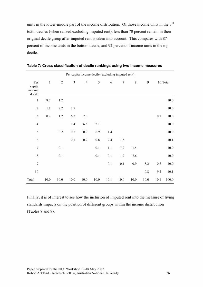
units in the lower-middle part of the income distribution. Of those income units in the 3rd

to5th deciles (when ranked excluding imputed rent), less than 70 percent remain in their

original decile group after imputed rent is taken into account. This compares with 87

percent of income units in the bottom decile, and 92 percent of income units in the top

decile.

Table 7: Cross classification of decile rankings using two income measures

Per capita income decile (excluding imputed rent)

Per capita

income decile

1 2 3 4 5 6 7 8 9 10 Total

1 8.7 1.2 10.0

2 1.1 7.2 1.7 10.0

3 0.2 1.2 6.2 2.3 0.1 10.0

4 1.4 6.5 2.1 10.0

5 0.2 0.5 0.9 6.9 1.4 10.0

6 0.1 0.2 0.8 7.4 1.5 10.1

7 0.1 0.1 1.1 7.2 1.5 10.0

8 0.1 0.1 0.1 1.2 7.6 10.0

9 0.1 0.1 0.9 8.2 0.7 10.0

10 0.8 9.2 10.1

Total 10.0 10.0 10.0 10.0 10.0 10.1 10.0 10.0 10.0 10.1 100.0

Finally, it is of interest to see how the inclusion of imputed rent into the measure of living

standards impacts on the position of different groups within the income distribution

(Tables 8 and 9).


Table 8: Composition of income deciles – income measure excluding imputed rent


1 2 3 4 5 6 7 8 9 10 Total

Tenure

outright owner 15.0 17.5 21.7 26.7 23.3 24.0 19.2 23.3 30.0 32.2 23.3

owner purchaser 40.0 45.8 44.2 50.8 55.8 49.6 52.5 40.8 49.2 46.3 47.5

renter 45.0 36.7 34.2 22.5 20.8 26.4 28.3 35.8 20.8 21.5 29.2

100.0 100.0 100.0 100.0 100.0 100.0 100.0 100.0 100.0 100.0 100.0

Age of

respondent

Under 25 7.5 6.7 6.7 4.2 5.0 5.8 9.2 5.0 3.3 1.7 5.5

25-44 79.2 83.3 80.8 85.8 81.7 74.4 69.2 69.2 69.2 68.6 76.1

45 and over 13.3 10.0 12.5 10.0 13.3 19.8 21.7 25.8 27.5 29.8 18.4

100.0 100.0 100.0 100.0 100.0 100.0 100.0 100.0 100.0 100.0 100.0

Family type

lone 7.5 10.8 9.2 3.3 6.7 20.7 27.5 37.5 37.5 44.6 20.5

couple, no kids 3.3 5.0 6.7 10.8 15.8 26.4 37.5 44.2 47.5 43.0 24.0

sole parent, kids 23.3 19.2 6.7 9.2 6.7 6.6 1.7 1.7 0.0 4.1 7.9

couple, kids 65.8 65.0 77.5 76.7 70.8 46.3 33.3 16.7 15.0 8.3 47.5

100.0 100.0 100.0 100.0 100.0 100.0 100.0 100.0 100.0 100.0 100.0


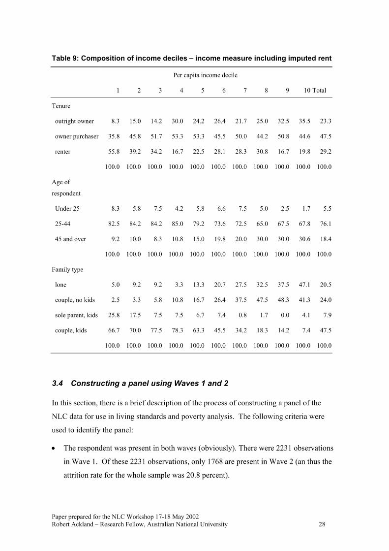
Table 9: Composition of income deciles – income measure including imputed rent


1 2 3 4 5 6 7 8 9 10 Total

Tenure

outright owner 8.3 15.0 14.2 30.0 24.2 26.4 21.7 25.0 32.5 35.5 23.3

owner purchaser 35.8 45.8 51.7 53.3 53.3 45.5 50.0 44.2 50.8 44.6 47.5

renter 55.8 39.2 34.2 16.7 22.5 28.1 28.3 30.8 16.7 19.8 29.2

100.0 100.0 100.0 100.0 100.0 100.0 100.0 100.0 100.0 100.0 100.0

Age of

respondent

Under 25 8.3 5.8 7.5 4.2 5.8 6.6 7.5 5.0 2.5 1.7 5.5

25-44 82.5 84.2 84.2 85.0 79.2 73.6 72.5 65.0 67.5 67.8 76.1

45 and over 9.2 10.0 8.3 10.8 15.0 19.8 20.0 30.0 30.0 30.6 18.4

100.0 100.0 100.0 100.0 100.0 100.0 100.0 100.0 100.0 100.0 100.0

Family type

lone 5.0 9.2 9.2 3.3 13.3 20.7 27.5 32.5 37.5 47.1 20.5

couple, no kids 2.5 3.3 5.8 10.8 16.7 26.4 37.5 47.5 48.3 41.3 24.0

sole parent, kids 25.8 17.5 7.5 7.5 6.7 7.4 0.8 1.7 0.0 4.1 7.9

couple, kids 66.7 70.0 77.5 78.3 63.3 45.5 34.2 18.3 14.2 7.4 47.5

100.0 100.0 100.0 100.0 100.0 100.0 100.0 100.0 100.0 100.0 100.0

3.4 Constructing a panel using Waves 1 and 2

In this section, there is a brief description of the process of constructing a panel of the

NLC data for use in living standards and poverty analysis. The following criteria were

used to identify the panel:

• The respondent was present in both waves (obviously). There were 2231 observations

in Wave 1. Of these 2231 observations, only 1768 are present in Wave 2 (an thus the

attrition rate for the whole sample was 20.8 percent).


• The respondent was a part of an ABS-defined income unit in both waves. This

selection criteria reduces the panel from 1768 observations to 820 observations.

• The respondent provided complete income information in both waves. This selection

criteria reduces the panel from 820 observations to 638 observations.

It is apparent that the above criteria used for identifying a panel are too stringent: too

much information is being lost. On a practical level, most econometric analysis cannot be

adequately conducted using a panel of only 638 observations. As previously discussed,

there needs to be an attempt to “salvage” some of the observations that have been omitted

because of incomplete income information. Relatedly, the criterion for deciding whether

complete income information has been provided may need to be relaxed so that a

respondent who provided the “most important” income information will remain in the

panel. Also, in Wave 3 of the NLC, the questionnaire needs to be modified so that the

schooling status of children can be identified (this will mean more families in the NLC

will be able to be classified as ABS income units and thus included in the analysis).

Table 10 shows the percentage of respondents in Wave 1 who were not present in Wave 2

of the NLC. As discussed above, respondents with business and imputed rent income

have lower attrition rates than average. Respondents who were identified as living in

ABS-defined income units had attrition rates similar to that found with the whole sample.

Table 10: NLC attrition rates

Whole sample Respondents in income unit in

Wave 1

All respondents 20.8 20.9

Respondents with business

income

15.1 15.2

Respondents with imputed rent

income

15.2 16.1

4 Conclusions

In this paper, the process of the construction of an income-based measure of well-being for

the NLC data was described. Preliminary analysis of the income data was presented for


both waves, and a more detailed study of the distributional impact of imputed rent was

conducted using the Wave 1 data.

Several issues relating to the NLC data were raised. These include the following:

• The percentage of income units with a complete income response is small. The

percentage of respondents giving incomplete income information in Wave 1 was 11

percent, while in Wave 2 it had increased to 18 percent. The process of salvaging

some of these observations (by trying to reconstruct income information using

responses to other questions) is already underway. In the present paper, only

observations with complete responses to all income questions were included in the

analysis. In future analysis, it may be preferable to keep those observations where

responses were given to the most important income questions (e.g. wages) and be more

lenient to cases where less important income information is missing.

• A major problem with the NLC data is that the absence of a question relating to the

schooling status of children means that it is impossible to identify all ABS income

units within the data. In particular, children aged 15-24 years must be full-time

students for them to be included in an income unit. In the third wave of the NLC it

will be important to include a question on current schooling status of children, and also

retrospective questions so that the schooling status of children at the time of the

previous two waves can be determined.

• There is a question regarding the accuracy of the business/self employment income

data – there was a large increase in this income component between waves. This

needs to be looked at further.

• Depending on the demand by NLC researchers, there may need to be further work on

constructing a disposable income measure.


5 References

Australian Bureau of Statistics (1995), A Provisional Framework for Household Income,

Consumption, Saving and Wealth (1995), Cat. no. 6549.0, ABS, Canberra.

------------------------------------- (2001), Government Benefits, Taxes and Household

Income, Australia, Cat. no. 6537.0, ABS, Canberra.

Hunter, B.H., Kennedy, S. and D. Smith (2001), “Sensitivity of Australian income

distributions to choice of equivalence scale: Exploring some parameters of Indigenous

incomes,” Centre for Aboriginal Economic Policy Research Working Paper No.

11/2001, ANU, Canberra.

Smith, D. and A.E. Daly (1996), “The economic status of Indigenous Australian

households: A statistical and ethnographic analysis,” Centre for Aboriginal Economic

Policy Research Discussion Paper No. 109, ANU, Canberra.

Yates, J. (1994), “Imputed Rent and Income Distribution,” Review of Income and Wealth,

40(1), 43-66.


Annexes

The purpose of the following annexes is to outline the methods used in constructing an

estimate of family income for Waves 1 and 2 of the Negotiating the Life Course (NLC)

survey. This annexes describe the contents of the Stata (version 7) do files that were used

to construct family income (this paper is included in a zip file which contains Stata do

files, raw NLC data files for Wave 1 and 2 and constructed data files). Users of the

constructed data sets are advised to read the annexes so that they are aware of the

decisions made in constructing the income data and any inherent limitations in the

estimates. It is also suggested that users look carefully at the Stata do files.

It should be noted that these Stata do files are provided to NLC researchers so that they

can see exactly how each constructed variable has been created. It is the responsibility of

every researcher who uses these data to check that the variable they are using is what they

want. While every attempt has been made to ensure the accuracy of these Stata do files,

they are essentially provided "as is" and without warranty of any kind. If a researcher

finds an error in the Stata do files, or believes that a variable should be created in a

different way, please contact the author.

Annex 1 Data construction for Wave 1

There are 2231 observations in the Wave 1 data set nlc97.dta. The data were collected

between November 1996 and April 1997.

A1.1 Missing value codes in Wave 1

-3 – pulled out during the survey? Codes: -9, -8, -2, -1

A1.2 Household demography variables

The file hhdemog.do constructs basic household demography variables and outputs

them to the constructed (household-level) data set hhdemog.dta. The following

variables are contained in hhdemog.dta:


Contains data from hhdemog.dta obs: 2,231 vars: 53 4 Apr 2002 21:31 size: 129,398 (97.9% of memory free) ------------------------------------------------------------------------------- storage display value variable name type format label variable label ------------------------------------------------------------------------------- id int %8.0g yearint byte %9.0g year of interview monthint byte %9.0g month of interview ager byte %8.0g age of respondent (from d1015) ager2 byte %9.0g age of respondent ch_n byte %9.0g # children (<15 yrs) at home adch_n byte %9.0g # adult children at home ch1_age byte %9.0g age of child -1- ch2_age byte %9.0g age of child -2- ch3_age byte %9.0g age of child -3- ch4_age byte %9.0g age of child -4- ch5_age byte %9.0g age of child -5- ch6_age byte %9.0g age of child -6- ch7_age byte %9.0g age of child -7- ch8_age byte %9.0g age of child -8- ch9_age byte %9.0g age of child -9- ch10_age byte %9.0g age of child -10- ch11_age byte %9.0g age of child -11- ch1_gen byte %9.0g gender of child -1- ch2_gen byte %9.0g gender of child -2- ch3_gen byte %9.0g gender of child -3- ch4_gen byte %9.0g gender of child -4- ch5_gen byte %9.0g gender of child -5- ch6_gen byte %9.0g gender of child -6- ch7_gen byte %9.0g gender of child -7- ch8_gen byte %9.0g gender of child -8- ch9_gen byte %9.0g gender of child -9- ch10_gen byte %9.0g gender of child -10- ch11_gen byte %9.0g gender of child -11- ch1_hom byte %9.0g child -1- at home? ch2_hom byte %9.0g child -2- at home? ch3_hom byte %9.0g child -3- at home? ch4_hom byte %9.0g child -4- at home? ch5_hom byte %9.0g child -5- at home? ch6_hom byte %9.0g child -6- at home? ch7_hom byte %9.0g child -7- at home? ch8_hom byte %9.0g child -8- at home? ch9_hom byte %9.0g child -9- at home? ch10_hom byte %9.0g child -10- at home? ch11_hom byte %9.0g child -11- at home? childmiss byte %9.0g missing info on age child(ren) relat2 byte %22.0g relat relat. of person -2- to resp. relat3 byte %22.0g relat relat. of person -3- to resp. relat4 byte %22.0g relat relat. of person -4- to resp. relat5 byte %22.0g relat relat. of person -5- to resp. relat6 byte %22.0g relat relat. of person -6- to resp. relat7 byte %22.0g relat relat. of person -7- to resp. relat8 byte %22.0g relat relat. of person -8- to resp. relat9 byte %22.0g relat relat. of person -9- to resp. hhsize byte %8.0g q280 household size (from d1015) hhsize2 byte %9.0g household size hhtype byte %8.0g hhtype household type (from d1015) hhtype2 byte %23.0g hhtype2f household type ------------------------------------------------------------------------------- Sorted by: id


• ager2 (age of respondent) created as ager2 = yearint – q26 (year of birth of

respondent).

• Using q25 (month of birth of respondent), an adjustment to ager2 was then made if

the respondent had not yet had birthday in the year of interview (note: it was assumed

that if birthday was in same month as interview, then respondent would have had

birthday).

• ager2 differs from ager (age of respondent variable contained in d1015.dta) by

one year for 715 respondents.

A1.2.2 Demographic information on children (living at home and otherwise)

• Some adjustments were first made to raw data where year of birth, month of birth and

gender of children were missing in Wave 1 but supplied in Wave 2.

• ch*_gen (gender of child), where “*” ranges from 1 to 11 was constructed using

q8a*.

• ch*_age (age of child) was constructed using q9a* and q10a*. As for age of

respondent, an adjustment was made where child had not yet had birthday in year of

interview. Note that month of birth was not supplied for some children – this was

estimated assuming a uniform distribution.

• ch*_hom (dummy variable = 1 if child lives at home) was constructed using q11a*.

• A dummy variable childmiss (=1 if age of child(ren) living at home not supplied)

was created. One household was identified as not providing information on the age of

child(ren) living at home.

A1.2.3 Fixing some inconsistencies in the data on children

There were some inconsistencies between the household roster data and the data on the

presence of children in the household – these were fixed.

A1.2.4 Calculate number of children and adult children living at home

• ch_n is the number of children (under 15 years old) living at home.

• adch_n is the number of children (15 years and older) living at home.


A1.2.5 Find relationship of household members to respondent

relat* (where * ranges from 2 to 9) gives the relationship of household member * to the

respondent and is constructed using q282a*. relat* has the following categories:

2 "partner"

3 "child/step-child"

4 "Father/father-in-law"

5 "Mother/mother-in-law"

6 "Brother/brother-in-law"

7 "Sister/sister-in-law"

8 "Grandfather"

9 "Grandmother"

10 "Other male rel."

11 "Other female rel."

12 "Other male"

13 "Other female"

There were no cases of missing household roster information (therefore the variable

rostermiss, which appears in Wave 2, is not present in Wave 1).

A1.2.6 Inconsistencies in the data comparison between q20 and roster are noted

Several inconsistencies between the information in q20 (partnership status of respondent)

and the household roster variables (q282a*) were noted but have not been fixed at this

stage.

A1.2.7 Household size

Household size (hhsize2) was calculated using the relat* variables. hhsize2 is

identical to hhsize (household size constructed variable contained in d1015.dta).

Note: there has been no check of the consistency between hhsize2, ch_n and adch_n.

A1.2.8 Household type/composition

Household type (hhtype2) was created using relat*, ch_n and adch_n. It has the

following categories:

1 "lone"


2 "couple, no kids"

3 "sole parent, kids"

4 "sole parent, adult kids"

5 "couple, kids"

6 "couple, adkids"

7 "other"

There are several instances of inconsistencies between hhtype2 and hhtype

(household type constructed variable contained in d1015.dta).

A1.3 Family income variables

The file income.do constructs family income variables and outputs them to the

constructed (household-level) data set income.dta. The overall aim of the code in

income.do is to construct an estimate of gross (before tax) family income for the

1995/96 financial year.

The following variables are contained in income.dta: Contains data from income.dta obs: 2,231 vars: 15 5 Apr 2002 00:37 size: 107,088 (99.0% of memory free) ------------------------------------------------------------------------------- storage display value variable name type format label variable label ------------------------------------------------------------------------------- id int %8.0g wage float %9.0g wages businc float %9.0g self-employment/business income govben int %9.0g government benefits othery float %9.0g other income chmain int %9.0g child maintenance - total chmain1 int %9.0g child maintenance - respondent chmain2 int %9.0g child maintenance - partner imprent float %9.0g imputed rent inc_resp float %9.0g total income - respondent havepart byte %9.0g dummy - living with partner inc_part float %9.0g income of partner inc_ref float %9.0g income (from q249) faminc float %9.0g total family income completey byte %9.0g dummy - complete est. of faminc noincome byte %9.0g dummy - no income information ------------------------------------------------------------------------------- Sorted by: id


Variable | Obs Mean Std. Dev. Min Max -------------+----------------------------------------------------- id | 2231 1306.146 738.2013 1 2574 wage | 2150 27025.33 40332.22 0 832000 businc | 2139 3373.117 15915.87 0 250000 govben | 2089 2078.693 3886.414 0 22308 othery | 2137 1371.699 7049.351 0 150000 chmain | 2204 169.9201 1104.113 0 21580 chmain1 | 2169 156.7192 1079.834 0 21580 chmain2 | 2168 15.95018 262.973 0 7800 imprent | 2149 4840.716 8789.333 0 250000 inc_resp | 2204 33628.48 42492.83 0 832000 havepart | 2204 .6302178 .4828552 0 1 inc_part | 2145 19261.05 24973.71 0 111090 inc_ref | 33 34829.67 23843.74 0 118833 faminc | 2204 57093.83 52748.24 0 835750 completey | 2231 .8861497 .3177006 0 1 noincome | 2231 .0121022 .1093668 0 1

A1.3.1 People who refused to give detailed income information

Sixty people refused to answer q236 (wages) – these people were skipped to q249

(estimated grouped income) and 33 of the 60 gave a response to this question. It is

impossible to give an income estimate for the 27 people who refused to answer both q236

and q249 and it is recommended that these people be dropped from analysis that involves

the use of family income. The dummy variable noincome (=1 if respondent refused to

answer both q236 and q249) identifies these 27 people.

For the 33 people who answered q249, it was necessary to convert from an income group

(e.g. $15,600 - $20,799) to an income amount within the range. The conversion from

income group to a quasi-continuous measure was done by fitting a log-normal distribution

to the grouped data (see explanatory note by T. Breusch). The quasi-continuous income

value (based on q249) is called inc_ref, and it is only defined for the 33 individuals

who refused q236 but answered q249.

A1.3.2 Wages

The construction of an annual wage variable (wage) involved q236 (wage/salary earned),

q237 (frequency of receipt of income), q238 (income - gross [before tax] or net [after

tax])..

The following decisions were made:

• q236=9 and q236=99, while unusual values, were treated as legitimate (30 cases)

• if q236=-8, then wage=0 (4 cases). Note that in general, the missing value code –8

was treated exactly the same as missing value codes –2, –1 when we have reason


(based on other questions) to expect that there should have been a legitimate value

given for an income component. Only with wages was –8 treated differently to –2, -1

(because we are not able to construct a dummy variable indicating whether or not

wages were received).

• if q236=-1, then wage=. (20 cases)

• if q237=-3 (this is not a valid missing code for Wave 1), then wage=. (1 case)

One problem encountered was the fact that while the majority of individuals reported

gross wages, 393 reported net wages. It was decided to convert net wages to gross wages

– this was done using the tax scales that applied in 1995/96. Implicit in the conversion of

net to gross wages is the assumption that [XX – get argument from Trevor again]

A1.3.3 Self-employment/business income

The construction of the annual self-employment/business income variable (businc)

involved: q239 (did you receive income from self-employment or business?) and q240

(amount of business income, before tax but after expenses).

• A variable indicating receipt of business income (businc_r) was created with

businc_r=1 if q239=1 (“yes”), businc_r=0 if q239=2 (“no”), businc_r=. if

q239=-1|q239=-2.

• if businc_r=0 then businc=0 (note: all these people skipped q240, as expected)

• if businc_r=. then businc=. (4 cases – all skipped q240)

• if businc_r=1 then businc=q240

• if businc_r=1&(q240=-1|q240=-2|q240=-8) then businc=. (28 cases)

• q240=99, while an unusual value, was treated as legitimate (2 cases)

A1.3.4 Government benefits

The construction of annual government benefits income (govben) involved: q241_* (21

variables indicating receipt of particular types of benefits), q242_* (4 variables checking

whether family or child benefits received), q243 (total amount of benefits received per

fortnight).


• A person was considered to be in receipt of some type of benefit if answered: “yes” to

q241_1 (are you receiving any government pensions, benefits or allowances) OR

“yes” to any of q241_2-q241_21 (receipt of particular types of benefits) OR “yes”

to q242_1 (checking question about receipt of child or family payments) OR “yes” to

any of q242_2-q242_4 (checking question about receipt of particular types of child

or family payments)

• There were some coding inconsistencies. Two people said yes to q241_1, but no to

all payment categories (q241_2-q241_21) – both of these people answered q243=-

9, so it was decided to classify them as not being in receipt of government benefit.

Five people (including 3 new people i.e. different to the two identified above) said yes

to q242_1, but no to all family and child payment categories (q242_2-q242_4) –

of the 3 new people, 2 answered q243=-9 and they were classified as not being in

receipt of government benefit. However, one person answered q243=60 – it was

decided to classify this person as being in receipt of government benefit.

• If a person was considered to not be in receipt of some type of benefit, then

govben=0

• if a person was considered to be in receipt of some type of benefit, but (q243=-

1|q243=-2|q243=-8) then govben=. (78 cases)

• q243=99, while an unusual value, was treated as legitimate (1 case)

• A value of q243=999 was considered suspicious and set to missing (2 cases)

A1.3.5 Other income

The construction of annual other income earned (othery) involved q244 (variable

indicating whether other income such as rents, dividends or interest earned) and q245

(amount of other income earned).

A variable indicating receipt of other income (othery_r) was created with

othery_r=1 if q244=1 (“yes”), othery_r=0 if q244=2 (“no”), othery_r=. if

q244=-1|q244=-2

if othery_r=0 then othery=0

if othery_r=. then othery=. (3 cases – all skipped q245)


if othery_r=1 then othery=q245

q245=99, while an unusual value, was treated as legitimate (2 cases)

if a person was considered to be in receipt of other income, but (q245=-1|q245=-

2|q245=-8) then othery=. (31 cases)

A1.3.6 Child maintenance – received by respondent

The construction of child maintenance income paid to respondent (chmain1) involved

q246 (variable indicating whether child maintenance received by respondent, partner or

both) and q247 (amount received by respondent per week).

A variable indicating whether respondent receives child maintenance (chmain1r)

was created with chmain1r=1 if q246=1 (“yes, I do”) or q246=3 (“yes, we both

do”), chmain1r =0 if q246=4 (“no”), chmain1r =. if q246=-3

if chmain1r=0 then chmain1=0

if chmain1r=. then chmain1=. (2 cases – both skipped q247)

if chmain1r=1 then chmain=q247*52

A1.3.7 Child maintenance – received by partner

The construction of child maintenance income paid to partner (chmain2) involved q246

(variable indicating whether child maintenance received by respondent, partner or both)

and q248 (amount received by partner per week).

A variable indicating whether partner receives child maintenance (chmain2r) was

created with chmain2r=1 if q246=2 (“yes, my partner does”) or q246=3 (“yes, we

both do”), chmain2r =0 if q246=4 (“no”), chmain2r =. if q246=-3


if chmain2r=. then chmain2=. (2 cases – both skipped q248)

if chmain2r=1 then chmain2=q248*52

if chmain2r=1 but q248=-1, then chmain2=. (1 case)


A1.3.8 Partner’s income

Parner’s annual income (inc_part) was created using q250 (partner’s annual income

in income groups) and q20 (partner status).

A variable indicating whether the respondent is living with a partner was created with

havepart=1 if q20==3 (not married but living with partner) | q20==4 (living with

husband/wife)

inc_part=0 if havepart=0. Note – one person for whom havepart=0, gave

q250=7 and one person gave q250=-2

inc_part=. if havepart==1&(inc_part==-1|inc_part==-2|inc_part==-

9) – 59 cases

for those respondents with havepart=1 and a legitimate response to q250,

inc_part was found using the estimation approach outlined above (where grouped

data converted to quasi-continuous variable using method proposed by T. Breusch)

A1.3.9 Imputed rent

Annual imputed rent (imprent) was calculated using q252 (whether own house), q253

(whether fully own house), q255 (amount owing on house), q256 (estimated market

value of house).

A dummy variable indicating ownership of home was created with ownhouse=1 if

q252=1

A dummy variable indicating full ownership of home was created with ownfull=1 if

q253=1

The amount owing on home (owing) is equal to q255. Note that owing=0 if

ownfull=1. Note that owing=. when ownhouse!=1. Note that owing=. for 35

cases with ownhouse=1 but did not give a legitimate answer to q255

The market value of the house (value) is equal to q256. Note that value=. if

ownhouse!=1. Note that value=. for 27 cases with ownhouse=1 but did not give

a legitimate answer to q256


Equity in the home was calculated with equity=value-owing. Note that for 55

cases with ownhouse=1, equity=. because either value or owing was missing. For

15 cases with equity<0, equity was set to 0

Imputed rent (imprent) was calculated as imprent=0.05*equity [XX – need to

give rationale for this calculation]

A1.3.10 Respondent’s total income

Respondent’s income (inc_resp) was calcuated as the sum of wage, businc,

govben, othery, chmain1, and chmain2. Note that inc_resp=inc_ref for the

33 people who refused to answer detailed income questions but answered q249.

A1.3.11 Family income

Family income (faminc) was calculated as the sum of inc_resp, inc_part and

imprent.

A1.3.12 Accuracy of income estimate

Note –the Stata command used to calculate family income – rsum() – converts missing

values to zeros. Thus it is possible that a respondent giving missing values for all income

compenents records faminc=0, rather than faminc=.. It is therefore important that

users of the constructed income data identify the households for which there is a legitimate

estimate of family income available.

If there is a missing value for any of the compenents of family income, then we do not

have a complete estimate of family income. The dummy variable completey indicates

whether the estimate of family income is complete with completey=1 if (wage!=. &

businc!=. & govben!=. & othery!=. & chmain1!=. & chmain2!=. &

inc_part!=. & imprent!=.).

A dummy variable noincome with noincome=1 if the respondent refused to give any

income information (this applied to 27 cases).


A1.4 Dataset containing “core” constructed variables

The file core.do merges income.dta and hhdemog.dta and outputs a constructed

(household-level) data set of “core” variables called core.dta. The following variables

are contained in core.dta:

Contains data from C:\statawrk\nlc\wave1\core.dta obs: 2,231 vars: 18 5 Apr 2002 00:45 size: 107,088 (98.9% of memory free) ------------------------------------------------------------------------------- storage display value variable name type format label variable label ------------------------------------------------------------------------------- id int %8.0g ager2 byte %9.0g age of respondent hhtype2 byte %23.0g hhtype2f household type hhsize2 byte %9.0g household size childmiss byte %9.0g missing info on age child(ren) wage float %9.0g wages businc float %9.0g self-employment/business income govben int %9.0g government benefits othery float %9.0g other income chmain int %9.0g child maintenance - total chmain1 int %9.0g child maintenance - respondent chmain2 int %9.0g child maintenance - partner imprent float %9.0g imputed rent inc_resp float %9.0g total income - respondent inc_part float %9.0g income of partner completey byte %9.0g dummy - complete est. of faminc noincome byte %9.0g dummy - no income information faminc float %9.0g total family income ------------------------------------------------------------------------------- Sorted by: id . sum Variable | Obs Mean Std. Dev. Min Max -------------+----------------------------------------------------- id | 2231 1306.146 738.2013 1 2574 ager2 | 2231 36.06768 9.564902 18 55 hhtype2 | 2231 4.542806 2.064831 1 7 hhsize2 | 2231 3.212909 1.4309 1 9 childmiss | 2231 .0004482 .0211714 0 1 wage | 2150 27025.33 40332.22 0 832000 businc | 2139 3373.117 15915.87 0 250000 govben | 2089 2078.693 3886.414 0 22308 othery | 2137 1371.699 7049.351 0 150000 chmain | 2204 169.9201 1104.113 0 21580 chmain1 | 2169 156.7192 1079.834 0 21580 chmain2 | 2168 15.95018 262.973 0 7800 imprent | 2149 4840.716 8789.333 0 250000 inc_resp | 2204 33628.48 42492.83 0 832000 inc_part | 2145 19261.05 24973.71 0 111090 completey | 2231 .8861497 .3177006 0 1 noincome | 2231 .0121022 .1093668 0 1 faminc | 2204 57093.83 52748.24 0 835750


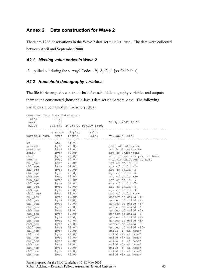
Annex 2 Data construction for Wave 2

There are 1768 observations in the Wave 2 data set nlc00.dta. The data were collected

between April and September 2000.

A2.1 Missing value codes in Wave 2

-3 – pulled out during the survey? Codes: -9, -8, -2, -1 [xx finish this]

A2.2 Household demography variables

The file hhdemog.do constructs basic household demography variables and outputs

them to the constructed (household-level) data set hhdemog.dta. The following

variables are contained in hhdemog.dta:

Contains data from hhdemog.dta obs: 1,768 vars: 53 12 Apr 2002 12:23 size: 102,544 (97.3% of memory free) ------------------------------------------------------------------------------- storage display value variable name type format label variable label ------------------------------------------------------------------------------- id int %8.0g yearint byte %9.0g year of interview monthint byte %9.0g month of interview ager2 byte %9.0g age of respondent ch_n byte %9.0g # children (<15 yrs) at home adch_n byte %9.0g # adult children at home ch1_age byte %9.0g age of child -1- ch2_age byte %9.0g age of child -2- ch3_age byte %9.0g age of child -3- ch4_age byte %9.0g age of child -4- ch5_age byte %9.0g age of child -5- ch6_age byte %9.0g age of child -6- ch7_age byte %9.0g age of child -7- ch8_age byte %9.0g age of child -8- ch9_age byte %9.0g age of child -9- ch10_age byte %9.0g age of child -10- ch1_gen byte %9.0g gender of child -1- ch2_gen byte %9.0g gender of child -2- ch3_gen byte %9.0g gender of child -3- ch4_gen byte %9.0g gender of child -4- ch5_gen byte %9.0g gender of child -5- ch6_gen byte %9.0g gender of child -6- ch7_gen byte %9.0g gender of child -7- ch8_gen byte %9.0g gender of child -8- ch9_gen byte %9.0g gender of child -9- ch10_gen byte %9.0g gender of child -10- ch1_hom byte %9.0g child -1- at home? ch2_hom byte %9.0g child -2- at home? ch3_hom byte %9.0g child -3- at home? ch4_hom byte %9.0g child -4- at home? ch5_hom byte %9.0g child -5- at home? ch6_hom byte %9.0g child -6- at home? ch7_hom byte %9.0g child -7- at home?


ch8_hom byte %9.0g child -8- at home?

ch9_hom byte %9.0g child -9- at home? ch10_hom byte %9.0g child -10- at home? childmiss byte %9.0g missing info on age child(ren) relat2 byte %22.0g relat relat. of person -2- to resp. relat3 byte %22.0g relat relat. of person -3- to resp. relat4 byte %22.0g relat relat. of person -4- to resp. relat5 byte %22.0g relat relat. of person -5- to resp. relat6 byte %22.0g relat relat. of person -6- to resp. relat7 byte %22.0g relat relat. of person -7- to resp. relat8 byte %22.0g relat relat. of person -8- to resp. relat9 byte %22.0g relat relat. of person -9- to resp. relat10 byte %22.0g relat relat. of person -10- to resp. relat11 byte %22.0g relat relat. of person -11- to resp. relat12 byte %22.0g relat relat. of person -12- to resp. relat13 byte %22.0g relat relat. of person -13- to resp. relat14 byte %22.0g relat relat. of person -14- to resp. hhsize byte %8.0g q266 household size (from nlc03jul) hhsize2 byte %9.0g household size hhtype2 byte %13.0g hhtype2f household type rostermiss byte %9.0g dummy - missing roster info ------------------------------------------------------------------------------- Sorted by: id

Variable | Obs Mean Std. Dev. Min Max -------------+----------------------------------------------------- id | 1768 1316.134 735.2395 1 2574 yearint | 1768 100 0 100 100 monthint | 1768 5.424208 .7634268 4 9 ager2 | 1768 39.92477 9.447589 21 59 ch_n | 1768 .8438914 1.115034 0 6 adch_n | 1768 .3535068 .7081298 0 5 ch1_age | 1281 15.94223 9.284552 0 38 ch2_age | 1061 14.52498 8.933749 0 36 ch3_age | 489 13.86912 8.455237 0 34 ch4_age | 181 12.65746 7.901042 0 32 ch5_age | 51 11.82353 7.706376 0 29 ch6_age | 14 8.928571 6.207493 1 20 ch7_age | 6 10.16667 7.782459 3 22 ch8_age | 1 3 . 3 3 ch9_age | 1 14 . 14 14 ch10_age | 0 ch1_gen | 1285 1.522957 .4996671 1 2 ch2_gen | 1067 1.501406 .5002325 1 2 ch3_gen | 492 1.512195 .50036 1 2 ch4_gen | 183 1.497268 .5013643 1 2 ch5_gen | 52 1.519231 .5045046 1 2 ch6_gen | 14 1.571429 .5135526 1 2 ch7_gen | 6 1.333333 .5163978 1 2 ch8_gen | 1 1 . 1 1 ch9_gen | 1 2 . 2 2 ch10_gen | 0 ch1_hom | 1292 .6571207 .4748553 0 1 ch2_hom | 1074 .6880819 .4634924 0 1 ch3_hom | 501 .6986028 .4593235 0 1 ch4_hom | 192 .65625 .4762006 0 1 ch5_hom | 60 .6833333 .4691018 0 1 ch6_hom | 22 .5909091 .5032363 0 1 ch7_hom | 14 .2857143 .4688072 0 1 ch8_hom | 9 0 0 0 0 ch9_hom | 8 0 0 0 0 ch10_hom | 7 0 0 0 0 childmiss | 1768 .0011312 .0336241 0 1 relat2 | 1558 3.105905 3.289454 2 17 relat3 | 1137 4.595427 4.052896 2 17 relat4 | 790 4.458228 3.83039 2 17 relat5 | 318 4.63522 3.995141 2 17 relat6 | 99 4.939394 4.323213 3 17 relat7 | 20 6.4 5.413434 2 17


relat8 | 7 6.428571 5.883795 3 16

relat9 | 2 9.5 9.192388 3 16 relat10 | 1 16 . 16 16 relat11 | 1 16 . 16 16 relat12 | 1 16 . 16 16 relat13 | 1 16 . 16 16 relat14 | 1 17 . 17 17 hhsize | 1750 3.249143 1.440525 1 14 hhsize2 | 1750 3.249143 1.440525 1 14 hhtype2 | 1750 4.529143 2.052486 1 7 rostermiss | 1768 .010181 .1004144 0 1

The structure of hhdemog.do is as follows.

A2.2.1 Age of respondent

• yearint (year of interview) was set to 100 (all interviews were conducted in 2000)

and monthint (month of interview) was constructed from the string variable e_.

• ager2 (age of respondent) created as ager2 = yearint – q1y (year of birth of

respondent).

• Using q1m (month of birth of respondent), an adjustment to ager2 was then made if

the respondent had not yet had birthday in the year of interview (note: it was assumed

that if birthday was in same month as interview, then respondent would have had

birthday).

A2.2.2 Demographic information on children (living at home and otherwise)

• Some adjustments were first made to raw data where year of birth, month of birth and

gender of children were missing in Wave 2 but supplied in Wave 1 (or, in the case of

month of birth estimated using a uniform distribution, as described above).

• ch*_gen (gender of child), where “*” ranges from 1 to 10 was constructed using

q146a*.

• ch*_age (age of child) was constructed using q147a* and q148a*. As for age of

respondent, an adjustment was made where child had not yet had birthday in year of

interview. Note that month of birth was not supplied for some children (and could not

be found using Wave 1 data) – this was estimated assuming a uniform distribution.

• ch*_hom (dummy variable = 1 if child lives at home) was constructed using

q149a*.


• A dummy variable childmiss (=1 if age of child(ren) living at home not supplied)

was created. Two households were identified as not providing information on the age

of child(ren) living at home.

A2.2.3 Fixing some inconsistencies in the data on children

At this stage, no inconsistencies between the household roster data and the data on the

presence of children in the household have been found.

A2.2.4 Calculate number of children and adult children living at home

• ch_n is the number of children (under 15 years old) living at home.

• adch_n is the number of children (15 years and older) living at home.

A2.2.5 Find relationship of household members to respondent

relat* (where * ranges from 2 to 14) gives the relationship of household member * to

the respondent and is constructed using q267a*. relat* has the following categories:

2 "partner"

3 "child/step-child"

4 "Father/father-in-law"

5 "Mother/mother-in-law"

6 "Brother/brother-in-law"

7 "Sister/sister-in-law"

8 "Grandfather"

9 "Grandmother"

10 "Other male rel."

11 "Other female rel."

12 "Other male"

13 "Other female"

There were 18 cases where there is missing household roster information – these are

identified with the dummy variable rostermiss.


A2.2.6 Inconsistencies in the data comparison between q27 and roster are noted

There were many instances of inconsistencies between the information in q27

(partnership status of respondent) and the household roster variables (q267a*). These

have not been fixed at this stage.

A2.2.7 Household size

Household size (hhsize2) was calculated using the relat* variables. hhsize2 is

identical to hhsize which is equal to q266 (number of people living in household).

Note: there has been no check of the consistency between hhsize2, ch_n and adch_n.

For the 18 cases where rostermiss==1, non-legitimate answers were given for q266.

In all such cases, hhsize and hhsize2 are set to missing.

A2.2.8 Household type/composition

Household type (hhtype2) was created using relat*, ch_n and adch_n. It has the

following categories:

1 "lone"

2 "couple, no kids"

3 "sole parent, kids"

4 "sole parent, adult kids"

5 "couple, kids"

6 "couple, adkids"

7 "other"

For the 18 cases where rostermiss==1, hhtype2 is set to missing.

A2.3 Family income variables

The file income.do constructs family income variables and outputs them to the

constructed (household-level) data set income.dta. The overall aim of the code in

income.do is to construct an estimate of gross (before tax) family income for the

1998/99 financial year.

The following variables are contained in income.dta:

Contains data from income.dta obs: 1,768


vars: 14 12 Apr 2002 12:50 size: 77,792 (99.2% of memory free) ------------------------------------------------------------------------------- storage display value variable name type format label variable label ------------------------------------------------------------------------------- id int %8.0g wage float %9.0g wages businc float %9.0g self-employment/business income govben int %9.0g government benefits othery float %9.0g other income chmain int %9.0g child maintenance - total chmain1 int %9.0g child maintenance - respondent chmain2 int %9.0g child maintenance - partner imprent float %9.0g imputed rent inc_resp float %9.0g total income - respondent havepart byte %9.0g dummy - living with partner inc_part float %9.0g income of partner faminc float %9.0g total family income completey byte %9.0g dummy - complete est. of faminc ------------------------------------------------------------------------------- Sorted by: id

Variable | Obs Mean Std. Dev. Min Max -------------+----------------------------------------------------- id | 1768 1316.134 735.2395 1 2574 wage | 1642 36851.9 118077.9 0 4000000 businc | 1671 10669.89 56528.08 0 2000000 govben | 1703 1851.679 3927.537 0 25662 othery | 1681 1563.186 7179.262 0 200000 chmain | 1768 182.9706 1291.855 0 21528 chmain1 | 1757 178.6409 1292.61 0 21528 chmain2 | 1756 5.47836 101.2641 0 2340 imprent | 1695 7803.913 21952.88 0 450000 inc_resp | 1768 47762.9 131771.3 0 4002834 havepart | 1768 .7053167 .4560292 0 1 inc_part | 1642 24741.43 30411.07 0 117899 faminc | 1768 78222.78 138828.6 0 4022834 completey | 1768 .8190045 .3851234 0 1

A2.3.1 People who refused to give detailed income information

Unlike Wave 1, in Wave 2 if the respondent refused to answer q244 (wages) he/she was

not skipped to an estimated grouped income question. Thus, it is possible that a person

refused to give wage information (or reported “don’t know”), but gave information on

other income components.

A2.3.2 Wages

The construction of an annual wage variable (wage) involved q244a1 (gross [before tax]

wage/salary earned annually) and q244a2 (gross [before tax] wage/salary earned

fortnightly).

• A problem with the wage data is that zeros have been used rather than missing values

for wage for the frequency that does not apply to a particular respondent – e.g., it is


possible to have q224a2=0 even if q224a1>0 (i.e. should have q224a2=.). The Stata

code allows for this.

• Dummy variables indicating the receipt of wages either annually (ann_dum) or

fortnightly (fort_dum) were created. As with Wave 1, if the respondent answered –

8 “n.a.” to q244a1 and q244a2, then this was taken that the respondent did not

receive wage income.

• wage was set equal to q244a1 when the respondent earned wages annually and

q244a2*26 when the respondent earned wages fortnightly.

• If there was evidence that the respondent did earn wage income, but supplied one of

the missing value codes (other than –8), then wage was set to missing.

A2.3.3 Self-employment/business income

The construction of the annual self-employment/business income variable (businc)

involved: q222 (did you receive income from self-employment or business including a

partnership or trust?) and q223a2 (amount of business income, before tax but after

expenses).

• A variable indicating receipt of business income (businc_r) was created with

businc_r=1 if q222=1 (“yes”), businc_r=0 if q222=2 (“no”), businc_r=. if

q239=-1|q239=-2|q239=-3|q239=-5. There was one respondent who answered

q222=-8 (“n.a.”) – for this person, businc_r=0.

• if businc_r=0 then businc=0 (note: all these people skipped q223a2, as expected)

• if businc_r=. then businc=. (18 cases – none gave legitimate answer to q223a2)

• if businc_r=1 then businc=q223a2

• if businc_r=1&(q223a2=-1|q223a2=-2|q223a2=-8) then businc=. (79 cases).

What does it mean if respondent has said earn business income, and then answer “n.a.”

when asked for the amount?

• There were 71 cases where wage and business income were identical –

wage=businc. Andrea Lanyon (UQCATI) was asked about this, and she

recommended that this was case of double counting the same income and so an


adjustment is made to the 71 cases to reflect this: wage was set to 0 if

wage=businc.

A2.3.4 Government benefits

The construction of annual government benefits income (govben) involved: q225 (“Are

you receiving any government pensions, benefits or allowances?”) and q227 (total regular

fortnightly payment from government pensions, benefits or allowances).

• A variable indicating receipt of government benefits (govben_r) was created with

govben_r=1 if q225=1 (“yes”), govben_r=0 if q225=2 (“no”) and govben_r=.

if (q225==-1|q225==-2|q225==-3|q225==-5).

• If govben_r=1 then govben=q227*26.

• If govben_r=0 then govben=0.

• If govben_r=. then govben=. – 15 cases.

• If govben_r=1 but didn’t provide legitimate answer to q227 then govben=. – 50

cases.

A2.3.5 Other income

The construction of annual other income earned (othery) involved q228 (variable

indicating whether other income such as rents, dividends or interest earned) and q229

(amount of other income earned in financial year).

A variable indicating receipt of other income (othery_r) was created with

othery_r=1 if q228=1 (“yes”), othery_r=0 if q228=2 (“no”), othery_r=. if

q228=-2|q228=-3|q228=-5.

if othery_r=0 then othery=0

if othery_r=. then othery=. (18 cases – none gave legitimate answer to q228)

if othery_r=1 then othery=q229

if othery_r=1, but (q229=-1|q229=-2|q229=-8) then othery=. (69 cases) What

does it mean if respondent has said earned other income, and then answer “n.a.” when

asked for the amount?


A2.3.6 Child maintenance – received by respondent

The construction of child maintenance income paid to respondent (chmain1) involved

q231 (variable indicating whether child maintenance received by respondent, partner or

both) and q232 (amount received by respondent per week).

A variable indicating whether respondent receives child maintenance (chmain1r)

was created with chmain1r=1 if q231=1 (“yes, I do”) or q231=3 (“yes, we both

do”), chmain1r =0 if q231=4 (“no”), chmain1r =. if q231=-3|q231=-5 (treating

1 case of q231=-8 as “no”)


if chmain1r=. then chmain1=. (10 cases – none gave legitimate answer to q232)

if chmain1r=1 then chmain=q232*52

if chmain1r=1 but q232=-2 then chmain=. (1 case)

A2.3.7 Child maintenance – received by partner

The construction of child maintenance income paid to partner (chmain2) involved q231

(variable indicating whether child maintenance received by respondent, partner or both)

and q233 (amount received by partner per week).

A variable indicating whether partner receives child maintenance (chmain2r) was

created with chmain2r=1 if q231=2 (“yes, my partner does”) or q231=3 (“yes, we

both do”), chmain2r =0 if q231=4 (“no”), chmain2r =. if q231=-3|q231=-5

(treating 1 case of q231=-8 as “no”)


if chmain2r=. then chmain2=. (10 cases – none gave legitimate answer to q233)

if chmain2r=1 then chmain2=q233*52

if chmain2r=1 but q233=-1, then chmain2=. (2 cases)

A2.3.8 Partner’s income

Parner’s annual income (inc_part) was created using q234 (partner’s annual income

in income groups) and q27 (partner status).


A variable indicating whether the respondent is living with a partner was created with

havepart=1 if q27==3 (not married but living with partner) | q27==4 (living with

husband/wife)

for one person, q27=-3 and havepart=0, even though a legitimate answer was

given for q234

inc_part=0 if havepart=0. Note – one person mentioed above for whom

havepart=0, gave q234=9

inc_part=. if havepart==1&(q234==-1|q234==-2|q234==-5|q234==-

8|q234==-9) – 126 cases

for those respondents with havepart=1 and a legitimate response to q234,

inc_part was found using the estimation approach outlined above (where grouped

data converted to quasi-continuous variable using method proposed by T. Breusch)

A2.3.9 Imputed rent

Annual imputed rent (imprent) was calculated using q242 (whether own house), q243

(whether fully own house), q245 (amount owing on house), q246 (estimated market

value of house). See discussion in section on Wave 1 for description of method for

calculating imputed rent.

A dummy variable indicating ownership of home was created with ownhouse=1 if

q242=1, ownhouse =. if q242 ==-5|q242 ==-3|q242 ==-2|q242 ==-1 and zero

otherwise

A dummy variable indicating full ownership of home was created with ownfull=1 if

q243=1

The amount owing on home (owing) is equal to q245. Note that owing=0 if

ownfull=1. Note that owing=. when ownhouse!=1. Note that owing=. for 20

cases with ownhouse=1 but either did not give a legitimate answer to q243 or q245

The market value of the house (value) is equal to q256. Note that value=. if

ownhouse!=1. Note that value=. for 49 cases with ownhouse=1 but did not give

a legitimate answer to q256


Equity in the home was calculated with equity=value-owing. Note that for 56

cases with ownhouse=1, equity=. because either value or owing was missing. For

12 cases with equity<0, equity was set to 0

Imputed rent (imprent) was calculated as imprent=0.05*equity.

A2.3.10 Respondent’s total income

Respondent’s income (inc_resp) was calcuated as the sum of wage, businc,

govben, othery, chmain1, and chmain2.

A2.3.11 Family income

Family income (faminc) was calculated as the sum of inc_resp, inc_part and

imprent.

A2.3.12 Accuracy of income estimate

If there is a missing value for any of the compenents of family income, then we do not

have a complete estimate of family income. The dummy variable completey indicates

whether the estimate of family income is complete with completey=1 if (wage!=. &

businc!=. & govben!=. & othery!=. & chmain1!=. & chmain2!=. &

inc_part!=. & imprent!=.).

A2.4 Dataset containing “core” constructed variables

The file core.do merges income.dta and hhdemog.dta and outputs a constructed

(household-level) data set of “core” variables called core.dta. The following variables

are contained in core.dta:

Contains data from core.dta obs: 1,768 vars: 19 12 Apr 2002 15:44 size: 86,632 (99.3% of memory free) ------------------------------------------------------------------------------- storage display value variable name type format label variable label ------------------------------------------------------------------------------- id int %8.0g ager2 byte %9.0g age of respondent hhtype2 byte %13.0g hhtype2f household type hhsize2 byte %9.0g household size childmiss byte %9.0g missing info on age child(ren) rostermiss byte %9.0g dummy - missing roster info wage float %9.0g wages businc float %9.0g self-employment/business income govben int %9.0g government benefits


othery float %9.0g other income chmain int %9.0g child maintenance - total chmain1 int %9.0g child maintenance - respondent chmain2 int %9.0g child maintenance - partner imprent float %9.0g imputed rent inc_resp float %9.0g total income - respondent havepart byte %9.0g dummy - living with partner inc_part float %9.0g income of partner faminc float %9.0g total family income completey byte %9.0g dummy - complete est. of faminc ------------------------------------------------------------------------------- Sorted by: id Variable | Obs Mean Std. Dev. Min Max -------------+----------------------------------------------------- id | 1768 1316.134 735.2395 1 2574 ager2 | 1768 39.92477 9.447589 21 59 hhtype2 | 1750 4.529143 2.052486 1 7 hhsize2 | 1750 3.249143 1.440525 1 14 childmiss | 1768 .0011312 .0336241 0 1 rostermiss | 1768 .010181 .1004144 0 1 wage | 1642 36851.9 118077.9 0 4000000 businc | 1671 10669.89 56528.08 0 2000000 govben | 1703 1851.679 3927.537 0 25662 othery | 1681 1563.186 7179.262 0 200000 chmain | 1768 182.9706 1291.855 0 21528 chmain1 | 1757 178.6409 1292.61 0 21528 chmain2 | 1756 5.47836 101.2641 0 2340 imprent | 1695 7803.913 21952.88 0 450000 inc_resp | 1768 47762.9 131771.3 0 4002834 havepart | 1768 .7053167 .4560292 0 1 inc_part | 1642 24741.43 30411.07 0 117899 faminc | 1768 78222.78 138828.6 0 4022834 completey | 1768 .8190045 .3851234 0 1


constructing an income-based measure of...

Documents