constructing space-time codes via expurgation and …
TRANSCRIPT

CONSTRUCTING SPACE-TIME CODES VIA EXPURGATION
AND SET PARTITIONING
APPROVED BY SUPERVISORY COMMITTEE:
Dr. Aria Nosratinia, Chair
Dr. Naofal Al-Dhahir
Dr. Mohammad Saquib
Dr. Hlaing Minn

Copyright 2006
Mohammad Janani
All Rights Reserved

To My Parents

CONSTRUCTING SPACE-TIME CODES VIA EXPURGATION
AND SET PARTITIONING
by
MOHAMMAD JANANI, B.S.E.E, M.S.E.E
DISSERTATION
Presented to the Faculty of the Graduate School of
The University of Texas at Dallas
in Partial Fulfillment
of the Requirements
for the Degree of
DOCTOR OF PHILOSOPHY IN ELECTRICAL ENGINEERING
THE UNIVERSITY OF TEXAS AT DALLAS
August 2006

ACKNOWLEDGMENTS
I would especially like to acknowledge my advisor, Professor Aria Nosratinia, for his
support and commitment. Throughout my doctoral work, he helped me to improve
my analytical thinking and assisted me with technical writing. He supported me
financially and provided a high quality research environment. For all of the help, I
am greatly thankful. I would like to thank my Ph.D. supervisory committee, Professor
Naofal Al-Dhahir, Professor Hlaing Minn, and Professor Mohammad Saquib for their
time and invaluable comments on my work.
I extend many thanks to my current and former colleagues, Ahmadreza Hedayat, Todd
E. Hunter, Ramakrishna Vedantham, Vimal Thilak , Shahab Sanayei, Harsh Shah,
Vijay Suryavanshi, Ali Tajer, Negar Bazargani, Ramy Tannious, Kamtorn Ausavap-
attanakun, and Annie Le for their support and friendship. I am also very grateful for
having an exceptional friends and wish to thanks Ali Gholipour, Payam Khashayee,
Reza Roshani, Mohsen Moghimi as well as Razlighi, Aminian, Kariminia, Moradi,
and Akhbari families.
Most importantly, I would like to thank my parents, to whom this dissertation is
dedicated, for their never-ending, unconditional, loving support, and for the constant
encouragement during my studies. I’m grateful to my sisters and brothers, their
in-laws, their children, and all my extended family for their encouragement and en-
thusiasm.
August 2006
v

CONSTRUCTING SPACE-TIME CODES VIA EXPURGATION
AND SET PARTITIONING
Publication No.
Mohammad Janani, Ph.D.
The University of Texas at Dallas, 2006
Supervising Professor: Aria Nosratinia
Space-time block codes alone generally have little or no coding gain. To extract coding
gain, space-time block codes have been previously concatenated with an outer trellis
to generate simple and powerful codes, known as super-orthogonal codes. This work
has two main themes: it explores methods and algorithms that generate coding gain
in block codes without a trellis, as well as improve the coding gain in the presence of
a trellis.
When an outer trellis is available, our results generalize the super-orthogonal codes by
finding new code supersets and corresponding set partitioning, resulting in improved
coding gain. New algorithms are developed to efficiently build trellises for various
full-rate MIMO codes, therefore we extend the concept of trellis-block MIMO coding
beyond orthogonal and quasi-orthogonal codes.
In the absence of a trellis, a technique called single-block coded modulation is proposed
to improve the coding gain of all varieties of space-time block codes. Because no
trellis is used, there is no dependency between successive transmission blocks, which
vi

has favorable consequences in terms of delay and complexity. This new class of block
codes outperforms corresponding known space-time block codes.
vii

TABLE OF CONTENTS
ACKNOWLEDGMENTS . . . . . . . . . . . . . . . . . . . . . . . . . . . . . . . . . . . . . . . . . . . . . . . . . . . . . . v
ABSTRACT . . . . . . . . . . . . . . . . . . . . . . . . . . . . . . . . . . . . . . . . . . . . . . . . . . . . . . . . . . . . . . . . . . . vi
LIST OF FIGURES. . . . . . . . . . . . . . . . . . . . . . . . . . . . . . . . . . . . . . . . . . . . . . . . . . . . . . . . . . . . x
LIST OF TABLES . . . . . . . . . . . . . . . . . . . . . . . . . . . . . . . . . . . . . . . . . . . . . . . . . . . . . . . . . . . . . xii
CHAPTER 1. INTRODUCTION . . . . . . . . . . . . . . . . . . . . . . . . . . . . . . . . . . . . . . . . . . . . . 1
CHAPTER 2. LITERATURE SURVEY . . . . . . . . . . . . . . . . . . . . . . . . . . . . . . . . . . . . . . 4
2.1 MIMO Overview . . . . . . . . . . . . . . . . . . . . . . . . . . . . . . . . . . . . . . . . . . . . . . . . . . . 4
2.2 MIMO Information Theory . . . . . . . . . . . . . . . . . . . . . . . . . . . . . . . . . . . . . . . . . . 7
2.3 Space-Time Trellis codes . . . . . . . . . . . . . . . . . . . . . . . . . . . . . . . . . . . . . . . . . . . . 9
2.4 Block space time codes . . . . . . . . . . . . . . . . . . . . . . . . . . . . . . . . . . . . . . . . . . . . . 12
2.4.1 Orthogonal Space-Time Codes . . . . . . . . . . . . . . . . . . . . . . . . . . . . . . . . . 12
2.4.2 Quasi Orthogonal Space-time codes . . . . . . . . . . . . . . . . . . . . . . . . . . . . . 16
2.4.3 Super-Orthogonal Space time codes . . . . . . . . . . . . . . . . . . . . . . . . . . . . . 18
2.4.4 Spatial Multiplexing . . . . . . . . . . . . . . . . . . . . . . . . . . . . . . . . . . . . . . . . . . 20
2.4.5 Linear Dispersion codes . . . . . . . . . . . . . . . . . . . . . . . . . . . . . . . . . . . . . . . 23
2.4.6 Threaded Algebraic Space-Time Codes . . . . . . . . . . . . . . . . . . . . . . . . . . 27
2.4.7 Quaternionic Lattices for Space-Time Codes . . . . . . . . . . . . . . . . . . . . . 29
CHAPTER 3. IMPROVED SUPER-ORTHOGONAL CODES THROUGH GEN-ERALIZED ROTATIONS . . . . . . . . . . . . . . . . . . . . . . . . . . . . . . . . . . . . . 31
3.1 Trellis Design for Block Space-Time Codes . . . . . . . . . . . . . . . . . . . . . . . . . . . . 33
3.1.1 Reduced-Complexity Code Design . . . . . . . . . . . . . . . . . . . . . . . . . . . . . . 35
3.2 Code Design Examples . . . . . . . . . . . . . . . . . . . . . . . . . . . . . . . . . . . . . . . . . . . . . 39
3.3 Conclusion . . . . . . . . . . . . . . . . . . . . . . . . . . . . . . . . . . . . . . . . . . . . . . . . . . . . . . . . 41
viii

CHAPTER 4. GENERALIZED BLOCK SPACE-TIME TRELLIS CODES . . . 45
4.1 System Model . . . . . . . . . . . . . . . . . . . . . . . . . . . . . . . . . . . . . . . . . . . . . . . . . . . . . 46
4.2 Set-Partitioning Algorithm . . . . . . . . . . . . . . . . . . . . . . . . . . . . . . . . . . . . . . . . . . 48
4.3 Block Space-Time Trellis code Design . . . . . . . . . . . . . . . . . . . . . . . . . . . . . . . . . 51
4.3.1 Code Design Example . . . . . . . . . . . . . . . . . . . . . . . . . . . . . . . . . . . . . . . . 53
4.3.2 Simulation Results . . . . . . . . . . . . . . . . . . . . . . . . . . . . . . . . . . . . . . . . . . . 55
CHAPTER 5. RELAXED THREADED SPACE-TIME CODES . . . . . . . . . . . . . . 57
5.1 System Model . . . . . . . . . . . . . . . . . . . . . . . . . . . . . . . . . . . . . . . . . . . . . . . . . . . . . 58
5.2 Code Design . . . . . . . . . . . . . . . . . . . . . . . . . . . . . . . . . . . . . . . . . . . . . . . . . . . . . . 60
5.2.1 Code Structure . . . . . . . . . . . . . . . . . . . . . . . . . . . . . . . . . . . . . . . . . . . . . . 60
5.2.2 Design criteria . . . . . . . . . . . . . . . . . . . . . . . . . . . . . . . . . . . . . . . . . . . . . . . 61
5.3 RTST Code Design Example and Simulation Results . . . . . . . . . . . . . . . . . . . 65
5.4 conclusion . . . . . . . . . . . . . . . . . . . . . . . . . . . . . . . . . . . . . . . . . . . . . . . . . . . . . . . . 69
CHAPTER 6. EFFICIENT SPACE-TIME BLOCK CODES DERIVED FROMQUASI-ORTHOGONAL STRUCTURES . . . . . . . . . . . . . . . . . . . . . . 70
6.0.1 System Model . . . . . . . . . . . . . . . . . . . . . . . . . . . . . . . . . . . . . . . . . . . . . . . 71
6.0.2 Modified Quasi-Orthogonal Space-Time Codes . . . . . . . . . . . . . . . . . . . 72
6.0.3 Distance Criterion . . . . . . . . . . . . . . . . . . . . . . . . . . . . . . . . . . . . . . . . . . . . 72
6.1 Code Design . . . . . . . . . . . . . . . . . . . . . . . . . . . . . . . . . . . . . . . . . . . . . . . . . . . . . . 72
6.1.1 Augmented Code Design . . . . . . . . . . . . . . . . . . . . . . . . . . . . . . . . . . . . . . 75
6.2 Decoding Algorithm . . . . . . . . . . . . . . . . . . . . . . . . . . . . . . . . . . . . . . . . . . . . . . . . 76
6.3 Simulations . . . . . . . . . . . . . . . . . . . . . . . . . . . . . . . . . . . . . . . . . . . . . . . . . . . . . . . 79
6.4 Conclusion . . . . . . . . . . . . . . . . . . . . . . . . . . . . . . . . . . . . . . . . . . . . . . . . . . . . . . . . 79
CHAPTER 7. SINGLE-BLOCK CODED MODULATION FOR MIMO SYS-TEMS . . . . . . . . . . . . . . . . . . . . . . . . . . . . . . . . . . . . . . . . . . . . . . . . . . . . . . . . . 82
7.1 System Model . . . . . . . . . . . . . . . . . . . . . . . . . . . . . . . . . . . . . . . . . . . . . . . . . . . . . 84
7.2 Code Design . . . . . . . . . . . . . . . . . . . . . . . . . . . . . . . . . . . . . . . . . . . . . . . . . . . . . . 85
7.3 Decoding . . . . . . . . . . . . . . . . . . . . . . . . . . . . . . . . . . . . . . . . . . . . . . . . . . . . . . . . . 88
7.3.1 Decoding Complexity . . . . . . . . . . . . . . . . . . . . . . . . . . . . . . . . . . . . . . . . . 93
7.4 Simulations . . . . . . . . . . . . . . . . . . . . . . . . . . . . . . . . . . . . . . . . . . . . . . . . . . . . . . . 96
7.5 Conclusion . . . . . . . . . . . . . . . . . . . . . . . . . . . . . . . . . . . . . . . . . . . . . . . . . . . . . . . . 101
ix

REFERENCES . . . . . . . . . . . . . . . . . . . . . . . . . . . . . . . . . . . . . . . . . . . . . . . . . . . . . . . . . . . . . . . . 102
VITA
x

LIST OF FIGURES
2.1 MIMO wireless system diagram. The transmitter and receiver havemultiple antennas. Coding, modulation, and mapping are part ofMIMO signaling which may be realized jointly or separately. . . . . . . . . . 5
2.2 The 8-State 8-PSK STC with two transmit antennas. . . . . . . . . . . . . . . . . 11
2.3 Transmitter diversity with space-time block coding. . . . . . . . . . . . . . . . . . 13
2.4 Receiver for orthogonal space-time block coding. . . . . . . . . . . . . . . . . . . . . 15
2.5 Quasi-orthogonal and orthogonal block space-time codes performancecomparison at rate = 2 bit/s/Hz. QOSTC is using QPSK and orthog-onal code is a rate 1/2 (8× 4 block) using 16QAM. . . . . . . . . . . . . . . . . . 17
2.6 Left: set partitioning in a BPSK 2 × 2 system. Right: correspondingtwo-state code. . . . . . . . . . . . . . . . . . . . . . . . . . . . . . . . . . . . . . . . . . . . . . . . . . 19
2.7 Simple block diagram of VBLAST . . . . . . . . . . . . . . . . . . . . . . . . . . . . . . . . 20
2.8 Sphere decoding . . . . . . . . . . . . . . . . . . . . . . . . . . . . . . . . . . . . . . . . . . . . . . . . 22
2.9 Simple block diagram of DBLAST . . . . . . . . . . . . . . . . . . . . . . . . . . . . . . . . 23
2.10 TAST and Quaternionic code performance comparison for rate = 4bits/s/Hz using QPSK with two transmit and two receive antennas. . . . 30
3.1 (a) A two-state trellis code for Lt = 2. Xi, i = 0, 1, 2, 3, are definedin (3.2), and U = diag(ejπ/2, ej3π/2). (b) A fully-connected trellis. Thetrellises of (c) 4-state BPSK, (d) 4-state QPSK, and (e) 8-state QPSKcodes. In parts (c), (d), and (e) we follow the signaling notation of [42]for set partitions. . . . . . . . . . . . . . . . . . . . . . . . . . . . . . . . . . . . . . . . . . . . . . . . 42
3.2 Lt = 2, two- and four-state BPSK codes in slow fading . . . . . . . . . . . . . . . 43
3.3 Lt = 2, four-state BPSK codes in slow and fast fading . . . . . . . . . . . . . . . 43
3.4 Lt = 4, two-state BPSK code in slow fading . . . . . . . . . . . . . . . . . . . . . . . . 44
4.1 Merging of groups . . . . . . . . . . . . . . . . . . . . . . . . . . . . . . . . . . . . . . . . . . . . . . 47
4.2 Set partitioning algorithm . . . . . . . . . . . . . . . . . . . . . . . . . . . . . . . . . . . . . . . 50
4.3 Two-State Trellis . . . . . . . . . . . . . . . . . . . . . . . . . . . . . . . . . . . . . . . . . . . . . . . 52
4.4 Error events for two-State trellis . . . . . . . . . . . . . . . . . . . . . . . . . . . . . . . . . . 52
4.5 r = 1 bit/sec/Hz, LD codes, Lt = 3, and Lr = 1 . . . . . . . . . . . . . . . . . . . . 54
4.6 Two-state LD-STTC for Lr = 1 . . . . . . . . . . . . . . . . . . . . . . . . . . . . . . . . . . 54
4.7 Two-state LD-STTC for Lt = 3, and Lr = 3 . . . . . . . . . . . . . . . . . . . . . . . . 55
xi

5.1 2D examples of two different codeword scenarios . . . . . . . . . . . . . . . . . . . . 63
5.2 λmin of Ai for T2,2,2. . . . . . . . . . . . . . . . . . . . . . . . . . . . . . . . . . . . . . . . . . . . . 64
5.3 λmax/λmin of Ai for T2,2,2. . . . . . . . . . . . . . . . . . . . . . . . . . . . . . . . . . . . . . . . 64
5.4 TAST and LD codes for two transmit and receive antennas, two layers,R=6 bit/transmission, and QPSK modulation. . . . . . . . . . . . . . . . . . . . . . 66
5.5 TAST codes and new code, for two transmit and two receive antennas,R=6 bit/channel use, with 8PSK modulation. . . . . . . . . . . . . . . . . . . . . . . 67
5.6 TAST codes and the new code, for three transmit and receive antennas,R=6 bit/channel use, with QPSK modulation. . . . . . . . . . . . . . . . . . . . . . . 68
5.7 TAST codes and the Modified TAST, for three transmit and receiveantennas, R=6 bit/transmission, and QPSK modulation. . . . . . . . . . . . . . 69
6.1 New code design from quasi-orthogonal using BPSK modulation . . . . . . 74
6.2 Decoding algorithm . . . . . . . . . . . . . . . . . . . . . . . . . . . . . . . . . . . . . . . . . . . . . 77
6.3 Lt = 4, Lr = 1, and BPSK symbols . . . . . . . . . . . . . . . . . . . . . . . . . . . . . . . 80
6.4 Lt = 4, Lr = 1, and BPSK symbols . . . . . . . . . . . . . . . . . . . . . . . . . . . . . . . 80
6.5 Lt = 4, Lr = 1, and BPSK symbols, Frame Length=132 channel trans-mission time . . . . . . . . . . . . . . . . . . . . . . . . . . . . . . . . . . . . . . . . . . . . . . . . . . . 81
6.6 Lt = 4, Lr = 1, and QPSK symbols . . . . . . . . . . . . . . . . . . . . . . . . . . . . . . . 81
7.1 Expansion and selection idea . . . . . . . . . . . . . . . . . . . . . . . . . . . . . . . . . . . . . 83
7.2 Incremental codeword selection algorithm. Paths with bad distanceproperties are terminated. . . . . . . . . . . . . . . . . . . . . . . . . . . . . . . . . . . . . . . . 86
7.3 Decoder checks all candidate (expanded) codevectors until a valid code-vector is found. . . . . . . . . . . . . . . . . . . . . . . . . . . . . . . . . . . . . . . . . . . . . . . . . . 91
7.4 Symbol-wise detection using M-QAM constellation. Labeling showsthe order of the closet constellation points to the received point . . . . . . . 91
7.5 Zone assignment for sij, i and j respectively represent the columns androws of M-QAM constellation and the table shows the neighbors listordered distance-wise for each zone . . . . . . . . . . . . . . . . . . . . . . . . . . . . . . . 92
7.6 Probability of having at least one valid codeword for n closest neighborswhere a = 1/4, po = 64 and pe = 256. . . . . . . . . . . . . . . . . . . . . . . . . . . . . . 97
7.7 Orthogonal space time codes and expurgated orthogonal code for Lt =2, T = 2 and rate 3 bits per channel use in slow fading. . . . . . . . . . . . . . . 97
7.8 Orthogonal space time codes and expurgated orthogonal code for Lt =3, T = 4 and rate 3/4 bits per channel use in slow fading. . . . . . . . . . . . . 98
7.9 Modified quasi-orthogonal space time codes and expurgated codes forLt = 4, T = 4, and rate 1 bits per channel use in slow fading. . . . . . . . . . 98
7.10 Constellation labeling . . . . . . . . . . . . . . . . . . . . . . . . . . . . . . . . . . . . . . . . . . . 101
xii

LIST OF TABLES
5.1 LD codes designed with different criteria at SNR= 20dB, QPSK sym-bols with R = 4, and T = 2 . . . . . . . . . . . . . . . . . . . . . . . . . . . . . . . . . . . . . . 63
6.1 CGD of the set partitions for BPSK constellation . . . . . . . . . . . . . . . . . . . 75
6.2 CGD of the set partitions for QPSK constellation . . . . . . . . . . . . . . . . . . . 76
7.1 New code expressed with the indices of the codewords taken from ex-panded code . . . . . . . . . . . . . . . . . . . . . . . . . . . . . . . . . . . . . . . . . . . . . . . . . . . 99
xiii

CHAPTER 1
INTRODUCTION
Space-time coding reduces the detrimental effect of channel fading. The space-time
receiver takes advantage of diverse propagation paths between transmit and receive
antennas to improve the performance of wireless communication. Chapter 2 contains
a literature survey of the recent developments in MIMO signaling.
The main types of space-time codes are block and trellis codes. Space-time
block codes (BSTC) operate on a block of input symbols, producing a matrix output.
Space-time block codes do not generally provide coding gain. Their main feature is
the provision of diversity with a very simple decoding scheme.
Concatenation of orthogonal space-time block codes (OSTBC) with an outer
trellis has led to simple and powerful codes, known as super-orthogonal codes or
STB-TCM. In Chapter 3, we generalize these codes by finding new code supersets
and corresponding set partitioning, resulting in improved coding gain. We provide
design guidelines for the labeling of the generalized code trellises and demonstrate
the gains by several example designs for two and four transmit antennas.
In Chapter 4, we develop algorithms to efficiently build trellises for various
full-rate MIMO codes. By full-rate, we refer to codes for multiple antenna systems
whose rate scales with the minimum of the number of transmit and receive antennas,
e.g., BLAST and the linear dispersion codes of Hassibi and Hochwald. This is in
part inspired by the so-called super-orthogonal codes, which build efficient trellises
on orthogonal block space-time codes (e.g. the Alamouti code). Unfortunately that
approach cannot be directly applied to a code with insufficient structure, because
1

2
set partitioning over an irregular set, such as the one represented by an arbitrary
space-time code, is not straight forward. The central contribution of this chapter is
an efficient set partitioning algorithm for an arbitrary set. We then built trellises for
the resulting set partitions and demonstrate via simulations the gains obtained by
such trellis codes.
It is well-known that diversity, despite being widely used as a design criterion,
may not be enough to ensure good performance of a wireless system. This is partly
due to the fact that the diversity factor may not appear until unrealistically high
values of SNR. Chapter 5 proposes a new class of layered space-time codes with a
new design criterion that works well in moderate SNR’s. Specifically, we propose
to relax some of the constraints of Threaded Algebraic Space-Time (TAST) codes,
leading to a class of codes with better error performance, which we call Relaxed
Threaded Space Time (RTST) codes. We also propose a modified design criterion,
the Average Union Bound (AUB), which ensures good performance at medium SNR.
In Chapter 6, we propose a new class of block codes that outperforms known
space-time block codes at low rates. The new codes are designed by starting with
a quasi-orthogonal structure, and then making certain modifications to increase the
coding gain distance. By using appropriate rotations and set partitions for two quasi-
orthogonal codes, and combining subsets of their codewords, we are able to obtain
higher coding gain distance at a given rate, and thus improve performance. Simula-
tions confirm the advantages of this code compared to other codes operating at the
same rate and SNR. We also provide an efficient ML decoding algorithm for the new
code.
Chapter 7 presents a method for increasing the coding gain of all varieties of
space-time block codes (STBC), without using a trellis or introducing dependency
between successive transmission blocks. For a given STBC, we first increase the

3
constellation size, then prune the codewords of the expanded codebook according to
distance criteria, so that we arrive at the original transmission rate. We show that
it is possible to improve the performance of a wide variety of space-time signalings,
including orthogonal codes, quasi-orthogonal codes. An algorithm for the code design
is presented. In the case of orthogonal codes, a decoding algorithm for the modified
orthogonal codes is presented, showing that despite altering the regular structure of
the orthogonal code, the complexity of decoding is only affected by a small constant.
The same principle also applies to a wide variety of codes such as LD and TAST
codes.

CHAPTER 2
LITERATURE SURVEY
Multiple-input multiple-output (MIMO) techniques are one of the most brilliant
breakthroughs in the history of wireless communications. It has already being ap-
plied in commercial wireless products and networks such as broadband wireless access
systems, wireless local area networks (WLAN), third-generation (3G) networks and
beyond.
2.1 MIMO Overview
A wireless communication system with multiple transmitting and receiving antenna
elements is called a MIMO system. The purpose of this setup is that transmit signals
can be so designed, and receive signals so processed, that bit-error rate (quality) or
data rate (bit/sec) of the communication is improved.
MIMO signaling operates by spreading the information across both space and
time. Signal processing in time is the natural dimension of the digital communication
data. Spatial processing is possible through the use of multiple spatially distributed
antennas.
MIMO spatial processing takes advantage of multipath propagation, which is a
key feature of wireless channel. Multipath fading has been traditionally a difficulty in
wireless transmission. However, MIMO effectively takes advantage of random fading
[1, 2, 3, 4, 5], and when available, multipath delay spread [6, 7], for improving the
quality of wireless communication. This improved performance requires no extra
spectrum, but demands added hardware and complexity.
4

5
Coding/ModulationWeighting/Mapping
Weighting/DemapDemod/Decoding
Wireless Channel
L TX Ant.t L RX Ant.r
Input bits Output bits. . .. . .
Figure 2.1. MIMO wireless system diagram. The transmitter and receiver havemultiple antennas. Coding, modulation, and mapping are part of MIMO signalingwhich may be realized jointly or separately.
Figure 2.1 illustrates a MIMO system. The MIMO transmitter potentially
includes error control coding as well as a complex modulation symbol mapper. After
frequency up-conversion to RF, filtering and amplification, the signals are transmitted
through the wireless channel. The signal is captured by multiple receive antennas
on the receive side. The receiver performs demodulation and demapping operation
are performed to recover the message. The coding method and antenna mapping
algorithm may vary due to several considerations such as channel estimation and
complexity.
In MIMO systems, data is transmitted over a matrix rather than a vector
channel, which creates many opportunities beyond just the added diversity or ar-
ray gain benefits. In [4, 8, 9], the authors show one may, under certain conditions,
transmit independent data streams simultaneously over the eigenmodes of a matrix
channel created by transmit and receive antennas.
Among the methods that utilize this spatial multiplexing one may name the
Bell Labs Layered Space-Time codes (BLAST). Other schemes in this family include
vertical-BLAST (VBLAST) and diagonal-BLAST (DBLAST). There are also other
codes that achieve high transmission rates. Linear dispersion (LD) coding is a space-
time transmission scheme that has many of the coding and diversity advantages of
the above codes, but also has the decoding simplicity of V-BLAST at high data

6
rates. Furthermore, LD codes can be considered a generalization of many other
MIMO structures. For example, threaded algebraic space-time (TAST) codes and
quaternionic lattices for space-time codes can be considered as special examples of
linear dispersion codes.
Although the number of independent input streams is very important factor
in MIMO communication, from an engineering perspective, the link efficiency can
be determined by both the number of transmitted streams (throughput per transmit
antenna) as well as the BER of each stream. To improve this BER, or in general, the
reliability of reception, one may use diversity methods. The class of methods that
leverage diversity to improve the quality of multi-antenna wireless communication is
known as space-time coding.
Two outstanding examples of transmit diversity schemes for the multiple-
antenna flat-fading channels are space-time trellis coding (STTC) and space-time
block coding (STBC). Space-time trellis codes are designed to achieve full diversity
via a trellis structure (Section 2.3). However, space-time trellis coding has high decod-
ing complexity. In comparison, space-time block coding is much simpler (Section 2.4).
Block space-time codes can be represented in a simple matrix format. Orthogonal and
quasi-orthogonal space-time block codes provide a low complexity transmit/receive
communication system with good performance at low rates. These codes provide lim-
ited or no coding gain. However, by concatenating them with an outer trellis, one may
achieve significant coding gain. These composite codes are called super-orthogonal
space-time codes.
To summarize, there are two major categories for current transmission schemes
over MIMO channels which are data rate maximization [10, 11] and diversity maxi-
mization [12, 13, 14] schemes. Data rate maximizing schemes focus on improving the
average capacity behavior and the diversity maximizing schemes improve the perfor-

7
mance in terms of BER. There has been some effort toward unification of these two
methods [15, 16].
2.2 MIMO Information Theory
For Lt transmit and Lr receive antennas, we have the famous capacity equation [3,
5, 17]
CEP = log2[det(ILt+
ρ
NHH∗)] b/s/Hz (2.1)
where ILtis the identity matrix of size Lt, ρ is the SNR at any receive antenna, (∗)
means transpose-conjugate and H is the LR×Lt channel matrix. Note that both (2.1)
is based on equal power (EP) uncorrelated sources, hence, its subscript. Foschini [3]
and Telatar [5] both demonstrated that the capacity in (2.1) grows linearly with
m = min(Lr, Lt) rather than logarithmically. This result can be intuited as follows:
the determinant operator yields a product of min(Lr, Lt) nonzero eigenvalues of its
(channel-dependent) matrix argument, each eigenvalue characterizing the SNR over
a so-called channel eigenmode. An eigenmode corresponds to the transmission using
a pair of right and left singular vectors of the channel matrix as transmit antenna
and receive antenna weights, respectively. Thanks to the properties of the log(·) , the
overall capacity is the sum of capacities of each of these modes. Clearly, linear growth
in the number of antennas is dependent on the properties of the eigenvalues. If they
decay rapidly, then linear growth would not occur in practice. However (for simple
channels), the eigenvalues have a known limiting distribution [18]; it is unlikely that
most eigenvalues are very small and the linear growth is indeed achieved.
The capacity (2.1) is a random variable and does not give a single-number
representation of channel quality. Two simple summaries are commonly used: the
mean (or ergodic) capacity [5, 17, 19] and capacity outage [3, 20, 21, 22]. Capacity
outage measures (usually based on simulation) are often denoted C0 .1 or C0 .01 , i.e.,

8
those capacity values supported 90% or 99% of the time, and indicate the system
reliability.
Now we can focus on the information theoretic capacity of a MIMO system.
The MIMO signal model is
r = Hs + n, (2.2)
where r is the Lr×1 received signal vector, s is the Lt×1 transmitted signal vector and
n is an Lr × 1 vector of additive noise terms, assumed i.i.d. complex Gaussian with
each element having a variance equal to σ2 . For convenience we normalize the noise
power so in this chapter we assume σ2 = 1. Note that the system equation represents a
single MIMO user communicating over a fading channel with additive white Gaussian
noise (AWGN). The only interference present is self-interference between the input
streams to the MIMO system. Some authors have considered more general systems
but most information theoretic results can be discussed in this simple context, so we
use (2.2) as the basic system equation.
Let Q denote the covariance matrix of , then the capacity of the system de-
scribed by (2.2) is given by [5, 17]
C = log2[det(ILt+
ρ
NHQH∗)] b/s/Hz, (2.3)
where tr(Q) ≤ ρ holds to provide a global power constraint. Note that for equal power
uncorrelated sources Q = (ρ/Lt)ILtand (2.3) collapses to (2.1). This is optimal when
H is unknown at the transmitter and the input distribution maximizing the mutual
information is the Gaussian distribution. With channel feedback H may be known
at the transmitter and the optimal Q is not proportional to the identity matrix but
is constructed from a waterfilling argument[22, 23, 24].

9
2.3 Space-Time Trellis codes
For every input symbol sl, a space-time encoder generates Lt code symbols cl1, cl2, ..., clLt.
These Lt code symbols are transmitted simultaneously from the Lt transmit anten-
nas. We define the code vector as cl = [cl1 cl2 ... clLt]T . Suppose that the code
vector sequence
C = {c1, c2, ..., cL}
was transmitted. We consider the probability that the decoder decides erroneously
in favor of the legitimate code vector sequence
C = {c1, c2, ..., cL}.
Consider a frame or block of data of length L and define the Lt × Lt error
matrix A as
A(C, C) =L∑
l=1
(cl − cl)(cl − cl)∗. (2.4)
If ideal channel state information (CSI) H(l), l = 1, ..., L, is available at the
receiver, then it is possible to show that the probability of transmitting C and deciding
in favor of C is upper bounded for a Rayleigh fading channel by [25]
P(C→ C) ≤ (r∏
i=1
βi)−Lr .(Es/4No)
−rLr , (2.5)
where Es is the symbol energy and No is the noise spectral density, r is the rank
of the error matrix A and βi, i = 1, . . . , r are the nonzero eigenvalues of the error
matrix A. We can easily see that the bound in (2.5) is similar to the probability of
error bound for trellis coded modulation in fading channels. The term gr =∏r
i=1 βi
represents the coding gain achieved by the STC and the term (Es/4No)−rL represents

10
a diversity gain of rLr. Since r ≤ Lt, the overall diversity order is always less or equal
to LrLt. It is clear that in designing a STTC, the rank of the error matrix r should be
maximized (thereby maximizing the diversity gain called rank criterion) and at the
same time gr should also be maximized (determinant criterion), thereby maximizing
the coding gain.
As an example for STTCs, consider an 8-PSK eight-state STC designed for
two transmit antennas [14]. Figure 2.2 provides a labeling of the 8-PSK constellation
and the trellis description for this code. Each row in the matrix shown in this figure
represents the edge labels for transitions from the corresponding state. The edge label
S1S2 indicates that symbol s1 is transmitted over the first antenna and that symbol
s2 is transmitted over the second antenna. The input bit stream to the ST encoder is
divided into groups of 3 bits and each group is mapped into one of eight constellation
points. This code has a bandwidth efficiency of 3 bits per channel use.
Since the original STTC were introduced by Tarokh et al. in [14], there has
been extensive research aiming at improving the performance of the original STTC
designs. These original STTC designs were hand crafted (according to the proposed
design criteria) and, therefore, are not optimum designs. More recently, new code
constructions have been proposed, either using systematic search, or by employing
variations of the original design criteria proposed by Tarokh et al. Examples in-
clude [26, 27, 28, 29, 30, 31]. We note that there also exist many other published
results that address the same issue. These new code constructions provide better
coding gain compared to the original scheme by Tarokh et al., however, only small
gains were obtained in most cases in the presence of one receive antenna. In the
special case of two transmit and two receive antennas, gains of up to 1dB over the
original work of Tarokh has been reported [32].

11
00, 01, 02, 03, 04, 05, 06, 07
50, 51, 52, 53, 54, 55, 56, 57
20, 21, 22, 23, 24, 25, 26, 27
70, 71, 72, 73, 74, 75, 76, 77
40, 41, 42, 43, 44, 45, 46, 47
10, 11, 12, 13, 14, 15, 16, 17
60, 61, 62, 63, 64, 65, 66, 67
30, 31, 32, 33, 34, 35, 36, 37
0
1
2
3
4
5
6
7
State Output Signal
Example Input: 0 1 5 7 6 4Output from TX 1: 0 0 5 1 3 6Output from TX 2: 0 1 5 7 6 4
Figure 2.2. The 8-State 8-PSK STC with two transmit antennas.

12
2.4 Block space time codes
The decoding complexity of space-time trellis coding (measured by the number of
trellis states at the decoder) increases exponentially as a function of the diversity level
and transmission rate [14] for a given number of transmit antennas. In addressing
the issue of decoding complexity, space-time block coding gives a promising solution.
Space-time block codes operate on a block of input symbols producing a ma-
trix output. One dimension of the matrix represents time and the other represents
antennas. Unlike traditional single-antenna block codes, most space-time block codes
do not provide coding gain. Their key feature is to provide diversity with very low
encoder/decoder complexity. In this section, we review several well-known space-time
block codes.
2.4.1 Orthogonal Space-Time Codes
The Alamouti space-time code [33] supports maximum-likelihood (ML) detection with
linear processing at the receiver. The simple structure and linear detection of this
code makes it very attractive; it has been adopted for both the W-CDMA and CDMA-
2000 standards. This scheme was later generalized in [34] to an arbitrary number of
antennas. Here, we will briefly review the basics of STBCs. Figure 2.3 shows the
baseband representation for Alamouti STBC with two antennas at the transmitter.
The input symbols to the space-time block encoder are divided into groups of two
symbols each. At a given symbol period, the two symbols in each group {c1, c2}
are transmitted simultaneously from the two antennas. The signal transmitted from
Antenna 1 is c1 and the signal transmitted from Antenna 2 is c2. In the next symbol
period, the signal −c∗2 is transmitted from Antenna 1 and the signal c∗1 is transmitted
from Antenna 2. We assume a single-antenna receiver, and denote with h1 and h2
be the channels from the first and second transmit antennas to the receive antenna,

13
InformationSource
Constellation Mapper
o o o oo o o oo o o oo o o o
ST Block Code
[ C C ]1 2
C - C 1 2
C C 12
*
*
Figure 2.3. Transmitter diversity with space-time block coding.
respectively. The channel gains are constant over two consecutive symbol periods.
The received signals can be expressed as
r1 = h1c1 + h2c2 + n1 (2.6)
r2 = h1c∗2 + h2c
∗1 + n2, (2.7)
where r1 and r2 are the received signals over two consecutive symbol periods and
n1 and n2 represent the receiver noise and are modeled as i.i.d. complex Gaussian
random variables with zero mean and power spectral density No/2 per dimension.
We define the received signal vector r = [r1 r∗2]T , the code symbol vector c = [c1 c2]
T ,
and the noise vector n = [n1 n∗2]
T . Equations (2.7) and (2.7) can be rewritten in a
matrix form as
r = Hc + n, (2.8)
where
H =
(
h1 h2
h∗2 −h∗
1
)
. (2.9)
The matrix H represents a concatenation of the channel vector (h1 h2)t and
the Alamouti code. The vector n is a complex Gaussian random vector with zero
mean and covariance NoI2. Let us define C as the set of all possible symbol pairs
c = {c1, c2} . Assuming that all symbol pairs are equiprobable, and since the noise

14
vector n is assumed to be a multivariate AWGN, we can easily see that the optimum
ML decoder is
c = arg minc∈C
|| r−H.c ||2 . (2.10)
The ML decoding rule in (2.10) can be further simplified by realizing that the
channel matrix H is always orthogonal regardless of the channel coefficients. Hence,
H∗H = αI2 where α = |h1|2 + |h2|2 . Consider the modified signal vector given by
r = H∗.r = α.c + n, (2.11)
where n = H∗n. In this case, the decoding rule becomes
c = arg minc∈C
|| r− α.c ||2 . (2.12)
Since H is orthogonal, we can easily verify that the noise vector n will have
a zero mean and covariance αNoI2, i.e., the elements of n are i.i.d. Hence, it follows
immediately that by using this simple linear combining, the decoding rule in (2.12)
reduces to two separate, and much simpler decoding rules for c1 and c2, as established
in [33].
When the receiver uses Lr receive antennas, the received signal vector rm at
receive antenna m is
rm = Hmc + nm, (2.13)
where nm is the noise vector at the two time instants and Hm is the channel matrix
from the two transmit antennas to the mth receive antenna. In this case, the optimum
ML decoding rule is
c = arg minc∈C
Lr∑
m=1
|| rm −Hm.c ||2 . (2.14)
As before, in the case of Lr receive antennas, the decoding rule can be further
simplified by premultiplying the received signal vector rm by H∗m. In this case, the

15
LinearCombiner o o o o
o o o oo o o oo o o o
r = [H r + H r ]1 2*
1 2*~
ML Decoder
o o o oo o o oo o o oo o o o
ML Decoder
r ~1
r ~2
c1^
c2^
H H1 2
r 1
r 2
Figure 2.4. Receiver for orthogonal space-time block coding.
diversity order provided by this scheme is 2Lr. Figure 2.4 shows a simplified block di-
agram for the receiver with two receive antennas. Note that the decision rule in (2.12)
and (2.14) amounts to performing a hard decision on r and rM =∑Lr
m=1 H∗mrm, respec-
tively. Therefore, as shown in Figure 2.4, the received vector after linear combining,
rM , can be considered as a soft decision for c1 and c2, which can be utilized by any
outer channel codes used in the system. Note also that for the above 2×2 STBC, the
transmission rate is one symbol/transmission, and it achieves the maximum diversity
order of 4 that is possible with a 2× 2 system.
The method of Alamouti can be generalized to more than two transmit an-
tennas [34, 14, 35, 36]. The resulting orthogonal codes are still optimally decoded
with a linear receiver [33]. Unfortunately, only a few codes with a rate of one sym-
bol/transmission are available, and for the case of general complex-valued signals,
there is no orthogonal rate-1 code beyond the Alamouti code [34]. However, it is
possible to design orthogonal codes by relaxing the rate requirement below one sym-
bol/transmission. For example, for Lt = 4, a rate 1/2 STBC is given by
C =
c1 −c2 −c3 −c4 c∗1 −c∗2 −c∗3 −c∗4c2 c1 c4 −c3 c∗2 c∗1 c∗4 −c∗3c3 −c4 c1 c2 c∗3 −c∗4 c∗1 c∗2c4 c3 −c2 c1 c∗4 c∗3 −c∗2 c∗1
. (2.15)

16
In this case, at time t = 1, c1, c2, c3, c4 are transmitted from antenna 1
through 4, respectively. At time t = 1, −c2, c1, − c4, c3, are transmitted from
antenna 1 through 4, respectively, and so on. For this example, rewriting the received
signal in a way analogous to (2.8) (where c = [ c1, ..., c4] ) will yield a 8 × 4 virtual
MIMO matrix H that is orthogonal i.e., the decoding is linear, and H∗H = α4.I,
where α4 = 2.∑4
i=1 |hi|2 (fourth-order diversity). This scheme provides a 3-dB power
gain that comes from the intuitive fact that eight time slots are used to transmit four
information symbols.
2.4.2 Quasi Orthogonal Space-time codes
Earlier we saw that orthogonal codes allow a linear receiver, but in general they
support a rate smaller than one symbol per transmission for Lt > 2. Quasi-orthogonal
codes compromise on a fully orthogonal code in order to achieve the full rate of one
symbol per transmission for Lt > 2
Recall that the Alamouti code is defined by the following transmission matrix
A12 =
(
c1 c2
−c∗2 c∗1
)
, (2.16)
where the subscript 12 is to represent the indeterminates c1 and c2 in the transmission
matrix. Now, let us consider the following space-time block code for four transmit
antennas as
A =
(
A12 A34
−A∗34 A∗
12
)
=
c1 c2 c3 c4
−c∗2 c∗1 −c∗4 c∗3−c∗3 −c∗4 c∗1 c∗2
c4 −c3 −c2 c1
. (2.17)
For decoding, the maximum-likelihood decision metric can be calculated as the
sum of two terms, each representing two transmit symbols. The metric calculation is
the same as (2.14) which simplifies to

17
7 10 15 20 2510−6
10−5
10−4
10−3
10−2
10−1
SNR (dB)
Bit E
rror R
ate
Quasi−OrthogonalOrthogonal
Figure 2.5. Quasi-orthogonal and orthogonal block space-time codes performancecomparison at rate = 2 bit/s/Hz. QOSTC is using QPSK and orthogonal code is arate 1/2 (8× 4 block) using 16QAM.
f14(c1, c4) + f23(c2, c3), (2.18)
where f14 and f23 have been calculated in [36]. Since f14(c1, c4) is independent of
(c2, c3) and f23(c2, c3) is independent of (c1, c4), the pairs (c2, c3) and (c1, c4) can be
decoded separately.
For Lr receive antennas, a diversity of 2Lr is achieved, while the rate of the
code is one. Note that it has been proved in [37] that the maximum diversity of 4Lr
for a rate one complex quasi-orthogonal code is impossible in this case if all signals
are chosen from the same constellation.
The quasi-orthogonal space-time code, despite lower diversity, has good perfor-
mance at low SNR. Simulations (Figure 2.5) show that full transmission rate is more

18
important for low SNRs and high BERs, while full diversity is the right choice for high
SNRs and low BERs. This is due to the fact that the degree of diversity dictates the
slope of the BER-SNR curve. Therefore, although a rate-one quasi-orthogonal code
starts from a better point in the BER-SNR plane, a code with full-diversity benefits
more from increasing the SNR. Therefore, the BER-SNR curve of the full-diversity
scheme passes the curve for the new code at some moderate SNR.
It is possible to modify quasi-orthogonal codes to give them full diversity [38,
39, 40, 41]. The idea is to use different constellations for the two components of the
quasi-orthogonal code, by rotating symbols c3 and c4 before transmission. We denote
c3 and c4 as the rotated version of c3 and c4 respectively. The resulting code with
optimal rotation is very powerful, since it provides full diversity, rate of one symbol
per transmission, and simple pairwise decoding with good performance.
2.4.3 Super-Orthogonal Space time codes
Space-time block codes (STBC) provide full diversity and small decoding complexity,
however, one of the drawbacks of STBC is that it has little or no coding gain. To
solve this problem, STBC could be treated as a modulation scheme and concatenated
with an outer trellis code [42, 43, 44]. In this way we can achieve coding gain while
preserving the benefits of STBC. The basic idea is similar to space-time trellis code
explained in Section (2.3). Super-orthogonal codes are designed using set partitioning
ideas similar to TCM [45]. In particular, for slow fading channel, it is shown in [46]
that the trellis code should be based on the set partitioning concept of Ungerbock
codes for AWGN channel. The super-orthogonal codes were shown to perform better
than STTC of similar complexity.
To design super-orthogonal codes, we consider each of the possible orthogonal
matrices generated by a STBC as a constellation point in a high dimensional space.

19
SCGD Value
16
64 S00 S11 S01 S10
S1S0S0 S1
S U0 S U1
Figure 2.6. Left: set partitioning in a BPSK 2 × 2 system. Right: correspondingtwo-state code.
The outer trellis selects one of these high dimensional signal points to be transmitted
based on the current state and the input bits.
The code design process for SOSTC is through a set partitioning technique.
Intuitively, we separate the codewords which may be mistaken with each other easily,
into separate partitions. Figure 2.6 shows a set-partitioning example of the Alamouti
code using BPSK constellation. The codes consists of four codewords which are
S00 =
(
1 1−1 1
)
S01 =
(
1 −11 1
)
S10 =
(
−1 1−1 −1
)
S11 =
(
−1 −11 −1
)
. (2.19)
The same figure illustrates a two state trellis code using BPSK modulation.
As shown, at State 0 the original set has been used. However on State 1, a new
set has been created by multiplying each codeword of the original code by a matrix
U = diag(−1, 1). In this way, we can build a rate-one trellis code without having
catastrophic events [42].
Jafarkhani and Hassanpour [38] extend the idea of super orthogonal codes to
four transmit antennas. The code employs a family of quasi-orthogonal space-time
block codes as building blocks in a trellis codes. These codes combine set partitioning
and a super set of quasi-orthogonal space-time block codes in a systematic way to
provide full diversity and improved coding gain.

20
1 :L
Dem
ultip
lexe
r
Input Data
Modulator
Modulator
Modulator
Layer 1
Layer 2
Layer L
t
t
o o
o o o
o
Figure 2.7. Simple block diagram of VBLAST
2.4.4 Spatial Multiplexing
Using multiple antenna systems increases the capacity of the MIMO channels shown
in (2.2), which can be achieved via spatial multiplexing. For example, the data is
demultiplexed into N separate streams, using a serial-to-parallel converter, and each
stream is transmitted from an independent antenna. As a result, the throughput is
Lt symbols per channel use. This is Lt times more than the rate of the orthogonal
space-time code. This increase in throughput will generally come at the cost of a
lower diversity gain compared to space-time coding. Therefore, spatial multiplexing
is a better choice for high-rate systems operating at relatively high SNR while space-
time coding is more appropriate for transmitting at relatively low rates and low SNR.
Foschini proposed the first high throughput space-time architecture [4]. Since
then, different flavors of such a space-time architectures have been proposed under
the general framework of Bell Labs Layered Space-Time (BLAST) architectures [47]
such as vertical-BLAST (VBLAST) and diagonal-BLAST (DBLAST) .
The encoder of VBLAST is depicted in Figure 2.7. The input bitstream is
first multiplexed into Lt parallel substreams. Then each substream is modulated and
transmitted from the corresponding transmit antenna. It is also possible to use coding
for each substream to improve the performance in a trade-off with the bandwidth [47].
Since the substreams are independent from each other, their decoding is similar to
that of synchronized multi-user systems.

21
The decoder looks for the best codeword that
minc∈Zm
|| r−Hc ||2, (2.20)
where r ∈ Rn and H ∈ Rn×m, Zm is the field of possible m-dimensional received vec-
tors. To solve this least-squares problem all practical systems employ some approx-
imations, heuristics or combinations thereof. These approximations can be broadly
categorized into three classes.
• Solve the unconstrained least-squares problem to obtain c = H†r, where H†
denotes the pseudo-inverse of H. Since the entries of c will not necessarily be
integers, round them off to the closest integer (a process referred to as slicing)
to obtain
sB = [H†r]Z . (2.21)
The above cB is often called the Babai estimate [48]. In communications par-
lance, this procedure is referred to as zero-forcing equalization.
• In nulling and cancelling method, the Babai estimate is used for only one of the
entries of c, say the first entry c1, which is then assumed to be known and its
effect is subtracted from the received signal to obtain a reduced order integer
least-square problem with m − 1 unknowns. The process is then repeated to
find c2, etc. In communications parlance this is known as decision-feedback
equalization.
• Nulling and cancelling can suffer from error-propagation. If c1 is estimated
incorrectly it can have an adverse effect on the estimation of the remaining
unknowns c2, c3 etc. To minimize the effect of error propagation, it is advan-
tageous to perform nulling and cancelling from the strongest to the weakest
signal [4, 49]. The above heuristic method called nulling and cancelling with
optimal ordering.

22
λ
Figure 2.8. Sphere decoding
• In [50], it is shown that in the context of V-BLAST that the exact solution sig-
nificantly outperforms even the best heuristics from the above mentioned meth-
ods. However, the complexity of the exact ML method is growing exponentially
with the size of the code. There do, however, exist exact methods that are
less complex than the full search. These include Kannans algorithm [51](which
searches only over restricted parallelograms), the KZ algorithm [52] (based on
the Korkin-Zolotarev reduced basis [53]) and the sphere decoding algorithm of
Fincke and Pohst [54]. It is noteworthy that the sphere decoding algorithm has
been rediscovered several times in diverse contexts.
The basic premise in sphere decoding is rather simple. The decoder limits
the search to the lattice points that lie in a certain hypersphere of radius λ around
the receive vector r, thereby reducing the search space and limiting the required
computations. Figure 2.8 shows a simple example of sphere decoding. Obviously, the
closest lattice point inside the hypersphere will also be the closest lattice point for
the whole lattice [55, 56].
A variation on vertical BLAST is known as diagonal BLAST (DBLAST). The
encoder of DBLAST is very similar to that of VBLAST as illustrated in Figure 2.9.
The main difference is in the ordering of transmit signals In VBLAST all signal in
each layer are transmitted from the same antenna. However, in DBLAST the signals
are shifted before transmission, so the signals from each layer are transmitted through

23
1 :L
Dem
ultip
lexe
r
Input Data
Encoder/ModLayer 1
Layer 2
Layer L
t
t
o o
o o o
o
Cycl
ic S
hift
o o
o
Encoder/Mod
Encoder/Mod
Figure 2.9. Simple block diagram of DBLAST
all antennas. The distribution of symbols exposes each stream to the fading channels
of all antennas, thus providing diversity.
Assuming that one path is in deep fade, then only one out of Lt blocks of
each layer is affected by the deep fade. Therefore it is easier to overcome the fading
through transmit diversity. The role of cyclic shifting in combating the fading is
similar to the job of the interleavers to overcome burst errors.
The receiver architecture of the DBLAST is similar to the VBLAST although
the shifting creates more complexity. Layers are detected one by one following the
diagonal pattern of the transmitter. For more details the interested reader is referred
to [4].
2.4.5 Linear Dispersion codes
The linear dispersion (LD) code is a space-time transmission scheme that has many
of the coding and diversity advantages of previously designed codes, but also has the
decoding simplicity of V-BLAST at high data rates. LD codes work with arbitrary
numbers of transmit and receive antennas. LD codes break the data stream into
substreams that are dispersed in linear combinations over space and time.
The LD code is a block code, so the transmitted signal is a T × Lt matrix
S. We assume that the data sequence has been broken into Q substreams and that
c1, c2, ..., cQ are the complex symbols chosen from an arbitrary, say r-PSK or r-QAM,

24
constellation. We call a rate R = (Q/T ) log2 r linear dispersion code one for which S
obeys
S =
Q∑
q=1
(αqAq + jβqBq), (2.22)
where the real scalars {αq, βq} are determined by
cq = αq + jβq, q = 1, ..., Q.
The design of LD codes depends crucially on the choices of the parameters T ,
Q and the dispersion matrices {Aq,Bq}. To choose the {Aq,Bq} one must optimize
a nonlinear information-theoretic criterion: namely, the mutual information between
the transmitted signals {αq, βq} and the received signal.
The capacity of the LD code is [15]
CLD(ρ, T,M,N) = maxAq ,Bq ,q=1,...Q
1
2TE log det(I2LrT +
ρ
Lt
HHt), (2.23)
where E denotes expectation and
H =
A1h1 B1h1 · · · AQh1 BQh1...
.... . .
......
A1hLrB1hLr
· · · AQhLrBQhLr
, (2.24)
Aq =
(
R(Aq) −I(Aq)I(Aq) −R(Aq)
)
, (2.25)
Bq =
(
−I(Bq) −R(Bq)R(Bq) −I(Bq)
)
, (2.26)
hn =
(
R(hn)I(hn)
)
, (2.27)
and R(·) and I(·) denote the real and imaginary part of their arguments respectively.
hn is the column n of channel matrix H.

25
The original LD codes in [15] were designed to maximize the ergodic capacity of
the system. However, it has recently been pointed out that such capacity-optimal LD
codes do not necessarily perform well in practice [16, 57]. Moreover, the maximization
of the ergodic capacity is performed under an implicit assumption that maximum-
likelihood (ML) detection will be performed at the receiver (a task that requires
an exhaustive search that is often computationally infeasible). These observations
prompt the search for codes that jointly achieve high data rates and perform well
when only a suboptimal detector is available at the receiver.
In [16], a simpler format of the LD codes has been proposed which is
S =N−1∑
n=0
Mncn, (2.28)
where Mn, n = 0, ..N − 1 are the set of Lt × T codeword matrices. The received
signal at the decoder is
r =
√
ρ
Lt
Ht S + n
r =
√
ρ
Lt
Ht
N−1∑
n=0
Mncn + n, (2.29)
where r is a Lr × T matrix constructed by concatenating the receive vectors, Ht is
the transpose of the Lt × Lr channel matrix H, and n is Lr × T a matrix whose
columns represent realizations of an i.i.d. circular complex additive white Gaussian
noise (AWGN) process. To continue analysis, it is desirable to write the matrix
input-output relationship in (2.29) in an equivalent vector notation. Define the linear
transformation matrix
X 4= [vec(M0), vec(M1), ..., vec(MN−1)], (2.30)
and the stacked channel matrix H 4= IT ⊗Ht (where vec denotes the stacking of all
columns of the input matrix in a vector and ⊗ denotes Kronecher product). Taking

26
the vec of both sides of (2.29) gives
r =
√
ρ
LT
HXc + n, (2.31)
where r = vec(r), c = [c0, c1, ..., cN−1]t, and n = vec(n). Essentially, matrix modula-
tion transforms the Lr × Lt linear system into an expanded LtT ×N system.
The ML decoding rule, assuming equally likely transmitted symbols, is used at
the receiver. In a vector AWGN channel, the detected vector symbol obtained using
the ML decoder is the solution of
c = arg minc∈S|| r−
√
ρ
Lt
HXc ||2, (2.32)
where S is the set of all possible vector symbols .
Using the input-output relationship in (2.29), the ergodic capacity of this
AWGN system with Rayleigh fading for capacity-optimum complex LD codes is given
by
C = maxtr(XX ∗)≤T
1
TE log det(ILrT + ρHXX ∗H∗). (2.33)
In general, finding a code design that induces an equivalent channel with full
channel capacity is difficult since the mutual information cost function is non-convex.
In [16], it has been shown that for the special case of N = LtT , we have the following
result.
Theorem 1 For N = MtT , any X such that XX ∗ = 1Lt
ILtis a capacity-optimal LD
code.
This theorem will help us to analyze easier some of the properties of special LD
codes, such as diagonal algebraic space-time codes (DAST) and threaded algebraic
space-codes (TAST) and quaternion block space-time codes in future.

27
2.4.6 Threaded Algebraic Space-Time Codes
Threaded algebraic space-time (TAST) code [58] is a generalized form of BLAST
architecture (special case of LD). We start by explaining a simpler precedent of TAST,
the diagonal algebraic space-time (DAST) code. DAST is defined as an Lt×Lt block
code such that
GLt=
x1 0 · · · 00 x2 · · · 0...
.... . .
...0 0 · · · xLt
.ALt, (2.34)
where x1, x2, .., xLtare defined as
(x1, x2, ..., xLt)T = MLT
.(c1, c2, ..., cLt)T , (2.35)
where MLtis an Lt × Lt orthogonal matrix and ALt
is an Lt × Lt Hadamard matrix
which is defined as a binary matrix with elements {−1, 1} such that
ALtAT
Lt= AT
LtALt
= LT ILt. (2.36)
By the use of transform matrix MLT, full diversity can be achieved. The
resulting STBC is not orthogonal and a sphere decoder in general must be used. Also,
because symbols are combined we have transmission constellation expansion with the
accompanying peak-to-average power issues, in a manner similar to LD codes. The
transmitted constellation consists of all linear combinations of the symbols in the
original constellation.
Now we proceed to explain TAST [59, 60].. First, data is demultiplexed into
several streams, each of them called a thread. We must also define the notion of a
layer, which consists of a set of locations in space and time. An example of layers in
a code for Lt = T = 4 is
(T ime× Space) −→
Layer1 Layer2 Layer3 Layer4Layer4 Layer1 Layer2 Layer3Layer3 Layer4 Layer1 Layer2Layer2 Layer3 Layer4 Layer1
. (2.37)

28
Much like DAST, the vector of transmit symbols is multiplied by a rotation
matrix to generate diversity. The difference with DAST is that now we have more
than one such vector, in fact there is one vector per thread.1 Denoting the symbols
transmitted in thread i by xi1, xi2, ..., xiLt, we have
xi = (xi1, xi2, ..., xiLt)T = Mi
LT(ci1, ci2, ..., ciLt
)T , (2.38)
where cij are data symbols to be transmitted, and M iLt
is an Lt ×Lt rotation matrix
to be used for thread i. It is possible that the same rotation could be used for all
threads, in which case the code is known as a symmetric TAST code.
The resulting signals xi are multiplied by constants φi chosen from among
Diophantine numbers [59], and then the results are fed into the threads mentioned
above.
For two transmit antennas, a TAST code is given as(
x11 φ1
2 x21
φ1
2 x22 x12
)
, (2.39)
where x11 and x12 belong to the first thread and can be obtain by(
x11
x12
)
= M2
(
c11
c12
)
. (2.40)
The second thread formula is calculated similarly. The transform matrix M2 is in
this form [61]
M2 =1√2
(
1 ej π4
1 −ej π4
)
, (2.41)
and φ is set to maximize the coding gain. For the QPSK example, φ = ej π6 is the
optimal choice.
For three transmit antennas TAST code structure is
x11 φ1
3 x21 φ2
3 x31
φ2
3 x32 x12 φ1
3 x22
φ1
3 x23 φ2
3 x33 x13
, (2.42)
1In this way spatial multiplexing is generated.

29
where φ = ej π12 is the best choice.
In order to ensure that ML decoding can be performed using the polynomial
complexity sphere decoder [62, 50, 63], the number of threads should be restricted to
min{Lt, Lr} threads.
2.4.7 Quaternionic Lattices for Space-Time Codes
Quaternionic lattices for space-time block codes are a structure proposed to maximize
the coding gain [64, 65]. TAST codes satisfy the rank criterion but they have a draw-
back: the eigenvalues of c∗i ci is vanishing specially for higher rates. This causes less
coding gain for higher SNR. Quaternionic design proposes a method using quaternion
algebra that ensure a lower bound on the value of
minci∈C,ci 6=0
det(c∗i ci), (2.43)
where C is the code and ci are codewords. The resulting code for two transmit
antennas is
c =
(
(c1 + c2θ) p1
2 (c3 + c4θ)
p1
2 (c3 − c4θ) (c1 − c2θ)
)
, (2.44)
where p = 1 + 2j and θ = ej π4 give a non-vanishing determinant on (2.43) (≥ 1) no
matter what the spectral efficiency of the QAM constellation is.
The linear transformation (2.30) of the code can be shown as
X =
1 θ 0 0
0 0 p1
2 p1
2 θ
0 0 p1
2 −p1
2 θ1 −θ 0 0
. (2.45)
It can be shown that XX ∗ 6= I which means the code does not provide maxi-
mum mutual information (Theorem 1) and also modulated symbols ci are not trans-
mitted with equal power.

30
8 10 15 20 2310−5
10−4
10−3
10−2
10−1
SNR (dB)
Bit E
rror R
ate
TASTQuaternionic
Figure 2.10. TAST and Quaternionic code performance comparison for rate = 4bits/s/Hz using QPSK with two transmit and two receive antennas.
Figure 2.10 illustrates the performance of this code for two transmit and two
receive antennas using 4-QAM constellation. As seen, the code gives some gain at
high SNR regimes over TAST. On the other hand at low SNR, the code has about
0.3 dB loss. This can be due to the capacity loss of the code.

CHAPTER 3
IMPROVED SUPER-ORTHOGONAL CODES THROUGH GENERALIZEDROTATIONS
Ever since the first works on space-time coding appeared, the research community
has been seeking space-time codes with good complexity/performance tradeoff. Thus,
as in other branches of coding, a continual effort has been made to find codes with
a structure that allows simple decoding, while maintaining good performance. An
attractive tradeoff between structure and performance is made possible by a concate-
nation of orthogonal space-time block codes (OSTBC) with a trellis, which provides
high performance at a relatively small computational cost. The contribution of this
chapter consists of generalizations, improvements, and systematic code design for this
new class of codes.
A brief background of work in this area is as follows. Recently, Jafarkhani and
Seshadri proposed super-orthogonal space-time codes [42] (SOSTC). Super-orthogonal
codes consist of an orthogonal space-time block code concatenated with a block-wise
trellis. The design process is similar to the TCM of Ungerbock: the codebook of the
orthogonal block codes is expanded and then partitioned into sets with suitable dis-
tance properties. Then the trellis is labeled appropriately with the set partitions. At
the same time, Siwamogsathan and Fitz [44] independently proposed similar trellis-
block codes, with an approach that is somewhat more general. Both of these codes
must be hand crafted.
In this chapter we address the problem of building trellises over space-time
block codes, and propose a generalized mapping of modulations to the antenna signals
that leads to better codes. We provide design criteria for the generalized block-trellis
31

32
codes. The proposed systematic method for the design of OSTBC ensures that good
codes are not overlooked. The search complexity is reduced by observing certain
properties of trellises over OSTBC.
We use the following notation throughout this chapter. Uppercase bold let-
ters denote matrices, for example codewords are denoted with X,Y,Z and unitary
transforms with U,V,W which we concisely (but not entirely accurately) refer to as
“rotations” in the sequel. Script letters denote sets of codewords, e.g. T ,S. Sub-
scripts are used to denote set partitioning and assignment of codeword sets to trellis
states and trellis branches. In particular, T =⋃
i Ti, where Ti is a set partition for
trellis state i, and Ti =⋃
j Ti,j , where Ti,j denotes the set of codewords assigned to
the trellis branch going from state i to state j. For convenience we define the mul-
tiplication of a set and a matrix, for example T0U, as a new set whose members are
the members of T0 each multiplied by U. The function D(·, ·) computes the minimum
distance between two sets of codewords. With an abuse of notation we may see a
codeword as one of the arguments of this function, which should be interpreted as
the set consisting of that single codeword.
The system model consists of a MIMO system with Lt transmit and Lr receive
antennas. The overall code is a concatenation of a multiple trellis coded modulation
(MTCM) outer code and an orthogonal space-time block (OSTBC) inner code. To
each state of the trellis code NB OSTB codewords of size T ×Lt are assigned. There-
fore the overall rate of the code is log2(NB)/T .
A flat fading channel is assumed, where the channel gains are constant dur-
ing each fade interval and independent in successive intervals. The received sig-
nal, denoted by a T × Lr matrix R, after matched filtering has the following form:
R =√
ρLt
XH + N. The average received signal-to-noise ratio per antenna shown by
ρ. The matrix X is an OSTB codeword of size T ×Lt. The channel matrix H = {hij}

33
has the size of Lt×Lr where hij is the fading channel coefficient between jth received
antenna and ith transmit antenna. The AWGN is shown by the matrix N. The re-
ceiver employs maximum likelihood (ML) decoder with perfect knowledge of channel
state information.
3.1 Trellis Design for Block Space-Time Codes
We follow the well-known trellis design principles developed by Ungerbock and applied
to OSTBC in [42, 44]. Ungerbock extended the original constellation set into a larger
codebook (a superset), each subset of the expanded codebook is called a subcode.
Subcodes are designed and allocated to trellis branches in a manner that maximizes
the performance of the code.
In the context of OSTBC, the extension of the original codebook is accom-
plished via transformations Ui. Each trellis state is allocated one rotation of the
codebook Ti = T0Ui. Then, within each trellis state, we partition the codebook
Ti = Ti,0 ∪ · · · ∪ Ti,M−1 into subsets each assigned to a trellis transition, where M
is the number of connected states. Thus, Ti,j is the set of codewords assigned to
the trellis branch that connects state i to state j. If a transition does not have par-
allel branches, Ti,j will consist of one codeword, otherwise it will have more than
one codeword. The design question boils down to finding good transformations Ui.
Our contribution consists of generalizations, as well as providing design criteria that
systematize code design, thus leading to improvements over existing codes.
The process can be made more clear by an example. Consider a system with
two transmit antennas, with the following orthogonal block code due to Alamouti:
X(s0, s1) =
(
s0 s1
−s∗1 s∗0
)
. (3.1)

34
which, with BPSK modulation, has the four codewords
X0 =
(
1 1−1 1
)
X1 =
(
−1 1−1 −1
)
X2 =
(
1 −11 1
)
X3 =
(
−1 −11 −1
)
. (3.2)
The four codewords of the above block code form the subcode T0, which we as-
sign to state 0 of the trellis (see Figure 3.1(a)). For the other state of the trellis, we use
a different set of codewords obtained using a transformation U = diag(ejπ/2, ej3π/2),
i.e., the four codewords used in state 1 are T1 = {XiU, i = 0, . . . , 3}. We denote
T1 = T0U. For the example above, the rotation U suggested by our design procedure
results in 1 dB gain compared to similar codes from [42] (see Figure 3.2).
From this example it is seen that our unitary transforms, unlike [42], generate
modulation symbols that may not be in the original constellation. This is similar to
the constellation expansion of Ungerbock [66], and much like that case, the peak-to-
average power ratio remains the same and detector complexity is not much affected,
because for each trellis state only a smaller (original) constellation is transmitted. We
further comment on computational complexity in the sequel.
We now proceed to analyze the structure of the rotation matrices U. The
per-antenna power constraint implies that the matrices U must be not only unitary,
but also either diagonal or anti-diagonal, as shown below. Because either will serve
our purposes, we choose diagonal matrices in the sequel.
Lemma 1 Assuming equal transmit power from all antennas, the transformation ma-
trices U used for expanding codeword sets must be either diagonal or anti-diagonal.
Proof: Transform one codeword to anther via Y = XU, i.e.,
Y = X
(
a bc d
)
=
(
as0 + cs1 bs0 + ds1
−cs∗1 + ds∗0 −bs∗1 + ds∗0
)
.

35
Because this must be true for any two modulation symbols s0 and s1, the per-antenna
power constraint yields that either c = b = 0 and |a| = |d| = 1, or a = d = 0
and |c| = |b| = 1. We have two acceptable representations, thus without loss of
generality we can choose the diagonal transform between two codewords, namely
U = diag(ejθ1 , ejθ2). �
The next step is set partitioning and trellis labeling. Set partitioning requires
a distance measure. Following [42], we introduce the Coding Gain Distance (CGD)
thus: For two codewords X and Y construct A4= (X − Y)(X − Y)H , and then
define CGD = det(A). By extension, the minimum CGD of a codebook T is defined
as the minimum of CGD of all non-identical codeword pairs in T × T . Similarly
the distance between two codebooks T ,S is D(T ,S) = min det(A(X,Y)), where the
minimization is over all pairs (X,Y) ∈ T × S.
3.1.1 Reduced-Complexity Code Design
The set partitioning and index assignment involve CGD calculations. A complexity
problem arises partially from the fact that our overall codes are not only nonlinear,
they may not even possess a uniform error probability (UEP) property, so in principle,
code design requires an exhaustive search over all error events. Also, in general, CGD
of each pair of branches requires calculation of distances between all codeword pairs.
In this section we simplify and streamline the code design process by highlighting
certain properties of our codes.
The key result of this section shows that a large number of calculations can be
bypassed, because despite the lack of UEP, many of the distances remain symmetric.
Theorem 2 The distances between two converging trellis paths are invariant to the
converging state, i.e., D(Tm,0, Tn,0) = D(Tm,i, Tn,i),∀m,n,∀i. Furthermore, this dis-

36
tance can be calculated by considering only one reference codeword, that is, for any
X ∈ Tm,0
D(Tm,0, Tn,0) = D(X, Tn,0).
To prove this result, we need the following lemma, which shows that OSTBC code-
words (for MPSK) can be mapped to one another by simple pre- and post-multiplication
by diagonal matrices.
Lemma 2 Assuming a constant-modulus (MPSK) modulation, for any two OSTBC
codewords X1,X2 ∈ T there exist unitary matrices V and W such that X2 = VX1W.
The transform matrices obviously depend on the codewords.
Proof: First consider Lt = 2, where
X1 =
(
s0 s1
−s∗1 s∗0
)
,
and s0 and s1 are MPSK symbols. Take any other codeword Xj ∈ T with two symbols
s′0 = s0ejθ and s′1 = s1e
jφ where θ and φ are multiples of 2πM
. Then
X2 =
(
ej θ+φ
2 0
0 e−j θ+φ
2
)
X1
(
ej θ−φ
2 0
0 e−j θ−φ
2
)
.
For general Lt, each entry of the STBC codeword is either a modulation symbol or its
conjugate, thus the mapping between two OSTBC codewords consists of element-wise
phase change on the codeword matrix. Element-wise multiplication of a matrix can
be accomplished via multiplying rows and columns of the matrix by scalars. This
in turn is accomplished by left-multiplication by a diagonal matrix (multiplies rows
by diagonal elements) and right-multiplication by another diagonal matrix (multi-
plies columns by diagonal elements). Thus the mapping of one OSTBC codeword to
another is always possible by left- and right-multiplication by diagonal matrices. �

37
Proof: (Theorem 1)
D(Tm,0, Tn,0) = D(ViTm,0Wi,ViTn,0Wi) (3.3)
= D(ViTm,0Wi,ViTm,0UnWi) (3.4)
= D(ViTm,0Wi,ViTm,0WiUn) (3.5)
= D(Tm,i, Tn,i), (3.6)
where Vi and Wi are codeword transform matrices in the sense of Lemma 2. Equa-
tion (3.3) holds because unitary transforms are distance preserving, and Equation (3.5)
holds due to commutativity of diagonal matrices. To get the second part of the result
we can write
D(Tm,0, Tn,0) = minXi∈Tm,0
D(Xi, Tn,0) , (3.7)
However, D(Xi, Tn,0) is the same for all Xi ∈ Tm,0 because
D(X1, Tn,0) = D(X1, Tm,0Un)
= mini=0,...,M−1
D(X1,ViX1WiUn)
= mini=0,...,M−1
D(VjX1Wj,VjViX1WiUnWj)
= mini=0,...,M−1
D(Xj,ViXjWiUn)
= D(Xj, Tm,0Un) (3.8)
= D(Xj, Tn,0),
where in Equation (3.8) we have used the property that if Y = VXW for some
X,Y ∈ Tm,0, then VZW ∈ Tm,0 for all Z ∈ Tm,0. �
Using the above results, we can illustrate the CGD calculations. Consider
a section of a trellis with length two in Figure 3.1(b), and consider events Ei that
start at State 0, go to State i, and terminate on State 0, i.e. Ei = T0,i × Ti,0. There

38
may be multiple such events because there may be parallel paths. Likewise define
Ej = T0,j × Tj,0. The distance between Ei and Ej is defined as
D(Ei, Ej) = min(X,X)∈Ei , (Y,Y)∈Ej
det(
A(X,Y) + A(X, Y))
.
Knowing that for positive semi-definite matrices det(A1 + A2) ≤ det(A1) + det(A2),
we can bound the distance
D(Ei, Ej) ≤ min(X,X)∈Ei , (Y,Y)∈Ej
det(A(X,Y)) + det(A(X, Y))
= min(Y,Y)∈Ej
det(A(X0,Y)) + min(Y,Y)∈Ej
det(A(X0, Y)), (3.9)
where (X0, X0) is an arbitrary codeword in Ei. The simplification is achieved by
invoking Theorem 2: the distance of two sets is identical to the distance of one set to
an arbitrary codeword of the other. Finally, we identify the dominant error event by
finding the minimum of D(Ei, Ej) over all pairs (Ei, Ej).
This result is easily extended to partially connected trellises where dominant
error events can have length greater than two. In that case the CGD is bounded by
det(∑
k
Ak) ≤∑
k
det(Ak) ≤ det(A1) + det(Ak) . (3.10)
In this case we bound the CGD by the distances of the diverging and converging
paths det(A1) and det(Ak), respectively, because the contribution of the interior
trellis sections to the CGD is generally unclear, a phenomenon familiar from TCM
design [66]. Therefore, only the contribution of the beginning and end trellis sections
are used in the cost function, leading to a result similar to (3.9).
The developments in this section were geared towards generality and insights,
thus only bounds were obtained. However, for the special case of the fully connected
trellis with length-two error event, it is possible to obtain a precise calculation, which
is as follows.

39
Consider a section of a trellis with length two in Figure 3.1(b), and denote the
set of events starting at State k, ending at State p, and passing through State i with
Ek,i,p, i.e. Ek,i,p = Tk,i×Ti,p. Likewise define Ek,j,p = Tk,j ×Tj,p. The distance between
Ek,i,p and Ek,j,p is defined as
D(Ek,i,p, Ek,j,p) = minX∈Tk,i , X∈Ti,p ,Y∈Tk,j , Y∈Tj,p
det(
A(X,Y) + A(X, Y))
. (3.11)
To simplify the expression (thus saving computation) we note that
A(X,Y) = (X−Y)(X−Y)H = (X− Y)UkUHk (X− Y)H = A(X, Y) ,
where X ∈ T0,i and Y ∈ T0,j , which means the starting State k can be set to a fixed
state, e.g. State 0, without loss of generality, i.e. D(Ek,i,p, Ek,j,p) = D(E0,i,p, E0,j,p).
Since the set partitioning for T0 is carried out before finding the rotations, this term
is calculated only once. Therefore, in the calculation of (3.11) only the second term
involves the rotation matrices Ui and Uj.
The dominant error event is the minimum of D(E0,i,p, E0,j,p) over all pairs
(E0,i,p, E0,j,p). In the design process, a search is conducted to find rotations that
maximize the minimum distance obtained above.
3.2 Code Design Examples
We now proceed with specific code examples, simulations, and comparisons with codes
in the literature. In our simulations, a frame consists of 130 transmissions and the
number of receive antennas is one. We have extensively used the design tools that
we developed in Section 3.1 to reduce the search space. While in the literature the
search over the space of codes is based on CGD criterion, we choose partial union
bound criterion which takes into account the multiplicities and provides better codes.
In the trellises demonstrating our design examples (Figure 3.1(c), (d), and (e)) we
follow the signaling notation of [42].

40
Figure 3.1(c) shows a 4-state fully connected trellis designed for BPSK mod-
ulation, full-rate 1 bit/s/Hz, and Lt = 2. We designed the code to maximize the
minimum CGD of events with length two, the minimum length error event. The
transforms (rotations) for states 1, 2 and 3 are U1 = diag(−j, j), U2 = diag(j,−1),
and U3 = diag(−1,−j). Figure 3.2 shows the frame error probability versus SNR for
our 2-state (Figure 3.1(a)) and 4-state code (Figure 3.1(c)), both labeled as new, in
slow fading and compare them with the 2-sate and 4-state codes given in [42] (labeled
as JS). Our 2-state code outperforms JS by about 1 dB and performs the same as JS
4-state code.
Figure 3.3 compares our proposed 4-state code and the JS 4-state code in slow
and fast fading. Since the new 4-state code of (Figure 3.1(c)) does not have parallel
branches, it enjoys higher time diversity and thus outperforms JS significantly in fast
fading.
Figure 3.1(d) shows the 4-state trellis designed for QPSK, full-rate 2 bit/s/Hz,
using two transmit antennas. The structure of our 4-state trellis is the same as the
trellis in [42, 44] (JS, SF). The only difference is in the rotation U. Our rotation is
U = diag(ej3π/4, e−j3π/4) but the rotation in [42, 44] is U = diag(ejπ, 1). A gain of
0.3dB over the JS, SF code is achieved.
Our 8-state QPSK trellis is shown in Figure 3.1(e), whose performance is
slightly better than the 16-state code given in [44]. The transformation matrices for
our 8-state trellis is as follows: Ui = diag(ejθiπ, ejφiπ) where the pairs of (θi, φi) for
the states i = 1, · · · , 7 are respectively ( 74, 5
4),(3
2, 3
2),(5
4, 3
4),(5
4, 1
4), (1, 3
2), (3
4, 7
4) , (1
2, 1).
Now consider four transmit antennas. Figure 3.4 shows the the frame error
rate and bit error rate for a simple 2-state trellis code with 4 transmit antennas in
slow fading. For this code U = diag(ej3π/2, ejπ/2, ej3π/2, ejπ/2). This code gives about

41
1 dB gain over the code given in [42] which also outperforms the code in [38] which
uses a quasi-orthogonal code.
As a final note, we mention that the decoding complexity is essentially unaf-
fected by rotations U, because a coherent receiver can merge the diagonal matrix U
into the channel matrix. Specifically, the received signal is R =√
ρXUH + N. The
effective channel gain H = UH has the same statistics as H, since U is unitary. From
the receiver point of view, H is the effective channel gain matrix. The complexity
consists of re-calculation of H whenever channel state information is updated.
3.3 Conclusion
We propose a generalization of the codes known as super-orthogonal codes or, al-
ternatively, STC-TCM codes. In these codes, an inner orthogonal block space-time
code is concatenated with an outer trellis code to yield a powerful overall code with
reasonable decoding complexity. Our generalization extends the number of allowable
rotations, yielding more powerful codes. We present several properties of codewords
and set partitions so that the design process can be simplified. Simulations demon-
strate the performance of our generalized codes.

42
X0 X3 X1 X2
X U0 X U3 X U1 X U2
(a)
T0,0 T0,1 T0,2 T0,3
T1,0 T1,1 T1,2 T1,3
T2,0 T2,1 T2,2 T2,3
T3,0 T3,1 T3,2 T3,3
(b)
S00 S10 S01 S11
(c)
(d) (e)
S00U1 S10U1 S01U1 S11U1
S00U2 S10U2 S01U2 S11U2
S00U3 S10U3 S01U3 S11U3
S00U4 S10U4 S01U4 S11U4
S00U5 S10U5 S01U5 S11U5
S00U6 S10U6 S01U6 S11U6
S00U7 S10U7 S01U7 S11U7
S00 S01 S10 S11
S00U1 S01U1 S10U1 S11U1
S00U2 S01U2 S10U2 S11U2
S00U3 S01U3 S10U3 S11U3
S0 S1
S0U S1U
S1 S0
S1U S0U
Figure 3.1. (a) A two-state trellis code for Lt = 2. Xi, i = 0, 1, 2, 3, are definedin (3.2), and U = diag(ejπ/2, ej3π/2). (b) A fully-connected trellis. The trellises of (c)4-state BPSK, (d) 4-state QPSK, and (e) 8-state QPSK codes. In parts (c), (d), and(e) we follow the signaling notation of [42] for set partitions.

43
12 14 16 18 20 2210−4
10−3
10−2
10−1
SNR (dB)
FER
2−state JS2−state new4−state JS4−state new
Figure 3.2. Lt = 2, two- and four-state BPSK codes in slow fading
12 14 16 18 20 22 24
10−5
10−4
10−3
SNR (dB)
BER
Slow fading JSSlow fading newFast fading JSFast fading new
Figure 3.3. Lt = 2, four-state BPSK codes in slow and fast fading

44
9 10 11 12 13 14 15 16
10−5
10−4
10−3
10−2
10−1
SNR (dB)
FER/
BER
FER JSFER newBER JSBER new
Figure 3.4. Lt = 4, two-state BPSK code in slow fading

CHAPTER 4
GENERALIZED BLOCK SPACE-TIME TRELLIS CODES
Space-time codes have been designed to take advantage of the structure of the fading
channel in various ways. Some, like block space-time codes, aim to transfer at most
one symbol per transmission. Others, the so-called “full rate”1 codes, transmit mul-
tiple symbols per transmission, depending on the degrees of freedom of the MIMO
channel. Many of these techniques, such as block space-time codes, do not have any
coding gain. Others, such as trellis space-time codes [14] include some coding gain.
Recently, Jafarkhani and Seshadri [42] showed that, by building an appropriate
trellis on a block space-time codes (which they call super-orthogonal space-time codes)
one may achieve a complexity-performance tradeoff that is not easily attained by
trellis space-time codes. Furthermore, certain codes were obtained in [42] that did
not have a direct counterpart in ordinary trellis space-time codes.
Motivated by this past work, we seek to build trellises on linear dispersion
codes and other MIMO signaling methods. The difficulty, however, is that many
of these codes do not enjoy the same structure that made super orthogonal codes
possible. In particular, set partitioning on a non-lattice signaling is not straight
forward.
There has been some algorithms in the literature on graph theory and compu-
tational geometry for partitioning. On the problem of metric min-bisection [67], they
divide a finite set of points into two equal partitions such that the sum of the distances
1Here by “full rate” we mean multiple symbols per transmission. This is not to be mistaken
with the interpretation of this phrase in the block space-time coding, which means one symbol per
transmission.
45

46
from the points of one part to the points of the other is minimized. In the metric
k-clustering [68], the objective is to minimize the sum of all intra-cluster distances.
However, for our set-partitioning, we need to maximize the minimum distance of each
point within each partition.
In this chapter, we first produce a general set partitioning algorithm on an
arbitrary signal constellation and show its optimality. We then use this set parti-
tioning to build space-time trellis codes (STTC). In order to achieve full rate, we
build a superset by creating new codes via using unitary matrices. We then show the
code design procedure for some example codes and demonstrate their performance
via simulations.
Throughout this chapter, we use this notation. Uppercase bold letters denote
matrices, e.g. H. The codewords of the block code are also matrices, e.g., Gim, the
subscript denotes the set partition to which the codeword belongs, and the superscript
denotes the rotation2 of the codeword, a matter that will become clear in the sequel.
Script letters denote sets of codewords, e.g. S im, where again superscripts mean that
the entire set has been rotated, and the subscript denotes the location of this set in
the partitioning. We define the multiplication of a set and a matrix, e.g., S imX, as a
new set whose members are the members of S im each multiplied by X. |S| denotes
the cardinality of S.
4.1 System Model
We consider a space-time system with Lt transmit and Lr receive antennas. We
use a concatenated coding scheme where the outer code is a multiple trellis coded
modulation (MTCM) code and the inner code is a space-time block code such as
2Strictly speaking, the codewords undergo a unitary transform that may not be a rotation. But
we use the word rotation in a generic sense for all unitary transforms.

47
S 1
S 1
S 2
S 2c i
c j
S 1
S 1
*
*
*
Figure 4.1. Merging of groups
linear dispersion codes, and orthogonal space-time block codes. To each state of the
trellis code NB OSTB codewords of size T × Lt are assigned. Therefore the overall
rate of the code is log2(NB)/T .
The channels between the transmit and receive antennas are modeled as fre-
quency non-selective flat Rayleigh fading. For slow fading channel assumption, the
channel is constant during a frame and fades independently from frame to frame.
The received signal, denoted by a T × Lr matrix R, after match filtering has
the following form:
R =√
ρSH + N ,
The averaged received signal to noise ratio scaled by Lt is shown by ρ. The matrix S
is an OSTB codeword of size T × Lt. The channel matrix H = {hij} has the size of
Lt × Lr where hij is the fading channel coefficient between jth received antenna and
ith transmit antenna. The additive white Gaussian noise with zero mean and unit
variance i.i.d. components is shown by the matrix N. The receiver employs maximum
likelihood (ML) decoder with perfect knowledge of channel state information.

48
4.2 Set-Partitioning Algorithm
We assume that a code set S with 2N codewords is given. The codewords of S are
taken from a constellation set, i.e. a scaler such as MPSK, MQAM or a matrix space
such as a space-time code. The goal is to divide S into two disjoint subsets, S1 and
S∗1 , so as to maximize the minimum pairwise distances of each subset. Each subset
has N codewords and S = S1 ∪ S∗1 .
The ultimate goal of set-partitioning is to achieve a better coding gain through
using a trellis code structure. The pairwise distance is a measure that can be used to
achieve a better coding gain. Depending on the kind of code, the pairwise distance
could be defined differently. For example for the orthogonal space-time block codes
the pairwise distance is the determinant criterion. However pairwise error probability
and Euclidean distance could be other criteria for different kind of codes. We maxi-
mize the minimum pairwise distance in each subset via our set partitioning algorithm.
The function D(·, ·) denotes the minimum distance between two sets of code-
words. With an abuse of notation we sometimes see a codeword as one of the argu-
ments of this function, which should be interpreted as the set consisting of that single
codeword.
The job of (one stage) of a set partitioning algorithm is to separate the code-
words into two sets, such that each set has maximal (internal) minimum distance.
This objective can be achieved if any two codewords that have small distance belong
to separate sets. To achieve this end, we construct pairs of sets, denoted by Si and S∗i
(which we call dual sets) and we use them as depository of codewords that are close
to each other, to ensure they are separated. It is a property of our algorithm that
throughout, two sets that are dual will never be mixed or combined, thus assigning
a pair of codewords to dual sets guarantees that henceforth that minimum distance

49
will never be visited again.
Thus, the strategy is to visit all codeword pairs in increasing order of pairwise
distance. Whenever we see a (close) pair, if one of them already belongs to a set, we
put the other in the dual set. If none of them belongs to a set, in order not to restrict
future action, we create a pair of dual sets for them and assign the pair to them. This
proliferation of sets will have to be dealt with in merging steps later in the algorithm.
In a merging step, as shown in Figure 4.1, there is more than one pair of sets
remaining, so we merge them in such a way as to maximize the resulting min distance
inside each set. As illustrated, the codewords of the pair, (cp, c′
p) which should be
separated belongs to set S1 and S2. Therefore S2 shouldn’t be in the same subset
that S1 is. On the other hand, S1 and S∗1 are to be separated due to the previous
steps of the algorithm. Therefore we merge S2 and S∗1 into one subset and the same
is done for S1 and S∗2 .
We note that this algorithm is a greedy process. Thankfully, we can show that
this greedy algorithm with its small associated computational complexity, is optimal.
The algorithm itself is given in Figure 4.2, and we describe it below.
At the beginning, the algorithm starts with the minimum-distance pair of
codewords. Two sets S1 and S∗1 are created and each of the two mentioned codewords
is assigned to one of them. Recall that these two sets are “duals,” which means
they will never merge together in any step of the algorithm. Now, calculate the
minimum distance between all other pairs of so far unassigned codewords and call
it d1. Let define d2 as the minimum of distance between sets and codewords and
d3 as the minimum of distance between two sets (we defined the distance function
above). If d1 < min(d2, d3), it means the distance between unassigned codewords is
the bottleneck, thus the two codewords involved in d1 are separated by creating a
new pair of dual sets and assigning the codeword pair to them.

50
1. Find mini,j D(ci, cj) then S1 := {ci} and S∗1 := {cj}
2. while{there are unassigned codewords}
(a) recalculate mini,j D(ci, cj) := d1
find mink,l D(Sk, cl) := d2
find minm,n D(Sm,Sn) := d3
(b) if d1 < min(d2, d3)Create new dual sets {ci} and {cj}continue
elseif d2 < min(d1, d3)absorb cl in S∗
k
else do merging:Sm ← Sm ∪ S∗
n
S∗m ← S∗
m ∪ Sn
Eliminate Sn and S∗n
end
end
3. while{max |Si| < N} Do mergingend
Figure 4.2. Set partitioning algorithm
On the other hand, if d2 < min(d1, d3), the bottleneck is a codeword which is
too close to a set, thus we take the offending codeword and put it in the dual of the
mentioned set.
Now, we check to see if there are sets that have grown too close in terms of
minimum distance. In this case d3 < min(d1, d2)) then we merge each set with the
dual of the other, thus eliminating the problem of closeness of the two sets. The
algorithm continues until all codewords are assigned to a set. To ultimately end up
with two sets, we do the merging of sets while one set cardinality reaches the N
codewords. If it goes over N , the two sets cardinality should be equalized.

51
Theorem 3 The mentioned set partitioning algorithm yields an optimal partition,
in the sense that no other partition provides sets with larger within-set minimum
distance.
Proof: ssume that the pair of codewords (ci, cj) belong to one subset and give the
minimum distance. In order to increase the minimum distance of that subset, one of
these codewords must be moved to the other subset. On the other hand, this pair
of points have been assigned to one subset by the algorithm because there has been
another codeword in the other subset which gives a lesser minimum distance with
these two codewords. Therefore having a better minimum distance is impossible. �
4.3 Block Space-Time Trellis code Design
To design a full rate trellis code, the original space-time block code must be expanded.
The expanded codebook is called a superset and denoted by S. Each subset of the
expanded codebook is called a sub-code. For example the original code is called a
sub-code.
We assign a sub-code to each state of the trellis. The sub-code at state k is
denoted with Sk, where Sk ∈ S. Using the set partitioning algorithm in Section 4.2,
each sub-code can be divided into several subsets denoted as Ski , where the cardinality
of Ski are equal to the emerging branches at each state of the trellis. Each Sk
i in Sk is
assigned to the outgoing branches of state k. Figure 4.3 is an example for two-state
trellis where S0 = S00 ∪ S0
1 and S1 = S10 ∪ S1
1.
To build a superset, more sub-codes must be designed. A sub-code can be
obtained from the original sub-code S0 as follows
Sk = UkS0, (4.1)

52
S00 S0
1
S10 S1
1
Figure 4.3. Two-State Trellis
S00 S0
1
US00 US0
1
S00
US00
Figure 4.4. Error events for two-State trellis
where Uk is a unitary transform. The choice of rotation matrices, Uk is our goal to
achieve the optimal coding gain. The advantages of building the sub-codes by unitary
rotations is as follows, First, the set partitioning scheme remains the same as that for
the original sub-code,i.e.
Ski = UkS0
i , (4.2)
because the distance between each pair of rotated codewords remains the same, sec-
ond, the capacity of each sub-code is the same as the original sub-code [15], and third,
the transmitted power of each codeword remains the same.
Set partitioning helps to increase the minimum distance for parallel branches
emerging from a state. As shown in Figure 4.4, the minimum distance of the error
events with length two or higher are also needed to be maximize with the best choice
of Uk. A key challenge in the design process is that the codes are nonlinear, and
unless they possess a uniform error probability(UEP) property, it does not suffice
to analyze the performance for the all-zero codeword. Therefore, for every pair of
codewords starting and ending at the same state (any state) must be included in the
error analysis. However, depending on the structure of the original code, it is possible
to narrow down the set of the events considered in our search.

53
4.3.1 Code Design Example
In this section, we provide an example of the two-state trellis code design for linear
dispersion code with Lt = 3. As in [16], the code is
S =N∑
i=1
Misi , (4.3)
where Mi is the LD base matrix of size T × LT , T = 3, and si is the signal symbol.
Following the design procedure of [16], we designed an LD code for N = 3 and si
taken from BPSK constellation. The overall rate for this example is 1 bit/sec/Hz.
The distance criterion is the pairwise error probability of each two pair of codes. The
resulting LD code is
M1 =
0.168 + 0.432i −0.057− 0.310i 0.127− 0.038i−0.101− 0.001i −0.164 + 0.184i 0.511− 0.013i0.257 + 0.202i 0.218 + 0.352i 0.000 + 0.231i
M2 =
0.418− 0.105i 0.322 + 0.095i −0.076 + 0.168i−0.139 + 0.188i −0.003− 0.054i 0.040 + 0.523i0.030− 0.301i −0.308 + 0.349i 0.046 + 0.147i
M3 =
0.018 + 0.195i 0.273 + 0.396i −0.228 + 0.102i0.083 + 0.269i 0.136 + 0.040i 0.304− 0.375i−0.252− 0.389i 0.267 + 0.096i 0.050− 0.186i
.
By applying the set partitioning algorithm, the total eight codewords, ci for
i = 1, 2, .., 8 of this code is divided into two subsets, S1 = {c1, c4, c6, c7} and S2 =
{c2, c3, c5, c8}. Figure 4.5 shows the block error rate of the original code and subset
S1. As shown, the algorithm has successfully partitioned the original set into subsets
that a gain of 2.5 dB is obtained.
Next step is to expand the original code by deriving the rotation matrix, U.
By maximizing PEP of the error events with length two, we can obtain the best U.

54
5 10 15 2010−6
10−5
10−4
10−3
10−2
10−1
SNR (dB)
Bloc
k Er
ror R
ate
Original LD codeU1 (Subset # 1)
Figure 4.5. r = 1 bit/sec/Hz, LD codes, Lt = 3, and Lr = 1
10 11 12 13 14 15 16 17 1810−4
10−3
10−2
10−1
Averaged Received SNR (dB)
FER
2x1 Super−Orthogonal Code3x1 Linear Dispersion Code
Figure 4.6. Two-state LD-STTC for Lr = 1

55
2 3 4 5 6 7 810−4
10−3
10−2
10−1
100
Averaged Received SNR (dB)
FER
r=1, LD−STTCr=1.33, LD−STTCr=1.67, LD−STTCr=1, LDr=1.33, LDr=1.67, LD
Figure 4.7. Two-state LD-STTC for Lt = 3, and Lr = 3
It can be written as,
maxU
D({S00 ,S0
0}, {S01 ,US0
0}) (4.4)
However, because S1 = −S2, it is easy to show that it suffices to compute theoptimization for only all zero code. The resulting U after 100,000 search over unitarymatrices is,
U =
0.385− 0.481i −0.142 + 0.614i −0.044 + 0.469i
0.007 + 0.562i 0.374− 0.041i −0.079 + 0.731i
0.128 + 0.535i 0.081 + 0.673i 0.297− 0.385i
.
4.3.2 Simulation Results
For the simulations, we consider a two-state linear dispersion space time code (LD-
STTC). A frame consists of 129 transmissions. The length of the LD code is T = 3 for
Lt = 3. All the simulations is for the quasi-static flat Rayleigh fading. The symbols
for the LD codes is taken from BPSK constellation.

56
Figure 4.6 shows the frame error rate for the rate 1 bit/Sec/Hz and one receive
antenna. The diversity of three can be seen when compared with the diversity two
super-orthogonal codes using Alamouti code with two transmit antennas [42].
Figure 4.7 shows FER for several LD-STTCs with rates 1, 1.33, and 1.67
bit/Sec/Hz. As seen, a gain of 2 dB is archived through using this method when
compared with the LD code results. However more gain can be archived by designing
trellis codes with more memory and setting the codes more apart in parallel branches.
Also this method can be applied to different coding schemes which more results are
part of our future work.

CHAPTER 5
RELAXED THREADED SPACE-TIME CODES
MIMO systems have introduced the possibility of unprecedented data rates in wireless
communication, through the concept of spatial multiplexing. Several classes of MIMO
codes have been designed that take advantage of this concept, among them variations
of BLAST [4], Linear Dispersion codes [15, 16], and Threaded Algebraic Space-Time
codes (TAST) [59]. Also, alongside high capacity, we would like the systems to have
high reliability, which at high SNR is characterized by the diversity advantage. For
example, TAST is known to provide full-diversity as well as a rate of up to LT symbols
per transmission, where LT is the number of transmit antennas. In the following we
refer to codes that provide this rate as full-rate codes.
Unfortunately the presence of full diversity may not be enough to ensure good
performance, because the diversity may apply at unrealistically high values of SNR.
This chapter is dedicated to the design of improved full-rate codes that work well in
realistic SNR.
We propose a new threaded space time code with improved performance. We
keep the layered structure proposed in TAST, but remove its algebraic constraint.
This is equivalent to using non-unitary matrices in the code design process, where
TAST used unitary matrices.
The search for the best rotation matrix is done by a new design criterion,
the average union bound (AUB), to ensure good performance at medium SNR. The
resulting codes are called Relaxed Threaded Space Time (RTST) codes.
We are motivated to concentrate on the medium SNR regime due to the de-
57

58
velopment of modern wireless systems with fast power control. These systems are
able to maintain the effective average SNR of the wireless link within a fairly narrow
range. It is within this range that most of the existing codes must operate.
We propose the average union bound (AUB) as a comprehensive criterion for
the medium SNR regime. For full rate codes such as LD and TAST codes, full diver-
sity advantage appears at very high SNR which practically is not useful. AUB gives
a better approximation of the codeword error rate at medium range SNR. Since mul-
tiplicity at medium range SNR is as important as the worst case scenario. Simulation
results show significant coding gain for the new RTST codes. The result show that
the AUB is a tight upper bound for the codeword error rate.
In Section 5.1, we discuss the system model. In Section 4.3.1, the new code
design algorithm is proposed. In Section 5.2.2, we explain the AUB criterion for full
rate codes and give some examples. Section 5.3 proposes some example code design
with simulation results.
5.1 System Model
We consider a wireless system with Lt transmit and Lr receive antennas. The channel
is assumed to be quasi-static flat Rayleigh fading. The channel coefficient between
any pair of antennas is independent and perfectly known at the receiver. In the system
under consideration, we use the space-time threading which induces a partitioning of
the space-time code into multiple independent codes. The K × 1 information symbol
vector u = (u1, ..., uK)T , which belongs to a given alphabet YK , is first partitioned
into a set of L disjoint component vectors uj of length Kj, j = 1, ..., L. Each one of the
component vector uj is then mapped by a constituent channel encoder γj : YKj → ST ,
j = 1, ..., L, so that K = K1+K2+...+KL. Each constituent encoder, γj, operates on
independent information streams, and gives a set of constituent codeword γj(uj) of

59
length T . Then a component space-time formatter assigns the constituent codeword
γj(uj) to the thread lj, j = 1, ..., L and sets all off thread elements to zero. For
simplicity we assume that Kj = K/L for j = 1, ..., L. The nr × T space-time block
code C is the summation of all space-time threads, where nr encoded symbols cit
(i = 1, ..., nr) are transmitted simultaneously from all transmit antennas at time t
(t = 1, ..., T ).
At time instant t, the received signal by antenna j is given by
rjt =√
Es
Lt∑
i=1
hi,j(t)cit + wjt, (5.1)
where hi,j(t) is the channel coefficient between transmit antenna i and receive antenna
j with zero mean and variance 0.5 per dimension. Es is the energy per symbol at
each transmit antennas. wjt is the additive white complex Gaussian noise received
by antenna j at time slot t with zero mean and variance N0
2per dimension. Therefore
the average received SNR at the receiver is ρ = Es
N0.
Let R be the nr × T received signal matrix, H be the nr × nt channel matrix,
and W be the nr × T noise matrix; then we have
R =√
EsHC + W. (5.2)
Whenever an erroneous codeword e is detected, then the codeword difference
matrix is defined as B(c, e) = c−e. We also define A(c, e) = B(c, e)B(c, e)H , where
superscript H denotes the conjugate transpose operation.

60
5.2 Code Design
5.2.1 Code Structure
We use the layered structure of the TAST code as the starting point of our code
design. In TAST with an arbitrary number of threads,
γj(uj) = φjMjuj (5.3)
is transmitted over thread lj, where Mj are nt × nt real or complex rotations that
achieve full diversity, and φj are Diophantine numbers which ensure full diversity and
maximize the coding gain for the composite code.
We remove the algebraic constraints, thus Mj could be any arbitrary non-
uniform matrices and φj could be any numbers with unit magnitude. Relaxing the
constraint will provide a larger code search space and, as will be observed, does not
incur a serious penalty, a fact that to our knowledge has not been noticed to date.
The result is a layered code; we call it a Threaded Space Time (RTST) code. The
RTST codewords can be written as:
c =K−1∑
i=0
Viui, (5.4)
where Vi are the dispersion matrices and K is the total number of symbols used in
all threads.
Substituting (5.4) in (5.2), the received signal is
R =√
EsH
K∑
i=0
Viui + W. (5.5)
By rewriting (5.5) in an equivalent vector notation as described in [16], we
have
r =√
EsHXu + W, (5.6)

61
where
u = [u0, u1, ..., uk−1],
X = [vec(V0), vec(V1), ..., vec(Vk−1],
H = IT ⊗H, and
w = vec(W),
where IT is an identity matrix of size T , ⊗ denotes Kronecher product, and vec
function of a matrix creates a vector by stacking columns of that vector. We can
show that for the layered codes such as RTST when ntT = k, in order to have a
capacity optimal code, X should be unitary or equivalently Mi should be unitary.
This means that by selecting non-unitary Mi, the code may be capacity sub-optimal.
We address this concern in the sequel.
In order to meet the power constraint and achieve a better coding gain as
suggested in [15], we normalize the dispersion matrices by
Vi ← Vi(VHi Vi)
− 1
2 , (5.7)
which gives unitary dispersion matrices.
5.2.2 Design criteria
We propose the average union bound as a comprehensive design criterion. In this
chapter, we focus our investigation on the design of RTST codes, however, this crite-
rion can be used to design all kinds of full rate codes such as linear dispersion (LD)
codes.
In [14], the rank and determinant criteria have been derived for high SNR.
Full diversity is achievable when the eigenvalues of A(ci, cj) for all i and j are non-
zero. The range of SNR where the effect of full diversity advantage can be observed
depends on the eigenvalues of A.

62
In our experiments we observed that many full-rate codes, despite full diversity,
do not perform well in intermediate SNR. This is due to ill-conditioned A matrices,
i.e., the ratio of largest and smallest eigenvalues of A, λmax/λmin, is large. Figure 5.2
and 5.3 respectively depict the λmin and λmax/λmin of A over all pairs for the TAST
code [59] for two transmit and two receive antennas, using 4-QAM constellation. The
minimum λmin = 0.02 and the number of codewords are 28. As illustrated, there are
many codeword pairs which have very small λmin(< 0.1).
In many communication systems such as 3G cellular networks, the quality of
the received signal is controlled via a fast power control mechanism. Power control
mechanism keeps the transmitted power at a certain range in order to minimize the
interference and maximize the capacity of the networks. Therefore, the goal is to
design a code operating in moderate BLER or medium range SNR.
For pragmatic design of the full rate codes, we concentrate on the SNR range
ρ ≤ 1λmin
. The advantage of full diversity appears at ρ� 1λmin
which means it is only
achievable at very high SNR, correspondingly very high BER (� 10−6). Therefore the
full diversity advantage is not an appropriate practical measure. The design criterion
should help to get better performance at medium range SNR.
Let’s define the Average Union Bound as
PU4=
1
nc
∑
i,j,i6=j
Pe(ci, cj), (5.8)
where nc is the total number of codewords and Pe(ci, cj) is the PEP expression [69],
Pe(c, e) =1
π
∫ π/2
0
r∏
i=1
(1 +λiρ
4sin2θ)−Lrdθ, (5.9)
where r = min(Lt, Lr) and λi are the singular values of A(c, e).
AUB gives a better estimation of the codeword error rate of full-rate codes at
medium SNR. This is due to the fact that AUB considers the multiplicity of the worst-

63
1.0
1.1
1.1
1.2
0.91.3
1.4 1.2
Scenario1 Scenario 2
Figure 5.1. 2D examples of two different codeword scenarios
Table 5.1. LD codes designed with different criteria at SNR= 20dB, QPSK symbolswith R = 4, and T = 2
Max PEP Avg. PEP AUB (20dB) AUB (30dB)XTAST 1.84E-05 2.40E-04 4.01E-04 1.53E-07XAUB 1.78E-05 7.60E-04 3.62E-04 1.06E-07XPEP 1.51E-05 6.36E-04 4.00E-04 2.17E-07XAPEP 1.77E-05 1.40E-04 3.69E-04 2.70E-07
case scenarios. AUB criterion is a sum over all PEPs, so it also considers the effect
of having many codewords close to worst case scenario. We can clarify this through
an example. Figure 5.1 illustrates two different scenarios. Scenario 1 is better than
Scenario 2 in terms of minimum distance however, at medium range SNR, Scenario
2 performs better.
We investigate different design criteria to design an LD code for two transmit
and two receives antennas. Table 5.1 shows the the result for various code design
criteria such as average union band (XAUB), minimum PEP (XPEP ), and average
PEP [15] (XAPEP ). The dispersion matrix of these codes have been reported in
(5.10).
Figure 5.4 shows codeword error rate (BLER) of these codes. The target

64
0 0.5 1 1.5 2 2.50
500
1000
1500
2000
2500
λmin
Hist
ogra
m
Figure 5.2. λmin of Ai for T2,2,2.
0 100 200 300 400 500 6000
2000
4000
6000
8000
10000
12000
λmax / λmin
Hist
ogra
m
Figure 5.3. λmax/λmin of Ai for T2,2,2.

65
XAPEP =
0.4319 + 0.6660i −0.5615 + 0.2337i 0 00 0 0.3007 + 0.7385i 0.5454− 0.2582i0 0 0.5774− 0.1755i 0.2739 + 0.7489i
−0.1716 + 0.5835i 0.7088 + 0.3573i 0 0
XPEP =
0.1481 + 0.2235i −0.0112 + 0.1655i −0.2757 + 0.3675i 0.3925− 0.1700i0.2787 + 0.3170i 0.4658− 0.0743i −0.1458− 0.1331i −0.2498 + 0.0681i−0.2222− 0.3588i 0.4199 + 0.2149i −0.0392 + 0.1935i 0.0928 + 0.2417i0.1707 + 0.2067i −0.0406 + 0.1608i 0.4394 + 0.1339i 0.0949 + 0.4171i
XAUB =
−0.2578− 0.0023i 0.0163 + 0.1702i 0.3075 + 0.3711i 0.1654 + 0.2916i0.1920 + 0.3830i 0.2202− 0.4151i 0.1329 + 0.0101i −0.2586 + 0.2659i0.3092− 0.2966i 0.4152 + 0.2200i 0.1161− 0.0655i 0.1305 + 0.3472i0.2437 + 0.0841i 0.0820 + 0.1500i −0.1214 + 0.4664i 0.2683− 0.2010i
(5.10)
BLER for the design is at about 10−4 for SNR = 20dB. As shown, AUB gives a
better approximation of the BLER specially for medium range SNR. As seen, XAUB
shows better performance.
5.3 RTST Code Design Example and Simulation Results
We perform this design example by modifying a known TAST code, namely, T2,2,2 [59]
for a 2× 2 system, 8PSK, with rate R = 6bits/sec/Hz. The rotation matrix in T2,2,2
is
M = m(θ) = (1/2)
(
1 ejθ
1 −ejθ
)
, (5.11)
where at θ = π/4 M is unitary. Therefore the resulting X is unitary and the T2,2,2 is
capacity optimal.
We employ the same structure of (5.11) but use two different rotation matrices

66
16 18 20 22 24 26 28 30
10−7
10−6
10−5
10−4
10−3
10−2
SNR (dB)
Code
word
Erro
r Rat
e
MinAUBTASTMinPEPSimulation TASTSimulation MinAUB
Figure 5.4. TAST and LD codes for two transmit and receive antennas, two layers,R=6 bit/transmission, and QPSK modulation.
Mi = m(θi), i = 1, 2, one for each thread. Following the design algorithm in Sec-
tion 5.2.1, the best X is obtained via exhaustive search over θi and φi to minimize
AUB. The optimization is done at SNR= 20dB and the resulting parameters are
M1 = m(π/4),M2 = m(0.06π), φ1 = 1 and φ2 = ej0.26π.
Figure 5.5 shows the codeword error rate of the RTST code and compares it
with the TAST code. As shown, there is 1dB and 1.6dB coding gain at codeword error
rate 10−5 and 10−6 respectively which is achieved over the TAST code. It should be
mentioned that both of these codes have the same layered structure, so the decoding
complexity of both codes is the same. As illustrated in the figure, the AUB is a tight
upper bound.
Similarly, for the design of RTST code for three transmit and three receive
antennas, we use the rotation matrix of T3,3,3 [59]. The rotation matrix in T3,3,3 is

67
24 26 28 30 32 34 3610−6
10−5
10−4
10−3
SNR (dB)
Code
word
Erro
r Rat
e
Bound TASTBound New CodeSim TASTSim New Code
Figure 5.5. TAST codes and new code, for two transmit and two receive antennas,R=6 bit/channel use, with 8PSK modulation.
M = m(θ, β) = (1/3)
1 −ejθ e2jθ
1 −ejβejθ −(1 + ejβ)e2jθ
1 −e2jβejθ −(1 + e2jβ)e2jθ
, (5.12)
where for TAST θ = 2π/9 and β = 2pi/3. The rotation matrix M is unitary therefore
resulting X is also unitary, so the T3,3,3 is capacity optimal.
We employ three different rotation matrices Mi = m(θi, βi) for i = 1, 2, 3 in
the code design algorithm explained in Section 5.2.1. Then the best X is obtained by
minimizing AUB over θi,βi, and φi. The optimization is done at SNR= 20dB. The
resulting parameters are M1 = m(0.222π, 0.667π),M2 = m(0.135π, 0.900π), M3 =
m(1.10π, 0.800π), φ1 = 1, φ2 = ej0.553π and φ3 = ej1.107π. The linear transformation
matrix of the RTST code is shown in (5.13)
Figure 5.6 illustrate the capacity of the new RTST code. Obviously, the loss in
capacity of the new code compared to the optimal-capacity TAST code is negligible.

68
0 5 10 15 202
4
6
8
10
12
14
16
18
C(bi
ts)
SNR (dB)
TAST 3x3New Code
Figure 5.6. TAST codes and the new code, for three transmit and receive antennas,R=6 bit/channel use, with QPSK modulation.
XRTST =
0.3333 −0.2553 0.0579 0 0 0 0 0 00 0 0 0.3321 −0.2357 0.0291 0 0 00 0 0 0 0 0 0.3283 −0.2143 0.00000 0 0 0 0 0 0.3283 0.3283 0.2887
0.3333 0.3132 0.2553 0 0 0 0 0 00 0 0 0.3321 0.3220 0.2731 0 0 00 0 0 0.3321 −0.0863 −0.3021 0 0 00 0 0 0 0 0 0.3283 −0.1140 −0.2887
0.3333 −0.0579 −0.3132 0 0 0 0 0 0
+ i
0 −0.2143 0.3283 0 0 0 0 0 00 0 0 0.0291 −0.2357 0.3321 0 0 00 0 0 0 0 0 0.0579 −0.2553 0.33330 0 0 0 0 0 0.0579 −0.0579 −0.16670 −0.1140 −0.2143 0 0 0 0 0 00 0 0 0.0291 −0.0863 −0.1912 0 0 00 0 0 0.0291 0.3220 −0.1409 0 0 00 0 0 0 0 0 0.0579 0.3132 −0.16670 0.3283 −0.1140 0 0 0 0 0 0
(5.13)

69
13 14 15 16 17 18 19 20 2110−6
10−5
10−4
10−3
10−2
SNR (dB)
Code
word
Erro
r Rat
e
Bound TASTBound New CodeSim TASTSim New Code
Figure 5.7. TAST codes and the Modified TAST, for three transmit and receiveantennas, R=6 bit/transmission, and QPSK modulation.
Figure 5.7 shows the codeword error rate of the RTST code and compares it
with the TAST code. As shown, there is 0.5dB gain at codeword error rate of 10−6
which is achieved over the TAST code.
5.4 conclusion
In this chapter, we introduced a new layered space-time code by modifying Threaded
Algebraic Space-Time (TAST) codes. The new code has the layered structure of
the TAST code without having its algebraic constraint. We also propose a new
design criterion for medium range SNR, Average Union Bound (AUB). The new
codes designed with AUB criterion show a significant coding gain over TAST codes
without any added complexity.

CHAPTER 6
EFFICIENT SPACE-TIME BLOCK CODES DERIVED FROMQUASI-ORTHOGONAL STRUCTURES
In this chapter, We design a new class of codes with excellent performance which are
derived from a quasi-orthogonal structure (but are not quasi-orthogonal codes).
Quasi-orthogonal space-time codes (QOSTC) [36] were designed with an eye
towards low-SNR performance while having simple decoding complexity. However,
QOSTC could not achieve full diversity. A pairwise constellation rotation was pro-
posed [39, 40] to overcome this problem. It is possible to apply the constellation
rotation to either of the two parts of the quasi-orthogonal code, so two different fam-
ilies of quasi-orthogonal codes can be obtained for the case of, e.g., four transmit
antennas.
We design a new code by combining these modified quasi-orthogonal codes
and then pruning codewords from the combined code to achieve superior coding
gain. To be specific, we choose our codewords from among a superset consisting
of the union of two modified quasi-orthogonal codes. The pruning is achieved by a
set partitioning algorithm applied to each of the constituent quasi-orthogonal codes.
This set partitioning is inspired by the techniques first proposed by [38] and further
enhanced by the authors in [70]. The former method is specifically for QOSTC and
the second one is the general space-time code set partitioning method.
As a result of the manner in which we construct our code, the overall design is
no longer quasi-orthogonal and therefore it does not directly inherit the easy decoding
enjoyed by quasi-orthogonal codes. Therefore, we propose an efficient ML decoding
algorithm whose average complexity is close to twice the complexity of the quasi-
70

71
orthogonal decoder of similar rate. The performance of the new code, in terms of
error rate, is superior to any of the block space-time codes we tested, when compared
at the same rate and SNR. This includes enhanced quasi-orthogonal codes and the
enhanced LD codes of [16].
We use the following notation throughout this chapter. Uppercase bold letters
denote matrices, for example codewords are denoted with X,Y,Z and unitary trans-
form with U which we concisely (but not entirely accurately) refer to as “rotations”
in the sequel. Script letters denote sets of codewords, e.g. S, T . Subscripts are used
to denote set partitioning. For convenience we define the multiplication of a set and
a matrix, for example SU, as a new set whose members are the members of S each
multiplied by U.
The function D(·, ·) computes the distance between two sets of codewords.
With an abuse of notation we may see a codeword as one of the arguments of this
function, which should be interpreted as the set consisting of that single codeword.
6.0.1 System Model
The system model consists of a MIMO system with Lt transmit and Lr receive an-
tennas. A flat fading channel is assumed, where the channel gains are constant
during each fade interval and independent in successive intervals. The received sig-
nal, denoted by a T × Lr matrix R, after matched filtering has the following form:
R =√
ρ/Lt XH + N. T represents the number of time slots for transmitting one
block of symbols. ρ is the average received signal-to-noise ratio per antenna. The
matrix S is a QOSTB codeword of size T × Lt. The channel matrix H = {hij} has
the size of Lt × Lr where hij is the fading channel coefficient between jth received
antenna and ith transmit antenna. The AWGN is shown by the matrix N. The re-
ceiver employs maximum likelihood (ML) decoder with perfect knowledge of channel

72
state information.
6.0.2 Modified Quasi-Orthogonal Space-Time Codes
We focus on the case of Lt = 4 where each codeword transmits four symbols at four
timing slots. We start with the modified QOSTC [39], which achieves full diversity.
The modified code applies a constellation rotation either on the first pair or the second
pair of symbols. The code structure is
X(φ1, φ2) =
ejφ1x1 ejφ1x2 ejφ2x3 ejφ2x4
−e−jφ1x∗2 e−jφ1x∗
1 −e−jφ2x∗4 e−jφ2x∗
3
ejφ2x3 ejφ2x4 ejφ1x1 ejφ1x2
−e−jφ2x∗4 e−jφ2x∗
3 −e−jφ1x∗2 e−jφ1x∗
1
, (6.1)
where x1, x2, x3, and x4 are symbols from the constellation considered and φ1 and
φ2 are the rotation angles. For each pair (φ1, φ2), matrices X(φ1, φ2) constitute a
complete quasi-orthogonal codebook. Thus by changing (φ1, φ2) we can generate a
family of codebooks, to be used in our design process below.
6.0.3 Distance Criterion
We use the Coding Gain Distance (CGD) as the design criterion, which we introduce
below in a manner similar to [42]. For two codewords X and Y construct A4=
(X − Y)(X − Y)H , and then define CGD = det(A). By extension, the minimum
CGD of a codebook S is defined as the minimum of CGD of all non-identical codeword
pairs in S × S. Similarly the distance between two codebooks S and T is D(S, T ) =
min det(A(X,Y)).
6.1 Code Design
To design the new codebook, we start from a union of quasi-orthogonal codebooks,
which obviously has more code vectors than we need for our desired rate. Then we

73
use pruning to reduce the number of codewords in a way that the minimum distance
of the codebook is increased, and thus the performance of the code is improved.
In particular, we start with the union of two quasi-orthogonal codebooks T ∪S,
where S = {X(φ1, 0)} and T = {X(0, φ2)}. Since S∪T has twice as many codewords,
the union is pruned down by one-half to arrive at the new codebook C, which has the
original rate.
Clearly the performance of the new codebook C is bounded below by the
performance of quasi-orthogonal codes S and T , because each of them is one possible
pruning of S ∪ T . Therefore, this process can only improve the code. The empirical
fact is that it indeed does so in a significant way, and the resulting code is better, for
example in the case of BPSK it is better by 1.3 dB.
Next, we explore the pruning of the superset S∪T . The most general (globally
optimal) pruning of this superset would be very difficult. Instead, we present one
systematic way of doing so. We note that the new codebook can be written as
C = S∗ ∪ T ∗, where S∗ and T ∗ are the surviving members of S and T after pruning.
It is evident that if the code C is to be a good code, then constituent codes S∗ and
T ∗ must also have good distance properties.
The above observation suggests a technique for designing the new code. We
first partition the codebooks S and T such that each partition has good distance
properties. Then we combine partitions in a judicious way to construct C.
In order to clarify the method, let’s first focus on the code design example for
BPSK symbols where φ1 = φ2 = π/2 is the optimum value. The set partitioning of
the code S into two subcodes gives
S1 = {0000, 0011, 0101, 0110, 1001, 1010, 1100, 1111} (6.2)
S2 = {0001, 0010, 0100, 0111, 1000, 1011, 1101, 1110}, (6.3)

74
S1
S
S2 T1
T
0
S T
C
2304
MERGING
PRUNING
min CGD
256
S1 S2
S1
T2
T1 T2
T2
Figure 6.1. New code design from quasi-orthogonal using BPSK modulation
where each codeword has been represented by its four binary symbols (x1, x2, x3, x4).
In the same manner, the code T can be set partitioned into T1 and T2, which are,
respectively, similar to S1 and S2 with the second pairs in each codeword rotated by
π/2.
Table 6.1 shows the inter subcode distances. The minimum CGD of the new
code S or T is
D(S1,S2) = D(T1, T2) = 256.
Looking at the inter-distances of subcodes, we can pick S1 from S and T2 from T to
form a new code as shown in Figure 6.1. The minimum CGD of the code has risen
up to
D(S1, T2) = 2304
which is much greater than the distance of the code S or T . This guarantees better
performance.

75
Table 6.1. CGD of the set partitions for BPSK constellationD(., .) S1 S2 T1 T2S1 0 256 0 2304S2 256 0 2304 0T1 0 2304 0 256T2 2304 0 256 0
6.1.1 Augmented Code Design
Unfortunately we found that for higher rate codes, the pick-and-choose method alone
does not always improve the distance properties of the original (constituent) code-
books. In other words, the quasi-orthogonal families mentioned above do not always
provide a sufficiently rich set of codewords to choose from. In order to overcome this
limitation, we allow the rotation of the constituent codebooks. To preserve quasi-
orthogonality of the constituent codebooks, we use unitary operations, that is
T ← TU, (6.4)
where U is a unitary rotation.
More specifically, we propose to use diagonal unitary rotations, for the fol-
lowing reason. One of the properties of the QOSTC is that the transmitted power
from each antenna at each transmission time is one. Using diagonal unitary rotation
matrix preserves this property. In other words, peak-to-average transmitted power at
each time instance remains one. Thus,
U = diag(ejθ1 , ejθ2 , ejθ3 , ejθ4), (6.5)
where diag(·) denotes a diagonal matrix.
A unitary rotation does not change the distance property of a code. Therefore,
set partitioning of the code still remains the same, but each subcode is rotated. Now

76
Table 6.2. CGD of the set partitions for QPSK constellationD(., .) S1 S2 T1 T2T1 0 2.33 0 16T2 2.33 0 16 0T1U 0 43.94 0 16T2U 43.94 0 16 0
we can build the new code. We can pick one subcode from S and one rotated subcode
from T . The goal is to design a good unitary matrix that increases the minimum
distance of the code, in other words
maxU
D(S1, T2U).
U could be obtained by exhaustive search. Table 6.2 shows the cross distances
for QPSK constellation and U =diag(ej0.9π, ej1.1π, ej1.6π, ej0.4π). As shown, U helps
to increase the minimum distance from 16 to 43.94.
6.2 Decoding Algorithm
One of the advantages of quasi-orthogonal codes is simple decoding. In particular,
each quasi-orthogonal codeword consists of two types of sub-matrices, each of them
possibly an orthogonal or quasi-orthogonal codeword of lower dimension. The stan-
dard decoding process for quasi-orthogonal codes allows the distance metric to be
written as a sum of metrics for these two sections, thus simplifying the ML detec-
tion. We refer to this construction of the metric, and the corresponding detection
algorithm, as quasi-orthogonal decoding [42].
For our new code, we are interested to maintain, as much as possible, the simple
decoding afforded by the quasi-orthogonal structure, while achieving the performance
of ML decoding. In general the new codebook C does not by itself present a direct

77
way of simple ML decoding. However, our knowledge that the codewords of C come
from either S or T , can be used to construct an efficient decoding algorithm.
The decoding algorithm is motivated by the conditioning ideas that have been
used, e.g., in sphere decoding. Consider that each received codeword either belongs to
S or to T . Of course the decoder does not know a-priori which is the case. Therefore,
the decoder performs two quasi-orthogonal detections, according to codebooks S and
T , resulting in two codeword candidates Xs and Xt respectively. We then check to
see if either or both of these two candidates are actually members of C. If exactly
one is a valid codeword, the decoding is successful. If both are valid codewords, then
we choose the one that has the better ML metric. If neither is a valid codeword, we
have no choice but to do (the equivalent of) an exhaustive search on C. However,
thankfully the probability of this last event is very small for reasonable codeword
error rates, and thus the average complexity of decoding is minimally impacted by
the last case. The flow of decoding is summarized in Figure 6.2.
1. Do quasi-orthogonal decoding using codebook S, call the result Xs.
2. Do quasi-orthogonal decoding using codebook T , call the result Xt.
3. If Xs or Xt (but not both) belongs to C, it is declared the decoded codeword.
4. If both belong to C, then the one with the better ML metric is declared the decodedcodeword.
5. If neither Xs nor Xt belongs to the new codebook C, do exhaustive search.
Figure 6.2. Decoding algorithm
The computational complexity of this decoder depends on how often quasi-
orthogonal decoding produces a valid codeword. Whenever that happens, no further
action is required and thus a codeword has been cheaply detected. Whenever it
fails, the decoder can either declare failure (similar to the concept of a bounded

78
distance decoder) or if we wish to build a complete decoder, we must search more
extensively among codeword candidates. Thankfully the probability of this event is
low unless codeword error probability is very high, in which case one might argue
that the decoder is not working and the question of complexity is moot. For example,
simulations show that for a 4×1 system employing a BPSK constellation, at codeword
error rates Pe = 10−2 and Pe = 10−3 the probability of being forced into exhaustive
search are only Pex = 0.0185 and Pex = 0.0021 respectively.
We now proceed to calculate the metric for the pairwise decoding. Each code-
word of the new code belongs to one of the quasi orthogonal codebooks. The decoding
metric after simplification is
f13(x1, x3, φ1, φ2,U) + f24(x2, x4, φ1, φ2,U), (6.6)
where,
f13(x1, x3, φ1, φ2) =(4∑
i=1
|hi|2)(|x1ejφ1|2 + |x3e
jφ2|2)
− 2Re{
x1ejφ1(r∗1h1e
jθ1 + r2h∗2e
−jθ2 + r∗3h3ejθ3 + r4h
∗4e
−jθ4)
+ x3ejφ2(r∗1h3e
jθ3 + r2h∗4e
−jθ4 + r∗3h1ejθ1 + r4h
∗2e
−jθ2)}
+ 4Re{x1x∗3e
j(φ1−φ2)}Re{h1ejθ1h∗
3e−jθ3 + h2e
jθ2h∗4e
−jθ4}
,
(6.7)
and
f24(x2, x4, φ1, φ2) =(4∑
i=1
|hi|2)(|x2ejφ1|2 + |x2e
jφ2|2)
− 2Re{x2ejφ1(r∗1h2e
jθ2 − r2h∗1e
−jθ1 + r∗3h4ejθ4 − r4h
∗3e
−jθ3)
+ x4ejφ2(r∗1h4e
jθ4 − r2h∗3e
−jθ3 + r∗3h2ejθ2 − r4h
∗1e
−jθ1)}
+ 4Re{x2x∗4e
j(φ1−φ2)}Re{h1ejθ1h∗
3e−jθ3 + h2e
jθ2h∗4e
−jθ4 , }
(6.8)
and Re{.} is the real part of the argument. For the BPSK code where θi = 0 for all
i, the decoding is very simpler and the calculations is significantly decreased.

79
6.3 Simulations
We assume a slow fading channel and one receive antenna. Figure 6.3 shows the
codeword error rate for the rate-one code, which uses BPSK modulation. At codeword
error rate of 10−4, gains of 1.3 dB and 1.7 dB have been obtained over modified quasi-
orthogonal space time code [39] and orthogonal space time code [34], respectively.
Figures 6.4 shows the bit error rate for the code which uses BPSK modulation.
In order to clarify the gain achieved by the new code at rate 1 bit/s/Hz,
using BPSK modulation, we compare the code performance with that of super quasi-
orthogonal space-time code [38] in Figure 6.5. However, the complexity of the latter
one is much higher than our block code, we just want to highlight the significant
coding gain that we can get without using any trellis structure.
Figure 6.6 depicts the performance of the code for QPSK. The parameters of
the new codes are φ1 = φ2 = π/4 with U =diag(ej0.9π, ej1.1π, ej1.6π, ej0.4π). The code
has 0.5 and 1.1 dB gain respectively over modified QOSTC [39] and LD codes of [16].
6.4 Conclusion
We propose a new space-time code whose codewords are derived from two different
quasi-orthogonal space-time codes (QOSTC). Employing constellation rotations on
different pairs of QOSTC gives these two sets. We select the codewords from these
two sets through set partitioning in order to increase the minimum codeword pairwise
distance. The resulting codes exhibit very good performance and significant coding
gain over existing codes.
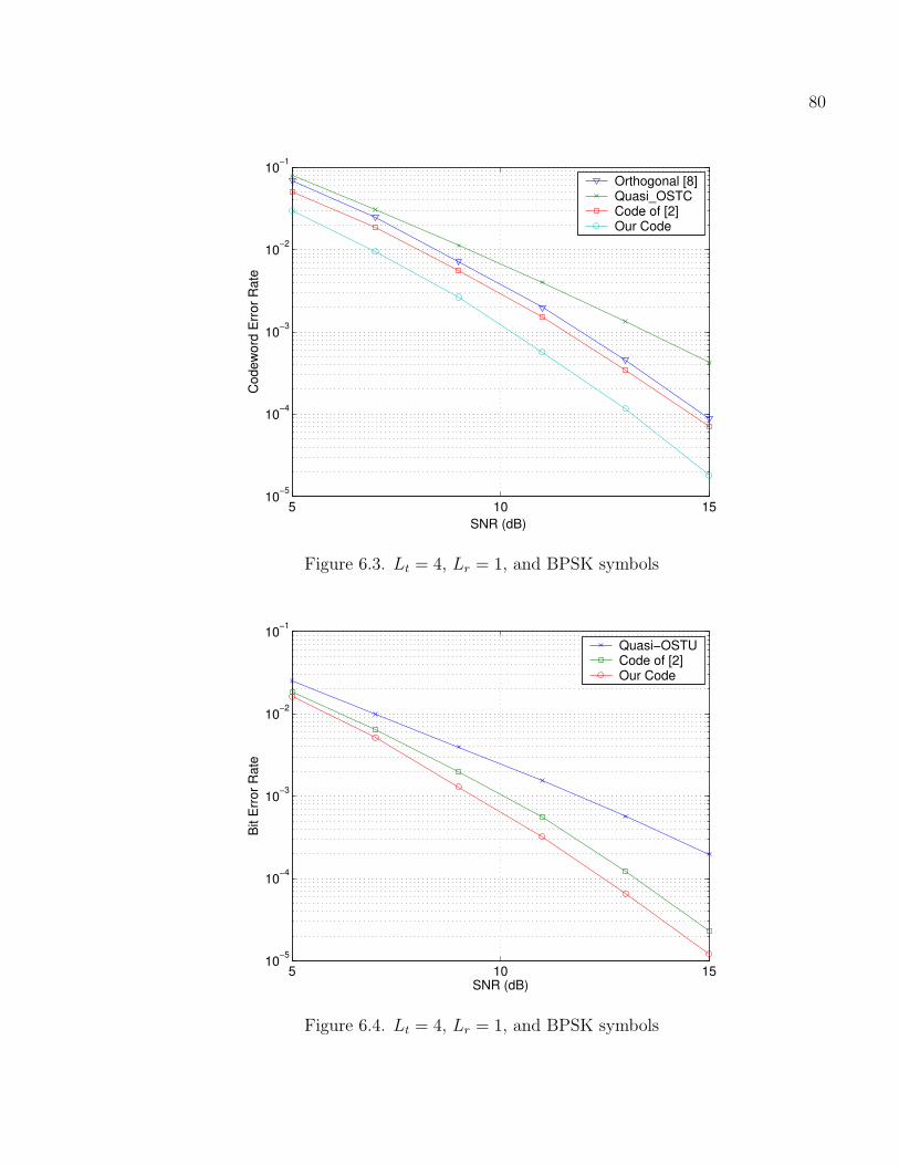
80
5 10 1510−5
10−4
10−3
10−2
10−1
SNR (dB)
Code
word
Erro
r Rat
e
Orthogonal [8]Quasi_OSTCCode of [2]Our Code
Figure 6.3. Lt = 4, Lr = 1, and BPSK symbols
5 10 1510−5
10−4
10−3
10−2
10−1
SNR (dB)
Bit E
rror R
ate
Quasi−OSTUCode of [2]Our Code
Figure 6.4. Lt = 4, Lr = 1, and BPSK symbols

81
10 11 12 13 14 1510−4
10−3
10−2
10−1
SNR (dB)
Fram
e Er
ror R
ate
SQOSTCNew−uncodedquasi−uncoded
Figure 6.5. Lt = 4, Lr = 1, and BPSK symbols, Frame Length=132 channel trans-mission time
5 10 1510−3
10−2
10−1
100
SNR (dB)
Code
word
Erro
r Rat
e
Quasi−OSTCLD−HeathCode of [2]Our Code
Figure 6.6. Lt = 4, Lr = 1, and QPSK symbols

CHAPTER 7
SINGLE-BLOCK CODED MODULATION FOR MIMO SYSTEMS
We propose a new class of space-time coding that provides coding gain without any
outer code or trellis. The new code derives its codewords from block space-time
codes such as orthogonal [34] and quasi orthogonal [36, 39, 40] space-time codes. In
principle, this method can also be applied to any other class of block space-time codes.
Although a space-time block code may provide full diversity and a simple
decoding scheme, they usually do not provide much (if any) coding gain. This is in
contrast to space-time trellis codes [14], which provide full diversity as well as coding
gain but at a cost of higher decoding complexity. Thus there is a natural motivation
to combine better coding gain with the simple decoding offered by STBC. One way
to do so is to build trellises over STBC, and in fact Jafarkhani and Seshadri [42]
and Siwamogsatham and Fitz [44] independently proposed a full rate code which is
a concatenation of an outer trellis code with an inner space-time block code. These
codes were named super-orthogonal codes by [42]. Naturally the outer trellis imposes
some complexity on the decoder.
A natural question at this point would be: why not add coding gain to the
block code itself? One would expect that the methodology of Ungerbock, namely
expanding the constellation size, followed by a careful choice of codewords from the
enlarged constellation, should be applicable to block signaling for MIMO system.
Figure 7.1 shows a figurative idea of how expansion and selection could help to improve
the code performance.
For larger number of antennas and more complicated constellations, it is diffi-
82

83
Original Codewords Expanded Codebook Selected Codewords
Figure 7.1. Expansion and selection idea
cult to systematically perform set partitioning, which is equivalent to selecting code-
words out of expanded constellations, for two reasons: First, by increasing the number
of antennas and constellation dimension, the number of choices increases. For exam-
ple, constellation expansion by a factor of two via QAM in an Lt antenna system
results in a factor of 22Lt expansion in total number of codewords. Second, this ex-
pansion happens in a higher dimensional space, and in general it is not clear how to
systematically approximate centers of packed spheres from the elements of a given
higher-rate lattice in high-dimensional spaces.
However, consider that set partitioning is nothing but a systematic method for
pruning a larger codebook. Even without a systematic set partitioning, one should
still be able to do the pruning. This basic idea is the cornerstone of the developments
in this chapter.
In this chapter, we present a coded modulation technique for space time block
codes. In order to design a code, we employ the existing space-time block codes, e.g.,
orthogonal and quasi-orthogonal block space-time codes (OBSTC and QOBSTC).
Due to decoding simplicity of orthogonal codes, in this chapter we focus on this type
of codes, however the proposed method is general and can be applied to any MIMO
block code, including, e.g., LD and TAST codes. We employ a coding technique
via selection of certain space-time constellation to increase the minimum distance

84
between the codewords. Because our codes do not involve a trellis, their decoding
complexity is smaller than either trellis space-time codes or super-orthogonal codes.
7.1 System Model
The system model consists of a MIMO system with Lt transmit and Lr receive anten-
nas. A flat fading channel is assumed, where the channel gains are constant during
each fade interval and independent in successive intervals. The received signal, de-
noted by a T × Lr matrix R, after matched filtering has the following form:
R =
√
ρ
Lt
SH + N . (7.1)
T represents the number of time slots for transmitting one block of symbols. ρ is the
average received signal-to-noise ratio per antenna. The matrix S is a block space-time
codeword of size T ×Lt. The channel matrix H = {hij} has the size of Lt×Lr where
hij is the fading channel coefficient between jth received antenna and ith transmit
antenna. The AWGN is shown by the matrix N. The receiver employs maximum
likelihood (ML) decoder with perfect knowledge of channel state information.
We use the so-called average union bound (AUB) as the design criterion which
ensures good performance [71]. We introduce AUB below in a manner similar to [69].
PU =1
nc
∑
i,j,i6=j
Pe(ci, cj) (7.2)
where ci and cj are codewords from code S and nc is the total number of codewords
and Pe(ci, cj) is the PEP expression,
Pe(ci, cj)i6=j =1
π
∫ π/2
0
r∏
i=1
(1 +λiρ
4sin2θ)−Lrdθ (7.3)
where r = min(Lt, Lr) and λi are the singular values of
A = (ci − cj)(ci − cj)H .

85
7.2 Code Design
The new code is derived from expurgation of the expanded original code, i.e. our
code utilizes the codewords of the expanded orthogonal space-time code. The expan-
sion is made possible through the use of higher modulation constellation size in the
orthogonal or quasi-orthogonal structure. The resulting expanded code obviously has
more codewords than we need for our desired rate. Then we use pruning to reduce
the number of codewords in a way that the minimum distance of the codebook is
increased, and thus the performance of the code is improved.
We start with an example of Alamouti code [33] using 8PSK constellation. In
this case, we have Lt = 2, and the code is
X2×2 =
(
x1 x2
−x∗2 x∗
1
)
(7.4)
where x1 and x2 are taken from 8PSK constellation. The code consists of 64 code-
words. We can expand the code by switching to 16QAM constellation, which increases
the number of codewords to 256. Then the expanded code can be pruned down by a
factor of four to arrive at a new codebook which has the original rate. The new code
has shown about 0.9dB gain when compared with the original Alamouti code using
8PSK.
The pruning method plays an important role in achieving this gain. We explain
the pruning through two steps. First consider a basic greedy algorithm. We will use
the following notation in the sequel: The basic (original) codebook will be denoted
C, the expanded codebook C ′, and the pruned (optimal) codebook C∗.
The basic algorithm starts by picking a codeword at random from the expanded
orthogonal codebook. We pick the codewords one after another according to distance,
in other words, at each step, we pick the next codeword to be as far as possible from

86
1st codeword
2nd codeword
3rd codeword
4th codeword
Figure 7.2. Incremental codeword selection algorithm. Paths with bad distance prop-erties are terminated.
all previously picked codewords. We continue until the required number of codewords
have been selected from among the expanded codebook.
The basic (greedy) algorithm, however, has a weakness shared by many such
optimization algorithms: it has a tendency of falling into a local minimum. Therefore,
we modify it slightly as follows.
At each step of the algorithm we may have several good choices for codewords
whose minimum distances are not that different. Picking the very best one might
be shortsighted because it may block future options. Therefore, instead of only one,
we consider several codewords as candidates in each step. This will lead to a tree-
based algorithm. Naturally, if we allow the tree to expand indefinitely, the design
complexity will run out of hand. Therefore, at each step, we delete some of the least
attractive paths in the design tree. Without further embellishment, we mention that
this method is similar to discrete optimization methods utilized in some decoding

87
algorithms, however, we omit a complete description of lineage of such algorithms in
the interest of brevity.
Figure 7.2 shows how the code selection process works for the first four code-
words in a hypothetical example. The first codeword is selected randomly. For the
second codeword, we keep a few of the best choices. For each of the possibilities
that are alive, a third codeword is sought, and so on. At each step, the paths that
do not yield attractive distance properties (between so-far selected codewords) are
eliminated. The others are kept alive to allow choices for the future. Experience has
shown that a fully greedy algorithm that keeps only the best codeword at each step,
is too susceptible to local optima.
The performance of the algorithm depends also on a good choice of initial
point. Although it is possible to start from (several) random point(s), a better way
is to do the set partitioning on the original code [42] and pick a set partition as an
initial set. In this way, we are sure that the initial codeword candidates already have
a good distance criterion.
The algorithm consists of simple steps that can be expressed as follows.
1. Select a codeword or a set of codewords as initial set S1,
2. Make new sets by augmenting the sets Si via adding only one codeword from
the expanded code C′,
3. Check the distance of each new normalized sets and only keep the sets that give
minimum PEP,
4. If number of codewords in Si is not sufficient then go to Step 2,
5. All remaining Si are potential new codes.

88
In cases that the expansion is done through non-unit power constellations such
as 16QAM, power normalization should be performed. Although the average power
of the expanded code is unity at each transmission time, but each codeword may have
more or less than unit power at each transmission time. Therefore, we may compare
different sets that have different power level. In order to avoid such a problem, power
normalization can be done for each set at each step of the algorithm.
7.3 Decoding
The key issue at the decoder is to ensure that the simplicity of the decoding is to
some extent maintained. In other words, to ensure that we can still make use of
the structure of the codebook even though it is no longer quite as structured as the
original codebook (due to expurgations). In particular, each orthogonal codeword
consists of elements of a given expanded constellation. The standard decoding process
for orthogonal codes allows the distance metric to be written as a sum of element-
wise metrics, thus simplifying the ML detection. We refer to this construction of the
metric, and the corresponding detection algorithm, as orthogonal decoding [34].
For our new code, we are interested to maintain, as much as possible, the simple
decoding afforded by the orthogonal structure, while achieving the performance of ML
decoding. In general the new codebook C∗ does not by itself present a direct way of
simple ML decoding. However, our knowledge that the codewords of C∗ are also
members of the expanded orthogonal code C ′, can be used to construct an efficient
decoding algorithm.
The decoding algorithm is motivated by the conditioning ideas that have been
used, e.g., in sphere decoding [56]. Consider that each received codeword belongs
to the expanded code. The decoder performs orthogonal decoding according to the
expanded codebook, arriving at a candidate solution. We then check to see if this can-

89
didate is actually a member of the expurgated code. If it is, the decoding is successful.
If it is not a valid codeword, we have no choice but to do a wider search. However,
thankfully the probability of this last event is very small for reasonable codeword
error rates, and thus the average complexity of decoding is minimally impacted by
the last case. The flow of decoding is summarized below.
1. Do orthogonal (quasi-orthogonal) decoding on the expanded codebook C ′, call
the result c.
2. If c ∈ C∗, it is declared the decoded codeword.
3. If c /∈ C∗, look for the other closest points till the closest valid point is found.
The complexity of the wider search, in the unlikely events when it is required,
may be managed by using a list decoding method. The list decoder successively tests
for the second, or third, . . . closest codeword to the received vector, from the expanded
codebook, until a valid codeword in the pruned codebook is found as illustrated in
Figure 7.3. Due to the orthogonal structure of the expanded codebook, each step of
the list decoding is easy.
For the case of orthogonal codes, we propose a simple search method to find
the closest valid codeword to the received point. In this case, the metric for each
symbol is calculated separately. So the detection for every symbol is reduced to a
2-dimensional case.
As an example, consider the general M-QAM constellation. Figure 7.4 shows
a simple scenario of a received point. Similar to the sphere decoding method, the
closest neighbors to the received point has been labeled accordingly. Now we can
pick the first k closest neighbors of each symbols of the codeword. Then the metric

90
can be calculated for all possible combinations of the selected neighbors (= kLt) and
the closet valid point is the ML decoded codeword.
The relative distance to nearby constellation points naturally depends on the
received signal. To arrive at an ordered list of distances, we start from the nearest
constellation point, which was obtained in the first step of decoding. Then, depend-
ing on the location of received vector with respect to that nearest point, we can
systematically list other nearby constellation points in increasing order of distance.
Inspection shows that 8 such lists exist. We divide the area around an MQAM point
into 8 regions, and depending where the receive vector falls with respect to its closest
constellation point, one of these zones is chosen, and the respective list is used. The
idea is that, because these lists have to be calculated and stored only once, the list
itself does not impact the decoding complexity, since its execution is equivalent to a
table-lookup.
Figure 7.5 illustrates the zone assignment for a given constellation point which
is labeled as ij. The table in Figure 7.5 gives the first nine closest neighbors for each
zone. The neighbors are represented as sij where i represents the column and j
represents the row of the given codeword in the QAM constellation structure. It
should be noted that the zones for the border points is less than eight. However, the
ordering in the table is still valid but the neighbors with i or j negative or bigger
than the constellation size should be omitted.
We may also design new codes using quasi-orthogonal codes. Each quasi-
orthogonal codeword consists of two types of sub-matrices, each of them possibly an
orthogonal or quasi-orthogonal codeword of lower dimension. The standard decoding
process for quasi-orthogonal codes allows the distance metric to be written as a sum
of metrics for these two sections, thus simplifying the ML detection. We refer to
this construction of the metric, and the corresponding detection algorithm, as quasi-

91
Figure 7.3. Decoder checks all candidate (expanded) codevectors until a valid code-vector is found.
1
2
3
4
5
7
6
8
9
Figure 7.4. Symbol-wise detection using M-QAM constellation. Labeling shows theorder of the closet constellation points to the received point

92
a
b
c
d e
f
g
h
Zones around each constellation point
i i+1i-1
j
j+1
j-1
Zone n1 n2 n3 n4 n5 n6 , n7 n8 , n9
a sij s(i+1)j si(j−1) s(i+1)(j−1) si(j+1) s(i−1)j , s(i+1)(j+1) s(i−1)(j−1) , s(i+2)j
b sij si(j−1) s(i+1)j s(i+1)(j−1) si(j−1) si(j+1) , s(i−1)(j−1) s(i+1)(j+1) , si(j−2)
c sij si(j−1) s(i−1)j s(i−1)(j−1) s(i+1)j si(j+1) , s(i+1)(j−1) s(i−1)(j+1) , si(j−2)
d sij s(i−1)j si(j−1) s(i−1)(j−1) si(j+1) si(j+1) , s(i−1)(j+1) s(i+1)(j−1) , s(i−2)j
e sij s(i−1)j si(j+1) s(i−1)(j+1) si(j−1) s(i+1)j , s(i−1)(j−1) s(i+1)(j+1) , s(i−2)j
f sij si(j+1) s(i−1)j s(i−1)(j+1) s(i+1)j si(j−1) , s(i+1)(j+1) s(i−1)(j−1) , si(j+2)
g sij si(j+1) s(i+1)j s(i+1)(j+1) s(i−1)j si(j−1) , s(i−1)(j+1) s(i+1)(j−1) , si(j+2)
h sij s(i+1)j si(j+1) s(i+1)(j+1) si(j−1) s(i−1)j , s(i+1)(j−1) s(i−1)(j+1) , s(i+2)j
Figure 7.5. Zone assignment for sij, i and j respectively represent the columns androws of M-QAM constellation and the table shows the neighbors list ordered distance-wise for each zone

93
orthogonal decoding [42]. The decoding algorithm is similar to the orthogonal codes
except the type of decoding.
For the case of quasi-orthogonal codes, we can employ the sphere decoding
method suggested by [72] incorporated in the same decoding algorithm. In cases
that the decoded codeword is a non-valid codeword, the list decoding method can be
applied. It is needed to properly detect the first n neighbors of the received point for
a given reliability. The radius of the sphere for each decoupled metric part can be
determined with regard to the noise power to make sure that we have selected the
required number of neighbors.
7.3.1 Decoding Complexity
We study the decoding complexity along two directions: the average complexity and
the instantaneous complexity. Average complexity, as the name implies, represents
the complexity of decoding averaged over all possible codewords and received vectors.
This gives a rough overall idea about the requirements of the algorithm, and as we
show below, our codes can be decoded in an average complexity that is polynomial
in constellation size. Instantaneous complexity represents the complexity for a given
codeword and receive noise. This is an important factor because any implementation
of the decoding has finite processing power, and real-time processing requires that
if the calculation is not finished within the allowed time, a decoding error must be
issued. The instantaneous complexity is of course a random quantity, and we wish to
understand its distribution.
Average Complexity
Define the expansion factor a as follows
a4=
pe
po
(7.5)

94
where pe = |C ′|, po = |C∗|, and |.| gives the cardinality of the argument.
We assume that our code is designed well, therefore the distance between the
valid codewords are maximized in the space of all codewords, as shown in Figure 7.3.
As shown in the figure, to decode, we can start from the received value and do a list
decoding of successive codewords, moving away from the received value, until a valid
codeword is found. However, the figure also shows that we would visit at most a
codewords in this manner for a typical valid codeword. Each of these visits requires
an orthogonal decoding. Therefore, the overall complexity is represented by a times
a constant, which is independent of the constellation size.
Instantaneous Complexity
We now look at the list decoding mentioned above. We are now interested to see
what is the probability of visiting a certain number of expanded codewords before
arriving at a valid codeword, at which point the decoding terminates.
We note that in many practical scenarios, the closest codeword is a valid
codeword with high probability, therefore the search terminates after the first try. For
example, simulations show that for a 4× 1 system employing a BPSK constellation,
at codeword error rates 10−2 and 10−3 the probability of being forced into a wider
search (after the first try) is less than 0.01 and 0.001 respectively.
Now we calculate an approximation of the probability distribution of list de-
coding length. We know that on average a neighbors are visited, however, for a
given codeword the search depth could be higher or lower. This calculation is needed
because we need to design a receiver such that with high probability, it can accommo-
date the depth of list decoding that is necessary. The following result demonstrates
that the list decoding depth has at worst a geometric probability distribution.

95
Theorem 4 Randomly label po codewords of a code of size pe as valid codewords and
label the rest as invalid. Then if we randomly pick n codewords, the probability of
having at least one valid codeword among them is lower bounded by
1− (1− a−1)n.
Proof: he probability of having no valid codeword in n randomly selected codewords
is
pnv(n) =
(
pe−po
n
)
(
pe
n
) ,
where(
pe
n
)
gives the number of all possible combinations of choosing n from pe. Now
the probability of having at least one valid codeword is
pv(n) = 1− pnv(n)
= 1− (pe − po)(pe − po − 1) · · · (pe − po − n + 1)
pe(pe − 1) · · · (pe − n + 1)
> 1− (pe − po
pe
)n
= 1− (1− a−1)n. (7.6)
�
Since n is in the exponent in (7.6), pv converges to one very fast, however, for
the code selected via our selection algorithm the convergence is even faster over n. The
code selection algorithm tries to separate the codewords as much as possible in the
space in a way that having codewords clustered together is highly unlikely. In other
words, from every a neighbor codewords of C ′
, on average one codeword is valid.
Therefore, many possible outcomes of random selection are ruled out. Figure 7.6
illustrate the lower bound and the exact pv for po = 64 codewords taken from pe = 256
codewords of the expanded code. For instance pv(16) = 0.9915 and pv(25) = 0.9995.
For the example code stated in Table 7.1 which is derived from an Alamouti code

96
using 16-QAM, pv equals to 0.9828, 0.9998 and 1 respectively for n equals to 9, 16
and 25. This means the search for the first 25 neighbors, or in other words the first
5 neighbors for each symbol, gives the exact ML result.
7.4 Simulations
The simulation results are provided for two, three, and four transmit antennas in block
fading. In this chapter, we focus on examples of Lt = 2 and Lt = 3 for orthogonal
codes. However the generalization for higher number of transmit antennas is straight
forward.
Figure 7.7 shows the codeword error rate for the code rate R = 3 bits/Hz/Sec
and two receive antenna system. The original orthogonal code is an Alamouti code
using 8PSK modulation. The code consists of 64 codewords. Our code is a selection
of 64 codewords taken from Alamouti code using 16QAM constellation. A gain of
0.9dB has been obtained over the original Alamouti code.
For the case of Lt = 3 the code is
X4×3 =
x1 x2 x3
−x∗2 x∗
1 0−x∗
3 0 x∗1
0 −x∗3 x∗
2
(7.7)
where x1, x2, and x3 are symbols from the chosen constellation and “∗” denotes the
complex conjugate operator.
Figure 7.8 shows the codeword error rate for the code rate R = 3/4 bits/Hz/Sec.
The original orthogonal codes is a 4× 3 code of (7.7) using BPSK modulation. The
original code consists of 8 codewords. Our codes are a selection of 8 codewords taken
from the code using the same structure but with QPSK and 8PSK constellation. Our
codes derived from 8PSK shows a gain of 1dB and 1.3dB respectively for one- and
two receive antennas.

97
1 5 10 15 20 250.2
0.3
0.4
0.5
0.6
0.7
0.8
0.9
1
n
p v
Exact pvLower bound16−QAM Example
Figure 7.6. Probability of having at least one valid codeword for n closest neighborswhere a = 1/4, po = 64 and pe = 256.
10 12 14 16 18 2010−4
10−3
10−2
SNR (dB)
Bloc
k Er
ror R
ate
Alamouti 8PSKNew out of 16QAM
Figure 7.7. Orthogonal space time codes and expurgated orthogonal code for Lt = 2,T = 2 and rate 3 bits per channel use in slow fading.

98
2 4 6 8 10 1210−3
10−2
10−1
SNR (dB)
Bloc
k Er
ror R
ate
Mr=1, Orthogonal BPSKMr=1, New out of 4QAMMr=1, New out of 8PSKMr=3, Orthogonal BPSKMr=3, New out of 4QAMMr=3, New out of 8PSK
Figure 7.8. Orthogonal space time codes and expurgated orthogonal code for Lt = 3,T = 4 and rate 3/4 bits per channel use in slow fading.
3 4 5 6 7 8 9 10 11
10−4
10−3
10−2
10−1
SNR (dB)
Bloc
k Er
ror R
ate
Mr=1, Modified Quasi, BPSKMr=1, New out of 4QAMMr=2, Modified Quasi, BPSKMr=2, New out of 4QAM
Figure 7.9. Modified quasi-orthogonal space time codes and expurgated codes forLt = 4, T = 4, and rate 1 bits per channel use in slow fading.

99
Table 7.1. New code expressed with the indices of the codewords taken from expandedcode
Code Constellation Lr Indices
X2×2 16-QAM 2 1, 4, 7, 13, 16, 18, 26, 31, 37, 40, 43, 46, 49, 52, 55, 61,64, 66, 72, 74, 85, 87, 92, 93, 97, 99, 105, 111, 120, 122,133, 135, 140, 141, 143, 145, 148, 155, 166, 173, 176, 178,181, 188, 190, 193, 196, 202, 208, 210, 215, 217, 220, 222,227, 229, 232, 239, 241, 244, 247, 250, 253, 256
X4×3 4-QAM 1 1, 7, 9, 15, 35, 37, 43, 45
X4×3 8-PSK 1 1, 21, 107, 160, 293, 305, 335, 444
X4×3 4-QAM 2 1, 7, 9, 15, 35, 37, 43, 45
X4×3 8-PSK 2 1, 21, 107, 160, 293, 305, 335, 444
X4×4 4-QAM 1 1, 11, 35, 41, 88, 94, 118, 128, 131, 137, 161, 171, 214,224, 248, 254
X4×4 4-QAM 2 1, 11, 35, 41, 88, 94, 118, 128, 131, 137, 161, 171, 214,224, 248, 254

100
When Lt = 4, each codeword transmits four symbols at four timing slots.
To design our codes, we start with the modified QOSTC [39], which achieves full
diversity. The modified code applies a constellation rotation either on the first pair
or the second pair of symbols. The code structure is
X4×4 =
ejφx1 ejφx2 x3 x4
e−jφx∗2 e−jφx∗
1 x∗4 x∗
3
x3 x4 ejφx1 ejφx2
x∗4 x∗
3 e−jφx∗2 e−jφx∗
1
(7.8)
where x1, x2, x3, and x4 are symbols from the constellation and φ is the rotation
angle applied on the first pair of symbols. For each φ, matrices X4×4 constitute a
complete quasi-orthogonal codebook. Thus by changing φ we can generate a family
of codebooks.
Figure 7.9 shows the codeword error rate for the code rate R = 1 bits/Hz/Sec.
The original modified quasi-orthogonal codes is a 4 × 4 code of (7.8) using BPSK
modulation. The original code consists of 16 codewords. Our code is a selection of 16
codewords taken from the code using the same structure but with QPSK constellation.
Our code driven from QPSK shows a gain of 1.5dB and 1.8dB respectively for one
and two received antennas at 10−3 block error rate. The optimum rotation for the
original code is set to φ = π/2.
Table 7.1 shows the designed codebook, via indices in the expanded codebook.
We use a simple labeling according to the following convention. Each M -ary constel-
lation is labeled naturally (not Gray) as shown in Figure 7.10. The codeword symbols
are x1, . . . , xN taking values on this constellation. The function label(·) returns the
label of a constellation symbol. The indices of the expanded codebook are calculated
via the following simple expression:
I =N∑
i=1
label(xi) ·MN−i + 1 (7.9)

101
0
1
2
3
0
2
4
6
13
5 70 1 2 3
4-QAM 8-PSK 16-QAM
4 5 6 7
8 9 10 11
12 13 14 15
Figure 7.10. Constellation labeling
7.5 Conclusion
We propose a new space-time code design technique by pruning codewords from an
expanded set of orthogonal space-time codewords. We select the codewords from
the expanded set through an expurgation algorithm. The resulting codes exhibit
attractive coding gains, while maintaining very reasonable decoding complexity.
It is instructive to revisit the varieties of space-time codes designed for diversity
that also provide coding gain. The first type is trellis space-time codes [14], which allow
coding gain but whose complexity is generally higher than block space-time codes.
The second type is the super-orthogonal codes of [42, 44] which are constructed by
expanding block codebooks (e.g. Alamouti) and building trellises on them. The third
type consists of codes presented in this chapter, which incorporate coding gain into
the block code itself. Because they do not involve a trellis, their decoding complexity
is smaller than either [14] or [42, 44].

REFERENCES
[1] H. Jafarkhani, Space-time coding: Theory and practice, Cambridge University
Press, 1st edition, 2005.
[2] D. Gesbert, M. Shafi, D. Shiu, P. J. Smith, and A. Naguib, “From theory to
practice: An overview of MIMO space-time coded wireless systems,” IEEE J.
Select. Areas Commun., vol. 21, no. 3, pp. 281–302, Apr. 2003.
[3] G. J. Foschini and M. J. Gans, “On limits of wireless communications in a fading
environment when using multiple antennas,” Wireless Pres. Commun., vol. 6,
pp. 311–335, Mar. 1998.
[4] G. J. Foschini, “Layered space-time architecture for wireless communication
in a fading environment when using multielement antennas,” Bell Labs. Tech.
Journal, vol. 2, pp. 41–59, Autumn 1996.
[5] E. Telatar, “Capacity of multiantenna gaussian channels,” AT&T Bell Labora-
tories, Tech. Memo, June 1995.
[6] G. Raleigh and J. M. Cioffi, “Spatial-temporal coding for wireless communica-
tions,” IEEE Transactions on Communications, vol. 46, pp. 357–366, 1998.
[7] H. Bolcskei, D. Gesbert, and A. J. Paulraj, “On the capacity of OFDM based
spatial multiplexing systems,” IEEE Transactions on Communications, vol. 50,
no. 2, pp. 225–234, Feb. 2002.
[8] A. J. Paulraj and T. Kailath, “Increasing capacity in wireless broadcast systems
using distributed transmission/directional reception,” Patent 5 345 599, 1994.
102

103
[9] J. H. Winters, “On the capacity of radio communication systems with diversity
in a Rayleigh fading environment,” IEEE J. Select. Areas Commun., vol. SAC-5,
pp. 871–878, June 1987.
[10] G. D. Golden, G. J. Foschini, R. A. Valenzuela, and P. W. Wolniansky, “Detec-
tion algorithm and initial laboratory results using the v-blast space-time com-
munication architecture,” IEE Electronics Letters, vol. 35, no. 1, pp. 14–15,
1999.
[11] G. J. Foschini, G. D. Golden, R. A. Valenzuela, and P. W. Wolniansky, “Sim-
plified processing for high spectral efficiency wireless communication employing
multi-element arrays,” IEEE Journal on Selected Areas in Communications, vol.
17, pp. 1841 1852, Nov. 1999.
[12] N. Seshadri and J. H. Winters, “Two schemes for improving the performance
of frequency-division duplex (FDD) transmission systems using transmitter an-
tenna diversity,” Int. J. Wireless Information Networks, vol. 1, pp. 49–60, jan
1994.
[13] A. Wittneben, “A new bandwidth efficient transmit antenna modulation diver-
sity scheme for linear digital modulation,” Proc. IEEE ICC, vol. 3, pp. 1630–
1634, 1993, Geneva, Switzerland.
[14] V. Tarokh, N. Seshardi, and A.R. Calderbank, “Space-time codes for high
data rate wireless communications: Performance criteria and code construction,”
IEEE Transactions on Information Theory, vol. 44, no. 2, pp. 744–765, Mar.
1998.
[15] B. Hassibi and B. Hochwald, “High-rate codes that are linear in space and time,”
IEEE Transactions on Information Theory, vol. 48, no. 7, pp. 1804–1824, July
2002.

104
[16] R.W. Heath and A. J. Paulraj, “Linear dispersion codes for mimo systems based
on frame theory,” IEEE Transactions on Signal Processing, vol. 50, no. 10, pp.
2429–2441, Oct. 2002.
[17] I. E. Telatar, “Capacity of multiantenna gaussian channels,” Eur. Trans. Com-
mun., vol. 10, no. 6, pp. 585–595, 1999.
[18] J. W. Silverstein, “Strong convergence of the empirical distribution of eigenvalues
of large dimensional random matrices,” J. Multivariate Anal., vol. 55, no. 2, pp.
331–339, 1995.
[19] P. B. Rapajic and D. Popescu, “Information capacity of a random signature
multiple-input multiple-output channel,” IEEE Transactions on Communica-
tions, vol. 48, pp. 1245–1248, Aug. 2000.
[20] A. Lozano, F. R. Farrokhi, and R. A. Valenzuela, “Lifting the limits on high-
speed wireless data access using antenna arrays,” IEEE Communications Mag-
azine, vol. 39, pp. 156–162, Sep. 2001.
[21] P. F. Driessen and G. J. Foschini, “On the capacity formula for multiple- input
multiple-output wireless channels: A geometric interpretation,” IEEE Transac-
tions on Communications, vol. 47, pp. 173–176, Feb. 1999.
[22] D. Shiu, “Wireless communication using dual antenna arrays,” ser. Interna-
tional Series in Engineering and Computer Science. Norwell, MA: Kluwer, 1999.
[23] F. R. Farrokhi, G. J. Foschini, A. Lozano, and R. A. Valenzuela, “Linkopti-
mal space-time processing with multiple transmit and receive antennas,” IEEE
Communicatons Letters, vol. 5, pp. 85–87, 2001.

105
[24] C. N. Chuah, D. Tse, J. M. Kahn, and R.Valenzuela, “Capacity scaling in mimo
wireless systems under correlated fading,” IEEE Transactions on Information
Theory, vol. 48, pp. 637–650, Mar. 2002.
[25] J. G. Proakis, Digital Communications, New York: McGraw-Hill, 3rd edition,
1995.
[26] M. P. Fitz and J. V. Krogmeier, “Further results on space-time codes for Rayleigh
fading,” Proc Allerton, pp. 391–400, Sep. 1998.
[27] Q. Yan and R. S. Blum, “Optimum space-time convolutional codes for quasi-
static slow fading channels,” Proc. IEEE WCNC, pp. 1351–1355, Sep. 2000.
[28] S. Baro, G. Bauch, and A. Hansmann, “Improved codes for space-time trellis-
coded modulation,” IEEE Communicatons Letters, vol. 46, pp. 524–542, Jan.
2000.
[29] A. R. Hammons and H. E. Gamal, “On the theory of space-time codes for PSK
modulation,” IEEE Transactions on Information Theory, vol. 46, pp. 524–542,
Mar. 2000.
[30] Z. Chen, J. Yuan, and B. Vucetic, “Improved space-time trellis coded modulation
scheme on slow fading channels,” Proc. IEEE ISIT, 2001.
[31] Y. Liu, M. P. Fitz, and O. Y. Takeshita, “A rank criterion for QAM space-time
codes,” Proc. IEEE ISIT, pp. 3062–3079, Dec. 2000.
[32] J. Yuan, Z. Chen, B. Vucetic, and W. Firmanto, “Performance and design of
space-time coding in fading channels,” IEEE Trans. Commun., vol. 51, no. 12,
pp. 1991–1996, Dec. 2003.

106
[33] S. M. Alamouti, “A simple transmit diversity technique for wireless communi-
cations,” IEEE J. Select. Areas Commun., vol. 16, no. 8, pp. 1451–1458, Oct.
1998.
[34] V. Tarokh, H. Jafarkhani, and A.R. Calderbank, “Space-time block codes from
orthogonal designs,” IEEE Transactions on Information Theory, vol. 45, no. 5,
pp. 1456–1467, July 1999.
[35] G. Ganesan and P. Stoica, “Space-time diversity using orthogonal and amicable
orthogonal designs,” Wireless Personal Communications, pp. 165–178, Aug.
2001.
[36] H. Jafarkhani, “A quasi-orthogonal space-time code,” IEEE Trans. Commun.,
vol. 49, no. 1, pp. 1–4, Jan. 2001.
[37] D. Aktas and M. P. Fitz, “Distance spectrum analysis of space-time trellis-
codded modulations in quasi-static Rayleigh fading channels,” IEEE Transac-
tions on Information Theory, vol. 49, no. 12, pp. 3335–3344, Dec. 2003.
[38] H. Jafarkhani and N. Hassanpour, “Super quasi-orthogonal space-time trellis
codes for four transmit antennas,” IEEE Transactions on Wireless Communi-
cations, vol. 4, no. 1, pp. 215–227, Jan. 2005.
[39] N. Sharma and C. B. Papadias, “Improved quasi-orthogonal codes through con-
stellation rotation,” IEEE Trans. Commun., vol. 51, no. 3, pp. 563–571, Mar.
2003.
[40] W. Su and X. Xia, “Signal constellations for quasi-orthogonal space-time block
codes with full diversity,” IEEE Transactions on Information Theory, vol. 50,
no. 10, pp. 2331–2347, Oct. 2003.

107
[41] O. Tirkkonen, “Optimizing space-time block codes by constellation rotations,”
Finnish Wireless Communications Workshop, Oct. 2001.
[42] H. Jafarkhani and N. Seshadri, “Super-orthogonal space-time trellis codes,”
IEEE Transactions on Information Theory, vol. 49, no. 4, pp. 937–950, Apr.
2003.
[43] D. M. Ionescu, K. K. Mukkavilli, Z. Yan, and J. Lilleberg, “Improved 8-state
and 16-state space-time codes for 4-PSK with two transmit antennas,” IEEE
Communicatons Letters, vol. 5, no. 7, pp. 301–303, July 2001.
[44] S. Siwamogsatham and M. P. Fitz, “Improved high-rate space-time codes via
orthogonality and set partitioning,” Proc. IEEE WCNC, vol. 1, pp. 264–270,
Mar. 2002.
[45] G. Ungerbock, “Channel coding with multilevel/phase signals,” IEEE Trans.
Inform. Theory, vol. 28, no. 1, pp. 55–67, Jan. 1987.
[46] S. Alamouti, V. Tarokh, and P. Poon, “Trellis-coded modulation and trans-
mit diversity: design criteria and performance evaluation,” IEEE International
Conference on Universal Personal Communication, vol. 2, pp. 917–920, 1998.
[47] Jr. G. J. Foschini, M. J. Gans D. Chizhik, C. Papadias, and R. A. Valenzuela,
“Analysis and performance of some basic space-time architectures,” IEEE J.
Select. Areas Commun., vol. 21, no. 3, pp. 303–320, Apr. 2003.
[48] M. Grotschel, L. Lovsz, and A. Schriver, Geometric Algorithms and Combinato-
rial Optimization, New York: Springer-Verlag, 2nd edition, 1993.
[49] B. Hassibi, “An efficient square-root algorithm for BLAST,” submitted for
publication in IEEE Trans. on Signal Processing, 2006.

108
[50] M. O. Damen, A. Chkeif, and J. C. Belfiore, “Lattice code decoder for space-time
codes,” IEEE Communicatons Letters, vol. 4, no. 5, pp. 161–163, May 2000.
[51] R. Kannan, “Improved algorithms on integer programming and related lattice
problems,” Proc of 15th annu. ACM Symp. Theory Comput., pp. 193–206, 1983.
[52] J. Lagarias, H. Lenstra, and C. Schnorr, “Korkin-Zolotarev bases and successive
minima of a lattice and its reciprocal,” Combinatorica, vol. 10, pp. 333–348,
1990.
[53] A. Korkin and G. Zolotarev, “Sur les formes quadratiques,” Math Annu., vol.
6, pp. 366–389, 1873.
[54] M. Pohst, “On the computation of lattice vectors of minimal length, successive
minima and reduced basis with applications,” ACM SIGSAM Bull, vol. 15, pp.
37–44, 1981.
[55] B. Hassibi and H. Vikalo, “On the sphere-decoding algorithm I. expected com-
plexity,” IEEE Transactions on Signal Processing, vol. 53, no. 8, pp. 2806–2818,
Aug. 2005.
[56] U. Fincke and M. Pohst, “Improved methods for calculating vectors of short
length in a lattice, including a complexity analysis,” Math Comput., vol. 44, pp.
463–471, Apr. 1985.
[57] R. H. Gohari and T. N. Davidson, “Design of linear dispersion codes: Asymptotic
guidelines and their implementation,” IEEE Transactions on Wireless Commu-
nications, vol. 4, no. 6, pp. 2892–2908, Nov. 2005.
[58] H. El-Gamal and Jr. A. R. Hammons, “A new approach to layered space-time
coding and signal processing,” IEEE Transactions on Information Theory, vol.
47, no. 6, pp. 2321–2334, Sep. 2001.

109
[59] H. El-Gamal and M. Oussama Damen, “Universal space-time coding,” IEEE
Transactions on Information Theory, vol. 49, no. 5, pp. 1097–1119, May 2003.
[60] M. O. Damen, H. El-Gamal, and N. C. Beaulieu, “Linear threaded algebraic
space-time consteloldlations,” IEEE Transactions on Information Theory, vol.
49, no. 10, pp. 2372–2388, Oct. 2003.
[61] X. Giraud, E. Boutillon, and J. C. Belfiore, “Algebraic tolls to build modulation
schemes for fading channels,” IEEE Transactions on Information Theory, vol.
43, pp. 938–952, May 1997.
[62] E. Viterbo and J. Boutros, “Universal lattice code decoder for fading channel,”
IEEE Transactions on Information Theory, vol. 45, pp. 1639–1642, Jul. 1999.
[63] M. O. Damen, K. Abed-Meraim, and M. S. Lemdani, “Further results on the
sphere decoder,” Proc. IEEE ISIT, p. 333, June 2001, Washington, DC.
[64] J. C. Belfiore and G. Rekaya, “Quaternionic lattices for space-time coding,”
Proc. Information Theory Workshop, pp. 267–270, Mar. 2003, Paris, France.
[65] A. R. Calderbank, S. Diggavi, S.Das, and N. Al-Dhahir, “Construction and
analysis of a new 4 × 4 orthogonal space-time block code,” Proc. IEEE ISIT,
June 2004, Chicago, USA.
[66] G. Ungerboeck, “Trellis-coded modulation with redundant signal sets part II:
state of the art,” IEEE Communications Magazine, vol. 25, no. 2, pp. 12–21,
Feb. 1987.
[67] W. F. de la Vega, M. Karpinski, C. Kenyon, and Y. Rabani, “Approximation
schemes for clustering problems,” Annual ACM Symposium on Theory of Com-
puting, pp. 50–55, 2003.

110
[68] W. F. de la Vega, M. Karpinski, and C. Kenyon, “A polynomial time approxi-
mation scheme for metric min-bisection,” Electronic Colloquim on Computional
Complexity, , no. 41, pp. 1–12, 2002.
[69] M. K. Byun and B. Gi Lee, “New bounds of pairwise error probability for space-
time codes in Rayleigh fading channels,” Proc. IEEE WCNC, vol. 1, pp. 89–93,
Mar. 2002.
[70] M. Janani and A. Nosratinia, “Generalized block space-time trellis codes: set
parttioning and code design,” Proc. IEEE WCNC, pp. 461–465, Mar. 2005.
[71] M. Janani and A. Nosratinia, “Relaxed threaded space-time codes,” in Proc.
IEEE GLOBECOM, St. Louis, MO, Nov. 2005.
[72] A. Y. Peng, I.-M. Kim, and S. Yousefi, “Low-complexity sphere decoding al-
gorithm for quasi-orthogonal space-time block codes,” IEEE Transactions on
Communications, vol. 54, no. 3, pp. 377–382, Mar. 2006.

VITA
Mohammad Janani was born in Tehran, Iran, in 1972, the son of Ali Janani and
Razieh Fotouhi. He received the degree of Bachelor of Science in Electrical Engineer-
ing from Amirkabir University of Technology, Tehran, Iran, in 1994 and the degree
of Master of Science in Electrical Engineering from Iran University of Science and
Technology in 1998. In January 2001 he began working toward the Ph.D. degree in
Electrical Engineering in The University of Texas at Dallas.
Permanent address: No 19, Ghanbari Lane, Shamshiri St., Tehran 13838, Iran