constructingelliptic curveisogenies in quantum ... · constructingelliptic curveisogenies in...

arX

iv:1

012.

4019

v3 [

quan

t-ph

] 1

6 A

pr 2

018

Constructing elliptic curve isogenies

in quantum subexponential time

Andrew M. Childs1,2, David Jao1, and Vladimir Soukharev1

1 Department of Combinatorics and Optimization,University of Waterloo, Waterloo, Ontario, N2L 3G1, Canada

2 Institute for Quantum Computing,University of Waterloo, Waterloo, Ontario, N2L 3G1, Canada

amchilds,djao,[email protected]

Abstract. Given two elliptic curves over a finite field having the same cardinality and en-domorphism ring, it is known that the curves admit an isogeny between them, but findingsuch an isogeny is believed to be computationally difficult. The fastest known classical al-gorithm takes exponential time, and prior to our work no faster quantum algorithm wasknown. Recently, public-key cryptosystems based on the presumed hardness of this problemhave been proposed as candidates for post-quantum cryptography. In this paper, we give asubexponential-time quantum algorithm for constructing isogenies, assuming the GeneralizedRiemann Hypothesis (but with no other assumptions). Our algorithm is based on a reductionto a hidden shift problem, together with a new subexponential-time algorithm for evaluatingisogenies from kernel ideals (under only GRH), and represents the first nontrivial applicationof Kuperberg’s quantum algorithm for the hidden shift problem. This result suggests thatisogeny-based cryptosystems may be uncompetitive with more mainstream quantum-resistantcryptosystems such as lattice-based cryptosystems.

1 Introduction

We consider the problem of constructing an isogeny between two given isogenous ordinary ellipticcurves defined over a finite field Fq and having the same endomorphism ring. (Two such curves arecalled horizontally isogenous.) This problem has led to several applications in elliptic curve cryp-tography, both constructive and destructive. The fastest known probabilistic algorithm for solvingthis problem is the algorithm of Galbraith and Stolbunov [18], based on the work of Galbraith,Hess, and Smart [17]. Their algorithm is exponential, with a worst-case (and average-case) runningtime roughly proportional to 4

√q.

Although quantum attacks are known against several cryptographic protocols of an algebraicnature [12, 19, 34], until now there has been no nontrivial quantum algorithm for constructingisogenies. The difficulty of this problem has led to various constructions of public-key cryptosystemsbased on finding isogenies, beginning with a proposal of Couveignes [10]. More recently, Rostovtsevand Stolbunov [29] and Stolbunov [36] proposed refined versions of these cryptosystems with thespecific aim of obtaining cryptographic protocols that resist attacks by quantum computers.

In this work, we give a subexponential-time quantum algorithm for constructing an isogenybetween two given horizontally isogenous elliptic curves, and show that the running time of our

algorithm is bounded above by Lq(12 ,

√32 ) under (only) the Generalized Riemann Hypothesis (GRH).

This result raises serious questions about the viability of isogeny-based cryptosystems in the context

http://arxiv.org/abs/1012.4019v3

2 Andrew M. Childs, David Jao, and Vladimir Soukharev

of quantum computers. At present, isogeny-based cryptosystems are not especially attractive sincetheir performance is poor compared to other quantum-resistant cryptosystems, such as lattice-based cryptography [20]. Nevertheless, they represent a distinct family of cryptosystems worthyof analysis (for reasons of diversity if nothing else, given the small number of quantum-resistantpublic-key cryptosystem families available [27]). Since isogeny-based cryptosystems already performpoorly at moderate security levels [36, Table 1], any improved attacks such as ours would seem todisqualify such systems from consideration in a post-quantum world.

1.1 Contributions

Our first main contribution, described in Section 5, is a reduction from the problem of isogenyconstruction to the abelian hidden shift problem. While a connection between isogenies and hiddenshifts was noted previously by Stolbunov [36], we observe that the reduction gives an injective hiddenshift problem. This allows us to apply an algorithm of Kuperberg [25] to solve the hidden shiftproblem using a subexponential number of queries to certain functions. This reduction constitutesthe first nontrivial application of Kuperberg’s algorithm outside of the black-box setting.

The reduction to the hidden shift problem alone does not immediately give a subexponential-time algorithm for computing isogenies, because one must consider the time required to compute thehiding functions. Indeed, prior to our work there was no known subexponential-time algorithm toevaluate these functions. Our second main contribution, described in Section 4, is a subexponential-time (classical) algorithm to compute the isogeny star operator, which is defined as a certain actionof an ideal class group on a set of elliptic curves. In this way we can compute the hiding functions insubexponential time and thus obtain a subexponential-time reduction to the hidden shift problem.Unlike previous algorithms for isogeny computation [16, 17, 23], our runtime analysis assumes onlyGRH, whereas all previous subexponential-time algorithms for isogeny problems have requiredadditional heuristic assumptions. We achieve this improvement using expansion properties of acertain Cayley graph [22]. The same idea can also be used to obtain subexponential algorithms(under only GRH) for evaluating isogenies (see Remark 4.9). In addition, Bisson [4] has shownthat our method yields a subexponential algorithm for computing endomorphism rings of ordinaryelliptic curves under GRH.

Kuperberg’s algorithm for the abelian hidden shift problem uses superpolynomial space (i.e., aquantum computer with superpolynomially many qubits), so the same is true of the most straight-forward version of our algorithm. Since it is difficult to build quantum computers with many qubits,this feature could limit the applicability of our result. However, we also obtain an algorithm usingpolynomial space by taking advantage of an alternative approach to the abelian hidden shift prob-lem due to Regev [28]. Regev only explicitly considered the case of the hidden shift problem in acyclic group whose order is a power of 2, and even in that case did not compute the constant inthe exponent of the running time. We fill both of these gaps in our work, showing that the hiddenshift problem in any finite abelian group A can be solved in time L|A|(

12 ,√2) by a quantum com-

puter using only polynomial space. Consequently, we give a polynomial-space quantum algorithm

for isogeny construction using time Lq(12 ,

√32 +

√2). The group relevant to isogeny construction is

not always cyclic, so the extension to general abelian groups is necessary for our application.

1.2 Related work

Our algorithm for evaluating the isogeny star operator is based on reducing an ideal modulo prin-cipal ideals to obtain a smooth ideal. This idea is originally due to Galbraith, Hess, and Smart [17].

Constructing elliptic curve isogenies in quantum subexponential time 3

Broker, Charles, and Lauter [7] and Jao and Soukharev [23] also use this idea to give algorithmsfor evaluating isogenies. Bisson and Sutherland [5] use a similar smoothing technique to computeendomorphism rings in subexponential time. We stress that, with the exception of [7], which is re-stricted in scope to small discriminants, all the results mentioned above make heuristic assumptionsof varying severity [5, §4][17, p. 37][23, p. 224] in addition to the Generalized Riemann Hypothesisin the course of proving their respective runtime claims. Our work is the first to achieve provablysubexponential running time with no heuristic assumptions other than GRH. In practice, the heuris-tic algorithms in [5] and [23] run slightly faster than our algorithms in Section 4, because they makeuse of an optimized exponent distribution (originating from [5]) that minimizes the number of largedegree isogenies appearing in the smooth factorization. Our work does not use this optimization,because doing so would reintroduce the need for additional heuristic assumptions.

An alternative approach to computing isogenies, given in Couveignes [10, p. 11] and Stol-bunov [36, p. 227], is to treat the class group as a Z-module and use lattice basis reduction tocompute the isogeny star operator. In practice, the lattice-based approach works well for moder-ate parameter sizes. However, since it amounts to solving the closest vector problem, the methodasymptotically requires exponential time (even with known quantum algorithms), and thus is slowerthan our approach.

2 Isogenies

For general background on elliptic curves, we refer the reader to Silverman [35].Let E and E′ be elliptic curves defined over a field F . An isogeny φ : E → E′ is an algebraic

morphism satisfying φ(∞) = ∞. The degree of an isogeny is its degree as an algebraic map. Theendomorphism ring End(E) is the set of isogenies from E(F ) to itself. This set forms a ring underpointwise addition and composition.

When F is a finite field, the rank of End(E) as a Z-module is either 2 or 4. We say E issupersingular if the rank is 4, and ordinary otherwise. A supersingular curve cannot be isogenous toan ordinary curve. Most elliptic curves are ordinary (in particular, supersingular curves have densityzero [32]), and most current proposals for isogeny-based cryptography (including all publishedisogeny-based public-key cryptosystems) use ordinary curves. Thus, in this paper we restrict ourattention to ordinary elliptic curves. It remains an interesting open problem to study cryptographicapplications of isogenies between supersingular curves and to better understand the computationaldifficulty of computing such isogenies, but we do not address this issue.

Over a finite field Fq, two elliptic curves E and E′ are isogenous if and only if #E(Fq) =#E′(Fq) [37]. The endomorphism ring of an ordinary elliptic curve over a finite field is an imaginaryquadratic order O∆ of discriminant ∆ < 0. The set of all isomorphism classes (over Fq) of isogenouscurves with endomorphism ring O∆ is denoted Ellq,n(O∆), where n is the cardinality of any suchcurve. We represent elements of Ellq,n(O∆) by taking the j-invariant of any representative curve inthe isomorphism class.

An isogeny between two curves having the same endomorphism ring is called a horizontalisogeny [15]. Likewise, we say that two isogenous curves are horizontally isogenous if their endomor-phism rings are equal. Any separable horizontal isogeny φ : E → E′ between curves in Ellq,n(O∆)can be specified, up to isomorphism, by giving E and kerφ [35, III.4.12]. The kernel of an isogeny,in turn, can be represented as an ideal in O∆ [39, Thm. 4.5]. Denote by φb : E → Eb the isogenycorresponding to an ideal b (keeping in mind that φb is only defined up to isomorphism of Eb).Principal ideals correspond to isomorphisms, so any other ideal equivalent to b in the ideal class


group Cl(O∆) of O∆ induces the same isogeny, up to isomorphism [39, Thm. 3.11]. Hence oneobtains a well-defined group action

∗ : Cl(O∆)× Ellq,n(O∆) → Ellq,n(O∆)

[b] ∗ j(E) = j(Eb)

where [b] denotes the ideal class of b. This group action, which we call the isogeny star operator, isfree and transitive [39, Thm. 4.5], and thus Ellq,n(O∆) forms a principal homogeneous space overCl(O∆).

Isogeny graphs under GRH

Our runtime analysis in Section 4 relies on the following result of [22] which states, roughly, that ran-dom short products of small primes in Cl(O∆) yield nearly uniformly random elements of Cl(O∆),under GRH.

Theorem 2.1. Let O∆ be an imaginary quadratic order of discriminant ∆ < 0 and conductor c.Set G = Cl(O∆). Let B and x be real numbers satisfying B > 2 and x ≥ (ln |∆|)B . Let Sx be themultiset A ∪ A−1 where

A = [p] ∈ G : gcd(c, p) = 1 and N(p) ≤ x is prime

with N(p) denoting the norm of p. Then, assuming GRH, there exists a positive absolute constantC > 1, depending only on B, such that for all ∆, a random walk of length

t ≥ Cln |G|

ln ln |∆|in the Cayley graph Cay(G,Sx) from any starting vertex lands in any fixed subset S ⊂ G with

probability at least 12|S||G| .

Proof. Apply Corollary 1.3 of [22] with the parameters

– K = the field of fractions of O∆

– G = Cl(O∆)– q = |∆|.

Following [11], we refer to G = Cl(O∆) as the ring class group of ∆. Observe that by Remark 1.2(a)of [22], Corollary 1.3 of [22] applies to the ring class group G, since ring class groups are quotients ofnarrow ray class groups [11, p. 160]. By Corollary 1.3 of [22], Theorem 2.1 holds for all sufficientlylarge values of |∆|, i.e., for all but finitely many |∆|. To prove the theorem for all |∆|, simply takea larger (but still finite) value of C.

Corollary 2.2 Theorem 2.1 still holds with the set A redefined as

A = [p] ∈ G : gcd(m∆, p) = 1 and N(p) ≤ x is prime

where m is any integer having at most O(x1/2−ε log |∆|) prime divisors.

Proof. The alternative definition of the set A differs from the original definition by no more thanO(x1/2−ε log |∆|) primes. As stated in [22, p. 1497], the contribution of these primes can be absorbedinto the error term O(x1/2 log(x) log(xq)), and hence does not affect the conclusion of the theorem.


3 The group action inverse problem

For a fixed discriminant ∆, the vectorization [10, §2] or group action inverse [36, §2.4] problem isthe problem of finding an ideal class [b] ∈ Cl(O∆) such that [b] ∗ j(E) = j(E′), given j(E) andj(E′). We refer to [b] as the quotient of j(E) and j(E′). The computational infeasibility of findingquotients in Ellq,n(O∆) is a necessary condition for the security of isogeny-based cryptosystems [10,§3][36, §7]. In the remainder of this paper, we present our subexponential algorithm for evaluatingquotients in Ellq,n(O∆) on a quantum computer.

A notable property of isogeny-based cryptosystems is that they do not require the ability toevaluate the isogeny star operator efficiently on arbitrary inputs. It is enough to sample from randomsmooth ideals (for which ∗ can be evaluated efficiently) when performing operations such as keygeneration [10, §5.4][36, §6.2]. However, to attack these cryptosystems using our approach, we dorequire the ability to evaluate the isogeny star operator on arbitrary inputs. We turn to this problemin the next section.

4 Computing the isogeny star operator

In this section, we describe a new classical (i.e., non-quantum) algorithm to evaluate the isogenystar operator. All notation is as in Section 2. Given an ideal class [b] in Cl(O∆), and a j-invariantE of an ordinary elliptic curve of endomorphism ring O∆ over Fq, we wish to evaluate [b] ∗ j(E).We define

LN (12 , c) := exp[(c+ o(1))√lnN ln lnN ].

For convenience, we denote Lmax|∆|,q(12 , c) by L(c).

In Section 4.1 we show that, under GRH, our algorithm has a running time of Lq(12 ,

√32 ), which is

subexponential in the input size. For clarity, we present our algorithms and analysis in full instead ofas “patches” to existing work. We emphasize that the basic structure of these algorithms appearedin prior work; our main contribution is to the analysis, which is facilitated by small changes tothe algorithms. Specifically, Algorithm 1 is based on [23, Algorithm 3], which is in turn based onSeysen’s algorithm [33]; Algorithm 2 is based on [7, Algorithm 4.1]. Our bounds on t in Algorithm 1are new, and allow us to prove the crucial runtime bound (Proposition 4.3).

Computing a relation. Given an ideal class [b] ∈ Cl(O∆), Algorithm 1 produces a relation vectorz = (z1, . . . , zf ) ∈ Z

f for [b], with respect to a factor base F = p1, . . . , pf, satisfying [b] = Fz :=pz11 · · · pzff , with the additional property (cf. Proposition 4.5) that the L1-norm |z|1 of z is less than

O(ln |∆|) for some absolute implied constant (here the L1 norm of a vector denotes the sum of theabsolute values of its coordinates). Algorithm 1 is similar to Algorithm 11.2 in [8], except that weimpose a constraint on |v|1 in Step 5 in order to keep |z|1 small, and (for performance reasons)we use Bernstein’s algorithm instead of trial division to find smooth elements. We remark thatCorollary 9.3.12 of [8] together with the restriction C > 1 in Theorem 2.1 implies that there existsa value of t satisfying the inequality in Algorithm 1.

Computing j(E′). Algorithm 2 is the main algorithm for evaluating the isogeny star operator.It takes as input a discriminant ∆ < 0, an ideal class [b] ∈ Cl(O∆), and a j-invariant j(E) ∈Ellq,n(O∆), and produces the element j(E′) ∈ Ellq,n(O∆) such that [b] ∗ j(E) = j(E′). Eliminating


Algorithm 1 Computing a relation

Input: ∆, q, n, z, [b], and an integer t satisfying C ln |Cl(O∆)|ln ln |∆|

≤ t ≤ C ln |∆| where C is the constant of

Theorem 2.1/Corollary 2.2Output: A relation vector z ∈ Z

f such that [b] = [Fz], or nil1: Compute a factor base consisting of split primes; discard any primes dividing qn to obtain a new factor

base F = p1, p2, . . . , pf2: Set S ← ∅, P ← N(p) : p ∈ F3: Set ℓ← L( 1

4z)

4: for i = 0 to ℓ do5: Select v ∈ Z

f0..|∆|−1 uniformly at random subject to the condition that |v|1 = t

6: Calculate the reduced ideal av in the ideal class [b] · [Fv]7: Set S ← S ∪N(av)8: end for

9: Using Bernstein’s algorithm [3], find a P-smooth element N(av) ∈ S (if one exists), or else return nil

10: Find the prime factorization of the integer N(av)11: Using Theorem 3.1 of Seysen [33] on the prime factorization of N(av), factor the ideal av over F to

obtain av = Fa for some a ∈ Zf

12: Return z = a− v

Algorithm 2 Computing j(E′)

Input: ∆, q, [b], and a j-invariant j(E) ∈ Ellq,n(O∆)Output: The element j(E′) ∈ Ellq,n(O∆) such that [b] ∗ j(E) = j(E′)1: Using Algorithm 1 with any valid choice of t, compute a relation z ∈ Z

f such that [b] = [Fz] =[pz11 p

z22 · · · p

zff ]

2: Compute a sequence of isogenies (φ1, . . . , φs) such that the composition φc : E → Ec of the sequencehas kernel E[pz11 p

z22 · · · p

zff ], using the method of [7, §3]

3: Return j(Ec)

the primes dividing qn is necessary for the computation of the isogenies in the final step of thealgorithm.

Algorithm 2 is correct since the ideals b and Fz belong to the same ideal class, and thus actidentically on Ellq,n(O∆).

4.1 Runtime analysis

Here we determine the theoretical running time of Algorithm 2, as well as the optimal value ofthe parameter z in Algorithm 1. As is typical for subexponential-time factorization algorithmsinvolving a factor base, these two quantities depend on each other, and hence both are calculatedsimultaneously.

Proposition 4.1 The running time of Algorithm 1 is at most L(z) + L( 14z ), assuming GRH.

Proof. Step 1 of Algorithm 1 takes time L(z) [8, Lemmas 11.3.1 and 11.3.2]. Step 2 of the algorithmrequires L(z) norm computations. Step 3 is negligible. Step 6 requires C ln |∆| multiplications inthe class group, each of which requires O((ln |∆|)1+ε) bit operations [30]. Hence the for loop inSteps 4–8 has running time L( 1

4z ) ·O((ln |∆|)2+ε). Bernstein’s algorithm [3] in Step 9 has a running


time of b(log2 b)2+ε where b = L(z) + L( 1

4z ) is the combined size of S and P . Finding the primefactorization in Step 10 costs L(z) using trial division, and Seysen’s algorithm [33, Thm. 3.1] inStep 11 has negligible cost under ERH (and hence GRH). Accordingly, we find that the runningtime is

L(z) +O((ln |∆|)2+ε) · L( 14z ) + b(log2 b)

2+ε + L(z) = L(z) + L( 14z ),

as desired.

Remark 4.2. If we use quantum algorithms, then the performance boost obtained from Bernstein’salgorithm is not necessary, since quantum computers can factor integers in polynomial time [34].This allows for some simplification in Algorithm 1 in the quantum setting: there is no need to storeelements of S (since one can test directly for smooth integers via factoring), and the algorithm nolonger requires superpolynomial space.

Proposition 4.3 Under GRH, the probability that a single iteration of the for loop of Algorithm 1produces an F-smooth ideal av is at least L(− 1

4z ).

Proof. We adopt the notation used in Theorem 2.1 and Corollary 2.2. Apply Corollary 2.2 with thevalues m = qn, B = 3, and x = f = L(z) ≫ (ln |∆|)B. Observe that m has at most O(log q) primedivisors, and

O(log q) ≪ Lq(12 , z(

12 − ε)) ≤ L(z(12 − ε)) = x1/2−ε.

Therefore Corollary 2.2 applies. The ideal class [b] · [Fv] is equal to the ideal class obtained bytaking the walk of length t in the Cayley graph Cay(G,Sx), having initial vertex [b], and whoseedges correspond to the nonzero coordinates of the vector v. Hence a random choice of vector v

under the constraints of Algorithm 1 yields the same probability distribution as a random walk inCay(G,Sx) starting from [b].

Let S be the set of reduced ideals in G with L(z)-smooth norm. By [8, Lemma 11.4.4], |S| ≥√

|∆|L|∆|(12 ,− 1

4z ) ≥√

|∆|L(− 14z ). Hence, by Corollary 2.2, the probability that av lies in S is at

least1

2

|S||G| ≥

1

2·√

|∆||G| · L(− 1

4z ).

Finally, Theorem 9.3.11 of [8] states that

√|∆|

|G| ≥ 1ln |∆| . Hence the probability that av is F -smooth

is at least1

2· 1

ln |∆| · L(−14z ) = L(− 1

4z ),

as desired.

Corollary 4.4 Under GRH, Algorithm 1 succeeds with probability at least 1− 1e .

Proof. Algorithm 1 loops through ℓ = L( 14z ) vectors v, and by Proposition 4.3, each such choice

of v has an independent 1/ℓ chance of producing a smooth ideal av. Therefore the probability of

success is at least 1−(

1− 1ℓ

)ℓ> 1− 1

e as claimed.

The following proposition shows that the relation vector z produced by Algorithm 1 is guaranteedto have small coefficients.


Proposition 4.5 Any vector z output by Algorithm 1 satisfies |z|1 < (C + 1) ln |∆|.

Proof. Since z = a − v, we have |z|1 ≤ |a|1 + |v|1. But |v|1 ≤ C ln |∆| by construction, and thenorm of av is less than

√

|∆|/3 [8, Prop. 9.1.7], so

|a|1 < log2√

|∆|/3 < log2√

|∆| < ln |∆|.

This completes the proof.

Finally, we analyze the running time of Algorithm 2.

Theorem 4.6. Under GRH, Algorithm 2 succeeds with probability at least 1− 1e and runs in time

at mostL( 1

4z ) + maxL(3z), L(z)(ln q)3+ε.

Proof. We have shown that Algorithm 1 has running time L(z) +L( 14z ) and success probability at

least 1 − 1e . Assuming that it succeeds, the computation of the individual isogenies φi in Step 2 of

Algorithm 2 proceeds in one of two ways, depending on whether the characteristic of Fq is large [7,§3.1][17, §3] or small [7, §3.2]. The large characteristic algorithm fails when the characteristic issmall, whereas the small characteristic algorithm succeeds in all situations, but is slightly slower inlarge characteristic. For simplicity, we consider only the latter, and more general, algorithm.

The general algorithm proceeds in two steps. In the first step, we compute the kernel polynomialof the isogeny. The time to perform one such calculation is O((ℓ(ln q)max(ℓ, ln q)2)1+ε) in all cases([26, Thm. 1] for characteristic ≥ 5 and [14, Thm. 1] for characteristic 2 or 3). In the second step,we compute the equation of the isogenous curve using Velu’s formulae [38]. This second step has arunning time of O(ℓ2+ε(ln q)1+ε) [21, p. 214]. Hence the running time of Step 2 is at most

|z|1(O((ℓ(ln q)max(ℓ, ln q)2)1+ε) +O(ℓ2+ε(ln q)1+ε)).

By Proposition 4.5, this expression is at most

(C + 1)(ln |∆|)(maxL(3z), L(z)(ln q)3+ε+ L(2z)(ln q)1+ε)

= maxL(3z), L(z)(ln q)3+ε.

The theorem follows.

Corollary 4.7 Under GRH, Algorithm 2 has a worst-case running time of at most Lq(12 ,

√32 ).

Proof. Using the inequality |∆| ≤ 4q, we may rewrite Theorem 4.6 in terms of q. We obtain thefollowing upper bound for the running time:

L( 14z ) + maxL(3z), L(z)(lnq)3+ε ≤ Lq(

12 ,

14z + 3z).

The optimal choice of z = 12√3yields the running time bound of Lq(

12 ,

√32 ).

Remark 4.8. Using our technique for eliminating heuristics, Bisson [4] has recently developed asubexponential-time algorithm for determining endomorphism rings of elliptic curves, assumingonly GRH. As part of that work, Bisson presents a faster algorithm [4, Prop. 4.4] for determiningthe curves appearing in the sequence of isogenies in Step 2 of Algorithm 2, with running timequadratic in the isogeny degrees, improving upon the cubic time required in prior algorithms. Usingthis algorithm, the running time of Algorithm 2 improves to Lq(

12 ,

1√2).


Remark 4.9. Our algorithm for computing the isogeny star operator readily extends to an algorithmfor evaluating isogenies in subexponential time. As in [7, 23], we specify an isogeny φ : E → E′ byproviding the ideal b ⊂ End(E) = O∆ corresponding to the kernel of φ. To distinguish betweenisogenies that are identical up to isomorphism, we define a normalized isogeny [6, 7] to be one whereφ∗(wE′) = wE . Algorithm 2 applied to the input b yields an (unnormalized) isogeny φc : E →Ec isomorphic to the desired isogeny φ. To find the normalized isogeny, we must evaluate thenecessary isomorphism explicitly. This can be easily done by using [23, Algorithm 3, Steps 20–23]in conjunction with [7, Algorithm 4.1, Steps 4–6] on the relation produced by Algorithm 1. Theseadditional steps are not rate-limiting, so the running time of the algorithm is unchanged. Bisson’simprovement (Remark 4.8) does not apply here, since we need to evaluate the actual isogeny, ratherthan just find the isogenous curve.

5 A quantum algorithm for constructing isogenies

Our quantum algorithm for constructing isogenies uses a simple reduction to the abelian hidden shiftproblem. To define this problem, let A be a known finite abelian group (with the group operationwritten multiplicatively) and let f0, f1 : A → S be black-box functions, where S is a known finiteset. We say that f0, f1 hide a shift s ∈ A if f0 is injective and f1(x) = f0(xs) (i.e., f1 is a shiftedversion of f0). The goal of the hidden shift problem is to determine s using queries to such black-boxfunctions. Note that this problem is equivalent to the hidden subgroup problem in the A-dihedralgroup, the nonabelian group A⋊ Z2 where Z2 acts on A by inversion.

Isogeny construction is easily reduced to the hidden shift problem using the group action definedin Section 2. Given horizontally isogenous curves E0, E1 with endomorphism ring O∆, we definefunctions f0, f1 : Cl(O∆) → Ellq,n(O∆) that hide [s] ∈ Cl(O∆), where [s] is the ideal class such that[s] ∗ j(E0) = j(E1). Specifically, let fc([b]) = [b] ∗ j(Ec). Then it is immediate that f0, f1 hide [s]:

Lemma 5.1. The function f0 is injective and f1([b]) = f0([b][s]).

Proof. Since ∗ is a group action,

f1([b]) = [b] ∗ j(E1)

= [b] ∗ ([s] ∗ j(E0))

= ([b][s]) ∗ j(E0)

= f0([b][s]).

If there are distinct ideal classes [b], [b′] such that f0([b]) = f0([b′]), then [b] ∗ j(E0) = [b′] ∗ j(E0),

which contradicts the fact that the action is free and transitive [39, Thm. 4.5]. Thus f0 is injective.

Note that a similar connection between isogenies and hidden shift problems was described in [36,Section 7.2]. However, that paper did not recognize the significance of the reduction, and in partic-ular did not appreciate the role played by injectivity. Without the assumption that f0 is injective,the hidden shift problem can be as hard as the search problem, and hence requires exponentiallymany queries [2] (although for non-injective functions f0 with appropriate structure, such as theLegendre symbol, the non-injective hidden shift problem can be solved by a quantum computerin polynomial time [12]). On the other hand, injectivity implies that the problem has polynomialquantum query complexity [13], allowing for the possibility of faster quantum algorithms.


This reduction allows us to apply quantum algorithms for the hidden shift problem to constructisogenies. The (injective) hidden shift problem can be solved in quantum subexponential timeassuming we can evaluate the group action in subexponential time. The latter is possible due toAlgorithm 2.

We consider two different approaches to solving the hidden shift problem in subexponential timeon a quantum computer. The first, due to Kuperberg [25], has a faster running time but requiressuperpolynomial space. The second approach generalizes an algorithm of Regev [28]. It uses onlypolynomial space, but is slower than Kuperberg’s original algorithm.

Method 1: Kuperberg’s algorithm. Kuperberg’s approach to the abelian hidden shift problem isbased on the idea of performing a Clebsch-Gordan sieve on coset states. The following appears asTheorem 7.1 of [25].

Theorem 5.1. The abelian hidden shift problem has a [quantum] algorithm with time and querycomplexity 2O(

√n), where n is the length of the output, uniformly for all finitely generated abelian

groups.

In our context, 2O(√n) = 2O(

√ln |∆|) since |Cl(O∆)| = O(

√∆ ln∆) [8, Theorem 9.3.11]. Further-

more, 2O(√

ln |∆|) = L(o(1)) = L(0) regardless of the value of the implied constant in the exponent,since the exponent on the left has no

√

ln ln |∆| term, whereas L(0) does. As mentioned above,

Kuperberg’s algorithm also requires superpolynomial space (specifically, it uses 2O(√n) qubits).

Method 2: Regev’s algorithm. Regev [28] showed that a variant of Kuperberg’s sieve leads to aslightly slower algorithm using only polynomial space. In particular, he proved Theorem 5.2 belowin the case where A is a cyclic group whose order is a power of 2 (without giving an explicit valuefor the constant in the exponent). Theorem 5.2 generalizes Regev’s algorithm to arbitrary finiteabelian groups. A detailed proof of Theorem 5.2 appears in the Appendix (see Theorem A.1).

Theorem 5.2. Let A be a finite abelian group and let functions f0, f1 hide some unknown s ∈ A.Then there is a quantum algorithm that finds s with time and query complexity L|A|(

12 ,√2) using

space poly(log |A|).

We now return to the original problem of constructing isogenies. Note that to use the hidden shiftapproach, the group structure of Cl(O∆) must be known. Given ∆, it is straightforward to computeCl(O∆) using existing quantum algorithms (see the proof of Theorem 5.4). Thus, we assume forsimplicity that the discriminant ∆ is given as part of the input. This requirement poses no difficulty,since all existing proposals for isogeny-based public-key cryptosystems [10, 29, 36] stipulate that O∆

is a maximal order, in which case its discriminant can be computed easily: simply calculate the tracet(E) of the curve using Schoof’s algorithm [31], and factor t(E)2 − 4q to obtain the fundamentaldiscriminant ∆ (note of course that factoring is easy on a quantum computer [34]).

Remark 5.3. One can conceivably imagine a situation where one is asked to construct an isogenybetween two given isogenous curves of unknown but identical endomorphism ring. Although weare not aware of any cryptographic applications of this scenario, it presents no essential difficulty.Bisson [4] has shown using Corollary 2.2 that the discriminant∆ of an elliptic curve can be computedin Lq(

12 ,

1√2) time under only GRH (assuming that factoring is easy).


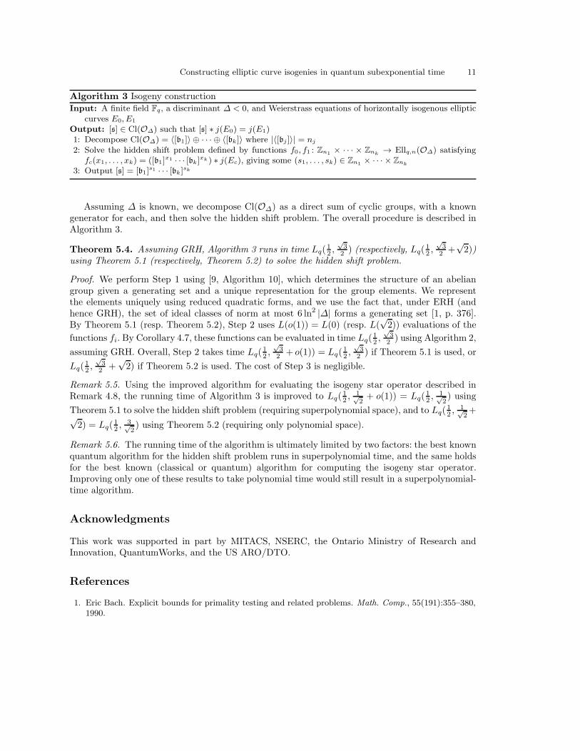
Algorithm 3 Isogeny construction

Input: A finite field Fq, a discriminant ∆ < 0, and Weierstrass equations of horizontally isogenous ellipticcurves E0, E1

Output: [s] ∈ Cl(O∆) such that [s] ∗ j(E0) = j(E1)1: Decompose Cl(O∆) = 〈[b1]〉 ⊕ · · · ⊕ 〈[bk]〉 where |〈[bj ]〉| = nj

2: Solve the hidden shift problem defined by functions f0, f1 : Zn1 × · · · × Znk → Ellq,n(O∆) satisfyingfc(x1, . . . , xk) = ([b1]

x1 · · · [bk]xk ) ∗ j(Ec), giving some (s1, . . . , sk) ∈ Zn1 × · · · × Znk

3: Output [s] = [b1]s1 · · · [bk]sk

Assuming ∆ is known, we decompose Cl(O∆) as a direct sum of cyclic groups, with a knowngenerator for each, and then solve the hidden shift problem. The overall procedure is described inAlgorithm 3.

Theorem 5.4. Assuming GRH, Algorithm 3 runs in time Lq(12 ,

√32 ) (respectively, Lq(

12 ,

√32 +

√2))

using Theorem 5.1 (respectively, Theorem 5.2) to solve the hidden shift problem.

Proof. We perform Step 1 using [9, Algorithm 10], which determines the structure of an abeliangroup given a generating set and a unique representation for the group elements. We representthe elements uniquely using reduced quadratic forms, and we use the fact that, under ERH (andhence GRH), the set of ideal classes of norm at most 6 ln2 |∆| forms a generating set [1, p. 376].By Theorem 5.1 (resp. Theorem 5.2), Step 2 uses L(o(1)) = L(0) (resp. L(

√2)) evaluations of the

functions fi. By Corollary 4.7, these functions can be evaluated in time Lq(12 ,

√32 ) using Algorithm 2,

assuming GRH. Overall, Step 2 takes time Lq(12 ,

√32 + o(1)) = Lq(

12 ,

√32 ) if Theorem 5.1 is used, or

Lq(12 ,

√32 +

√2) if Theorem 5.2 is used. The cost of Step 3 is negligible.

Remark 5.5. Using the improved algorithm for evaluating the isogeny star operator described inRemark 4.8, the running time of Algorithm 3 is improved to Lq(

12 ,

1√2+ o(1)) = Lq(

12 ,

1√2) using

Theorem 5.1 to solve the hidden shift problem (requiring superpolynomial space), and to Lq(12 ,

1√2+√

2) = Lq(12 ,

3√2) using Theorem 5.2 (requiring only polynomial space).

Remark 5.6. The running time of the algorithm is ultimately limited by two factors: the best knownquantum algorithm for the hidden shift problem runs in superpolynomial time, and the same holdsfor the best known (classical or quantum) algorithm for computing the isogeny star operator.Improving only one of these results to take polynomial time would still result in a superpolynomial-time algorithm.

Acknowledgments

This work was supported in part by MITACS, NSERC, the Ontario Ministry of Research andInnovation, QuantumWorks, and the US ARO/DTO.

References

1. Eric Bach. Explicit bounds for primality testing and related problems. Math. Comp., 55(191):355–380,1990.


2. Charles H. Bennett, Ethan Bernstein, Gilles Brassard, and Umesh Vazirani. Strengths and weaknessesof quantum computing. SIAM J. Comput., 26:1510–1523, 1997.

3. Daniel J. Bernstein. How to find smooth parts of integers, 2004. http://cr.yp.to/papers.html#

smoothparts.4. Gaetan Bisson. Computing endomorphism rings of elliptic curves under the GRH. Journal of Mathe-

matical Cryptology (to appear), 2011. arXiv:1101.4323.5. Gaetan Bisson and Andrew V. Sutherland. Computing the endomorphism ring of an ordinary elliptic

curve over a finite field. J. Number Theory, to appear, 2009.6. Alin Bostan, Francois Morain, Bruno Salvy, and Eric Schost. Fast algorithms for computing isogenies

between elliptic curves. Math. Comp., 77(263):1755–1778, 2008.7. Reinier Broker, Denis Charles, and Kristin Lauter. Evaluating large degree isogenies and applications

to pairing based cryptography. In Pairing ’08: Proceedings of the 2nd International Conference onPairing-Based Cryptography, pages 100–112, 2008.

8. Johannes Buchmann and Ulrich Vollmer. Binary quadratic forms: An algorithmic approach, volume 20of Algorithms and Computation in Mathematics. Springer, Berlin, 2007.

9. Kevin K. H. Cheung and Michele Mosca. Decomposing finite abelian groups. Quantum Inform. Com-put., 1(3):26–32, 2001.

10. Jean-Marc Couveignes. Hard homogeneous spaces, 2006. http://eprint.iacr.org/2006/291.11. David A. Cox. Primes of the form x2 + ny2: Fermat, class field theory and complex multiplication.

Wiley, New York, 1989.12. Wim van Dam, Sean Hallgren, and Lawrence Ip. Quantum algorithms for some hidden shift problems.

In SODA ’02: Proceedings of the 14th ACM-SIAM Symposium on Discrete Algorithms, pages 489–498,2002.

13. Mark Ettinger and Peter Høyer. On quantum algorithms for noncommutative hidden subgroups. Ad-vances in Applied Mathematics, 25:239–251, 2000.

14. Luca De Feo. Fast algorithms for computing isogenies between ordinary elliptic curves in small char-acteristic. J. Number Theory, to appear, 2010.

15. M. Fouquet and F. Morain. Isogeny volcanoes and the SEA algorithm. In Algorithmic number theory(Sydney, 2002), volume 2369 of Lecture Notes in Comput. Sci., pages 276–291. Springer, Berlin, 2002.

16. Steven D. Galbraith. Constructing isogenies between elliptic curves over finite fields. LMS J. Comput.Math., 2:118–138 (electronic), 1999.

17. Steven D. Galbraith, Florian Hess, and Nigel P. Smart. Extending the GHS Weil descent attack. InAdvances in Cryptology—EUROCRYPT 2002, volume 2332 of Lecture Notes in Comput. Sci., pages29–44, 2002.

18. Steven D. Galbraith and Anton Stolbunov. Improved algorithm for the isogeny problem for ordinaryelliptic curves, 2011. http://arxiv.org/abs/1105.6331/.

19. Sean Hallgren. Polynomial-time quantum algorithms for Pell’s equation and the principal ideal problem.J. ACM, 54(1):article 4, 2007. Preliminary version in STOC ’02.

20. Jens Hermans, Frederik Vercauteren, and Bart Preneel. Speed records for NTRU. In Josef Pieprzyk,editor, CT-RSA, volume 5985 of Lecture Notes in Computer Science, pages 73–88. Springer, 2010.

21. Sorina Ionica and Antoine Joux. Pairing the volcano. In Algorithmic number theory: Proceedings ofANTS-IX, volume 6197 of Lecture Notes in Comput. Sci., pages 201–218, 2010.

22. David Jao, Stephen D. Miller, and Ramarathnam Venkatesan. Expander graphs based on GRH withan application to elliptic curve cryptography. J. Number Theory, 129(6):1491–1504, 2009.

23. David Jao and Vladimir Soukharev. A subexponential algorithm for evaluating large degree isogenies.In Algorithmic number theory: Proceedings of ANTS-IX, volume 6197 of Lecture Notes in Comput. Sci.,pages 219–233, 2010.

24. Alexei Yu. Kitaev. Quantum measurements and the abelian stabilizer problem. arXiv:quant-ph/9511026.

25. Greg Kuperberg. A subexponential-time quantum algorithm for the dihedral hidden subgroup problem.SIAM J. Comput., 35(1):170–188, 2005.


26. Reynald Lercier and Thomas Sirvent. On Elkies subgroups of l-torsion points in elliptic curves definedover a finite field. J. Theor. Nombres Bordeaux, 20(3):783–797, 2008.

27. Ray A. Perlner and David A. Cooper. Quantum resistant public key cryptography: a survey. InProceedings of the 8th Symposium on Identity and Trust on the Internet, IDtrust ’09, pages 85–93, NewYork, NY, USA, 2009. ACM.

28. Oded Regev. A subexponential time algorithm for the dihedral hidden subgroup problem with polyno-mial space. arXiv:quant-ph/0406151.

29. Alexander Rostovtsev and Anton Stolbunov. Public-key cryptosystem based on isogenies, 2006. http://eprint.iacr.org/2006/145.

30. Arnold Schonhage. Fast reduction and composition of binary quadratic forms. In ISSAC ’91: Pro-ceedings of the 1991 International Symposium on Symbolic and Algebraic Computation, pages 128–133,1991.

31. Rene Schoof. Counting points on elliptic curves over finite fields. J. Theor. Nombres Bordeaux, 7(1):219–254, 1995. Les Dix-huitiemes Journees Arithmetiques (Bordeaux, 1993).

32. Jean-Pierre Serre. Groupes de Lie l-adiques attaches aux courbes elliptiques. In Les Tendances Geom.en Algebre et Theorie des Nombres, pages 239–256. Editions du Centre National de la Recherche Sci-entifique, Paris, 1966.

33. Martin Seysen. A probabilistic factorization algorithm with quadratic forms of negative discriminant.Math. Comp., 48(178):757–780, 1987.

34. Peter W. Shor. Polynomial-time algorithms for prime factorization and discrete logarithms on a quan-tum computer. SIAM J. Comput., 26(5):1484–1509, 1997. Preliminary version in FOCS ’94.

35. Joseph H. Silverman. The arithmetic of elliptic curves, volume 106 of Graduate Texts in Mathematics.Springer-Verlag, New York, 1992. Corrected reprint of the 1986 original.

36. Anton Stolbunov. Constructing public-key cryptographic schemes based on class group action on a setof isogenous elliptic curves. Adv. Math. Commun., 4(2):215–235, 2010.

37. John Tate. Endomorphisms of abelian varieties over finite fields. Invent. Math., 2:134–144, 1966.38. Jacques Velu. Isogenies entre courbes elliptiques. C. R. Acad. Sci. Paris Ser. A-B, 273:A238–A241,

1971.39. William C. Waterhouse. Abelian varieties over finite fields. Ann. Sci. Ecole Norm. Sup. (4), 2:521–560,

1969.

A Subexponential-time and polynomial-space quantum algorithm for

the general abelian hidden shift problem

Following Kuperberg’s discovery of a subexponential-time quantum algorithm for the hidden shiftproblem in any finite abelian group A [25], Regev presented a modification of Kuperberg’s algorithmthat requires only polynomial space, with a slight increase in the running time [28]. However, Regevonly explicitly considered the case A = Z2n , and while he showed that the running time is L|A|(

12 , c),

he did not determine the value of the constant c.In this appendix we describe a polynomial-space quantum algorithm for the general abelian

hidden shift problem using time L|A|(12 ,√2). We use several of the same techniques employed by

Kuperberg [25, Algorithm 5.1 and Theorem 7.1] to go beyond the case A = Z2n , adapted to workwith a Regev-style sieve that only uses polynomial space.

Let A = ZN1× · · · × ZNt be a finite abelian group. Consider the hidden shift problem with

hidden shift s = (s1, . . . , st) ∈ A. By Fourier sampling, one (coherent) evaluation of the hidingfunctions f0, f1 can produce the state

|ψx〉 :=1√2

(

|0〉+ exp

[

2πi

(

s1x1N1

+ · · ·+ stxtNt

)]

|1〉)

(ψ)


with a known value x = (x1, . . . , xt) ∈R A (see for example the proof of Theorem 7.1 in [25]), wherex ∈R A denotes that x occurs uniformly at random from A. For simplicity, we begin by consideringthe case where A = ZN is cyclic. Then Fourier sampling produces states

|ψx〉 =1√2(|0〉+ ωsx|1〉)

where x ∈R ZN is known and ω := e2πi/N .If we could make states |ψx〉 with chosen values of x, then we could determine s. In particular,

the following observation is attributed to Peter Høyer in [25]:

Lemma A.1. Given one copy each of the states |ψ1〉, |ψ2〉, |ψ4〉, . . . , |ψ2k−1〉, where 2k = Ω(N),one can reconstruct s in polynomial time with probability Ω(1).

Proof. We have

k−1⊗

j=0

|ψ2j 〉 =1√2k

2k−1∑

y=0

ωsy|y〉.

Apply the inverse quantum Fourier transform over ZN (which runs in poly(logN) time [24]) and

measure in the computational basis. The Fourier transform of |s〉, namely 1√N

∑N−1y=0 ω

sy|s〉, hasoverlap squared with this state of 2k/N , which implies the claim.

We aim to produce states of the form |ψ2j 〉 using a sieve that combines states to prepare newones with more desirable labels. A basic building block is Algorithm 4, which can be used to producestates with smaller labels.

Lemma A.2. Algorithm 4 runs in time 2k poly(logN) and succeeds with probability Ω(1) provided4k ≤ B/B′ ≤ 2k/k.

Proof. The running time is dominated by the brute force calculation in Step 6 and the projectionin Step 10, both of which can be performed in time 2k poly(logN).

The probability of aborting in Step 2 for any one xi is 1 − 2B′

B ⌊ B2B′

⌋ ≤ 2B′

B , so by the union

bound, the overall probability of aborting in this step is at most k 2B′

B ≤ 1/2. Conditioned on notaborting in Step 2, xi ∈R 0, 1, . . . , 2B′⌊B/2B′⌋ − 1.

Let x · yj = q(2B′) + rj where 0 ≤ rj < 2B′ (q is the measurement outcome, which isindependent of j). By the uniformity of the xis, each rj = x · yj mod 2B′ is uniformly dis-tributed over 0, 1, . . . , 2B′ − 1. Thus the output label is x′ = x · (y ⋆− y⋆) = |r ⋆− r⋆| wherer⋆, r

⋆∈R 0, 1, . . . , 2B′ − 1. A simple calculation shows that the distribution of |r ⋆− r⋆| is

Pr(|r ⋆− r⋆| = ∆) =

12B′

for ∆ = 02B′−∆2B′2 for ∆ ∈ 1, . . . , 2B′ − 1.

Thus the probability that we abort in Steps 12–16 is 1/2, and conditioned on not aborting in thesesteps, x′ ∈R 0, 1, . . . , B′ − 1. Thus the algorithm is correct if it reaches Step 17.

It remains to show that the algorithm succeeds with constant probability. We have alreadybounded the probability that we abort in Step 2 and Steps 12–16. Since y = 0 occurs with probability


Algorithm 4 Combining states to give smaller labels

Input: Parameters B,B′ and states |ψx1〉, . . . , |ψxk 〉 with known x1, . . . , xk ∈R 0, 1, . . . , B − 1Output: State |ψx′〉 with known x′ ∈R 0, 1, . . . , B′ − 11: if ∃i : xi ≥ 2B′⌊B/2B′⌋ then2: Abort3: end if

4: Introduce an ancilla register and compute

1√2k

∑

y∈0,1k

ωs(x·y)|y〉|⌊(x · y)/2B′⌋〉

where x · y :=∑k

i=1 xiyi5: Measure the ancilla register, giving an outcome q and a state

1√ν

ν∑

j=1

ωs(x·yj)|yj〉

where y1, . . . , yν 6= 0k are the k-bit strings such that ⌊(x · yj)/2B′⌋ = q6: Compute y1, . . . , yν by brute force7: if ν = 1 then

8: Abort9: end if

10: Project onto span|y1〉, |y2〉 or span|y3〉, |y4〉 or . . . or span|y2⌊ν/2⌋−1〉, |y2⌊ν/2⌋〉, giving an outcomespan|y⋆〉, |y ⋆〉

11: Let x′ = x · (y ⋆− y⋆) where x · y ⋆≥ x · y⋆ WLOG12: if x′ ∈ 1, . . . , B′ − 1 then13: Abort with probability B′/(2B′ − x′)14: else if x′ ∈ B′, . . . , 2B′ − 1 then15: Abort16: end if

17: Relabel |y⋆〉 7→ |0〉 and |y ⋆〉 7→ |1〉, giving a state |ψx′〉

2−k and at most one state |yν〉 can be unpaired (and this only happens when ν is odd), the projectionin Step 10 fails with probability at most ν−1 + 2−k ≤ 1/3 + o(1). We claim that the probabilityof aborting in Step 8 (i.e., the probability that ν = 1) is also bounded away from 1. Call a valueof q bad if ν = 1. Since 0 ≤ x · y ≤ k(B − 1), there are at most kB/2B′ possible values of q, andin particular, there can be at most kB/2B′ bad values of q. Since the probability of any particularbad q is 1/2k, the probability that q is bad is at most kB/B′2k+1 ≤ 1/2. This completes the proof.

We apply this combination procedure using the generalized sieve of Algorithm 5, which is equiv-alent to Regev’s “pipeline of routines” [28].

Lemma A.3. Suppose me−2k = o(1). Then Algorithm 5 is correct, succeeds with probability 1−o(1)using k(1+o(1))m state preparations and combination operations, and uses space O(mk).

Proof. If Algorithm 5 outputs a state from Sm then it is correct. Since the algorithm never storesmore than O(mk) states at a time, it uses space O(mk). It remains to show that the algorithm islikely to succeed using only k(1+o(1))m state preparations and combination operations.


Algorithm 5 Sieving quantum states

Input: Procedures to prepare states from a set S0 and to combine k states from Si−1 to make a state fromSi with probability at least p for each i ∈ 1, . . . , m

Output: State from Sm

1: repeat

2: while for all i we have fewer than k states from Si do

3: Make a state from S0

4: end while

5: Combine k states from some Si to make a state from Si+1 with probability at least p6: until there is a state from Sm

If we could perform combinations deterministically, we would need

1 state from Sm,

k states from Sm−1,

k2 states from Sm−2,

...

km states from S0.

Since the combinations only succeed with probability p, we lower bound the probability of eventuallyproducing (2k/p)m−i states from Si for each i ∈ 1, . . . ,m (so in particular, we produce one statefrom Sm). Given (2k/p)m−i+1 states from Si−1, the expected number of successful combinationsis p(2k/p)m−i+1/k = 2(2k/p)m−i, whereas only (2k/p)m−i successful combinations are needed. Bythe Chernoff bound, the probability of having fewer than (2k/p)m−i successful combinations is at

most e−p(2k/p)m−i

. Thus, by the union bound, the probability that the algorithm fails is at most

m−1∑

i=1

e−p(2k/p)m−i ≤ me−2k,

so the probability of success is 1− o(1).Finally, the number of states from S0 is (2k/p)m = k(1+o(1))m and the total number of combi-

nations is∑m−1

i=0 (2k/p)m−i/k = k(1+o(1))m.

When using the sieve, we have the freedom to choose the relationship between k and m tooptimize the running time. Suppose that mk = (1 + o(1)) log2N (intuitively, to cancel log2N bitsof the label), and also suppose that the combination operation takes time 2k poly(logN) (as inLemma A.2). Then if we take k = c

√

log2N log2 log2N , we find that the overall running time

of Algorithm 5 is 2k2(1+o(1))m log2 k poly(logN) = LN (12 , c +12c ). Choosing c = 1√

2gives the best

running time, LN (12 ,√2).

We now consider how to apply the sieve. To use Lemma A.1, our goal is to prepare states of theform |ψ2j 〉 for each j ∈ 0, 1, . . . , ⌊log2N⌋. First we show how to prepare the state |ψ1〉 in timeLN(12 ,

√2) using Algorithm 4 as the combination procedure in Algorithm 5. For i ∈ 0, 1, . . . ,m,

the ith stage of the sieve produces states with labels from Si = 0, 1, . . . , Bi − 1. Lemma A.4below shows that there is a choice of the Bi with B0 = N , Bm = 2, and successive ratios of the


Bis satisfying the conditions of Lemma A.2, such that 2kk(1+o(1))m = LN (12 ,√2). It then follows

that Algorithm 5 produces a uniformly random label from Sm = 0, 1 with constant probabilityin time LN(12 ,

√2), and in particular, can be used to produce a copy of |ψ1〉 in time LN (12 ,

√2).

Lemma A.4. There is a constant N0 such that for all N > N0, letting Bi = ⌊N/ρi⌋ where ρ =(N/2)1/m and

k =

⌊

√

12 log2N log2 log2N

⌋

m =

⌈

log2N/2

k − log2 2k

⌉

= Θ

(√

log2N

log2 log2N

)

,

we have B0 = N , Bm = 2, and 4k ≤ Bi−1/Bi ≤ 2k/k for all i ∈ 1, . . . ,m.

Proof. Clearly B0 = N , and the value of ρ is chosen so that Bm = 2.For i ∈ 1, . . . ,m, we have

Bi−1

Bi=

⌊N/ρi−1⌋⌊N/ρi⌋ ≤ N/ρi−1

N/ρi − 1=

ρ

1− ρi/N.

Since ρi/N ≤ ρm/N = 1/2, we have Bi−1/Bi ≤ 2ρ. Then using

ρ ≤ (N/2)k−log2 2k

log2 N/2 =2k

2k

gives Bi−1/Bi ≤ 2k/k as claimed.Similarly, we have

Bi−1

Bi=

⌊N/ρi−1⌋⌊N/ρi⌋ ≥ N/ρi−1 − 1

N/ρi= ρ− ρi/N ≥ ρ− 1

2 .

Since

ρ = (N/2)Θ(√

log2 log2 N/ log2 N) = 2Θ(√

log2 N log2 log2 N) = 2Θ(k),

we have ρ− 12 ≥ 4k for sufficiently large N . This completes the proof.

If N is odd, then division by 2 is an automorphism of ZN . Thus we can prepare |ψ2j 〉 byperforming the above sieve under the automorphism x 7→ 2−jx. It follows that the abelian hiddenshift problem in a cyclic group of odd order N can be solved in time LN(12 ,

√2).

Now suppose that N = 2n is a power of 2. In this case, we first use a combination procedurethat zeros out low-order bits, as described in Algorithm 6. We use the notation xS := xz : z ∈ Sfor any x ∈ Z and S ⊂ Z.

Lemma A.5. Algorithm 6 runs in time 2k poly(logN) and succeeds with probability Ω(1) providedk ≥ ℓ′ − ℓ+ 1.

Proof. The proof is similar to that of Lemma A.2. Again the running time is dominated by thebrute force calculation in Step 3 and the projection in Step 7, both of which can be performed intime 2k poly(logN).


Algorithm 6 Combining states to cancel low-order bits

Input: Parameters ℓ, ℓ′ and states |ψx1〉, . . . , |ψxk〉 with known x1, . . . , xk ∈R 2ℓ0, 1, . . . , N/2ℓ − 1Output: State |ψx′〉 with known x′ ∈R 2ℓ

′0, 1, . . . , N/2ℓ′ − 11: Introduce an ancilla register and compute

1√2k

∑

y∈0,1k

ωs(x·y)|y〉|x · y mod 2ℓ′〉

2: Measure the ancilla register, giving an outcome r and a state

1√ν

ν∑

j=1

ωs(x·yj)|yj〉

where y1, . . . , yν 6= 0k are the k-bit strings such that x · yj mod 2ℓ′

= r3: Compute y1, . . . , yν by brute force4: if ν = 1 then

5: Abort6: end if


8: Relabel |y⋆〉 7→ |0〉 and |y ⋆〉 7→ |1〉, giving a state |ψx′〉 with x′ = x · (y ⋆− y⋆) mod N

We claim that the algorithm is correct if it reaches Step 8. Observe that x ·yj mod N = qj2ℓ′

+rwhere r is independent of j. Since yj 6= 0k, x · yj mod N ∈R 2ℓ0, 1, . . . , N/2ℓ − 1, so qj ∈R

0, 1, . . . , N/2ℓ′ − 1, and hence x′ = (q⋆− q⋆)2ℓ

′

mod N ∈R 2ℓ′0, 1, . . . , N/2ℓ′ − 1 as required.

The projection in Step 7 fails with probability at most 1/3 + o(1). It remains to show that thealgorithm reaches Step 7 with probability Ω(1), i.e., to upper bound the probability that ν = 1.Call a value of r bad if ν = 1. There are 2ℓ

′−ℓ possible values of r, so in particular there are at most2ℓ

′−ℓ bad values of r. Since the probability of any particular bad r is 1/2k, the probability that ris bad is at most 2ℓ

′−ℓ−k ≤ 1/2. This completes the proof.

Algorithm 6 is similar to the combination procedure used in [28], but differs in that the latterrequires ν = O(1), which is established in the analysis using a second moment argument. Themodification of pairing as many values of y as possible allows us to use a simpler analysis (withessentially the same performance).

To produce a state of the form |ψ2j 〉, we first use Algorithm 6 to cancel low-order bits and thenuse Algorithm 4 to cancel high-order bits. Note that if all states |ψx〉 have labels x with a commonfactor—say, 2j |x—then we can view the labels as elements of Z2n−j and apply Algorithm 4 to affectthe n − j most significant bits. Specifically, to make the state |ψ2j 〉, we apply Algorithm 5 usingAlgorithm 6 as the combination procedure that produces states from Si using states from Si−1

for i ∈ 1, . . . ,m1 + 1, and Algorithm 4 (on the n − j most significant bits) as the combinationprocedure for i ∈ m1 + 2, . . . ,m1 +m2 + 1, taking

Si =

2(k−1)i0, 1, . . . , 2n−(k−1)i − 1 for i ∈ 0, 1, . . . ,m12j0, 1, . . . , Bi − 1 for i ∈ m1 + 1, . . . ,m1 +m2 + 1


where now

Bi = ⌊2n−j/ρi−m1−1⌋ m1 = ⌊j/(k − 1)⌋

ρ = 2(n−j−1)/m2 m2 =

⌈

n− j

k − log2 2k

⌉

and again k = ⌊√

12 log2N log2 log2N⌋. When making states in Si from states in Si−1 for i ∈

1, . . . ,m1, we cancel k − 1 bits with k states, so the condition of Lemma A.5 is satisfied. Fori = m1+1, we cancel j− (k−1)m1 = j− (k−1)⌊j/(k − 1)⌋ ≤ j− (k−1)[j/(k−1)−1] = k−1 bits,so again the condition of Lemma A.5 is satisfied. For i ∈ m1 + 2, . . . ,m1 +m2 + 1, Lemma A.4implies that the conditions of Lemma A.2 are satisfied provided 2n−j ≥ N0. (If 2

n−j < N0 then weonly need to perform the firstm1+1 stages of the sieve, producing a state uniformly at random fromSm1+1; in this case |Sm1+1| = O(1), so O(1) repetitions suffice to produce a copy of |ψ2j 〉.) Finally,since (m1 +m2 + 1)k = (1 + o(1))n, the discussion following Lemma A.3 shows that Algorithm 5takes time LN(12 ,

√2).

So far we have covered the case where the group is A = ZN with N either odd or a power of2. Now consider the case of a general finite abelian group A = ZN1

× · · · × ZNt . By the Chineseremainder theorem, we can assume without loss of generality that each Ni is either odd or a powerof 2. Consider what happens if we apply Algorithm 4 or Algorithm 6 to one component of a productof cyclic groups. Suppose we combine k states of the form of Eqn. (ψ). For each i ∈ 1, . . . , k, letxi ∈ ZN1

×· · ·×ZNt denote the label of the ith state, with xi,j ∈ ZNj for j ∈ 1, . . . , t. To addressthe ℓth component of A, the combination procedure prepares a state

1√2k

∑

y∈0,1k

exp

2πik∑

i=1

t∑

j=1

yixi,jsjNj

|y〉|h(∑ki=1 xi,ℓyi)〉

for some function h (a quotient in Algorithm 4 or a remainder in Algorithm 6). For j 6= ℓ, if xi,j = 0

for all i ∈ 1, . . . , k then x′j =∑k

i=1 xi,j(y

⋆

i − y⋆i ) = 0, so components that are initially zero remainzero. Thus, if we can prepare states |ψx〉 with xℓ ∈R ZNℓ

(for any desired ℓ ∈ 1, . . . , t) and allother components zero, we effectively reduce the problem to the cyclic case.

To prepare such states, we use a new combination procedure, Algorithm 7. Without loss ofgenerality, our goal is to zero out the first t− 1 components, leaving the last one uniformly randomfrom ZNt . Algorithm 7 is similar to Algorithm 4, viewing the first t − 1 components of the labelxi ∈ ZN1

× · · · × ZNt as the mixed-radix integer

µ(xi) :=t−1∑

j=1

xi,j

j−1∏

j′=1

Nj′ .

Because we are merely trying to zero out certain components, we no longer require uniformity ofthe states output by the sieve, which simplifies the procedure and its analysis.

Lemma A.6. Algorithm 7 runs in time 2k poly(logN) and succeeds with probability Ω(1) providedB/B′ ≤ 2k/2k.

Proof. As in Lemma A.2 and Lemma A.5, the running time is dominated by the brute force calcula-tion in Step 3 and the projection in Step 7, both of which can be performed in time 2k poly(logN).


Algorithm 7 Combining non-cyclic states to reduce undesired components

Input: Parameters B,B′ and states |ψx1〉, . . . , |ψxk 〉 with known x1, . . . , xk ∈ ZN1 × · · · × ZNt satisfyingµ(xi) ∈ 0, 1, . . . , B − 1 for each i ∈ 1, . . . , k, with xi,t ∈R ZNt

Output: State |ψx′〉 with known x′ ∈ ZN1 ×· · ·×ZNt satisfying µ(x′) ∈ 0, 1, . . . , B′−1, with x′t ∈R ZNt

1: Introduce an ancilla register and compute

1√2k

∑

y∈0,1k

exp

(

2πi

k∑

i=1

t∑

j=1

yixi,jsjNj

)

|y〉|⌊∑ki=1 µ(xi)yi/B

′⌋〉

2: Measure the ancilla register, giving an outcome q and a state

1√ν

ν∑

j=1

exp

(

2πi

k∑

i=1

t∑

j=1

yixi,jsjNj

)

|yj〉

where y1, . . . , yν 6= 0k are the k-bit strings such that ⌊∑ki=1 µ(xi)y

ji /B

′⌋ = q3: Compute y1, . . . , yν by brute force4: if ν = 1 then

5: Abort6: end if


8: Relabel |y⋆〉 7→ |0〉 and |y ⋆〉 7→ |1〉 where ∑ki=1 µ(xi)y

⋆

i ≥∑k

i=1 µ(xi)y⋆i WLOG, giving a state |ψx′〉

with x′j =

∑ki=1 xi,j(y

⋆

i − y⋆i ) for each j ∈ 1, . . . , t

We claim that the algorithm is correct if it reaches Step 8. Since∑k

i=1 µ(xi)yji = qB′+ rj where

q is independent of j and 0 ≤ rj < B′, we have

µ(x′) =t−1∑

j=1

x′j

j−1∏

j′=1

Nj′ =

t−1∑

j=1

k∑

i=1

xi,j(y

⋆

i − y⋆i )

j−1∏

j′=1

Nj′ =

k∑

i=1

µ(xi)(y

⋆

i − y⋆i ) = r

⋆− r⋆ < B′

as required. Since y⋆ 6= y

⋆

and the xi,t are uniformly random, x′t =∑k

i=1 xi,t(y

⋆

i − y⋆i ) is uniformlyrandom as required.

The projection in Step 7 fails with probability at most 1/3 + o(1). We claim the algorithmreaches Step 7 with probability Ω(1). To show this, we need to upper bound the probability that

ν = 1. Call a value of q bad if ν = 1. Since 0 ≤∑ki=1 µ(xi)yi ≤ k(B − 1), there are at most kB/B′

possible values of q, and in particular, there can be at most kB/B′ bad values of q. Since theprobability of any particular bad q is 1/2k, the probability that q is bad is at most kB/B′2k ≤ 1/2.This completes the proof.

To apply Algorithm 7 as the combination procedure for Algorithm 5, we require a straightforwardvariant of Lemma A.4, as follows.

Lemma A.7. There is a constant N ′0 such that for all N > N ′

0, letting Bi = ⌊N/ρi⌋ where ρ =N1/m and

k =

⌊

√

12 log2N log2 log2N

⌋

m =

⌈

log2N

k − log2 4k

⌉

= Θ

(√

log2N

log2 log2N

)

,


Algorithm 8 Abelian hidden shift problem

Input: Black box for the hidden shift problem in an abelian group AOutput: Hidden shift s1: Write A = ZN1 × · · · × ZNt where each Ni is either odd or a power of 22: for all i ∈ 1, . . . , t do3: if Ni is odd then

4: for all j ∈ 0, . . . , ⌊log2Ni⌋ do5: Apply Algorithm 5, first using Algorithm 7 to zero out all components except the ith one

and then using Algorithm 4 under the ZNi -automorphism x 7→ 2−jx to produce a copy of|ψ(0,...,0,2j ,0,...,0)〉 (see the proof of Theorem A.1 for detailed parameters)

6: end for

7: else

8: Let Ni = 2n

9: for all j ∈ 0, . . . , n− 1 do10: Apply Algorithm 5, first using Algorithm 7 to zero out all components except the ith one, then

using Algorithm 6 to make states |ψ(0,...,0,x,0,...,0)〉 with 2j |x, and finally using Algorithm 4 toproduce a copy of |ψ(0,...,0,2j ,0,...,0)〉 (see the proof of Theorem A.1 for detailed parameters)

11: end for

12: end if

13: Apply Lemma A.1 with N = Ni to give si14: end for

15: Output s = (s1, . . . , st)

we have B0 = N , Bm = 1, and Bi−1/Bi ≤ 2k/2k for all i ∈ 1, . . . ,m.

Proof. Clearly B0 = N , and the value of ρ is chosen so that Bm = 1.

We have Bm−1 ≤ N/ρm−1 = ρ, and since

ρ ≤ Nk−log2 4k

log2 N =2k

4k,

the claimed inequality holds for i = m.

For i ∈ 1, . . . ,m− 1,

Bi−1

Bi=

⌊N/ρi−1⌋⌊N/ρi⌋ ≤ N/ρi−1

N/ρi − 1=

ρ

1− ρi/N.

Since ρi/N ≤ ρm−1/N = 1/ρ, we have Bi−1/Bi ≤ ρ/(1− 1/ρ). Then using

ρ = NΘ(√

log2 log2 N/ log2 N) = 2Θ(√

log2 N log2 log2 N),

we have ρ ≥ 2 provided N > N ′0 for some constant N ′

0, which implies Bi−1/Bi ≤ 2k/2k. Thiscompletes the proof.

Combining these ideas, the overall procedure is presented in Algorithm 8.

Theorem A.1. Algorithm 8 runs in time L|A|(12 ,√2).


Proof. In Step 1, if the structure of the group is not initially known, it can be determined inpolynomial time using [9]. Given the structure of the group, for each term ZN we can easily factorN = 2nM where M is odd; then ZN

∼= Z2n × ZM , and we obtain a decomposition of the desiredform.

Now suppose without loss of generality that we are trying to determine st (i.e., i = t in Step 2).The main contribution to the running time comes from the sieves in Step 5 (for Nt odd) and Step 10(for Nt a power of 2).

First suppose that Nt is odd. It suffices to handle the case where j = 0, so we are making thestate |ψ(0,...,0,1)〉. Then we apply Algorithm 5 with

Si =

x ∈ A : µ(x) < Bi for i ∈ 0, 1, . . . ,m1x ∈ A : µ(x) = 0 and xt < Bi for i ∈ m1 + 1, . . . ,m2

where

Bi =

⌊(N/Nt)/ρi1⌋ for i ∈ 0, 1, . . . ,m1

⌊Nt/ρi−m1

2 ⌋ for i ∈ m1 + 1, . . . ,m1 +m2

with

ρ1 = (N/Nt)1/m1 m1 =

⌈

log2N/Nt

k − log2 4k

⌉

ρ2 = (Nt/2)1/m2 m2 =

⌈

log2Nt/2

k − log2 2k

⌉

and k = ⌊√

12 log2N log2 log2N⌋. We use Algorithm 7 as the combination procedure for the firstm1

stages of Algorithm 5. By Lemma A.7, the condition of Lemma A.6 is satisfied providedN/Nt > N ′0;

otherwise we can produce a state with a label from Sm1in only O(1) trials. Then we proceed to

apply Algorithm 4 as the combination procedure for the remaining m2 stages of Algorithm 5. ByLemma A.4, the conditions of Lemma A.2 are satisfied provided Nt > N0; otherwise, producingstates with labels from Sm1

already suffices to produce the desired state with constant probability.Since (m1 +m2)k = (1 + o(1)) log2N , Step 5 takes time L|A|(

12 ,√2) (see the discussion following

the proof of Lemma A.3).

Now suppose that Nt = 2n is a power of 2. Then we apply Algorithm 5 with

Si =

x ∈ A : µ(x) < Bi for i ∈ 0, 1, . . . ,m1

x ∈ A : µ(x) = 0 and xt ∈ 2(k−1)i0, 1, . . . , 2n−(k−1)i

for i ∈ m1 + 1, . . . ,m1 +m2

x ∈ A : µ(x) = 0 and xt ∈ 2j0, 1, . . . , Bi − 1 for i ∈ m1 +m2 + 1, . . . ,

m1 +m2 +m3 + 1

where

Bi =

⌊(N/Nt)/ρi1⌋ for i ∈ 0, 1, . . . ,m1

⌊2n−j/ρi−m1−m2−13 ⌋ for i ∈ m1 +m2 + 1, . . . ,m1 +m2 +m3 + 1


with

ρ1 = (N/Nt)1/m1 m1 =

⌈

log2N/Nt

k − log2 4k

⌉

m2 = ⌊j/(k − 1)⌋

ρ3 = 2(n−j−1)/m3 m3 =

⌈

n− j − 1

k − log2 2k

⌉

and again k = ⌊√

12 log2N log2 log2N⌋. We use Algorithm 7 as the combination procedure for the

firstm1 stages, Algorithm 6 for the nextm2+1 stages, and Algorithm 4 (on the n−j most significantbits) for the final m3 stages. By Lemma A.7 and Lemma A.4, the conditions of Lemma A.6 andLemma A.2 are satisfied, respectively. Since we cancel at most k − 1 bits in each stage that usesAlgorithm 6, the conditions of Lemma A.5 are satisfied for the intermediate stages. Finally, since(m1 +m2 +m3 + 1)k = (1 + o(1)) log2N , Step 10 takes time L|A|(

12 ,√2).

The loops in Step 2, Step 4, and Step 9 only introduce polynomial overhead. Step 13 takespolynomial time and Step 15 is negligible. Thus the overall running time is L|A|(

12 ,√2) as claimed.

constructingelliptic curveisogenies in quantum ... · constructingelliptic curveisogenies in...

Documents