construction of probability distributions in high

HAL Id: hal-00684517https://hal-upec-upem.archives-ouvertes.fr/hal-00684517

Submitted on 2 Apr 2012

HAL is a multi-disciplinary open accessarchive for the deposit and dissemination of sci-entific research documents, whether they are pub-lished or not. The documents may come fromteaching and research institutions in France orabroad, or from public or private research centers.

L’archive ouverte pluridisciplinaire HAL, estdestinée au dépôt et à la diffusion de documentsscientifiques de niveau recherche, publiés ou non,émanant des établissements d’enseignement et derecherche français ou étrangers, des laboratoirespublics ou privés.

Construction of probability distributions in highdimension using the maximum entropy principle:

Applications to stochastic processes, random fields andrandom matrices

Christian Soize

To cite this version:Christian Soize. Construction of probability distributions in high dimension using the maximumentropy principle: Applications to stochastic processes, random fields and random matrices. In-ternational Journal for Numerical Methods in Engineering, Wiley, 2008, 76 (10), pp.1583-1611.�10.1002/nme.2385�. �hal-00684517�

https://hal-upec-upem.archives-ouvertes.fr/hal-00684517

https://hal.archives-ouvertes.fr

INTERNATIONAL JOURNAL FOR NUMERICAL METHODS IN ENGINEERINGInt. J. Numer. Meth. Engng 2008; 0:1–29 Prepared using nmeauth.cls [Version: 2002/09/18 v2.02]

Construction of probability distributions in high dimension usingthe maximum entropy principle. Applications to stochastic

processes, random fields and random matrices

Christian Soize1

1Universite Paris-Est, Laboratoire Modelisation et Simulation Multi Echelle, MSME FRE3160 CNRS, 5 BdDescartes, 77454 Marne la Vallee, France

SUMMARY

The construction of probabilistic models in computational mechanics requires the effective constructionof probability distributions of random variables in high dimension. This paper deals with the effectiveconstruction of the probability distribution in high dimension of a vector-valued random variable usingthe maximum entropy principle. The integrals in high dimension are then calculated in constructing thestationary solution of an Ito stochastic differential equation associated with its invariant measure. Arandom generator of independent realizations is explicitly constructed in the paper. Three fundamentalapplications are presented. The first one is a new formulation of the stochastic inverse problem relativeto the construction of the probability distribution in high dimension of an unknown non-stationaryrandom time series (random accelerograms) for which the Velocity Response Spectrum is given. Thesecond one is also a new formulation related to the construction of the probability distribution ofpositive-definite band random matrices. Finally, we present an extension of the theory when thesupport of the probability distribution is not all the space but is any part of the space. The thirdapplication is then a new formulation related to the construction of the probability distribution of theKarhunen-Loeve expansion of Non-Gaussian positive-valued random fields. Copyright c© 2008 JohnWiley & Sons, Ltd.

key words: Maximum entropy principle; High dimension; Stochastic process; Random matrix,

Karhunen-Loeve expansion, Random fields

1. Introduction

The probabilistic modeling of uncertainties in computational sciences such as in computationalmechanics is a great challenge. For instance, the parametric probabilistic approach whichallows data uncertainties to be taken into account consists in modeling uncertain parametersof the computational model by random variables, stochastic processes and random fields. Suchapproaches have extensively been developed in the two last decades [1, 2]. In particular, the use

∗Correspondence to: Christian Soize, Universite Paris-Est, Laboratoire Modelisation et Simulation MultiEchelle, MSME FRE3160 CNRS, 5 Bd Descartes, 77454 Marne la Vallee, France

Received May 2007Copyright c© 2008 John Wiley & Sons, Ltd. Revised February 2008

Accepted

2 C. SOIZE

of the Gaussian Chaos representation for stochastic processes and random fields [3] has beenused to introduce and to develop useful and very efficient tools for analyzing stochastic systemsusing stochastic finite elements (see [4, 5, 6]). More recently, additional developments have beenproposed to construct Chaos representations with arbitrary probability measures [7]. Modeluncertainties introduced by the mathematical-mechanical process used during the constructionof the computational model of complex systems are much more difficult to take into accountbecause the parametric probabilistic approach cannot address such model uncertainties. Inthis context, a nonparametric probabilistic approach of model uncertainties has recently beenproposed as a possible way to circumvent these difficulties [8, 9, 10] and is based on the use ofthe random matrix theory.In general, the response of a computational model is a nonlinear mapping of the uncertainparameters and consequently, a complete probability model of these uncertain parameters hasto be constructed. This means that the probability distributions of the random quantities ofinterest such as vector-valued random variables, random matrices, etc, have to be constructedand random generators of independent realizations have to be derived from the knowledge ofthe probability distributions. It is well known that the Maximum Entropy (MaxEnt) Principle[11, 12] is certainly one of the most efficient method allowing an explicit construction of suchprobability distributions to be performed using only the available information. This powerfulmethod developed by Shannon in the context of the Information Theory is extremely usefulin many situations for which statistical data related to the random variable of interest areeither partially available or not available at all. We are then considering the case for which thenumber of independent realizations (which constitute the available statistical data obtainedfrom measurements) is too small to obtain a good convergence of the statistical estimatorof the probability density function using nonparametric statistics [13]. The MaxEnt principlehas been used for different cases and in many applications (see for instance: [14] for a simpleoverview concerning the MaxEnt Principle with applications, [15] for advanced developmentsin Physics, [16] for the use of the MaxEnt principle in stochastic dynamics). It should be notedthat this paper does not deal with the maximum entropy in the moment problem [17, 18, 19, 20]but is devoted to general nonlinear constraints in high dimension which are not polynomials,that is to say, which are not expressed as a linear combination of moments.Let us consider a �

N -valued random variable A = (A1, . . . , AN ) in which N is large (highdimension). For instance, the set {A1, . . . , AN} can represent a random time series constructedfrom the time sampling �(t1), . . . ,�(tN ) of a stochastic process {�(t), t ∈ T }. Random vector Acan also be used to generate a sparse random matrix [G] whose non zero random elements areexpressed in function of A. Finally, A can be the vector constituted of the random coordinatesin the Karhunen-Loeve expansion of a random field. The use of the MaxEnt principle allowsthe probability density function a �→ pA(a) on �

N (with respect to the Lebesgue measureda) of random variable A to be constructed using the available information. Introducing theLagrange multiplier � ∈ Lμ ⊂ �

μ associated with the constraints defined by the availableinformation, in which Lμ is the subset of �μ of all the admissible values of �, it can be proventhat pA depends on �. Lagrange multiplier � is then calculated solving a nonlinear algebraicequation or equivalently, solving an optimization problem for a convex cost function. Foreach given value of � in Lμ ⊂ �

μ, an integral iN (�) on �N must be computed. In high

dimension, such a calculation is very difficult to perform and in general, induces a highnumerical cost. Thus there are two main problems. The first one is related to the effectivecalculation of Lagrange multiplier � using an adated algorithm which requires the evaluation

Copyright c© 2008 John Wiley & Sons, Ltd. Int. J. Numer. Meth. Engng 2008; :1–29Prepared using nmeauth.cls

CONSTRUCTION OF PROBABILITY DISTRIBUTIONS IN HIGH DIMENSION 3

of a large number of integral iN (�) in high dimension. The second one is to construct a randomgenerator of independent realizations of random variable A whose pA has been constructedwith the MaxEnt principle. It should be noted that these two problems are not trivial in highdimension. In this paper, we propose a method to solve these two main problems. Integral iN (�)is calculated in constructing the stationary solution associated with the invariant measure ofa nonlinear Ito stochastic differential equation (ISDE) depending on �. This proposed methodis an alternative to the Metropolis-Hastings algorithm or to the Gibbs sampling (see Section4). Such a nonlinear ISDE is solved by using either an explicit Euler scheme or a semi-implicitscheme. Integral iN (�) is then calculated using (1) either the ergodic method or (2) the MonteCarlo method with the usual estimator of the mathematical expectation with ns independentrealizations constructed with a generator. This generator of independent realizations of A isthen constructed solving ns times the ISDE with ns independent Wiener stochastic processes.Three fundamental applications are presented. The first one is a new formulation of thestochastic inverse problem relative to the construction of the probability distribution in highdimension and of its generator for a vector-valued random variable corresponding to anunknown non-stationary random time series (random accelerograms) for which the VelocityResponse Spectrum is given (see Section 7). The second one is also a new formulation relatedto the construction of the probability distribution in high dimension and of its generator forpositive-definite band random matrices (see Section 8). Finally, we present an extension of thetheory corresponding to the case for which the support of the probability distribution in highdimension of random variable A is not �N but is any part A of �N (see Section 9). The thirdapplication is then a new formulation related to the construction of the probability distributionin high dimension for the Karhunen-Loeve expansion of Non-Gaussian positive-valued randomfields.

2. Construction of probability distributions using the maximum entropy principle

Let a = (a1, . . . , aN ) be any vector in �N . Let A = (A1, . . . , AN ) be a �

N -valued second-order random variable for which the probability distribution PA(da) on �

N is unknown butis represented by a probability density function a �→ pA(a) from �

N into �+ = [0 , +∞[

with respect to the Lebesgue measure da = da1 . . . daN and which has to verify the followingnormalization condition, ∫

�N

pA(a) da = 1 . (1)

Presently, it is assumed that the support of the probability density function pA is �N . Thecase for which the support of pA is any part A of �N will be treated in Section 9.

The problem to be solved is the construction of the unknown probability density functionpA by using the MaxEnt principle for which the constraints associated with the availableinformation are assumed to be defined by the following equation on �

μ,

E{g(A)} = f , (2)

in which f = (f1, . . . , fμ) is a given vector in �μ with μ ≥ 1, where a �→ g(a) =

(g1(a), . . . , gμ(a)) is a given measurable mapping from �N into �

μ and where E is the


4 C. SOIZE

mathematical expectation. Equation (2) can then be rewritten as∫�N

g(a) pA(a) da = f . (3)

Let C be the set of all the probability density functions a �→ pA(a) defined on �N with values

in �+ such that Eqs. (1) and (3) hold. The maximum entropy principle [11, 12] consists in

constructing pA ∈ C such thatpA = argmax

p∈CS(p) , (4)

in which the entropy S(p) of probability density function p is defined by

S(p) = −∫�N

p(a) log(p(a)) da , (5)

where log is the Neperian logarithm. In order to solve the optimization problem defined byEq. (4), a Lagrange multiplier λ0 ∈ �

+ associated with the constraint defined by Eq. (1) anda Lagrange multiplier � ∈ Lμ ⊂ �

μ associated with the constraint defined by Eq. (3) areintroduced, in which Lμ is the subset of �μ of all the admissible values of �. It can then beproven that the solution of Eq. (4) can be written as

pA(a) = csol0 exp(− < �sol, g(a) >μ) , ∀a ∈ �

N , (6)

with csol0 = exp(−λsol

0 ) in which (λsol0 ,�sol) ∈ �

+×Lμ is such that Eqs. (1) and (3)) are verified.In Eq. (6), < x , y >μ= x1y1 + . . . + xμyμ is the Euclidean inner product on �

μ.For � fixed in Lμ, let B� be the �

N -valued random variable whose probability densityfunction b �→ p(b,�) from �

N into �+ (with respect to the Lebesgue measure db on �

N ) iswritten as

p(b,�) = c� exp(− < �, g(b) >μ) , ∀b ∈ �N , (7)

in which c� is a finite positive constant depending on � defined by the following normalizationcondition ∫

�N

p(b,�) db = 1 . (8)

Taking c�sol = csol0 , Eqs. (6) and (7) yield

pA(a) = p(a,�sol) , ∀ a ∈ �N , . (9)

which means that we have the following equality A = B�sol of random variables for theconvergence in probability distribution. From Eqs. (3), (6), (7) and (9), it can then be deducedthat �sol is a solution of the following equation in �,

E{g(B�)} = f , (10)

in which the integral E{g(B�)} which depends on � is such that

E{g(B�)} =∫�N

g(b) p(b,�) db . (11)

We must then construct a solution �sol in Lμ ⊂ �μ of Eq. (10) in �. By construction, the

constraints associated with the available information (see Eq. (3)) are such that the algebraic



equation in � (defined by Eq. (10)) admits a unique solution in Lμ ⊂ �μ (it should be noted

that, if it was not the case, it would mean that the available information defined was notconsistent and consequently, should be re-examined and then modified). We will denote anyone of this by �sol ∈ �

μ. Consequently, for such a solution, Eqs. (1) and (3) are verified andthe probability density function pA is given by Eq. (6) with csol

0 = c�sol . Equation (10) can besolved in � with an appropriate algorithm such that the interior-reflective Newton method orthe trust-region dodleg algorithm which is a variant of the Powell dogleg method describedin [21, 22] (as used in Matlab for large-scale or medium-scale algorithm). It should be notedthat �sol could also be calculated in solving a convex optimization problem but the experienceproves that there is no numerical gain with respect to the previous one.

3. Difficulties of the construction in high dimension

The vector-valued Lagrange multiplier �sol must be computed in solving Eq. (10) which requiresto evaluate the integral on �N defined by Eq. (11). For the high-dimension case, that is to sayfor a large value of N , this problem is very difficult. Below, for a given value of � in Lμ ⊂ �

μ,we present some explanations concerning the difficulties of the calculation of E{g(B�)}.

For � fixed in Lμ ⊂ �μ, there exist methods to perform the evaluation of the integral

E{g(B�)} with respect to the probability distribution p(b,�) db in high dimension (see forinstance [23]). The first class of methods corresponds to the exact evaluation of the integralusing analytical calculation (for instance using integration on Gaussian spaces). It shouldbe noted that integral E{g(B�)} defined by Eq. (11) cannot exactly be calculated andconsequently, an approximation must be carried out in order to evaluate it. The second classof methods corresponds to approximate methods. For the high-dimension case, an usual andefficient method consists in using the Monte Carlo method (see for instance [23, 24, 25]).

Formulation 1. A first method consists in rewriting E{g(B�)} as the mathematicalexpectation E{h(Z,�)} of a �μ-valued random variable h(Z,�) in which z �→ h(z,�) is a givenmeasurable mapping from �

N into �μ and where Z is a given �N -valued random variable (1)whose probability distribution pZ(z) dz on �N is known and (2) for which a random generatorcan easily be constructed. We can then write E{g(B�)} = E{h(Z,�)} and the Monte Carlomethod consists in evaluating E{g(B�)} by

E{g(B�)} 1ns

ns∑�=1

h(Z(θ�),�) , (12)

in which Z(θ1), . . . , Z(θns) are ns independent realizations of random variable Z whoseprobability distribution is pZ(z) dz. Clearly, such a computation can be carried out only ifa random generator can easily be constructed. For instance, let us assume that, for admissiblevalues of �, the expression exp(− < �, g(z) >μ +‖z‖2

N/2) tends to zero when ‖z‖N goes toinfinity in which ‖z‖2

N = z21+. . .+z2

N . Choosing Z as a normalized Gaussian �N -valued randomvariable, we have pZ(z) = (2π)−N/2 exp(−‖z‖2

N/2) and h(z,�) = (2π)N/2g(z) c� exp(− <�, g(z) >μ +‖z‖2

N/2). If p defined by Eq. (7)“is not close” to pZ, then the speed of convergenceof the right-hand side of Eq. (12) can be extremely low with respect to ns and consequently, isnot efficient at all. This situation corresponds to the case for which (1) the realizations Z(θ�)of Z yield very small contributions in the right-hand side of Eq. (12) and (2) the significant


6 C. SOIZE

contributions correspond to events having a very small probability due to the presence of theterm exp(− < �, g(z) >μ +‖z‖2

N/2) in h(z,�).

Formulation 2. A second method consists in using the Monte Carlo method to evaluateE{g(B�)} by

E{g(B�)} 1ns

ns∑�=1

g(B�(θ�)) , (13)

in which B�(θ1), . . . , B�(θns) are ns independent realizations of random variable B� whoseprobability distribution is p(b,�) db. Consequently, a random generator must be constructedand this difficult problem is the subject of this paper.

Considering that Formulation 1 cannot be used for the reasons given above, Formulation 2will be used and the objectives of this paper are to propose (1) a methodology to calculateLagrange multiplier �sol ∈ Lμ ⊂ �

μ and (2) the construction of a random generator ofindependent realizations for �N -valued random variable A.

4. Construction of probability distributions in high dimension using stochastic analysis

For � fixed in Lμ ⊂ �μ, the evaluation of E{g(B�)} defined by Eq. (11) can be performed

using the Markov Chain Monte Carlo method (MCMC) [26, 27, 24] which is an alternativeefficient approach to Formulation 1 presented in Section 3. The transition kernel of thehomogeneous Markov chain of the MCMC method can be constructed using the Metropolis-Hastings algorithm [25] or the Gibbs sampling [28] which is a slightly different algorithm forwhich the kernel is directly deduced from the probability density function and for which theGibbs samplers are always accepted. These two algorithms allow the transition kernel to beconstructed for which the invariant measure is p(b,�) db. In general, these two algorithms areefficient, but can also be not efficient if there exists attraction regions which do not correspondto the invariant measure under consideration. These cases cannot be easily detected and aretime consuming. The method presented below looks like to the Gibbs approach but correspondsto a more direct construction of a random generator of realizations of random variable B�

whose probability distribution is p(b,�) db. The difference between the Gibbs algorithm andthe proposed algorithm is that the convergence in the proposed method can be studied with allthe mathematical results concerning the existence and uniqueness of Ito stochastic differentialequation. In addition, a parameter is introduced which allows the transient part of the responseto be killed in order to get more rapidly the stationary solution corresponding to the invariantmeasure. Thus following [29], the construction of the transition kernel by using the detailedbalance equation is replaced by the construction of an Ito Stochastic Differential Equation(ISDE) (depending on �) which admits p(b,�) db defined by Eq. (7) as a unique invariantmeasure. In addition, either the ergodic method (that we will present below) or the MonteCarlo method (see Eq. (13)) can be used to estimate E{g(B�)} in order to calculate �sol.

4.1. Construction of the probability distribution of B� as the invariant measure of an ISDE

For � fixed in Lμ ⊂ �μ, let u �→ Φ(u,�) be the function from �

N into � defined by

Φ(u,�) =< �, g(u) >μ . (14)



Let {(U(r), V(r)), r ∈ �+} be the Markov stochastic process defined on the probability space

(Θ, T, P) indexed by �+ = [0 , +∞[ with values in �

N × �N satisfying, for all r > 0, the

following Ito stochastic differential equation

dU(r) = V(r) dr , (15)

dV(r) = −∇uΦ(U(r),�) dr − 12f0V(r) dr +

√f0 dW(r) , (16)

with the initial condition

U(0) = U0 , V(0) = V0 a.s. , (17)

in which f0 is a free parameter which has to be fixed to any positive value (f0 > 0), whereW = (W1, . . . , WN ) is the normalized Wiener process defined on (Θ, T, P) indexed by �+ withvalues in �N and where the random initial condition (U0, V0) is a �N ×�N -valued second-orderrandom variable independent of the family of random variables {W(r), r ≥ 0}. The probabilitydistribution PU0,V0(du, dv) on �N×�N of random variable (U0, V0) is assumed to be given. Thematrix-valued autocorrelation function [RW(r, r′)] = E{W(r) W(r′)T } of W is then written as[RW(r, r′)] = min(r, r′) [ IN ] with [ IN ] the identity (N × N) matrix. In Eq. (16), the freeparameter f0 > 0 will allow a dissipation term to be introduced in the nonlinear dynamicalsystem in order to kill the transient part of the response and consequently, to get more rapidlythe stationary solution corresponding to the invariant measure (see the end of Subsection 4.1).

In a first stage, for an admissible value of � fixed in Lμ ⊂ �μ, it is assumed that the

problem defined by Eqs. (15) to (17) has a unique solution defined almost surely for all r ≥ 0(no explosion of the solution, see for instance Theorems 4 and 5 in pages 154 to 157 of Ref.[30]) which is a diffusion stochastic process with drift vector b(u, v) ∈ �

2N and diffusion matrix[ σ ] ∈ �2N (�) such that

b(u, v) =[

v−∇uΦ(u,�) − 1

2f0v

], [ σ ] =

[0N 0N

0N f0IN

], (18)

in which [ 0N ] is the zero (N ×N) matrix, [ IN ] is the identity (N ×N) matrix and �2N (�) isthe set of all the square (2N × 2N) real matrices. Let 0 ≤ s < r < +∞, u and v in �

N andlet Bu and Bv belonging to the Borel σ-algebra of �N . Since the drift vector and the diffusionmatrix are independent of r, the diffusion stochastic process {(U(r), V(r)), r ≥ 0} admits asystem of homogeneous transition probabilities such that

P (u, v; r − s, Bu, Bv,�) = P{U(r) ∈ Bu, V(r) ∈ Bv |U(s) = u, V(s) = v} , (19)

in which P{U(r) ∈ Bu, V(r) ∈ Bv |U(s) = u, V(s) = v} is the conditional probability for thatU(r) ∈ Bu and V(r) ∈ Bv if U(s) = u and V(s) = v. Let Ps(du, dv,�) be an invariant measure,i.e. a probability measure on �

N × �N independent of r which is a solution of the integral

equation

Ps(du, dv,�) =∫�N

∫�N

Ps(du′, dv′,�)P (u′, v′; r, du, dv,�) , ∀ r > 0 . (20)

If the probability distribution PU0,V0(du, dv) on �N ×�N of the second-order random variable

(U0, V0) is equal to Ps(du, dv,�), then the unique solution of the problem defined by Eqs. (15)


8 C. SOIZE

to (17) is a stationary diffusion stochastic process on �+ for the shift semi-group r �→ r + s,

s ≥ 0 and is assumed to be ergodic. This stationary and ergodic solution is then denoted by{(Us(r), Vs(r)), r ≥ 0}. In addition, for any probability distribution PU0,V0(du, dv) (not equalto the invariant measure), the diffusion stochastic process {(U(r), V(r)), r ≥ 0} converges tothe stationary diffusion stochastic process {(Us(r), Vs(r)), r ≥ 0} when r goes to infinity. Letus assume that the invariant measure can be written as Ps(du, dv,�) = ρs(u, v,�) du dv. Thenthe probability density function ρs(u, v,�) with respect to the Lebesgue measure du dv on�

N ×�N is a solution of the steady state Fokker-Planck equation (see Propositions 8 and 9 in

pages 120 to 123 of Ref. [30]),

N∑j=1

∂

∂uj{vjρs} +

N∑j=1

∂

∂vj{(−∂Φ(u,�)

∂uj− f0

2vj)ρs} − f0

2

N∑j=1

∂2ρs

∂v2j

= 0 , ∀ (u, v) ∈ �N × �

N ,

(21)with the normalization condition∫

�N

∫�N

ρs(u, v,�) du dv = 1 . (22)

In a second stage, it is assumed that, for all � ∈ Lμ ⊂ �μ, function u �→ Φ(u,�) is continuous

on �N and is such that u �→ ‖∇uΦ(u,�)‖N is a locally bounded function on �N (i.e. is boundedon all compact set in �

N ) and is such that

inf‖u‖

N>R

Φ(u,�) → +∞ if R → +∞ , (23)

infu∈�N

Φ(u,�) = Φmin with Φmin ∈ � , (24)∫�N

‖∇uΦ(u,�)‖N

p(u,�) du < +∞ . (25)

Under these above hypotheses and using Theorems 4 to 7 in pages 211 to 216 of Ref. [30]in which the Hamiltonian is taken as H(u, v) = ‖v‖2

N/2 + Φ(u,�), it can be deduced that

Eqs. (21) and (22) have a unique solution which is written as

ρs(u, v,�) = c′�

exp{−12‖v‖2

N − Φ(u,�)} , ∀ (u, v) ∈ �N × �

N , (26)

in which c′�

is the constant of normalization defined by Eq. (22) (for regular functions Φ, theexpression (26) of the invariant measure of Eqs. (15) and (16) has been obtained by Caugheyin [31]). It should be noted that the conditions defined by Eqs. (23) to (25) are not relatedto the existence of a unique solution of the optimization problem defined by Eq. (4). Theseconditions are required in order that this unique solution can be interpreted as the uniqueinvariant measure of an ISDE. From Eqs. (7), (14) and (26), it can be deduced that theprobability density function p(b,�) of random variable B� is related to the invariant measureρs(u, v,�) du dv by the following equation,

p(b,�) =∫�N

ρs(b, v,�) dv , ∀b ∈ �N . (27)

Let us consider U0 = u0 and V0 = v0 as initial condition defined by Eq. (17) with u0 andv0 two given vectors in �

N . Thus probability distribution PU0,V0(du, dv) is then equal to the



measure δ0(u− u0)⊗ δ0(v − v0) on �N ×�N in which δ0(u) is the Dirac measure at the origin

of �N . Let {(U(r), V(r)), r ≥ 0} be the unique solution of Eqs. (15) and (16) with the initialcondition

U(0) = u0 , V(0) = v0 a.s. . (28)

Let B� be the random variable defined in Section 2 for which the probability density functionis p(b,�) defined by Eq. (7). Consequently, the random variable U(r) converges in probabilitydistribution to the random variable B� when r goes to infinity. We can then write

limr→+∞ U(r) = B� in probability distribution. (29)

As explained above, the free parameter f0 > 0 introduced in Eq. (16), allows a dissipationterm to be introduced in the nonlinear dynamical system and consequently, allows the transientresponse generated by the initial conditions (u0, v0) to be rapidly killed in order to get morerapidly the asymptotic behavior defined by Eq. (29) and corresponding to the stationarysolution associated with the invariant measure.

4.2. Random generator of independent realizations

In this subsection, we propose a random generator of ns independent realizationsB�(θ1), . . . , B�(θns) of random variable B� whose probability distribution is p(b,�) db. Forθ1, . . . , θns in Θ, let {W(r, θ1), r ≥ 0}, . . . , {W(r, θns), r ≥ 0} be ns independent realizationsof the normalized Wiener stochastic process W introduced in Subsection 4.1. For all fixedin {1, . . . , ns}, let {(U(r, θ�), V(r, θ�)), r ≥ 0} be the unique solution of the following equation(see Eqs. (15) and (16)) defined for all r ≥ 0 by

dU(r, θ�) = V(r, θ�) dr , (30)

dV(r, θ�) = −∇uΦ(U(r, θ�),�) dr − f0

2V(r, θ�) dr +

√f0 dW(r, θ�) , (31)

with the initial condition

U(0, θ�) = u0 , V(0, θ�) = v0 . (32)

From Eq. (29), we deduce that each independent realization B�(θ�) can be constructed by

B�(θ�) = U(r, θ�) for r sufficiently large. (33)

4.3. Estimation of mathematical expectations

In this subsection, we propose two estimations of the mathematical expectation E{g(B�)}defined by Eq. (11) and one estimation of E{Y} in which Y = q(A) is the random response ofa large computational model depending on the random parameter A.

(i) Use of the ergodic method. For any realization θ, let {U(r, θ), r ≥ 0} be the solution ofEqs. (30) to (32). Then using the ergodic theorem [32], we can estimate E{g(B�)} by

E{g(B�)} = limR→+∞

1R

∫ R

0

g(U(r, θ)) dr . (34)


10 C. SOIZE

(ii) Use of the Monte Carlo method. Let B�(θ1), . . . , B�(θns) be ns independent realizationsof random variable B� constructed using the random generator presented in Subsection 4.2.Then the mathematical expectation E{g(B�)} can be estimated (see also Eq. (13 )) by

E{g(B�)} = limns→+∞

1ns

ns∑�=1

g(B�(θ�)) . (35)

Let us now consider a computational stochastic model for which we are interested in estimatingE{Y} in which Y = q(A) is the random response calculated with a large computationalmodel. Such a mathematical expectation E{Y} cannot generally be estimated using the ergodicmethod (see the Remark below). Since A = B�sol for the convergence in probability distribution,we then propose to use the Monte Carlo method which yields the following estimation

E{Y} = limns→+∞

1ns

ns∑�=1

q(B�sol(θ�)) . (36)

Remark. It should be noted that, if the ergodic method can effectively be used to estimateE{g(B�)} in order to calculate �sol, it can generally not be used to estimate statistics of randomresponses of uncertain complex mechanical systems in computational stochastic mechanicsas soon as �sol has been calculated. Let us consider a computational stochastic model forwhich we are interested in estimating E{Y} in which Y = q(A) is the random responsecalculated with a large computational model and depending on the uncertain parameterA whose probability distribution is p(b,�sol) db. Note that for large computational modelsthe numerical construction of one evaluation y = q(a) for a given in �

N is generally veryhigh. In practice, the total number of such evaluations is restricted to a low number (a fewhundred but certainly not a few thousands, a ten thousands or more). The MCMC methodand then the method proposed consist in constructing an ergodic homogeneous Markov chain{U(rk), k = 1, . . . , M} admitting as invariant measure the measure p(b,�sol) db. Since Y can berewritten as Y = q(B�sol), the use of the ergodic method yields E{Y} 1/M

∑Mk=1 q(U(rk, θ))

in which {U(rk, θ), k = 1, . . . , M} is a realization of {U(rk), k = 1, . . . , M}. In general,convergence is reach for large value of M (several ten thousands or more) and consequently,would require a very large number M of evaluations y = q(a) that is not realistic. This is thereason why the ergodic method cannot easily be used to estimate E{Y} when �sol is knownbut can effectively be used to estimate �sol.

5. Discretization of the Ito stochastic differential equation

In this section, we construct the discretization of the Ito stochastic differential equation (ISDE)defined by Eqs. (15) to (17) with the initial condition U0 = u0 and V0 = v0 in which u0 andv0 are two given vectors in �N . The objective is to construct an approximation of the solution{(U(r), V(r)), r ≥ 0} of this ISDE. Two integration schemes will be proposed. The first onewill be an explicit Euler scheme and the second one a semi-implicit scheme.

Let m and M two integers such that m < M . The Ito stochastic differential equation will besolved on the finite interval [0 , (M − 1)Δr] in which Δr is the sampling step of the continousindex parameter r. The integration scheme will be based on the use of the M sampling points



rk such that

Δr =β

m, {rk = (k − 1)Δr , k = 1, . . . , M} , (37)

in which β is a given positive real number. Consequently, the two parameters for studyingthe convergence of the constructed approximation will be m and M . We then introduce thefollowing notation

Uk = U(rk) , Vk = V(rk) , Wk = W(rk) for k = 1, . . . , M . (38)

5.1. Explicit Euler scheme

The explicit Euler scheme (see for instance [33, 34]) applied to the ISDE defined by Eqs. (15)to (17) yields the following scheme for k = 1, . . . , M − 1

Uk+1 = Uk + Δr Vk , (39)

Vk+1 = (1 − f0

2Δr) Vk + Δr Lk +

√f0 ΔWk+1 , (40)

with the initial conditionU1 = u0 , V1 = v0 . (41)

In Eq. (40), ΔWk+1 = Wk+1 − Wk is a second-order Gaussian centered �N -valued random

variable with covariance matrix E{ΔWk+1 (ΔWk+1)T } = Δr [ IN ], with W1 = 0N and whereall the random variables ΔW2, . . . , ΔWM are mutually independent. We have introduced the�

N -valued random variable Lk = (Lk1 , . . . , L

kN) such that for all j, Lk

j = −{∂Φ(u,�)/∂uj}u=Uk

which is the partial derivative of Φ(u,�) with respect to uj in u = Uk. When Lk has to becalculated, Uk+1 is known by Eq. (39). Consequently, for each j, we approximate Lk

j by theforward finite difference in the direction defined by Uk+1. Then introducing the �

N -valuedrandom variable ΔUk,j such that

ΔUk,j = (Uk1 , . . . , Uk

j−1, Ukj + ΔUk+1

j , Ukj+1, . . . , U

kN) , ΔUk+1

j = Uk+1j − Uk

j , (42)

for all j in {1, . . . , N} we write

Lkj −Φ(ΔUk,j ,�) − Φ(Uk,�)

Uk+1j − Uk

j

. (43)

This scheme is conditionally stable and Δr has to be taken sufficiently small. In pratice,convergence of the solution has to be analyzed in function of integer m which must be takensufficiently large.

5.2. Semi-implicit scheme

The use of an implicit scheme to solve an ISDE (see for instance [34, 30, 35]) requires to solvea nonlinear algebraic equation for every sampling point rk (for instance, using an iterationalgorithm). Such an implicit scheme allows the step size Δr to be increased in preserving thestability of the scheme. Nevertheless, such an implicit scheme is time consuming because a verylarge number of evaluations of Lk is required due to the nonlinear algebraic equation whichhas to be solved at every sampling point. Below we propose a semi-implicit scheme which is


12 C. SOIZE

a compromise between the explicit scheme presented in Section 5.1 and an implicit scheme.Such a scheme is restricted to the class of functions Φ(.,�) for which ∇uΦ(u,�) is made upof a linear part with respect to u and a nonlinear part. The semi-implicit scheme consists inimpliciting the linear part and in expliciting the nonlinear part avoiding the nonlinear algebraicequation to be solved at every sampling point. Function Φ is then assumed to be written as

Φ(u,�) =12

< [K�] u , u >N +ΦNL(u,�) , (44)

in which the matrix [K�] depends on � and is such that, for all admissible values of� ∈ Lμ ⊂ �

μ, [K�] belongs to the set �+N (�) of all the positive-definite symmetric (N × N)

real matrices. Consequently, the random vector L(u) = −∇uΦ(u,�) can be written as

L(u) = LL(u) + LNL(u) , LL(u) = −[K�] u , LNL(u) = −∇uΦNL(u,�) . (45)

The semi-implicit scheme applied to the ISDE defined by Eqs. (15) to (17) yields the followingscheme for k = 1, . . . , M − 1

Uk+1 − Uk =Δr

2(Vk+1 + Vk) , (46)

Vk+1 − Vk = −Δr

2[K�] (Uk+1 + Uk) + Δr Lk

NL − f0

4Δr (Vk+1 + Vk) +

√f0 ΔWk+1 , (47)

with the initial conditionU1 = u0 , V1 = v0 . (48)

In Eq. (47), ΔWk+1 is defined in Section 5.1, LkNL = (Lk

NL,1, . . . , LkNL,N ) and for all j in

{1, . . . , N}, we have (see Eq. (43)),

LkNL,j −ΦNL(ΔUk,j ,�) − ΦNL(Uk,�)

Uk+1j − Uk

j

, (49)

in which ΔUk,j is defined by Eq. (42). Equations (46) and (47) can be rewritten as

[A�] Vk+1 = [B�] Vk − Δr [K�] Uk + Δr LkNL +

√f0 ΔWk+1 , (50)

Uk+1 = Uk +Δr

2(Vk+1 + Vk) , (51)

in which the matrices [A�] and [B�] are defined by

[A�] = (1 +f0

4Δr) [ IN ] +

Δr2

4[K�] , [B�] = (1 − f0

4Δr) [ IN ] − Δr2

4[K�] . (52)

First, the linear Eq.(50) is solved to calculate Vk+1 and then Eq.(51) yields Uk+1.

6. Estimation of the mathematical expectations and random generator of independentrealizations

In this subsection, we give the estimations of E{g(B�)} (defined by Eq. (11)) and E{Y}(defined in Section 4.3-(ii)) and we explicit the random generator of independent realizationsof B� using Sections 4.3 and 5.



6.1. Estimation of the mathematical expectation using ergodic method

For θ in Θ, let {Uk(θ), k = 1, . . . , M} be any realization of the family of vector-valued randomvariables {Uk, k = 1, . . . , M} calculated by using Eqs. (39) to (41) (explicit Euler scheme) orEqs. (50),(51) and (48) semi-implicit scheme). From Eq. (34), for m and M0 fixed, and for Msufficiently large, E{g(B�)} can be estimated by

E{g(B�)} 1M − M0 + 1

M∑k=M0

g(Uk(θ)) . (53)

The parameter M0 allows to remove the transient part of the response induced by the intialconditions. By defintion of M0, the stochastic process is stationary for k ∈ {M0, . . . , M}.Convergence has to be studied with respect to the two other parameters m and M .

6.2. Random generator of independent realizations

The random generator is described in Section 4.2. For all � (or for � = �sol and then A = B�sol)and for all in {1, . . . , ns}, let {Uk(θ�), k = 1, . . . , M} be ns independent realizations of thefamily of vector-valued random variables {Uk, k = 1, . . . , M} calculated by Eqs. (39) to (41)(explicit Euler scheme) or by Eqs. (50),(51) and (48) (semi-implicit scheme). From Eq. (29)and for m and M sufficiently large, we can write

B�(θ�) UM (θ�) , ∀ ∈ {1, . . . , ns} . (54)

Consequently, B�(θ1), . . . , B�(θns) are ns independent realizations of random variable B�

constructed using Eq. (54).

6.3. Estimation of the mathematical expectations using the Monte Carlo method

For all � (or for � = �sol), let B�(θ1), . . . , B�(θns) be ns independent realizations of randomvariable B� constructed with the random generator as explained in Subsection 6.2. Then, fromEqs. (35) and (36) and for ns sufficiently large, it can be deduced that the mathematicalexpectations E{g(B�)} and E{Y} can be estimated by

E{g(B�)} 1ns

ns∑�=1

g(B�(θ�)) , E{Y} 1ns

ns∑�=1

q(B�sol(θ�)) . (55)

Convergence has to be studied with respect to parameters m, M and ns. Parameter m is relatedto the precision of the approximation. Since the invariance measure cannot be chosen as theprobability distribution of the initial conditions, M must be chosen for that the stationarityof the sequence {Uk}k be obtained. Parameter ns must be chosen such that the estimator ofthe mathematical expectation be converged.

7. Construction of a probability model for a nonstationary time series and application to theconstruction of random accelerograms for a given Velocity Response Spectrum

This application is devoted to the construction of a probabilistic model of a nonstationaryrandom time series corresponding to the sampling of a continuous-time stochastic process


14 C. SOIZE

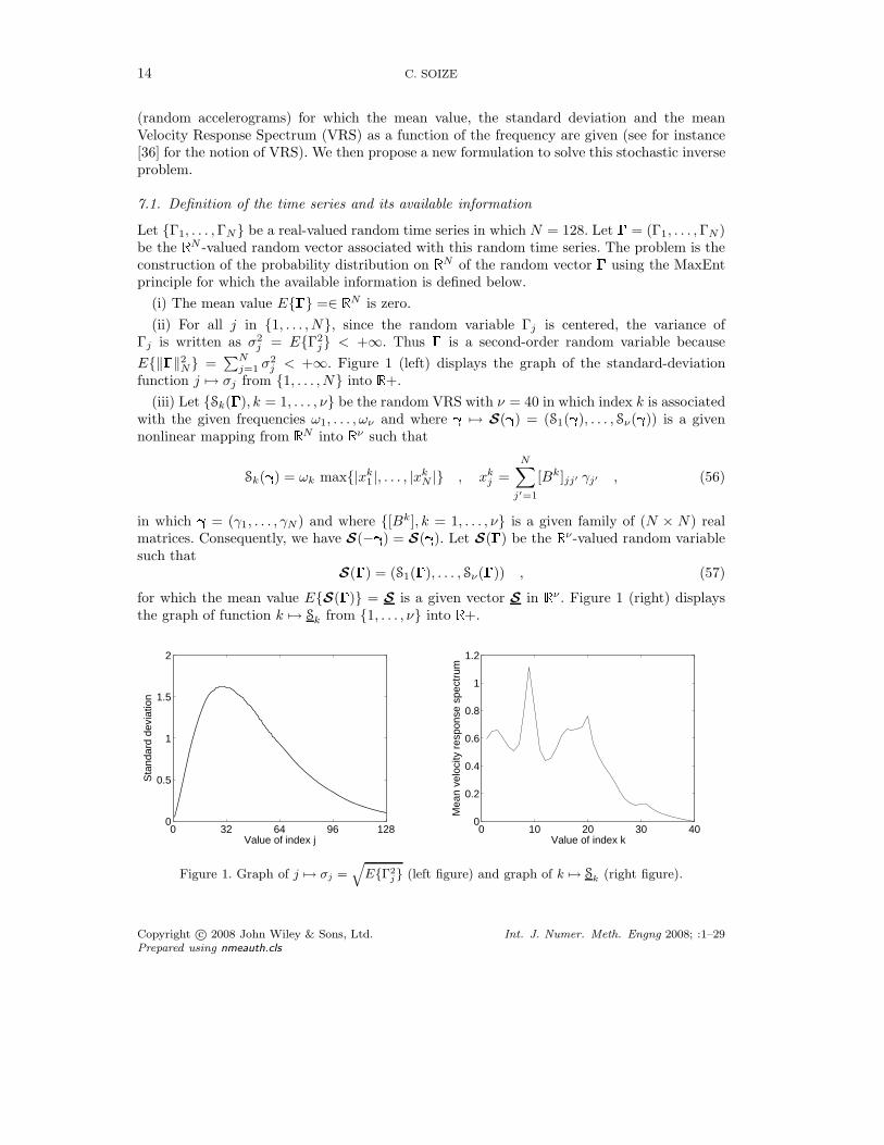
(random accelerograms) for which the mean value, the standard deviation and the meanVelocity Response Spectrum (VRS) as a function of the frequency are given (see for instance[36] for the notion of VRS). We then propose a new formulation to solve this stochastic inverseproblem.

7.1. Definition of the time series and its available information

Let {Γ1, . . . , ΓN} be a real-valued random time series in which N = 128. Let � = (Γ1, . . . , ΓN )be the �N -valued random vector associated with this random time series. The problem is theconstruction of the probability distribution on �

N of the random vector � using the MaxEntprinciple for which the available information is defined below.

(i) The mean value E{�} =∈ �N is zero.

(ii) For all j in {1, . . . , N}, since the random variable Γj is centered, the variance ofΓj is written as σ2

j = E{Γ2j} < +∞. Thus � is a second-order random variable because

E{‖�‖2N} =

∑Nj=1 σ2

j < +∞. Figure 1 (left) displays the graph of the standard-deviationfunction j �→ σj from {1, . . . , N} into �+.

(iii) Let {Sk(�), k = 1, . . . , ν} be the random VRS with ν = 40 in which index k is associatedwith the given frequencies ω1, . . . , ων and where � �→ S(�) = (S1(�), . . . , Sν(�)) is a givennonlinear mapping from �

N into �ν such that

Sk(�) = ωk max{|xk1 |, . . . , |xk

N |} , xkj =

N∑j′=1

[Bk]jj′ γj′ , (56)

in which � = (γ1, . . . , γN ) and where {[Bk], k = 1, . . . , ν} is a given family of (N × N) realmatrices. Consequently, we have S(−�) = S(�). Let S(�) be the �ν-valued random variablesuch that

S(�) = (S1(�), . . . , Sν(�)) , (57)

for which the mean value E{S(�)} = S is a given vector S in �ν . Figure 1 (right) displays

the graph of function k �→ Sk from {1, . . . , ν} into �+.

0 32 64 96 1280

0.5

1

1.5

2

Value of index j

Sta

ndar

d de

viat

ion

0 10 20 30 400

0.2

0.4

0.6

0.8

1

1.2

Value of index k

Mea

n ve

loci

ty r

espo

nse

spec

trum

Figure 1. Graph of j �→ σj =q

E{Γ2j} (left figure) and graph of k �→ Sk (right figure).



7.2. Normalization

In this section we construct the random vector A with values in �N as a normalization of

random vector �. We then construct the probability distribution and the random generatorof A and it will be easy to deduce the probability distribution and the random generator ofrandom vector �. Let A = (A1, . . . , AN ) be the �N -valued random variable defined, for all jin {1, . . . , N}, by Γj =

√N σj Aj . We can then rewrite � as

� =√

N [σ] A , [ σ ]jj′ = σj δjj′ , (58)

in which [ σ ] is a (N×N) real diagonal matrix. The available information introduced in Section7.1 for � allows the corresponding available information for A to be easily deduced.

(i) The mean value E{A} =∈ �N because E{A} = N−1/2 [σ]−1 E{�}. Consequently, A is a

centered random variable,E{A} = . (59)

(ii) For all j in {1, . . . , N}, the second-order moment of random variable Aj is thus equal to1/N and consequently, we have

E{A2j} =

1N

, ∀ j ∈ {1, . . . , N} , (60)

and then E{‖A‖2N} = 1.

(iii) Let s = (s1, . . . , sν) ∈ �ν in which sk = 1 for all k = 1, . . . , ν (all the components of

vector s are equal to 1). Let a �→ s(a) = (s1(a), . . . , sν(a)) be the nonlinear mapping from �N

into �ν such that

sk(a) =Sk(

√N [σ] a)Sk

, ∀ k = 1, . . . , ν . (61)

It can then easily be deduced that

E{s(A)} = s ∈ �ν . (62)

Therefore, the available information which allows the probability distribution of random vectorA to be constructed is maded up of Eqs. (59), (60) and (62).

7.3. Defining the unknown Lagrange multipliers and function Φ

Taking into account the normalization condition for the probability density function pA andthe available information defined by Eqs. (59), (60) and (62), the use of the MaxEnt principleyields

pA(a) = csol0 exp{− < �sol

1 , a >N − < �sol2 , a2 >N − < �sol

3 , s(a) >ν)} , ∀a ∈ �N , (63)

in which a2 denotes the vector (a21, . . . , a

2N) in �

N and where, for the solution, �sol1 ∈ �

N ,�sol

2 ∈ �N and �sol

3 ∈ �ν are the values of the Lagrange multipliers associated with the

constraints defined by Eq. (59), (60) and Eq. (62) respectively. Since S(−�) = S(�) (seeSection 7.1) and from Eqs. (59) and (63), it can be proven that �sol

1 =. Therefore, the Lagrangemultiplier � introduced in Section 2 can be written as � = (�2,�3) ∈ Lμ ⊂ �

μ = �N × �

ν inwhich μ = N + ν and where the admissible set Lμ of � is such that Lμ = (]0 , +∞[)N × �

ν .We then have μ = 168. The mapping a �→ g(a) from �

N into �μ introduced in Section 2 can


16 C. SOIZE

then be written as g(a) = (a2, s(a)) ∈ �N × �

ν = �μ. Let h = (h1, . . . , hN ) be the vector

in �N such that hj = 1/N for all j. Vector f ∈ �

μ introduced in Eq. (2) is then writtenas f = (h, s) ∈ �

N × �ν = �

μ. We use the semi-implicit scheme presented in Section 5.2for the discretization of the Ito stochastic differential equation. Function Φ(u,�) defined byEq. (14) is then written as Φ(u,�) = 1

2 < [K�] u , u>N + ΦNL(u,�) (see Eq. (44)) in whichmatrix [K�] is such that [K�]jj′ = 2{�2}j δjj′ and where ΦNL(u,�) = <�3 , s(u)>ν . For allj fixed in {1, . . . , N}, the generalized partial derivative of function s with respect to uj isrepresented by the function u �→ ∂s(u)/∂uj which is locally bounded on �N . Therefore, for all�2 in (]0 , +∞[)N ⊂ �

N and for all �3 in �ν , Eqs. (23) to (25) are satisfied.

7.4. Computation of the vector-valued Lagrange multipliers using ergodic method

Lagrange multiplier �sol = (�sol2 ,�sol

3 ) ∈ Lμ ⊂ �μ = �

N × �ν are computed in solving Eq. (10)

as explained at the end of Section 2.

(i) The interior-reflective Newton method used to solve Eq. (10) is initialized with �0 =(�0

2,�03) ∈ (]0 , +∞[)N × �

ν = Lμ with �02 = 0.5 η N 1N and �0

3 = 0.5 ν−1(1 − η)N 1ν withη = 0.98 and where 1N and 1ν are the vectors in �

N and �ν for which all the components

are equal to 1. The solution has been calculated in four steps (in order to optimize thecomputer time). For step 1, the parameters are M = 600 and iter = 1, . . . 16 and for step2, are M = 2800 and iter = 17, . . . 30. Figure 2 (right) displays the graph of the functioniter �→ convALG(iter) = ‖E{g(B�(iter))} − f‖2

μ. This calculation is completed by two othersteps, one for which M = 8300 with 7 iterations and the last one for which M = 20000 with7 iterations.

(ii) The mathematical expectation defined by Eq. (11) is estimated by using the ergodicmethod (see Eq. (53)) with M0 = 300 and the semi-implicit scheme presented in Section 5.2is used to construct a realization {Uk(θ), k = 1, . . . , M} of the sequence of the vector-valuedrandom variables {Uk, k = 1, . . . , M} . For each value of vector � = (�2,�3) correspondingto an iteration of the algorithm, the sampling step defined by Eq. (37) has been writtenas Δr = β/m with β = 2π/(

√2λmax

2 ) in which λmax2 = max{(�2)1, . . . , (�2)N} and with

m = 5. Parameter f0 has been fixed to 1. These values of parameters Δr and f0 have beendeduced from a convergence analysis. For instance, Figure 2 (left) displays the graph of thefunction M �→ conv(M) = 1

M

∑Mk=1 ‖Uk(θ)‖2

N for � = �sol and for realization θ. ThereforelimM→+∞ conv(M) = E{‖B�sol‖2

N} = E{‖A‖2N} and we must have limM→+∞ conv(M) = 1

(see Eq. (60)). For M = 20000, we have conv(M) = 0.982 instead of 1 which corresponds toan error of about 1.8%. The convergence is then reasonably reached for M = 20000.

(iii) Figure 3 shows solution �sol and displays the graph of j �→ (�sol2 )j (left figure) and the

graph of k �→ (�sol3 )k (right figure).

7.5. Estimation of the constraints using the Monte Carlo method with the random generator

Solution �sol of Eq. (10) being known, ns independent realizations of random variable A = B�sol

are constructed using the method presented in Section 6.2. The estimation of the mathematicalexpectation E{g(A)} of the constraint is carried out with the Monte Carlo method as explainedin Section 6.3 (see Eq. (55)). Computation is performed with m = 5 (as in Section 7.4),M = 400 and ns = 300. (i) Concerning the value of M , Figure 4 (left) displays the graphof the function M �→ conv�(M) = 1

M

∑Mk=1 ‖Uk(θ�)‖2

N for � = �sol and for a realization θ�



0 10 000 20 0000.7

0.75

0.8

0.85

0.9

0.95

1

1.05

Number M of sampling points

conv

(M)

0 5 10 15 20 25 3010

−4

10−2

100

102

Iteration number

conv

ALG

(iter

) in

log

scal

e

Figure 2. Graph of M �→ conv(M) (left figure) and graph of iter �→ convALG(iter) (right figure).

0 32 64 96 12862

62.5

63

63.5

Index j

Lagr

ange

mul

tiplie

r λ

2sol

0 10 20 30 40−0.2

−0.1

0

0.1

0.2

Index k

Lagr

ange

mul

tiplie

r λ

3sol

Figure 3. Graph of j �→ (�sol2 )j (left figure) and graph of k �→ (�sol

3 )k (right figure).

0 100 200 300 4000

0.2

0.4

0.6

0.8

1


conv

l(M)

0 32 64 96 128−4

−2

0

2

4

Value of index j

Tra

ject

ory

of r

ando

m ti

me

serie

s Γ

Figure 4. Graph of M �→ conv�(M) (left figure) and graph of j �→ Γj(θ�) for a realization θ� (rightfigure).


18 C. SOIZE

0 50 100 150 200 250 3000.7

0.8

0.9

1

1.1

Number ns of realizations

Sec

ond−

orde

r m

omen

t of A

Figure 5. Graph of ns �→ convMC(ns).

0 32 64 96 1280

0.5

1

1.5

2

Value of index j

Sta

ndar

d de

viat

ion

0 10 20 30 400

0.2

0.4

0.6

0.8

1

1.2

Value of index k

Mea

n ve

loci

ty r

espo

nse

spec

trum

Figure 6. Graph of j �→ σj = E{Γ2j}1/2

(left figure) and graph of k �→ Sk (right figure). Reference(dashed lines). Estimation with the random generator (solid lines).

(it should be noted that all the graphs are similar for = 1, . . . , ns). This graph allows thevalue of M to be estimated in order to obtain a realization UM (θ�) of the stationary solutionof the ISDE. Therefore, M must be such that the graph be flat that is reasonably true forM = 400. Therefore Eq. (54) is satisfied in the mean-square sense for M = 400. Figure 4(right) displays the corresponding trajectory of the random time series �, that is to say thegraph of the realization j �→ Γj(θ�) in which �(θ�) =

√N [σ] A(θ�) with A(θ�) UM (θ�).

(ii) Concerning the value of ns, Figure 5 shows the graph of ns �→ convMC(ns) =1

ns

∑ns

�=1 ‖A(θ�)‖2N which is an estimation of the second-order moment E{‖A‖2

N} =E{‖B�sol‖2

N} of the random variable ‖A‖N .

(iii) Figure 6 shows the estimation of the constraints (standard deviation and mean velocityresponse spectrum) constructed with the random generator and compares this estimationwith the references defined in Figure 1. Figure 6 (left) displays the graph of the standard-deviation function j �→ σj from {1, . . . , N} into �+. Figure 6 (right) displays the graph of themean velocity response spectrum k �→ Sk from {1, . . . , ν} into �+. The comparisons are good



and validate the method proposed. The small fluctuations of the estimation of the standard-deviation function computed by the Monte Carlo method using the random generator can bereduced in increasing the value of ns.

8. Construction of a probability model for positive-definite band random matrices

This application is devoted to the construction of a probabilistic model of a band randommatrix with values in the set of all the symmetric positive-definite (n×n) real matrices �+

n (�),for which the available information is made of the mean value, the norm and the norm of itsinverse are given. With such an available information, if the matrix is not a band matrix buta full matrix, an explicit construction can be performed for any value of the matrix dimension(see [8, 9, 10]). If the matrix is a band matrix, such an explicit construction cannot be carriedout and a numerical construction must be done. We then propose hereinafter such a numericalconstruction.

8.1. Definition of the band random matrix and available information

Let [ G ] be the band random matrix with values in �+n (�) with n = 4, for which the band

structure is such that

[ G ] =

⎡⎢⎢⎣

G11 G12 0 0G12 G22 G23 00 G23 G33 G34

0 0 G34 G44

⎤⎥⎥⎦ , (64)

The problem is the construction of the probability distribution on �+n (�) of [ G ] using the

MaxEnt principle for which the available information is defined by

E{[ G ]} = [ In] ,E{‖[ G ] − [ In]‖2

F }‖[ In]‖2

F

= δ2 < +∞ , E{‖[ G ]−1‖2F} = α < +∞ , (65)

in which [ In] is the identity (n × n) matrix, ‖[Mat]‖2F = tr([Mat]T [Mat]) is the square of

the Frobenius norm of the real matrix [Mat], δ = 0.35 which controls the dispersion ofrandom matrix [ G ] and α = 5.6 which must be a positive and finite real number. The firstequation shows that [ G ] is not a centered random variable and its mean value is equal tothe identity matrix. The second equation means that [ G ] is a second-order random variable.By construction, band random matrix [ G ] belongs to �+

n (�) almost surely. Therefore, [ G ]−1

exists almost surely but, in general, is not a second-order random variable that is to say,E{‖[ G ]−1‖2

F } = +∞. This is the reason why the third equation is considered as an availableinformation.

Since [ G ] is positive definite almost surely, random matrix [ G ] can be written (Choleskidecomposition) as

[ G ] = [ L ]T [ L ] , [ L ] =

⎡⎢⎢⎣

A21 A2 0 0

0 A23 A4 0

0 0 A25 A6

0 0 0 A7

⎤⎥⎥⎦ , (66)


20 C. SOIZE

in which A = (A1, . . . , AN ) is a �N -valued random vector with N = 7. Clearly, Eq. (66)

defines a unique nonlinear deterministic mapping a �→ [ G(a) ] from �N into �+

n (�) such that[ G ] = [ G(A) ] and a unique nonlinear deterministic mapping a �→ e(a) from �

N into �N suchthat (G11, G12, G22, G23, G33, G34, G44) = e(A). The problem above is then equivalent to theconstruction of the probability distribution on �

N of the random vector A using the MaxEntprinciple for which the available information is deduced from Eq. (65) and can be rewritten as

E{e(A)} = e ∈ �N , E{‖[ G(A) ]‖2

F} = n(δ2 + 1) , E{‖[ G(A) ]−1‖2F} = α < +∞ , (67)

in which e = (1, 0, 1, 0, 1, 0, 1) ∈ �N .

8.2. Defining the unknown Lagrange multipliers and function Φ

Comparing Eq. (67) with Eq. (2), the nonlinear mapping a �→ g(a) from �N into �μ introduced

in Section 2 can be written as g(a) = (e(a), ‖[ G(a) ]‖2F , ‖[ G(a) ]−1‖2

F ) ∈ �N × � × � = �

μ inwhich μ = N + 2 = 9. Vector f ∈ �

μ introduced in Eq. (2) is written as f = (e, n(δ2 + 1), α).The Lagrange multiplier � introduced in Section 2 can then be written as � = (�1, λ2, λ3) ∈Lμ ⊂ �

μ = �N × �× �. The admissible set Lμ is such that Lμ = �

N×]0 , +∞[×]0 , +∞[. Weuse the explicit Euler scheme presented in Section 5.1 for the discretization of the Ito stochasticdifferential equation. Function Φ(u,�) is then defined by Eq. (14) and for all �1 in �N , for allλ2 and λ3 in ]0 , +∞[, Eqs. (23) to (25) are satisfied.

8.3. Computation of the vector-valued Lagrange multipliers

Lagrange multiplier �sol = (�sol1 , λsol

2 , λsol3 ) ∈ Lμ ⊂ �

μ are computed in solving Eq. (10) asexplained at the end of Section 2. The probability density function defined by Eq. (6) is thenwritten as


1 , e(a) >N −�sol2 ‖[ G(a) ]‖2

F − �sol3 ‖[ G(a) ]−1‖2

F } , ∀a ∈ �N , (68)

(i) The interior-reflective Newton method used to solve Eq. (10) is initialized with �0 =(�0

1, λ02, λ

03) ∈ Lμ ⊂ �

μ with �01 = 1N and λ0

2 = λ03 = 2 where 1N is the vector in �

N forwhich all the components are equal to 1. Figure 7 (right) displays the graph of the functioniter �→ convALG(iter) = ‖E{g(B�(iter))} − f‖2

μ.

(ii) The mathematical expectation defined by Eq. (11) is estimated by using the MonteCarlo method (see Eq. (55)), the random generator (see Eq. (54)) with the Explicit Eulerscheme presented in Section 5.1. For any value of vector � corresponding to an iterationof the algorithm, parameter f0 is fixed to 1 and the sampling step defined by Eq. (37)is deduced from a convergence analysis and is written as Δr = β/m with β = 1 andm = 5. Concerning the value of M , Figure 7 (left) displays the graph of the functionM �→ conv�(M) = 1

M

∑Mk=1 ‖Uk(θ�)‖2

N for � = �sol and for a realization θ� (it should benoted that all the graphs are similar for = 1, . . . , ns and for any admissible value of vector�). This graph allows the value of M to be estimated in order to obtain a realization UM (θ�)of the stationary solution of the ISDE. Therefore, M must be such that the graph be flat thatis reasonably true for M = 5000. Therefore Eq. (54) is satisfied in the mean-square sense forM = 5000.



(iii) The value of ns has also been deduced from a convergence analysis. For instance,at solution � = �sol, Figures 8 (left and right) show the graphs of ns �→ δ(ns) such that1

ns

∑ns

�=1 ‖[ G(A(θ�)) ]‖2F = n(δ(ns)2 + 1) and ns �→ α(ns) = 1

ns

∑ns

�=1 ‖[ G(A(θ�)) ]−1‖2F =

n(δ(ns)2 + 1) An excellent convergence is obtained for ns = 600 which is the value used in thecomputation.

(iv) Concerning solution �sol, we get �sol1 = (0.7381, 4.1697, 1.2465,−0.9248, 0.8998, 4.2584,

0.8714), λsol2 = 2.2293 and λsol

3 = 1.7749.

0 1000 2000 3000 4000 50003

3.5

4

4.5

5


Con

v l(M)

1 2 3 4 5 6 710

−4

10−2

100

Iteration number iterC

onvA

LG(it

er)

in lo

g sc

ale

Figure 7. Graph of M �→ conv�(M) (left figure) and graph of iter �→ convALG(iter) (right figure).

0 100 200 300 400 500 6000

0.1

0.2

0.3

0.4

0.5


δ (n

s)

0 100 200 300 400 500 6005.2

5.4

5.6

5.8

6

6.2


α (n

s)

Figure 8. Graph of ns �→ δ(ns) (left figure) and graph of ns �→ α(ns) (right figure).

8.4. Estimation of the constraints with the random generator

Solution �sol of Eq. (10) being known, ns independent realizations of random variable A = B�sol

are constructed using the random generator presented in Section 6.2 (exactly, as we haveperformed to calculate �sol in Section 8.3). The estimations of the mathematical expectationsE{g(A)} of the constraints are calculated by the Monte Carlo method as explained in Section


22 C. SOIZE

6.3 (see Eq. (55)) and as performed above in Section 8.3. Computation is then performed withf0 = 1, m = 5, M = 5000 and ns = 600.

(i) Concerning the estimation of the constraints, we obtain

E{[ G ]}

⎡⎢⎢⎣1.0001 0.0051 0 00.0051 0.9910 0.0057 0

0 0.0057 1.0222 0.00770 0 0.0077 1.0056

⎤⎥⎥⎦ , (69)

which has to be compared to the identity matrix, δ 0.3529 which has to be compared to0.3500 and finally, α 5.6053 which has to be compared to 5.6000. We then have a goodcomparison.

9. Extension of the theory to the case of a probability density function with any support andapplication to the Karhunen-Loeve expansion of a Non-Gaussian positive-valued random

field

In a first subsection, we show how the previous developments can be used for a probabilitydensity function for which its support is not �N but is any part A of �N . The second subsectionwill deal with an application devoted to the construction of the Karhunen-Loeve expansion ofa subclass of Non-Gaussian positive-valued random fields for which the general class has beenintroduced and analyzed in [37].

9.1. Extension of the theory to a probability density function with any support

Let A be any part of �N , x = (x1, . . . , xN ) be any vector in �N and let dx = dx1 . . . dxN be

the Lebesgue measure on �N . Let X = (X1, . . . , XN ) be a �

N -valued second-order randomvariable for which the probability distribution PX(dx) = pX(x) dx on �

N is unknown and isrepresented by a probability density function x �→ pX(x) from �

N into �+ whose support is

A ⊂ �N (consequently, pX(x) = 0 for all x /∈ A). We then have

Supp pX = A ,

∫�N

pX(x) dx =∫

A

pX(x) dx = 1 . (70)

The problem to be solved is the construction of pX using the MaxEnt principle for which theconstraints associated with the available information (see Eq. (2)) is

E{g(X)} = f , (71)

in which f = (f1, . . . , fμ) is a given vector in �μ and where x �→ g(x) = (g1(x), . . . , gμ(x)) is a

given measurable mapping from �N into �μ. We then obtain (see Section 2 and Eq. (6)),

pX(x) = �A(x) csolX exp(− < �sol, g(x) >μ) , ∀x ∈ �

N , (72)

in which �A(x) = 1 if x ∈ A and �A(x) = 0 if x /∈ A and where csolX = exp(−λsol

0 ) is theconstant of normalization calculated with Eq. (70). It should be noted that we cannot directlyused the previous theory in introducing the function Φ(u,�) = − ln(�A(u))+ < �, g(u) >μ

(see Eq. (14)) because the function u �→ ‖∇uΦ(u,�)‖N is not a locally bounded function on�

N (it is a distribution or a generalized function). We must then proceed differently.



Note that (1) the calculation of the cumulative distribution function (probabilitydistribution) or the calculation of the moments for the random responses of the computationalmodel or (2) the calculation of the left-hand side of Eq. (71) lead us to calculate quantitiesof the type E{h(X)} in which x �→ h(x) is a given vector-valued function defined on �

N . LetpA be the probability density function of the �N -valued random variable A = (A1, . . . , AN )defined in Section 2 and constructed using the method presented in Sections 3 to 6. We thenhave

E{h(X)} =∫�N

h(x)�A(x) csolX exp(− < �sol, g(x) >μ) dx , (73)

which can be rewritten as

E{h(X)} =csolX

csol0

∫�N

h(a)�A(a) pA(a) da , (74)

in which pA is defined by Eq. (6). Taking h(a) = 1, it can be deduced that csolX /csol

0 =1/E{�A(A)}. Finally, E{h(X)} can be calculated by

E{h(X)} =E{h(A)�A(A)}

E{�A(A)} , (75)

where the mathematical expectations in the right-hand side of Eq. (75) are calculated by thetheory developed in Sections 2 to 6.

Remark. It should be noted that the proposed method consists in solving the problem on anunconstrained support and then in restricting the solution on the desired support A, rescalingthe probability density function. This implies that the solution on the unrestricted supportexists, that is to say that the function x �→ g(x) = (g1(x), . . . , gμ(x)) from �

N into �μ be suchthat the conditions defined by Eqs. (23) to (25) hold. This is the case for the fundamentalapplication presented below for which the proposed method is very efficient. Nevertheless,such a solution may not exist. In order to explain the difficulties and to give a few ideas toconstruct the solution in such a case, we then propose to analyze below the ”extreme” casefor which the probability density function is uniform on a compact support A. In this caseg is zero and Eq. (72) yields pX(x) = �A(x) csol

X for all x in �N . Clearly, the solution pA on

the unrestricted support �N does not exist. To analyze such a case, a regularization gε of thefunction g depending on a parameter ε > 0 can be introduced such that, for all ε > 0, (1)the function x �→ gε(x) is differentiable on �

N , (2) for all x in A, we have gε(x) = 0, (3) theconditions defined by Eqs. (23) to (25) hold for gε and (4) the support of gε(x), which is �N

tends to the compact support A when ε goes to zero. Such a regularization is not always easyto construct, but if it is possible, then this method is very efficient. In order to illustrate sucha method, let us consider the simple case for which N = 1 and A = [−1 , +1]. We can thechoose the following regularization: gε(x) = 0.5 ε−2(x − 1)2 if x > 1, gε(x) = 0 if x ∈ A andgε(x) = 0.5 ε−2(x + 1)2 if x < −1. In this case, x �→ dgε(x)/dx is a continuous function on �

such that dgε(x)/dx = ε−2(x−1) if x > 1, dgε(x)/dx = 0 if x ∈ A and dgε(x)/dx = ε−2(x+1)if x < −1. Then for ε sufficiently small (but not to small), the method would be very efficient.

9.2. Application to the Karhunen-Loeve expansion of a Non-Gaussian positive-valued randomfield

We consider the following computational model resulting from the finite element discretizationof an elliptic boundary value problem (for instance, a linear elastostatic problem on a bounded


24 C. SOIZE

3D domain) and written as

[K] Y = r , [K] =n∑

j=1

Zj [kj ] , (76)

in which Z = (Z1, . . . , Zn) is the spatial sampling of a positive-valued random field (forinstance, the Young modulus in linear isotropic elasticity for a heterogeneous material), where[k1], . . . , [kn] are n given symmetric real matrices, where r is a given vector and where Y isthe unknown random vector. The random matrix [K] is assumed to be positive-definite almostsurely (a.s) and consequently, Y = [K]−1 r almost surely. The mean value z = (z1, . . . , zn) of Zis z = E{Z}. Since Z corresponds to the sampling of a positive-valued random field, then forall j ∈ {1, . . . , n}, it is assumed that zj > 0 and Zj > 0 almost surely. We then introduce thenormalized random vector G = (G1, . . . , Gn) with values in �

n such that Zj = zj Gj for allj ∈ {1, . . . , n}. Therefore, we have Gj > 0 almost surely for all j ∈ {1, . . . , n}. The probabilitydistribution of random vector G must be such that Y is a second-order random variable, i.eE{‖Y‖2} = cY < +∞. Using similar developments to those given in Ref. [37] and taking intoaccount that for all g1 > 0, . . . , gn > 0, we have

(max{ 1g1

, . . . ,1gn

})2 ≤ 1g21

+ . . . +1g2

n

, (77)

it can be proven that E{‖Y‖2} = cY < +∞ if the following inequality holds,

E{ 1G2

1

+ . . . +1

G2n

} = cG < +∞ . (78)

The Karhunen-Loeve expansion GN at order N of the random field G yields the followingapproximation for the �n-valued random vector G,

GN = G +N∑

α=1

√vα Xα �

α , (79)

in which G = (G1, . . . , Gn) with Gj = 1 for all j. In Eq. (79), �1, . . . ,�N are the orthonormaleigenvectors (<�α ,�β >= δαβ) associated with the N largest eigenvalues v1 > v2 > . . . > vN

of the covariance matrix [CG] = E{(G − G) (G − G)T } of G which is assumed to be given.For the construction by the MaxEnt principle of the probability distribution on �

N of thesecond-order �N -valued random variable X = (X1, . . . , XN ), the available information is thefollowing,

Supp pX = A ⊂ �N , (80)

E{X} = 0 , (81)

E{X XT } = [IN ] , (82)

E{s(X)} = κ < +∞ , (83)

in which for all x = (x1, . . . , xN ) ∈ A, we have

s(x) =n∑

j=1

(Gj +N∑

α=1

√vα xα ϕα

j )−2 . (84)



The support A of pX is defined by

A = {x ∈ �N such that ∀j ∈ {1, . . . , n} , Gj +

N∑α=1

√vα xα ϕα

j > 0} . (85)

The nonlinear mapping x �→ g(x) from �N into �μ introduced in Section 2 can be written as

g(x) = (x , e(x) ,1κ

s(x)) , (86)

in which μ = N + N(N + 1)/2 + 1 and where e(x) is a vector in �N(N+1)/2 constituted of

the elements (stored column rise) of the upper triangular part (including the diagonal) of thematrix x xT . The vector f in �

μ introduced in Eq. (71) is then written as

f = (0N , e , 1) , (87)

in which 0N = (0, . . . , 0) ∈ �N and where e = E{e(X)} is the vector in �

N(N+1)/2 constitutedof the elements (stored column rise) of the upper triangular part (including the diagonal) ofthe matrix [IN ] (and consequently, constituted of 0 and 1).

The Lagrange multiplier � introduced in Section 2 can then be written as � = (�1,�2, λ3) ∈Lμ ⊂ �

μ = �N × �

N(N+1)/2 × �. The semi-implicit scheme defined is Subsection 5.2 is usedto discretize the Ito stochastic differential equation. Function Φ(u,�) is defined by Eq. (44) inwhich matrix [K�] is such that, for all u in �

N ,

< �2 , e(u) >N(N+1)/2=

12

< [K�] u , u >N , (88)

and vector LNL(u) is given by

LNL(u) = −�1 − λ3

κ∇us(u) . (89)

The gradient ∇us(u) = (∂s(u)∂u1

, . . . , ∂s(u)∂uN

) at point u = (u1, . . . , uN) is such that, for allα ∈ {1, . . . , N},

∂s(u)∂uα

= −2n∑

j=1

√vαϕα

j

(Gj +∑N

β=1

√vβ uβ ϕβ

j )3. (90)

It should be noted that the subset of the admissible values of �2 is such that [K�] is a positive-definite matrix and the subset of the admissible values of λ3 is ]0 , +∞[. Since the value of κis arbitrary, λ3 can be fixed to a given value denoted by λsol

3 . The Lagrange multipliers �sol1

and �sol2 are computed in solving Eq. (71) by using Eq. (75). The probability density function

defined by Eq. (6) is written as


1 , a) >N − < �sol2 , e(a) >

N(N+1)/2 −λsol3 s(a)} , ∀a ∈ �

N , (91)

For the numerical application, n = 100 and the values of√

v1, . . . ,√

v20 are respectively,2.78, 1.18, 0.82, 0.48, 0.38, 0.28, 0.23, 0.21, 0.18, 0.17, 0.15, 0.14, 0.13, 0.11, 0.106, 0.102,0.09, 0.088, 0.081, 0.080. Figure 9 displays the graph of the function N �→ error(N) =E{‖G − GN‖2/E{‖G‖2} = (tr{[CG]} − ∑N

α=1 vα)/tr{[CG]} which allows the error to bemeasured when G is replaced by the K-L expansion GN . It can be seen that N = 10 implies


26 C. SOIZE

0 5 10 15 2010

−3

10−2

10−1

100

Dimension of the KL expansion N

Err

or(N

) in

log

scal

e

Figure 9. Graph of N �→ error(N) showing the convergence of Karhunen-Loeve expansion.

0 2 4 6

x 105

0

5

10

15


Con

v(M

)

0 1 2 3 4 5 6 7 8 9 10−25

−20

−15

−10

−5

0

5

Iteration number iter

Con

vALG

(iter

) in

log

scal

e

Figure 10. Graph of M �→ conv(M) (left figure) and graph of iter �→ convALG(iter) (right figure).

a reasonable relative error. The mathematical expectations in Eq. (75) are estimated byusing the ergodic theory (see Eq. (53)) and the semi-implicit scheme is used to construct arealization {Uk(θ), k = 1, . . . , M} of the random variables {Uk, k = 1, . . . , M}. The samplingstep defined by Eq. (37) is taken as Δr = 0.01. Parameter f0 is equal to 0.5, M0 = 200, 000and M = 600, 000. These values of parameters Δr, f0, M0 and M have been derived from aconvergence analysis. The value of λ3 is fixed to the value λsol

3 = 0.01 and Eq. (71) is solvedwith respect to (�1,�2) by using the trust-region dogleg algorithm which is a variant of thePowell dogleg method. The initial values used are �0

1 = 0.8 �N and �02 = 0.2 e. Figure 10 (left)

displays the graph of the function M �→ conv(M) showing the convergence of the estimationof E{‖B

e�sol‖2N} by using the ergodic method with � = (�1,�2). Figure 10 (right) displays the

graph of the function iter �→ convALG(iter) = ‖E{g(Be�(iter))}− f‖2

μ−1 showing the convergenceof trust-region dogleg algorithm in function of the iteration number. Figure 11 (left) comparesthe graph α �→ (�sol

1 )α of the solution for �1 with the graph α �→ (�01)k of the initial value

�01 = 0.8 �N . Figure 11 (right) compares the graph k �→ (�sol

2 )k of the solution for �2 with the



1 2 3 4 5 6 7 8 9 10−0.5

0

0.5

1

1.5

Index α

λ 1sol (α

)

1 6 11 16 21 26 31 36 41 46 51 55−0.1

0

0.1

0.2

0.3

0.4

0.5

Index k

λ 2sol (k

)

Figure 11. Left figure: Graph of α �→ (�sol1 )α (circle marker) and graph of α �→ (�0

1)α (dot marker).

Right figure: Graph of k �→ (�sol2 )k (circle marker) and graph of k �→ (�0

2)k (dot marker).

graph k �→ (�02)k of the initial value �0

2 = 0.2 e. For the solution obtained �sol = (�sol1 ,�sol

2 , λsol3 )

with λsol3 = 0.01, Eq. (81) and Eq. (82) are satisfied at 10−11 for each components and Eq. (83)

yields κ = 140.027. The results obtained are thus very good.

10. Conclusions

We have proposed a method to effectively construct the probability density function of arandom variable in high dimension and for any support of its probability distribution by usingthe MaxEnt principle. To calculate the integrals of the problem in high dimension and toconstruct a generator of independent realizations, an alternative algorithm to the Metropolis-Hastings or Gibbs algorithms is proposed. This algorithm is derived from the discretizationof an Ito stochastic differential equation for which the stability, the speed of convergenceand the transient part can be controlled. The method proposed is validated through threefundamental applications. The first one is a new formulation of the stochastic inverse problemconsisting in constructing the probability distribution in high dimension and of its generatorfor a vector-valued random variable corresponding to an unknown non-stationary random timeseries (random accelerograms) for which the Velocity Response Spectrum is given. The secondone is also a new formulation related to the construction of the probability distribution inhigh dimension and of its generator for positive-definite band random matrices. Clearly, themethod proposed can be used for any sparse random matrix. Finally, we present an extensionof the theory when the support of the probability distribution in high dimension of the randomvariable is not all the space but is any part of the space. The third application is then a newformulation related to the construction of the probability distribution in high dimension forthe Karhunen-Loeve expansion of Non-Gaussian positive-valued random fields.

REFERENCES


28 C. SOIZE

1. Schueller GI (editor). A state-of-the-art report on computational stochastic mechanics. ProbabilisticEngineering Mechanics 1997; 12(4):197-321.

2. Schueller GI. Computational stochastic mechanics - recent advances. Computers & Structures 2001; 79(22-25):2225-2234.

3. Wiener N. The Homogeneous Chaos. American Journal of Mathematics 1938; 60: 897-936.4. Spanos PD, Ghanem R. Stochastic finite element expansion for random media. Journal of Engineering

Mechanics, ASCE 1989; 115(5):1035-1053.5. Ghanem R, Spanos PD. Stochastic Finite Elements: A spectral Approach. Springer-Verlag: New York, 1991.6. Ghanem R. Ingredients for a general purpose stochastic finite elements formulation. Computer Methods in

Applied Mechanics and Engineering 1999; 168:19-34.7. Soize C, Ghanem R. Physical systems with random uncertainties : Chaos representation with arbitrary

probability measure. SIAM Journal On Scientific Computing 2004; 26(2):395-410.8. Soize C. A nonparametric model of random uncertainties for reduced matrix models in structural dynamics.

Probabilistic Engineering Mechanics 2000; 15(3):277-294.9. Soize C. Maximum entropy approach for modeling random uncertainties in transient elastodynamics.

Journal of the Acoustical Society of America 2001; 109(5):1979-1996.10. Soize C. Random matrix theory for modeling uncertainties in computational mechanics. Computer Methods

in Applied Mechanics and Engineering 2005; 194(12-16):1333-1366.11. Shannon CE. A mathematical theory of communication. Bell System Technology Journal 1948; 27:379-423

& 623-659.12. Jaynes ET. Information theory and statistical mechanics. Physical Review 1957; 106(4):620-630 &

108(2):171-190.13. Serfling RJ. Approximation Theorems of Mathematical Statistics. John Wiley & Sons: New York, 1980.14. Kapur JN, Kesavan HK. Entropy Optimization Principles with Applications. Academic Press: San Diego,

1992.15. Jumarie G. Maximum Entropy, Information Without Probability and Complex Fractal. Kluwer Academic

Publishers: Dordrecht, 2000.16. Sobczyk K, Trebicki J. Maximum entropy principle in stochastic dynamics. Probabilistic Engineering

Mechanics 1990; 5(3):102-110.17. Mead LR., Papanicolaou N. Maximum entropy in the problem of moments. J. Math. Phys. 1984;

25(8):2404-2417.18. Ciulli S, Mounsif M. On the application of maximum entropy to the moments problem. J. Math. Phys.

1991; 32(7):1717-1719.19. Tagliani A. Maximum entropy in the Hamburger moments problem. J. Math. Phys. 1994; 35(9):5087-5096.20. Volpe EV, Baganoff D. Maximum entropy pdfs and the moment problem undear near-Gaussian conditions.

Probabilistic Engineering Mechanics 2003; 18(3):17-29.21. Coleman TF, Li Y. On the convergence of reflective newton methods for large-scale nonlinear minimization

subject to sounds. Mathematical Programming 1994; 67(2):189-224.22. Coleman TF, Li Y. An interior, trust region approach for nonlinear minimization subject to bounds. SIAM

Journal on Optimization 1996; 6:418-445.23. Ergorov AD, Sobolevsky PI, Yanovich LA. Functional Integrals: Approximate Evaluation and Applications.

Kluwer Academic Publisher: Dordrecht, 1993.24. MacKeown PK. Stochastic Simulation in Physics. Springer-Verlag: Singapore, 1997.25. Hastings WK. Monte Carlo sampling methods using Markov chains and their applications. Biometrika

1970; 109:57-97.26. Kaipio J, Somersalo E. Statistical ans Computational Inverse Problems. Springer-Verlag, New York, 2005.27. Spall JC. Introduction to Stochastic Search and Optimization. John Wiley and Sons: Hoboken, New Jersey,

2003.28. Geman S, Geman D. Stochastic relaxation, Gibbs distribution and the Bayesian distribution of images.

IEEE Transactions on Pattern Analysis and Machine Intelligence 1984; Vol PAM I-6:721-741.29. Mehta ML. Random Matrices, Revised and Enlarged Second Edition. Academic Press: New York, 1991.30. Soize C. The Fokker-Planck Equation for Stochastic Dynamical Systems and its Explicit Steady State

Solutions. World Scientific: Singapore, 1994.31. Caughey TK. Derivation and application of the Fokker-Planck equation to discrete nonlinear dynamic

systems subjevted to white random excitation. The Journal of The Acoustical Society of America 1963;35(11):1683-1692.

32. Yosida K. Functional Analysis. Springer-Verlag: Berlin, 1995.33. Talay D, Tubaro L. Expansion of the global error for numerical schemes solving stochastic differential

equation. Stoch. Anal. Appl. 1990; 8(4):94-120.34. Kloeden PE, Platen E. Numerical Solution of Stochastic Differential Equations. Springer-Verlag: Berlin,

1992.



35. Talay D. Stochastic Hamiltonian system: exponential convergence to the invariant measure anddiscretization by the implicit Euler scheme. Markov Processes and Related Fields 2002; 8:163-198.

36. Clough RW., Penzien J. Dynamics of Structures. McGraw-Hill: New York, 1975.37. Soize C. Non Gaussian positive-definite matrix-valued random fields for elliptic stochastic partial differential

operators. Computer Methods in Applied Mechanics and Engineering 2006; 195:26-64.


construction of probability distributions in high

Documents