constructioncontingency200409

8/22/2019 ConstructionContingency200409

http://slidepdf.com/reader/full/constructioncontingency200409 1/16

COBRA 2004The international construction research conference of theRoyal Institution of Chartered Surveyors

7-8 September 2004

Leeds Met

ropolita

n Un

iversit

y



COBRA 2004 was held on 7-8 September 2004 atHeadingley Cricket Club, Leeds.

It was organised by the School of the Built Environment, Leeds MetropolitanUniversity and the Yorkshire and Humberside Region of The Royal Institutionof Chartered Surveyors.

The proceedings were edited by Robert Ellis and Malcolm Bell of LeedsMetropolitan University.

COBRA 2004 sponsors were:

• White Young Green

• Faithful and Gould Worldwide• Hays Montrose

ISBN 1-842-19193-3



ACCURACY IN ESTIMATING PROJECT COST

CONSTRUCTION CONTINGENCY – A STATISTICALANALYSIS

David Baccarini

Department of Construction Management, Curtin University of Technology,

PO Box U1987, Perth 6845, Western Australia, Australia

ABSTRACT

The cost performance of building construction projects is a key success criterion for project sponsors. Project cost performance is typically measured by comparing finalcost against budget. A key component of the project budget for the constructioncontract is construction contingency, which caters for contract variations that ariseduring the implementation phase of projects. It is important for project sponsors to

know the level of accuracy being achieved in estimating construction contingency.Statistical analysis of past projects provides a means for measuring the accuracy of construction contingency. The cost data for 48 road construction projects completed

by an Australian government organisation were statistically analysed to investigate theaccuracy of contingency. It was found that the average construction contingency was5.24% of the Award Contract Value but the average value of contract variations was9.92%. The organisation used a traditional percentage approach for estimatingconstruction contingency. This suggests that the organisation has room to improve theaccuracy of its construction contingency estimates by seeking alternative estimatingmethods. An investigation of an alternate estimating approach derived from theanalysis of the data found that there were no significant correlations between projectvariables and construction contingency that might be used to create a prediction modelfor construction contingency.

Keywords: cost contingency, project cost performance, risk management.

INTRODUCTION

The cost performance of construction projects is a key success criterion for projectsponsors Construction projects are notorious for running over budget (Hester et al



"An amount of money or time (or other resources) added to the base estimatedamount to (1) achieve a specific confidence level, or (2) allow for changes that

experience shows will likely be required" (AACE 2000: 28)

“The amount of money or time needed above the estimate to reduce the risk of overruns of project objectives to a level acceptable to the organization” (PMI2000: 199)

The key attributes of the concept of project cost contingency are:

• Reserve - Cost contingency is a reserve of money (AACE 2000).

• Risk – The need and amount for contingency reflects the existence of risk in projects (Thompson & Perry, 1992). Contingency covers for two categories of risks – known unknowns and unknown unknowns (PMI 2000, Hillson 1999).Contingency caters for events within the defined project scope that are unforeseen(Moselhi 1997, Yeo 1990), unexpected (Mak et al 1998), unidentified (Levine1995), or undefined (Clark and Lorenzoni 1985, Thompson and Perry 1992).

• Risk Management – There is a range of risk management strategies for risk in

projects such as risk transfer, risk reduction, and financial treatments for retainedrisks e.g. contingency (Standards Australia 1999). So contingency is used inconjunction with other risk treatment strategies.

• Total Commitment - Cost estimates are prepared and contingencies added in order to indicate the likely total cost of the project. The inclusion of contingencies withina budget estimate means that the estimate represents the total financial commitmentfor a project.

• Project Outcomes - Contingency can have a major impact on project outcomes for a project sponsor. If contingency is too high it might encourage sloppy costmanagement, cause the project to be uneconomic and aborted, and lock up fundsnot available for other organisational activities; if too low it may be too rigid andset an unrealistic financial environment, and result in unsatisfactory performanceoutcomes (Wideman 1995, Dey et al 1994).

Two major categories of contingency can be identified for construction projects (HM

Treasury, 1993):• Design Contingency – this is for changes during the design process for such

factors as incomplete scope definition and inaccuracy of estimating methods anddata (Clark & Lorenzoni, 1985).

• Construction Contingency - this is for changes during the construction process.Under a traditional procurement arrangement the project sponsor procures



RESEARCH DESIGN

Construction contingency is the focus of the research reported within this paper.Figure 1 set outs a model for estimating construction contingency by the projectsponsor prior to the commencement of construction phase of projects. The sponsor needs an estimate of the final cost of the project for budgeting purposes. This budgetis a combination of the awarded contract value plus construction contingency.Key elements of this model are:1. Contingency estimating methods - There are numerous estimating methods

available for project cost contingency. Traditionally cost estimates have beentreated as being deterministic [i.e. point estimates for each cost element] based ontheir most likely value (Mak et al 1998). Contingencies are often calculated as anacross-the-board percentage addition on the base estimate, typically derived fromintuition, past experience and historical data. This approach is consideredarbitrary, as Thompson and Perry (1992:1) observe, “all too often risk is either ignored or dealt with in an arbitrary way: simply adding a 10% 'contingency' ontothe estimated cost of a project is typical". And it is difficult for the estimator to

justify or defend (Newton 1992, Yeo 1990). It is an unscientific approach and a reason why so many projects are over budget (Hartman 2000). Nowadays moresophisticated estimating methods are available, such as Monte Carlo simulationand artificial neural networks.

2. Influential variables - There are several variables that may influence theestimating process and the amount of estimated contingency (e.g. organisational,

project, cognitive).3. Contingency Accuracy - Construction contingency is added to the award contract

value to represent the sponsor’s predicted final cost of the project. The actual finalcost is the award contract value plus/minus contractual variations. The accuracy of the contingency can be measured by comparing the predicted final cost against theactual final cost.

Using the model in Figure 1, the following two research questions for estimatingaccurate project cost contingency can be identified:

1. How accurate are construction contingencies?2. What project variables are correlated with construction contingency so that a

predictive model for estimating construction contingency can be derived?

So, the objectives of the research are to quantitatively analyse cost data of completedconstruction projects to attempt to answer these research questions.



cost contingency as ‘provisional sum,’ which is defined as an amount of money setaside to cater for the uncertainty associated with the delivery of the project. The

organisation uses a traditional percentage approach to calculate contingency.

Sample

The research population consisted of road construction project sponsored by the casestudy organisation. The selection of a research sample of 48 projects was derived

based on the following criteria:1. The time span for the sample was from 1997 to 2002, because cost data was

readily accessible between these years. Ten projects were randomly identifiedfrom each year to provide a sample of 50. A review of the sample identifiedtwo projects as outliners that would distort the analysis. Therefore 48 projectswere analysed.

2. All sample projects had reached practical completion.3. All sample projects used traditional procurement with open competitive

tendering using the Australian Standard AS 2124 – 1992, General Conditions

of Contract.4. Sample projects included areas in all regions of the state.5. The range of dollar value was from A$0.05m to over A$35m

The following information was obtained for each project in the sample:

• Date of bid

• Location

• Project Duration

• Number of Bidders

• Mean Value of Bids

• Award Contract Value

• Final Contract Value

• Variations Value

• Contingency

The data obtained was statistically analysed using SPSS (Statistical Package for theSocial Sciences) software. Two forms of statistical analysis were undertaken:o Descriptive statistics - This provided general statistical information such as the

mean, standard deviation and co-efficient of variation of variables.o Correlation - Correlation to examine the relationship between two variables (bi-

variate)



ACCURACY OF CONSTRUCTION CONTINGENCY

Construction contingency caters for variations allowable under the contract betweenthe sponsor and contractor (Mak & Picken, 2000). A comparison of predicted finalcost against actual final cost indicates the accuracy of contingency. Broadly, thesmaller the difference between these two costs the more ‘accurate’ the contingencyvalue. This would indicate whether there is a problem is accurately estimating projectcost contingency.

Measurement of Contingency Accuracy

Contingency Accuracy (CA) is measured by comparing construction contingency andapproved contract variations, expressed as a percentage of Award Contract Value:

CA = ΣV% - ΣC%

Where:

ACV = Award Contract Value (successful construction tender, expressed in A$)C% = Construction Contingency, expressed as % of ACVV% = Variations, expressed as % of ACV

In order to measure Contingency Accuracy, variables C% and V% need to becalculated.

Contingency (C%)

Contingency (C%) is the ratio of the construction contingency to the ACV, expressedas a percentage:

C% = ΣC x 100ΣACV

Where:

C = Construction contingency, expressed in A$

Table 1 displays the range of contingency (C%) in the sample projects. It shows thatconstruction contingency averaged 5.24% of ACV. The variability is relativelylimited, suggesting that the traditional percentage approach to estimating results inconservative estimates, anchored around 5-10%.



Variation (V%)

Variation (V%) is the ratio of the value of contract variations to the Award ContractValue (ACV), expressed as a percentage:

V (%) = Σ V x 100Σ ACV

Where:V = approved contract variations, expressed in $A

Table 2 displays the results for variation (V%). Of the 48 projects, variationsdecreased the ACV in 7 projects and increased the ACV in 41 of projects. The averagevariation (V%) for all projects was 9.92% of ACV. The variability for variations(V%), as measured in terms of standard deviation and co-efficient of variation, ismuch greater than the variability for construction contingency (C%). This indicatesthat the estimation of contingency is not fully reflecting the variability of contractvariations.

Variation(%)

Nr of Projects(n=48)

>-20% 1

-15.01_-20% 1

-10.01_-15% 0

-5.01_-10% 3

0.00_-5% 2

0.00_5 % 14

5.01_10% 1410.01_15% 4

15.01_20% 4

>20% 5

9.92% Mean

21% Std Devn.

208% Coef. of Var.

Table 2: Variation (V%)

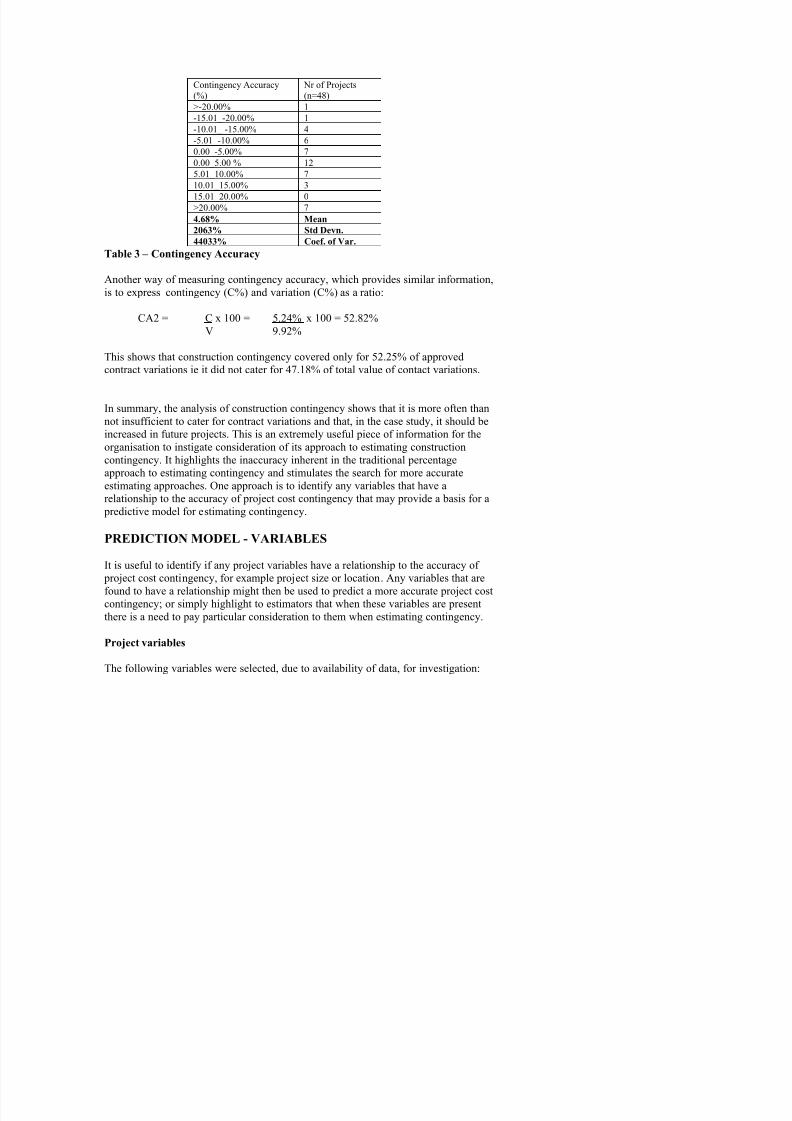
Contingency Accuracy (CA)

As stated previously, Contingency Accuracy can be expressed as the difference between Contingency and Variation, thus:



Contingency Accuracy

(%)

Nr of Projects

(n=48)>-20.00% 1

-15.01_-20.00% 1

-10.01_ -15.00% 4

-5.01_-10.00% 6

0.00_-5.00% 7

0.00_5.00 % 12

5.01_10.00% 7

10.01_15.00% 3

15.01_20.00% 0>20.00% 7

4.68% Mean

2063% Std Devn.

44033% Coef. of Var.

Table 3 – Contingency Accuracy

Another way of measuring contingency accuracy, which provides similar information,

is to express contingency (C%) and variation (C%) as a ratio:

CA2 = C x 100 = 5.24% x 100 = 52.82%V 9.92%

This shows that construction contingency covered only for 52.25% of approvedcontract variations ie it did not cater for 47.18% of total value of contact variations.

In summary, the analysis of construction contingency shows that it is more often thannot insufficient to cater for contract variations and that, in the case study, it should beincreased in future projects. This is an extremely useful piece of information for theorganisation to instigate consideration of its approach to estimating constructioncontingency. It highlights the inaccuracy inherent in the traditional percentageapproach to estimating contingency and stimulates the search for more accurate

estimating approaches. One approach is to identify any variables that have arelationship to the accuracy of project cost contingency that may provide a basis for a predictive model for estimating contingency.

PREDICTION MODEL - VARIABLES



Project Size

Project size can be measured in terms of financial value. Table 4 categorises projects by ACV, which is the value of the successful tender. The ACV ranged from $57,000to $ 34,000,000. The mean ACV was $5,462,742.10 and the majority of projects(58%) below $4,000,000.

Award Contract Value(A$)

Nr of Projects(n = 48)

<$2.00m 21

$2.01_4.00m 7$4.01_6.00m 4

$6.01_8.00m 5

8.01_10.00m 4

>$10.00m 7

$5,462,742 Mean

$7,034,520 Std Devn.

129% Coef. of Var.

Table 4: Project Size ($)

Bid Variability

The bid variability is the ratio of Award Contract Value (ACV) and the Mean BidValue (MBV) of all bids, expressed in percentage terms:

Bid Variability = Σ MBV x 100Σ ACV

Table 5 categorises projects by MBV, which is the total of all bids for a projectdivided by the number of bids. The MBV for all projects was $6,311,267, which ishigher than the mean ACV of $5,462,742, as one would expect because the ACV isusually the lowest bid and therefore below the MBV.

Mean Bid Value(A$)

Nr of Projects(n = 48)

< $0.50m 5

$0.51– 2.00m 15

$2.01 – 5.00m 9

$5.01– 10.00m 12

$10 00 9



Project Duration(weeks)

Nr of Projects(n=48)

<15 10

16-30 19

31-45 6

46-60 8

>60 5

Table 8: Project Duration

Project Location

The organisation delineates three locations for its projects - Metropolitan, South and North. Table 9 shows that the vast majority of projects are undertaken in two regions:Metropolitan and North. It might be expected that as the North region covers a vastarea of varying conditions, then location may influence the amount of risk andtherefore the level of contingency and variation.

Location Nr of Projects(n=48)

Metropolitan 21

South 7

North 20

Table 9: Project Location

Year

Table 10 shows the year of each project, defined as the mid-period date i.e. date between the contract award and the practical completion of the project. The years2000 and 2001 were the two highest categories and represented nearly 50% of all

projects. It might be expected as economic conditions change through the years thatthis may influence the level of contingency and variation.

Project Year Nr of Projects(n=48)

1997 5

1998 9

1999 8

2000 12

2001 11



A correlation can be used to identify characteristics of the relationship between twovariables:

1. The direction of the relationship, that is, whether the relationship is positive or negative. In a positive relationship (+) the two variables tend to move in the samedirection, whereas in a negative relationship (-) the two variables go in theopposite direction.

2. The form of the relationship, that is whether the relationship is linear.

Correlations - Results

Pearson’s Correlation analysis was undertaken on the cost data set using SPSSsoftware – see Table 11. There was no significant correlation value at the 0.01 level.The following is a list of correlations that might have been expected:

• Contingency and Variation – It would be anticipated that the amount of contingency and variation would be strongly correlated, because the former isestimated to cater for the latter. A weak correlation would indicate that theestimating methods for contingency needs to be evaluated for ways to improve

accuracy. • Bid Variability – It might be expected that the higher the bid variability, the

higher the expected variations value and contingency. A high bid variabilitymay indicate that the accepted tender is lower than average and hence thecontractor might be aggressive in claims on variations to cover additional costnot originally included within their tender.

• Location – It would be expected that the more remote and isolated the projectthe higher the variations. This is the case in the North of the state whereresources are harder to acquire and there are more unknowns.

CONCLUSIONS

Project cost data of 48 road construction projects from an Australian government roadauthority was used for quantitative analysis of the estimating of constructioncontingency. The outcomes of this analysis were:

• Construction contingency was an average 5.24% of Award Contract Value,whilst variations was 9.92% Award Contract Value. This shows a shortfall incontingency of 4.68%. The amount of estimated contingency was significantlyinadequate to cater for the total value of contact variations, by an averageshortfall of 47.18%. Furthermore, the variability of contract variation valueswas not reflected in the construction contingency



REFERENCES

AACE (American Association of Cost Engineers) (2000) AACE International’s risk management dictionary. Cost Engineering, 42(4) 28-31

Aibinu A A and Jagboro G.O (2002) The effects of construction delays on projectdelivery in Nigerian construction industry. International Journal of Project

Management , 20, 593-599.Clark F D and Lorenzoni A B (1985). Applied cost engineering . New York: M.

Dekker Dey P, Tabucanon M T, and Ogunlana S O (1994) Planning for project control

through risk analysis, a petroleum pipelaying project. International Journal of

Project Management, 12(1), 23-33.Hartman F T (2000) Don’t park your brain outside. Upper Darby PA: PMI.Hester, W T, Kuprenas, J A & Chang, T C (1991) Construction changes and change orders,

Source document 66 . Construction Industry Institute, Austin, Texas HM Treasury (1993) CUP Guidance: No.41 – managing risk and contingency for

works projects. London: Central Unit on Procurement.

Hillson D (1999) Developing effective risk responses. PMI Annual Seminar and Symposium, 10-16th October, Philadelphia. PMIKumar, R. 1996, Research Methodology: A step-by-step guide for beginners, South

Melbourne: Longman.

Levine H (1995) Risk management for dummies: managing schedule cost andtechnical risks and contingency. PM Network, October, 30-32.

Mak S and Picken D (2000) Using risk analysis to determine construction projectcontingencies. Journal of Construction Engineering and Management, 126(2),

130-136.Mak S, Wong J and Picken D (1998) The effect on contingency allowances of using

risk analysis in capital cost estimating: a Hong Kong case study. Construction

Management and Economics, 16, 615-619.Moselhi O (1997) Risk assessment and contingency estimating AACE Transactions,

13-16th July, Dallas. DandRM/A.06.1-6.Patrascu A (1988) Construction cost engineering handbook . New York: M. Dekker.PMI [Project Management Institute] (2000) A guide to the project management body

of knowledge. Upper Darby PA: PMI.Standards Australia (1999) AS/NZS 4360: Risk management. Homebush, NSWStaugus, J (1995) Variations, Building and Construction Law, 11(3), 156-158.

Thompson P A and Perry J G (1992). Engineering construction risks. London:Thomas Telford.

Wid RM (1995) C l f l d h



INTRODUCTORY CONTEXT – e.g.: Importance of contingency in construction projects, cost performance as success criterion, lack of empirical research into accuracy of client cost contingency and significant variables that may influence this accuracy

RISKS INCONSTRUCTION

PROJECTS

CONTINGENCYESTIMATING TECHNIQUES

1. Traditional percentage

2. Method of Moments

3. Monte Carlo Simulation

4. Factor Rating

5. Individual risks – expected value

6. Range Estimating

7. Regression8. Artificial Neural Networks

9. Fuzzy Sets

10. Controlled Interval memory

11. Influence Diagrams

12. Theory of Constraints

13. Analytical Hierarchy Process

VARIABLES1. Project Variables2. Client Variables3. Estimating Variables4. Environmental Variables5. Organisational Variables

6. Cognitive Variables

1. Known Unknowns2. Unknown Unknowns

CONTINGENCY ALLOWANCES

MANAGEMENTRESERVE

CONTRACT TREATMENTContract conditions between client and contractor

CONTINGENCYQUANTUM

Sponsor contingency

for construction phase

CONTRACTSUM

CONTRACTVARIATIONS

PREDICTED FINALCOST

OTHERTREATMENTS

FINANCIAL TREATMENT

CONTINGENCYMANAGEMENT

ACTUALFINAL COST

Beyondscope of research

ACCURACY OF CONTINGENCY QUANTUM

Figure 1: Model - Sponsor Project Cost Contingency



Award_cv bid_var Location m_bid N_bids C% cont_acc C T_days variation

Award_cv Pearson 1.000 -.167 -.166 .992 .125 -.128 -.086 .439 .671 .447Sig. (2-tailed) . .246 .250 .000 .387 .377 .551 .001 .000 .001

bid_var Pearson -.167 1.000 .160 -.133 -.148 .013 -.054 -.123 -.182 -.082

Sig. (2-tailed) .246 . .267 .357 .304 .930 .708 .395 .207 .573

Location Pearson -.166 .160 1.000 -.136 .026 .152 -.003 .010 -.237 -.247

Sig. (2-tailed) .250 .267 . .345 .857 .291 .985 .948 .098 .084

m_bid Pearson .992 -.133 -.136 1.000 .143 -.124 -.087 .451 .674 .422

Sig. (2-tailed) .000 .357 .345 . .322 .393 .549 .001 .000 .002N_bids Pearson .125 -.148 .026 .143 1.000 -.077 -.234 .214 .104 -.022

Sig. (2-tailed) .387 .304 .857 .322 . .597 .102 .135 .471 .877

C% Pearson -.128 .013 .152 -.124 -.077 1.000 .077 .243 -.090 -.049

Sig. (2-tailed) .377 .930 .291 .393 .597 . .594 .089 .533 .734

cont_acc Pearson -.086 -.054 -.003 -.087 -.234 .077 1.000 .275 .135 -.048

Sig. (2-tailed) .551 .708 .985 .549 .102 .594 . .053 .349 .739

C Pearson .439 -.123 .010 .451 .214 .243 .275 1.000 .433 .119Sig. (2-tailed) .001 .395 .948 .001 .135 .089 .053 . .002 .410

T_Days Pearson .671 -.182 -.237 .674 .104 -.090 .135 .433 1.000 .395

Sig. (2-tailed) .000 .207 .098 .000 .471 .533 .349 .002 . .005

variation Pearson .447 -.082 -.247 .422 -.022 -.049 -.048 .119 .395 1.000

Sig. (2-tailed) .001 .573 .084 .002 .877 .734 .739 .410 .005 .

Table 11: Correlation Analysis

constructioncontingency200409

Documents