constructive completeness proofs and delimited …...acknowledgements this thesis is not individual...
TRANSCRIPT

HAL Id: tel-00529021https://pastel.archives-ouvertes.fr/tel-00529021
Submitted on 24 Oct 2010
HAL is a multi-disciplinary open accessarchive for the deposit and dissemination of sci-entific research documents, whether they are pub-lished or not. The documents may come fromteaching and research institutions in France orabroad, or from public or private research centers.
L’archive ouverte pluridisciplinaire HAL, estdestinée au dépôt et à la diffusion de documentsscientifiques de niveau recherche, publiés ou non,émanant des établissements d’enseignement et derecherche français ou étrangers, des laboratoirespublics ou privés.
Constructive Completeness Proofs and DelimitedControlDanko Ilik
To cite this version:Danko Ilik. Constructive Completeness Proofs and Delimited Control. Software Engineering [cs.SE].Ecole Polytechnique X, 2010. English. �tel-00529021�
Thèse
présentée pour obtenir le grade de
Docteur de l’Ecole Polytechnique
Spécialité :
Informatique
par
Danko ILIK
Titre de la thèse :
Preuves constructives de complétude etcontrôle délimité
Soutenue le 22 octobre 2010 devant le jury composé de :
M. Hugo HERBELIN Directeur de thèseM. Ulrich BERGER RapporteurM. Thierry COQUAND RapporteurM. Olivier DANVY RapporteurM. Gilles DOWEK ExaminateurM. Paul-André MELLIÈS ExaminateurM. Alexandre MIQUEL ExaminateurM. Wim VELDMAN Examinateur

Constructive Completeness Proofs and
Delimited Control
Danko ILIK

ABSTRACT. Motivated by facilitating reasoning with logical meta-theory in-side the Coq proof assistant, we investigate the constructive versions of somecompleteness theorems.
We start by analysing the proofs of Krivine and Berardi-Valentini, thatclassical logic is constructively complete with respect to (relaxed) Booleanmodels, and the algorithm behind the proof.
In an effort to make a more canonical proof of completeness for classi-cal logic, inspired by the normalisation-by-evaluation (NBE) methodology ofBerger and Schwichtenberg, we design a completeness proof for classical logicby introducing a notion of model in the style of Kripke models.
We then turn our attention to NBE for full intuitionistic predicate logic,that is, to its completeness with respect to Kripke models. Inspired by thecomputer program of Danvy for normalising terms of λ-calculus with sums,which makes use of delimited control operators, we develop a notion of model,again similar to Kripke models, which is sound and complete for full intuition-istic predicate logic, and is coincidentally very similar to the notion of Kripke-style model introduced for classical logic.
Finally, based on observations of Herbelin, we show that one can have anintuitionistic logic extended with delimited control operators which is equi-consistent with intuitionistic logic, preserves the disjunction and existenceproperties, and is able to derive the Double Negation Shift schema and Mar-kov’s Principle.
RÉSUMÉ. Motivés par la facilitation du raisonnement sur des méta-théorieslogiques à l’intérieur de l’assistant de preuve Coq, nous étudions les versionsconstructives de certains théorèmes de complétude.
Nous commençons par l’analyse des preuves de Krivine et Berardi-Va-lentini qui énoncent que la logique classique est constructivement complèteau regard des modèles booléens relaxés, ainsi que l’analyse de l’algorithme decette preuve.
En essayant d’élaborer une preuve de complétude plus canonique pourla logique classique, inspirés par la méthode de la normalisation-par-évalua-tion (NPE) de Berger et Schwichtenberg, nous concevons une preuve de com-plétude pour la logique classique en introduisant une notion de modèle dansle style des modèles de Kripke, dont le contenu calculatoire est l’éliminationdes coupures, ou la normalisation.
Nous nous tournons ensuite vers la NPE pour une logique de prédicatsintuitionniste (en considérant tous les connecteurs logiques), c’est-à-dire, verssa complétude par rapport aux modèles de Kripke. Inspirés par le programmeinformatique de Danvy pour la normalisation des termes du λ-calcul avecsommes, lequel utilise des opérateurs de contrôle délimité, nous développonsune notion d’un modèle, encore une fois semblable aux modèles de Kripke,qui est correct et complet pour la logique de prédicats intuitionniste, et quiest, par coïncidence, très similaire à la notion de modèle de Kripke introduitpour la logique classique.
Finalement, en se fondant sur des observations de Herbelin, nous mon-trons que l’on peut avoir une logique intuitionniste étendue avec des opéra-teurs de contrôle délimité qui est equiconsistante avec la logique intuition-niste, qui préserve les propriétés de disjonction et d’existence, et qui est capa-ble de dériver le schéma « Double Negation Shift » et le principe de Markov.

Contents
Acknowledgements 5
Introduction 7
Chapter 1. Constructive completeness for Boolean models 111.1. Historical overview 111.2. Constructive ultra-filter theorem 191.3. Constructive Henkin-style proof 211.4. Computational content 241.5. Aspects of the Coq formalisation 251.6. Related and future work 29
Chapter 2. Kripke-style models for classical logic 312.1. Normalisation-by-evaluation as completeness 312.2. Sequent calculus LKµµ 342.3. Kripke-style models, call-by-name variant 372.4. Kripke-style models, call-by-value variant 482.5. Computational content 522.6. Aspects of the Coq formalisation 532.7. Related and future work 56
Chapter 3. Kripke-style models for intuitionistic logic 593.1. Historical overview 593.2. Type-directed partial evaluation for λ-calculus with sum 623.3. Completeness for Kripke-style models 653.4. Computational content 703.5. Aspects of the Coq formalisation 713.6. Related and future work 71
Chapter 4. Extension of intuitionistic logic with delimited control 754.1. The system MQC+ 764.2. Relationship to MQC and CQC 804.3. Subject reduction and progress 834.4. Normalisation, disjunction and existence properties 854.5. Applications, related and future work 91
Bibliography 99
Appendix A. Additional material for MQC+ 107A.1. Call-by-name translation for MQC+ 107A.2. Explicit version of the two-level CPS transform 108
3


Acknowledgements
This thesis is not individual work, I just happen to write it. Any credit itpossibly gets is to be shared between all those who have been around in thepast, teachers, family, and friends.
My director Hugo Herbelin was a guide as one can only wish to have. I amdeeply grateful to him for his trust in me and for his evergreen enthusiasm. Iwill never forget the many afternoons of delirious discussions about Logic andcontrol operators.
Behind the scenes was the support of my family. My belle-mère Jeanne Del-croix Angelovski spent many months in Paris taking care of our son Gricha. Mymother in Skopje spent all of her free time helping out. The love of Despinaand Gricha was a constant catalyst and a well of inspiration. Among friendswhich have been encouraging me and keeping contact are Dragan Bocevski,Georgi Stojanov, Andrea Maura Castilla, Irfan Junedi Khaja Mohammad, TakakoNemoto, and Monica and François.
Paris was the best place I could have been in to do a thesis. I thank all of mycolleagues and friends from the laboratories LIX and PPS. It was very inspiring tobe among them. I would also like to thank everyone from the Logic Masterclassin Utrecht and Nijmegen; it is in a sense where my thesis started and it was cer-tainly the single one year I have learnt the most in my entire life. Andrej Bauerand Giovanni Sambin have been my hosts for the research visits to Ljubljana andPadova, I thank them for their hospitality.
Special thanks go to the rapporteurs and the members of jury. They wereprepared to read my thesis, give valuable comments, come to Paris, and re-sponded on short notice. I deeply thank them.
Finally, I would like to thank the founding agencies without which I wouldnot have been writing these lines. First, The Swedish Institute for granting me aMSc studies scholarship in Sweden; I do not believe that I would have had theopportunity to do scientific research without them. Second, the Netherlands’Mathematical Research Institute for financing my Masterclass studies. Finally,the École Polytechnique provided me with a generous grant for PhD studieswhich gave me the best possible working conditions.
It has been three years. I am happy to be finished and looking forward tocontinuing.
5

Introduction
The Curry-Howard correspondence has provided a major impulse for cross-fertilisation of the fields of Theoretical Computer Science (Programming Lan-guages) and Mathematical Logic (Proof Theory). It consists of the observationthat to each proof in a system of intuitionistic logic, there corresponds a pro-gram in a statically typed effect-free functional programming language, and viceversa.
This allows, on one hand, to get a direct computational interpretation of In-tuitionistic Mathematics1, and, on the other hand, to use Mathematics as a lan-guage for specifying the desired behaviour of programs. A well-typed programis a correct program, since it represents itself a proof of its own correctness withrespect to the specification.
In the past three decades, special purpose software called “proof assistants”have emerged allowing formal computer-aided development of intuitionisticproofs and programs. They, on one hand, present environments in which amathematician can automatically check whether his proofs can be traced backto the axioms, and, on the other hand, they present programming languages inwhich a computer scientist can write programs and formally verify whether theyare correct, that is, conform to a specification.
In this thesis, we apply the Curry-Howard correspondence both ways. Wefirst study the computational content of a completeness theorem from Mathe-matical Logic, and then, starting from certain normalisation algorithms, we de-velop new completeness theorems. We also propose an extension of the Curry-Howard correspondence to account for not widely accepted intuitionistic prin-ciples, and to account for certain “delimited” control operators that allow to gobeyond effect-free programming languages.
The work of this thesis was started under the title “Applied Formal Meta-theory in Coq”. Coq is a proof assistant, originally based on Coquand’s Calculusof Constructions. The purpose of our work was to make reasoning about logi-cal systems inside Coq easier for its user. The idea, due to Herbelin, was that ifwe formalise a constructive version of some completeness theorem, for exampleGödel’s completeness theorem for classical predicate calculus, we would havea certified procedure allowing us to switch back-and-forth between proof theo-retic and model theoretic reasoning about classical predicate logic. This wouldhave the following practical advantages for users of the Coq proof assistant:
• when reasoning “model theoretically”, the usual tactics and automa-tion of Coq could be used, instead of having to manipulate directly thedata encoding the proof theoretic side;
1The Curry-Howard correspondence has been also extended to Classical Mathematics.
7

8 INTRODUCTION
• the semantic characterisation of the model theory would represent justa fragment of the quite strong type theory of Coq, a fragment whichwould exactly capture, for example, first-order classical validity;
• finally, users would be spared from the problems connected to α-con-version when reasoning with binders (quantifiers) formally: the con-structive proof of completeness would take care of that automatically.
model
theorydeductive
system
Coq’s constructive type theory
completeness
soundness
Soon after starting the project, we saw that there are many interesting the-oretical questions still asking for attention, from a constructive (intuitionistic)point of view, therefore, although the completeness proofs of this thesis wereformalised in Coq, we did not pursue the goal of their practical “real life” appli-cability.
The work is divided into four chapters, each of which has a proper introduc-tion, here we just list their contributions.
Chapter 1 investigates the constructive versions of Gödel’s proof of com-pleteness for classical predicate logic, following the works of Krivine, and of Be-rardi and Valentini.
• We fill-in the details of how to do a constructive Henkin-style proof,avoiding the explicit building of an infinite sequence of language exten-sions, supplementing the work of Berardi and Valentini, and of Henkin;
• We formalise a larger part of the argument in Coq, and, based on that,give a characterisation of its computational behaviour;
• In the historic review, we give an English introduction to Krivine’s arti-cle written in French.
Chapter 2 introduces a notion of model similar to Kripke models for whichclassical predicate logic is sound and complete. A part of the results of this chap-ter has been published as article [109].
• We give a notion of model which relies on a dual to the “forcing” rela-tion, and therefore more directly captures classical validity than whatwould be possible with usual Kripke models and a double-negationtranslation to intuitionistic logic;
• The notion of model is at the same time a kind of continuations monad,a structure well understood in computer science; in particular, it has a

INTRODUCTION 9
direct computational interpretation, unlike semantic cut-eliminationproofs that rely on set comprehension;
• We give a computational characterisation of completeness via normali-sation-by-evaluation-like algorithms, based on a reify-reflect pair;
• We fully formalise the arguments in Coq;• We show that a dual notion of model is possible, the original one giving
rise to a call-by-name evaluation strategy, the dual one giving rise to acall-by-value strategy.
Chapter 3 develops a completeness proof for intuitionistic predicate logic,with ∨ and ∃, based on a new notion of model similar to the one of Chapter 2.
• Using the proposed models, we are able to prove completeness withoutthe Fan theorem, unlike the case for Kripke and Beth models;
• Also, we are able to avoid the use of delimited control operators thatDanvy uses in an algorithm for partial evaluation of λ-calculus withsum, that is at the origin of our work;
• We fully formalise the arguments in Coq;• We make a connection with the models of Chapter 2, that relies solely
on the continuations (not) being able to change their answer types.
Chapter 4 proposes an extension of intuitionistic predicate logic to a systemthat has the disjunction and existence properties, but can also derive predicate-logic versions of the Double Negation Shift schema and Markov’s Principle.
• We provide a typing system for delimited control operators that is closeto already proposed systems, but crucially relies on certain types rep-resenting Σ
01-formulae;
• We connect delimited control operators to bar recursive realisability;• We partially extend the work of Herbelin on an intuitionistic logic that
can prove Markov’s Principle;• We obtain the extension of Glivenko’s theorem for our system.
All proofs in this thesis are constructive, except for the proof sketches fromthe historical overview of Chapter 1.


CHAPTER 1
Constructive completeness for Boolean models
In Foundations of Mathematics, the completeness problem appears as anatural question as soon as we start to consider formal systems for giving a rig-orous treatment of mathematical arguments. The problem, for classical predi-cate logic apparently first posed in print by Hilbert and Ackermann in [104], isthe problem of adequacy of the formal system under consideration, that is, thequestion: Can every true statement be derived in finitely many steps by meansof the axioms and rules of inference of the formal system?
While from the work of Bernays [34] it was known that the answer is positivefor the propositional fragment, due to the existence of the decision procedurebased on truth tables, for predicate logic the existence of such a procedure wasunknown, and was actually a major research problem known as the Entschei-dungsproblem. (German for ’decision problem’)
Not long after Hilbert and Ackermann, the completeness problem was re-posed and answered positively for predicate logic by Gödel in his doctoral dis-sertation [82], published as article in [83]. His solution circumvented the Entschei-dungsproblem, which remained unsolved until the results of Church [46] andTuring [167].
In this chapter we will take a fresh look at the completeness theorem forclassical predicate logic. We will start with a historic overview of the versionsof the proof from the one of Gödel, through the one of Henkin [94], to the oneof Krivine [125], which represents the first constructive proof. Then, we will goon, following Berardi and Valentini [29], to develop a detailed constructive argu-ment (Sections 1.2 and 1.3), which was a subject of partial formalisation in theCoq proof assistant [62] (Section 1.5), and to discuss the computational content(Section 1.4) and the remaining related works (Section 1.6).
1.1. Historical overview
1.1.1. Basic definitions. The completeness theorem connects an intuitivenotion of truth of a mathematical statement to that of its provability in a formalsystem. At the time of Gödel’s early works, and up to the 1950s, around was anotion of truth that was an intuitive extension, to deal with quantifiers, of thetruth-table validity of propositional logic. Today, the intuitive notion that Gödeland others worked with can be recognised as an instance of the standard Tarskitruth definition of Model Theory.1
1However, Tarski’s truth definition only took its definite model-theoretic form in [159], whilethe first publish theory of truth of Tarski [158] had a more generic approach. In [158] Tarski pro-posed a syntactic notion of truth, based on two separate formal languages: an object language L(the language whose truth is to be defined), and a meta-language M (the language used to definetruth of sentences of L). In the spirit of his time, Tarski assumed [105] that L and M would be basedon some kind of higher-order logic, but he was aware of the fact that M has to be stronger than L
11
12 1. CONSTRUCTIVE COMPLETENESS FOR BOOLEAN MODELS
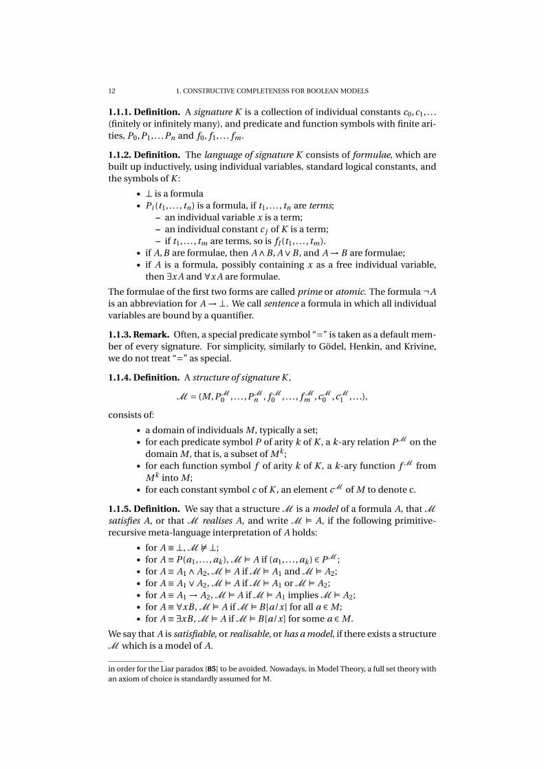
1.1.1. Definition. A signature K is a collection of individual constants c0,c1, . . .(finitely or infinitely many), and predicate and function symbols with finite ari-ties, P0,P1, . . .Pn and f0, f1, . . . fm .
1.1.2. Definition. The language of signature K consists of formulae, which arebuilt up inductively, using individual variables, standard logical constants, andthe symbols of K :
• ⊥ is a formula• Pi (t1, . . . , tn) is a formula, if t1, . . . , tn are terms;
– an individual variable x is a term;– an individual constant c j of K is a term;– if t1, . . . , tm are terms, so is fl (t1, . . . , tm).
• if A,B are formulae, then A∧B , A∨B , and A → B are formulae;• if A is a formula, possibly containing x as a free individual variable,
then ∃x A and ∀x A are formulae.
The formulae of the first two forms are called prime or atomic. The formula ¬A
is an abbreviation for A →⊥. We call sentence a formula in which all individualvariables are bound by a quantifier.
1.1.3. Remark. Often, a special predicate symbol “=” is taken as a default mem-ber of every signature. For simplicity, similarly to Gödel, Henkin, and Krivine,we do not treat “=” as special.
1.1.4. Definition. A structure of signature K ,
M = (M ,PM
0 , . . . ,PM
n , f M
0 , . . . , f M
m ,cM
0 ,cM
1 , . . .),
consists of:
• a domain of individuals M , typically a set;• for each predicate symbol P of arity k of K , a k-ary relation PM on the
domain M , that is, a subset of M k ;• for each function symbol f of arity k of K , a k-ary function f M from
M k into M ;• for each constant symbol c of K , an element cM of M to denote c.
1.1.5. Definition. We say that a structure M is a model of a formula A, that M
satisfies A, or that M realises A, and write M Í A, if the following primitive-recursive meta-language interpretation of A holds:
• for A ≡⊥, M 6Í ⊥;• for A ≡ P (a1, . . . , ak ), M Í A if (a1, . . . , ak ) ∈ PM ;• for A ≡ A1 ∧ A2, M Í A if M Í A1 and M Í A2;• for A ≡ A1 ∨ A2, M Í A if M Í A1 or M Í A2;• for A ≡ A1 → A2, M Í A if M Í A1 implies M Í A2;• for A ≡∀xB , M Í A if M Í B [a/x] for all a ∈ M ;• for A ≡∃xB , M Í A if M Í B [a/x] for some a ∈ M .
We say that A is satisfiable, or realisable, or has a model, if there exists a structureM which is a model of A.
in order for the Liar paradox [85] to be avoided. Nowadays, in Model Theory, a full set theory withan axiom of choice is standardly assumed for M.

1.1. HISTORICAL OVERVIEW 13
1.1.6. Definition. Let K be a signature. We say that a formula A, written in thelanguage of signature K , is true, or valid, if any structure M of signature K is amodel of A.
We now have set up the basic framework for looking at the major instancesof the theorem which appeared through history. In this chapter ⊢ A will standfor derivability of A inside a system for classical predicate logic. In Subsections1.1.2, 1.1.3, and 1.1.4, we assume also a classical metalanguage.
1.1.2. Gödel’s proof. We give a sketch of Gödel’s original proof, based on[84, 83, 82]. The key role is played by the following lemma, today known asModel Existence Lemma.
1.1.7. Lemma. For every formula A of a language with signature K , either there
exists a structure M of signature K such that M Í A, or ⊢¬A.
1.1.8. Theorem (Completeness). If A is true, then A is derivable.
PROOF. We apply Lemma 1.1.7 on the formula ¬A. Then, if there is a modelM of ¬A, we obtain contradiction, since M is by hypothesis also a model of A.Otherwise, the formula ¬¬A is derivable, hence A is itself derivable . �
PROOF SKETCH OF LEMMA 1.1.7. We say that a formula A is refutable if ¬A
is derivable. Gödel shows that every formula is either satisfiable or refutable,by showing that every formula in prenex normal form is either satisfiable orrefutable, since we know that the equivalence between a formula and its prenexnormal form is derivable. Actually, it is enough to consider prenex normal formswhere the left-most quantifier is universal, because each prefixing existentialquantifier can be immediately eliminated by replacing the variable it binds witha constant. Let the degree of such a prenex normal formula be the number ofblocks of universal quantifiers separated by existential ones. The proof is by in-duction on the degree:
(1) If every formula of degree k is either satisfiable or refutable, then so is
every formula of degree k + 1. This is proved by Skolemisation. A for-mula of degree k +1 is transformed into one of degree k which is equi-satisfiable with the first one. New function symbols are introduced inthe process.
(2) Every formula of degree 1 is either satisfiable or refutable. A formula P
of degree 1 is of the form ∀~r∃~n A(~r ;~n), where ~r denotes a q-tuple ofvariables, and ~n denotes an s-tuple of variables. Let (~rn) be an infinitesequence of q-tuples of variables x0, x1, x2 . . . generated in (some) lexi-cographical order:
~r1 = (x0, x0, . . . , x0)
~r2 = (x1, x0, . . . , x0)
~r3 = (x0, x1, . . . , x0)
...

14 1. CONSTRUCTIVE COMPLETENESS FOR BOOLEAN MODELS
We define the sequence of formulae An by
A1 = A(~r1; x1, x2, . . . xs)
A2 = A(~r2; x1+s , x2+s , . . . x2s)∧ A1
...
An = A(~rn ; x(n−1)s+1, x(n−1)s+2, . . . xns)∧ An−1
...
where, for each An , the variables put in the places bound by the exis-tential quantifier do not appear in the formulae Am for m < n. We de-note by Pn the formula ∃x0 · · ·∃xns An . It is easy to show that P ⇒ Pn isderivable. Now, because each of An is a formula of propositional logic,(a) either some An is refutable, and hence P is refutable because Pn is
refutable;(b) or, no An is refutable, that is, all An are satisfiable, and hence we
get an infinite sequence of models
M1 ⊆M2 ⊆ ·· · ⊆Mn ⊆ ·· · .
Then M :=∪i∈NMi is a model of the formula P .
�
The introduction notes to [82, 83, 84] see in the last step an applicationof Konig’s lemma, although Gödel himself justifies the step by “familiar argu-ments”.
1.1.3. Henkin’s proof. It was Henkin who apparently first remarked the slightimprecision in the Skolemisation step of Gödel’s proof. Namely, in order to elim-inate existential quantifiers that follow universal ones, Skolemisation introducesnew function symbols which are not interpreted in the models M1 ⊆ M2 ⊆ ·· · ,because they come from an extended language.
It is Henkin’s proof which is standard in today’s textbooks on logic. It wascarried out in his PhD thesis and published in article form as [94]. Henkin’s the-sis goes beyond the article [94], because it also discusses completeness in thecontext of higher-order logic and proves, using completeness, Stone’s represen-tation theorem for Boolean algebras.
The key role is played by the following Model Existence Lemma.
1.1.9. Lemma. Let S0 be a signature. If Λ is a set of sentences of signature S0,
which is consistent (Λ 6⊢ ⊥), then Λ has a model.
PROOF SKETCH. Let Si+1 be a signature that extends Si with countably manynew constant symbols ui+1
0 ,ui+11 , . . .. A set of sentences Γ of signature S will be
called maximal consistent if, for any sentence A of signature S, A 6∈ Γ→ Γ, A ⊢
⊥ & Γ 6⊢ ⊥, that is, if (Γ, A ⊢⊥→ Γ⊢⊥) implies A ∈ Γ.We will now construct Γ0, a maximal consistent set of sentences of S0, that
contains the given set Λ. Let Γ0,0 := Λ. We fix an enumeration of formulae ofsignature S0. Let Γ0,1 := Γ0,0 ∪ {B1}, where B1 is the first formula from the enu-meration such that Γ0,0 ∪ {B1} is consistent. In general, let Γ0,i+1 := Γ0,i ∪ {Bi+1},where Bi+1 is the (i +1)-th formula from the enumeration such that Γ0,i ∪ {Bi+1}is consistent. We set Γ0 :=∪i∈NΓ0,i , for which we have that:
1.1. HISTORICAL OVERVIEW 15
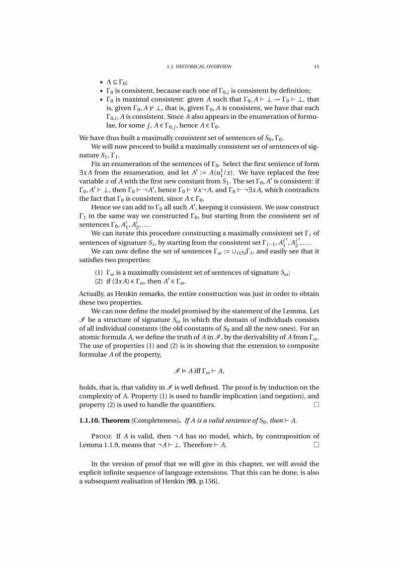
• Λ⊆ Γ0;• Γ0 is consistent, because each one of Γ0,i is consistent by definition;• Γ0 is maximal consistent: given A such that Γ0, A ⊢ ⊥ → Γ0 ⊢ ⊥, that
is, given Γ0, A 6⊢ ⊥, that is, given Γ0, A is consistent, we have that eachΓ0,i , A is consistent. Since A also appears in the enumeration of formu-lae, for some j , A ∈ Γ0, j , hence A ∈ Γ0.
We have thus built a maximally consistent set of sentences of S0, Γ0.We will now proceed to build a maximally consistent set of sentences of sig-
nature S1, Γ1.Fix an enumeration of the sentences of Γ0. Select the first sentence of form
∃x A from the enumeration, and let A′ := A{u11/x}. We have replaced the free
variable x of A with the first new constant from S1. The set Γ0, A′ is consistent: ifΓ0, A′ ⊢⊥, then Γ0 ⊢ ¬A′, hence Γ0 ⊢ ∀x¬A, and Γ0 ⊢ ¬∃x A, which contradictsthe fact that Γ0 is consistent, since A ∈ Γ0.
Hence we can add to Γ0 all such A′, keeping it consistent. We now constructΓ1 in the same way we constructed Γ0, but starting from the consistent set ofsentences Γ0, A′
1, A′2, . . . .
We can iterate this procedure constructing a maximally consistent set Γi ofsentences of signature Si , by starting from the consistent set Γi−1, Ai
1′, Ai
2′, . . ..
We can now define the set of sentences Γω := ∪i∈NΓi , and easily see that itsatisfies two properties:
(1) Γω is a maximally consistent set of sentences of signature Sω;(2) if (∃x A) ∈ Γω, then A′ ∈ Γω.
Actually, as Henkin remarks, the entire construction was just in order to obtainthese two properties.
We can now define the model promised by the statement of the Lemma. LetI be a structure of signature Sω in which the domain of individuals consistsof all individual constants (the old constants of S0 and all the new ones). For anatomic formula A, we define the truth of A in I , by the derivability of A from Γω.The use of properties (1) and (2) is in showing that the extension to compositeformulae A of the property,
I Í A iff Γω ⊢ A,
holds, that is, that validity in I is well defined. The proof is by induction on thecomplexity of A. Property (1) is used to handle implication (and negation), andproperty (2) is used to handle the quantifiers. �
1.1.10. Theorem (Completeness). If A is a valid sentence of S0, then ⊢ A.
PROOF. If A is valid, then ¬A has no model, which, by contraposition ofLemma 1.1.9, means that ¬A ⊢⊥. Therefore ⊢ A. �
In the version of proof that we will give in this chapter, we will avoid theexplicit infinite sequence of language extensions. That this can be done, is alsoa subsequent realisation of Henkin [95, p.156].

16 1. CONSTRUCTIVE COMPLETENESS FOR BOOLEAN MODELS
1.1.4. Krivine’s proof. Krivine was the first to give a constructive proof [125]of Gödel’s completeness theorem.2 He shows that the statement of complete-ness for first-order logic can be formalised as a true formula TC of classical second-order logic, with the axiom schema of comprehension and the axiom of fullsecond-order induction. The formula TC uses five function symbols {0, s, ,→,σ,@}, but no axioms are supposed for the last three of those.
A concrete proof of completeness of first-order logic can be obtained by build-ing a concrete second-order model M0, which interprets the five function sym-bols in the intended way:
• the domain of individuals of M0 is the set of first-order sentences ofa signature L which, besides the five function symbols, contains alsocountably many constant symbols;
• for a fixed enumeration of the sentences, the nullary function symbol 0is interpreted as the first formula in the enumeration, and s is a unaryfunction symbol that, given a formula, returns the next one accordingto the enumeration;
• the binary function symbol ,→ is interpreted as implication betweensentences;
• for a fixed bijection G 7→ tG between sentences and closed terms of sig-nature L, the function symbol σ is interpreted as substitution:
σ(∀x A′,B) := A′{tB /x},
σ(A,B) := A, if A is not a universal formula.
and @ is interpreted as a generator of fresh terms:
@(A,B) := tC
where C is a sentence such that the term tC does not appear in A andB .
• the second order variables of arity n are interpreted, as usually for second-order models, by n-ary relations on the domain of M0.
Krivine’s proof is constructive because the formula TC has a form such thatits double-negation translation is equivalent to TC inside intuitionistic second-order logic.
Since the article [125] contains a very detailed formal argument, we will herecontent ourselves to just describing the formula TC and giving a sketch of theproof.
Let M and J be unary second-order variables. In the model M0, such anentity is a collection of formulae. Let ∀x Ent(x) denote the axiom of second-order induction, that is, let Ent(x) be the formula:
∀X(∀y
(X y → X (s y)
)→ X 0 → X x
).
2N.B. Observations that Gödel’s proof is essentially constructive appear already, in a coupleof places, in the papers [119, 116, 120] of Kreisel.

1.1. HISTORICAL OVERVIEW 17
We define the predicate Mod(M), to be read as “M is a model”, by the conjunc-tion of the following formulae:
∀x y(M(x ,→ y) → M x → M y
)
∀x y(Ent(x) → (M x → M y) → M(x ,→ y)
)
∀x y(M x → M(σ(x, y))
)
∀x(Ent(x) → (∀y M(σ(x, y))) → M x
)
We also define a predicate Ded(J ), to be read as “J is closed by deduction”, by theconjunction of the following formulae, which, in the model M0, express that J isa collection of formulae closed under deduction from the rules of Hilbert’s sys-tem for propositional calculus plus the axioms for introduction and eliminationof the universal quantifier.
∀x y J (y ,→ x ,→ y)
∀x y z J ((x ,→ y) ,→ (x ,→ y ,→ z) ,→ x ,→ z)
∀x y J (((x ,→ y) ,→ x) ,→ x) Peirce’s law
∀x y J (x ,→ y) → J x → J y modus ponens
∀x y J (x ,→σ(x, y))
∀x y J((σ
(x,@
(x, y
)),→ y
),→ y
)→ J
((x ,→ y
),→ y
)
Now, starting from the simple version of completeness specified by the for-mula
(TC0) ∀x (∀M (Mod(M) → M x) →∀J (Ded(J ) → J x)) ,
we generalise to the full statement of completeness, where the formula x is validand derivable modulo a collection of formulae P (that is, a collection of axioms),
(TC0(P )) ∀x (∀M (Mod(M) → P ⊆ M → M x) →∀J (Ded(J ) → P ⊆ J → J x)) ,
and we finally arrive at
(TC) ∀x∀J (∀M (Mod(M) → J ⊆ M → M x) → Ded(J ) → J x)
which is equivalent to ∀P.TC0(P ).
1.1.11. Theorem. The formula TC is a valid formula of both intuitionistic and of
classical second-order logic, with as axioms the comprehension schema and full
second-order induction, in the language {0, s, ,→,σ,@}.
PROOF SKETCH. The proof is carried out in classical second-order logic, andis afterwards translated by a double-negation interpretation into intuitionisticsecond-order logic.
Although the full proof from [125] works independently of interpretation,this sketch works in the intended model M0.
Let G0,G1, . . . be an enumeration of sentences, and let a be a given sentence.We define by recursion a sequence of sentences φ0,φ1, . . . by:
φ0 := a
φn+1 :=φn if (Gn ,→φn) ,→φn ∈ J
φn+1 := (G ′n{c/x} ,→φn) ,→φn otherwise, if Gn is of form ∀xG ′
n
φn+1 := (Gn ,→φn) ,→φn otherwise

18 1. CONSTRUCTIVE COMPLETENESS FOR BOOLEAN MODELS
where c is a constant symbol not appearing in φn ,Gn . Now, define
M := {φ | ∃n.((φ ,→φn) ,→φn) ∈ J }.
It rests to show that Mod(M) and a 6∈ M . �
In his article, Krivine also attempts to solve the “specification problem” forTC, that is, to determine the common operational behaviour of all different pro-grams that correspond to proofs of TC. He claims that the specification of TCis the one of an “interactive disassembler equipped with protection for systemcalls”.
1.1.5. The proof of Berardi and Valentini. Berardi and Valentini “reverseengineered” Krivine’s proof into a more conventional and less formal one, at thesame time isolating what they see as the main principle behind, a constructiveversion of the Ultra-filter Theorem for countable Boolean algebras.
Krivine uses a notion of truth which is not the standard one, namely, thereis no requirement that ⊥ be not true in a model. This, as he himself remarks,means that, classically, there is exactly one model which is not a standard Tarskimodel, the all-true model. Additionally, Berardi and Valentini remark that, dueto a result of McCarthy [135], if completeness of classical predicate logic with re-spect to standard Tarski models was provable intuitionistically, then there wouldbe an intuitionistic proof of Markov’s Principle; however, Markov’s Principle isindependent of intuitionistic logic (Heyting Arithmetic) [119].
A similar phenomenon happens with intuitionistic completeness of intu-itionistic logic (that will be treated in Chapter 3): in order to avoid the meta-mathematical results of Gödel and Kreisel [120], Veldman [175] has to give spe-cial treatment to ⊥ in the semantics by allowing “exploding” nodes that can val-idate ⊥.
1.1.12. Definition. A minimal model is a set of sentences M which is:
• implication-faithful: A ⇒ B ∈ M ↔ (A ∈ M → B ∈ M);• for-all-faithful: for every formula A with at most one free variable x,∀x.A(x) ∈ M ↔ for any closed term t , A(t ) ∈ M ;
• meta-DN : (¬A ∈ M →⊥∈ M) → A ∈ M
1.1.13. Definition. A standard model is a minimal model M with the additionalproperty that ⊥ 6∈ M .
1.1.14. Remark. For any standard model M there corresponds a model M inthe sense of Definition 1.1.5, and vice versa. What we call “standard model” isknown as “the theory” of a Tarski model, that is the set of all sentences true inthe Tarski model.
In [29], Berardi and Valentini prove in detail their constructive version of theUltra-filter theorem, and outline how a Henkin-style proof based on it shouldlook like. In the following sections we give a detailed proof of both the Ultra-filter Theorem and the completeness theorem, generalising slightly the Ultra-filter Theorem to setoids (sets equipped with an equality relation which is notnecessarily substitutive).

1.2. CONSTRUCTIVE ULTRA-FILTER THEOREM 19
1.2. Constructive ultra-filter theorem
1.2.1. Definition. A Countable Boolean Algebra over a setoid (B ,=), B, consistsof an interpretation of the constants {∧,∨,⊥,⊤,¬,p·q} which satisfies the follow-ing axioms.
x∧x=x (x∨y)∧z=(x∧z)∨(x∧z)
x∨x=x (x∧y)∨z=(x∨z)∧(x∨z)
x∧y=y∧x ⊥∧x=⊥
x∨y=y∨x ⊥∨x=x
x∧(y∧z)=(z∧y)∧z ⊤∧x=x
x∨(y∨z)=(z∨y)∨z ⊤∨x=⊤
x∧(x∨y)=x x∧¬x=⊥
x∨(x∧y)=x x∨¬x=⊤
pxq= pyq→ x = y
1.2.2. Fact. The following defines a partial order on B:
x≤y := (x∧y)=x.
We will now need to talk about a collection F of elements of B . Although wethink of it as a predicate over B , we will use the notation F ⊆ B and say that F isa subset. We will denote interchangeably by F x and x ∈ F membership in F. Nouse of a power-set axiom is made.
1.2.3. Definition. A subset F ⊆ B is called a filter if it is:
• inhabited: ∃x : B ,F x
• upwards closed: ∀x y : B ,F x → x≤y → F y
• meet-closed: ∀x y : B ,F x → F y → F (x∧y)
1.2.4. Definition. If X ⊆ B , the closure of X , ↑X , is the set of all elements of B
which are greater than some finite meet of elements of X i.e.
↑X :=λb.∃y1, . . . , yn ∈ X . y1∧ · · · ∧yn≤b
1.2.5. Definition. X ⊆ F is inconsistent if X ⊥, and X ,Y ⊆ B are equiconsistent
(X ∼ Y ) if X ⊥↔ Y ⊥.
1.2.6. Definition. X ⊆ B is element-complete for b ∈ B if
(X ∼↑(X ∪ {b})) → b ∈ X .
X is complete if it is element-complete for all b ∈ B .
1.2.7. Remark. Note that this definition of “complete”, classically equivalent tothe more usual one (for all b, either b ∈ F or ¬b ∈ F ), is key to having a construc-tive proof of the Ultra-filter Theorem.
1.2.8. Fact. We list without proof some easy properties of filters. These areproved in the Coq formalisation.
(1) For every X ⊆ B , the closure ↑X is a filter.(2) If F is a filter, then ⊤ ∈ F .(3) For any X ⊆ B , X ⊆↑X .

20 1. CONSTRUCTIVE COMPLETENESS FOR BOOLEAN MODELS
(4) If X ⊆ Y ⊆ B , then ↑X ⊆↑Y .(5) If F is a filter, then F =↑F .
1.2.9. Proposition. If F ⊆ B is a filter, then x=y and x ∈ F imply y ∈ F .
PROOF. Immediate from F being upwards closed. �
We will need the following definition and properties for the proof of theUltra-filter Theorem.
1.2.10. Definition. Let F be a filter. Using the enumeration p·q : B → N, definethe primitive-recursive fixed point Fn ⊆ B by
F0 := F
Fn+1 :=λb. ↑(Fnb ∨ (pbq= n ∧Fn ∼↑(Fn ∪ {b}))) .
1.2.11. Lemma. For every n, Fn is a filter.
PROOF. A simple induction on n using Fact 1.2.8(1). �
1.2.12. Lemma. If n ≤ m, then Fn ⊆ Fm .
PROOF. By induction on the generation of the relation ≤ (because ≤ has aninductive definition), and using Fact 1.2.8(1). �
1.2.13. Lemma. For every n, F0 ∼ Fn . For every n,m, Fn ∼ Fm . For any k, and Z
as defined in the next theorem, Z ∼ Fk .
PROOF. By induction on n, we prove the first part, the other two are easyconsequences of it.
The base case is immediate. Let F ∼ Fn and let ⊥ ∈ Fn+1. We have to provethat ⊥ ∈ F . By definition, ⊥ ∈ Fn+1 means that
∃y1, . . . , yl ∈ {Fn ∪ {b | pbq= n ∧Fn ∼↑(Fn ∪ {b})}} . y1∧ · · · ∧yl ≤⊥.
Now, either all of yi belong to Fn , in which case ⊥ ∈ Fn ∼ F ; or, some of themare equal to a b such that pbq= n, but, in that case, ⊥ ∈↑(Fn ∪ {b}) ∼ Fn ∼ F . �
1.2.14. Theorem. If F is a filter, then Z := λb.∃n.Fnb = ∪n∈NFn is a complete
filter extending F , that is equiconsistent with F .
PROOF. Z is a filter: it is inhabited because F0 is inhabited, it is upwardsclosed because each one of Fn is (Lemma 1.2.11), and Z is meet-closed becauseof Lemma 1.2.12.
Z ∼ F because of Lemma 1.2.13.To show that Z is complete, let x : B with Z ∼↑(Z ∪ {x}) be given. We show
that x ∈ Z , by showing that Fn ∼↑(Fn ∪ {x}), when n = pxq. Direction Fn⊥ →↑
(Fn ∪ {x})⊥ follows from Fact 1.2.8(3). Let ↑(Fn ∪ {x})⊥. Then ↑(Z ∪ {x})⊥, byFact 1.2.8(4). By equiconsistency with Z , we have Z ⊥. By Lemma 1.2.13, we getFn⊥. �
The theorem we just proved is the one that is used for proving the complete-ness theorem of the next section. We now proceed to give a more familiar formof the Ultra-filter Theorem as a corollary.
1.2.15. Definition. A filter H is an ultra-filter if, whenever G is a filter such thatH ∼G and H ⊆G , then also G ⊆ H .

1.3. CONSTRUCTIVE HENKIN-STYLE PROOF 21
1.2.16. Corollary. For any starting filter F , Z (F ) is an ultra-filter.
In particular, if F is consistent (⊥ 6∈ F ), we get a proof of a standard formula-
tion of the Ultra-filter Theorem.
PROOF. Let G be a filter such that Z (F ) ⊆ G and Z (F ) ∼ G . To prove thatG ⊆ Z (F ), let a ∈ G and use the completeness of Z (F ). We have to show thatZ (F ) ∼↑(Z (F )∪ {a}). One direction is obvious, for the other, let ⊥ ∈↑(Z (F )∪ {a}).From the hypotheses and Fact 1.2.8, we get that ⊥ ∈↑G =G ∼ Z (F ). �
1.3. Constructive Henkin-style proof
We now proceed to the constructive completeness proof à la Henkin. Themain difference with other such proofs is that we do not build an infinite ex-tension of signatures S0,S1, . . . explicitly, as Henkin does, but instead extend thegrammar of formulae with a separate class of constants, Henkin constants. Inthe end, when completeness is stated, we require that the input formula con-tains no Henkin constants, hence the completeness theorem works only for stan-dard formulae.
1.3.1. Definition. The extended language of signature K consists of extended for-
mulae, which are built up inductively, using individual variables, standard logi-cal constants, the symbols of K , and a special constant symbol cA for each for-mula A:
• ⊥ is a formula• Pi (t1, . . . , tn) is a formula, if t1, . . . , tn are terms;
– an individual variable x is a term;– an individual constant c j of K is a term;– a Henkin constant cA , for A-formula, is a term;– if t1, . . . , tm are terms, so is fl (t1, . . . , tm).
• if A,B are formulae, then A∧B , A∨B , and A → B are formulae;• if A is a formula, possibly containing x as a free individual variable,
then ∃x A and ∀x A are formulae.
In other words, the extended formulae are built from three kinds of expressions:formulae can be constructed from terms, terms can be constructed from con-stants, and constants can be constructed from formulae.
For a derivation system we take the one of Table 1.
A ∈ ΓAX
Γ⊢ A
Γ, A1 ⊢ A2 ⇒IΓ⊢ A1 ⇒ A2
Γ⊢ A1 ⇒ A2 Γ⊢ A1 ⇒EΓ⊢ A2
Γ⊢ A x-fresh∀I
Γ⊢∀x AΓ⊢∀x A
∀EΓ⊢ A{t/x}
Γ⊢⊥⊥E
Γ⊢ AΓ⊢ (A ⇒⊥) ⇒⊥
¬¬EΓ⊢ A
Table 1: Classical natural deduction with {⇒,∀,⊥}

22 1. CONSTRUCTIVE COMPLETENESS FOR BOOLEAN MODELS
1.3.2. Fact. Given a derivation Γ ⊢ A, we can replace a constant c with a freshvariable x, obtaining a derivation Γ{x/c} ⊢ A{x/c}.
The proof of this fact is very technical, but since it is well known and we didprove it formally in Coq, we leave it out.
1.3.3. Definition. Given a set of sentences (axioms) A , the theory of A , Th(A ),is the set of formulae which are derivable from the axioms.
1.3.4. Definition. The set of Henkin-axioms H is the set of formulae of formA(c∀x A) ⇒∀x A for A such that ∀x A is closed.
1.3.5. Definition. A set of formulae T is Henkin-complete if H ⊆T .
1.3.6. Lemma. If A is a set of sentences (axioms) which contains no Henkin con-
stants, then the theories Th(A ∪H ) and Th(A ) are equiconsistent.
PROOF. That ⊥ ∈ Th(A ) →⊥ ∈ Th(A ∪H ) is clear. Let ⊥ ∈ Th(A ∪H ) i.e.Γ ⊢ ⊥ for some Γ ∈ A ∪H . We show that we can eliminate all Henkin axiomsfrom Γ, by showing that we can eliminate one at a time, when the Henkin con-stant the axiom is based on does not appear in the other formulae of the context.Once we show that, we just need to reorder3 the Henkin axioms from Γ so thatthe most complex ones are eliminated first.
Let (A(c∀x A) ⇒∀x A),∆⊢⊥, where the constant c∀x A does not appear in ∆.We want to show ∆⊢⊥. It will be enough to show that ∆⊢ ∀y¬(A ⇒∀x A), be-cause this produces a contradiction with a tautology of classical predicate logic,the Drinker paradox:4
⊢¬∀y¬(A ⇒∀x A)
Let y be a fresh variable. We need to show that ∆ ⊢ ¬(A ⇒ ∀x A)(y). Since∀x A is closed, we can rewrite the hypothesis (A(c∀x A) ⇒ ∀x A),∆ ⊢ ⊥ as ∆ ⊢
¬(A ⇒∀x A)(c∀x A). Now, since c∀x A does not appear in ∆, it is enough to applyFact 1.3.2. �
1.3.7. Definition. The Lindenbaum Boolean algebra {B,=,∧,∨,⊥,⊤,¬,p·q} is de-fined by:
B is the set of closed formulae
A1=A2 iff ⊢ A1 ⇒ A2 and ⊢ A2 ⇒ A1
A1∧A2 :=¬(A1 ⇒¬A2)
A1∨A2 :=¬A1 ⇒ A2
⊥ :=⊥
⊤ :=⊥⇒⊥
¬A :=¬A
The enumeration p·q is defined via the Cantor pairing function in Section 1.5.2.
1.3.8. Lemma. Every theory is a filter in the Lindenbaum Boolean algebra.
PROOF. This is easy to show. For details have a look at the formal proof. �
3Actually, the correctness of the reordering(sorting) algorithm is the only part of the proofwhich was not fully formalised in Coq. See Section 1.5 for more details.
4Which can be phrased in natural language by: “There is someone in the pub such that, if heis drinking, everyone in the pub is drinking”.

1.3. CONSTRUCTIVE HENKIN-STYLE PROOF 23
Let Fn be defined by setting F0 := Th(A ∪H ) in the fixpoint of Defini-tion 1.2.10, and let Z be defined, like in Theorem 1.2.14, as B ∈Z ↔∃n.B ∈Fn .
1.3.9. Lemma. For every n, the filter Fn is the theory with axiom set Gn , where
G0 :=A ∪H
Gn+1 :=λb. (Gnb ∨ (pbq= n ∧Fn ∼↑(Fn ∪ {b}))) .
The complete filter Z is the theory with axiom set ∪n∈NGn .
PROOF. Direction “→” of the first part is by induction on n. F0 is a theoryby definition. Let Fn = Th(Gn) and A ∈ Fn+1. We have to show that there is aderivation Γ⊢ A such that Γ⊆Gn+1. By the definition of the fixpoint,
A ∈↑(Fn ∪ {b | pbq= n & Fn ∼↑(Fn ∪ {b})}) ,
that is,
∃y1, . . . , ym ∈Fn ∪ {b | pbq= n & Fn ∼↑(Fn ∪ {b})} . y1∧ · · · ∧ym≤A,
and, by the induction hypothesis,
∃z11 , . . . , z
k11 , z1
2 , . . . , zk22 , . . . , z1
m , . . . , zkmm ∈Gn+1. z1
1∧ · · · ∧zkmm ≤A,
from which the goal follows by the interpretation of ∧ and ≤ in the Lindenbaumalgebra.
Direction “←” is immediate because Gn ⊆Fn for every n.The statement Z ⊆ Th(∪n∈NGn) follows directly from the first part.To show Th(∪n∈NGn) ⊆Z , let Γ⊢ A and Γ⊆∪n∈NGn . Note that Γ⊆∪n∈NGn
is just a shortcut for ∀x A ∈ Γ, A ∈ ∪n∈NGn . To show that A ∈ Z means to find m
such that A ∈ Fm . We simply need to take for m the maximum n such that allformulae of Γ belong to Fn (by Lemma 1.2.12). Now, from Γ⊢ A, we have
∧Γ≤A,
therefore, since Fm is a filter, A ∈Z .�
We are now ready to prove the main theorem.
1.3.10. Theorem (Model Existence). Let A be a set of axioms that does not con-
tain any Henkin constants. Then Z is an equiconsistent extension of Th(A ) that
is implication-faithful, for-all-faithful, and meta-DN.
PROOF. That Z is an equiconsistent extension of Th(A ) follows from Lemma1.3.6 and Theorem 1.2.14. We need to show that Z is a minimal model.
• Z is meta-DN. Let A be a sentence such that ¬A ∈Z →⊥∈Z . We needto show that A ∈Z . We will use the fact that Z is complete, that is,
Z ∼↑(Z ∪ {A}) → A ∈ Z .
The direction “→” of Z ∼↑(Z ∪ {A}) is trivial. Let ⊥ ∈↑(Z ∪ {A}). Weshow that ⊥ ∈ Z by applying the first hypothesis, but then we have toshow that ¬A ∈Z . By the definition of ↑ we have that
∃y1, y2, . . . , ym ∈Z ∪ {A}.y1∧y2∧ · · · ∧ym≤⊥.
Now, we look at two cases:(1) Either all yi are in Z , and then, by Z being a filter, ¬A ∈ Z , be-
causey1∧y2∧ · · · ∧ym≤⊥≤¬A.

24 1. CONSTRUCTIVE COMPLETENESS FOR BOOLEAN MODELS
(2) Or, yρ(1), yρ(2), . . . , yρ(m−1) ∈Z and yρ(m) = A, and then, since
yρ(1)∧yρ(2)∧ · · · ∧yρ(m−1)∧A≤⊥,
we have that
yρ(1)∧yρ(2)∧ · · · ∧yρ(m−1) ≤¬A.
Since Z is a filter, ¬A ∈Z .• Z is implication-faithful. We have to show that
(A ⇒ B) ∈Z ↔ (A ∈Z → B ∈Z ).
Direction “→” follows directly by the ⇒E rule, because Z is a theory byLemma 1.3.9.
Let A ∈ Z → B ∈ Z . We show (A ⇒ B) ∈ Z by applying the fact weproved above, that Z is meta-DN, hence we have to show that
¬(A ⇒ B) ∈Z →⊥∈Z .
Let ¬(A ⇒ B) ∈ Z . Since Z is a (classical) theory, we have that A ∈ Z
and ¬B ∈Z . Now, from the hypothesis and A ∈Z we get B ∈Z , hence⊥∈Z .
• Z is for-all-faithful. We have to show that, for any formula A such that∀x A is closed,
(∀x A) ∈Z ↔ for any closed term t , A{t/x} ∈Z .
Direction “→” is by the ∀E rule, because Z is a theory.Let for any closed term t , A(t ) ∈ Z . By definition, Z is Henkin-
complete. Then, we can show that ∀x A ∈ Z by using implication-fatefulness on the Henkin axiom,
A(c∀x A) ⇒∀x A,
because from the hypothesis we can conclude that A(c∀x A) ∈Z .
�
Let Γ Í A denote that, for every minimal model M , Γ ⊆ M implies A ∈ M .We have the following corollary.
1.3.11. Corollary (Completeness). For any Γ and A that do not contain Henkin
constants, if ΓÍ A, then Γ⊢ A.
PROOF. Let the set of axioms C be the finite set Γ∪{¬A}. By Theorem 1.3.10,there is a minimal model M := Z (C ) that extends Th(C ) and is equiconsistentwith it. Because A is true in any model in which Γ is true, and because Γ ⊆
Th(C ) ⊆ M , we have that A ∈ M . But, because also ¬A ∈ Th(C ) ⊆ M , we getthat ⊥ ∈ M . Since M and Th(C ) are equiconsistent, also ⊥ ∈ Th(C ), which, bydefinition, means that Γ,¬A ⊢⊥. Hence, Γ⊢ A. �
1.4. Computational content
The computational content of the completeness proof is to be read off Theo-rem 1.3.10. We do not give a succinct characterisation of it like the one of Krivine,mentioned at end of section 1.1.4, but instead discuss multiple aspect.
Theorem 1.3.10 builds the model Z using a fixed-point, starting from Th(A∪
H ). The built model Z is equiconsistent with Th(A ), so the Henkin axioms

1.5. ASPECTS OF THE COQ FORMALISATION 25
somehow “disappear”. The procedure behind this is described in the proof ofLemma 1.3.6: we take a derivation Γ⊢ A that uses Henkin axioms, we order theaxioms according to the depth of the formula which is annotating the Henkinconstant, and then we eliminate them one by one by using the Drinker’s paradoxand Fact 1.3.2, which replaces all occurrences of a constant inside a derivationby a free variable.
Let us now pose the question: how does Theorem 1.3.10 “normalise” proofsinvolving implication, that is, what is the procedure to construct a derivationΓ⊢ B from derivations ofΓ⊢ A ⇒ B andΓ⊢ A. When we think of calculi that sat-isfy the Brouwer-Heyting-Kolmogorov interpretation [161, p.10] of logical con-nectives, we think of this proof transformation as the β-reduction relation onproof terms.
The statement A ⇒ B ∈ Z determines an “approximation” of Z , a numbern such that A ⇒ B ∈ Fn , and A ∈ Z determines a number m such that A ∈ Fm .Then, the proof that Z is a theory from Lemma 1.3.9, shows the way to provethat B ∈ Z : we take the common approximation of Z of all formulae used in aderivation of B , and return that number. In the simplest case we have above, wereturn max(n,m).
In the next chapters we will refer to the statement
(A ⇒ B) ∈Z → A ∈Z → B ∈Z
as reflection. The converse,
(A ∈Z → B ∈Z ) → (A ⇒ B) ∈Z ,
will be referred to as reification. In Theorem 1.3.10, reification is proved via themeta-DN property of Z ,
for any formula C , (¬C ∈Z →⊥∈Z ) →C ∈Z .
Using reflection, we can transform this to
for any formula C , ((C ∈Z →⊥∈Z ) →⊥∈Z ) →C ∈Z ,
from which we see that meta-DN transforms a higher-order proof, written in akind of continuation-passing style [143], into a flat classical proof.
1.5. Aspects of the Coq formalisation
The source code of the formalisation is available at the address ❤tt♣✿✴✴
✇✇✇✳❧✐①✳♣♦❧②t❡❝❤♥✐q✉❡✳❢r✴⑦❞❛♥❦♦✴❝♦❞❡.As we mentioned in the introduction, the formalisation is not complete. The
missing part is the correctness of the sorting algorithm needed in Lemma 1.3.6.The reason why this part remained unfinished is that in the formal proof of thelemma, we used a sorting specification which was convenient for the proof, butwas an ad hoc specification as far as general list sorting is concerned, thus wecould not reuse the already proven results about general list sorting in Coq. Forlack of time, we contented ourselves by testing in Coq that the sorting algorithmcomputes as expected.

26 1. CONSTRUCTIVE COMPLETENESS FOR BOOLEAN MODELS
1.5.1. Formal syntax of formulae and co-finite rule for ∀I . The syntax offormulae is defined using the following inductive datatype.
P❛r❛♠❡t❡rs ❢✉♥❝t✐♦♥ ♣r❡❞✐❝❛t❡ ❝♦♥st❛♥t✵ : ❙❡t.
■♥❞✉❝t✐✈❡ ❢♦r♠✉❧❛ : ❙❡t :=| ❜♦t : ❢♦r♠✉❧❛
| ✐♠♣ : ❢♦r♠✉❧❛→ ❢♦r♠✉❧❛→ ❢♦r♠✉❧❛
| ❛❧❧ : ❢♦r♠✉❧❛→ ❢♦r♠✉❧❛
| ❛t♦♠ : ♣r❡❞✐❝❛t❡ → t❡r♠→ ❢♦r♠✉❧❛
✇✐t❤ t❡r♠ : ❙❡t :=| ❜✈❛r : ♥❛t→ t❡r♠
| ❢✈❛r : ♥❛t→ t❡r♠
| ❝♥st : ❝♦♥st❛♥t→ t❡r♠
| ❢✉♥❝ : ❢✉♥❝t✐♦♥ → t❡r♠→ t❡r♠
✇✐t❤ ❝♦♥st❛♥t : ❙❡t :=| ♦r✐❣✐♥❛❧ : ❝♦♥st❛♥t✵ → ❝♦♥st❛♥t
| ❛❞❞❡❞ : ❢♦r♠✉❧❛→ ❝♦♥st❛♥t.
One thing to notice is that we have a truly mutually inductive data-type, theclause for constants depending on the one for formulae, because of Henkin con-stants (the ones with marker ❛❞❞❡❞).
Another thing to notice is that the predicate and function constructors, ❛t♦♠and ❢✉♥❝, take only a single term as an argument. For the completeness proofto be practically useful in Coq, however, an extension to multi-argument con-structors would be necessary. Our goal has been a more theoretical one, to seethe details and computational contents of a formal type-theoretic completenessproof.
A third thing to comment about is the formal handling of variables. This isan often neglected aspect of informal proofs, but quite an important one whenformalisation is concerned. In the theory of programming languages there is acommunity effort in progress, for definite settling on good formalisation prac-tises connected to variable binding, known as the POPLMark challenge [183].Following one of the most successful approaches to binders, the “locally name-less” representation [18], we represent bound variables and free variables sepa-rately, via two separate constructors, ❜✈❛r and ❢✈❛r. ❜✈❛r-s range over numbers,deBruijn indices, while ❢✈❛r-s can range over any set with decidable equality, forexample the set of character strings. Thus, formally, a formula ∀x∀y(P (x) ⇒Q(x)) is represented by ❛❧❧ ✭✐♠♣ ✭P ✭❜✈❛r ✵✮✮ ✭◗ ✭❜✈❛r ✶✮✮✮, and a for-mula ∀x(P (x) ⇒∀yQ(y)) is represented by ❛❧❧ ✭✐♠♣ ✭P ✭❜✈❛r ✵✮✮ ✭❛❧❧ ✭◗
✭❜✈❛r ✵✮✮✮✮. Substitutions are defined via the following fixpoint.
❋✐①♣♦✐♥t
♦♣❡♥ r❡❝ (k : ♥❛t) (u : t❡r♠) (t : ❢♦r♠✉❧❛) {str✉❝t t} : ❢♦r♠✉❧❛ :=♠❛t❝❤ t ✇✐t❤
| ❜♦t⇒ ❜♦t| ✐♠♣ t1 t2 ⇒ ✐♠♣ (♦♣❡♥ r❡❝ k u t1) (♦♣❡♥ r❡❝ k u t2)| ❛❧❧ t1 ⇒ ❛❧❧ (♦♣❡♥ r❡❝ (❙ k) u t1)| ❛t♦♠ p t1 ⇒ ❛t♦♠ p (♦♣❡♥ r❡❝ t❡r♠ k u t1)
❡♥❞
✇✐t❤

1.5. ASPECTS OF THE COQ FORMALISATION 27
♦♣❡♥ r❡❝ t❡r♠ (k : ♥❛t) (u : t❡r♠) (t : t❡r♠) {str✉❝t t} : t❡r♠ :=♠❛t❝❤ t ✇✐t❤
| ❜✈❛r i ⇒ ✐❢ ❜❡q ♥❛t k i t❤❡♥ u ❡❧s❡ (❜✈❛r i)| ❢✈❛r x ⇒ ❢✈❛r x
| ❝♥st c ⇒ ❝♥st c
| ❢✉♥❝ f t1 ⇒ ❢✉♥❝ f (♦♣❡♥ r❡❝ t❡r♠ k u t1)❡♥❞.
❉❡❢✐♥✐t✐♦♥ ♦♣❡♥ t u := ♦♣❡♥ r❡❝ 0 u t.◆♦t❛t✐♦♥ "t ˆˆ u" := (♦♣❡♥ t u) (❛t level 67).◆♦t❛t✐♦♥ "t ˆ x" := (♦♣❡♥ t (❢✈❛r x)).
The important point with this representation of variables is that we are ableto state the ∀I rule in a co-finite way. Instead of saying that ∀x A is derivablewhen A(x) is derivable for some fresh x, we say that ∀x A is derivable when thereexists a finite list of variables L, such that for every x 6∈ L, A(x) is derivable. Thislater form is more convenient than the former one when doing formal proofsby induction on the derivation, because the induction hypothesis is of a moreflexible form.
Outside of programming language research, this rule has been used in thecontext of traditional logic at least by Krivine in [124] to characteriseα-conversionof System F types (formulae).
1.5.2. Enumeration of formulae. The enumeration of formulae needed fordefining the Lindenbaum algebra of Lemma 1.3.7 was defined using the Cantorpairing function [182]. In particular, we were able to use an already existingimplementation and correctness proof of the pairing function in Coq, comingfrom the formalisation of Gödel’s incompleteness theorem of O’Connor [146].
The definition of the enumeration goes via a mutually recursive fixpoint onformulae, terms and constants.
❙❡❝t✐♦♥ ❊♥✉♠❡r❛t✐♦♥.❆❞❞ LoadPath "pairing".❘❡q✉✐r❡ ■♠♣♦rt ❝P❛✐r.
❉❡❢✐♥✐t✐♦♥ ❡♥✉♠♣ := ❢✉♥ p ⇒ ❝P❛✐r 11 (❡♥✉♠ ♣r❡❞✐❝❛t❡ p).❉❡❢✐♥✐t✐♦♥ ❡♥✉♠❝✵ := ❢✉♥ c ⇒ ❝P❛✐r 12 (❡♥✉♠ ❝♦♥st❛♥t✵ c).❉❡❢✐♥✐t✐♦♥ ❡♥✉♠❢✉♥❝ := ❢✉♥ f ⇒ ❝P❛✐r 13 (❡♥✉♠ ❢✉♥❝t✐♦♥ f ).
❋✐①♣♦✐♥t ❡♥✉♠❢ (f :formula) : ♥❛t :=♠❛t❝❤ f ✇✐t❤
| (❛t♦♠ p t) ⇒ ❝P❛✐r 1 (❝P❛✐r (❡♥✉♠♣ p) (❡♥✉♠t t))| (❛❧❧ g) ⇒ ❝P❛✐r 2 (❡♥✉♠❢ g)| (✐♠♣ g h) ⇒ ❝P❛✐r 3 (❝P❛✐r (❡♥✉♠❢ g) (❡♥✉♠❢ h))| ❜♦t⇒ 4
❡♥❞
✇✐t❤ ❡♥✉♠t (t:term) : ♥❛t :=♠❛t❝❤ t ✇✐t❤
| (❢✉♥❝ phi t’) ⇒ ❝P❛✐r 5 (❝P❛✐r (❡♥✉♠❢✉♥❝ phi) (❡♥✉♠t t’))| (❝♥st c) ⇒ ❝P❛✐r 6 (❡♥✉♠❝ c)| (❢✈❛r x) ⇒ ❝P❛✐r 7 x
| (❜✈❛r x) ⇒ ❝P❛✐r 8 x
❡♥❞

28 1. CONSTRUCTIVE COMPLETENESS FOR BOOLEAN MODELS
✇✐t❤ ❡♥✉♠❝ (c:constant) : ♥❛t :=♠❛t❝❤ c ✇✐t❤
| (❛❞❞❡❞ x) ⇒ ❝P❛✐r 9 (❡♥✉♠❢ x)| (♦r✐❣✐♥❛❧ x) ⇒ ❝P❛✐r 10 (❡♥✉♠❝✵ x)
❡♥❞.
❊✈❛❧ ❝♦♠♣✉t❡ ✐♥ (❡♥✉♠❢ (✐♠♣ ❜♦t ❜♦t)).
❙❝❤❡♠❡ ■♥❞✉❝t✐♦♥ ❢♦r formula ❙♦rt Pr♦♣
✇✐t❤ ■♥❞✉❝t✐♦♥ ❢♦r term ❙♦rt Pr♦♣
✇✐t❤ ■♥❞✉❝t✐♦♥ ❢♦r constant ❙♦rt Pr♦♣.
❚❤❡♦r❡♠ ❝♦✉♥t❛❜❧❡ ❢t❝ :(∀ f g, ❡♥✉♠❢ f = ❡♥✉♠❢ g → f = g)∧ (∀ t s, ❡♥✉♠t t = ❡♥✉♠t s → t = s)∧ (∀ c k, ❡♥✉♠❝ c = ❡♥✉♠❝ k → c = k).
❉❡❢✐♥✐t✐♦♥ ❡♥✉♠ := ❡♥✉♠❢.
❉❡❢✐♥✐t✐♦♥ ❝♦✉♥t❛❜❧❡ : ∀ x y, ❡♥✉♠ x = ❡♥✉♠ y → x = y
:= ♣r♦❥✶ ❝♦✉♥t❛❜❧❡ ❢t❝.
❊♥❞ ❊♥✉♠❡r❛t✐♦♥.
1.5.3. Representation of finite quantifications. The constructions of form
∃y1, . . . , yn ∈ X . y1 ∧·· ·∧ yn ≤ z
were represented using finite lists and the standard fold-left function from func-tional programming, that takes a list and a function, and applies cumulativelythe function to all members of the list from left to right. For example, the closureof X , ↑X , was encoded by:
❉❡❢✐♥✐t✐♦♥ ✉♣ (X :B→Prop) := ❢✉♥ z:B ⇒
∃ n:nat, ∃ ys:list ❇ , ❧❡♥❣t❤ ys = n ∧
❢♦❧❞ ❧❡❢t (❢✉♥ (a:Prop)(b:B) ⇒ ❛♥❞ a (X b)) ys ❚r✉❡ ∧
❧❡q (❢♦❧❞ ❧❡❢t♠❡❡t ys t♦♣) z.
Choosing this representation required a few technical lemmas which weretricky to prove, but overall we are satisfied with the choice, because it gave usthe possibility to discharge parts of the proof by pure computation, a techniquein the type-theoretic jargon known as “proof by reflection”.
1.5.4. Setoids and Prop versus Set; the Ring tactic. Subsets of the abstractBoolean algebra B are represented as predicates, that is propositional functionsB → Prop. This decision propagates to the definition of model, where sets offormulae are also represented as propositional functions. The choice of Propinstead of Set, is motivated by practical rather than mathematical arguments(no use of impredicativity is being made). The reason is simply that, at the timewhen the formalisation was being carried out, the Coq proof assistant supportedonly setoids where the equivalence relation is in Prop, not in Set.
We were able to instantiate the ❘✐♥❣ tactic of Coq with the semi-ring struc-ture of B , and to use it to automatically resolve a couple of complex equations inB .

1.6. RELATED AND FUTURE WORK 29
1.5.5. Other aspects of the formalisation. In retrospective, we do not thinkthat many of the components of the formalisation can be implemented in a sub-stantially better way. One exception is the handling of theories related to theModel Existence Lemma. There, we formally manipulated simultaneously bothan axiom set and a theory over that axiom set, while the later is predeterminedby the former, which means that the corresponding formal proofs can probablybe cut in size. This problem is not noticeable in the informal version given insection 1.3.
1.6. Related and future work
In section 1.1 we reviewed the origins of our work. There is a number ofother related works, which we mention here.
The proof of Krivine, which is actually a complete formalisation on paper,was checked by Raffalli in the PhoX proof assistant. [152]
In a series of articles [42, 37, 43, 41, 38, 39, 40], Braselmann and Koepkedescribe their formalisation of Gödel’s completeness theorem in the proof assis-tant Mizar [165], which is based on Tarski-Grothendieck set theory, an extensionof the Zermelo-Fraenkel set theory.
Russell O’Connor has formalised the incompleteness theorem of Gödel in-side the Coq proof assistant [146]. We reused from his formalisation a part of thesource code which defines the Cantor pairing function and proves it bijective.
In future, we would like to finish the correctness proof of the sorting algo-rithm, and to allow multi-argument predicate and function symbols in the syn-tax of formulae, so that the Coq formalisation becomes practically usable.


CHAPTER 2
Kripke-style models for classical logic
We saw that the computational content of the completeness theorem pre-sented in Chapter 1 reduces to finding a sufficiently large approximation to theultrafilter Z , that is enough to contain all relevant formulae (in a derivation wecan only use finitely many formulae).
From today’s perspective, when we know that proof terms for classical logicalso have a computational behaviour similar to λ-calculus, the computationalcontents presented in Section 1.4 seems rather ad hoc: instead of β-reductionfor the modus ponens rule, we have the max(m,n) operation, whose outcomedepends on the particular way one defines the enumeration of formulae.
In this chapter we present work that was started as a general framework formore canonical treatment of completeness proofs, based on the observation ofHerbelin that completeness is just one aspect of a normalisation-by-evaluation(NBE) proof.
In Section 2.1, we will review NBE and explain what kind of completenessis hidden behind it. In Section 2.2, we will introduce the LKµµ classical sequentcalculus. In Section 2.3, we will introduce, by analogy with NBE for intuitionisticlogic, a notion of model, similar to Kripke models, with respect to which we canprove soundness and completeness of LKµµ. In Section 2.4, we will present adual notion of model, which is also proved sound and complete. In Section 2.5,we will discuss the computational content of the two completeness proofs; it isthat of a cut-elimination procedure, each of the two models defining a differentcut-elimination strategy. In Section 2.6, we discuss some aspects of the Coq for-malisation of the proofs of this chapter, and, finally, we conclude in Section 2.7,by a discussion of related and future work.
2.1. Normalisation-by-evaluation as completeness
In the proof theoretic study of λ-calculi and Semantics of programming lan-guages, normalisation is a property of abstract rewrite systems [180]. An ab-stract rewrite system is normalising if every sequence of rewrite steps describedby it is finite. An instance is the simply typed λ-calculus with rewriting definedby β-reduction. Another case that can be fit into this framework are the proofsof normalisation of natural deduction calculi, thanks to the Curry-Howard cor-respondence with λ-calculi.
Normalisation-by-evaluation (NBE) is a technique, introduced by Berger andSchwichtenberg in [33], for proving that a calculus of proof terms is normalis-ing without working directly with the reduction/rewrite relation of an abstractrewrite system. Instead, the proof terms are interpreted in the ambient meta-language, and from that interpretation a proof term in normal form is extracted.The desired equality between the starting and the ending proof term is proved,
31

32 2. KRIPKE-STYLE MODELS FOR CLASSICAL LOGIC
typically βη-equality. The trick is to avoid reasoning with the reduction rela-tion of the object language by relying on reduction provided by the ambient lan-guage.
NBE was first used in [33] to show normalisation of simply typed lambdacalculi, by giving an “inverse” to the evaluation function,
J−K : Λ→ D,
from Church-style simply typed lambda terms into some ambient language, ordenotational model. The inverse function ↓, called reification, is defined by re-cursion on the type τ of the term, at the same time defining an auxiliary function↑, called reflection:
↓τ : D →Λ-nf
↓τ := a 7→ a τ-atomic
↓τ→σ := S 7→λa. ↓σ (S· ↑τ a) a-fresh
↑τ : Λ-ne → D
↑τ := a 7→ a τ-atomic
↑τ→σ := e 7→ S 7→↑σ e(↓τ S)
The kinds of λ-terms that appear as a (co)domain can be sorted out accord-ing to the following inductive definition:
Λ ∋ p, q :=aτ | λaτ.pσ | pτ→σqτ λ-terms
Λ-nf ∋ r :=λaτ.rσ | eτ λ-terms in normal form
Λ-ne ∋ e :=aτ | eτ→σr τ neutral λ-terms
Obviously, Λ-ne ⊆Λ-nf ⊆Λ.In the above definition we used S to range over members of D , and we used
7→ and · for abstraction and application at the meta-level.A term in normal form p ′ is then computed from any term p with type τ,
by first evaluating p, and then extracting p ′ directly from the denotation of theevaluation, that is, by setting
p ′ :=↓τ JpK.
Berger and Schwichtenberg proved that the result is correct i.e. that p ′ =βη p.It was a subsequent realisation, which we trace back to Catarina Coquand
[48, 49], and Coquand and Dybjer [51], and which is explicitly present especiallyin [49], that an NBE algorithm can be seen as a composition of a soundnesstheorem with a completeness theorem for Kripke semantics [123, 117].
2.1.1. Definition. A Kripke model is given by a preorder (K ,≤) of possible worlds,a binary relation of forcing (−) (−) between worlds and atomic formulae, anda family of domains of quantification D(−), such that,
for all w ′ ≥ w , w X → w ′ X , and
for all w ′ ≥ w ,D(w) ⊆ D(w ′).

2.1. NORMALISATION-BY-EVALUATION AS COMPLETENESS 33
The relation of forcing is then extended from atomic to composite formulae bythe clauses:
w A∧B := w A and w B
w A∨B := w A or w B
w A ⇒ B := for all w ′ ≥ w, w ′ A ⇒ w ′ B
w ∀x.A(x) := for all w ′ ≥ w and t ∈ D(w ′), w ′ A(t )
w ∃x.A(x) := for some t ∈ D(w), w A(t )
w ⊥ := false
w ⊤ := true
Of course, for NBE of simply typed λ-calculus, only the part for implicationis used from the above definition in the connection to completeness. Conjunc-tion and ∀ can be easily accounted for, while the connection between NBE andcompleteness for full intuitionistic predicate logic, with ∨ and ∃, is a subject ofChapter 3.
We denote by Γ ⊢ p : A the typability of the term p with type A and openvariables listed in Γ, and, by the Curry-Howard correspondence, Γ ⊢ p : A alsodenotes the derivability of the formula A from the hypotheses in Γ. Let w Γ
mean that w B for any B ∈ Γ.The evaluation function J−K : Λ→ D can be written in the form of a Sound-
ness theorem, as follows.
2.1.2. Theorem (Soundness). If Γ ⊢ p : A then, in any Kripke model, for any
world w, if w Γ then w A.
PROOF. By a simple induction on the derivation. �
The reification function takes the form of Theorem 2.1.4. The proof goes viaa model constructed from components of a derivation system, as described inthe following lemma.
2.1.3. Lemma (Model Existence). There is a model U (the “universal model”)
such that, if at every world w of U , w Γ implies w A, then there exists a term
p and a derivation Γ⊢ p : A.
PROOF. The universal model U is built by setting:
• K to be the set of contexts Γ, that is finite sets of variable declarations(a : A);
• “≤” to be the subset relation of contexts;• “Γ X ” to be Γ⊢ X , for X an atomic formula.
We than prove simultaneously, by induction on the complexity of A, that thetwo functions defined above, reify (↓) and reflect (↑), are correct, that is, that ↓maps a member of Γ A to a normal proof term (derivation) Γ ⊢ p : A, and ↑
maps a neutral term (derivation) Γ⊢ e : A to a member of Γ A.The proof is easy and has been formalised in Alf [49] and Coq [102, 156]. �
2.1.4. Theorem (Completeness). If in any Kripke model, at any world w, w Γ
implies w A, then there exists a term p and a derivation Γ⊢ p : A.
PROOF. If w B in any Kripke model, then also w B in the model U
above, hence there exists a term p such that Γ⊢ p : A. �

34 2. KRIPKE-STYLE MODELS FOR CLASSICAL LOGIC
(AxL)Γ|A ⊢ A,∆
(AxR )A,Γ⊢ A|∆
Γ, A ⊢∆(µ)
Γ|A ⊢∆
Γ⊢ A,∆(µ)
Γ⊢ A|∆
Γ⊢ A|∆ Γ|B ⊢∆(⇒L)
Γ|A ⇒ B ⊢∆
Γ, A ⊢ B |∆(⇒R )
Γ⊢ A ⇒ B |∆
Γ|A ⊢∆ Γ|B ⊢∆(∨L)
Γ|A∨B ⊢∆
Γ⊢ Ai |∆ (∨iR )
Γ⊢ A1 ∨ A2|∆
Γ|A ⊢∆(∧i
L)Γ|A1 ∧ A2 ⊢∆
Γ⊢ A|∆ Γ⊢ B |∆(∧R )
Γ⊢ A∧B |∆
Γ|A(x) ⊢∆ x fresh(∃L)
Γ|∃x A(x) ⊢∆
Γ⊢ A(t )|∆(∃R )
Γ⊢∃x A(x)|∆
Γ|A(t ) ⊢∆(∀L)
Γ|∀x A(x) ⊢∆
Γ⊢ A(x)|∆ x fresh(∀R )
Γ⊢∀x A(x)|∆
(⊥L)Γ|⊥⊢∆
(⊤R )Γ⊢⊤|∆
Γ⊢ A|∆ Γ|A ⊢∆(Cut)
Γ⊢∆
Table 1: The sequent calculus LKµµ
2.2. Sequent calculus LKµµ
All the models presented so far (Sections 1.1, 1.3, 2.1) were built from com-ponents of a derivation system. We will use the sequent calculus LKµµof Curienand Herbelin [53] (Table 1) in the rest of this chapter. It is a variant of Gentzen’sLK sequent calculus, with the following differences.
• Sequents come with an explicitly distinguished formula on the right oron the left, or no distinguished formula at all, resulting in three kindsof sequents: “Γ⊢∆”, “Γ|A ⊢∆” and “Γ⊢ A|∆”. In particular, the distin-guished formula plays an “active” rôle in the rules;
• Accordingly, the axiom rule splits into two variants, (AxL)and (AxR ), de-pending on whether the left active formula or the right active formulais distinguished. There are also two new rules, (µ) and (µ), for makinga formula active;
• There are no explicit contraction rules: contractions are derivable froma cut against an axiom as follows.
– Left contraction:(AxR )
Γ, A ⊢ A |∆ Γ, A | A ⊢∆(Cut)
Γ, A ⊢∆

2.2. SEQUENT CALCULUS LKµµ 35
– Right contraction:
Γ⊢ A | A,∆(AxL)
Γ | A ⊢ A,∆(Cut)
Γ⊢ A,∆
• Consequently, the notion of normal proof, or cut-freeness, is slightlydifferent from the notion of cut-freeness in LK: a normal proof is a proofwhose only cuts are of the form of a cut between an axiom and an in-troduction rule1. This is the notion that we refer to when below, veryoften, we say cut-free or provable without a cut.
Derivations in LKµµ can be written as proof terms, that is, LKµµ is a typingsystem for a calculus of proof terms, similar to λ-calculus, the λµµ-calculus.
2.2.1. Definition. The proof “terms” of λµµ are defined by simultaneously defin-ing three categories of expressions:
c := ⟨p‖e⟩ commands
p, q := a | λa.p | ι1p | ι2p | (p, q) | λx.p | (t , p) | µα.c | tt terms
e, f :=α | p ·e | [e, f ] | π1e | π2e | t ·e | λx.e | µx.c | ff eval. contexts
There are three kinds of variables, proof term variables a,b, . . ., evaluation con-text variables α,β, . . . and individual (quantifier) variables x, y, . . .. We rely onthese conventions to resolve the apparent ambiguity of the syntax: the abstrac-tion λa.p is a proof term for implication, λx.p is a proof term for ∀, while λx.eis an evaluation context for ∃; also, the application p · e is an evaluation contextfor ⇒, while t · e is an evaluation context for ∀; finally, (p, q) is a proof term for∧, while (t , q) is a proof term for ∃.
Properly speaking, proof terms are only those ones that can annotate validderivations of LKµµ according to Table 2.
As any other λ-calculus, λµµ comes with a set of reduction rules that de-scribe its computational behaviour. A difference with more conventional λ-calculi, but a similarity with such calculi for classical logic, is that the reductionis not defined on proof terms proper. Rather, reduction is defined on commands,which compound a proof term with an environment (evaluation context).
2.2.2. Definition. The reduction relation on λµµ-commands is defined via thefollowing rewrite rules:
⟨λa.p‖q ·e⟩→ ⟨q‖µa.⟨p‖e⟩⟩ (→⇒)
⟨(p1, p2)‖πi e⟩→ ⟨pi‖e⟩ (→∧)
⟨ιi p‖[e1,e2]⟩→ ⟨p‖ei ⟩ (→∨)
⟨λx.p‖t ·e⟩→ ⟨p{t/x}‖e⟩ (→∀)
⟨(t , p)‖λx.e⟩→ ⟨p‖e{t/x}⟩ (→∃)
⟨µα.c‖e⟩→ c{e/α} (→µ)
⟨p‖µa.c⟩→ c{p/a} (→µ)
There are no reduction rules for ⊤ and ⊥.
1The rules (µ) and (µ) are not introduction rules, because they do not construct a formula.
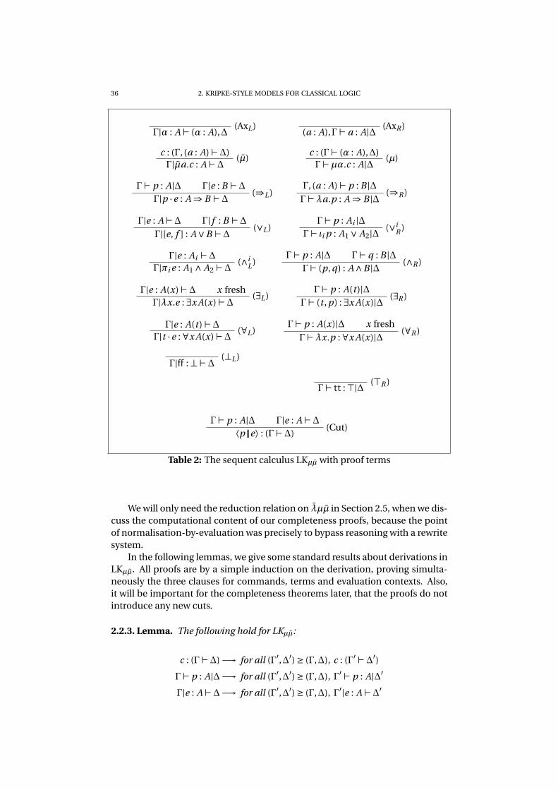
36 2. KRIPKE-STYLE MODELS FOR CLASSICAL LOGIC
(AxL)Γ|α : A ⊢ (α : A),∆
(AxR )(a : A),Γ⊢ a : A|∆
c : (Γ, (a : A) ⊢∆)(µ)
Γ|µa.c : A ⊢∆
c : (Γ⊢ (α : A),∆)(µ)
Γ⊢µα.c : A|∆
Γ⊢ p : A|∆ Γ|e : B ⊢∆(⇒L)
Γ|p ·e : A ⇒ B ⊢∆
Γ, (a : A) ⊢ p : B |∆(⇒R )
Γ⊢λa.p : A ⇒ B |∆
Γ|e : A ⊢∆ Γ| f : B ⊢∆(∨L)
Γ|[e, f ] : A∨B ⊢∆
Γ⊢ p : Ai |∆(∨i
R )Γ⊢ ιi p : A1 ∨ A2|∆
Γ|e : Ai ⊢∆(∧i
L)Γ|πi e : A1 ∧ A2 ⊢∆
Γ⊢ p : A|∆ Γ⊢ q : B |∆(∧R )
Γ⊢ (p, q) : A∧B |∆
Γ|e : A(x) ⊢∆ x fresh(∃L)
Γ|λx.e : ∃x A(x) ⊢∆
Γ⊢ p : A(t )|∆(∃R )
Γ⊢ (t , p) : ∃x A(x)|∆
Γ|e : A(t ) ⊢∆(∀L)
Γ|t ·e : ∀x A(x) ⊢∆
Γ⊢ p : A(x)|∆ x fresh(∀R )
Γ⊢λx.p : ∀x A(x)|∆
(⊥L)Γ|ff : ⊥⊢∆
(⊤R )Γ⊢ tt : ⊤|∆
Γ⊢ p : A|∆ Γ|e : A ⊢∆(Cut)
⟨p‖e⟩ : (Γ⊢∆)
Table 2: The sequent calculus LKµµ with proof terms
We will only need the reduction relation on λµµ in Section 2.5, when we dis-cuss the computational content of our completeness proofs, because the pointof normalisation-by-evaluation was precisely to bypass reasoning with a rewritesystem.
In the following lemmas, we give some standard results about derivations inLKµµ. All proofs are by a simple induction on the derivation, proving simulta-neously the three clauses for commands, terms and evaluation contexts. Also,it will be important for the completeness theorems later, that the proofs do notintroduce any new cuts.
2.2.3. Lemma. The following hold for LKµµ:
c : (Γ⊢∆) −→ for all (Γ′,∆′) ≥ (Γ,∆), c : (Γ′ ⊢∆′)
Γ⊢ p : A|∆−→ for all (Γ′,∆′) ≥ (Γ,∆), Γ′ ⊢ p : A|∆′
Γ|e : A ⊢∆−→ for all (Γ′,∆′) ≥ (Γ,∆), Γ′|e : A ⊢∆′

2.3. KRIPKE-STYLE MODELS, CALL-BY-NAME VARIANT 37
2.2.4. Lemma. The following hold for LKµµ, for any free variable x and any indi-
vidual term t:
c : (Γ⊢∆) −→ c{t/x} : (Γ{t/x} ⊢∆{t/x})
Γ⊢ p : A|∆−→ Γ{t/x} ⊢ p{t/x} : A{t/x}|∆{t/x}
Γ|e : A ⊢∆−→ Γ{t/x}|e{t/x} : A{t/x} ⊢∆{t/x}
2.2.5. Corollary. The following hold for LKµµ, for any x that does not appear in
Γ and ∆, and any individual term t:
Γ⊢ p : A(x)|∆−→ Γ⊢ p{t/x} : A(t )|∆
Γ|e : A(x) ⊢∆−→ Γ|e{t/x} : A(t ) ⊢∆
2.3. Kripke-style models, call-by-name variant
We will now define a notion of model, which is similar to the notion of in-tuitionistic Kripke model, but which we can show sound and complete for theLKµµ sequent calculus. To account for classical logic, we modify the traditionalnotion of Kripke model in the following two ways.
(1) Not taking the forcing relation as primitive. We take as primitive thenotion of “strong refutation”, and define forcing in terms of it. The forc-ing definition we get in this way partially coincides with the traditionaldefinition of forcing, as shown by Proposition 2.3.5.
(2) Allowing certain nodes to validate absurdity. We allow certain possi-ble worlds to be marked as “fallible”, or “exploding”. This approachhas been taken for Kripke models by Veldman [175], for Beth modelsby Friedman [161], and for Boolean models by Krivine (Section 1.1),and seems necessary in order to have a constructive proof of complete-ness, in the view of the meta-mathematical results of Gödel, Kreisel andMcCarthy [120, 136, 135, 137], which preclude constructive proofs ofcompleteness in case one wants to retain that absurdity must never bevalid in a possible world.
2.3.1. Definition. A classical Kripke model, or classical Kripke-style model, isgiven by:
• a preorder (K ,≤) of possible worlds;• a unary relation on worlds (−) ⊥ labelling a world as exploding;• a binary relation (−) : (−) s of strong refutation between worlds and
atomic formulae, such that
for all w ′ ≥ w, w : X s→ w ′ : X s ,
w : ⊥ s is true,
w : ⊤ s iff w ⊥;
• and a domain of quantification D(w) for each world w , such that
for all w ′ ≥ w,D(w) ⊆ D(w ′).
The relation (−) : (−) s of strong refutation is extended from atomic to composite
formulae inductively and by simultaneously defining two new relations, forcingand (non-strong) refutation:
⋆ A formula A is forced in the world w (notation w A) if any world w ′ ≥
w , which strongly refutes A, is exploding;

38 2. KRIPKE-STYLE MODELS FOR CLASSICAL LOGIC
⋆ A formula A is refuted in the world w (notation w : A ) if any worldw ′ ≥ w , which forces A, is exploding;
• w : A∧B s if w : A or w : B ;• w : A∨B s if w : A and w : B ;• w : A ⇒ B s if w A and w : B ;• w : ∀x.A(x) s if w : A(t ) for some t ∈ D(w);• w : ∃x.A(x) s if, for any w ′ ≥ w and t ∈ D(w ′), w : A(t ) .
We have the following basic properties of the defined relations.
2.3.2. Lemma. Strong refutation, forcing and refutation are monotone in any
classical Kripke model.
PROOF. Monotonicity of strong refutation is proved by induction on the com-plexity of the formula, while monotonicity of forcing and of non-strong refuta-tion follows directly from their definitions. �
2.3.3. Lemma. In all worlds w and for all formulae A, if w : A s , then w : A .
PROOF. Immediate, from the definition of refutation. �
We will write w : Γ s , w Γ, and w : Γ , to mean that all formulae of Γare, respectively, strongly forced, refuted, and forced. We now have the follow-ing theorem that says that we can evaluate LKµµ derivations into inhabitants ofclassical Kripke models.
2.3.4. Theorem (Soundness). In any classical Kripke model the following hold:
c : (Γ⊢∆) −→ for any w such that w Γ and w : ∆ , w ⊥
Γ⊢ p : A|∆−→ for any w such that w Γ and w : ∆ , w A
Γ|e : A ⊢∆−→ for any w such that w Γ and w : ∆ , w : A
PROOF. One proves easily the three statements simultaneously, by induc-tion on the derivation. �
It is natural to wonder about the relationship between the intuitionistic andthe classical forcing relations. We characterise that relationship in the next twopropositions.
2.3.5. Proposition. The following hold in any world w of any classical Kripke
model:
w A ⇒ B ←→ for all w ′ ≥ w, w ′ A ⇒ w ′ B(1)
w ∀x.A(x) ←→ for all w ′ ≥ w and t ∈ D(w ′), w ′ A(t )(2)
w ⊥←→ w ⊥(3)
w ⊤←→ true(4)
w A∧B ←→ w A and w B(5)
w A∨B ←− w A or w B(6)
w ∃x.A(x) ←− for some t ∈ D(w), w A(t )(7)
PROOF. (1) Suppose w A ⇒ B , w ′ ≥ w and w ′ A. To show w ′ B welet w ′′ ≥ w ′ and w ′′ : B s and have to show that w ′′ is exploding. Since thenw ′′ : A ⇒ B s holds by monotonicity and Lemma 2.3.3, the claim follows from

2.3. KRIPKE-STYLE MODELS, CALL-BY-NAME VARIANT 39
the definition of w A ⇒ B . For the other direction, suppose a world w ′ ≥ w inwhich A ⇒ B is strongly refuted, i.e. w ′ A and w ′ : B , and we have to showw ′ is exploding. But, this is immediate, since B is also forced by hypothesis (theright-hand side of the equivalence).
(2) By definition, w ∀x.A(x) iff ∀w ′ ≥ w, (∃s ∈ D(w ′).w ′ : A(s) ) ⇒ w ′ ⊥,which is equivalent to the right-hand side of the equivalence thanks to Lemma 2.3.3and refutation being defined in terms of forcing. (We used quantifier symbols atmeta-level.)
(5) Assume w A, w B , w ≤ w ′, and w ′ : A ∧B s . Therefore we havew ′ : A or w ′ : B . Each case leads to w ′ ⊥ since w ′ A, w ′ B with mono-tonicity.
The rest of the cases follow from the definitions and the monotonicity of “ ”and D(−). �
2.3.6. Remark. Note, however, that although the characterisations of our and in-tuitionistic forcing “match” on the fragment {⇒,∧,∀,⊤,⊥}, that does not meanthat a formula in that fragment is forced in our sense if and only if it is forced inthe intuitionistic sense. The law of Peirce ((A ⇒ B) ⇒ A) ⇒ A is one counterex-ample to that, it is classically but not intuitionistically forced; this is so becausein our forcing, hidden under the surface, there lays a notion of refutation whichcan be used.
We now consider the following double-negation translation (·)∗, which is theone of Gödel[87, 161], except that atomic formulae are not doubly negated:
X ∗ := X (X -atomic)
(A∧B)∗ := A∗∧B∗
(A → B)∗ := A∗ → B∗
(∀x.A)∗ := ∀x.A∗
(A∨B)∗ := ¬(¬A∗∧¬B∗)
(∃x.A)∗ := ¬∀x.¬A∗
2.3.7. Proposition. Every classical Kripke model C = (K ,≤,D, s , ⊥) gives rise to
an intuitionistic Kripke model with exploding worlds I = (K ,≤,D, i , ⊥), that
inherits all components of C , except for i which is defined for atomic formulae
by non-strong forcing, i.e.
w i X iff w X
The translation (·)∗ relates C and I , that is, for any world w and any formula A,
we have
w i A∗ iff w A.

40 2. KRIPKE-STYLE MODELS FOR CLASSICAL LOGIC
PROOF. By induction on the complexity of A and by using Lemmas 2.3.5 and2.3.3. We detail only the induction case for ∨, which is the most involved one:
w i (A∨B)∗ ←→
w i ¬(¬A∗∧¬B∗) ←→
(∀w ′ ≥ w) [w ′ i ¬A∗, w ′ i ¬B∗ −→ w ′ i ⊥] ←→
(∀w ′ ≥ w)[ (∀w ′′ ≥ w ′)[w ′′ i A∗ −→ w ′′ i ⊥],
(∀w ′′ ≥ w ′)[w ′′ i B∗ −→ w ′′ i ⊥]
−→ w ′ i ⊥] ←→
(∀w ′ ≥ w)[ (∀w ′′ ≥ w ′)[w ′′ A −→ w ′′ ⊥],
(∀w ′′ ≥ w ′)[w ′′ B −→ w ′′ ⊥]
−→ w ′ ⊥] ←→
(∀w ′ ≥ w) [w ′ : A , w ′ : B −→ w ′ ⊥] ←→
(∀w ′ ≥ w) [w ′ : A∨B s−→ w ′ ⊥] ←→
w A∨B
�
We now define a universal model U analogous to the one for intuitionisticcompleteness from Lemma 2.1.3.
2.3.8. Definition. The Universal classical Kripke model U is obtained by setting:
• K to be the set of contexts (Γ,∆) of LKµµ;• (Γ,∆) ≤ (Γ′,∆′) iff both Γ⊆ Γ
′ and ∆⊆∆′;
• (Γ,∆) : X s iff the sequent Γ|X ⊢∆ is provable without a cut2 in LKµµ;• (Γ,∆) ⊥ iff the sequent Γ⊢∆ is provable without a cut in LKµµ;• for any w , D(w) is the set of individuals of LKµµ(that is, D(−) is a con-
stant function from worlds to sets of individuals).
(−) : (−) s is monotone because of Lemma 2.2.3.
We now have the following theorem.
2.3.9. Theorem (Cut-Free Completeness for U , simplified). For any closed for-
mula A and closed contexts Γ and ∆, the following hold in U :
(Γ,∆) : A −→ {p | Γ⊢ p : A|∆} (↓ −term reify)(1)
(Γ,∆) : A −→ {e | Γ|e : A ⊢∆} (⇓−eval. context reify)(2)
Moreover, the derivations constructed in (1) and (2) are cut-free.
The proof of this version of the theorem was given in our article [109], andit will be given in the form of a λ-term in Section 2.5. We will proceed now toprove a more complex version of it. The reason for doing that is that it is thismore complex version the one that we formalised in Coq, and only for it can weguarantee the computational behaviour described in Section 2.5.
For the more complex version we proceed like in the proof of Lemma 2.1.3.We need two notions of “neutrality”, by analogy to neutral terms of page 32.
2Recall that by “cut” we do not mean the simple application of the CUT rule, but what weexplained on page 35.

2.3. KRIPKE-STYLE MODELS, CALL-BY-NAME VARIANT 41
2.3.10. Definition (NT(−)). A variable declaration a : A is said to be neutral with
respect to provability in the context (Γ,∆) (notation NT(a : A,Γ,∆)), if, for anyevaluation context e and any (Γ′,∆′) ≥ (Γ,∆), we have that
Γ′|e : A ⊢∆
′ −→⟨a‖e⟩ : (Γ′ ⊢∆′).
2.3.11. Definition (NE(−)). A variable declaration α : A is said to be neutral with
respect to refutability in the context (Γ,∆) (notation NE(α : A,Γ,∆)), if, for anyproof term p and any (Γ′,∆′) ≥ (Γ,∆), we have that
Γ′ ⊢ p : A|∆′ −→⟨p‖α⟩ : (Γ′ ⊢∆
′).
We will omit the proof term annotations in order to decrease the level ofdetail, however we remark that the formalisation was carried out with proof termannotations.
2.3.12. Theorem (Cut-Free Completeness for U ). For any closed A,Γ and ∆, the
following hold in U :
(Γ,∆) A −→ Γ⊢ A|∆ (↓ −term reify)(1)
NT(A,Γ,∆) −→ (Γ,∆) A (↑ −term reflect)(2)
(Γ,∆) : A −→ Γ|A ⊢∆ (⇓−eval. context reify)(3)
NE(A,Γ,∆) −→ (Γ,∆) : A (⇑−eval. context reflect)(4)
Moreover, the derivations on the right-hand side of (1) and (3) are cut-free.
PROOF. We proceed by simultaneously proving all four statements by induc-tion on the complexity of A.
Base case. In the base case we have forcing and refutation on atomic formu-lae, which by definition reduce to strong refutation on atomic formulae, whichby definition reduces just to statements about the deductions in LKµµ
(1) Suppose that
(*) ∀(Γ′,∆′) ≥ (Γ,∆). Γ′|X ⊢∆′ → Γ
′ ⊢∆′
Then:(AxL)
Γ|X ⊢ X ,∆(*)
Γ⊢ X ,∆(µ)
Γ⊢ X |∆
(2) The hypothesis is NT(X ,Γ,∆). Given (Γ′,∆′) ≥ (Γ,∆) such that Γ′|X ⊢∆′,
we have:
Γ′|X ⊢∆
′
NT(X ,Γ,∆)Γ′ ⊢∆
′
(3) We have (Γ,∆) : X , i.e.,
(*) ∀(Γ′,∆′) ≥ (Γ,∆).{∀(Γ′′,∆′′) ≥ (Γ′,∆′). Γ′′|X ⊢∆
′′ → Γ′′ ⊢∆
′′}→ Γ
′ ⊢∆′
We can show Γ|X ⊢∆ by applying the (µ)-rule and (*), but we also haveto show the sub-statement in curly brackets of (*):
because X ∈ (X ,Γ) ⊆ Γ′′
(AxR )Γ′′ ⊢ X |∆′′
Γ′′|X ⊢∆
′′
(Cut)Γ′′ ⊢∆
′′
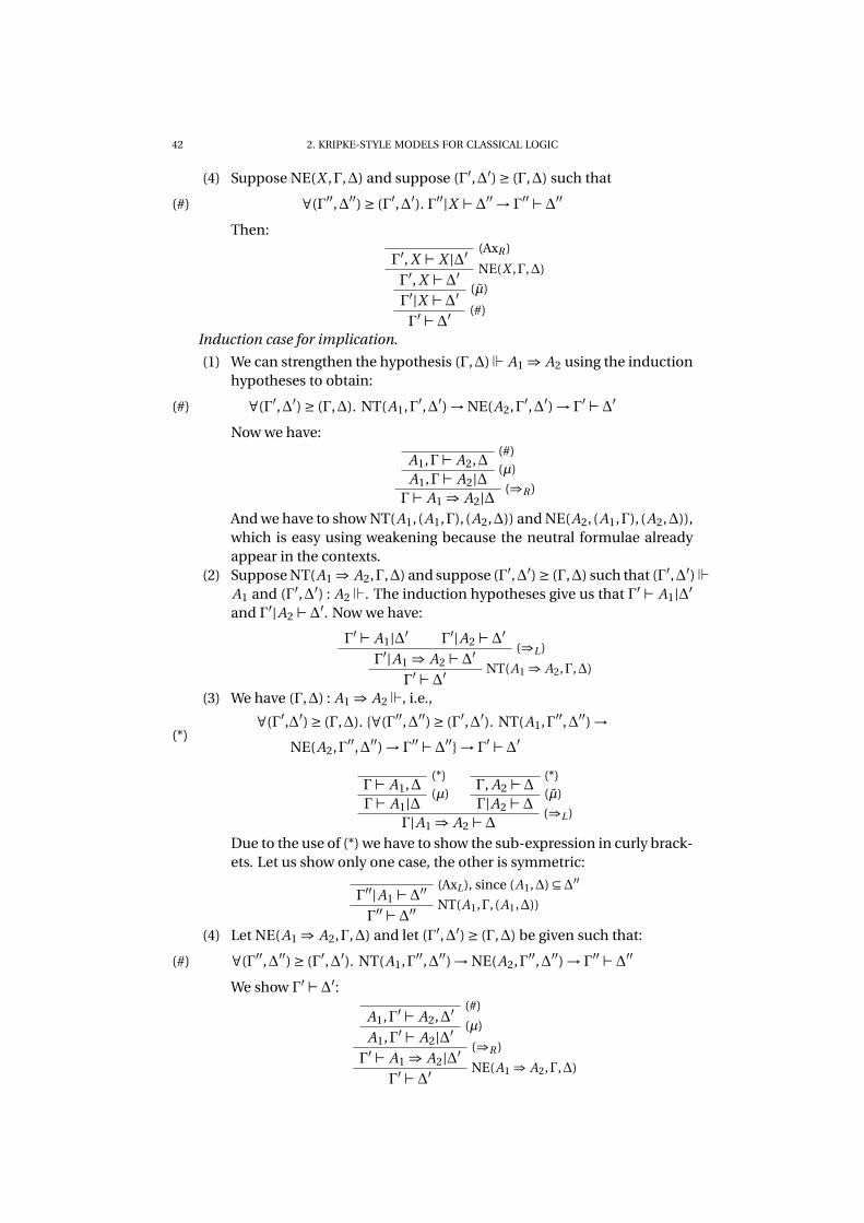
42 2. KRIPKE-STYLE MODELS FOR CLASSICAL LOGIC
(4) Suppose NE(X ,Γ,∆) and suppose (Γ′,∆′) ≥ (Γ,∆) such that
(#) ∀(Γ′′,∆′′) ≥ (Γ′,∆′). Γ′′|X ⊢∆′′ → Γ
′′ ⊢∆′′
Then:(AxR )
Γ′, X ⊢ X |∆′
NE(X ,Γ,∆)Γ′, X ⊢∆
′
(µ)Γ′|X ⊢∆
′
(#)Γ′ ⊢∆
′
Induction case for implication.
(1) We can strengthen the hypothesis (Γ,∆) A1 ⇒ A2 using the inductionhypotheses to obtain:
(#) ∀(Γ′,∆′) ≥ (Γ,∆). NT(A1,Γ′,∆′) → NE(A2,Γ′,∆′) → Γ′ ⊢∆
′
Now we have:(#)
A1,Γ⊢ A2,∆(µ)
A1,Γ⊢ A2|∆ (⇒R )Γ⊢ A1 ⇒ A2|∆
And we have to show NT(A1, (A1,Γ), (A2,∆)) and NE(A2, (A1,Γ), (A2,∆)),which is easy using weakening because the neutral formulae alreadyappear in the contexts.
(2) Suppose NT(A1 ⇒ A2,Γ,∆) and suppose (Γ′,∆′) ≥ (Γ,∆) such that (Γ′,∆′) A1 and (Γ′,∆′) : A2 . The induction hypotheses give us that Γ′ ⊢ A1|∆
′
and Γ′|A2 ⊢∆
′. Now we have:
Γ′ ⊢ A1|∆
′Γ′|A2 ⊢∆
′
(⇒L)Γ′|A1 ⇒ A2 ⊢∆
′
NT(A1 ⇒ A2,Γ,∆)Γ′ ⊢∆
′
(3) We have (Γ,∆) : A1 ⇒ A2 , i.e.,
∀(Γ′,∆′) ≥ (Γ,∆). {∀(Γ′′,∆′′) ≥ (Γ′,∆′). NT(A1,Γ′′,∆′′) →
NE(A2,Γ′′,∆′′) → Γ′′ ⊢∆
′′} → Γ′ ⊢∆
′(*)
(*)Γ⊢ A1,∆
(µ)Γ⊢ A1|∆
(*)Γ, A2 ⊢∆
(µ)Γ|A2 ⊢∆
(⇒L)Γ|A1 ⇒ A2 ⊢∆
Due to the use of (*) we have to show the sub-expression in curly brack-ets. Let us show only one case, the other is symmetric:
(AxL), since (A1,∆) ⊆∆′′
Γ′′|A1 ⊢∆
′′
NT(A1,Γ, (A1,∆))Γ′′ ⊢∆
′′
(4) Let NE(A1 ⇒ A2,Γ,∆) and let (Γ′,∆′) ≥ (Γ,∆) be given such that:
(#) ∀(Γ′′,∆′′) ≥ (Γ′,∆′). NT(A1,Γ′′,∆′′) → NE(A2,Γ′′,∆′′) → Γ′′ ⊢∆
′′
We show Γ′ ⊢∆
′:(#)
A1,Γ′ ⊢ A2,∆′
(µ)A1,Γ′ ⊢ A2|∆
′
(⇒R )Γ′ ⊢ A1 ⇒ A2|∆
′
NE(A1 ⇒ A2,Γ,∆)Γ′ ⊢∆
′
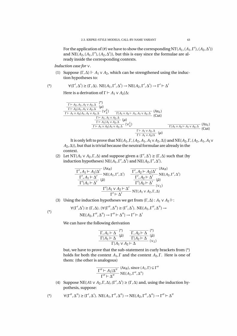
2.3. KRIPKE-STYLE MODELS, CALL-BY-NAME VARIANT 43
For the application of (#) we have to show the corresponding NT(A1, (A1,Γ′), (A2,∆′))and NE(A2, (A1,Γ′), (A2,∆′)), but this is easy since the formulae are al-ready inside the corresponding contexts.
Induction case for ∨.
(1) Suppose (Γ,∆) A1 ∨ A2, which can be strengthened using the induc-tion hypotheses to:
(*) ∀(Γ′,∆′) ≥ (Γ,∆). NE(A1,Γ′,∆′) → NE(A2,Γ′,∆′) → Γ′ ⊢∆
′
Here is a derivation of Γ⊢ A1 ∨ A2|∆:
(*)Γ⊢ A2, A1, A1 ∨ A2,∆
(µ)Γ⊢ A2|A1, A1 ∨ A2,∆
(∨2L)
Γ⊢ A1 ∨ A2|A1, A1 ∨ A2,∆(AxL)
Γ|A1 ∨ A2 ⊢ A1, A1 ∨ A2,∆(Cut)
Γ⊢ A1, A1 ∨ A2,∆(µ)
Γ⊢ A1|A1 ∨ A2,∆(∨1
L)Γ⊢ A1 ∨ A2|A1 ∨ A2,∆
(AxL)Γ|A1 ∨ A2 ⊢ A1 ∨ A2,∆
(Cut)Γ⊢ A1 ∨ A2,∆
(µ)Γ⊢ A1 ∨ A2|∆
It is only left to prove that NE(A1,Γ, (A2, A1, A1∨A2,∆)) and NE(A2,Γ, (A2, A1, A1∨
A2,∆)), but that is trivial because the neutral formulae are already in thecontext.
(2) Let NT(A1 ∨ A2,Γ,∆) and suppose given a (Γ′,∆′) ≥ (Γ,∆) such that (byinduction hypotheses) NE(A1,Γ′,∆′) and NE(A2,Γ′,∆′).
(AxR )Γ′, A1 ⊢ A1|∆
′
NE(A1,Γ′,∆′)Γ′, A1 ⊢∆
′
(µ)Γ′|A1 ⊢∆
′
(AxR )Γ′, A2 ⊢ A2|∆
′
NE(A2,Γ′,∆′)Γ′, A2 ⊢∆
′
(µ)Γ′|A2 ⊢∆
′
(∨L)Γ′|A1 ∨ A2 ⊢∆
′
NT(A1 ∨ A2,Γ,∆)Γ′ ⊢∆
′
(3) Using the induction hypotheses we get from (Γ,∆) : A1 ∨ A2 :
∀(Γ′,∆′) ≥ (Γ,∆). {∀(Γ′′,∆′′) ≥ (Γ′,∆′). NE(A1,Γ′′,∆′′) →
NE(A2,Γ′′,∆′′) → Γ′′ ⊢∆
′′} → Γ′ ⊢∆
′(*)
We can have the following derivation
(*)Γ, A1 ⊢∆
(µ)Γ|A1 ⊢∆
(*)Γ, A2 ⊢∆
(µ)Γ|A2 ⊢∆
(∨L)Γ|A1 ∨ A2 ⊢∆
but, we have to prove that the sub-statement in curly brackets from (*)holds for both the context A1,Γ and the context A2,Γ. Here is one ofthem: (the other is analogous)
(AxR ), since (A1,Γ) ⊆ Γ′′
Γ′′ ⊢ A1|∆
′′
NE(A1,Γ′′,∆′′)Γ′′ ⊢∆
′′
(4) Suppose NE(A1∨ A2,Γ,∆), (Γ′,∆′) ≥ (Γ,∆) and, using the induction hy-pothesis, suppose:
(*) ∀(Γ′′,∆′′) ≥ (Γ′,∆′). NE(A1,Γ′′,∆′′) → NE(A2,Γ′′,∆′′) → Γ′′ ⊢∆
′′

44 2. KRIPKE-STYLE MODELS FOR CLASSICAL LOGIC
(*)Γ′ ⊢ A2, A1,∆′
(µ)Γ′ ⊢ A2|A1,∆′
(∨2L)
Γ′ ⊢ A1 ∨ A2|A1,∆′
NE(A1 ∨ A2,Γ,∆)Γ′ ⊢ A1,∆′
(µ)Γ′ ⊢ A1|∆
′
(∨1L)
Γ′ ⊢ A1 ∨ A2|∆
′
NE(A1 ∨ A2,Γ,∆)Γ′ ⊢∆
′
This constitutes a derivation as required, given that it is easy to proveNE(A1,Γ′, (A2, A1,∆′)) and NE(A2,Γ′, (A2, A1,∆′)) which arise from theuse of (*).
Induction case for ∧.
(1) Let
(*) ∀(Γ′,∆′) ≥ (Γ,∆). NE(A1,Γ′,∆′) or NE(A2,Γ′,∆′) → Γ′ ⊢∆
′
Here is the required derivation:
(*)Γ⊢ A1,∆
(µ)Γ⊢ A1|∆
(*)Γ⊢ A2,∆
(µ)Γ⊢ A2|∆ (∧R )
Γ⊢ A1 ∧ A2|∆
Where it is easy to show that A1 and A2 are neutral in the two casesarising from the use of (*).
(2) Suppose NT(A1 ∧ A2,Γ,∆). To show (Γ,∆) A1 ∧ A2, let (Γ′,∆′) ≥ (Γ,∆)and (NE(A1,Γ′,∆′) or NE(A2,Γ′,∆′)) be true. Without loss of generality,let NE(A1,Γ′,∆′) be true. Then:
(AxR )Γ′, A1 ⊢ A1|∆
′
NE(A1,Γ′,∆′)Γ′, A1 ⊢∆
′
(µ)Γ′|A1 ⊢∆
′
(∧1L)
Γ′|A1 ∧ A2 ⊢∆
′
NT(A1 ∧ A2,Γ′,∆′)Γ′ ⊢∆
′
(3) Suppose (Γ,∆) : A1 ∧ A2 , which can be strengthened using the induc-tion hypotheses to:
∀(Γ′,∆′) ≥ (Γ,∆). {∀(Γ′′,∆′′) ≥ (Γ′,∆′). NE(A1,Γ′′,∆′′) or
NE(A2,Γ′′,∆′′) → Γ′′ ⊢∆
′′} → Γ′ ⊢∆
′(*)
Now we have:(*)
Γ, A1 ∧ A2 ⊢∆(µ)
Γ|A1 ∧ A2 ⊢∆
But we have to show the hypothesis of (*). Let (Γ′′,∆′′) ≥ ((A1∧A2,Γ),∆)and suppose, without loss of generality, that the left disjunct is true, i.e.,we have NE(A1,Γ′′,∆′′). Then:
(AxR )Γ′′ ⊢ A1 ∧ A2|∆
′′
(AxR )Γ′′, A1 ⊢ A1|∆
′′
NE(A1,Γ′′,∆′′)Γ′′, A1 ⊢∆
′′
(µ)Γ′′|A1 ⊢∆
′′
(∧1L)
Γ′′|A1 ∧ A2 ⊢∆
′′
(Cut)Γ′′ ⊢∆
′′

2.3. KRIPKE-STYLE MODELS, CALL-BY-NAME VARIANT 45
(4) Suppose NE(A1 ∧ A2,Γ,∆), (Γ′,∆′) ≥ (Γ,∆) and, using the induction hy-potheses, suppose:
(#) ∀(Γ′′,∆′′) ≥ (Γ′,∆′). NE(A1,Γ′′,∆′′) or NE(A2,Γ′′,∆′′) → Γ′′ ⊢∆
′′
We have:(#)
Γ′ ⊢ A1,∆′
(µ)Γ′ ⊢ A1|∆
′
(#)Γ′ ⊢ A2,∆′
(µ)Γ′ ⊢ A2|∆
′
(∧R )Γ′ ⊢ A1 ∧ A2|∆
′
NE(A1 ∧ A2,Γ,∆)Γ′ ⊢∆
′
where NE(A1,Γ′, (A1,∆′)) and NE(A2,Γ′, (A2,∆′)) arising from the use of(#) are easy to prove, because the formulae are already inside the con-texts.
Induction case for ∀. In the induction cases for ∀ and ∃ we leave out themembership in the domain of individuals D(−) since in U we have a constantdomain and we use the quantifier symbols also at the meta-level, to shorten thenotation.
(1) Let (Γ,∆) ∀x.A(x). Using the induction hypotheses we get:
(*) ∀(Γ′,∆′) ≥ (Γ,∆). (∃t . NE(A(t ),Γ′,∆′)) → Γ′ ⊢∆
′
Here follows the required derivation:
(*)Γ⊢ A(x),∆
(µ)Γ⊢ A(x)|∆
(∀R ), x-freshΓ⊢∀x.A(x)|∆
One easily shows that NE(A(x),Γ, (A(x),∆)).(2) Suppose NT(∀x.A(x),Γ,∆), (Γ′,∆′) ≥ (Γ,∆) and we have t such that, by
induction hypothesis, Γ′|A(t ) ⊢∆′. Here is a derivation of Γ′ ⊢∆
′:
Γ′|A(t ) ⊢∆
′
(∀L)Γ′|∀x.A(x) ⊢∆
′
NT(∀x.A(x),Γ,∆)Γ′ ⊢∆
′
(3) Suppose (Γ,∆) : ∀x.A(x) . We strengthen this using the induction hy-pothesis to:
∀(Γ′,∆′) ≥ (Γ,∆). {∀(Γ′′,∆′′) ≥ (Γ′,∆′).
(∃t . NE(A(t ),Γ′′,∆′′)) → Γ′′ ⊢∆
′′} → Γ′ ⊢∆
′(*)
This(*)
Γ,∀x.A(x) ⊢∆(µ)
Γ|∀x.A(x) ⊢∆
is the derivation we need, in case we prove the sub-expression in curlybrackets of (*). Therefore, suppose (Γ′′,∆′′) ≥ ((∀x.A(x),Γ),∆) and sup-pose a t with NE(A(t ),Γ′′,∆′′). We have to prove Γ
′′ ⊢∆′′:
(AxR )Γ′′ ⊢∀x.A(x)|∆′′
(AxR )Γ′′, A(t ) ⊢ A(t )|∆′′
NE(A(t ),Γ′′,∆′′)Γ′′, A(t ) ⊢∆
′′
(µ)Γ′′|A(t ) ⊢∆
′′
(∀L)Γ′′|∀x.A(x) ⊢∆
′′
(Cut)Γ′′ ⊢∆
′′
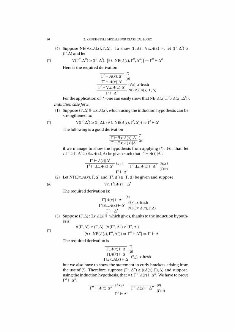
46 2. KRIPKE-STYLE MODELS FOR CLASSICAL LOGIC
(4) Suppose NE(∀x.A(x),Γ,∆). To show (Γ,∆) : ∀x.A(x) , let (Γ′,∆′) ≥
(Γ,∆) and let
(*) ∀(Γ′′,∆′′) ≥ (Γ′,∆′).(∃t . NE(A(t ),Γ′′,∆′′)
)→ Γ
′′ ⊢∆′′
Here is the required derivation:
(*)Γ′ ⊢ A(x),∆′
(µ)Γ′ ⊢ A(x)|∆′
(∀R ), x-freshΓ′ ⊢∀x.A(x)|∆′
NE(∀x.A(x),Γ,∆)Γ′ ⊢∆
′
For the application of (*) one can easily show that NE(A(x),Γ′, (A(x),∆′)).
Induction case for ∃.
(1) Suppose (Γ,∆) ∃x.A(x), which using the induction hypothesis can bestrengthened to:
(*) ∀(Γ′,∆′) ≥ (Γ,∆). (∀t . NE(A(t ),Γ′,∆′)) ⇒ Γ′ ⊢∆
′
The following is a good derivation
(*)Γ⊢∃x.A(x),∆
(µ)Γ⊢∃x.A(x)|∆
if we manage to show the hypothesis from applying (*). For that, lett ,Γ′ ⊇ Γ,∆′ ⊇ (∃x.A(x),∆) be given such that Γ′ ⊢ A(t )|∆′.
Γ′ ⊢ A(t )|∆′
(∃R )Γ′ ⊢∃x.A(x)|∆′
(AxL)Γ′|∃x.A(x) ⊢∆
′
(Cut)Γ′ ⊢∆
′
(2) Let NT(∃x.A(x),Γ,∆) and (Γ′,∆′) ≥ (Γ,∆) be given and suppose
(#) ∀t . Γ′|A(t ) ⊢∆′
The required derivation is:
(#)Γ′|A(x) ⊢∆
′
(∃L), x-freshΓ′|∃x.A(x) ⊢∆
′
NT(∃x.A(x),Γ,∆)Γ′ ⊢∆
′
(3) Suppose (Γ,∆) : ∃x.A(x) which gives, thanks to the induction hypoth-esis:
∀(Γ′,∆′) ≥ (Γ,∆). {∀(Γ′′,∆′′) ≥ (Γ′,∆′).
(∀t . NE(A(t ),Γ′′,∆′′)) ⇒ Γ′′ ⊢∆
′′} ⇒ Γ′ ⊢∆
′(*)
The required derivation is
(*)Γ, A(x) ⊢∆
(µ)Γ|A(x) ⊢∆
(∃L), x-freshΓ|∃x.A(x) ⊢∆
but we also have to show the statement in curly brackets arising fromthe use of (*). Therefore, suppose (Γ′′,∆′′) ≥ ((A(x),Γ),∆) and suppose,using the induction hypothesis, that ∀t . Γ′′|A(t ) ⊢∆
′′. We have to proveΓ′′ ⊢∆
′′:(AxR )
Γ′′ ⊢ A(x)|∆′′
(#)Γ′′|A(x) ⊢∆
′′
(Cut)Γ′′ ⊢∆
′′

2.3. KRIPKE-STYLE MODELS, CALL-BY-NAME VARIANT 47
(4) Suppose NE(∃x.A(x),Γ,∆) and let (Γ′,∆′) ≥ (Γ,∆) such that (Γ′,∆′) ∃x.A(x). Using the induction hypothesis, this last thing strengthens to:
(*) ∀(Γ′′,∆′′) ≥ (Γ′,∆′). (∀t . NE(A(t ),Γ′′,∆′′)) ⇒ Γ′′ ⊢∆
′′
To show Γ′ ⊢ ∆
′, we immediately apply (*) and then have to show thehypothesis: let t ,Γ3,∆3 be such that Γ3 ⊢ A(t )|∆3 and (Γ3,∆3) ≥ (Γ′′,∆′′).Then this is what we are looking for:
Γ3 ⊢ A(t )|∆3 (∃R )Γ3 ⊢∃x.A(x)|∆3 NE(∃x.A(x),Γ,∆)
Γ3 ⊢∆3
Induction case for ⊤.
(1) Immediate, from (⊤R ).(2) Easy, using Proposition 2.3.5.(3) Easy, using Proposition 2.3.5.(4) Easy, a (Cut) with ⊤ and then (⊤R ) and (AxL).
Induction case for ⊥.
(1) Easy, using Proposition 2.3.5.(2) Easy, a (Cut) with ⊥ and then (⊥L) and (AxR ).(3) Immediate, from (⊥L).(4) Immediate, by applying the hypothesis.
All the given derivations are cut-free. By inspection of the proof trees, hav-ing in mind that NT,NE and weakening do not introduce new cuts, we convinceourselves that the completeness theorem indeed produces only cut-free deriva-tions. �
2.3.13. Corollary. For any A,Γ and ∆, the following hold in U :
(1) If A ∈ Γ then (Γ,∆) A.
(2) If B ∈∆ then (Γ,∆) : B .
PROOF. (1) follows from (2) of Theorem 2.3.12, and (2) follows from (4) ofTheorem 2.3.12. �
2.3.14. Corollary (Completeness of Classical Logic). If in every classical Kripke
model, at every possible world, the formula A is forced whenever all the formulae
of Γ are forced and all the formulae of ∆ are refuted, then there exists a derivation
in LKµµ of the sequent Γ⊢ A|∆.
PROOF. If the hypothesis holds for any classical Kripke model, so does ithold for U . To show Γ ⊢ A|∆, by Theorem 2.3.12, it is enough to show that(Γ,∆) B for all B ∈ Γ and (Γ,∆) : C for all C ∈ ∆, something shown in Corol-lary 2.3.13. �
A constructive cut-free completeness theorem can also be used for proofnormalisation.
2.3.15. Corollary (Semantic Cut-Elimination). For all closed contextsΓ,∆, if there
is a derivation of Γ⊢∆, then there is a cut-free derivation of Γ⊢∆.
PROOF. From the hypothesis Γ ⊢ ∆, the soundness theorem applied to U
gives us that there is indeed a cut-free derivation for Γ ⊢ ∆ because the world
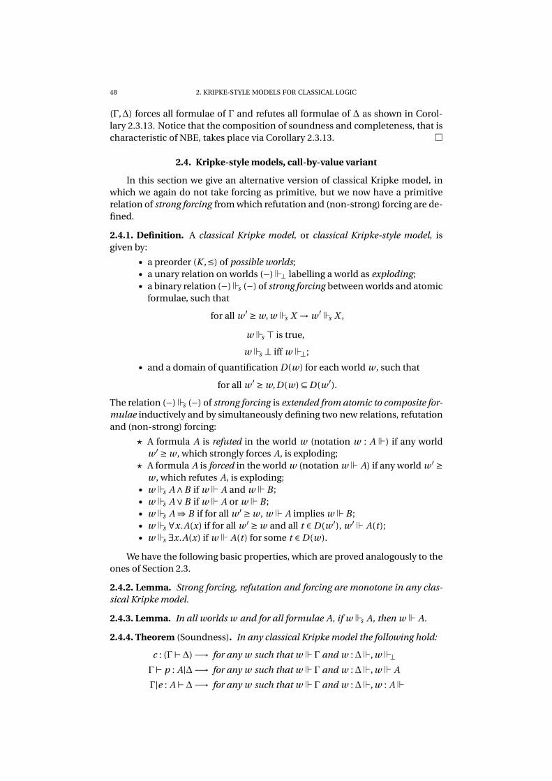
48 2. KRIPKE-STYLE MODELS FOR CLASSICAL LOGIC
(Γ,∆) forces all formulae of Γ and refutes all formulae of ∆ as shown in Corol-lary 2.3.13. Notice that the composition of soundness and completeness, that ischaracteristic of NBE, takes place via Corollary 2.3.13. �
2.4. Kripke-style models, call-by-value variant
In this section we give an alternative version of classical Kripke model, inwhich we again do not take forcing as primitive, but we now have a primitiverelation of strong forcing from which refutation and (non-strong) forcing are de-fined.
2.4.1. Definition. A classical Kripke model, or classical Kripke-style model, isgiven by:
• a preorder (K ,≤) of possible worlds;• a unary relation on worlds (−) ⊥ labelling a world as exploding;• a binary relation (−) s (−) of strong forcing between worlds and atomic
formulae, such that
for all w ′ ≥ w, w s X → w ′ s X ,
w s ⊤ is true,
w s ⊥ iff w ⊥;
• and a domain of quantification D(w) for each world w , such that
for all w ′ ≥ w,D(w) ⊆ D(w ′).
The relation (−) s (−) of strong forcing is extended from atomic to composite for-
mulae inductively and by simultaneously defining two new relations, refutationand (non-strong) forcing:
⋆ A formula A is refuted in the world w (notation w : A ) if any worldw ′ ≥ w , which strongly forces A, is exploding;
⋆ A formula A is forced in the world w (notation w A) if any world w ′ ≥
w , which refutes A, is exploding;• w s A∧B if w A and w B ;• w s A∨B if w A or w B ;• w s A ⇒ B if for all w ′ ≥ w , w A implies w B ;• w s ∀x.A(x) if for all w ′ ≥ w and all t ∈ D(w ′), w ′ A(t );• w s ∃x.A(x) if w A(t ) for some t ∈ D(w).
We have the following basic properties, which are proved analogously to theones of Section 2.3.
2.4.2. Lemma. Strong forcing, refutation and forcing are monotone in any clas-
sical Kripke model.
2.4.3. Lemma. In all worlds w and for all formulae A, if w s A, then w A.
2.4.4. Theorem (Soundness). In any classical Kripke model the following hold:
c : (Γ⊢∆) −→ for any w such that w Γ and w : ∆ , w ⊥
Γ⊢ p : A|∆−→ for any w such that w Γ and w : ∆ , w A
Γ|e : A ⊢∆−→ for any w such that w Γ and w : ∆ , w : A
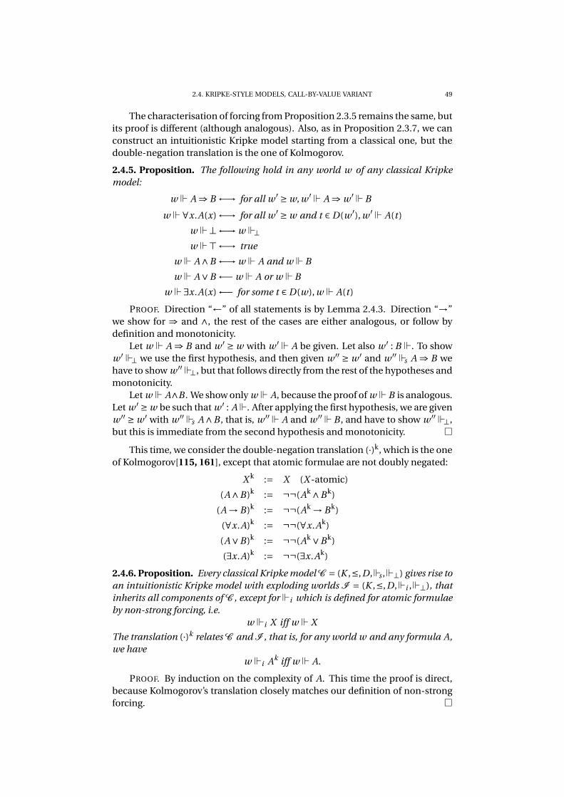
2.4. KRIPKE-STYLE MODELS, CALL-BY-VALUE VARIANT 49
The characterisation of forcing from Proposition 2.3.5 remains the same, butits proof is different (although analogous). Also, as in Proposition 2.3.7, we canconstruct an intuitionistic Kripke model starting from a classical one, but thedouble-negation translation is the one of Kolmogorov.
2.4.5. Proposition. The following hold in any world w of any classical Kripke
model:
w A ⇒ B ←→ for all w ′ ≥ w, w ′ A ⇒ w ′ B
w ∀x.A(x) ←→ for all w ′ ≥ w and t ∈ D(w ′), w ′ A(t )
w ⊥←→ w ⊥
w ⊤←→ true
w A∧B ←→ w A and w B
w A∨B ←− w A or w B
w ∃x.A(x) ←− for some t ∈ D(w), w A(t )
PROOF. Direction “←” of all statements is by Lemma 2.4.3. Direction “→”we show for ⇒ and ∧, the rest of the cases are either analogous, or follow bydefinition and monotonicity.
Let w A ⇒ B and w ′ ≥ w with w ′ A be given. Let also w ′ : B . To showw ′ ⊥ we use the first hypothesis, and then given w ′′ ≥ w ′ and w ′′ s A ⇒ B wehave to show w ′′ ⊥, but that follows directly from the rest of the hypotheses andmonotonicity.
Let w A∧B . We show only w A, because the proof of w B is analogous.Let w ′ ≥ w be such that w ′ : A . After applying the first hypothesis, we are givenw ′′ ≥ w ′ with w ′′ s A∧B , that is, w ′′ A and w ′′ B , and have to show w ′′ ⊥,but this is immediate from the second hypothesis and monotonicity. �
This time, we consider the double-negation translation (·)k, which is the oneof Kolmogorov[115, 161], except that atomic formulae are not doubly negated:
X k := X (X -atomic)
(A∧B)k := ¬¬(Ak ∧B k)
(A → B)k := ¬¬(Ak → B k)
(∀x.A)k := ¬¬(∀x.Ak)
(A∨B)k := ¬¬(Ak ∨B k)
(∃x.A)k := ¬¬(∃x.Ak)
2.4.6. Proposition. Every classical Kripke model C = (K ,≤,D, s , ⊥) gives rise to
an intuitionistic Kripke model with exploding worlds I = (K ,≤,D, i , ⊥), that
inherits all components of C , except for i which is defined for atomic formulae
by non-strong forcing, i.e.
w i X iff w X
The translation (·)k relates C and I , that is, for any world w and any formula A,
we have
w i Ak iff w A.
PROOF. By induction on the complexity of A. This time the proof is direct,because Kolmogorov’s translation closely matches our definition of non-strongforcing. �

50 2. KRIPKE-STYLE MODELS FOR CLASSICAL LOGIC
2.4.7. Definition. The Universal classical Kripke model U is obtained by setting:
• K to be the set of contexts (Γ,∆) of LKµµ;• (Γ,∆) ≤ (Γ′,∆′) iff both Γ⊆ Γ
′ and ∆⊆∆′;
• (Γ,∆) s X iff the sequent Γ⊢ X |∆ is provable without a cut in LKµµ;• (Γ,∆) ⊥ iff the sequent Γ⊢∆ is provable without a cut in LKµµ;• for any w , D(w) is the set of individuals of LKµµ(that is, D(−) is a con-
stant function from worlds to sets of individuals).
(−) s (−) is monotone because of Lemma 2.2.3.
This time we will not prove a more complex version of the theorem, becauseit is the simpler version that we formalised in Coq.
2.4.8. Theorem (Cut-Free Completeness for U ). For any closed formula A and
closed contexts Γ and ∆, the following hold in U :
(Γ,∆) A −→ {p | Γ⊢ p : A|∆} (↓ −term reify)(1)
(Γ,∆) : A −→ {e | Γ|e : A ⊢∆} (⇓−eval. context reify)(2)
Moreover, the derivations constructed in (1) and (2) are cut-free.
PROOF. We will once again skip writing the proof term annotations in orderto decrease the level of detail. The algorithm behind this proof that concentrateson proof terms is given in Table 7, page 55.
Base case. Let (Γ,∆) A for A-atomic. By definition, this is
(*) ∀(Γ′,∆′
)≥ (Γ,∆) .
(∀
(Γ′′,∆′′
)≥
(Γ′,∆′
). Γ′′ ⊢ A|∆′′ → Γ
′′ ⊢∆′′)→ Γ
′ ⊢∆′.
We can deriveΓ⊢ A|∆by first applying the (µ)rule, and then (*) with the (AxL)rule.Let (Γ,∆) : A for A-atomic, that is, let
(#) ∀(Γ′,∆′
)≥ (Γ,∆) . Γ′|A ⊢∆
′ → Γ′ ⊢∆
′.
The derivation of Γ|A ⊢∆ is immediate by applying (µ), (*) and (AxR ).Induction case for (∧). Let (Γ,∆) A∧B , that is,
(*) ∀(Γ′,∆′
)≥ (Γ,∆) .
(∀
(Γ′′,∆′′
)≥
(Γ′,∆′
).
(Γ′′,∆′′
) A and
(Γ′′,∆′′
) B → Γ
′′ ⊢∆′′)→ Γ
′ ⊢∆′.
We derive Γ⊢ A∧B |∆ by the rule (∧R )and show each of the conjuncts separately.For example, to show Γ⊢ A|∆, we apply (µ), then (*), and then, given
(Γ, (A,∆)) A and (Γ, (A,∆)) B ,
we have to show Γ⊢ A,∆, but that is immediate by the induction hypothesis (1)and the (AxL)rule.
Let (Γ,∆) : A∧B , that is,
(#) ∀(Γ′,∆′
)≥ (Γ,∆) .
(Γ′,∆′
) A and
(Γ′,∆′
) B → Γ
′ ⊢∆′.
To derive Γ|A ∧ B ⊢ ∆, we apply (µ)and then (#). We have to prove each of((A∧B ,Γ),∆) A and ((A∧B ,Γ),∆) B separately. Let (Γ′,∆′) ≥ ((A ∧B ,Γ),∆)and let (Γ′,∆′) : A . We show Γ
′ ⊢ ∆′ by using (AxR ), (∧1
L) and the inductionhypothesis (2). The proof of ((A∧B ,Γ),∆) B is analogous.

2.4. KRIPKE-STYLE MODELS, CALL-BY-VALUE VARIANT 51
Induction case for (∨). Let (Γ,∆) A∨B , that is,
(*) ∀(Γ′,∆′
)≥ (Γ,∆) .
(∀
(Γ′′,∆′′
)≥
(Γ′,∆′
).
(Γ′′,∆′′
) A or
(Γ′′,∆′′
) B → Γ
′′ ⊢∆′′)→ Γ
′ ⊢∆′.
We derive Γ|A∨B ⊢∆ by the rule (µ)and applying (*). Then, given
((A∨B ,Γ) ,∆) A or ((A∨B ,Γ) ,∆) B ,
we have to show that A∨B ,Γ⊢∆. This is done by case distinction; if ((A∨B ,Γ) ,∆) A, then we use the induction hypothesis (1) to obtain A∨B ,Γ⊢ A|∆, and hence,using (∨1
R ) and (AxL)we get A∨B ,Γ⊢∆. The case ((A∨B ,Γ) ,∆) A is analogous.Let (Γ,∆) : A∨B , that is,
(#) ∀(Γ′,∆′
)≥ (Γ,∆) .
(Γ′,∆′
) A or
(Γ′,∆′
) B → Γ
′ ⊢∆′.
To derive Γ|A ∨B ⊢∆, we apply (∨L) and we have to derive each of Γ|A ⊢∆ andΓ|B ⊢∆ separately. We only derive the first one, by applying (µ), then (Cut)with(AxR )and applying induction hypothesis (2) for A: given ((A,Γ),∆) s A, we canuse (#) and Lemma 2.4.3 to derive (A,Γ) ⊢∆.
Induction case for (⇒). Let (Γ,∆) : A ⇒ B , that is,
(*) ∀(Γ′,∆′
)≥ (Γ,∆) .
(∀
(Γ′′,∆′′
)≥
(Γ′,∆′
).
[∀(Γ′′′,∆′′′) ≥ (Γ′′,∆′′). (Γ′′′,∆′′′) A → (Γ′′′,∆′′′) B
]→ Γ
′′ ⊢∆′′)→ Γ
′ ⊢∆′
To derive Γ⊢ A ⇒ B |∆, we apply (⇒R ), then (µ), then (*), and, given
(#) ∀(Γ3,∆3) ≥ ((A,Γ), (B ,∆)). (Γ3,∆3) A → (Γ3,∆3) B ,
we have to derive Γ3 ⊢ ∆3. We apply (Cut)with the formula B , and then use IH(1) followed by (#). Now, we have to show (Γ3,∆3) A. Let (Γ4,∆4) ≥ (Γ3,∆3) and(Γ4,∆4) : A . We derive Γ4 ⊢ ∆4 by a (Cut)with (AxR )and IH (2) applied to thelast hypothesis.
Let now (Γ,∆) : A ⇒ B , that is,(#)∀
(Γ′,∆′
)≥ (Γ,∆) .
[∀(Γ′′,∆′′) ≥ (Γ′,∆′). (Γ′′,∆′′) A → (Γ′′,∆′′) B
]→ Γ
′ ⊢∆′.
We deriveΓ|A ⇒ B ⊢∆by applying (µ), then (#), and then, given ((A ⇒ B ,Γ),∆) A and ((A ⇒ B ,Γ),∆) : B , we can derive A ⇒ B ,Γ ⊢ ∆ by a (Cut)with A ⇒ B ,using the evaluation context constructed by combining the last two hypothesiswith IH (1) and IH (2), respectively.
The induction cases for ∀ and ∃ are proved analogously to those of ⇒ and ∨,but more simply. The cases of ⊤ and ⊥ are trivial. �
2.4.9. Corollary. For any sentence A and contexts of sentences Γ,∆, the following
hold for U :
(1) If A ∈ Γ then (Γ,∆) A.
(2) If B ∈∆ then (Γ,∆) : B .
PROOF. (1) Assume A ∈ Γ, (Γ′,∆′) ≥ (Γ,∆) and (Γ′,∆′) : A . Then, byTheorem 2.4.8, Γ′ | A ⊢∆
′, hence we can obtain a cut-free proof of Γ′ ⊢
∆′ using left contraction (page 34).
(2) Assume B ∈ ∆, (Γ′,∆′) ≥ (Γ,∆) and (Γ′,∆′) s B . Then, by Lemma 2.4.3and Theorem 2.4.8, Γ′ ⊢ B |∆′, hence we can obtain a cut-free proof ofΓ′ ⊢∆
′ using right contraction (page 35).
52 2. KRIPKE-STYLE MODELS FOR CLASSICAL LOGIC
�
2.4.10. Corollary (Completeness of Classical Logic). If in every classical Kripke
model, at every possible world, the formula A is forced whenever all the formulae
of Γ are forced and all the formulae of ∆ are refuted, then there exists a derivation
in LKµµ of the sequent Γ⊢ A|∆.
PROOF. Analogous to Corollary 2.3.14, by using Corollary 2.4.9. �
We again have the following corollary.
2.4.11. Corollary (Semantic Cut-Elimination). For all contexts Γ,∆ of sentences,
if there is a derivation of Γ⊢∆, then there is a cut-free derivation of Γ⊢∆.
PROOF. From the hypothesis Γ ⊢ ∆, the soundness theorem applied to U
gives us that there is indeed a cut-free derivation for Γ ⊢ ∆ because the world(Γ,∆) forces all formulae of Γ and refutes all formulae of ∆ as shown in Corol-lary 2.4.9. Note, however, that the proof of Corollary 2.4.9 is not analogous to theone of Corollary 2.3.13. �
2.5. Computational content
So far, we have not justified the headings “call-by-name variant” and “call-by-value variant” of Sections 2.3 and 2.4. We do that in this section by show-ing that the computational content of Corollary 2.3.15 is λµµ-command nor-malisation in call-by-name strategy, while the computational content of Corol-lary 2.4.11 is call-by-value normalisation.
One of the strengths of the λµµ-calculus is that it is able to very simply char-acterise call-by-name (CBN) and call-by-value (CBV) evaluation strategies. If weconsider again the reduction rules of Definition 2.2.2, we see that there is a crit-ical pair ⟨µα.c‖µa.c ′⟩ for which we do not know whether to first apply the →µ
rule or the →µ rule. As it is shown in [53], giving priority to the →µ rule gives riseto a CBN reduction strategy, while giving priority to the →µ rule gives rise to aCBV strategy.
Now, since we have formalised our proofs in the Coq proof assistant, whichis based on a constructive theory of types, we can compute with the proofs di-rectly, and see how “semantic cut-elimination” is performed. This is the tech-nique of proof by reflection that we mentioned in Section 1.5. We restrict our-selves to the propositional fragment, because we did not formalise the quantifierversion of the CBN classical Kripke model (see Section 2.6). The results are givenin Tables 3 and 4.
We can see that Corollary 2.3.15 reduces all commands in perfect accordwith the reduction relation of Definition 2.2.2 for CBN strategy, however, Corol-lary 2.4.11 is not in perfect accord, because, although it reduces all commandsaccording to the CBV strategy, there are two η-redexes dangling on the evalua-tion context side. Hence, one is forced to perform two more steps of reduction,
⟨p‖µd .
⟨µδ.⟨d‖δ⟩‖β
⟩⟩→µ
⟨µδ.
⟨p‖δ
⟩‖β
⟩→µ
⟨p‖β
⟩,
in order to obtain a final cut-free form.We have tracked this difference of behaviour down to the difference in the
proofs of Corollaries 2.3.13 and 2.4.9. However, we do not claim that the sameproblem with a final η-redex would happen if the simplified Theorem 2.3.9 had

2.6. ASPECTS OF THE COQ FORMALISATION 53
⟨µα.
⟨a‖β
⟩‖µb.
⟨c‖γ
⟩⟩→
⟨c‖γ
⟩⟨µα.⟨a‖α⟩‖β
⟩→
⟨a‖β
⟩⟨λa.a‖b ·β
⟩→
⟨b‖β
⟩
⟨(a,b)‖π1α⟩→ ⟨a‖α⟩
⟨(a,b)‖π2α⟩→ ⟨b‖α⟩⟨ι1a‖[α,β]
⟩→⟨a‖α⟩
⟨ι2a‖[α,β]
⟩→
⟨a‖β
⟩
(different letters stand for distinct entities)
Table 3: Algorithmic behaviour of the CBN models
⟨µα.
⟨a‖β
⟩‖µb.
⟨c‖γ
⟩⟩→
⟨a‖µd .
⟨µδ.⟨d‖δ⟩‖β
⟩⟩→2 ⟨
a‖β⟩
⟨µα.⟨a‖α⟩‖β
⟩→
⟨a‖µd .
⟨µδ.⟨d‖δ⟩‖β
⟩⟩→2 ⟨
a‖β⟩
⟨λa.a‖b ·β
⟩→
⟨b‖µd .
⟨µδ.⟨d‖δ⟩‖β
⟩⟩→2 ⟨
b‖β⟩
⟨(a,b)‖π1α⟩→⟨
a‖µd .⟨µδ.⟨d‖δ⟩‖α
⟩⟩→2 ⟨a‖α⟩
⟨(a,b)‖π2α⟩→⟨
b‖µd .⟨µδ.⟨d‖δ⟩‖α
⟩⟩→2 ⟨b‖α⟩
⟨ι1a‖[α,β]
⟩→
⟨a‖µd .
⟨µδ.⟨d‖δ⟩‖α
⟩⟩→2 ⟨a‖α⟩
⟨ι2a‖[α,β]
⟩→
⟨a‖µd .
⟨µδ.⟨d‖δ⟩‖β
⟩⟩→2 ⟨
a‖β⟩
(different letters stand for distinct entities)
Table 4: Algorithmic behaviour of the CBV models
been used for computation. It may well be that a different notion of call-by-value model is necessary in order to obtain full normalisation, for example amodel along the lines of the CPS translation of Section 4.2.
We have manually extracted the algorithms behind the proofs of Theorems2.3.9, 2.3.12 and 2.4.8, because the machine extracted algorithms of 2.3.12 and2.4.8 contain too many details to be comprehensible, while 2.3.9 was not at allformalised. They are given in Tables 5, 6, and 7. For meta-level abstraction andapplication we use “7→” and “·”, for meta-level pair projections we use “fst” and“snd”, while for meta-level left- and right-injection we use “inl” and “inr”. Defi-nition by cases is written as usually in Mathematics, pairs are written by (H ,G),and there is a shortcut “ret ·H” which stands for “G 7→G ·H”.
2.6. Aspects of the Coq formalisation
The source code of the Coq formalisation is available at the address ❤tt♣✿✴✴✇✇✇✳❧✐①✳♣♦❧②t❡❝❤♥✐q✉❡✳❢r✴⑦❞❛♥❦♦✴❝♦❞❡. We had formalised first the proofof Theorem 2.3.12, only for the fragment {⇒,∧,∨}, and then we rewrote theformalisation for Theorem 2.4.8, in parallel to developing the formalisation ofChapter 3. These last two formalisations include also the quantifiers. We re-mark that the proof of Theorem 2.4.8 is analogous to the one of Theorem 2.3.9,

54 2. KRIPKE-STYLE MODELS FOR CLASSICAL LOGIC
↓A : (Γ,∆) A → {p | Γ⊢ p : A|∆}
↑A : NT(a : A,Γ,∆) → (Γ,∆) A
⇓A : (Γ,∆) : A → {e | Γ|e : A ⊢∆}
⇑A : NE(α : A,Γ,∆) → (Γ,∆) : A
↓X := H 7→µα.H ·α
↑X := H 7→ H ′ 7→ H ·H ′
⇓X := H 7→ µa.H · (e 7→ ⟨a‖e⟩)
⇑X := H 7→ H ′ 7→ H ·(µα.H ′ ·α
)
↓A∧B := H 7→
(µα.H ·
(inl ·
(⇑A p 7→ ⟨p‖α⟩
)),
µα.H ·(inr ·
(⇑B p 7→ ⟨p‖α⟩
)))
↑A∧B := H 7→ H ′ 7→
{H ·
(ι1
(µa.H ′′ ·
(↑A e 7→ ⟨a‖e⟩
)))if H ′ = inl ·H ′′
H ·(ι2
(µa.H ′′ ·
(↑B e 7→ ⟨a‖e⟩
)))if H ′ = inr ·H ′′
⇓A∧B := H 7→ µa.H ·
(H ′ 7→
{⟨a‖π1
(µb.H ′′ ·
(↑A e 7→ ⟨b‖e⟩
))⟩, if H ′ = inl ·H ′′
⟨a‖π2(µb.H ′′ ·
(↑B e 7→ ⟨b‖e⟩
))⟩, if H ′ = inr ·H ′′
)
⇑A∧B := H 7→ H ′ 7→ H ·
(µα.H ′ ·
(inl ·
(⇑A p 7→ ⟨p‖α⟩
)),
µα.H ′ ·(inr ·
(⇑B p 7→ ⟨p‖α⟩
)))
↓A∨B := H 7→µγ.⟨ι1
(µα.
⟨ι2
(µβ.H ·
(⇑A p 7→ ⟨p‖α⟩,⇑B p 7→ ⟨p‖β⟩
))‖γ
⟩)‖γ
⟩
↑A∨B := H 7→ H ′ 7→ H ·
[µa.
(fst ·H ′
)·(↑A e 7→ ⟨a‖e⟩
),
µa.(snd ·H ′
)·(↑B e 7→ ⟨a‖e⟩
)]
⇓A∨B := H 7→
[µa.H ·
(H ′ 7→
(fst ·H ′
)·(↑A e 7→ ⟨a‖e⟩
)),
µa.H ·(H ′ 7→
(snd ·H ′
)·(↑B e 7→ ⟨a‖e⟩
))]
⇑A∨B := H 7→ H ′ 7→ H ·(ι1
(µα.H ·
(ι2
(µβ.H ′ ·
(⇑A p 7→ ⟨p‖α⟩,⇑B p 7→ ⟨p‖β⟩
)))))
↓A⇒B := H 7→λa.µα.H ·(↑A e 7→ ⟨a‖e⟩
)·(⇑B p 7→ ⟨p‖α⟩
)
↑A⇒B := H 7→ H ′ 7→ H ·((↓A fst ·H ′
)·(⇓B snd ·H ′
))
⇓A⇒B := H 7→(µα.H ·
(↑A p 7→ ⟨p‖α⟩
))·(µa.H ·
(⇑B e 7→ ⟨a‖e⟩
))
⇑A⇒B := H 7→ H ′ 7→ H ·(λa.µα.H ′ ·
(↓A e 7→ ⟨a‖e⟩
)·(⇓B p 7→ ⟨p‖α⟩
))
Table 5: The normalisation algorithm behind Theorem 2.3.12
which we gave in our article [109], therefore obtaining a formal version of thetheorem from the article should not be too difficult.
The way of representing binders, substitutions and the co-finite quantifica-tion rule is the same as in Section 1.5, except that the definition of formulae doesnot include Henkin constants. However, the definition of individual terms fromthe formalisations of Chapters 2 and 3, allows to have multiple arguments forpredicate and function symbols, which means that these completeness proofsare more prepared for practical application inside Coq, that the one of Chap-ter 1. Formally, in type theory, fixed points for working with such individual
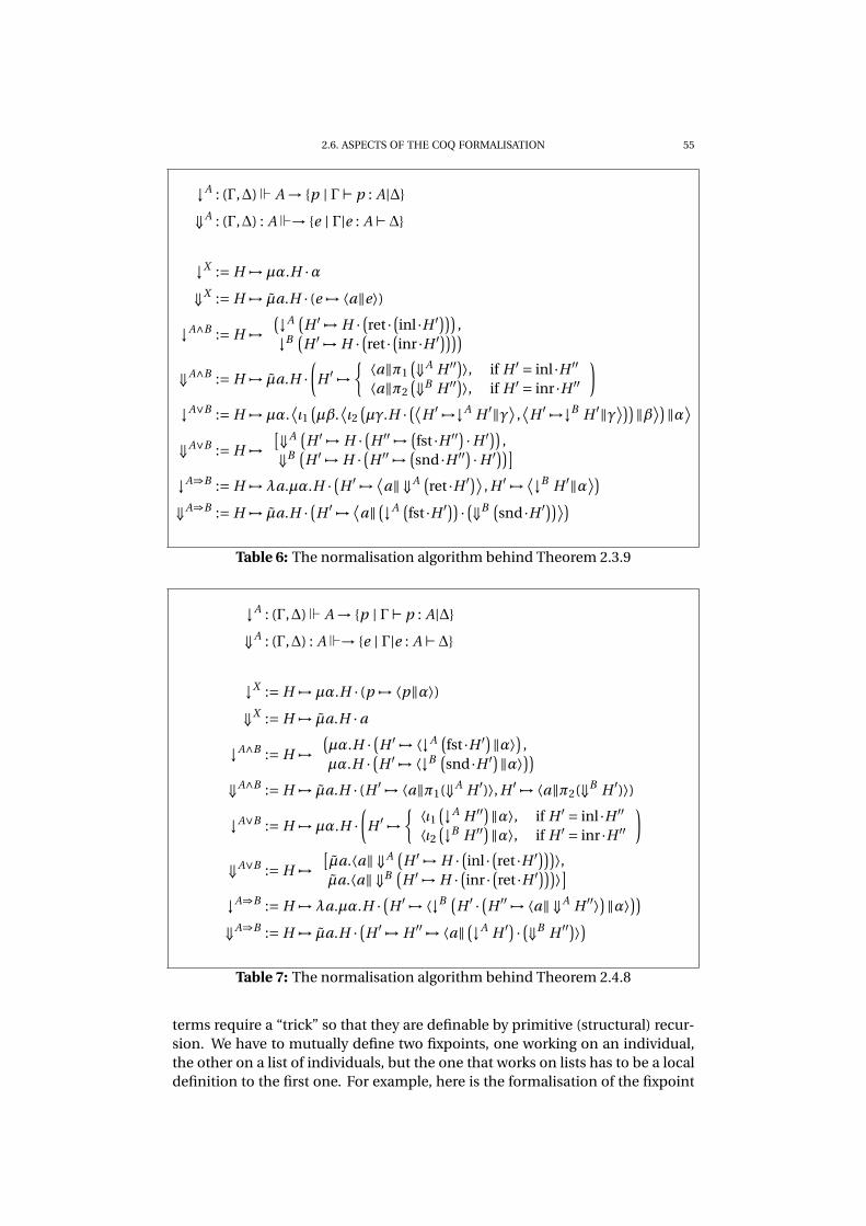
2.6. ASPECTS OF THE COQ FORMALISATION 55
↓A : (Γ,∆) A → {p | Γ⊢ p : A|∆}
⇓A : (Γ,∆) : A → {e | Γ|e : A ⊢∆}
↓X := H 7→µα.H ·α
⇓X := H 7→ µa.H · (e 7→ ⟨a‖e⟩)
↓A∧B := H 7→
(↓A
(H ′ 7→ H ·
(ret ·
(inl ·H ′
))),
↓B(H ′ 7→ H ·
(ret ·
(inr ·H ′
))))
⇓A∧B := H 7→ µa.H ·
(H ′ 7→
{⟨a‖π1
(⇓A H ′′
)⟩, if H ′ = inl ·H ′′
⟨a‖π2(⇓B H ′′
)⟩, if H ′ = inr ·H ′′
)
↓A∨B := H 7→µα.⟨ι1
(µβ.
⟨ι2
(µγ.H ·
(⟨H ′ 7→↓A H ′‖γ
⟩,⟨
H ′ 7→↓B H ′‖γ⟩))
‖β⟩)‖α
⟩
⇓A∨B := H 7→
[⇓A
(H ′ 7→ H ·
(H ′′ 7→
(fst ·H ′′
)·H ′
)),
⇓B(H ′ 7→ H ·
(H ′′ 7→
(snd ·H ′′
)·H ′
))]
↓A⇒B := H 7→λa.µα.H ·(H ′ 7→
⟨a‖ ⇓A
(ret ·H ′
)⟩, H ′ 7→
⟨↓B H ′‖α
⟩)
⇓A⇒B := H 7→ µa.H ·(H ′ 7→
⟨a‖
(↓A
(fst ·H ′
))·(⇓B
(snd ·H ′
))⟩)
Table 6: The normalisation algorithm behind Theorem 2.3.9
↓A : (Γ,∆) A → {p | Γ⊢ p : A|∆}
⇓A : (Γ,∆) : A → {e | Γ|e : A ⊢∆}
↓X := H 7→µα.H · (p 7→ ⟨p‖α⟩)
⇓X := H 7→ µa.H ·a
↓A∧B := H 7→
(µα.H ·
(H ′ 7→ ⟨↓A
(fst ·H ′
)‖α⟩
),
µα.H ·(H ′ 7→ ⟨↓B
(snd ·H ′
)‖α⟩
))
⇓A∧B := H 7→ µa.H · (H ′ 7→ ⟨a‖π1(⇓A H ′)⟩, H ′ 7→ ⟨a‖π2(⇓B H ′)⟩)
↓A∨B := H 7→µα.H ·
(H ′ 7→
{⟨ι1
(↓A H ′′
)‖α⟩, if H ′ = inl ·H ′′
⟨ι2(↓B H ′′
)‖α⟩, if H ′ = inr ·H ′′
)
⇓A∨B := H 7→
[µa.⟨a‖ ⇓A
(H ′ 7→ H ·
(inl ·
(ret ·H ′
)))⟩,
µa.⟨a‖ ⇓B(H ′ 7→ H ·
(inr ·
(ret ·H ′
)))⟩]
↓A⇒B := H 7→λa.µα.H ·(H ′ 7→ ⟨↓B
(H ′ ·
(H ′′ 7→ ⟨a‖ ⇓A H ′′⟩
)‖α⟩
))
⇓A⇒B := H 7→ µa.H ·(H ′ 7→ H ′′ 7→ ⟨a‖
(↓A H ′
)·(⇓B H ′′
)⟩)
Table 7: The normalisation algorithm behind Theorem 2.4.8
terms require a “trick” so that they are definable by primitive (structural) recur-sion. We have to mutually define two fixpoints, one working on an individual,the other on a list of individuals, but the one that works on lists has to be a localdefinition to the first one. For example, here is the formalisation of the fixpoint

56 2. KRIPKE-STYLE MODELS FOR CLASSICAL LOGIC
which substitutes the free variable k of the individual term a with the individualterm d :
❋✐①♣♦✐♥t subst indiv (k:nat)(a:indiv)(d:indiv) {str✉❝t a} : indiv :=❧❡t subst list := fix subst list (l:list indiv) {str✉❝t l} : list indiv :=♠❛t❝❤ l ✇✐t❤
| nil ⇒ nil
| cons a’ l’ ⇒ cons (subst indiv k a’ d) (subst list l’)❡♥❞ ✐♥
♠❛t❝❤ a ✇✐t❤
| func f ld ⇒
func f (subst list ld)| fvar x ⇒ fvar x
| bvar i ⇒ ✐❢ beq nat k i t❤❡♥ d ❡❧s❡ bvar i
❡♥❞.
This kind of definition is analogous to the one of the Ackermann functionusing higher-type primitive recursion.
Coq was clever in being able to generate for us, using the ❙❝❤❡♠❡ command,a mutual induction predicate for derivations of LKµµ. A slight anomaly was,however, that it knew how to generate such predicates only for sort Prop, notsort Type.
We can also say that in general the separation Prop/Set of Coq was not veryconvenient. While “usually”, when an algorithm and its correctness proof arewell separated, this distinction makes extracted terms be more readable, in thesekind of meta-theoretic algorithms, logic is an integral part of the computation. Itwas thus necessary to rewrite a couple of lemmas from the Coq standard library,that deal with lists and number comparison, so that they live in Set instead ofProp.
2.7. Related and future work
2.7.1. Normalisation by evaluation. In Section 2.5 we showed that the com-putational content of the completeness proofs of this chapter is cut-elimination,or proof normalisation. However, we did not obtain a result as good as the oneof Berger and Schwichtenberg [33], because they showed that the input and theoutput of their NBE algorithm are βη-equal. In future, we would like to extendour work in that direction. We will have to be more careful when treating η-equality in the context of λµµ because a more finely grained reduction rule for(→⇒) will then be needed (see the Habilitation thesis of Herbelin [98]).
The work of Okada [147] is related to NBE for classical logic. Directly in-spired by Girard’s phase semantics [80] for linear logic, Okada shows that thereis a uniform cut-eliminating completeness proof for various extensions of in-tuitionistic linear logic, including classical predicate calculus. His approach ismore algebraic than ours. While he defines his phase semantics from an ab-stract monoid structure and uses set comprehension to interpret the logical con-stants, we rely on a Kripke-style model, which is nothing else but a continuationsmonad. We are not aware of any explicit algorithms for cut-elimination that fol-low his approach.
Okada’s semantics is related to Sambin’s pre-topology semantics [153].
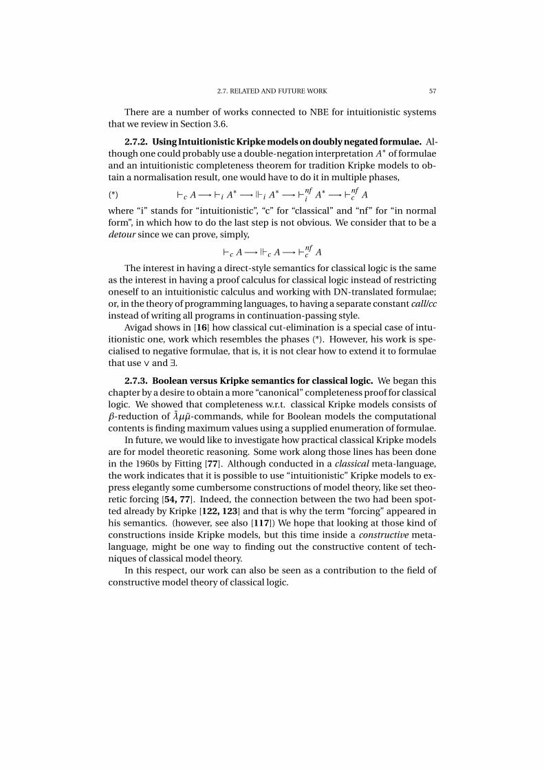
2.7. RELATED AND FUTURE WORK 57
There are a number of works connected to NBE for intuitionistic systemsthat we review in Section 3.6.
2.7.2. Using Intuitionistic Kripke models on doubly negated formulae. Al-though one could probably use a double-negation interpretation A∗ of formulaeand an intuitionistic completeness theorem for tradition Kripke models to ob-tain a normalisation result, one would have to do it in multiple phases,
(*) ⊢c A −→⊢i A∗ −→ i A∗ −→⊢nf
iA∗ −→⊢
nfc A
where “i” stands for “intuitionistic”, “c” for “classical” and “nf” for “in normalform”, in which how to do the last step is not obvious. We consider that to be adetour since we can prove, simply,
⊢c A −→ c A −→⊢nfc A
The interest in having a direct-style semantics for classical logic is the sameas the interest in having a proof calculus for classical logic instead of restrictingoneself to an intuitionistic calculus and working with DN-translated formulae;or, in the theory of programming languages, to having a separate constant call/cc
instead of writing all programs in continuation-passing style.Avigad shows in [16] how classical cut-elimination is a special case of intu-
itionistic one, work which resembles the phases (*). However, his work is spe-cialised to negative formulae, that is, it is not clear how to extend it to formulaethat use ∨ and ∃.
2.7.3. Boolean versus Kripke semantics for classical logic. We began thischapter by a desire to obtain a more “canonical” completeness proof for classicallogic. We showed that completeness w.r.t. classical Kripke models consists ofβ-reduction of λµµ-commands, while for Boolean models the computationalcontents is finding maximum values using a supplied enumeration of formulae.
In future, we would like to investigate how practical classical Kripke modelsare for model theoretic reasoning. Some work along those lines has been donein the 1960s by Fitting [77]. Although conducted in a classical meta-language,the work indicates that it is possible to use “intuitionistic” Kripke models to ex-press elegantly some cumbersome constructions of model theory, like set theo-retic forcing [54, 77]. Indeed, the connection between the two had been spot-ted already by Kripke [122, 123] and that is why the term “forcing” appeared inhis semantics. (however, see also [117]) We hope that looking at those kind ofconstructions inside Kripke models, but this time inside a constructive meta-language, might be one way to finding out the constructive content of tech-niques of classical model theory.
In this respect, our work can also be seen as a contribution to the field ofconstructive model theory of classical logic.

CHAPTER 3
Kripke-style models for intuitionistic logic
We saw in Section 2.1 that normalisation-by-evaluation can be seen as com-pleteness for intuitionistic logic with respect to Kripke models, with “⇒” as thesole logical connective. It is easy to add “∧” to the picture (by NBE for λ-calculuswith pairs), as well as “∀” (see [102] for a formal proof in Coq). The starting pointfor the work presented in this chapter was the attempt to extend completenessfor Kripke models to handle also the connectives “∨” and “∃”.
The problem of the possibility of a constructive completeness proof for fullintuitionistic logic has been considered in the past, notably by Kreisel and Veld-man, as we review in Section 3.1. In Section 3.2, we look at the other side ofthe coin NBE/completeness, an algorithm of Danvy related to NBE, the one oftype-directed partial evaluation (TDPE) for λ-calculus with sums. In Section 3.3,inspired from Danvy’s TDPE algorithm, we introduce a notion of model, similarto Kripke models, for which intuitionistic predicate logic (with ∨ and ∃) can beshown to be sound and complete. In Section 3.4, we give the normalisation al-gorithm behind the completeness proof of Section 3.3. In Section 3.5, we discusssome aspects of the Coq formalisation of the proofs, and, finally, we conclude inSection 3.6 by discussing related and future work.
3.1. Historical overview
The intuitionistic interpretation of the logical constants today known as theBrouwer-Heyting-Kolmogorov (BHK) interpretation appeared, implicitly, in thePhD thesis of Brouwer.1 It was Kolmogorov the first who explicitly wrote aboutwhat it means for a formula to be intuitionistically true, for the propositionalfragment, and, independently, Heyting gave essentially the same explanationthat we know today, based on the notion of proof as a mathematical object: A isvalid if there is a proof of A; a proof of A ∨B is a proof of either A or B , togetherwith information about which one of the two has been proved; a proof of A ⇒ B
is a procedure which transforms a proof of A into a proof of B ; etc.Kleene [113] took an alternative approach, by proposing interpretations of
formulae by “realisability”: a formula A is realisable if there is a recursive proce-dure computing a witness for A. For a historical overview of realisability, fromKleene to modern times, the article of van Oosten is to be recommended [174].
Both the BHK and Kleene’s interpretation, as well as the various semanticsthat go under the heading Algebraic semantics ([162, Section 13.5]), can be seenas just an informal reformulation of the derivation rules of a formal system forintuitionistic logic. The earliest semantics that is not immediately connectible
1For references and more detail about this paragraph please look at Troelstra’s historical sur-vey [164].
59

60 3. KRIPKE-STYLE MODELS FOR INTUITIONISTIC LOGIC
to a derivation system is the one of Beth [163], who was also the first to pro-pose a completeness proof for it.2 The importance of Beth’s semantics is in itsgiving an independent way to characterise intuitionistic validity, something thatshould be parallelled to what happens in the classical case: Boolean semanticsand classical provability appear to be different ways to specify classical validity.
After Beth, Kripke [123] also presented such an independent kind of se-mantics (given in Definition 2.1.1), based on his previous work on semanticsof modal logic [121], together with a classical completeness proof for it, a moremodern version of which can be found in [161, Section 2.6]. Kripke’s intuitionis-tic semantics was inspired from Gödel’s embedding of intuitionistic into modallogic [86] (see Troelstra’s introduction note to [86] and the introduction sectionof [123]).
3.1.1. Kreisel’s meta-mathematical argument. In the interim between Bethand Kripke, in a series of articles [119, 116, 120]3, Kreisel, based on observa-tions of Gödel, treated the problem of constructive provability of completenessfor intuitionistic logic (Heyting’s predicate calculus, IQC), while being purposelyimprecise [119, pp.318–320] about the notion of truth used.
He considers a formula A to be valid (Í A) if it is valid for any domain ofquantification D and any interpretation ~P of atomic formulae appearing in A
(notation (D,~P ) Í A), without going into details of how (D,~P ) Í A is to be de-fined. He just remarks that his approach is parallel to the one of Gödel, whenGödel proved completeness relying on an intuitive notion of Boolean semantics(Section 1.1), and that both Beth’s and Topological (Algebraic) semantics can befit into this framework. Because every Kripke model can be converted to a Bethmodel4, the results of Kreisel apply also to Kripke models.
However, it is not completely clear which principles are necessary to showthe equivalence of the intuitive intuitionistic semantics “à la Tarski” and Bethsemantics. In [116], Kreisel uses his system FC (abbreviation for “free choicesequences”) to connect the two, while Troelstra and van Dalen [162, Sections13.1-3] use the Fan theorem.
In the mentioned series of papers, Kreisel considers four statements of com-pleteness, (we denote by M a pair (D,~P ))
SC: Strong completeness: (∀M . M Í A) →⊢ A;WC: Weak completeness: 6⊢ A →¬ (∀M . M Í A);SCS: Strong completeness by substitution: ∃M (M Í A →⊢ A);WCS: Weak completeness by substitution: ∃M ( 6⊢ A →M 6Í A),
for which the following implications hold:
SCS //
��
SC
��WCS // WC
2Beth’s proof turned out to be faulty, as noticed by Dyson and Kreisel [64], but it is possibleto repair it. (See for example [162, Chapter 13].)
3See also the reviews [140, 139, 141].4But not vice versa, since there are Beth models where A ∨B holds, but neither A nor
B hold.

3.1. HISTORICAL OVERVIEW 61
In Chapters 1 and 2 we have been proving SCS (but where ⊢ was classi-cal derivation), by building universal models from which completeness in anymodel follows.
He then proves these results, about certain subclasses of formulae:
• IQC is WCS for negative formulae (i.e. without∨,∃ and where all atomicformulae are negated), that is, formulae having the form of a result ofGödel’s double-negation translation; [119, Theorem 4]
• IQC is WCS for formulae where each atomic formula and each logicalconnective are doubly negated, that is, formulae that are a product ofKolmogorov’s double-negation translation; [119, Theorem 5];
• IQC is SCS for quantifier-free and prenex formulae; [116, Theorem 5].
But, more interestingly for us, he also proves the following two theorems,that connect weak and strong completeness via Markov’s Principle,
(MP) ¬∀n A0(n) →∃n¬A0(n),
and two schemes related to the Double-negation shift (DNS) schema, restrictedto Σ
01-formulae,
(DNSΣ+) ∀ᬬ∃n A0(α,n) →∀α∃n A0(α,n),
and
(DNSΣ) ∀ᬬ∃n A0(α,n) →¬¬∀α∃n A0(α,n),
where A0 is a primitive recursive formula of HAω(i.e. A0 is such that there exists aprimitive recursive function f , such that HAω ⊢∀α∀n( f (α,n) = 0 ↔ A0(α,n))).
3.1.1. Theorem (Theorem 2 of [119]). Given Markov’s Principle, weak complete-
ness of IQC implies strong completeness.
PROOF. The derivability predicate is primitive recursive, that is, there is aprimitive recursive function Prf, and an enumeration of formulae p·q, such that⊢ A is a shortcut for ∃n.Prf(n,pAq) = 0.
Let now ∀M . M Í A. Then also ¬¬∀M . M Í A. By “contraposition” of WC,we get that ¬ 6⊢ A, that is, ¬¬∃n.Prf(n,pAq) = 0, which is in a form equivalent tothe premise of MP. Hence, MP gives us that ∃n.¬¬Prf(n,pAq) = 0, and, since Prfis primitive recursive, ∃n.Prf(n,pAq) = 0 i.e. ⊢ A. �
The proof did not use a definition of validity of A, and so it holds for anykind of semantics, that is, regardless of our previous comments about the linkbetween intuitive and Beth/Kripke semantics via the Fan theorem.
3.1.2. Theorem (Theorem 1 of [120]). If strong completeness of IQC holds, so
does DNSΣ+. In particular, from the strong completeness of the negative fragment
of formulae, MP holds.
Kreisel announces this theorem already in [119], credits the observation toGödel, and gives a proof in [120], saying that the result essentially relies onGödel’s incompleteness theorem. However, due to his use of the system FC (asystem that diverges from both constructive and intuitionistic (in today’s sense)systems), we have not yet been able to understand the proof.
3.1.3. Corollary. Weak completeness of IQC implies DNSΣ.
62 3. KRIPKE-STYLE MODELS FOR INTUITIONISTIC LOGIC
PROOF. From SC → DNSΣ+, we get ¬¬ SC →¬¬ DNSΣ
+, hence5
WC →¬¬ DNSΣ
+ → DNSΣ.
�
Thus, strong and weak completeness are equivalent in the presence of MP.Finally, Kreisel remarks that, due to Theorem 3.1.2, the possibility of having
strong completeness for IQC is not “plausible.”, because MP is “not at all plausi-ble on the intended interpretation of logical constants”; while, the possibility ofweak completeness is “not so implausible”, because DNSΣ “may be provable onthe basis of as yet undiscovered axioms which hold for the intended interpreta-tion”.
3.1.2. Veldman’s proof. Nevertheless, Veldman gave in [175] an intuition-istic completeness proof for IQC with respect to Kripke models. He reasonedthat one can circumvent the argument of Gödel and Kreisel, if “loosely speak-ing, negation is treated positively”. He modified the notion of Kripke model toallow certain worlds to force absurdity, and proved strong completeness by sub-stitution, that is, he built a universal Kripke model out of a derivation system,the set of possible worlds being a spread [161], and then used the Fan theoremto handle the cases of “∨” and “∃”.
Note that, if one is interested only in completeness of minimal logic (MQC),Veldman’s modified Kripke models become the same thing as standard Kripkemodels. In the models that we will give in Section 3.3, we will also use explodingnodes to “treat negation positively”.
Veldman’s approach has been extended by Friedman to handle Beth models.It appears that he did not publish his results, we know about them only from thedetailed reconstruction by Troelstra and van Dalen [162, Chapter 13]. They, too,make use of the Fan theorem.
3.2. Type-directed partial evaluation for λ-calculus with sum
Instead of trying to find out the computational content of the argumentsof the previous section by looking at realisability interpretations which validatethe Fan theorem, we decided to follow the trail of an approach from TheoreticalComputer Science.
It is the one of Danvy, who developed a computer program that charac-terises quite succinctly the computational content behind NBE for λ-calculuswith sums. Actually, what he gave was an algorithm for type-directed partial
evaluation (TDPE) of such a calculus.Partial evaluation, in general, is a group of techniques from Semantics of
Programming Languages, that allow a program to be specialised when some ofits inputs are known in advance (static inputs), before the program is actuallyrun on other inputs determined by the run-time environment (dynamic inputs).If we represent a program by a term in some typed λ-calculus,
⊢ p : τs → τd → τr ,
5 Note, however, that WC :=¬¬ SC , and WC as defined in the beginning of this subsection,are only equivalent over intuitionistic logic; if one uses minimal logic, a principle like DNS⇒
Tof
Section 4.2 is needed.

3.2. TYPE-DIRECTED PARTIAL EVALUATION FOR λ-CALCULUS WITH SUM 63
(where τs is a type for the static input, τd is a type for the dynamic input, andτr is a type of the result) a partial evaluator’s task is to produce from p, andsome fixed static input s, another program ⊢ ps : τd → τr such that the originaland the produced program evaluate to the same value for any dynamic inputd . Of course, one can trivially define ps := ps, but the point in the context ofprogramming languages is for the specialised program ps to be more efficientthan p applied to s at run-time. Typically, ps is generated from p in order to skipunnecessary case distinctions on the input s, since branching (case distinction,if-then-else) is an expensive operation in today’s microprocessors.
Type-directed partial evaluation is a technique invented by Danvy [57, 56]for generating a specialised program ps , by recursion on the structure of the (de-sired) type of ps , starting from the static input – evaluated/compiled version ofthe original program p. Danvy remarked that TDPE for simply typed λ-calculuscoincides6 with Berger and Schwichtenberg’s NBE from Section 2.1, that is, wehave the same pair of “reify” and “reflect” functions, but this time extended tothe case of “∨”:
↓τ : D →Λ-nf
↓τ := a 7→ a τ-atomic
↓τ→σ := S 7→λa.# ↓σ (S· ↑τ a) a-fresh
↓τ∨σ := S 7→
{ι1(↓τ S′) , if S = inl ·S′
ι2(↓σ S′) , if S = inr ·S′
↑τ : Λ-ne → D
↑τ := a 7→ a τ-atomic
↑τ→σ := e 7→ S 7→↑σ e(↓τ S)
↑τ∨σ := e 7→S κ.case e of(a1.#κ · (inl ·(↑τ a1))‖a2.#κ · (inr ·(↑σ a2))
)ai -fresh
As before, we can characterise explicitly typedλ-terms, normalλ-terms, andneutral λ-terms by the following inductive definitions.
Λ ∋ p, q :=aτ | λaτ.pσ | pτ→σqτ | ι1p | ι2p | case pτ∨σ of(aτ
1 .qρ1 ‖aσ
2 .qρ2
)
Λ-nf ∋ r :=eτ | λaτ.rσ | ιτ1r | ιτ2r
Λ-ne ∋ e :=aτ | eτ→σr τ | case eτ∨σ of(aτ
1 .rρ1 ‖aσ
2 .rρ2
)
The new symbols that appear in the algorithm above, # and S , read “re-set” and “shift”, are known as delimited control operators [58, 59].7 They are a
6For a nice connection between normalisation and partial evaluation, the lecture notes ofDybjer and Filinski [63] are to be recommended.
7A different kind of delimited control operators were proposed independently byFelleisen[69], based on his previous works with Friedman, Kohlbecker, Duba and Merrill.[71, 72,
70]. For a historic reflection on the discovery of these delimited control operators see Felleisen’sappendix to the article of Ariola and Herbelin [12], or the PhD thesis of Biernacki [35].

64 3. KRIPKE-STYLE MODELS FOR INTUITIONISTIC LOGIC
very general way for allowing side-effects in the otherwise pure (effect-free) λ-calculus. Actually, in a sense, shift and reset are the most general way of sup-plying side-effects, because of the result of Filinski [73, 74], that shift and resetcan simulate any monadic computational effect. A proper treatment of thesedelimited control operators is the subject of Chapter 4, here we give by examplean explanation of their computational behaviour.
Reset # is a “control delimiter”, its purpose is to limit the scope of the controloperators shift (S ) it envelops. Shift (S κ.π) then captures the part of the pro-gram (the “context” P [·]) between the delimiter and itself, names it κ, and theninverts the context and π. (The precise reduction rules can be seen in Defini-tion 4.1.6.) This is to be contrasted with what happens with the common use ofcontrol operators like call/cc, where the effect of a call to the control operator isnot limited, that is, the entire context the program is run in is captured.
Let us look at some examples of computation with a λ-calculus extended byshift and reset, and where we have the plus operation on numbers. (plus bindsmore strongly than reset and shift)
1+#2+S k.4 → 1+#4{
(λa.#2+a)/
k}
= 1+#4 → 1+4 → 5
In this example, the continuation variable k, which represents the environmentup to the reset, was not used, hence shift just “escaped” with its result to thedelimiter, ignoring the context “2+�” it was wrapped in.
1+#2+S k.k4+k8
→1+#(λa.#2+a)4+ (λa.#2+a)8
→+1+#(#6)+ (#10)
→+1+#6+10
→+17
In this example, the abstracted context was used twice, in two independent sub-expressions.
We can treat the continuation variable k as any other variable, hence alsocompose it with itself, as the following example shows.
1+#2+S k.k(k4)+k8
→1+#(λa.#2+a) ((λa.#2+a)4)+ (λa.#2+a)8
→+1+#(##8)+ (#10)
→+1+#8+10
→+19
We now show how the TDPE algorithm works, by applying it to the lambdaterm λa.a at type τ∨σ→ τ∨σ, where both τ and σ are atomic types. We sup-pose that λa.a has been evaluated to the identity id := α 7→ α in the domain ofinterpretation D (recall the evaluation function J−K : Λ→ D of Section 2.1), al-though we have not specified anything about D . A precise specification of it isthe subject of Sections 3.3 and 3.4.
We first remark that, for a fresh variable a, we have
↑τ∨σ a =S κ.case a of(a1.#κ · (inl · ↑τ a1)‖a2.#κ · (inr · ↑σ a2)
)
=S κ.case a of (a1.#κ · (inl ·a1)‖a2.#κ · (inr ·a2)) .

3.3. COMPLETENESS FOR KRIPKE-STYLE MODELS 65
Now,
↓τ∨σ→τ∨σ id =λa.# ↓τ∨σ(id · ↑τ∨σ a
)
=λa.# ↓τ∨σ(↑τ∨σ a
)
=λa.#
{ι1(↓τ S′) , if inl ·S′ =↑τ∨σ a
ι2(↓σ S′) , if inr ·S′ =↑τ∨σ a
=λa.#case a of(a1.#ι1(↓τ a1)‖a2.#ι2(↓σ a2)
)
=λa.#case a of (a1.#ι1a1‖a2.#ι2a2)
=λa.case a of (a1.ι1a1‖a2.ι2a2),
where, after the step for shift, we implicitly used the equations
ι1(↓τ a1) =
{ι1(↓τ S′) , if inl ·S′ = inl ·a1
ι2(↓σ S′) , if inr ·S′ = inl ·a1
and
ι2(↓σ a2) =
{ι1(↓τ S′) , if inl ·S′ = inr ·a2
ι2(↓σ S′) , if inr ·S′ = inr ·a2.
3.3. Completeness for Kripke-style models
There is a close connection between shift and reset, and the continuation-passing style (CPS) translations, that is, the double-negation translations [143].In fact, shift and reset have been invented for the purpose of being able to pro-gram in direct style, what would normaly have to be programmed in continuation-passing style. Besides the original [58, 59], Section 4.2 and Appendix A are ex-plicit about the connection.
In this section we present a notion of model that we developed when writ-ing a continuation-passing style proof based on Danvy’s direct-style program.We show that intuitionistic predicate logic (IQC) is sound and complete for thatnotion of model.
The reader will see that the introduced notion is very similar to CBV Kripkemodels for classical logic from Section 2.4. However, the similarity was not in-tended by design, it was a subsequent realisation that the two notions share thesame structure.
3.3.1. Definition. An intuitionistic Kripke-style model is given by:
• a preorder (K ,≤) of possible worlds;
• a binary relation on worlds (−) (−)⊥
labelling a world as exploding;
• a binary relation (−) s (−) of strong forcing between worlds and atomicformulae, such that
for all w ′ ≥ w, w s X → w ′ s X ,
w s ⊤ is true,
w s ⊥ iff ∀C .w C⊥;
• and a domain of quantification D(w) for each world w , such that
for all w ′ ≥ w,D(w) ⊆ D(w ′).
The relation (−) s (−) of strong forcing is extended from atomic to composite
formulae inductively and by simultaneously defining one new relation, (non-strong) forcing:

66 3. KRIPKE-STYLE MODELS FOR INTUITIONISTIC LOGIC
⋆ A formula A is forced in the world w (notation w A) if, for any formula C ,
∀w ′ ≥ w.(∀w ′′ ≥ w ′. w ′′ s A → w ′′ C
⊥
)→ w ′ C
⊥;
• w s A∧B if w A and w B ;• w s A∨B if w A or w B ;• w s A ⇒ B if for all w ′ ≥ w , w A implies w B ;• w s ∀x.A(x) if for all w ′ ≥ w and all t ∈ D(w ′), w ′ A(t );• w s ∃x.A(x) if w A(t ) for some t ∈ D(w).
3.3.2. Remark. The differences with Definition 2.4.1 are framed. We can alsopresent the classical (non-strong) forcing relation using binary exploding nodes,by:
∀w ′ ≥ w.(∀w ′′ ≥ w ′. w ′′ s A →∀I .w ′′ I
⊥
)→∀O.w ′ O
⊥;
The difference between forcing in intuitionistic and classical Kripke-style mod-els is, then, that both have the form of a continuations monad (see Lemma 3.3.4),but while for intuitionistic forcing the answer type of the monad and of the in-side continuation is the same, C , in classical forcing we are allowed to changethe answer type of the continuation, I , when computing the answer type of themonad, O.
3.3.3. Lemma. Strong forcing and (non-strong) forcing are monotone in any Kripke-
style model.
PROOF. Monotonicity of strong forcing is proved by induction on the com-plexity of the formula, while that of forcing is by definition. The proof is easyand available in the Coq formalisation. �
3.3.4. Lemma. The following monadic operations are definable for Kripke-style
models:
“unit” η(·) : w s A → w A
“bind” (·)∗(·) : (∀w ′ ≥ w. w ′ s A → w ′ B) → w A → w B
PROOF. The proof for unit is obvious. Let
(3) ∀w ′ ≥ w. w ′ s A → w ′ B ,
let w A, and let a formula C and a world w ′ ≥ w be given s.t.
(4) ∀w ′′ ≥ w ′. w ′′ s B → w ′′ C⊥ .
To prove w ′ C⊥
we apply w A and then, given w ′′ ≥ w ′ and w ′′ s A, we haveto prove w ′′ C
⊥. This follows from Lemma 3.3.3 by combining (3) and (4).
If we leave implicit the handling of formulae C , worlds, and monotonicity,we have the following procedures behind the proofs.
η(α) = κ 7→ κα
(φ)∗(α) = κ 7→α(β 7→φβκ)
We did not mark explicitly meta-level application by “·” here, like we did in Sec-tion 2.5, because there is no risk of confusion, for no object-language applica-tion has been introduced yet. �

3.3. COMPLETENESS FOR KRIPKE-STYLE MODELS 67
(a : A) ∈ ΓAX
Γ⊢ a : AΓ⊢ff : ⊥
⊥EΓ⊢ a : A
Γ⊢ p : A1 Γ⊢ q : A2∧I
Γ⊢ (p, q) : A1 ∧ A2
Γ⊢ p : A1 ∧ A2∧i
EΓ⊢πi p : Ai
Γ⊢ p : Ai∨i
IΓ⊢ ιi p : A1 ∨ A2
Γ⊢ p : A1 ∨ A2 Γ, a1 : A1 ⊢ q1 : C Γ, a2 : A2 ⊢ q2 : C∨E
Γ⊢ case p of(a1.q1‖a2.q2
): C
Γ, a : A1 ⊢ p : A2⇒I
Γ⊢λa.p : A1 ⇒ A2
Γ⊢ p : A1 ⇒ A2 Γ⊢ q : A1⇒E
Γ⊢ pq : A2
Γ⊢ p : A(x) x-fresh∀I
Γ⊢λx.p : ∀x.A(x)
Γ⊢ p : ∀x.A(x)∀E
Γ⊢ pt : A(t )
Γ⊢ p : A(t )∃I
Γ⊢ (t , p) : ∃x.A(x)
Γ⊢ p : ∃x.A(x) Γ, a : A(x) ⊢ q : C x-fresh∃E
Γ⊢ dest p as (x.a) in q : C
Table 1: Proof term annotation for the natural deduction system of IQC
With Table 1, we fix a derivation system for IQC. We use the same conventionfor names of variables and terms as in Definition 2.2.1. We also give the syntaxof raw λ-terms via the following inductive definitions, in order to supplementthe characterisation of normal and neutral terms from page 63.
Λ ∋ p, q :=a | λa.p | pq | case p of(a1.q1‖a2.q2
)| (p, q) | π1p | π2p |
λx.p | pt | (t , p) | dest p as (x.a) in q
Λ-nf ∋ r :=e | λa.r | ι1r | ι2r | (r1,r2) | λx.r | (t ,r )
Λ-ne ∋ e :=a | er | case e of (a1.r1‖a2.r2) | π1e | π2e | et |
dest e as (x.a) in r
As before, let w Γ denote that all formulae from Γ are forced.
3.3.5. Theorem (Soundness). If Γ ⊢ p : A, then, in any world w of any Kripke-
style model, if w Γ, then w A.
PROOF. This is proved by a simple induction on the derivation. We give thealgorithm behind it in section 3.4. �
3.3.6. Remark. The condition “for all formula C ” in Definition 3.3.1 is only nec-essary for the soundness proof to go through, more precisely, the cases of elimi-nation rules for∨ and⇒. The completeness proof goes through even if we defineforcing by
∀w ′ ≥ w.(∀w ′′ ≥ w ′. w ′′ s A → w ′′ A
⊥
)→ w ′ A
⊥ .
3.3.7. Definition. The Universal Kripke-style model U is obtained by setting:

68 3. KRIPKE-STYLE MODELS FOR INTUITIONISTIC LOGIC
• K to be the set of contexts Γ of IQC;• Γ≤ Γ
′ iff Γ⊆ Γ′;
• Γ s X iff there is a derivation in normal form of Γ⊢ X in IQC;• Γ C
⊥iff there is a derivation in normal form of Γ⊢C in IQC;
• for any w , D(w) is a set of individuals for IQC (that is, D(−) is a constantfunction from worlds to sets of individuals).
(−) s (−) is monotone because of the weakining property for intuitionistic “⊢”.
3.3.8. Remark. The difference between strong forcing and the exploding nodepredicate in U is that the former is defined on atomic formulae, while the latteris defined on any kind of formulae.
3.3.9. Lemma. We can also define the monadic “run” operation on the universal
model U , for atomic formulae A:
µ(·) : w A → w s A.
PROOF. Trivial, by setting C := A. �
3.3.10. Theorem (Cut-Free Completeness for U ). For any closed formula A and
closed context Γ, the following hold for U :
Γ A −→ {p | Γ⊢ p : A} (“reify”)(↓)
Γ⊢ e : A −→ Γ A (“reflect”)(↑)
Moreover, the target of ( ↓) is a normal term, while the source of ( ↑) is a neutral
term.
PROOF. We will once again skip writing the proof term annotations in orderto decrease the level of detail. The algorithm behind this proof that concentrateson proof terms is given in Section 3.4.
Base case. (↓) is by “run” (Lemma 3.3.9), (↑) is by “unit” (Lemma 3.3.4).Induction case for ∧. Let Γ A∧B i.e.
∀C . ∀Γ′ ≥ Γ.((∀Γ′′ ≥ Γ
′. Γ′′ A and Γ′′ B → Γ
′′ ⊢C)→ Γ
′ ⊢C)
.
We apply this hypothesis by setting C := A∧B and Γ′ := Γ, and then, given Γ
′′ ≥ Γ
s.t. Γ′′ A and Γ
′′ B , we have to derive Γ′′ ⊢ A ∧B . But, this is immediate by
applying the ∧I rule and the induction hypothesis (↓) twice, for A and for B .Let Γ ⊢ A ∧B be a neutral derivation. We prove Γ A ∧B by applying unit
(Lemma 3.3.4), and then applying the induction hypothesis (↓) on ∧1I , ∧2
I , andthe hypothesis.
Induction case for ∨. Let Γ A∨B i.e.
∀C . ∀Γ′ ≥ Γ.((∀Γ′′ ≥ Γ
′. Γ′′ A or Γ′′ B → Γ′′ ⊢C
)→ Γ
′ ⊢C)
.
We apply this hypothesis by setting C := A∨B and Γ′ := Γ, and then, given Γ
′′ ≥ Γ
s.t. Γ′′ A or Γ′′ B , we have to derive Γ′′ ⊢ A∨B . But, this is immediate, after a
case distinction, by applying the ∨iI rule and the induction hypothesis (↓).
We now consider the only case (besides ↑∃x A(x) below) where using shift andreset, or our Kripke-style models, is crucial. Let Γ⊢ A∨B be a neutral derivation.Let a formula C and Γ
′ ≥ Γ be given, and let
(#) ∀Γ′′ ≥ Γ′.
(Γ′′ A or Γ′′ B → Γ
′′ ⊢C)
.
We prove Γ′ ⊢C by the following derivation tree:

3.3. COMPLETENESS FOR KRIPKE-STYLE MODELS 69
Γ⊢ A∨B
Γ′ ⊢ A∨B
A ∈ A,Γ′
AXA,Γ′ ⊢ A
(↑)A,Γ′ A
inlA,Γ′ A or A,Γ′ B
(#)A,Γ′ ⊢C
B ∈ B ,Γ′
AXB ,Γ′ ⊢ B
(↑)B ,Γ′ B
inrB ,Γ′ A or B ,Γ′ B
(#)B ,Γ′ ⊢C
∨EΓ′ ⊢C
Induction case for ⇒. Let Γ A ⇒ B i.e.
∀C . ∀Γ′ ≥ Γ.((∀Γ′′ ≥ Γ
′.(∀Γ3 ≥ Γ
′′. Γ3 A → Γ3 B)→ Γ
′′ ⊢C)→ Γ
′ ⊢C)
.
We apply this hypothesis by setting C := A ⇒ B and Γ′ := Γ, and then, given
Γ′′ ≥ Γ s.t.
(#) ∀Γ3 ≥ Γ′′. Γ3 A → Γ3 B
we have to derive Γ′′ ⊢ A ⇒ B . This follows by applying (⇒I ), the IH for(↓), then
(#), and finally the IH for (↑) with the AX rule.Let Γ ⊢ A ⇒ B be a neutral derivation. We prove Γ A ⇒ B by applying
unit (Lemma 3.3.4), and then, given Γ′ ≥ Γ and Γ
′ A, we have to show thatΓ′ B . This is done by applying the IH for (↑) on the (⇒E ) rule, with the IH for
(↓) applied to Γ′ A.
Induction case for ∀. We recall that the domain function D(−) is constant inthe universal model U . Let Γ ∀x A(x) i.e.
∀C . ∀Γ′ ≥ Γ.((∀Γ′′ ≥ Γ
′.(∀Γ3 ≥ Γ
′′. ∀t ∈ D. Γ3 A(t ))→ Γ
′′ ⊢C)→ Γ
′ ⊢C)
.
We apply this hypothesis by setting C := ∀x A(x) and Γ′ := Γ, and then, given
Γ′′ ≥ Γ s.t.
(#) ∀Γ3 ≥ Γ′′. ∀t ∈ D. Γ3 A(t )
we have to derive Γ′′ ⊢∀x A(x). This follows by applying (∀I ), the IH for(↓), and
then (#).Let Γ ⊢ ∀x A(x) be a neutral derivation. We prove Γ ∀x A(x) by applying
unit (Lemma 3.3.4), and then, given Γ′ ≥ Γ and t ∈ D , we have to show that Γ′
A(t ). This is done by applying the IH for (↑) on the (∀E ) rule and the hypothesisΓ⊢∀x A(x).
Induction case for ∃. Let Γ ∃x A(x) i.e.
∀C . ∀Γ′ ≥ Γ.((∀Γ′′ ≥ Γ
′.(∃t ∈ D. Γ′′ A(t )
)→ Γ
′′ ⊢C)→ Γ
′ ⊢C)
.
We apply this hypothesis by setting C := ∃x A(x) and Γ′ := Γ, and then, given
Γ′′ ≥ Γ s.t. ∃t ∈ D. Γ′′ A(t ), we have to derive Γ
′′ ⊢ ∃x A(x). This follows byapplying (∃I ) with t ∈ D , and the IH for(↓).
Let Γ⊢ ∃x A(x) be a neutral derivation. Let a formula C and Γ′ ≥ Γ be given,
and let
(#) ∀Γ′′ ≥ Γ′.
(∃t ∈ D.Γ′′ A(t ) → Γ
′′ ⊢C)
.
We prove Γ′ ⊢C by the following derivation tree:
Γ⊢∃x A(x)Γ′ ⊢∃x A(x)
A(x) ∈ A(x),Γ′
AXA(x),Γ′ ⊢ A(x)
(↑)A(x),Γ′ A(x)
(#)A(x),Γ′ ⊢C x-fresh
∃EΓ′ ⊢C

70 3. KRIPKE-STYLE MODELS FOR INTUITIONISTIC LOGIC
The output is in normal form. By inspection of the proof. �
3.3.1. A variant without the preorder≤. We end this section by mentioningthat a variant of Kripke-style models is possible where the preorder on the set ofpossible worlds is not primitive, but defined. Namely, using the exploding nodespredicate, we can define
w ≤ w ′ :=∀C . w C⊥→ w ′ C
⊥ .
It is easy to see that this is a preorder.In the universal model U , the definition amounts to the implication
(∀C . Γ⊢C → Γ
′ ⊢C)→ Γ⊆ Γ
′.
3.4. Computational content
By reflection inside the Coq proof assistant, we can check that the computa-tional content of the composition of Theorem 3.3.5 and Theorem 3.3.10 is proofnormalisation. The reader can look by himself at the examples in the Coq for-malisation. The reduction relation here is just the standard one for λ-calculus,unlike the one of Chapter 2.
Also, unlike in Chapter 2, the question of whether we obtained call-by-valueor call-by-name evaluation strategy does not make much sense, since in the in-tuitionistic case, a well-typed λ-term reduces to a unique normal form, regard-less of the reduction strategy.
We again give hand-extracted versions of the algorithms behind the proofs,that deliberately avoid manipulating worlds and universally quantified formulaC , in order to make the computational content clearer.
The following is the evaluation procedure, that is, the algorithm behind theproof of Soundness. We skip using “·” for meta-level application, because thereis no risk of confusion.
JΓ⊢ p : AK : w Γ→ w A
J(p, q)K := ρ 7→ η(JpKρ,JqKρ
)
Jπ1pK := ρ 7→ κ 7→ JpKρ(γ 7→ κ(fstγ)
)
Jπ2pK := ρ 7→ κ 7→ JpKρ(γ 7→ κ(sndγ)
)
Jι1pK := ρ 7→ η(inl
(JpKρ
))
Jι2pK := ρ 7→ η(inr
(JpKρ
))
Jcase p of(a1.q1‖a2.q2
)K := ρ 7→ κ 7→ JpKρ
(γ 7→
{Jq1K(ρ,α)κ if γ= inlαJq2K(ρ,β)κ if γ= inrβ
)
Jλa.pK := ρ 7→ η(α 7→ JpK(ρ,α)
)
JpqK := ρ 7→ κ 7→ JpKρ(ret
(JqKκ
))

3.6. RELATED AND FUTURE WORK 71
The following is the algorithm behind the completeness proof. Here we use“·” for meta-level application and no symbol for object-level application.
↓A : Γ A →{
p ∈Λ-nf | Γ⊢ p : A}
↑A : {e ∈Λ-ne | Γ⊢ e : A} → Γ A
↓X :=α 7→µ ·α X -atomic
↑X := e 7→ η ·e X -atomic
↓A∧B := η ·(γ 7→
(↓A (fst ·γ),↓B (snd ·γ)
))
↑A∧B := e 7→ η(↑A π1e,↑B π2e
)
↓A∨B := η ·
(γ 7→
{↓A α if γ= inl ·α↓B β if γ= inr ·β
)
↑A∨B := e 7→ κ 7→ case e of(a1.κ ·
(inl · ↑A a1
)‖a2.κ ·
(inr · ↑B a2
))
↓A⇒B := η ·(φ 7→λa. ↓B
(φ· ↑A a
))
↑A⇒B := e 7→ η ·(α 7→↑B
(e(↓A α
)))
3.5. Aspects of the Coq formalisation
The formalisation is available at the address ❤tt♣✿✴✴✇✇✇✳❧✐①✳♣♦❧②t❡❝❤♥✐q✉❡✳❢r✴⑦❞❛♥❦♦✴❝♦❞❡.
The fragment without quantifiers was formalised independently of the for-malisations of Chapter 2. For the version with quantifiers, once we realised thatthe intuitionistic and classical CBV Kripke-style models share the same struc-ture, we developed it in parallel to the classical one. Thus, we have nothing toadd that was not remarked already in Section 2.6. The sole difference is that inthis chapter we rely on a natural deduction system, while in Chapter 2 we reliedon a sequent calculus.
We did not include the ∧ connective in the formalisation, because we knewthat it would not be problematic to add it later.
3.6. Related and future work
3.6.1. The problem of canonical η-long normal form for sums. AlthoughDanvy’s program, and our proof, do produce η-long normal forms, these normalforms are not canonical.
Consider, for example, the proof term λa.a, normalised for the formula (A∨
B ⇒C ) ⇒ A∨B ⇒C , (where A,B ,C are atomic formulae)
↓(A∨B⇒C )⇒A∨B⇒C λa.a =λa.λb.a (case b of (c1.ι1c1‖c2.ι2c2)) .
We should expect that the proof term
λa.λb.case b of (c1.a (ι1c1)‖c2.a (ι2c2)) ,
when normalised for the same formula, should be identified to the result ofthe first normalisation above, since they denote essentially the same derivation.

72 3. KRIPKE-STYLE MODELS FOR INTUITIONISTIC LOGIC
However, we get as result the starting term itself:
↓(A∨B⇒C )⇒A∨B⇒C λa.λb.case b of (c1.a (ι1c1)‖c2.a (ι2c2)) =
=λa.λb.case b of (c1.a (ι1c1)‖c2.a (ι2c2)) .
This may be seen as a defect, and we might want to add to Danvy’s program,or to our proof, a rewrite rule which would produce the same result on the twodifferent inputs above. While that would work for this concrete example, addingjust one more rewrite rule would not solve the problem in general.
Actually, the problem is related to Tarski’s High-School Algebra Problem.Tarski asked [44] whether any true formula8 of the structure (N,+, ·, (−)(−),1),that is, number theory with addition, multiplication, exponentiation and 1, canbe deduced only on the basis of the eleven arithmetic identities taught in high-school:
1 · x = x x · y = y · x (x · y) · z = x · (y · z)
x1 = x 1x = 1 x y ·z = (x y )z
(x · y)z = xz · y z x + y = y +x (x + y)+ z = x + (y + z)
x · (y + z) = x · y +x · z x(y+z) = x y · xz
While for the fragments (N,+, ·,1) and (N, ·, (−)(−),1) a corresponding fragmentof the above identities suffices, Wilkie showed in [184] that there exists a trueequation which is not derivable on the bases of the above identities alone. Fur-thermore, Gurevic [93] showed that no finite number of identities added to theabove ones would suffice, by giving an infinite number of equations resemblingWilkie’s one.
This problem has a direct connection to intuitionistic logic, by its connec-tion to typed λ-calculi, made precise in [76]. There, Fiore, Di Cosmo, and Balat,show that an infinite sequence of type isomorphisms analogous to Gurevic’sequations exists, and that, therefore, the notion of canonical normal form forλ-calculus with sums is not finitely axiomatisable.
Although, as a consequence of their work, giving such a canonical normalform does not seem easy, Balat, Di Cosmo, and Fiore, propose, for practical pur-poses, to narrow down the notion of normal form arising from Danvy’s program.In [22, 19, 20], they propose three kinds of optimisations to expand the equiv-alence classes of normal terms, and implement them [21] using delimited con-trol. For example, by using their TDPE algorithm, the two example terms thissection was started with would be normalised to the same term.
In the future, we would like to investigate the problem of canonical normalforms in the context of the logical system proposed in Chapter 4.
3.6.2. Normalisation by evaluation for intuitionistic systems. We mentio-ned the semantic cut-elimination techniques of Girard, Okada and Sambin inSection 2.7, which also apply to the intuitionistic case.
In [10], Altenkirch, Dybjer, Hofmann, and Scott, give a categorical proof ofNBE for a typed λ-calculus with sums, by constructing a sheaf model. The con-necting between sheaves and Beth semantics is well known. While the proof is
8Recall the truth definition of page 12.

3.6. RELATED AND FUTURE WORK 73
constructive, due to their use of topos theory, we could not see what the algo-rithm behind their proof is and how they manage to produce canonical normalforms in spite of their non finite-axiomatisability.
We remark that, for the fragment {⇒,∀,∧}, NBE can also be seen as com-pleteness for Beth semantics, since forcing in Beth and Kripke models is thesame thing on that fragment.
The NBE method has been applied to higher order and dependently typedintuitionistic systems, in the works of Abel, Aehlig, Coquand, and Dybjer [6, 7,
9, 3, 5].
3.6.3. Macedonio-Sambin’s models. In [133], Macedonio and Sambin pre-sent a notion of model for extensions of Basic logic (a sub-structural logic thatis more basic than Linear logic), which, for intuitionistic logic, appears to berelated to our notion of model. However, they insist that their “set of worlds”must be saturated, while we do not. Also, Sambin and Macedonio remark [134]that their notion of model is neither Beth nor Kripke’s one.
3.6.4. Using call/cc or exceptions instead of delimited control. The conti-nuation-passing style proof of completeness (given as program in Section 3.4)could not be written in direct style by using the call/cc control operator. This isso, because the calls to the continuations in the case of sum-reflection are nottail calls, while it is well known that the CPS translation of a program that usescall/cc always produces a program where continuations only perform tail calls.
Nevertheless, in [25], Barral gives a program for NBE ofλ-calculus with sumsby just using the exceptions mechanism of a programming language, which issomething a priori strictly weaker than using delimited control.
3.6.5. Constructive completeness for standard Kripke models. In Subsec-tion 4.5.11, we discuss the possibility of a completeness proof w.r.t. standard
Kripke models, in the context of the logical system introduced in Chapter 4.

CHAPTER 4
Extension of intuitionistic logic with delimited control
One starting point for the work presented in this chapter was the search fora more direct way of formulating the intuitionistic completeness proof of Chap-ter 3, that is, the quest for logical understanding of delimited control operators.Soon after the completeness proof of Chapter 3 was formalised, Herbelin ob-served that:
(1) If one restricts the computational power of delimited control to ac-count for computational effects corresponding to programming lan-guage exceptions, one can build a simple intuitionistic logic that is ca-pable of deriving Markov’s Principle;
(2) Using the full power of delimited control, one is able to derive the Dou-ble Negation Shift schema.
The first point was worked out by Herbelin in [100]. In this chapter, we pro-pose a logical system for addressing the second point. This is, of course, notthe first attempt to extend intuitionistic logic with control operators. Since Grif-fin’s observation [92] that the control operator call/cc can be assigned a typeexpressing Peirce’s law, there has been much research on the computationalcontent of classical logic. One particularly far reaching approach is Krivine’s[126, 127, 128]. However, from the perspective of the Curry-Howard isomor-phism, such approaches suffer a defect of using classical logic for program spec-ification: for example, a proof of an existential statement does not necessarilycontain the witness of existence, therefore one has to rely on meta-theorems inorder to know that a witness will eventually (if ever) be computed from the proof.
We have introduced, from the computational perspective, the shift/reset de-limited control operators in Chapter 3. From the logical perspective, in the con-text of proof terms, we see delimited control as means of being able to access a
certain part of the surroundings of a proof term from inside the proof term itself,as opposed to non-delimited control (essentially the call/cc operator) wherethe proof term can only access the entire surroundings indiscriminately, whichamounts computationally to aborting the entire computation and waiting to berestarted by a meta-level interpreter. The part of the surrounding that we wantto be able to access will be defined as a “pure evaluation context” in Section 4.1;logically, it is the surroundings of a proof term for a {⇒,∀}-free formula, whichis the predicate logic equivalent of arithmetic Σ
01-formulae, for which we know
that classical and intuitionistic provability coincide. In other words, we will pro-pose a proof term calculus for a logic which is essentially intuitionistic, exceptthat at the fragment Σ0
1 we are allowed to use classical reasoning to obtain moreefficient proofs.
The system proposed in this chapter does not come out of the blue. In fact,we think of this work as a contribution to merging two very active but distinct
75

76 4. EXTENSION OF INTUITIONISTIC LOGIC WITH DELIMITED CONTROL
research directions: the search for logical meaning of computational effects (ordelimited control) from Semantics of Programming Languages and the realis-ability interpretations related to bar recursion from Mathematical Logic.
In the next section, Section 4.1, we will introduce the system MQC+. Theacronym comes from Troelstra: IQC is intuitionistic predicate logic, MQC isminimal predicate logic (IQC without the ⊥E rule), and CQC is classical pred-icate logic.
In Section 4.2, we will give an elementary proof of equiconsistency withMQC, and further comparisons with provability in CQC and MQC. In particu-lar, we will show that an extension to predicate logic of Glivenko’s theorem holdsfor our system, unlike for MQC.
In Section 4.3, we will use the reduction relation on proof terms, to provethat: 1) reduction between proof terms does not change their logical meaning(Subject Reduction); 2) if a proof term is not in final form (a value), it will furtherreduce (Progress).
In Section 4.4, we will prove that every reduction sequence of proof termsis finite and ends with a value (Normalisation), and deduce that the disjunctionand existence properties hold for MQC+.
In the final Section 4.5, we will discuss related work and give a couple ofpossible directions for future work.
4.1. The system MQC+
The natural deduction system of MQC+ is shown in Table 1. The derivationscan be annotated by a {⇒,∀}-free formula T , but, at the moment1, at most one
such formula is allowed globally.2 The symbol ⋄ is used in the annotations asa wild-card, to mean that there either is an annotating formula T , or there isnone. In the proof rules where the wild-card appears both above and below theline, it means that either there is an annotation both above and below, or thereis no annotation above and no annotation below. Following Ulrich Berger [31],we call the {⇒,∀}-free formulae, Σ-formulae, and denote them by S,T,U , whilegeneral formulae are denoted by A,B ,C .
The proof rules of MQC+ are the proof rules of MQC, plus two new rules, (S )and (#). The intuitionistic rules neither use nor set the annotating Σ-formula.The rule (#) can only be applied when the conclusion is a Σ-formula; since thoseformulae, loosely speaking, correspond to the Σ
01-formulae of the arithmetical
hierarchy, the (#) rules envelop a piece of “classical” reasoning from which wit-nesses for disjunction and existential quantification can be “extracted”. To useanother metaphor, the (#) rule sets a “control delimiter” (for the Σ-formula T be-ing set for the annotation) above which we can perform computational effectsas long as the result of the entire computation is the data-type, or Σ-formula, T .The rule (S ) can be used only in a sub-derivation of a (#) derivation, that is, onlyabove an already set control delimiter. The role of (S ) is to “escape” to the near-est enclosing control delimiter once an intuitionistic witness for the Σ-formulafrom the annotation has been found. Multiple uses of (#) and (S ) are allowedin a derivation, but due to current restrictions to only one global annotating Σ-formula, the uses of (#) and (S ) must be on the same annotating formula. In
1See Subsection 4.5.10 for a discussion.2Were we in IQC, a natural choice for the global formula would be ⊥.

4.1. THE SYSTEM MQC+ 77
A ∈ ΓAX
Γ⊢⋄ A
Γ⊢⋄ A1 Γ⊢⋄ A2 ∧IΓ⊢⋄ A1 ∧ A2
Γ⊢⋄ A1 ∧ A2∧i
EΓ⊢⋄ Ai
Γ⊢⋄ Ai∨i
IΓ⊢⋄ A1 ∨ A2
Γ⊢⋄ A1 ∨ A2 Γ, A1 ⊢⋄ C Γ, A2 ⊢⋄ C∨E
Γ⊢⋄ C
Γ, A1 ⊢⋄ A2 ⇒IΓ⊢⋄ A1 ⇒ A2
Γ⊢⋄ A1 ⇒ A2 Γ⊢⋄ A1 ⇒EΓ⊢⋄ A2
Γ⊢⋄ A(x) x-fresh∀I
Γ⊢⋄ ∀x.A(x)Γ⊢⋄ ∀x.A(x)
∀EΓ⊢⋄ A(t )
Γ⊢⋄ A(t )∃I
Γ⊢⋄ ∃x.A(x)Γ⊢⋄ ∃x.A(x) Γ, A(x) ⊢⋄ C x-fresh
∃EΓ⊢⋄ C
Γ⊢T T# (“reset”)
Γ⊢⋄ T
Γ, A ⇒ T ⊢T TS (“shift”)
Γ⊢T A
Table 1: Natural deduction system of MQC+
particular, when the (#) rule is applied with a conclusion which is annotated,the premise keeps the same annotation, and hence such a rule has no real use –the control delimited has already been set further down in the derivation.
As examples, we give the derivations for (generalisations of) the minimal-logic versions3 of Markov’s Principle,
(MPT ) (T ⇒ S) ⇒ ((S ⇒ T ) ⇒ T ) ⇒ S,
and Double Negation Shift,
(DNST ) ∀x. ((A(x) ⇒ T ) ⇒ T ) ⇒ (∀x.A(x) ⇒ T ) ⇒ T,
where, according to the already set convention, T and S are Σ-formulae, whileA(x) is a general one.
AX· · · ⊢S T ⇒ S
AX· · · ⊢S (S ⇒ T ) ⇒ T
AX· · · ,S ⊢S S
S· · · ,S ⊢S T
⇒I· · · ⊢S S ⇒ T
⇒E· · · ⊢S T
⇒ET ⇒ S, (S ⇒ T ) ⇒ T ⊢S S
#T ⇒ S, (S ⇒ T ) ⇒ T ⊢ S
⇒I⊢ (T ⇒ S) ⇒ ((S ⇒ T ) ⇒ T ) ⇒ S
3The distinguished formula T plays the role of ⊥ and the hypothesis T ⇒ S plays the role ofthe ex-falso rule.

78 4. EXTENSION OF INTUITIONISTIC LOGIC WITH DELIMITED CONTROL
AX· · ·
· · ·∀E ,⇒R , and AX
∀x. ((A(x) ⇒ T ) ⇒ T ) ,∀x.A(x) ⇒ T, A(x) → T ⊢T TS
∀x. ((A(x) ⇒ T ) ⇒ T ) ,∀x.A(x) ⇒ T ⊢T A(x)∀I , x-fresh
∀x. ((A(x) ⇒ T ) ⇒ T ) ,∀x.A(x) ⇒ T ⊢T ∀x.A(x)⇒E
∀x. ((A(x) ⇒ T ) ⇒ T ) ,∀x.A(x) ⇒ T ⊢T T#
∀x. ((A(x) ⇒ T ) ⇒ T ) ,∀x.A(x) ⇒ T ⊢ T⇒I
∀x. ((A(x) ⇒ T ) ⇒ T ) ⊢ (∀x.A(x) ⇒ T ) ⇒ T⇒I
⊢∀x. ((A(x) ⇒ T ) ⇒ T ) ⇒ (∀x.A(x) ⇒ T ) ⇒ T
We will now define a calculus of proof term annotations for the natural de-duction system of MQC+, a version of lambda calculus with constants for han-dling the additional logical connectives and the delimited control operator, andthen a reduction system for proof terms. All this is standard material, see for ex-ample the calculi of [14, 155, 185]. What is new is the connection to MQC andCQC, and the elementary proofs specific to our typing system.
(a : A) ∈ ΓAX
Γ⊢⋄ a : A
Γ⊢⋄ p : A1 Γ⊢⋄ q : A2∧I
Γ⊢⋄ (p, q) : A1 ∧ A2
Γ⊢⋄ p : A1 ∧ A2∧i
EΓ⊢⋄ πi p : Ai
Γ⊢⋄ p : Ai∨i
IΓ⊢⋄ ιi p : A1 ∨ A2
Γ⊢⋄ p : A1 ∨ A2 Γ, a1 : A1 ⊢⋄ q1 : C Γ, a2 : A2 ⊢⋄ q2 : C∨E
Γ⊢⋄ case p of(a1.q1‖a2.q2
): C
Γ, a : A1 ⊢⋄ p : A2⇒I
Γ⊢⋄ λa.p : A1 ⇒ A2
Γ⊢⋄ p : A1 ⇒ A2 Γ⊢⋄ q : A1⇒E
Γ⊢⋄ pq : A2
Γ⊢⋄ p : A(x) x-fresh∀I
Γ⊢⋄ λx.p : ∀x.A(x)
Γ⊢⋄ p : ∀x.A(x)∀E
Γ⊢⋄ pt : A(t )
Γ⊢⋄ p : A(t )∃I
Γ⊢⋄ (t , p) : ∃x.A(x)
Γ⊢⋄ p : ∃x.A(x) Γ, a : A(x) ⊢⋄ q : C x-fresh∃E
Γ⊢⋄ dest p as (x.a) in q : C
Γ⊢T p : T# (“reset”)
Γ⊢⋄ #p : T
Γ,k : A ⇒ T ⊢T p : TS (“shift”)
Γ⊢T S k.p : A
Table 2: Proof term annotation for the natural deduction system of MQC+
4.1.1. Definition. The set of proof terms is defined by the following grammarrules,
p, q,r ::= a | ι1p | ι2p | case p of(a.q‖b.r
)| (p, q) | π1p | π2p | λa.p | pq |
λx.p | pt | (t , p) | dest p as (x.a) in q | #p | S k.p

4.1. THE SYSTEM MQC+ 79
where a,b,k, l denote hypotheses variables, x, y, z denote quantifier variables,and t ,u, v denote quantifier terms (individuals); hence, λa.p is a constructorfor implication, while λx.p is a constructor for universal quantification; (p, q) isa constructor for conjunction while (t , p) is a constructor for existential quan-tification, and pq is a destructor for implication while pt is a destructor for uni-versal quantification.
Actually, we will call proof terms only those proof terms that can be given avalid derivation according to the rules of Table 2.
4.1.2. Remark. The S in S k.p is a binder, it binds k in p just as λ binds a in q
in some λa.q .
4.1.3. Definition. The subset of proof terms known as values is defined by:
V ::= a | ι1V | ι2V | (V ,V ) | (t ,V ) | λa.p | λx.p
4.1.4. Definition. The set of pure evaluation contexts, a subset of all proof termswith one placeholder or “hole”, is defined by:
P ::= [ ] | case P of(a1.p1‖a2.p2
)| π1P | π2P | dest P as (x.a) in p |
P q | (λa.q)P | P t | ι1P | ι2P | (P, p) | (V ,P ) | (t ,P )
The association of proof terms to natural deduction derivations is given inTable 2. P [p] denotes the proof term obtained from P by replacing its place-holder [ ] with the proof term p.
In order to define a reduction relation on proof terms we also need the no-tion of (non-pure) evaluation context.
4.1.5. Definition. The set of evaluation contexts is given by the following gram-mar rule:
E ::= [ ] | case E of(a1.p1‖a2.p2
)| π1E | π2E | dest E as (x.a) in p |
E q | (λa.q)E | Et | ι1E | ι2E | (E , p) | (V ,E) | (t ,E) | #E
The set of evaluation contexts is larger than the set of pure evaluation con-texts, because it includes #. As before, E [p] denotes the proof term obtainedfrom E by replacing its placeholder [ ] with the proof term p.
4.1.6. Definition. The reduction relation on proof terms “→” is defined by thefollowing rewrite rules:
(λa.p)V → p{V /a} case ιi V of(a1.p1‖a2.p2
)→ pi {V /ai }
(λx.p)t → p{t/x} dest (t ,V ) as (x.a) in p → p{t/x}{V /a}
πi (V1,V2) →Vi #P [S k.p] → #p {(λa.#P [a])/k}
#V →V E [p] → E [p ′] when p → p ′
The last rule is known as the “congruent closure” of the preceding rules. The rulefor S applies only when the evaluation context P is pure. The reduction strategydetermined by the rules is call-by-value reduction.
4.1.7. Example. The following are proof terms corresponding to the derivationsgiven for MPT and DNST in the beginning of this section.
λe.λa.#e(a(λb.S k.b))
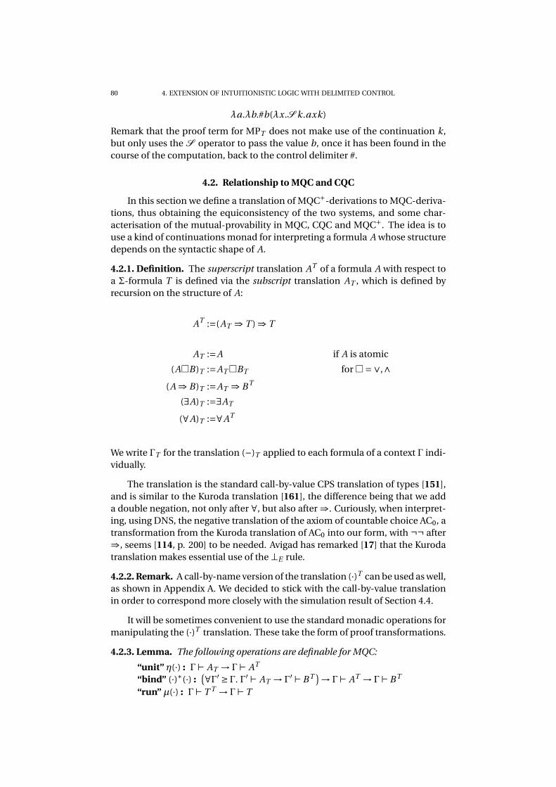
80 4. EXTENSION OF INTUITIONISTIC LOGIC WITH DELIMITED CONTROL
λa.λb.#b(λx.S k.axk)
Remark that the proof term for MPT does not make use of the continuation k,but only uses the S operator to pass the value b, once it has been found in thecourse of the computation, back to the control delimiter #.
4.2. Relationship to MQC and CQC
In this section we define a translation of MQC+-derivations to MQC-deriva-tions, thus obtaining the equiconsistency of the two systems, and some char-acterisation of the mutual-provability in MQC, CQC and MQC+. The idea is touse a kind of continuations monad for interpreting a formula A whose structuredepends on the syntactic shape of A.
4.2.1. Definition. The superscript translation AT of a formula A with respect toa Σ-formula T is defined via the subscript translation AT , which is defined byrecursion on the structure of A:
AT :=(AT ⇒ T ) ⇒ T
AT :=A if A is atomic
(A�B)T :=AT�BT for �=∨,∧
(A ⇒ B)T :=AT ⇒ B T
(∃A)T :=∃AT
(∀A)T :=∀AT
We write ΓT for the translation (−)T applied to each formula of a context Γ indi-vidually.
The translation is the standard call-by-value CPS translation of types [151],and is similar to the Kuroda translation [161], the difference being that we adda double negation, not only after ∀, but also after ⇒. Curiously, when interpret-ing, using DNS, the negative translation of the axiom of countable choice AC0, atransformation from the Kuroda translation of AC0 into our form, with ¬¬ after⇒, seems [114, p. 200] to be needed. Avigad has remarked [17] that the Kurodatranslation makes essential use of the ⊥E rule.
4.2.2. Remark. A call-by-name version of the translation (·)T can be used as well,as shown in Appendix A. We decided to stick with the call-by-value translationin order to correspond more closely with the simulation result of Section 4.4.
It will be sometimes convenient to use the standard monadic operations formanipulating the (·)T translation. These take the form of proof transformations.
4.2.3. Lemma. The following operations are definable for MQC:
“unit” η(·) : Γ⊢ AT → Γ⊢ AT
“bind” (·)∗(·) :(∀Γ′ ≥ Γ. Γ′ ⊢ AT → Γ
′ ⊢ B T)→ Γ⊢ AT → Γ⊢ B T
“run” µ(·) : Γ⊢ T T → Γ⊢ T

4.2. RELATIONSHIP TO MQC AND CQC 81
PROOF. Using the proof terms:
η=α 7→λk.kα
µ=α 7→α(λa.a)
φ∗q =λk.q(λa.(φ ·a)k)
�
Notice that we can only “run” a monad when it is of form T T and T is a Σ-formula.
We will denote derivation in MQC+by “⊢+”, derivation in MQC by “⊢m”,derivation in IQC by “⊢i ”, and the one in CQC by “⊢c ”.
4.2.4. Theorem (Equiconsistency). Given a derivation of Γ ⊢+ A, which uses S
and # for the Σ-formula T , we can build a derivation of ΓT ⊢m AT .
PROOF. By induction on the derivation. For each rule we use a correspond-ing proof term from the table below, except in the cases for ∧,∨,∃ – when theformula being proved is a Σ-formula – then we can simply apply the last usedderivation rule on the induction hypotheses.
a =λk.ka = η ·a
λa.p =λk.k(λa.λk ′.p
(λb.k ′b
))
pq =λk.p(λ f .q
(λa. f a (λb.kb)
))
(p, q) =λk.p(λa.q (λb.k (a,b))
)
π1p =λk.p (λc.k (π1c))
ι1p =λk.p (λa.k (ι1a))
case p of(a1.q1‖a2.q2
)=λk.p
(λc. case c of
(a1.q1k‖a2.q2k
))
λx.p =λk.k(λx.λk ′.p
(λb.k ′b
))
pt =λk.p(λ f . f tk
)
(t , p) =λk.p (λa.k(t , a))
dest p as (x.a) in q =λk.p(λc. dest c as (x.a) in qk
)
#ap =λk.k(p(λa.a)
)= η · (µ ·p)
S l .p =λk.(p(λa.a)
){λa.λk ′.k ′ (ka)
/l}
=λk.(µ ·p
){λa.η · (ka)
/l}
�
We would now like to compare the MQC+-provability of certain forms offormulae with their probability in MQC and CQC. Please note that we abuse thelanguage by taking CQC to be MQC plus the double-negation elimination rulerelative to a global fixed formula T i.e. ⊢c ¬T ¬T A →⊢c A. By ¬T A we denotethe formula A ⇒ T . When it is clear from the context, we omit the annotation T
from ¬T .
4.2.5. Definition. The Markov Principle for T is the following generalisation ofthe minimal-logic version of Markov’s principle:
(MPT ) (T ⇒ S) ⇒¬T ¬T S ⇒ S,
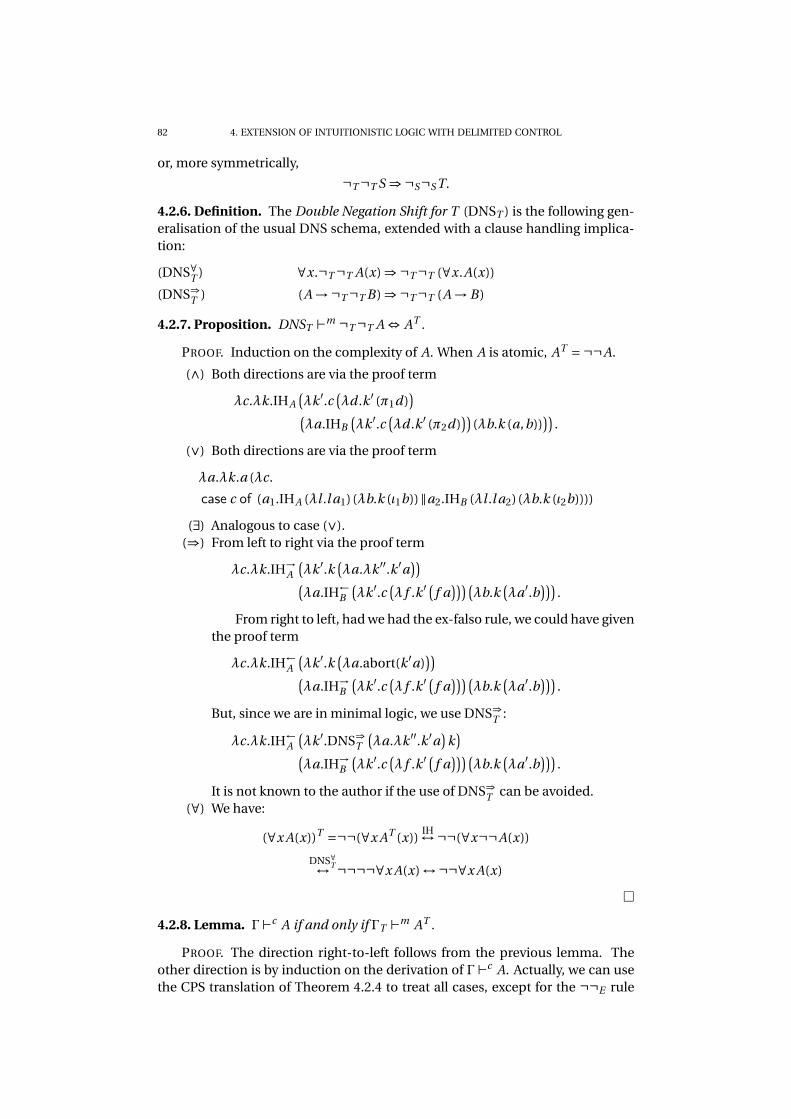
82 4. EXTENSION OF INTUITIONISTIC LOGIC WITH DELIMITED CONTROL
or, more symmetrically,
¬T ¬T S ⇒¬S¬ST.
4.2.6. Definition. The Double Negation Shift for T (DNST ) is the following gen-eralisation of the usual DNS schema, extended with a clause handling implica-tion:
∀x.¬T ¬T A(x) ⇒¬T ¬T (∀x.A(x))(DNS∀T )
(A →¬T ¬T B) ⇒¬T ¬T (A → B)(DNS⇒T )
4.2.7. Proposition. DNST ⊢m ¬T ¬T A ⇔ AT .
PROOF. Induction on the complexity of A. When A is atomic, AT =¬¬A.
(∧) Both directions are via the proof term
λc.λk.IHA
(λk ′.c
(λd .k ′ (π1d)
)(λa.IHB
(λk ′.c
(λd .k ′ (π2d)
))(λb.k (a,b))
)).
(∨) Both directions are via the proof term
λa.λk.a (λc.
case c of (a1.IHA (λl .l a1) (λb.k (ι1b))‖a2.IHB (λl .l a2) (λb.k (ι2b))))
(∃) Analogous to case (∨).(⇒) From left to right via the proof term
λc.λk.IH→A
(λk ′.k
(λa.λk ′′.k ′a
))(λa.IH←
B
(λk ′.c
(λ f .k ′
(f a
)))(λb.k
(λa′.b
))).
From right to left, had we had the ex-falso rule, we could have giventhe proof term
λc.λk.IH←A
(λk ′.k
(λa.abort(k ′a)
))(λa.IH→
B
(λk ′.c
(λ f .k ′
(f a
)))(λb.k
(λa′.b
))).
But, since we are in minimal logic, we use DNS⇒T :
λc.λk.IH←A
(λk ′.DNS⇒
T
(λa.λk ′′.k ′a
)k)
(λa.IH→
B
(λk ′.c
(λ f .k ′
(f a
)))(λb.k
(λa′.b
))).
It is not known to the author if the use of DNS⇒T can be avoided.
(∀) We have:
(∀x A(x))T =¬¬(∀x AT (x))IH↔¬¬(∀x¬¬A(x))
DNS∀T
↔ ¬¬¬¬∀x A(x) ↔¬¬∀x A(x)
�
4.2.8. Lemma. Γ⊢c A if and only if ΓT ⊢m AT .
PROOF. The direction right-to-left follows from the previous lemma. Theother direction is by induction on the derivation of Γ⊢c A. Actually, we can usethe CPS translation of Theorem 4.2.4 to treat all cases, except for the ¬¬E rule

4.3. SUBJECT REDUCTION AND PROGRESS 83
which was not covered by the translation. To show that ΓT ⊢m AT follows fromΓT ⊢m (¬¬A)T , we use the fact that ⊢m ¬¬(TT ) ↔ T (by the µ and η operators):
(¬¬A)T = ((A ⇒ T ) ⇒ T )T =¬¬((AT ⇒¬¬T ) ⇒¬¬T )
⇔¬¬((AT ⇒ T ) ⇒ T ) =¬¬¬¬AT ⇔¬¬AT = AT .
�
4.2.9. Corollary. For any formula A, we have:
⊢+ A4.2.4 // ⊢m AT
4.2.7��
oo 4.2.8 // ⊢c A
⊢+ ¬¬A DNST ⊢m ¬¬Aoo
4.2.10. Corollary. For any formula A, we have the following diagram:
⊢+ ¬¬A4.2.4 // ⊢m (¬¬A)T
4.2.7��
oo 4.2.8 // ⊢c A
DNST ⊢m ¬¬A
OO
DNST ⊢m ¬¬¬¬Aoo
In particular, the statement⊢+ ¬¬A ←→⊢c A represents an extension of Glivenko’s
theorem [81, 171, 181] to predicate logic.
4.3. Subject reduction and progress
In this section we prove that the reduction on proof terms satisfies SubjectReduction and Progress. First, a couple of lemmas are in order.
4.3.1. Lemma (Annotation Weakening). If Γ⊢ p : A, then Γ⊢T p : A for any T .
PROOF. A simple induction on the derivation. �
4.3.2. Lemma (Substitutions). The following hold:
(1) If Γ, a : A ⊢⋄ p : B and Γ⊢⋄ q : A, then Γ⊢⋄ p{q/a} : B.
(2) If Γ⊢⋄ p : B(x), where x is fresh, and t is a closed term, then Γ⊢⋄ p{t/x} :B(t ).
PROOF. The proof is standard, by induction on the derivation (see for exam-ple [155]). The new rules S and # pose no problems, since we can use the identi-ties (#p){q/a} = #(p{q/a}) and (S k.p){q/a} =S k.(p{q/a}) when k is fresh. �
4.3.3. Lemma (Decomposition). If Γ ⊢T P [S k.p] : B, then there is a formula A
and derivations Γ,k : A ⇒ T ⊢T p : T and Γ, a : A ⊢T P [a] : B.
PROOF. The proof is by induction on the derivation. We only need to con-sider the rules that can generate a pure evaluation context of the required form.Of the rules that we consider, for the intuitionistic rules, the proof is simply byusing the induction hypothesis, as shown below for the ∧I rule; and the onlynon-intuitionistic rule to consider is S , because # does not generate a pure eval-uation context.
• For ∧I , there are two cases to consider, depending on whether the pureevaluation context is (P [S k.p], q) or (V ,P [S k.p]), but the proofs areanalogous. Let the last rule in the derivation be:

84 4. EXTENSION OF INTUITIONISTIC LOGIC WITH DELIMITED CONTROL
Γ⊢T P [S k.p] : B1 Γ⊢T q : B2
Γ⊢T (P [S k.p], q) : B1 ∧B2
The induction hypothesis gives us a formula A1 and two derivations,Γ,k : A1 ⇒ T ⊢T p : T and Γ, a : A1 ⊢T P [a] : B1, from which the goalfollows by choosing A := A1.
• For S , the pure evaluation context must be the empty one, so the lastused rule is:
Γ,k : B ⇒ T ⊢T p : T
Γ⊢T [S k.p] : B
If we set A := B , the goal follows from the premise of the rule above and,for Γ, a : A ⊢T [a] : A, from the AX rule.
�
4.3.4. Lemma (Annotation Strengthening). Γ⊢S V : T −→ Γ⊢V : T
PROOF. The proof is by induction on the derivation and very simple. We onlyneed to consider the intuitionistic rules that introduce a value and that prove aΣ-formula, that is, the rules AX, ∧I , ∨1
I , ∨2I , and ∃I . S and # do not introduce a
value. �
4.3.5. Theorem (Subject Reduction). If Γ⊢⋄ p : A and p → q, then Γ⊢⋄ q : A.
PROOF. The proof is by induction on the derivation and is standard (see forexample [155]), by using Substitutions Lemma 4.3.2 and Decomposition Lemma4.3.3. Below, we consider the new rules and, for illustration, one of the intuition-istic rules.
(#) We have Γ ⊢⋄ #p and #p → q for some q . We look at three possiblecases, because there are three rules for rewriting a term of form #p. Ifq ≡ #q ′ and the reduction was by the congruence rule, we have p → q ′;now use IH and the # rule to finish the proof. If p is a value and q ≡ p,then Γ ⊢T q : T ; now use Strengthening Lemma 4.3.4 to conclude Γ ⊢
q : T . The third case is when p ≡ P [S k.p ′] and q ≡ #p ′{(λa.#P [a])/k},and the proof is by combining Lemmas 4.3.2 and 4.3.3.
(S ) This case is impossible, since there are no rules for reducing a termof form S k.p on its own, and the set of evaluation contexts does notinclude a clause for S k.[ ].
(∧1E ) We have Γ⊢⋄ p : A∧B , Γ⊢⋄ π1p : A, and π1p → q . If the reduction was
by the congruence rule, then q ≡ π1q ′ for some q ′, and we can use IH.Otherwise, p ≡ (V1,V2) and q ≡ V1, and Γ ⊢⋄ p : A ∧B must have beenproved by the ∧I rule, which is enough.
�
While the theorem above shows that reducing a proof term does not changeits logical specification, the next one shows that a proof term which is not innormal form does not get “stuck”.
4.3.6. Theorem (Progress). If ⊢⋄ p : A, p is not a value, and p is not of form
P [S k.p ′], then p reduces in one step to some proof term r .
PROOF. By induction on the derivation. The cases AX, (⇒I ), and (∀I ) intro-duce a value, while the case (S ) introduces a S k.p term.

4.4. NORMALISATION, DISJUNCTION AND EXISTENCE PROPERTIES 85
(∧I ) We have that ⊢⋄ (p, q) : A ∧B and (p, q) is neither a value nor of formP [S k.p ′]. Then also none of p, q is of form P [S k.p ′]. If p is not value,by IH, for some r , (p, q) → (r, q). If p is a value, then q must be a non-value, and then we use IH on q .
(∧1E ) We have that ⊢⋄ π1p : A and that π1p, hence p itself, is not of form
P [S k.p ′]. If p is a value, then it must be a pair (V1,V2), so π1(V1,V2) →V1. If p is not a value, we can use IH to obtain π1p →π1r for some r .
(∨I ) From ⊢⋄ ι1p : A ∨B and ι1p a non-value and not of form P [S k.p ′], wehave that p is not a value and not of that form, so we use IH to obtainan r such that p → r , hence ι1p → ι1r .
(∨E ) We have ⊢⋄ case p of(a1.p1‖a2.p2
): C . If p is a value, then it is of
form ιi V , therefore case ιi V of(a1.p1‖a2.p2
)→ pi {V /ai }. If p is of form
P [S k.p ′], then so is case p of(a1.p1‖a2.p2
). Otherwise, we use IH to
obtain an r such that case p of(a1.p1‖a2.p2
)→ case r of
(a1.p1‖a2.p2
).
(⇒E ) We have ⊢⋄ pq : B . If either p or q is of form P [S k.p ′], then so ispq . If p is a value, then it is of form λa.r ; if q is a value E [(λa.r )q] →E [r {q/a}]; if q is not a value, by IH, E [(λa.r )q] → E [(λa.r )q ′] for someq ′. Otherwise, by IH, p → r for some r , so pq → r q .
(∀E ) We have ⊢⋄ pt : A(t ). If p is of form P [S k.p ′], then so is pt . If p is avalue, then it is of form λx.r , hence (λx.r )t → r {t/x}. Otherwise, by IH,p → r for some r , so pt → r t .
(∃I ) From ⊢⋄ (t , p) : A(t ) and (t , p) a non-value and not of form P [S k.p ′],we have that p is not a value and not of that form, so we use IH to obtainan r such that (t , p) → (t ,r ).
(∃E ) We have ⊢⋄ dest p as (x.a) in q : C . If p is a value, then it is of form(t ,V ), therefore dest (t ,V ) as (x.a) in q → q {t/x} {V /a}. If p is of formP [S k.p ′], then so is dest p as (x.a) in q . Otherwise, we use IH to obtainan r such that dest p as (x.a) in q → dest r as (x.a) in q .
(#) We have ⊢⋄ #p : T . If p is a value, then #p → p. If p ≡ P [S k.p ′], then#p → #p ′{λa.#P [a]/k}. If p is neither a value nor of form P [S k.p ′], byIH, p → p ′, so #p → #p ′.
�
4.4. Normalisation, disjunction and existence properties
In this section we prove that every well-delimited4 proof term of MQC+,which is not a value, reduces to a value in finitely many steps.
A first approach would be to use Normalisation of MQC and Theorem 4.2.4,and prove in addition only that the CPS translation preserves reduction, that is,if ⊢+ p : A and p → r , then pk →+ r k, for any proof term k of the right type.For the case of simply-typed call-by-value lambda calculus, and a CPS trans-lation equivalent to ours, this statement is known as Plotkin’s simulation the-orem [151]. But, even for that restriction of our calculus (no pairs, no sums,and no delimited control), Plotkin had to come up with a technique known asthe “colon” translation, in order to deal with “administrative” η-redexes, and theoverall translation proceeds in two phases.
4By well-delimited, we will refer to proof terms in which there is an enclosing reset delimiterfor the shift operators used. That is, a proof term is well-delimited, when it corresponds to aderivation ⊢+ without an annotating Σ-formula at the root of the derivation tree.

86 4. EXTENSION OF INTUITIONISTIC LOGIC WITH DELIMITED CONTROL
Instead of extending the colon translation to the additional constructs thatwe have, we took the approach of Danvy and Filinski from [60]. They give aone-phase proof of simulation for the call-by-value lambda calculus that avoidsthe colon translation, and also shows how to handle the extra logical connec-tives and delimited control. The trick is to use a two-level lambda calculus: ameta-level consisting of the meta- function abstraction and application, and anobject-level lambda calculus as target of the translation. In that way, the admin-istrative η-redexes can be handled by the meta-language.
The two-level CPS translation is given in Table 3. The meta-level abstractionand application are denoted by “7→” and “α ·b”, to differ from the object levelones, “λ” and “ab”. The Greek letter κ will stand for meta-continuations, that is,proof transformations of type ΓT ⊢m AT → ΓT ⊢m T , and the letters α,β,γ,φ willstand for derivations ΓT ⊢m C . The meta-continuation “id” will stand for α 7→α.For the typing of the two-level translation of p we thus have
p : (ΓT ⊢m AT → ΓT ⊢m T ) → ΓT ⊢m T.
Note, however, that for the lemmas of this section to be well-typed, we need tobe slightly more general in the typing as described in Appendix A. The addedcomplexity does not change the argument, therefore we give a version whichcloselly follows the original work of Danvy and Filinski.
a = κ 7→ κ ·a
λa.p = κ 7→ κ ·(λa.λk.p ·
(β 7→ kβ
))
pq = κ 7→ p ·(φ 7→ q ·
(α 7→φα (λb.κ ·b)
))
(p, q) = κ 7→ p ·(α 7→ q ·
(β 7→ κ ·
(α,β
)))
π1p = κ 7→ p ·(γ 7→ κ ·
(π1γ
))
ι1p = κ 7→ p · (α 7→ κ · (ι1α))
case p of(a1.q1‖a2.q2
)= κ 7→ p ·
(γ 7→
(case γ of
(a1.q1 ·κ‖a2.q2 ·κ
)))
λx.p = κ 7→ κ ·(λx.λk.p ·
(β 7→ kxβ
))
pt = κ 7→ p ·(φ 7→φt (λb.κ ·b)
)
(t , p) = κ 7→ p · (α 7→ κ · (t ,α))
dest p as (x.a) in q = κ 7→ p ·(γ 7→
(dest γ as (x.a) in q ·κ
))
#p = κ 7→ κ ·(p · id
)
S l .p = κ 7→(p · id
){λa.λk.k (κ ·a)
/l}
Table 3: Two-level CPS translation
4.4.1. Lemma. If ⊢+ V : A for V a value, then, for any κ, we have that V ·κ =
κ · (V · id).
PROOF. We do induction on the derivation and consider only the rules thatcan introduce a value (Definition 4.1.3).
(AX) a ·κ= (κ 7→ κ ·a) ·κ= κ ·a = κ · ((κ 7→ κ ·a) · id) = κ · (a · id).

4.4. NORMALISATION, DISJUNCTION AND EXISTENCE PROPERTIES 87
(∧I )
(V1,V2) ·κ=V1 ·(α 7→V2 ·
(β 7→ κ ·
(α,β
)))
=V2 ·(β 7→ κ ·
(V1 · id,β
))
= κ ·(V1 · id,V2 · id
)
= κ ·(V2 ·
(β 7→
(V1 · id,β
)))
= κ ·(V1 ·
(α 7→V2 ·
(β 7→
(α,β
))))
= κ ·(V1 ·
(α 7→V2 ·
(β 7→ id ·
(α,β
))))= κ ·
((V1,V2) · id
)
(∨1I )
ι1V ·κ=V · (α 7→ κ · (ι1α))
= κ ·(ι1
(V · id
))
= κ ·(V · (α 7→ (ι1α))
)
= κ ·(V · (α 7→ id · (ι1α))
)= κ ·
(ι1V · id
)
(⇒I )
λa.p ·κ= κ ·(λa.λk.p ·
(β 7→ kβ
))
= κ ·(id ·
(λa.λk.p ·
(β 7→ kβ
)))= κ ·
(λa.p · id
)
The cases (∀I ) and (∃I ) are analogous to the ones of (⇒I ) and (∨1I ). �
4.4.2. Lemma. If Γ ⊢+ q : A and V is a closed value, then q{V /a} ·κ =(q ·κ
){V ·
id/a}, for any κ, a.
PROOF. By induction on the derivation of q .If Γ ⊢+ q : A is derived by the AX rule, then q is a variable. If q = a, then by
Lemma 4.4.1, a{V /a} ·κ = V ·κ = κ · (V · id) = (κ 7→ κ · (V · id)) ·κ = ((κ 7→ κ · a) ·κ){(V · id)/a} = (a ·κ){V · id/a}. Otherwise, V = b 6= a and the substitution has noeffect.
The rest of the cases are directly by the induction hypothesis, using the factthat V is closed and that the binders λ and S bind fresh variables, hence thesubstitution {V /a} can traverse the structure of q . We give one case for illustra-tion.
(S l .p
){V / a} ·κ=S l .
(p {V / a}
)·κ
=(p {V / a} · id
){λb.λk.k (κ ·b)
/l}
=(p · id
){V · id
/a}{
λb.λk.k (κ ·b)/
l}
=(p · id
){λb.λk.k (κ ·b)
/l}{
V · id/
a}
=S l .p{
V · id/
a}
�

88 4. EXTENSION OF INTUITIONISTIC LOGIC WITH DELIMITED CONTROL
4.4.3. Lemma. If P is a pure evaluation context, then, for every κ,
P [S l .s] ·κ=(s · id
){λa.λk.k(P [a] ·κ)/l
}.
PROOF. By induction on the derivation of P , considering only rules that canconstruct a pure evaluation context (Definition 4.1.4).
For the empty pure evaluation context [ ], the equality follows directly fromthe two-level CPS translation of S :
[S l .s] ·κ=(s · id
){λa.λk.k (κ ·a)
/l}
=(s · id
){λa.λk.k
([a] ·κ
)/l}
For the other cases, it is enough to show that Q[P [r ]] = P [r ] ·κ for some κ andany r . For example,
P [S l .s]q ·κ= P [S l .s] ·(φ 7→ q ·
(α 7→φα (λb.κ ·b)
))
=(s · id
){λa.λk.k
(P [a] ·
(φ 7→ q ·
(α 7→φα (λb.κ ·b)
)))/l}
=(s · id
){λa.λk.k
(P [a]q ·κ
)/l}
.
From the sole form of the two-level CPS, this follows for the cases P [S l .s]q ,
(P [S l .s], q), (V ,P [S l .s]), π1P [S l .s], ι1P [S l .s], case P [S l .s] of(a1.q1‖a2.q2
),
P [S l .s]t , (t ,P [S l .s]), and dest P [S l .s] as (x.a) in q . Hence we have to check
only(λa.p
)P [S l .s] (and
(λx.p
)P [S l .s] which is analogous):
(λa.p)P [r ] ·κ=λa.p ·(φ 7→ P [r ] ·
(α 7→φα (λb.κ ·b)
))
=(φ 7→ P [r ] ·
(α 7→φα (λb.κ ·b)
))·(λa.λk.s ·
(β 7→ kβ
))
= P [r ] ·(α 7→
(λa.λk.s ·
(β 7→ kβ
))α (λb.κ ·b)
)
�
4.4.4. Lemma. If V is a value, then so is V · id.
PROOF. By a simple induction on the derivation of V . We need to use Lemma4.4.1 for the case of ∧,∨ and ∃. �
The following lemma is a strengthening of Theorem 4.3.6 that, besides prov-ing that the proof term p reduces in one step to r in MQC+, proves also that itstwo-level CPS translation applied to a meta-continuation κ gives rise to:
• no reduction in MQC, when p → r by one of the two reduction rules forreset;
• at least one step of reduction in MQC, when p → r by normal weak-head reduction, that is, by a reduction rule which is not one for resetand not the congruence rule;
• the same number of reduction steps in MQC, as the number of steps bythe congruence rule.

4.4. NORMALISATION, DISJUNCTION AND EXISTENCE PROPERTIES 89
We will use the wild-card notation →⋄ to denote this dependency of thenumber of reduction steps for the translation, on the sort of the reduction ruleused in MQC+. We also use the wildcard for the Σ-formula annotation of ⊢+, butthe two uses of the wildcard are of course not related.
4.4.5. Lemma (CPS-Progress). If ⊢+⋄ p : A, p is not a value, and p is not of form
P [S k.p ′], then, for some r , p →1 r and, for any κ, p ·κ→⋄ r ·κ.
PROOF. The proof has the same structure as the one of Theorem 4.3.6, there-fore we will just amend it with the part concerning the two-level CPS translation.
(∧I ) We consider the pair (p, q). If p → r , then (p, q) ·κ = p · (α 7→ q · (β 7→
κ · (α,β)))IH→⋄ r · (α 7→ q · (β 7→ κ · (α,β))) = (r, q) ·κ.
If p is a value and q → r , then (p, q)·κ= p ·(α 7→ q ·(β 7→ κ·(α,β)))IH→⋄
p · (α 7→ r · (β 7→ κ · (α,β))) = (p,r ) ·κ.(∧1
E ) We consider the termπ1p. If p is a value, it is a pair (V1,V2) andπ1(V1,V2) →V1. Then, by using Lemma 4.4.1 and Lemma 4.4.4,
π1(V1,V2) ·κ= (V1,V2) · (γ 7→ κ · (π1γ))
=V1 ·(α 7→V2 ·
(β 7→
(γ 7→ κ ·
(π1γ
))·(α,β
)))
=V2 ·(β 7→
(γ 7→ κ ·
(π1γ
))·(V1 · id,β
))
=(γ 7→ κ ·
(π1γ
))·(V1 · id,V2 · id
)
= κ ·(π1
(V1 · id,V2 · id
))
→ κ ·(V1 · id
)
=V1 ·κ.
If p is not a value, then π1p →π1r for some r , and
π1p ·κ= p · (γ 7→ κ · (π1γ))
IH→⋄ r · (γ 7→ κ · (π1γ))
=π1r ·κ.
(∨I ) We need to consider ι1p when p is neither a value nor of form P [S k.p ′],and when there is an r such that p → r .
ι1p ·κ= p · (α 7→ κ · (ι1α))
IH→⋄ r · (α 7→ κ · (ι1α))
= ι1r ·κ.
(∨E ) We consider case p of(a1.q1‖a2.q2
). If p is a value, we know that
case ιi V of(a1.q1‖a2.q2
)→ qi {V /ai },

90 4. EXTENSION OF INTUITIONISTIC LOGIC WITH DELIMITED CONTROL
and then, by using Lemma 4.4.1, Lemma 4.4.2 and Lemma 4.4.4,
case ιi V of(a1.q1‖a2.q2
)·κ= ιi V ·
(γ 7→
(case γ of
(a1.q1 ·κ‖a2.q2 ·κ
)))
=V ·(α 7→
(γ 7→
(case γ of
(a1.q1 ·κ‖a2.q2 ·κ
)))· (ιiα)
)
=V ·(α 7→
(case ιiα of
(a1.q1 ·κ‖a2.q2 ·κ
)))
=(case ιi
(V · id
)of
(a1.q1 ·κ‖a2.q2 ·κ
))
→ (qi ·κ){V · id/ai }
= qi {V /ai } ·κ.
Otherwise, p → r for some r , and
case p of(a1.q1‖a2.q2
)·κ= p ·
(γ 7→
(case γ of
(a1.q1 ·κ‖a2.q2 ·κ
)))
IH→⋄ r ·
(γ 7→
(case γ of
(a1.q1 ·κ‖a2.q2 ·κ
)))
= case r of(a1.q1‖a2.q2
)·κ.
(⇒E ) We consider the proof term pq . If p and q are both values, then p =
λa.s and pq → s{q/a}. Then, by using Lemma 4.4.1 and Lemma 4.4.2,
(λa.s)q ·κ=λa.s ·(φ 7→ q ·
(α 7→φα (λb.κ ·b)
))
=(φ 7→ q ·
(α 7→φα (λb.κ ·b)
))·(λa.λk.s · (b 7→ kb)
)
= q ·(α 7→
(λa.λk.s · (b 7→ kb)
)α (λb.κ ·b)
)
→+ q ·(α 7→
(s · (b 7→ κ ·b)
){α/a}
)
= q ·(α 7→
(s ·κ
){α/a}
)
= (s ·κ){q · id/a}
= s{q/a} ·κ.
In the →+ step we used the fact that s can have at most a as free vari-able, which follows from p =λa.s being a closed term.
If p is a value λa.s and q is not, then q → r for some r , and
(λa.s)q ·κ=λa.s ·(φ 7→ q ·
(α 7→φα (λb.κ ·b)
))
→⋄ λa.s ·(φ 7→ r ·
(α 7→φα (λb.κ ·b)
))
= (λa.s)r ·κ.
Otherwise, when p is not a value, and p → r for some r , we havethat
pq ·κ= p ·(φ 7→ q ·
(α 7→φα (λb.κ ·b)
))
→⋄ r ·(φ 7→ q ·
(α 7→φα (λb.κ ·b)
))
= r q ·κ.
(∀E ) By analogy with ⇒E , but simpler.(∃I ) By analogy with ∨I .(∃E ) By analogy with ∨E .
(#) We consider the proof term #p. If p is a value, then #p → p and
#p ·κ= κ · (p · id) = p ·κ.
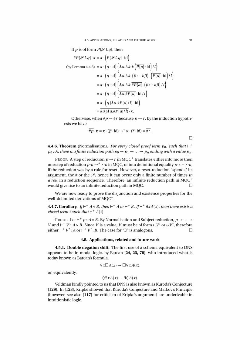
4.5. APPLICATIONS, RELATED AND FUTURE WORK 91
If p is of form P [S l .q], then
#P [S l .q] ·κ= κ ·(P [S l .q] · id
)
(by Lemma 4.4.3) = κ ·(q · id
){λa.λk.k
(P [a] · id
)/l
}
= κ ·(q · id
){λa.λk.
(β 7→ kβ
)·(P [a] · id
)/l
}
= κ ·(q · id
){λa.λk.#P [a] ·
(β 7→ kβ
)/l
}
= κ ·(q · id
){λa.#P [a] · id/l
}
= κ ·(q {λa.#P [a]/l } · id
)
= #q {λa.#P [a]/l } ·κ.
Otherwise, when #p → #r because p → r , by the induction hypoth-esis we have
#p ·κ= κ · (p · id) →⋄ κ · (r · id) = #r .
�
4.4.6. Theorem (Normalisation). For every closed proof term p0, such that ⊢+
p0 : A, there is a finite reduction path p0 → p1 → . . . → pn ending with a value pn .
PROOF. A step of reduction p → r in MQC+ translates either into more thenone step of reduction p ·κ→+ r ·κ in MQC, or into definitional equality p ·κ= r ·κ,if the reduction was by a rule for reset. However, a reset-reduction “spends” itsargument, the # or the S , hence it can occur only a finite number of times in
a row in a reduction sequence. Therefore, an infinite reduction path in MQC+
would give rise to an infinite reduction path in MQC. �
We are now ready to prove the disjunction and existence properties for thewell-delimited derivations of MQC+.
4.4.7. Corollary. If ⊢+ A∨B, then ⊢+ A or ⊢+ B. If ⊢+ ∃x A(x), then there exists a
closed term t such that ⊢+ A(t ).
PROOF. Let ⊢+ p : A∨B . By Normalisation and Subject reduction, p →···→
V and ⊢+ V : A∨B . Since V is a value, V must be of form ι1V ′ or ι2V ′, thereforeeither ⊢+ V ′ : A or ⊢+ V ′ : B . The case for “∃” is analogous. �
4.5. Applications, related and future work
4.5.1. Double negation shift. The first use of a schema equivalent to DNSappears to be in modal logic, by Barcan [24, 23, 78], who introduced what istoday known as Barcan’s formula,
∀x�A(x) →�∀x A(x),
or, equivalently,♦∃x A(x) →∃♦A(x).
Veldman kindly pointed to us that DNS is also known as Kuroda’s Conjecture[129]. In [123], Kripke showed that Kuroda’s Conjecture and Markov’s Principle(however, see also [117] for criticism of Kripke’s argument) are underivable inintuitionistic logic.

92 4. EXTENSION OF INTUITIONISTIC LOGIC WITH DELIMITED CONTROL
In [118, Section 2.11], Kreisel used the principle
(GMP) ¬∀n A(n) ⇒∃n¬A(n),
for A(n) an arbitrary formula, to deal with implication while giving a transla-tion of formulae of Analysis into functionals of finite type. In [148], Oliva callsthis principle the Generalised Markov Principle and remarks that HAω ⊢ DNS ↔
¬¬GMP. Kreisel does not give a justification of GMP in his paper.The term “double negation shift” appears for the first time in [157] to denote
the formula
(DNS) ∀n¬¬A(n) ⇒¬¬∀n A(n).
There, Spector builds upon previous works of Gödel [88, 89, 90], namely he re-alises DNS by adding the schema of bar recursion to Gödel’s system T. The name“bar recursion” comes from the Bar Principle of Brouwer which is used in jus-tifying it. However, Spector attaches no particular interest to the DNS schemaitself; he writes:
The schema [DNS] is chosen not because we believe it is ofintuitionistic significance, but to provide a formal system inwhich classical analysis is easily interpreted, and whose logi-cal basis is intuitionistic.[157]
We treat DNS at the level of predicate logic, not of arithmetic, and we hopeto explore in the future the status of this change.
4.5.2. Negative translation of Countable Choice. The Axiom of CountableChoice is,
(AC0) ∀x0∃yρ A(x, y) ⇒∃ f 0→ρ∀x0 A(x, f (x)),
a formula schema of HAω, Heyting Arithmetic in all finite types. The type 0stands for the set of natural numbers N, the type 1 = 0 → 0 stands for the func-tions N→N, 2 stands for the functionals (0 → 0) → 0, and so on. Spector showedthat the Kuroda [114, p.163] negative translation, ¬¬(AC0
∗), of AC0,
(ACN0 ) ∀x0¬¬∃yρ A∗(x, y) ⇒∃ f 0→ρ∀x0¬¬A∗(x, f (x)),
is provable from DNS and the intuitionistic AC0. Since AC0 is realisable in HAω,and DNS is realisable by bar recursion, so is ACN
0 . His approach was extended toDependent Choice (DC) by Luckhardt [132] and Howard [106]. In recent years,Kohlenbach, Berger, and Oliva gave their own versions of bar recursion (see [30]for a comparison).
Since we treat DNS at the level of logic, we are only able to give an open proofterm deriving the negative translation of AC0,
(AC0T ) ∀x0¬T ¬T ∃yρ AT (x, y) ⇒¬T ¬T ∃ f 0→ρ∀x0¬T ¬T AT (x, f (x)).
Given a variable c to denote a proof of the intuitionistic AC0, we can use aproof term similar to the one of DNST for deriving the above schema:
λa.λk.#k(c(λx.S k ′.ax(λd .k ′(νd)))),
where ν is a proof term for ∃y AT (x, y) ⇒∃y AT (x, y).The proof term being open means that we can not immediately use it for
computation. We would have to either develop a realisability semantics for MQC+,
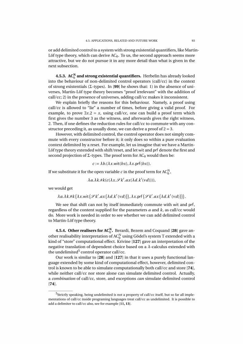
4.5. APPLICATIONS, RELATED AND FUTURE WORK 93
or add delimited control to a system with strong existential quantifiers, like Martin-Löf type theory, which can derive AC0. To us, the second approach seems moreattractive, but we do not pursue it in any more detail than what is given in thenext subsection.
4.5.3. ACN0 and strong existential quantifiers. Herbelin has already looked
into the behaviour of non-delimited control operators (call/cc) in the contextof strong existentials (Σ-types). In [99] he shows that: 1) in the absence of uni-verses, Martin-Löf type theory becomes “proof irrelevant” with the addition ofcall/cc; 2) in the presence of universes, adding call/cc makes it inconsistent.
We explain briefly the reasons for this behaviour. Namely, a proof usingcall/cc is allowed to “lie” a number of times, before giving a valid proof. Forexample, to prove ∃x.2 = x, using call/cc, one can build a proof term whichfirst gives the number 3 as the witness, and afterwards gives the right witness,2. Then, if one defines the reduction rules for call/cc to commute with any con-structor preceding it, as usually done, we can derive a proof of 2 = 3.
However, with delimited control, the control operator does not simply com-mute with every constructor before it; it only does so within a pure evaluationcontext delimited by a reset. For example, let us imagine that we have a Martin-Löf type theory extended with shift/reset, and let wit and prf denote the first andsecond projection of Σ-types. The proof term for AC0 would then be:
c :=λb.(λx.wit(bx),λx.prf(bx)).
If we substitute it for the open variable c in the proof term for ACN0 ,
λa.λk.#k(c(λx.S k ′.ax(λd .k ′(νd)))),
we would get
λa.λk.#k(λx.wit
(S k ′.ax
(λd .k ′ (νd)
)),λx.prf
(S k ′.ax
(λd .k ′ (νd)
))).
We see that shift can not by itself immediately commute with wit and prf,regardless of the content supplied for the parameters a and k, as call/cc woulddo. More work is needed in order to see whether we can add delimited controlto Martin-Löf type theory.
4.5.4. Other realisers for ACN0 . Berardi, Bezem and Coquand [28] gave an-
other realisability interpretation of ACN0 using Gödel’s system T extended with a
kind of “store” computational effect. Krivine [127] gave an interpretation of thenegative translation of dependent choice based on a λ-calculus extended withthe undelimited5 control operator call/cc.
Our work is similar to [28] and [127] in that it uses a purely functional lan-guage extended by some kind of computational effect, however, delimited con-trol is known to be able to simulate computationally both call/cc and store [74],while neither call/cc nor store alone can simulate delimited control. Actually,a combination of call/cc, store, and exceptions can simulate delimited control[74].
5Strictly speaking, being undelimited is not a property of call/cc itself, but so far all imple-mentations of call/cc inside programing languages treat call/cc as undelimited. It is possible toadd a delimiter to call/cc also, see for example [11, 13].
94 4. EXTENSION OF INTUITIONISTIC LOGIC WITH DELIMITED CONTROL
4.5.5. Negative translation of Dependent Choice. We mentioned that theapproach of Spector had been extended to handling the negative translation ofthe schema of Dependent Choice,
(DC) ∀x0∀yρ∃zρ .A(x, y, z) ⇒∃ f 0→ρ∀x0 A(x, f x, f (x +1)).
An axiom schema similar in shape to DNS is used for this purpose (see [114,p.208]),
∀x0∀cρ¬¬∃aρ∀bτA0(x,c, a,b) ⇒¬¬∃u0→ρ∀y0∀vτA0(y,uy,u(y +1), v),
where A0 is a decidable formula. We have not yet pursued the goal of treatingthis schema in our system.
4.5.6. Fan Theorem. Another attractive direction for further work concernsprinciples arising form Brouwer’s Bar Principle. It is folklore that all practicalconsequences of the Bar Principle are already consequences of the Fan Princi-ple,
(FAN) ∀α1∃n0 A0(αn) ⇒∃N 0∀α1∃n ≤ N .A0(αn),
where A0(x, y) is a decidable formula, and αn denotes the initial segment oflength n of the infinite stream α.
We started to work on giving a proof term for FAN, but due to lack of time wehad to stop. Our approach was to restate FAN, so that the right hand side of theimplication becomes a Σ-formula:
(FAN’) ∀α1∃n0 A0(αn) ⇒∃N 0∀m0 < 2N∃n ≤ N .A0(mn),
where mn turns a natural number m into its binary representation, appendingzeros to it if the binary representation has less than n bits. Since the internalquantification over α is bounded, we can work in a bounded arithmetic systemlike G3 Aω
i(which is strong enough to encode variable-length finite sequences
[114, p.54]) and consider the right-hand side of the implication as a Σ-formula.Bauer [26] reported to have used, together with Pretnar, delimited control to
give an alternative implementation of Escardó’s fan functional [65] for exhaus-tive search of Cantor space.
4.5.7. Open Induction and Bar Induction. In the context of IntuitionisticReverse Mathematics, Veldman considered the relationship between various in-tuitionistic principles [177, 176]. In particular, he recovered a result of Moschovakisand Solovay [142], that
BI+MP ⊢ DNS.
Besides other equivalences, he also connected the Open Induction Principle[50] on Cantor space (OI(C )) to the DNS schema.
Definition (OI(C )). For any U open subspace of Cantor space 2N and < the lex-icographical order on 2N, if
∀α.(∀β<α.β ∈U ) →α ∈U
then
∀α.α ∈U .

4.5. APPLICATIONS, RELATED AND FUTURE WORK 95
He shows thatMP ⊢ DNS ⇔ OI(C ),
henceDNS+MP ⇔ OI(C )+MP,
and also that FAN is strictly weaker than OI(C ), by giving a proof from OI(C ) ofthe Paris-Harrington theorem [150], which is independent of HA, while it wasestablished by Troelstra [160] that FAN is conservative over HA.
4.5.8. Shift and reset. The shift/reset delimited control operators have beenintroduced in [58, 59]. The purpose for introducing them was to exploit the ex-pressive power beyond the traditional CPS translation [151]; traditionally, pro-grams written in continuation passing style are of a specific form, all functionapplications calls are tail applications, but one can write programs in CPS thatmake non necessarily tail calls6, and then the question arises what are the origi-nal direct style operators that are translated into this extended-CPS form. Danvyand Filinski’s answer is shift/reset. They also generalise this procedure, makinga CPS translation of the already extended-CPS translated terms, and get a hierar-chy of shiftn/resetn operators, level n corresponding to the n-th extended-CPStranslation.
A typing system (known as “type-and-effect” system) for shift/reset appearsalready in [58], but it is difficult to connect to traditional logic because impli-cation is a quaternary not a binary connective. A typing system which is a spe-cialisation of Danvy-Filinski’s, but again has a ternary implication connective,appears in [144]. In his paper on simulating monadic effects [73], Filinski usesa typing system similar to ours, where implication is binary and the answer typeT is fixed.
Our work is different in that we look at the typing system in the context oflogic, with all usual connectives, not in the context of programming languages.Also, our proofs of subject reduction and progress are direct, while for Murthy’sand Filinski’s system these properties follow [35] from the embedding in Danvy-Filinski’s system.
Asai-Kameyama [14] revisit the type-and-effect system of Danvy-Filinski andextend it to a polymorphic one. Kiselyov-Shan give a typing system expressinga sub-structural logic, and small-step operational semantics (we give a big-stepsemantics) for shift/reset. Zeilberger[186] investigates delimited control in thecontext of polarised linear logic. Munch-Maccagnoni connects delimited con-trol to co-dereliction of differential linear logic. This list of related work refer-ences is far from exhaustive.
4.5.9. Felleisen’s control/prompt delimited control operators. There is avariety of delimited control operators in the programming languages literature.One of the earliest ones are Felleisen’s control (F ) and prompt (#). Their de-velopment was not motivated by the study of the extended CPS translation, butdirectly by the programming need of being able to compose continuations likeany other first class object inside a programing language (Scheme). The rela-tionship between control/prompt and shift/reset has been studied by many au-thors. Although shift/reset and control/prompt are mutually interpretable, and
6Indeed, the completeness proof of Chapter 3 uses non-tail calls in the case of disjunction.
96 4. EXTENSION OF INTUITIONISTIC LOGIC WITH DELIMITED CONTROL
their big-step operational semantics is quite similar,
#P [S k.p] → #p {(λa.#P [a])/k}
#P [Fk.p] → #p {(λa.P [a])/k} ,
operationally they behave differently: while shift sets a new control delimiteraround its former pure evaluation context, control does not. The PhD thesis ofBiernacki [35] contains a thorough comparison of shift and control, and furtherreferences.
In connection to MQC+, we have tried to check all the proofs with havingF instead of S . While most of the time the difference does not matter, in thesubject reduction theorem, when using control, we do not have to carry out aweakening step as with shift, but for the normalisation theorem it is not clearwhich two-level CPS translation to take if we had control instead of shift.
4.5.10. Herbelin’s calculus for Markov Principle. In [100], Herbelin presentsIQCMP, an intuitionistic calculus that derives Markov’s Principle. The calculusMQC+ that we present here has been derived starting from Herbelin’s calculus.There are two big differences between the two:
(1) Derivations of IQCMP are annotated by a context of Σ-formula, not justone formula. This permits, for example, to have a derivation which usesmultiple and different instances of Markov’s Principle.
We had also tried to have a version of MQC+ with context anno-tations, but encountered a problem with the CPS translation. Namely,when multiple Σ-formula annotations are present, one has to have auniform way to compose the monadsΓS ⊢ AS ,ΓT ⊢ AT , . . . indexed withdifferent Σ-formulae S,T, . . .. We hope to address this problem in thefuture.
(2) The second difference with IQCMP is in the rules for the delimited con-trol operators:
Γ⊢α:T,∆ p : TCATCH
Γ⊢∆ catchαp : T
Γ⊢∆ p : T (α : T ) ∈∆THROW
Γ⊢∆ throwαp : A
While catch is just #, the proof term throw p is a particular case ofS k.p that does not use the continuation k inside p.
Note that if we had context- and not single-formula-annotations for MQC+,then we would have the following characterisation of provability of Σ-formulasS:
⊢+ S4.2.4 //
⊢i S⊥
by def. of (·)⊥
oo 4.2.8 // ⊢c S
MP⊥ ⊢i S
OO
⊢i ¬¬Soo
4.5.11. Completeness for standard Kripke models. We started to investi-gate the logical meaning of delimited control because of Danvy’s program ofSection 3.2, that is, because of the possibility of a constructive completenessproof for full intuitionistic logic and standard Kripke semantics.
May we now close the circle and use MQC+to give such a proof? We believethat further work is necessary: 1) on having multipleΣ-formula annotations, like

4.5. APPLICATIONS, RELATED AND FUTURE WORK 97
in the system of Herbelin described in Subsection 4.5.10; 2) on allowing a certaindegree of “polymorphism” in the rules for shift and reset.
If we go back to the the algorithm of page 63, we see that, in a completenessproof having as base the given algorithm, the reset in the implication-reificationcase would be used for the Σ-formula
∃q. Γ, a : τ⊢ q : σ,
and shift would be used for a Σ-formula of the same form, ∃r. Γ ⊢ r : ρ, whichmeans that the continuation bound by the shift would have the type
κ : ∀Γ′ ≥ Γ.(Γ′ σ or Γ′ τ→∃r. Γ′ ⊢ r : ρ
).
Note that it is not possible to use the simpler typing of κ,
κ : Γ σ or Γ τ→∃r. Γ⊢ r : ρ,
because the continuation is applied in two contexts, inside the ❝❛s❡ expression,that are enriched by a1 and a2; the reset-s are there applied for the Σ-formulae
∃r. Γ, a1 : τ⊢ r : ρ and ∃r. Γ, a2 : σ⊢ r : ρ.
Then, it is clear that the shape of the formula that completeness (or reifica-tion) is applied to, determines how many Σ-formulae we would need to anno-tate our derivations with. It is also clear that we have to account somehow forthe polymorphic behaviour of the contexts. We thus propose the following rulesfor a future extension of MQC+,
Γ⊢(α:T ),∆ p : T (w,φ)#α
Γ⊢∆ #αp : T (w,φ)
Γ,k : ∀w ′ ≥ w.A(w ′,φ) ⇒ T (w ′,φ) ⊢∆ p : T (w,φ) (α : T (w,φ)) ∈∆Sα,
Γ⊢∆ Sαkp : A(w,φ)
which would be able to prove completeness for standard Kripke models if we letT (w,φ) encode intuitionistic provability of formulaφ in the context w , T (w,φ) :=∃n. pw ⊢ n : σq, and let A(w,φ) represent Kripke-validity of formula φ in thecontext w , A(w,φ) := w φ.
If the preorder between the individuals is to be avoided, we could use itsdefinability from page 70, to replace
k : ∀w ′ ≥ w.A(w ′,φ) ⇒ T (w ′,φ)
byk : ∀w ′.
[∀ψ.T (w,ψ) ⇒ T (w ′,ψ)
]⇒ A(w ′,φ) ⇒ T (w ′,φ).
4.5.12. Normalisation-by-evaluation for MQC+. The pass to the 2-level λ-calculus in order to give a simpler proof of reduction-preservation by the CPStranslation, indicates that there should be an NBE algorithm behind, which wouldexpress the normalisation proof in two distinct phases (reflection and reifica-tion). In future, we hope to be able to develop such a proof, by modifying thenotion of model from Chapter 3.
A work-in-progress towards an NBE program for shift/reset has been pre-sented in [166].
4.5.13. Monadic computational effects. Finally, we would like to see whatspecific monadic effects look like when expressed in a direct way, using shift/reset,in our system. The PhD thesis of Filinski [74] is a guide on how to do that.

Bibliography
[1] Proceedings, Sixth Annual IEEE Symposium on Logic in Computer Science, 15-18 July, 1991,
Amsterdam, The Netherlands. IEEE Computer Society, 1991.[2] 22nd IEEE Symposium on Logic in Computer Science (LICS 2007), 10-12 July 2007, Wroclaw,
Poland, Proceedings. IEEE Computer Society, 2007.[3] Andreas Abel. Weak beta-theta-normalization and normalization by evaluation for system
F. In Cervesato et al. [45], pages 497–511.[4] Andreas Abel. Typed applicative structures and normalization by evaluation for system Fω.
In Grädel and Kahle [91], pages 40–54.[5] Andreas Abel. Towards normalization by evaluation for the beta-eta-calculus of construc-
tions. In Blume et al. [36], pages 224–239.[6] Andreas Abel, Klaus Aehlig, and Peter Dybjer. Normalization by evaluation for Martin-Löf
type theory with one universe. Electr. Notes Theor. Comput. Sci., 173:17–39, 2007.[7] Andreas Abel, Thierry Coquand, and Peter Dybjer. Normalization by evaluation for Martin-
Löf type theory with typed equality judgements. In LICS [2], pages 3–12.[8] Andreas Abel, Thierry Coquand, and Peter Dybjer. Normalization by evaluation for Martin-
Löf type theory with typed equality judgements. In LICS [2], pages 3–12.[9] Andreas Abel, Thierry Coquand, and Peter Dybjer. Verifying a semantic beta-eta-conversion
test for Martin-Löf type theory. In Audebaud and Paulin-Mohring [15], pages 29–56.[10] Thorsten Altenkirch, Peter Dybjer, Martin Hofmann, and Philip J. Scott. Normalization by
evaluation for typed lambda calculus with coproducts. In LICS, pages 303–310, 2001.[11] Zena M. Ariola and Hugo Herbelin. Minimal classical logic and control operators. In Thirti-
eth International Colloquium on Automata, Languages and Programming, ICALP ’03, Eind-
hoven, The Netherlands, June 30 - July 4, 2003, volume 2719 of Lecture Notes in Computer
Science, pages 871–885. Springer, 2003.[12] Zena M. Ariola and Hugo Herbelin. Control reduction theories: the benefit of structural
substitution. J. Funct. Program., 18(3):373–419, 2008.[13] Zena M. Ariola, Hugo Herbelin, and Amr Sabry. A type-theoretic foundation of delimited
continuations. Higher Order and Symbolic Computation, 22(3):233–273, September 2009.online from 2007.
[14] Kenichi Asai and Yukiyoshi Kameyama. Polymorphic delimited continuations. In APLAS,pages 239–254, 2007.
[15] Philippe Audebaud and Christine Paulin-Mohring, editors. Mathematics of Program Con-
struction, 9th International Conference, MPC 2008, Marseille, France, July 15-18, 2008. Pro-
ceedings, volume 5133 of Lecture Notes in Computer Science. Springer, 2008.[16] Jeremy Avigad. Algebraic proofs of cut elimination. J. Log. Algebr. Program., 49(1-2):15–30,
2001.[17] Jeremy Avigad. A variant of the double-negation translation. Technical report, Carnegie
Mellon University, 2006. Technical Report CMU-PHIL 179.[18] Brian E. Aydemir, Arthur Charguéraud, Benjamin C. Pierce, Randy Pollack, and Stephanie
Weirich. Engineering formal metatheory. In Necula and Wadler [145], pages 3–15.[19] Vincent Balat. Une étude des sommes fortes : isomorphismes et formes normales. PhD thesis,
Université Paris 7, 2002.[20] Vincent Balat. Keeping sums under control, 2004.[21] Vincent Balat. Ocaml implementation of tdpe for sums, 2004.[22] Vincent Balat, Roberto Di Cosmo, and Marcelo P. Fiore. Extensional normalisation and type-
directed partial evaluation for typed lambda calculus with sums. In Jones and Leroy [110],pages 64–76.
99
100 BIBLIOGRAPHY
[23] Ruth C. Barcan. The deduction theorem in a functional calculus of first order based on strictimplication. The Journal of Symbolic Logic, 11(4):115–118, 1946.
[24] Ruth C. Barcan. A functional calculus of first order based on strict implication. The Journal
of Symbolic Logic, 11(1):1–16, 1946.[25] Freiric Barral. Exceptional nbe for sums. In Olivier Danvy, editor, Informal proceedings of the
2009 Workshop on Normalization by Evaluation, August 15th 2009, Los Angeles, California,pages 21–30, 2009.
[26] Andrej Bauer. personal communication, March 2010.[27] Arnold Beckmann, Ulrich Berger, Benedikt Löwe, and John V. Tucker, editors. Logical Ap-
proaches to Computational Barriers, Second Conference on Computability in Europe, CiE
2006, Swansea, UK, June 30-July 5, 2006, Proceedings, volume 3988 of Lecture Notes in Com-
puter Science. Springer, 2006.[28] Stefano Berardi, Marc Bezem, and Thierry Coquand. On the computational content of the
axiom of choice. J. Symbolic Logic, 63(2):600–622, 1998.[29] Stefano Berardi and Silvio Valentini. Krivine’s intuitionistic proof of classical completeness
(for countable languages). Ann. Pure Appl. Logic, 129(1-3):93–106, 2004.[30] U. Berger and P. Oliva. Modified bar recursion and classical dependent choice. In M. Baaz,
S.D. Friedman, and J. Kraijcek, editors, Logic Colloquium ’01, Proceedings of the Annual
European Summer Meeting of the Association for Symbolic Logic, held in Vienna, Austria,
August 6 - 11, 2001, volume 20 of Lecture Notes in Logic, pages 89–107. Springer, 2005.[31] Ulrich Berger. A computational interpretation of open induction. In F. Titsworth, editor,
Proceedings of the Ninetenth Annual IEEE Symposium on Logic in Computer Science, pages326–334. IEEE Computer Society, 2004.
[32] Ulrich Berger, Stefan Berghofer, Pierre Letouzey, and Helmut Schwichtenberg. Program ex-traction from normalization proofs. In Typed Lambda Calculi and Applications, number 664
in Lecture Notes in Computer Science, pages 91–106. Springer Verlag, 1993.[33] Ulrich Berger and Helmut Schwichtenberg. An inverse of the evaluation functional for
typed lambda-calculus. In LICS [1], pages 203–211.[34] Paul Bernays. Axiomatische untersuchung des aussagen-kalkuls der principia mathemat-
ica. Mathematische Zeitschrift, (25):305–320, 1926.[35] Dariusz Biernacki. The Theory and Practice of Programming Languages with Delimited Con-
tinuations. PhD thesis, DAIMI, Department of Computer Science, University of Aarhus,Denmark, 12 2005. BRICS DS-05-08.
[36] Matthias Blume, Naoki Kobayashi, and Germán Vidal, editors. Functional and Logic Pro-
gramming, 10th International Symposium, FLOPS 2010, Sendai, Japan, April 19-21, 2010.
Proceedings, volume 6009 of Lecture Notes in Computer Science. Springer, 2010.[37] Patrick Braselmann and Peter Koepke. Coincidence lemma and substitution lemma. For-
malized Mathematics, 13(1):17–26, 2005.[38] Patrick Braselmann and Peter Koepke. Consequences of the sequent calculus. Formalized
Mathematics, 13(1):41–44, 2005.[39] Patrick Braselmann and Peter Koepke. Equivalences of inconsistency and Henkin models.
Formalized Mathematics, 13(1):45–48, 2005.[40] Patrick Braselmann and Peter Koepke. Gödel’s completeness theorem. Formalized Mathe-
matics, 13(1):49–53, 2005.[41] Patrick Braselmann and Peter Koepke. A sequent calculus for first-order logic. Formalized
Mathematics, 13(1):33–39, 2005.[42] Patrick Braselmann and Peter Koepke. Substitution in first-order formulas: Elementary
properties. Formalized Mathematics, 13(1):5–15, 2005.[43] Patrick Braselmann and Peter Koepke. Substitution in first-order formulas. part ii. the con-
struction of first-order formulas. Formalized Mathematics, 13(1):27–32, 2005.[44] Stanley Burris and Simon Lee. Tarski’s high school identities. The American Mathematical
Monthly, 100(3):231–236, 1993.[45] Iliano Cervesato, Helmut Veith, and Andrei Voronkov, editors. Logic for Programming, Ar-
tificial Intelligence, and Reasoning, 15th International Conference, LPAR 2008, Doha, Qatar,
November 22-27, 2008. Proceedings, volume 5330 of Lecture Notes in Computer Science.Springer, 2008.

BIBLIOGRAPHY 101
[46] Alonzo Church. An unsolvable problem of elementary number theory. American journal of
mathematics, (58):345–363, 1936.[47] Mario Coppo, Elena Lodi, and G. Michele Pinna, editors. Theoretical Computer Science, 9th
Italian Conference, ICTCS 2005, Siena, Italy, October 12-14, 2005, Proceedings, volume 3701of Lecture Notes in Computer Science. Springer, 2005.
[48] Catarina Coquand. From semantics to rules: A machine assisted analysis. In CSL ’93, vol-ume 832 of Lecture Notes in Computer Science, pages 91–105. Springer, 1993.
[49] Catarina Coquand. A formalised proof of the soundness and completeness of a simply typedlambda-calculus with explicit substitutions. Higher Order Symbol. Comput., 15(1):57–90,2002.
[50] Thierry Coquand. A note on the open induction principle, 1997.[51] Thierry Coquand and Peter Dybjer. Intuitionistic model constructions and normalization
proofs. Mathematical Structures in Computer Science, 7(1):75–94, 1997.[52] John Corcoran, editor. Logic, Semantics, Metamathematics, papers from 1923 to 1938. Hack-
ett Publishing Company, Indianapolis, 1983.[53] Pierre-Louis Curien and Hugo Herbelin. The duality of computation. In ICFP, pages 233–
243, 2000.[54] Bernd I. Dahn. Constructions of classical models by means of Kripke models (survey). Stu-
dia Logica, 38(4):401–405, 1979.[55] Vincent Danos, Jean-Baptiste Joinet, and Harold Schellinx. Computational isomorphisms
in classical logic. Theor. Comput. Sci., 294(3):353–378, 2003.[56] Olivier Danvy. Pragmatics of type-directed partial evaluation. In Selected Papers from the
Internaltional Seminar on Partial Evaluation, pages 73–94, London, UK, 1996. Springer-Verlag.
[57] Olivier Danvy. Type-directed partial evaluation. In POPL, pages 242–257, 1996.[58] Olivier Danvy and Andrzej Filinski. A functional abstraction of typed contexts. Technical
report, Computer Science Department, University of Copenhagen, 1989. DIKU Rapport89/12.
[59] Olivier Danvy and Andrzej Filinski. Abstracting control. In LISP and Functional Program-
ming, pages 151–160, 1990.[60] Olivier Danvy and Andrzej Filinski. Representing control: A study of the CPS transforma-
tion. Mathematical Structures in Computer Science, 2(4):361–391, 1992.[61] Martin Davis, editor. The undecidable: basic papers on undecidable propositions, unsolvable
problems, and computable functions. Raven Press, Hewlett, N.Y., 1965.[62] The Coq development team. The Coq proof assistant v8.2 reference manual. available at
❤tt♣✿✴✴❝♦q✳✐♥r✐❛✳❢r, 2009.[63] Peter Dybjer and Andrzej Filinski. Normalization and partial evaluation, 2002.[64] V. H. Dyson and G. Kreisel. Analysis of Beth’s semantic construction of intuitionistic logic.
Technical report, Applied mathematics and statistical laboratories, Stanford University,1961. Technical Report 3.
[65] Martín Hötzel Escardó. Infinite sets that admit fast exhaustive search. In LICS, pages 443–452, 2007.
[66] Solomon Feferman, editor. Collected works. Publications 1929–1936, volume 1. The Claren-don Press Oxford University Press, New York, 1986.
[67] Solomon Feferman, editor. Collected works. Publications 1938–1974, volume II. The Claren-don Press Oxford University Press, New York, 1990.
[68] Solomon Feferman, Jr. John W. Dawson, Warren Goldfarb, Charles Parsons, and Robert M.Solovay, editors. Collected works. Unpublished essays and lectures, volume III. The Claren-don Press Oxford University Press, New York, 1995.
[69] Matthias Felleisen. The theory and practice of first-class prompts. In POPL, pages 180–190,1988.
[70] Matthias Felleisen, Daniel P. Friedman, Eugene E. Kohlbecker, and Bruce F. Duba. Reason-ing with continuations. In LICS, pages 131–141, 1986.
[71] Matthias Felleisen, Daniel P. Friedman, Eugene E. Kohlbecker, and Bruce F. Duba. Beyondcontinuations. Technical report, Indiana University, 1987.
[72] Matthias Felleisen, Daniel P. Friedman, Eugene E. Kohlbecker, and Bruce F. Duba. A syntac-tic theory of sequential control. Theor. Comput. Sci., 52:205–237, 1987.

102 BIBLIOGRAPHY
[73] Andrzej Filinski. Representing monads. In Proceedings of the 21st ACM SIGPLAN-SIGACT
Symposium on Principles of Programming Languages, pages 446–457, 1994.[74] Andrzej Filinski. Controlling Effects. PhD thesis, School of Computer Science, Carnegie Mel-
lon University, 1996. Technical Report CMU-CS-96-119 (144pp.).[75] Andrzej Filinski and Henning Korsholm Rohde. A denotational account of untyped normal-
ization by evaluation. In Walukiewicz [178], pages 167–181.[76] Marcelo P. Fiore, Roberto Di Cosmo, and Vincent Balat. Remarks on isomorphisms in typed
lambda calculi with empty and sum types. Ann. Pure Appl. Logic, 141(1-2):35–50, 2006.[77] Melvin Fitting. Intuitionistic Logic, Model Theory, and Forcing. North-Holland Publishing
Co., 1969.[78] Melvin Fitting. Barcan both ways, 1997.[79] Gerhard Gentzen. Die Widerspruchsfreiheit der reinen Zahlentheorie. Math. Ann.,
112(1):493–565, 1936.[80] Jean-Yves Girard. Linear logic. Theor. Comput. Sci., 50(1):1–102, 1987.[81] Valery Ivanovich Glivenko. Sur quelques points de la logique de M. Brouwer. In Bulletins de
la classe des sciences, volume 15 of 5, pages 183–188. Academie Royale de Belgique, 1929.[82] Kurt Gödel. On the completeness of the calculus of logic, pages 61–101. Volume 1 of Feferman
[66], 1929. PhD thesis.[83] Kurt Gödel. The completeness of the axioms of the functional calculus of logic, pages 103–
123. Volume 1 of Feferman [66], 1930.[84] Kurt Gödel. Lecture on completeness of the functional calculus. In Feferman et al. [68],
pages 17–29.[85] Kurt Gödel. On formally undecidable propositions of principia mathematica and related
systems. In Feferman [66], pages yyy–xxx.[86] Kurt Gödel. An interpretation of the intuitionistic propositional calculus, pages 301–303. Vol-
ume 1 of Feferman [66], 1933.[87] Kurt Gödel. Zur intuitionistischen Arithmetik und Zahlentheorie. Ergebnisse eines mathe-
matischen Kolloquiums, 4:34–38, 1933.[88] Kurt Gödel. In what sense is intuitionistic logic constructive, pages 189–200. Volume III of
Feferman et al. [68], 1941. early lecture on the Dialectica interpretation.[89] Kurt Gödel. On a hitherto unutilized extension of the finitary standpoint, pages 241–251.
Volume II of Feferman [67], 1958.[90] Kurt Gödel. On an extension of finitary mathematics which has not yet been used, pages
271–280. Volume II of Feferman [67], 1972.[91] Erich Grädel and Reinhard Kahle, editors. Computer Science Logic, 23rd international Work-
shop, CSL 2009, 18th Annual Conference of the EACSL, Coimbra, Portugal, September 7-11,
2009. Proceedings, volume 5771 of Lecture Notes in Computer Science. Springer, 2009.[92] Timothy Griffin. A formulae-as-types notion of control. In POPL, pages 47–58, 1990.[93] R. Gurevic. Equational theory of positive numbers with exponentiation. Proceedings of the
American Mathematical Society, 94(1):135–141, 1985.[94] Leon Henkin. The completeness of the first-order functional calculus. Journal of symbolic
logic, (14):159–166, 1949.[95] Leon Henkin. The discovery of my completeness proofs. Bulletin of Symbolic Logic,
2(2):127–158, 1996.[96] Hugo Herbelin. A lambda-calculus structure isomorphic to Gentzen-style sequent calcu-
lus structure. In CSL ’94, volume 933 of Lecture Notes in Computer Science, pages 61–75.Springer, 1994.
[97] Hugo Herbelin. Séquents qu’on calcule: de l’interprétation du calcul des séquents comme
calcul de λ-termes et comme calcul de stratégies gagnantes. Ph.D. thesis, Université Paris 7,Jan. 1995.
[98] Hugo Herbelin. C’est maintenant qu’on calcule: au coeur de la dualité. Habilitation thesis,University Paris 11, Dec. 2005.
[99] Hugo Herbelin. On the degeneracy of sigma-types in presence of computational classicallogic. In Urzyczyn [170], pages 209–220.
[100] Hugo Herbelin. An intuitionistic logic that proves Markov’s principle. In Proceedings, 25th
Annual IEEE Symposium on Logic in Computer Science (LICS ’10), Edinburgh, UK, 11-14 July
2010, page N/A. IEEE Computer Society Press, 2010.

BIBLIOGRAPHY 103
[101] Hugo Herbelin and Silvia Ghilezan. An approach to call-by-name delimited continuations.In Necula and Wadler [145], pages 383–394.
[102] Hugo Herbelin and Gyesik Lee. Forcing-based cut-elimination for Gentzen-style intuition-istic sequent calculus. In Hiroakira Ono, Makoto Kanazawa, and Ruy J. G. B. de Queiroz, ed-itors, WoLLIC, volume 5514 of Lecture Notes in Computer Science, pages 209–217. Springer,2009.
[103] Arend Heyting, editor. Constructivity in Mathematics, Proceedings of the colloqium held at
Amsterdam, 1957, Studies in Logic and The Foundations of Mathematics. North-HollandPublishing Company Amsterdam, 1959.
[104] David Hilbert and Wilhelm Ackermann. Grundzüge der theoretischen Logik. Springer,Berlin, 1928.
[105] Wilfrid Hodges. Tarski’s truth definitions. In Edward N. Zalta, editor, The Stanford Encyclo-
pedia of Philosophy. Fall 2008 edition, 2008.[106] W. A. Howard. Functional interpretation of bar induction by bar recursion. Compositio
Math., 20:107–124 (1968), 1968.[107] W. A. Howard and G. Kreisel. Transfinite induction and bar induction of types zero and one,
and the role of continuity in intuitionistic analysis. The Journal of Symbolic Logic, 31(3):325–358, 1966.
[108] Joe Hurd and Thomas F. Melham, editors. Theorem Proving in Higher Order Logics, 18th In-
ternational Conference, TPHOLs 2005, Oxford, UK, August 22-25, 2005, Proceedings, volume3603 of Lecture Notes in Computer Science. Springer, 2005.
[109] Danko Ilik, Gyesik Lee, and Hugo Herbelin. Kripke models for classical logic. Annals of Pure
and Applied Logic, 161(11):1367 – 1378, 2010. Special Issue: Classical Logic and Computa-tion (2008).
[110] Neil D. Jones and Xavier Leroy, editors. Proceedings of the 31st ACM SIGPLAN-SIGACT Sym-
posium on Principles of Programming Languages, POPL 2004, Venice, Italy, January 14-16,
2004. ACM, 2004.[111] Yukiyoshi Kameyama. Axioms for control operators in the CPS hierarchy. Higher-Order and
Symbolic Computation, 20(4):339–369, 2007.[112] Oleg Kiselyov. Call-by-name linguistic side effects. Slides from ESSLLI 2008 Workshop on
Symmetric calculi and Ludics for the semantic interpretation. 4-7 August, 2008. Hamburg,Germany., 2008.
[113] S. C. Kleene. On the interpretation of intuitionistic number theory. The Journal of Symbolic
Logic, 10(4):109–124, 1945.[114] U. Kohlenbach. Applied proof theory: proof interpretations and their use in mathematics.
Springer Monographs in Mathematics. Springer-Verlag, Berlin, 2008.[115] Andrey Nikolayevich Kolmogorov. O principe tertium non datur. Matematiceskij Sbornik,
32:646–667, 1925. English translation in van Heijenoort 1967, pp. 416–437.[116] G. Kreisel. A remark on free choice sequences and the topological completeness proofs. The
Journal of Symbolic Logic, 23(4):369–388, 1958.[117] G. Kreisel. Review: [Semantical analysis of intuitionistic logic I. by Saul A. Kripke]. The Jour-
nal of Symbolic Logic, 35(2):330–332, 1970.[118] Georg Kreisel. Interpretation of analysis by means of constructive functionals of finite types.
In Heyting [103], pages 101–127.[119] Georg Kreisel. Elementary completeness properties of intuitionistic logic with a note on
negations of prenex formulae. Journal of Symbolic Logic, 23(3):317–330, 1958.[120] Georg Kreisel. On weak completeness of intuitionistic predicate logic. J. Symb. Log.,
27(2):139–158, 1962.[121] Saul Kripke. A completeness theorem in modal logic. J. Symb. Log., 24(1):1–14, 1959.[122] Saul Kripke. Semantical considerations on modal and intuitionistic logic. Acta Philos. Fen-
nica, 16:83–94, 1963.[123] Saul A. Kripke. Semantical analysis of intuitionistic logic i. In Formal Systems and Recursive
Functions, pages 92–130. North Holland, 1965.[124] J. L. Krivine. Lambda-calculus, types and models. Ellis Horwood, Upper Saddle River, NJ,
USA, 1993.[125] Jean-Louis Krivine. Une preuve formelle et intuitionniste du théorème de complétude de la
logique classique. Bulletin of Symbolic Logic, 2(4):405–421, 1996.

104 BIBLIOGRAPHY
[126] Jean-Louis Krivine. Typed lambda-calculus in classical zermelo-frænkel set theory. Arch.
Math. Log., 40(3):189–205, 2001.[127] Jean-Louis Krivine. Dependent choice, ‘quote’ and the clock. Theor. Comput. Sci., 308(1-
3):259–276, 2003.[128] Jean-Louis Krivine. Algèbres de réalisabilité: un programme pour bien ordonner r. CoRR,
abs/1002.3438, 2010.[129] Sigekatu Kuroda. Intuitionistische untersuchungen der formalistischen logik. Nagoya
Mathematical Journal, (2):35–47, 1951.[130] Saunders M. Lane. Categories for the Working Mathematician (Graduate Texts in Mathemat-
ics). Springer, 2nd edition, 1998.[131] Stéphane Lengrand. Call-by-value, call-by-name, and strong normalization for the classical
sequent calculus. Electr. Notes Theor. Comput. Sci., 86(4), 2003.[132] Horst Luckhardt. Extensional Gödel functional interpretation. A consistency proof of classical
analysis. Lecture Notes in Mathematics, Vol. 306. Springer-Verlag, Berlin, 1973.[133] Damiano Macedonio and Giovanni Sambin. From meta-level to semantics via reflection: a
model for basic logic and its extensions. available from the authors.[134] Damiano Macedonio and Giovanni Sambin. personal communication, April 2009.[135] D. C. McCarthy. Undecidability and intuitionistic incompleteness. Journal of Philosophical
Logic, (25):559–565, 1996.[136] David Charles McCarty. On theorems of Gödel and Kreisel: Completeness and Markov’s
principle. Notre Dame Journal of Formal Logic, 35(1):99–107, 1994.[137] David Charles McCarty. Intuitionistic completeness and classical logic. Notre Dame Journal
of Formal Logic, 43(4):243–248, 2002.[138] Eugenio Moggi. Notions of computation and monads. Inform. and Comput., 93(1):55–92,
1991. Selections from the 1989 IEEE Symposium on Logic in Computer Science.[139] Joan Rand Moschovakis. Review: [A remark on free choice sequences and the topological
completeness proofs. by Georg Kreisel]. The Journal of Symbolic Logic, 32(2):283, 1967.[140] Joan Rand Moschovakis. Review: [Elementary completeness properties of intuitionistic
logic with a note on negations of prenex formulae. by Georg Kreisel]. The Journal of Sym-
bolic Logic, 32(2):282–283, 1967.[141] Joan Rand Moschovakis. Review: [On weak completeness of intuitionistic predicate logic.
by Georg Kreisel]. The Journal of Symbolic Logic, 34(1):119–120, 1969.[142] Joan Rand Moschovakis. Classical and constructive hierarchies in extended intuitionistic
analysis. The Journal of Symbolic Logic, 68(3):1015–1043, 2003.[143] Chetan Murthy. Extracting Classical Content from Classical Proofs. PhD thesis, Department
of Computer Science, Cornell University, 1990.[144] Chetan R. Murthy. Control operators, hierarchies, and pseudo-classical type systems: A-
translation at work. In Proceedings of the ACM SIGPLAN Workshop on Continuations CW92,pages 49–72. Stanford University, 1992. Technical Report STAN-CS-92-1426.
[145] George C. Necula and Philip Wadler, editors. Proceedings of the 35th ACM SIGPLAN-SIGACT
Symposium on Principles of Programming Languages, POPL 2008, San Francisco, California,
USA, January 7-12, 2008. ACM, 2008.[146] Russell O’Connor. Essential incompleteness of arithmetic verified by Coq. In Hurd and Mel-
ham [108], pages 245–260.[147] Mitsuhiro Okada. A uniform semantic proof for cut-elimination and completeness of vari-
ous first and higher order logics. Theor. Comput. Sci., 281(1-2):471–498, 2002.[148] Paulo Oliva. Understanding and using Spector’s bar recursive interpretation of classical
analysis. In Beckmann et al. [27], pages 423–434.[149] Michel Parigot. Lambda-mu-calculus: An algorithmic interpretation of classical natural de-
duction. In Logic Programming and Automated Reasoning: International Conference LPAR
’92 Proceedings, St. Petersburg, Russia, pages 190–201. Springer-Verlag, 1992.[150] Jeff Paris and Leo Harrington. A mathematical incompleteness in peano arithmetic. In Jon
Barwise, editor, HANDBOOK OF MATHEMATICAL LOGIC, volume 90 of Studies in Logic and
the Foundations of Mathematics, pages 1133 – 1142. Elsevier, 1977.[151] G. D. Plotkin. Call-by-name, call-by-value and the [lambda]-calculus. Theoretical Computer
Science, 1(2):125–159, 1975.[152] Christophe Raffalli and Paul Rozière. Phox. In Wiedijk [179], pages 67–71.

BIBLIOGRAPHY 105
[153] Giovanni Sambin. Pretopologies and completeness proofs. J. Symb. Log., 60(3):861–878,1995.
[154] Alexis Saurin. A hierarchy for delimited continuations in call-by-name. In Foundations of
Software Science and Computational Structures, pages 374–388.[155] Morten Heine Sørensen and Pawel Urzyczyn. Lectures on the Curry-Howard Isomorphism,
Volume 149 (Studies in Logic and the Foundations of Mathematics). Elsevier Science Inc.,New York, NY, USA, 2006.
[156] Matthieu Sozeau and Thorsten Altenkirch. Kripke semantics for simply-typed lambda cal-culus, 2008. http://mattam.org/research/coq.en.html.
[157] Clifford Spector. Provably recursive functionals of analysis: a consistency proof of analy-sis by an extension of principles formulated in current intuitionistic mathematics. In Proc.
Sympos. Pure Math., Vol. V, pages 1–27. American Mathematical Society, Providence, R.I.,1962.
[158] Alfred Tarski. The concept of truth in the languages of the deductive sciences. In Corcoran[52], pages 152–278.
[159] Alfred Tarski and Robert L. Vaught. Arithmetical extensions of relational systems. Composi-
tio Mathematica, (13):81–102, 1956.[160] A. S. Troelstra. Note on the fan theorem. The Journal of Symbolic Logic, 39(3):584–596, 1974.[161] A. S. Troelstra and D. van Dalen. Constructivism in mathematics. Vol. I, volume 121 of Stud-
ies in Logic and the Foundations of Mathematics. North-Holland Publishing Co., Amster-dam, 1988. An introduction.
[162] A. S. Troelstra and D. van Dalen. Constructivism in mathematics. Vol. II, volume 123 of Stud-
ies in Logic and the Foundations of Mathematics. North-Holland Publishing Co., Amster-dam, 1988. An introduction.
[163] Anne Sjerp Troelstra and Paul van Ulsen. The discovery of E.W. Beth’s semantics for intu-itionistic logic. available online.
[164] A.S. Troelstra. History of constructivism in the 20th century.[165] Andrzej Trybulec. Mizar. In Wiedijk [179], pages 20–23.[166] Kanae Tsushima and Kenichi Asai. Towards type-directed partial evaluation for shift and
reset. In Informal proceedings of the 2009 Workshop on Normalization by Evaluation, 2009.❤tt♣✿✴✴✇✇✇✳❜r✐❝s✳❞❦✴⑦❞❛♥✈②✴◆❇❊✵✾✴✐♥❢♦r♠❛❧✲♣r♦❝❡❡❞✐♥❣s✴.
[167] Alan M. Turing. On computable numbers, with an application to the Entscheidungsproblem,volume 2, pages 230–265. 1937. correction in ibid. 43, 544–546.
[168] Christian Urban. Classical Logic and Computation. Ph.D. thesis, University of Cambridge,October 2000.
[169] Christian Urban and Diana Ratiu. Classical logic is better than intu-itionistic logic: A conjecture about double-negation translations, 2006.http://www.doc.ic.ac.uk/∼svb/CLaC06/programme.html.
[170] Pawel Urzyczyn, editor. Typed Lambda Calculi and Applications, 7th International Confer-
ence, TLCA 2005, Nara, Japan, April 21-23, 2005, Proceedings, volume 3461 of Lecture Notes
in Computer Science. Springer, 2005.[171] Mark van Atten. The development of intuitionistic logic. In Edward N. Zalta, editor, The
Stanford Encyclopedia of Philosophy. Summer 2009 edition, 2009.[172] Steffen van Bakel, Stéphane Lengrand, and Pierre Lescanne. The language X : Circuits,
computations and classical logic. In Coppo et al. [47], pages 81–96.[173] Jean van Heijenoort. From Frege to Gödel. A source book in mathematical logic, 1879–1931.
Harvard University Press, Cambridge, Mass., 1967.[174] Jaap van Oosten. Realizability: A historical essay. Mathematical Structures in Computer Sci-
ence, 12(3):239–263, 2002.[175] Wim Veldman. An intuitionistic completeness theorem for intuitionistic predicate logic. J.
Symb. Log., 41(1):159–166, 1976.[176] Wim Veldman. Brouwer’s fan theorem as an axiom and as a contrast to Kleene’s alternative.
Technical report, Department of Mathematics, Radboud University Nijmegen, 2005. ReportNo. 0509.
[177] Wim Veldman. The principle of open induction on the unit interval [0,1] and some of itsequivalents. Slides, May 2010.

106 BIBLIOGRAPHY
[178] Igor Walukiewicz, editor. Foundations of Software Science and Computation Structures, 7th
International Conference, FOSSACS 2004, Held as Part of the Joint European Conferences on
Theory and Practice of Software, ETAPS 2004, Barcelona, Spain, March 29 - April 2, 2004,
Proceedings, volume 2987 of Lecture Notes in Computer Science. Springer, 2004.[179] Freek Wiedijk, editor. The Seventeen Provers of the World, Foreword by Dana S. Scott, volume
3600 of Lecture Notes in Computer Science. Springer, 2006.[180] Wikipedia. Abstract rewriting system — Wikipedia, the free encyclopedia, 2009. [Online;
accessed 20-June-2010].[181] Wikipedia. Glivenko’s theorem — Wikipedia, the free encyclopedia, 2009. [Online; accessed
1-July-2010].[182] Wikipedia. Pairing function — Wikipedia, the free encyclopedia, 2010. [Online; accessed
11-June-2010].[183] Wikipedia. POPLmark challenge — Wikipedia, the free encyclopedia, 2010. [Online; ac-
cessed 11-June-2010].[184] A. J. Wilkie. On exponentiation - a solution to tarski’s high school algebra problem. Techni-
cal report, 2001.[185] Andrew K. Wright and Matthias Felleisen. A syntactic approach to type soundness. Inform.
and Comput., 115(1):38–94, 1994.[186] Noam Zeilberger. Polarity and the logic of delimited continuations. In Proceedings, 25th
Annual IEEE Symposium on Logic in Computer Science (LICS ’10), Edinburgh, UK, 11-14
July 2010, page N/A. IEEE Computer Society Press, 2010.

APPENDIX A
Additional material for MQC+
A.1. Call-by-name translation for MQC+
The CPS translation and reduction rules of Chapter 4 were based on the call-by-value version of the shift-reset calculus. Using the monadic operations fromLemma 4.2.3, we can define an alternative, call-by-name, CPS translation,
(·) : Γ⊢+ A → ΓT ⊢m AT
a = a
λa.p = η(λa.p)
pq = (α 7→λk.p(λ f . f (ηα)k))∗q
(p, q) = η(p, q)
π1p = (α 7→π1α)∗p
ι1p = η(ι1p)
case p of(a1.q1‖a2.q2
)= (α 7→ case α of
(a1.q1‖a2.q2
))∗p
λx.p = η(λx.p)
pt = (α 7→αt )∗p
(t , p) = η(t , p)
dest p as (x.a) in q = (α 7→ dest α as (x.a) in q)∗p
#p = p
S k.p =λk ′.µ(p
{η(λa.η(k ′a))
/k})
,
which can be used together with a double-negation translation similar to Kol-mogorov’s,
AT :=(AT ⇒ T ) ⇒ T
AT :=A if A is a Σ-formula
(A�B)T :=AT�B T for �=∨,∧,⇒
(�A)T :=�AT for �=∃,∀,
to give a call-by-name version of Theorem 4.2.4. The only difference is that thetarget for the translation is not ΓT ⊢m AT , but ΓT ⊢m AT . We give the case forshift also as a proof tree:
107

108 A. ADDITIONAL MATERIAL FOR MQC+
IH ⇒IΓ
T ⊢ (A ⇒ T )T ⇒ T T
ΓT , AT ⇒ T ⊢ (A ⇒ T )T ⇒ T T
· · · ⇒EΓ
T , AT ⇒ T, AT ⊢ T
ΓT , AT ⇒ T, AT ⊢ TT η
ΓT , AT ⇒ T, AT ⊢ T T
⇒IΓ
T , AT ⇒ T ⊢ AT ⇒ T Tη
ΓT , AT ⇒ T ⊢ (A ⇒ T )T
⇒EΓ
T , AT ⇒ T ⊢ T Tµ
ΓT , AT ⇒ T ⊢ T
⇒IΓ
T ⊢ AT
Note, however, that in the translation AT we now stop the recursive descenton the structure of A, once A has the form of a Σ-formula, not of an atomicformula.
This might appear as an arbitrary choice, however, it allows us to easily de-fine the µ(·) (“run”) operator for the monads of form Γ ⊢ T T ; a standard de-scent down to atomic formulae would have forced us to make as the target of the(·)T translation, second order logic, because in that case we would have needed(predicative) polymorphism over the formula T in order to define “run”. For thecall-by-value translation, ST = S by definition. (S,T are Σ-formulae)
It would be challenging to carry out the entire development of Chapter 4 forcall-by-name delimited control, since such calculi have only recently started tobe studied, notably by Ghilezan, Herbelin, Kiselyov, and Saurin [101, 112, 154].
A.2. Explicit version of the two-level CPS transform
This section contains the explicit versions of the two-level CPS-translationand the associated lemmas, from Section 4.4.
Γ⊢+ p : A : ∀C . (ΓT ⊢C → ΓT ⊢ T ) → (ΓT ⊢ AT → ΓT ⊢C ) → ΓT ⊢C
a =C 7→ L 7→ κ 7→ κ ·a
λa.p =C 7→ L 7→ κ 7→ κ ·(λa.λk.p ·T · id ·
(β 7→ kβ
))
pq =C 7→ L 7→ κ 7→ p ·C ·L ·(φ 7→ q ·C ·L ·
(α 7→φα (λb.κ ·b)
))
(p, q) =C 7→ L 7→ κ 7→ p ·C ·L ·(α 7→ q ·C ·L ·
(β 7→ κ ·
(α,β
)))
π1p =C 7→ L 7→ κ 7→ p ·C ·L ·(γ 7→ κ ·
(π1γ
))
ι1p =C 7→ L 7→ κ 7→ p ·C ·L · (α 7→ κ · (ι1α))
case p of(a1.q1‖a2.q2
)=C 7→ L 7→ κ 7→ p ·C ·L ·
(γ 7→
(case γ of
(a1.q1 ·C ·L ·κ‖a2.q2 ·C ·L ·κ
)))
λx.p =C 7→ L 7→ κ 7→ κ ·(λx.λk.p ·T · id ·
(β 7→ kxβ
))
pt =C 7→ L 7→ κ 7→ p ·C ·L ·(φ 7→φt (λb.κ ·b)
)
(t , p) =C 7→ L 7→ κ 7→ p ·C ·L · (α 7→ κ · (t ,α))
dest p as (x.a) in q =C 7→ L 7→ κ 7→ p ·C ·L ·(γ 7→
(dest γ as (x.a) in q ·C ·L ·κ
))
#p =C 7→ L 7→ κ 7→ κ ·(p ·T · (α 7→ L · id ·(κ ·α))
)
S l .p =C 7→ L 7→ κ 7→(p ·T · id ·(α 7→ L · (κ ·α))
){λa.λk.k (L · (κ ·a))
/l}

A.2. EXPLICIT VERSION OF THE TWO-LEVEL CPS TRANSFORM 109
Lemma (Explicit version of 4.4.1). If ⊢+ V : A for V a value, then, for any C ,L
and κ, such that
L : ⊢C →⊢ T κ : ⊢ AT →⊢C ,
we have that
V ·C ·L ·κ= κ ·(V · AT · (α 7→ L · (κ ·α)) · id
).
Lemma (Explicit version of 4.4.2). If Γ⊢+ q : A and V is a closed value, then for
any C ,L,κ and a, such that
L : ⊢C →⊢ T κ : ⊢ AT →⊢C ,
we have that
q{V /a} ·C ·L ·κ=(q ·C ·L ·κ
){V · AT · (α 7→ L · (κ ·α)) · id
/a}
.
Lemma (Explicit version of 4.4.3). If P is a pure evaluation context s.t. Γ⊢+ P : A,
then, for every C ,L and κ, such that
L : ⊢C →⊢ T κ : ⊢ AT →⊢C ,
we have that
P [S l .s] ·C ·L ·κ=(s · AT · (α 7→ L · (κ ·α)) · id
){λa.λk.k(L · (P [a] ·C ·L ·κ))
/l}
.
Lemma (Explicit version of 4.4.4). If V is a value, then so is V · AT ·κ · id, for any
κ : ΓT ⊢ AT → ΓT ⊢ T .
Lemma (Explicit version of 4.4.5). If ⊢+⋄ p : A, p is not a value, and p is not of
form P [S k.p ′], then, for some r , p →1 r and, for any C ,L and κ, such that
L : ⊢C →⊢ T κ : ⊢ AT →⊢C ,
we have that
p ·C ·L ·κ→⋄ r ·C ·L ·κ.