consumer credit scoring using logistic regression and random forest

Consumer Credit Scoring using Logistic Regression and Random Forest

1

Consumer credit scoring using Logistic

Regression and Random Forest

A DISSERTATION SUBMITTED IN PARTIAL

FULFILLMENT OF THE REQUIREMENTS FOR THE

DEGREE OF MASTER OF SCIENCE IN STATISTICS OF

THE WEST BENGAL STATE UNIVERSITY

HIRAK SEN ROY

REG. NO. 214003129

DEPARTMENT OF STATISTICS


2

ABSTRACT

Credit scoring has been regarded as a core appraisal tool of different institutions during the

last few decades, and has been widely investigated in different areas, such as finance and

accounting. Different scoring techniques are being used in areas of classification and

prediction, where statistical techniques have conventionally been used. Credit scoring is the

term used to describe formal statistical methods used for classifying applicants into “good”

and “bad” risk classes. Such methods have become increasingly important with the dramatic

growth in consumer credit in recent years. In this study, the concept and application of credit

scoring in a German banking environment is explained. The steps necessary to develop a

credit scoring model is looked at with focus on the credit risk context. The statistics behind

credit scoring is also explained, with particular emphasis on logistic regression. As logistic

regression is not the only method used in credit scoring, a popular non parametric

classification method, random forest will also be discussed. Limitations using logistic

regression will be explained via the effects of covariates in misclassification and possible

solutions will be given mainly using LASSO.


3

Chapter 1: Introduction

A credit score is a numerical expression based on a statistical analysis of a person's credit files,

to represent the creditworthiness of that person. A credit score is primarily based on credit

report information typically sourced from credit bureaus. Lenders, such as banks and credit

card companies, use credit scores to evaluate the potential risk posed by lending money to

consumers and to mitigate losses due to bad debt. Lenders use credit scores to determine

who qualifies for a loan, at what interest rate, and what credit limits. Lenders also use credit

scores to determine which customers are likely to bring in the most revenue. At the same

time, credit scoring is not limited to banks. Other organizations, such as mobile phone

companies, insurance companies, landlords, and government departments employ the same

techniques.

Here we have the credit information of 1000 German individuals from pre-euro

era. They applied for bank loan for various purposes. Some of the individuals defaulted after

certain period. The bank wants to create a decision support system to help the loan officer

using this data.

When a bank receives a loan application, based on the applicant’s profile the bank

has to make a decision regarding whether to go ahead with the loan approval or not. Two

types of risks are associated with the bank’s decision –

If the applicant is a good credit risk, i.e. is likely to repay the loan, then not approving the

loan to the person results in a loss of business to the bank

If the applicant is a bad credit risk, i.e. is not likely to repay the loan, then approving the

loan to the person results in a financial loss to the bank

Our objective of analysis here is – “Minimization of risk and maximization of profit on behalf

of the bank.”

To minimize loss from the bank’s perspective, the bank needs a decision rule regarding who to

give approval of the loan and who not to. An applicant’s demographic and socio-economic profiles

are considered by loan managers before a decision is taken regarding his/her loan application.

1.1 Brief Outline of the Study

In the second chapter a brief history of credit and subsequent modern development in credit

scoring model will be outlined. Some benefits and criticisms will be given,

Chapter three discusses steps in credit scoring model development.

Chapter four discusses in detail the logistic regression model, interpretation of

a fitted logistic model, model building strategies, assessing the fit of the model.

Chapter five gives a brief outline of random forest methods and how it can be

used in credit scoring. Chapter six gives a brief overview of LASSO (least absolute shrinkage

and selection operator).


4

In chapter seven data analysis based on the German credit scoring data will be

shown. Results will be outlined and necessary comments will be given.

Appendix section covers the codes used for the analysis and a brief description

of the data set.


5

Chapter 2: Credit Scoring

2.1 Historical Motivation

The phenomenon of borrowing and lending has a long history associated with human

behaviour (Thomas et al., 2002). Therefore, credit is perhaps a phenomenon as old as trade

and commerce. Despite the very long history of credit back to around 2000 BC or earlier, the

history of credit scoring is very short, beginning only about six decades ago. Information

collected by banks and/or financial institutions of a credit applicant is used to develop a

numerical score for each applicant (Thomas et al., 2002; Hand & Jacka, 1998; Lewis, 1992).

Recently, credit scoring techniques have been expanded to include more applications in

different fields. Moreover, the idea of reducing the probability of a customer defaulting,

which predicts customer risk, is a new role for credit scoring, which can support and help

maximize the expected profit from that customer for financial institutions, especially banks.

By the start of the 21st century, the use of credit scoring had expanded more and more,

especially with the tremendous technologies created, introducing more advanced techniques

and evaluation criteria, such as GINI and area under the ROC curve. Besides, the high

capabilities of computing technology make the use of credit scoring much easier than before.

2.2 Credit Scoring Definitions

Credit evaluation is one of the most crucial processes in banks’ credit management decisions.

This process includes collecting, analysing and classifying different credit elements and

variables to assess the credit decisions. The quality of bank loans is the key determinant of

competition, survival and profitability. One of the most important kits, to classify a bank’s

customers, as a part of the credit evaluation process to reduce the current and the expected

risk of a customer being bad credit, is credit scoring. Hand & Jacka, (1998, p. 106) stated that

“the process (by financial institutions) of modelling creditworthiness is referred to as credit

scoring”. It is also useful to provide further definitions of credit scoring.

Credit scoring models (see, for example: Lewis, 1992; Bailey, 2001; Mays, 2001; Malhotra &

Malhotra, 2003; Thomas et al., 2004; Sidique, 2006; Chuang & Lin, 2009; Sustersic et al, 2009)

are some of the most successful applications of research modelling in finance and banking, as

reflected in the number of scoring analysts in the industry, which is continually increasing.

“However, credit scoring has been (vital) in allowing the phenomenal growth in consumer

credit over the last five decades. Without (credit scoring techniques, as) an accurate and

automatically operated risk assessment tool, lenders of consumer credit could not have

expanded their loan (effectively)” (Thomas et al, 2002, p. xiii).


6

2.3 Benefits and Criticisms of Credit Scoring

Benefits of credit scoring: credit scoring requires less information to make a decision, because

credit scoring models have been estimated to include only those variables, which are

statistically and/or significantly correlated with repayment performance; whereas

judgemental decisions, prima facie, have no statistical significance and thus no variable

reduction methods are available (Crook, 1996). Credit scoring models attempt to correct the

bias that would result from considering the repayment histories of only accepted applications

and not all applications. They do this by assuming how rejected applications would have

performed if they had been accepted. Judgemental methods are usually based on only the

characteristics of those who were accepted, and who subsequently defaulted (Crook, 1996).

Credit scoring models consider the characteristics of good as well as bad payers, while,

judgemental methods are generally biased towards awareness of bad payers only. Credit

scoring models are built on much larger samples than a loan analyst can remember. Credit

scoring models can be seen to include explicitly only legally acceptable variables whereas it is

not so easy to ensure that such variables are ignored by a loan analyst. Credit scoring models

demonstrate the correlation between the variables included and repayment behaviour,

whereas this correlation cannot be demonstrated in the case of judgemental methods

because many of the characteristics which a loan analyst may use are not impartially

measured. A credit scoring model includes a large number of a customer’s characteristics

simultaneously, including their interactions, while a loan analyst’s mind cannot arguably do

this, for the task is too challenging and complex. An additional essential benefit of credit

scoring is that the same data can be analysed easily and clearly by different credit analysts or

statisticians and give the same weights. This is highly unlikely to be so in the case of

judgemental methods (Chandler & Coffman, 1979; Crook, 1996).

Criticisms of credit scoring: credit scores use any characteristic of a customer in spite of

whether a clear link with a likely repayment can be justified. Also, sometimes economic

factors are not included. In addition, using credit scoring models, sometimes customers may

have the characteristics, which make them more similar too bad than good payers, but may

have these entirely by chance (a misclassification problem). Statistically a credit scoring model

is “incomplete”, for it leaves out some variables, which taken with the others, might predict

that the customer will repay. But unless a credit scoring model has every possible variable in

it, normally it will misclassify some people. Another criticism of credit scoring models is the

possibility of indirect discrimination (Crook, 1996). Furthermore, credit scoring models: are

not standardized and differ from one market to another; are expensive to buy and

subsequently to train credit analysts; and sometimes a credit scoring system may “reject (a)

creditworthy applicant because he/she changes address or job‟ (Al Amari, 2002, p. 69; citing

Chandler & Coffman, 1979).


7

Chapter 3: Steps in Credit Scoring Model

Development

Credit scoring is a mechanism used to quantify the risk factors relevant for an obligor’s ability

and willingness to pay. The aim of the credit score model is to build a single aggregate risk

indicator for a set of risk factors. The risk indicator indicates the ordinal or cardinal credit risk

level of the obligor. To obtain this, several issues needs to be addressed, and is explained in

the following steps:

3.1 Understanding the business problem

The aim of the model should be determined in this step. It should be clear what this model

will be used for as this influences the decisions of which technique to use and what

independent variables will be appropriate. It will also influence the choice of the dependent

variable.

3.2 Defining the dependent variable

The definition identifies events vs. non-events (0- 1 dependent variable). In the credit scoring

environment, one will mostly focus on the prediction of default. Note that an event (default)

is normally referred to as a "bad" and a non -event as a "good".

Note that the dependent variable will also be referred to as either the outcome or

in traditional credit scoring the "bad" or default variable. In credit scoring, the default

definition is used to describe the dependent (outcome) variable. In our dataset the dependent

variable is defined as “Creditability”.

3.3 Exploratory Data Analysis

There exist several methods for quickly producing and visualizing simple summaries of data

sets (Tukey,1977). Exploratory data analysis or “EDA” is a critical first step in analysing the

data from an experiment. Here are the main reasons we use EDA:

detection of mistakes

checking of assumptions

preliminary selection of appropriate models

determining relationships among the explanatory variables, and

assessing the direction and rough size of relationships between explanatory

and outcome variables.

Loosely speaking, any method of looking at data that does not include formal statistical

modeling and inference falls under the term exploratory data analysis.


8

Exploratory data analysis is generally cross-classified in two ways. First, each method

is either non-graphical or graphical. And second, each method is either univariate or

multivariate.

Non-graphical methods generally involve calculation of summary statistics, while

graphical methods obviously summarize the data in a diagrammatic or pictorial way.

Univariate methods lo ok at one variable (data column) at a time, while multivariate methods

look at two or more variables at a time to explore relationships. It is almost always a good

idea to perform univariate EDA on each of the components of a multivariate EDA before

performing the multivariate EDA.

3.3 Splitting the datasets

When our objective turns to prediction, and in particular towards the development of predictive models, we will typically use our models to guide many decisions, and to make hundreds, thousands, or even billions of predictions. With a predictive model our principal focus is no longer on the data but on a type of theory about reality.

The simplest partition possible for cross-sectional data is a two-way random partition to generate a learning (or training) set and a test set (sometimes instead referred to as a validation set). The thinking underlying such a division is that:

The data available for analytics fairly represents the real world processes we wish to model

The real world processes we wish to model are expected to remain relatively stable over time so that a well-constructed model built on last month’s data is reasonably expected to perform adequately on next month’s data

Why Bother Creating a test partition?

First and foremost, we create test partitions to provide us honest assessments of the performance of our predictive models. No amount of mathematical reasoning and manipulation of results based on the training data will be convincing to an experienced observer. Most of us have encountered strategies for profitable stock selection that perform brilliantly on past (training) data but somehow fall down where it counts, namely on future data. The same will apply to any predictive model we generate with modern learning machines.


9

Chapter 4: Logistic Regression

4.1 Introduction:

What distinguishes a logistic regression model from the linear regression model is that the outcome variable in logistic regression is binary or dichotomous. This difference between logistic and linear regression is reflected both in the form of the model and its assumptions. Once this difference is accounted for, the methods employed in an analysis using logistic regression follow, more or less, the same general principles used in linear regression. Thus, the techniques used in linear regression analysis motivate our approach to logistic regression.

4.2 The principles behind logistic regression:

In simple linear regression, we saw that the outcome variable Y is predicted from the equation of a straight line: �(�|�) = �� + �� in which �� is the intercept and �� is the slope of the straight line, � is the value of the predictor variable. In multiple regression, in which there are several predictors, a similar equation is derived in which each predictor has its own coefficient. In logistic regression, instead of predicting the value of a variable Y from predictor variables, we calculate the probability of � = Yes given known values of the predictors. The logistic regression equation bears many similarities to the linear regression equation. In its simplest form, when there is only one predictor variable, the logistic regression equation from which the probability of Y is predicted is given by:

1

1 + ��(��)�

One of the assumptions of linear regression is that the relationship between variables is linear. When the outcome variable is dichotomous, this assumption is usually violated. The logistic regression equation described above expresses the multiple linear regression equation in logarithmic terms and thus overcomes the problem of violating the assumption of linearity. On the hand, the resulting value from the equation is a probability value that varies between 0 and 1. A value close to 0 means that � is very unlikely to have occurred, and a value close to 1 means that Y is very likely to have occurred.

4.3 Logistic regression model:

Usually, binary data result from a nonlinear relationship between �(�) = �(�|�) and �. A fixed change in � often has less impact when �(�) is near 0 or 1 than when �(�) is near 0.5. In practice, nonlinear relationships between �(�) and � are often monotonic, with �(�) increasing continuously or �(�) decreasing continuously as � increases. The S-shaped curves in Figure 4.1 are typical. The most important curve with this shape has the model formula

�(�) =exp (� + ��)

1 + exp (� + ��)


10

This is the logistic regression model. As � → ∞ ,�(�) ↓ 0 when � < 0 and �(�) ↑ 1 when

� > 0.

The odds are �(�)

��(�)= exp (� + ��). The log odds called the logit has the linear

relationship:

��(�)� = log�(�)

��(�)= � + ��.

The curve in the above is defined by the equation �(�) =�� (��)

�� (��) . We can see that it

is S-shaped.

4.4 Fitting the logistic regression model:

Suppose we have a s ample of n independent observations of the pair (��,��), �= 1, 2, ..., n,

where �� denotes the value of a dichotomous outcome variable and �� is the value of the

independent variable for the �th subject. Furthermore, assume that the outcome variable has

been coded as 0 or 1, representing the absence or the presence of the characteristic,

respectively. This coding for a dichotomous outcome is used throughout the text. Fitting the

logistic regression model in equation to a set of data requires that we estimate the values

of �0

,�1, the unknown parameters.

To fit a logistic regression model �(�) =exp ��0+�1��

1+exp (�0+�1�) to a set of data requires

that the value of �0

,�1 to be estimated. Now with some models, like the logistic curve, there is

no mathematical solution that will produce explicit expressions for least square estimates of


11

the parameters. The approach that will be followed here is called maximum likelihood. This

method yields values for the unknown parameters that maximize the probability of obtaining

the observed set of data. To apply this method, a likelihood function must be constructed.

This function expressed the probability of the observed data as a function of the unknown

parameters. The maximum likelihood estimators of these parameters are chosen that this

function is maximized, hence the resulting estimators will agree most closely with the

observed data.

Now if � is coded as 0 or 1, the expression for �(�) =�� (��)

�� (��) provides

conditional probability that � = 1 given �. This is denoted as �(�). It follow that 1 − �(�) gives the

conditional probability that � = 1 given �. Now this can be expressed for the observation (��,��) as:

�(��)��[1 − �(��)]��

The assumption is that the observations are independent, thus the likelihood function is

obtained as a product of the terms given by the above expression.

�(β) = ∏ (�(��)��[1 − �(��)]��)

Where � is the vector of unknown parameters.

Now � has to be estimated so that �(β) is maximized. The log likelihood

function is defined as:

�(�) = �{�� ln[�(��)

�

��

]+ (1 − ��) ln[1 − �(��)]}.

In linear regression, the normal equations obtained by minimizing the SSE, was linear in the

unknown parameters that are easily solved. In logistic regression, minimizing the log

likelihood yields equations that are nonlinear in the unknowns, so numerical methods are

used to obtain their solutions.

Deviance: Compare the observed values of the response variable to predicted values

obtained from models with and without the variable in question. In logistic regression,

comparison of observed to predicted values is based on the log likelihood function.

To better understand this comparison, it is helpful conceptually to think of an

observed value of the response variable as also being a predicted value resulting from a

saturated model. A saturated model is one that contains as many parameters as there are

data points.

The comparison of the observed to predicted values using the likelihood

function is based on the following expression:

� = − 2 ln��ℎ��(��)

��ℎ��(��)�

Substituting the likelihood function gives us the deviance statistic:

� = − 2 ∑ �� ln��

��+ (1 − ��) ln�

��

��

�� .


12

Likelihood Ratio Test: The likelihood-ratio test uses the ratio of the maximized value of the

likelihood function for the full model (��) over the maximized value of the likelihood function

for the simpler model (��). The full model has all the parameters of interest in it. The

likelihood ratio test statistic equals:

− 2 ln��

�� = − 2[ln�� − ln��]

The likelihood-ratio test tests if the logistic regression coefficient for the dropped

variable can be treated as zero, thereby justifying the dropping of the variable from the

model.

Wald Test: The Wald test is used to test the statistical significance of each coefficient (�) in

the model. A Wald test calculates a � statistic which is:

� =��

��

This value is squared which yields a chi-square distribution and is used as the Wald

test statistic. (Alternatively the value can be directly compared to a normal distribution.)

Score Test: A test for significance of a variable, which does not require the computation of

the maximum likelihood estimates for the coefficients, is the Score test. The Score test is

based on the distribution of the derivatives of the log likelihood.

Let � be the likelihood function which depends on a univariate parameter � and let

� be the data. The score is � (�) where

� (�) =� ln�(�|�)

��

The observed Fisher information is

�(�) =�� ln�(�|�)

��

The statistic to test ��:� = �� is: �(�) =� (��)�

�(��)

Which take ��(1) distribution asymptotically when �� is true.

4.5 Goodness of fit in Logistic regression

As in linear regression, goodness of fit in logistic regression attempts to get at how well a

model fits the data. It is usually applied after a “final model” has been selected. As we have

seen, often in selecting a model no single “final model” is selected, as a series of models are

fit, each contributing towards final inferences and conclusions. In that case, one may wish to

see how well more than one model fits, although it is common to just check the fit of one


13

model. This is not necessarily bad practice, because if there are a series of “good” models

being fit, often the fit from each will be similar.

The following measures of fit are available, sometimes divided into “global” and “local”

measures:

Chi-square goodness of fit tests and deviance

Hosmer-Lemshow Tests

Classification Tables

ROC curves

Logistic regression ��

Model validation via outside data set or by splitting the data set

Chi-square Test: Define standardize residual as

�� =�� − ��

�� − ��

One can find �� statistics as

�� = � ��

�

��

The �� statistics follows �� distribution with � − (� + 1) degrees of freedom.

Hosmer-Lemshow Test: The Hosmer-Lemeshow goodness of fit test is based on dividing the

sample up according to their predicted probabilities, or risks. Specifically, based on the

estimated parameter values �� for each observation in the sample the probability that � = 1

is calculated, based on each observation's covariate values: consider fitting a logistic

regression model, calculating all fitted values �� and grouping the covariate patterns

according to the ordering of �� from lowest to highest, say. The test statistic can be defined

as

� �(�� − ��)

�

��

�

��

�

��

Provided (� + 1) < �. Where �� denotes the number of observed � = 0 in the �� group

�� denotes the number of observed � = 1 in the �� group and �� and �� denotes the

number of zeroes.

Classification tables: In an idea similar to that above, one can again start by fitting a model

and calculating all fitted values. Then, one can choose a cutoff value on the probability scale,

say 50%, and classify all predicted values above that as predicting an event, and all below


14

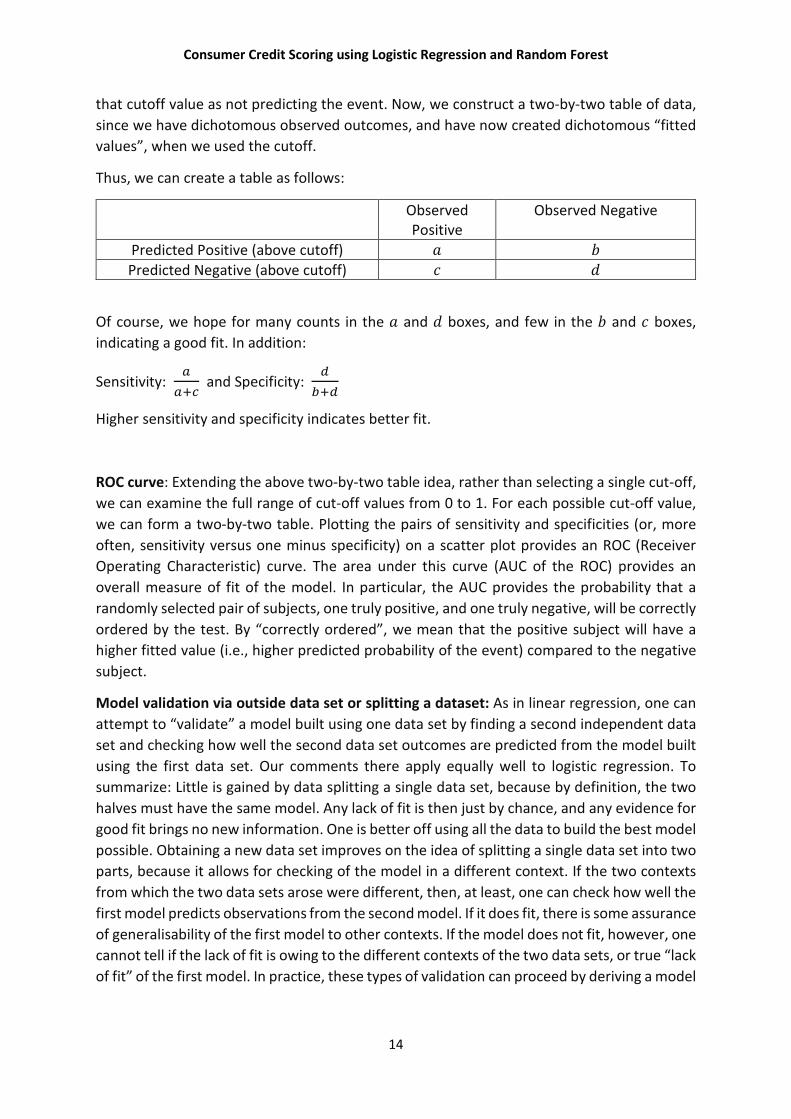
that cutoff value as not predicting the event. Now, we construct a two-by-two table of data,

since we have dichotomous observed outcomes, and have now created dichotomous “fitted

values”, when we used the cutoff.

Thus, we can create a table as follows:

Observed Positive

Observed Negative

Predicted Positive (above cutoff) � �

Predicted Negative (above cutoff) � �

Of course, we hope for many counts in the � and � boxes, and few in the � and � boxes,

indicating a good fit. In addition:

Sensitivity: �

�� and Specificity:

�

��

Higher sensitivity and specificity indicates better fit.

ROC curve: Extending the above two-by-two table idea, rather than selecting a single cut-off,

we can examine the full range of cut-off values from 0 to 1. For each possible cut-off value,

we can form a two-by-two table. Plotting the pairs of sensitivity and specificities (or, more

often, sensitivity versus one minus specificity) on a scatter plot provides an ROC (Receiver

Operating Characteristic) curve. The area under this curve (AUC of the ROC) provides an

overall measure of fit of the model. In particular, the AUC provides the probability that a

randomly selected pair of subjects, one truly positive, and one truly negative, will be correctly

ordered by the test. By “correctly ordered”, we mean that the positive subject will have a

higher fitted value (i.e., higher predicted probability of the event) compared to the negative

subject.

Model validation via outside data set or splitting a dataset: As in linear regression, one can

attempt to “validate” a model built using one data set by finding a second independent data

set and checking how well the second data set outcomes are predicted from the model built

using the first data set. Our comments there apply equally well to logistic regression. To

summarize: Little is gained by data splitting a single data set, because by definition, the two

halves must have the same model. Any lack of fit is then just by chance, and any evidence for

good fit brings no new information. One is better off using all the data to build the best model

possible. Obtaining a new data set improves on the idea of splitting a single data set into two

parts, because it allows for checking of the model in a different context. If the two contexts

from which the two data sets arose were different, then, at least, one can check how well the

first model predicts observations from the second model. If it does fit, there is some assurance

of generalisability of the first model to other contexts. If the model does not fit, however, one

cannot tell if the lack of fit is owing to the different contexts of the two data sets, or true “lack

of fit” of the first model. In practice, these types of validation can proceed by deriving a model


15

and estimating its coefficients in one data set, and then using this model to predict the Y

variable from the second data set. One can then check the residuals, and so on.

4.6 Stepwise Logistic Regression:

In stepwise logistic regression, variables are selected for inclusion or exclusion from the model

in a sequential fashion based solely on statistical criteria. The stepwise approach is useful and

intuitively appealing in that it builds models in a sequential fashion and it allows for the

examination of a collection of models which might not otherwise have been examined. The

two main versions of the stepwise procedure are forward selection followed by a test for

backward elimination or backward elimination followed by forward selection. Forward

selection starts with no variables and selects variables that best explains the residual (the

error term or variation that has not yet been explained.) Backward elimination starts with all

the variables and removes variables that provide little value in explaining the response

function. Stepwise method are combinations that have the same starting point by consider

inclusion and elimination of variables at each iteration.

Any stepwise procedure for selection or deletion of variables from a model is

based on a statistical algorithm that checks for the "importance" of variables and either

includes or excludes them on the basis of a fixed decision rule. The "importance" of a variable

is defined in terms of a measure of statistical significance of the coefficient for the variable.

The statistic used depends on the assumptions of the model. In stepwise linear regression an

F-test is used since the errors are assumed to be normally distributed. In logistic regression

the errors are assumed to follow a binomial distribution, and the significance of the variable

is assessed via the likelihood ratio chi-square test. At any step in the procedure the most

important variable, in statistical terms, is the one that produces the greatest change in the

log-likelihood relative to a model not containing the variable.

4.7 K-fold cross validation:

This approach involves randomly dividing the set of observation into � groups, or folds, of

approximately equal size. The first fold is treated as a validation set, and the method is fit on

the remaining � − 1 folds. The mean squared error �� then computed on the observations

in the held out fold. This procedure is repeated � times. This process results in � estimates

of the test error. The � − fold CV is computed by averaging these values.

��(�) =1

��

�

��


16

Chapter 5: Random Forest

5.1 An Overview of classification:

The linear regression model assumes that the response variable � is quantitative. But in many

situations, the response variable is instead qualitative. For example, eye colour is qualitative,

taking on values blue, brown, or green. Often qualitative variables are referred to as

categorical; we will use these terms interchangeably. In this chapter, we study approaches for

predicting qualitative responses, a process that is known as classification. Predicting a

qualitative response for an observation can be referred to as classifying that observation,

since it involves assigning the observation to a category, or class. On the other hand, often

the methods used for classification first predict the probability of each of the categories of a

qualitative variable, as the basis for making the classification. In this sense they also behave

like regression methods.

Models of data with a categorical response are called classifiers. A classifier is

built from training data, for which classifications are known. The classifier assigns new test

data to one of the categorical levels of the response. Previously we have discussed one of the

most widely used classifier: Logistic regression.

5.2 Introduction to random forest:

To take advantage of the sheer size of modern data sets, we now need learning algorithms

that scale with the volume of information, while maintaining sufficient statistical efficiency.

Random forests, devised by Breiman in the early 2000s (Breiman 2001), are part of the list of

the most successful methods currently available to handle data in these cases. This supervised

learning procedure, influenced by the early work of Amit and Geman (1997), Ho (1998), and

Dietterich (2000), operates according to the simple but effective “divide and conquer”

principle: sample fractions of the data, grow a randomized tree predictor on each small piece,

then paste (aggregate) these predictors together.

What has greatly contributed to the popularity of forests is the fact that they can be

applied to a wide range of prediction problems and have few parameters to tune. Aside from

being simple to use, the method is generally recognized for its accuracy and its ability to deal

with small sample sizes and high-dimensional feature spaces. At the same time, it is easily

parallelizable and has, therefore, the potential to deal with large real-life systems. Howard

(Kaggle) and Bowles (Biomatica) claim in Howard and Bowles (2012) that ensembles of

decision trees—often known as “random forests”—have been the most successful general-

purpose algorithm in modern times, while Varian, Chief Economist at Google, advocates in

Varian (2014) the use of random forests in econometrics.

The difficulty in properly analysing random forests can be explained by the black-

box flavor of the method, which is indeed a subtle combination of different components.

Among the forests’ essential ingredients, both bagging (Breiman 1996) and the Classification

And Regression Trees (CART)-split criterion (Breiman et al. 1984) play critical roles. Bagging (a

contraction of bootstrap-aggregating) is a general aggregation scheme, which generates


17

bootstrap samples from the original data set, constructs a predictor from each sample, and

decides by averaging. It is one of the most effective computationally intensive procedures to

improve on unstable estimates, especially for large, high-dimensional data sets, where finding

a good model in one step is impossible because of the complexity and scale of the problem

(Bühlmann and Yu 2002; Kleiner et al. 2014; Wager et al. 2014) However, while bagging and

the CART-splitting scheme play key roles in the random forest mechanism, both are difficult

to analyse with rigorous mathematics, thereby explaining why theoretical studies have so far

considered simplified versions of the original procedure. This is often done by simply ignoring

the bagging step and/or replacing the CART-split selection by a more elementary cut protocol.

As well as this, in Breiman’s (2001) forests, each leaf (that is, a terminal node) of individual

trees contains a small number of observations, typically between 1 and 5.

5.3 Definition of random forests:

A random forest is a classifier consisting a collection of tree-structured classifiers

{ℎ(�,Θ�),� = 1,… … … } where {Θ�} are independent and identically distributed

random vectors and each tree casts a unit vote for the most popular class at input �.

5.4 Basic principles:

Let us start with a word of caution. The term “random forests” is a bit ambiguous. For some

authors, it is but a generic expression for aggregating random decision trees, no matter how

the trees are obtained. For others, it refers to Breiman’s (2001) original algorithm. We

essentially adopt the second point of view in the present survey.

Our objective in this section is to provide a concise but mathematically precise

presentation of the algorithm for building a random forest. The general framework is

nonparametric regression estimation, in which an input random vector � ∈ � ⊂ ℝ� is

observed, and the goal is to predict the square integrable random response � ∈ ℝ by

estimating the regression

function �(�) = �[�|� = �]. With this aim in mind we assume that we have training sample

�� = �(��,��),… … … .,(��,��)� of independent random variables distributed as the

independent prototype pair (�,�).The goal is to use the dataset �� to construct an estimate

��:� → ℝ of the function �. In this respect we say that regression function estimate �� is

(mean squared error) is consistent if �[��(�) − �(�)]� → 0 as � → ∞ (the expectation is

evaluated over � and the sample ��.

A random forest is a predictor consisting of a collection of � randomized

regression trees. For the �� tree is the family, the predicted value at the query point � is

denoted by ��; Θ�,��, where Θ�,… … … ..,Θ� are independent random variables

distributed same as the generic random variable Θ and independent of ��. In practice, the

variable Θ is used to resample the training set prior to the growing of individual trees and to

select the successive directions for splitting. In mathematical terms the �� tree estimate takes

the form:


18

��; Θ�,�� = ��∈��;��,��

��; Θ�,��∈��

∗ ��

Where ��∗ �Θ�� is the set of data points selected prior to tree construction,

��; Θ�,�� is the cell containing � and ��; Θ�,�� is the number of (pre-selected)

points that fall into ��; Θ�,��.

At this stage we note that the trees are combined to form the (finite) forest

estimate

��(�; Θ�,… … … ..,Θ�,��) =�

�∑ ��; Θ�,��

�� . (1)

In the R package randomForest , the default value of �(the number of trees in

the forest) is ntree=500. Since � may be chosen arbitrarily large (limited only by available

computing resources), it makes sense, from the modelling point of view to let � tend to

infinity, and consider instead of (1) the (infinite) forest estimate

��,�(�; ��) = ��; Θ�,��.

In this definition, �� denotes the expectation with respect to the random

parameter �, conditional on ��. In fact, the operation "� → ∞" is justified by the law of large

numbers which asserts that almost surely, conditional on ��:

lim�→ �

��,�(�; Θ1,… … … ..,Θ�,��) = ��,�(�; ��).


19

Chapter 6: An overview of LASSO:

6.1 Introduction

The “lasso” minimizes the residual sum of squares subject to the sum of absolute value of the

coefficients being less than a constant. Because of the nature of this constant it tends to

produce some coefficients that are exactly 0 and hence give interpretable models.

The two standard techniques for improving the OLS estimates, subset selection

and ridge regression, both have drawbacks. Subset selection provides interpretable models

but can be extremely variable because it is a discrete process- regressors are either retained

or dropped from the model. Small changes in the data set can result in very different models

being selected and this can reduce prediction accuracy. Ridge regression is a continuous

process that shrinks coefficients and hence is more stable: however, it does not set any

coefficients to 0 and hence does not give an easily interpretable model.

The lasso shrinks some coefficients and sets others to zero and hence tries to

retain good features of both subset selection and ridge regression.

6.2 Definition

Suppose that we have the data (��,��),� = 1,2,… … … ,�, where �� = ��,��,… … … ,��

are the predictor variables and �� are the responses. As in the regression set-up, we assume

that either the observations are independent or that the �� are conditionally independent

given the ��. We assume that �� are standardized so that ∑ �� ⁄ = 0� and ∑ �� = 1.⁄�

Letting �� = ��,… … ,��

��

, the lasso estimate ��,�� is defined by

��,�� = argmin �∑ �y� − α − ∑ ��

�� subject to ∑ |�� | ≤ �.

Here � ≥ 0 is a tuning parameter. Now for all �, the solution for � is �� = ��. We can assume

without loss of generality that �� = 0 and hence omit �.

We can also write the lasso problem in the equivalent Lagrangian form.

� �yi− α − � ��

�

��

��

��

+ � � |��|

�

��

= �� + � � |��|

�

��

Here we say that lasso generates sparse models, i.e. models that involves only a subset of

variables.


20

Chapter 7: Analysis of German credit data:

Here I first perform parametric classification e.g. Logistic regression, shall see how the model fits,

infer about it then I will use non-parametric classification e.g. Random Forest.

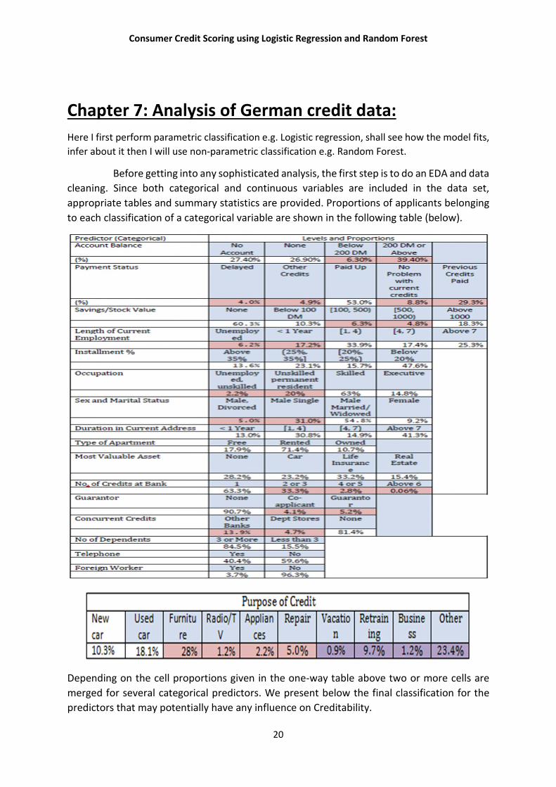
Before getting into any sophisticated analysis, the first step is to do an EDA and data

cleaning. Since both categorical and continuous variables are included in the data set,

appropriate tables and summary statistics are provided. Proportions of applicants belonging

to each classification of a categorical variable are shown in the following table (below).

Depending on the cell proportions given in the one-way table above two or more cells are

merged for several categorical predictors. We present below the final classification for the

predictors that may potentially have any influence on Creditability.


21

Account Balance: No account (1), None (No balance) (2), Some Balance (3)

Payment Status: Some Problems (1), Paid Up (2), No Problems (in this bank) (3)

Savings/

Stock Value: None, Below 100 DM, [100, 1000] DM, Above 1000 DM

Employment Length: Below 1 year (including unemployed), [1, 4), [4, 7), Above 7

Sex/Marital Status: Male Divorced/Single, Male Married/Widowed, Female

No of Credits at this bank: 1, More than 1

Guarantor: None, Yes

Concurrent Credits: Other Banks or Dept. Stores, None

Foreign Worker variable may be dropped from the study

Purpose of Credit: New car, Used car, Home Related, Other

Cross-tabulation of the some of the 9 predictors as defined above with Creditability is shown

below. The proportions shown in the cells are column proportions and so are the marginal

proportions. For example, 30% of 1000 applicants have no account and another 30% have no

balance while 40% have some balance in their account. Among those who have no account

135 are found to be Creditable and 139 are found to be Non-Creditable. In the group with no

balance in their account, 40% were found to be on-Creditable whereas in the group having

some balance only 1% are found to be Non-Creditable.

| Acc.Balance Creditability | 1 | 2 | 3 | Row Total | --------------|-----------|-----------|-----------|-----------| 0 | 240 | 14 | 46 | 300 | | 0.4 | 0.2 | 0.1 | | --------------|-----------|-----------|-----------|-----------| 1 | 303 | 49 | 348 | 700 | | 0.6 | 0.8 | 0.9 | | --------------|-----------|-----------|-----------|-----------| Column Total | 543 | 63 | 394 | 1000 | | 0.5 | 0.1 | 0.4 | | --------------|-----------|-----------|-----------|-----------|

| Payment. Status Creditability | 1 | 2 | 3 | Row Total | --------------|-----------|-----------|-----------|-----------| 0 | 53 | 169 | 78 | 300 | | 0.6 | 0.3 | 0.2 | | --------------|-----------|-----------|-----------|-----------| 1 | 36 | 361 | 303 | 700 | | 0.4 | 0.7 | 0.8 | | --------------|-----------|-----------|-----------|-----------| Column Total | 89 | 530 | 381 | 1000 | | 0.1 | 0.5 | 0.4 | | --------------|-----------|-----------|-----------|-----------| | Savings Creditability | 1 | 2 | 3 | Row Total | --------------|-----------|-----------|-----------|-----------| 0 | 217 | 34 | 49 | 300 | | 0.4 | 0.3 | 0.2 | | --------------|-----------|-----------|-----------|-----------| 1 | 386 | 69 | 245 | 700 |


22

| 0.6 | 0.7 | 0.8 | | --------------|-----------|-----------|-----------|-----------| Column Total | 603 | 103 | 294 | 1000 | | 0.6 | 0.1 | 0.3 | | --------------|-----------|-----------|-----------|-----------| | Employment. Length Creditability | 1 | 2 | 3 | Row Total | --------------|-----------|-----------|-----------|-----------| 0 | 197 | 39 | 64 | 300 | | 0.3 | 0.2 | 0.3 | | --------------|-----------|-----------|-----------|-----------| 1 | 376 | 135 | 189 | 700 | | 0.7 | 0.8 | 0.7 | | --------------|-----------|-----------|-----------|-----------| Column Total | 573 | 174 | 253 | 1000 | | 0.6 | 0.2 | 0.3 | | --------------|-----------|-----------|-----------|-----------| | No_of_Credits Creditability | 1 | 2 | Row Total | --------------|-----------|-----------|-----------| 0 | 200 | 100 | 300 | | 0.3 | 0.3 | | --------------|-----------|-----------|-----------| 1 | 433 | 267 | 700 | | 0.7 | 0.7 | | --------------|-----------|-----------|-----------| Column Total | 633 | 367 | 1000 | | 0.6 | 0.4 | | --------------|-----------|-----------|-----------| Summary statistics for continuous variables:

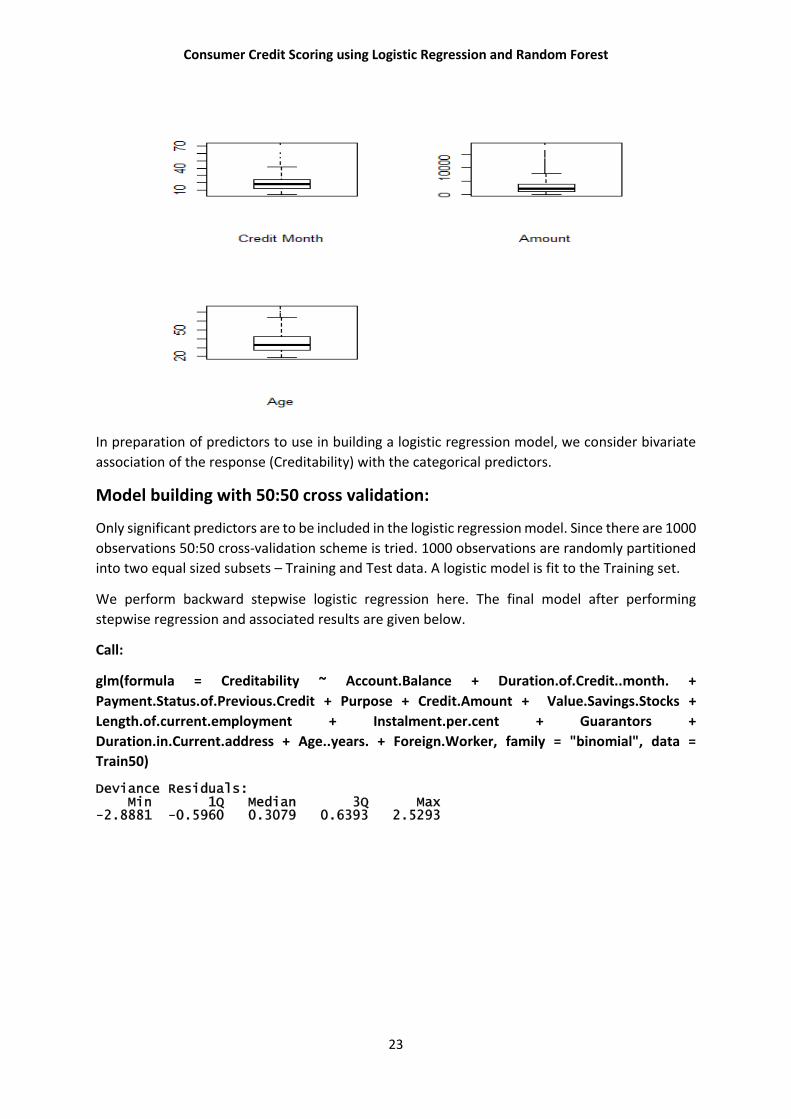
All the three continuous variables show marked positive skewness. Boxplots bear this out even more clearly.


23

In preparation of predictors to use in building a logistic regression model, we consider bivariate

association of the response (Creditability) with the categorical predictors.

Model building with 50:50 cross validation:

Only significant predictors are to be included in the logistic regression model. Since there are 1000

observations 50:50 cross-validation scheme is tried. 1000 observations are randomly partitioned

into two equal sized subsets – Training and Test data. A logistic model is fit to the Training set.

We perform backward stepwise logistic regression here. The final model after performing

stepwise regression and associated results are given below.

Call:

glm(formula = Creditability ~ Account.Balance + Duration.of.Credit..month. +

Payment.Status.of.Previous.Credit + Purpose + Credit.Amount + Value.Savings.Stocks +

Length.of.current.employment + Instalment.per.cent + Guarantors +

Duration.in.Current.address + Age..years. + Foreign.Worker, family = "binomial", data =

Train50)

Deviance Residuals: Min 1Q Median 3Q Max -2.8881 -0.5960 0.3079 0.6393 2.5293


24

Null deviance: 610.86 on 499 degrees of freedom Residual deviance: 408.48 on 463 degrees of freedom AIC: 482.48

If we want to see which variables are dropped, we can see here:

Step df Deviance Residual.df Residual.Dev AIC

1 NA NA 445 391.3381 501.3381

2 Most. Valuable. available.asset

3 0.8845622 448 392.2226 496.2226

3 Occupation

3 1.2792911 451 393.5019 491.5019

4 No.of.Credits.at.this.Bank

3 2.3052671 454 395.8072 487.8072

5 No.of. dependents

1 0.3380494 455 396.1452 486.1452

6 Concurrent.Credits

2 2.7130649 457 395.8583 484.8583

7 Type.of.apartment

2 2.5642810 459 401.4226 483.4226


25

Step df Deviance Residual.df Residual.Dev AIC

8 Telephone

1 1.4482482 460 402.8078 482.8078

9 Sex...Marital.Status

3 5.6066694 463 408.4775 482.8075

Goodness of fit test:

Chi-square goodness of fit: Here test statistic �� = 483.2076

And � − �� =0.9674946. A large � − �� indicating the lack of fit.

Hosmer-Lemshow Test:

$C

Hosmer-Lemeshow C statistic

data: fit50 and TrainRspns

X-squared = 7.1672, df = 8, p-value = 0.5187

$H

Hosmer-Lemeshow H statistic

data: fit50 and TrainRspns

X-squared = 7.3264, df = 8, p-value = 0.5019

Now I do a classification table to check how accurate the model predicts with different cutoff values

of probability.

Test Data 50% Threshold 40% Threshold 75% Threshold

Creditable Non-creditable



Creditable 350 296 54 311 39 247 103

Non-creditable

150 80 70 94 56 50 100

Total 500 Accuracy= (70+296)/500 =73.2%

Accuracy= (311+56)/500 =73.4%

Accuracy= (247+100)/500 =69.4%

From these I can conclude that cutoff probability 0.4 gives better accuracy in predicting than others .

Now let us have a looks how the model performs for different samples of the original data . Here I

am going to use k-fold cross validation. The most common variation of cross validation is 10-fold

cross-validation.

Generalized Linear Model 1000 samples 20 predictor 2 classes: '0', '1' No pre-processing


26

Resampling: Cross-Validated (10 fold, repeated 10 times) Summary of sample sizes: 900, 900, 900, 900, 900, 900, ... Resampling results: Accuracy Kappa 0.7478 0.3642265

Now let’s see if there is any improvement in accuracy via confusion matrix.

Confusion Matrix and Statistics Reference Prediction 0 1 0 74 37 1 76 313 Accuracy : 0.774 95% CI : (0.7348, 0.8099) No Information Rate : 0.7 P-Value [Acc > NIR] : 0.0001305 Kappa : 0.4187 Mcnemar's Test P-Value : 0.0003506 Sensitivity : 0.4933 Specificity : 0.8943 Pos Pred Value : 0.6667 Neg Pred Value : 0.8046 Prevalence : 0.3000 Detection Rate : 0.1480 Detection Prevalence : 0.2220 Balanced Accuracy : 0.6938 'Positive' Class : 0

Here we can see in comparison to previous classification table we have a slight improvement in accuracy, here we have 77.4% accuracy in predicting the true values of �. Now the question remains, is this model is a good fit? What are the effects of covariates

in misclassification? How does it affect the model? I discuss these later. First let’s see how the

nonparametric classifier e.g. Random forest performs.

Random forests are very good in that it is an ensemble learning method used for classification

and regression. It uses multiple models for better performance that just using a single tree

model. In addition, because many sample are selected in the process a measure of variable

importance can be obtain and this approach can be used for model selection and can be

particularly useful when forward/backward stepwise selection is not appropriate and when

working with an extremely high number of candidate variables that need to be reduced.

Here I do an unsupervised random forest method. Which leads to the following

results:

Call: randomForest(formula = as.factor(Creditability) ~ ., data = Train50, ntree = 400, importance = TRUE, proximity = TRUE) Type of random forest: classification Number of trees: 400 No. of variables tried at each split: 4 OOB estimate of error rate: 24% Confusion matrix: 0 1 class.error


27

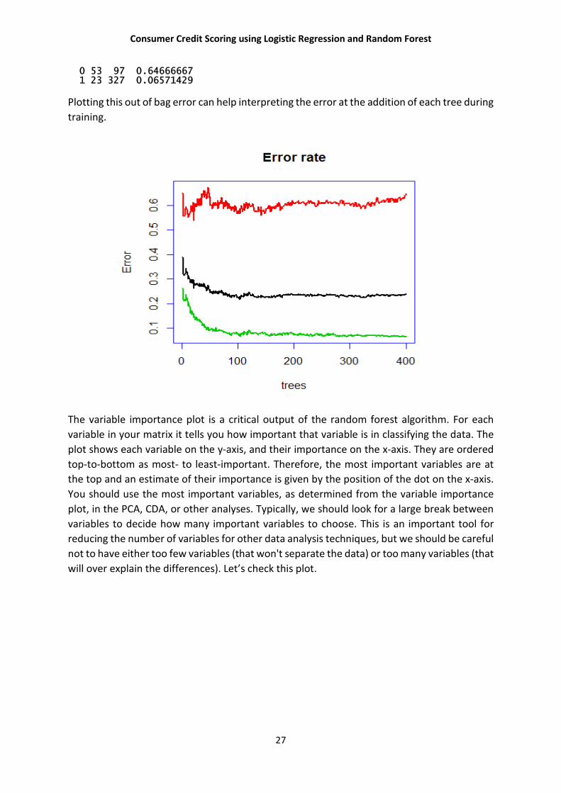
0 53 97 0.64666667 1 23 327 0.06571429

Plotting this out of bag error can help interpreting the error at the addition of each tree during

training.

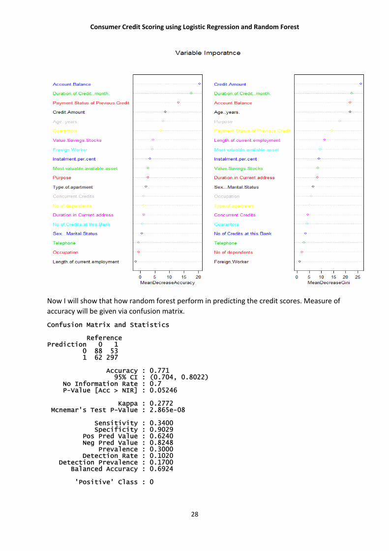
The variable importance plot is a critical output of the random forest algorithm. For each

variable in your matrix it tells you how important that variable is in classifying the data. The

plot shows each variable on the y-axis, and their importance on the x-axis. They are ordered

top-to-bottom as most- to least-important. Therefore, the most important variables are at

the top and an estimate of their importance is given by the position of the dot on the x-axis.

You should use the most important variables, as determined from the variable importance

plot, in the PCA, CDA, or other analyses. Typically, we should look for a large break between

variables to decide how many important variables to choose. This is an important tool for

reducing the number of variables for other data analysis techniques, but we should be careful

not to have either too few variables (that won't separate the data) or too many variables (that

will over explain the differences). Let’s check this plot.


28

Now I will show that how random forest perform in predicting the credit scores. Measure of

accuracy will be given via confusion matrix.

Confusion Matrix and Statistics Reference Prediction 0 1 0 88 53 1 62 297 Accuracy : 0.771 95% CI : (0.704, 0.8022) No Information Rate : 0.7 P-Value [Acc > NIR] : 0.05246 Kappa : 0.2772 Mcnemar's Test P-Value : 2.865e-08 Sensitivity : 0.3400 Specificity : 0.9029 Pos Pred Value : 0.6240 Neg Pred Value : 0.8248 Prevalence : 0.3000 Detection Rate : 0.1020 Detection Prevalence : 0.1700 Balanced Accuracy : 0.6924 'Positive' Class : 0


29

So form above we have found that the accuracy in prediction is 77.1%. Which is quite an

improvement from the logistic regression procedure we performed before.

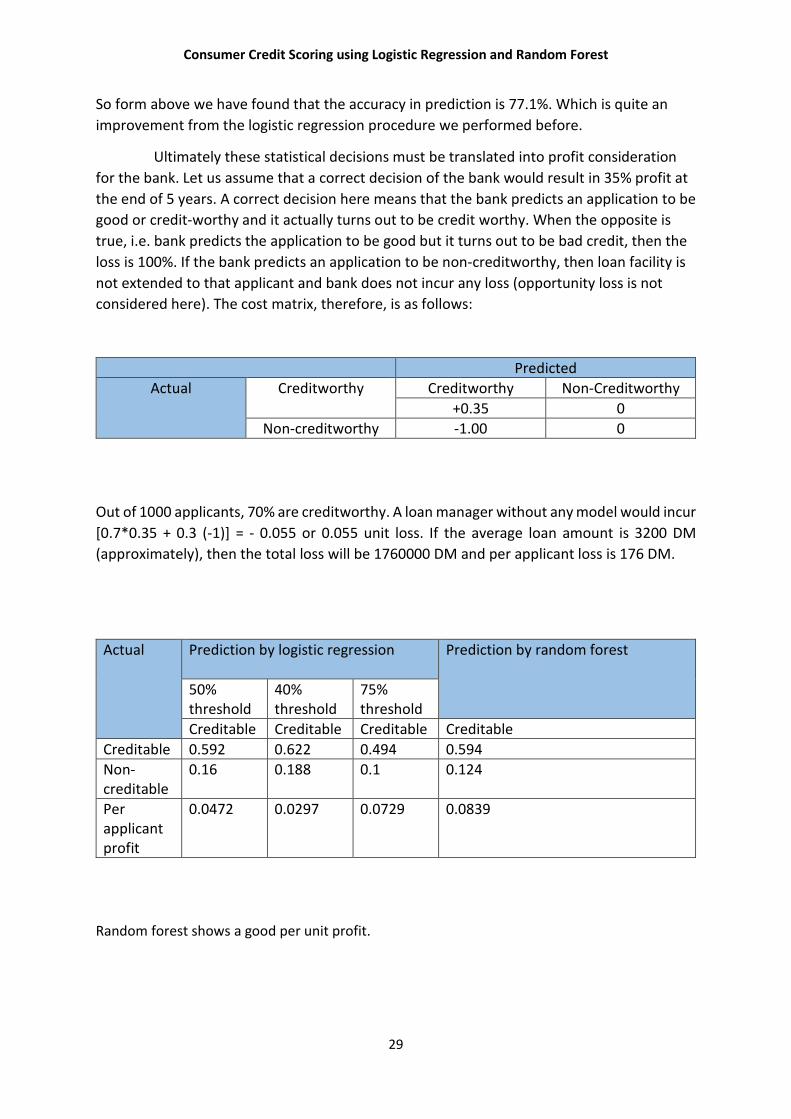
Ultimately these statistical decisions must be translated into profit consideration

for the bank. Let us assume that a correct decision of the bank would result in 35% profit at

the end of 5 years. A correct decision here means that the bank predicts an application to be

good or credit-worthy and it actually turns out to be credit worthy. When the opposite is

true, i.e. bank predicts the application to be good but it turns out to be bad credit, then the

loss is 100%. If the bank predicts an application to be non-creditworthy, then loan facility is

not extended to that applicant and bank does not incur any loss (opportunity loss is not

considered here). The cost matrix, therefore, is as follows:

Predicted

Actual Creditworthy Creditworthy Non-Creditworthy

+0.35 0

Non-creditworthy -1.00 0

Out of 1000 applicants, 70% are creditworthy. A loan manager without any model would incur

[0.7*0.35 + 0.3 (-1)] = - 0.055 or 0.055 unit loss. If the average loan amount is 3200 DM

(approximately), then the total loss will be 1760000 DM and per applicant loss is 176 DM.

Actual Prediction by logistic regression Prediction by random forest

50% threshold

40% threshold

75% threshold

Creditable Creditable Creditable Creditable

Creditable 0.592 0.622 0.494 0.594

Non-creditable

0.16 0.188 0.1 0.124

Per applicant profit

0.0472 0.0297 0.0729 0.0839

Random forest shows a good per unit profit.


30

Limitations: Though we have performed logistic regression and random forest and get an

accuracy of predicting 73.4 and 77.1 respectively (not considering the k-fold cross validation

case). But did it actually perform that well?

If we plot a scatterplot for the data, we can see lots of correlations among the variables.

In r we perform a scatterplot matrix and see too much correlations among the variables. Plot

is given below.

From the plot we can see that there is lots of correlations among the 12 covariates which we

found after performing logistic regression. So there exists multicollinearity. One way to

improve from this is to perform a variable reduction technique, e.g. Principal component

analysis. After performing principal component analysis it can be seen that, the first principal

component explains 95% of the variation which is the proof of existence of multicollinearity.

Now as we have 12 covariates in the improved model but it is really difficult to check the

effects of all these covariates in the misclassification. So we look into the absolute value of

t-statistic of each model parameter to assess the relative importance of each individual

predictor of the model. Now selecting only three most important predictors and vary them

according to their levels and fix remaining nine predictors to their mean effect. Then we try

to plot the true positive prediction probability i.e. �(� = �)� and false positive prediction

probability i.e �(� ≠ ��) against the samples. The result comes out as:


31

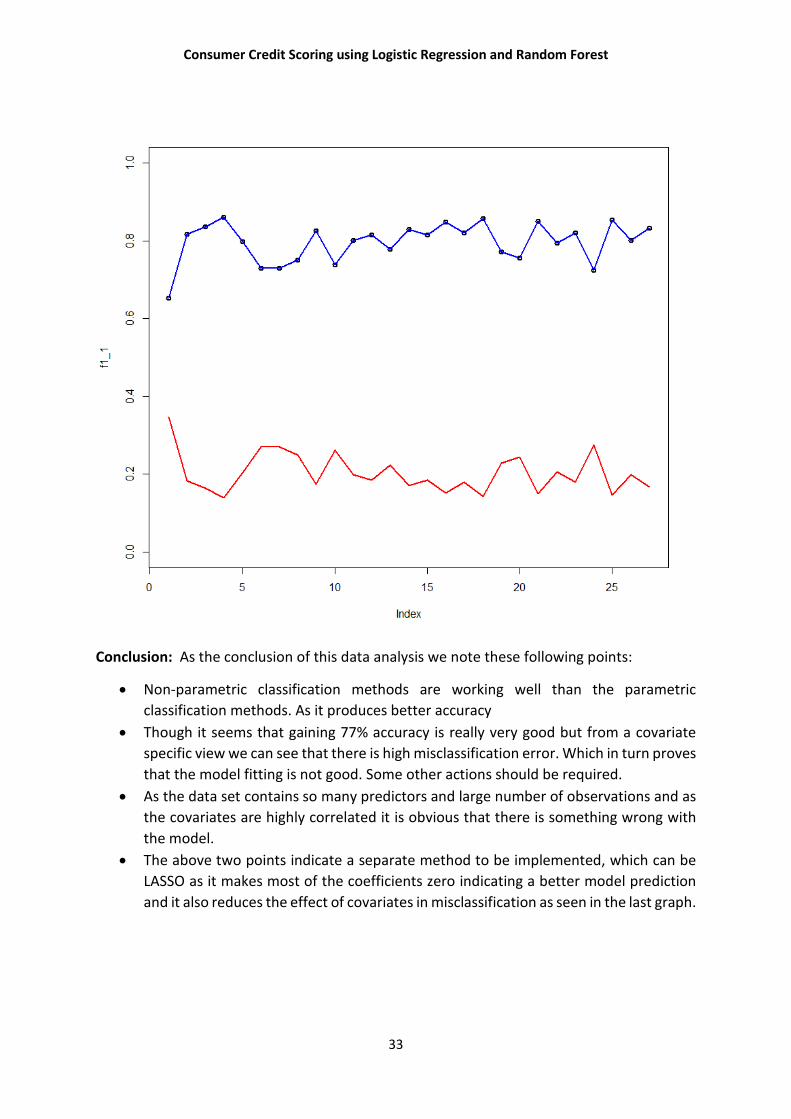
As we can see from the above plot the blue line represent true positive prediction

probability and the red line represent false positive prediction probability. As both the red

line cuts the blue line in many points which should be higher than the red line, we can

conclude that the misclassification error is highly affected by the covariate.

Now as the first PC explains most of the variation, I use the first pc to model the data

then plot the graph in the above mentioned way to see is there any improvement.

We can see from the graph that there is slight improvement as the blue line is a bit higher

though still there is a cut between red and blue line.

Then what should be the procedure to improve this fact? The answer is LASSO.


32

When we perform LASSO we can see that out of 12 coefficients in the final model 5

coefficients are exactly 0. When we plot the training MSE as a function we have the plot:

From here we can find the value of � which minimizes the training MSE, i.e. �=0.0004821952.

Now if we want to see the effects of covariates in the misclassification we can see that by the

plot that true positive prediction probability(blue line) is significantly higher than the false

positive prediction probability(red line). So now we can say that by LASSO we have

interpreted a good model.


33

Conclusion: As the conclusion of this data analysis we note these following points:

Non-parametric classification methods are working well than the parametric

classification methods. As it produces better accuracy

Though it seems that gaining 77% accuracy is really very good but from a covariate

specific view we can see that there is high misclassification error. Which in turn proves

that the model fitting is not good. Some other actions should be required.

As the data set contains so many predictors and large number of observations and as

the covariates are highly correlated it is obvious that there is something wrong with

the model.

The above two points indicate a separate method to be implemented, which can be

LASSO as it makes most of the coefficients zero indicating a better model prediction

and it also reduces the effect of covariates in misclassification as seen in the last graph.


34

Appendix:

Appendix 1:

R codes:

# loading the data set

DATA<-read.csv("C:/Users/Hirak/Desktop/german_credit.csv",header=TRUE)

View(DATA)

names(DATA)

attach(DATA)

#Performing EDA

margin.table(prop.table(table(Duration.in.Current.address,Most.valuable.available.asset,Concurrent

.Credits,No.of.Credits.at.this.Bank,Occupation,No.of.dependents,Telephone,Foreign.Worker)),1)

margin.table(prop.table(table(Duration.in.Current.address,Most.valuable.available.asset,

Concurrent.Credits,No.of.Credits.at.this.Bank,Occupation,No.of.dependents,Telephone,

Foreign.Worker)),2)



Foreign.Worker)),3)



Foreign.Worker)),4)



Foreign.Worker)),5)



Foreign.Worker)),6)



Foreign.Worker)),7)



Foreign.Worker)),8)

#cross tables

library(gmodels)

CrossTable(Creditability,Acc.Balance,digits=1,prop.r=F,prop.t=F, prop.chisq=F, chisq=F)


35

CrossTable(Creditability,Payment.status, digits=1,prop.r=F, prop.t=F, prop.chisq=F, chisq=F)

CrossTable(Creditability,Savings,digits=1,prop.r=F,prop.t=F, prop.chisq=F, chisq=F)

CrossTable(Creditability,Employment.length,digits=1,prop.r=F, prop.t=F, prop.chisq=F, chisq=F)

CrossTable(Creditability,Sex_marital_status,digits=1,prop.r=F, prop.t=F, prop.chisq=F, chisq=F)

CrossTable(Creditability,No_of_Credits,digits=1,prop.r=F, prop.t=F, prop.chisq=F, chisq=F)

CrossTable(Creditability,Guarantor,digits=1,prop.r=F, prop.t=F, prop.chisq=F, chisq=F)

CrossTable(Creditability,Concurrent_credit,digits=1,prop.r=F, prop.t=F, prop.chisq=F, chisq=F)

CrossTable(Creditability,Purpose_of_credit,digits=1,prop.r=F,prop.t=F, prop.chisq=F, chisq=F)

CrossTable(Creditability,Type.of.apartment,digits=1,prop.r=F,prop.t=F, prop.chisq=F, chisq=F)

CrossTable(Creditability,No.of.dependents,digits=1,prop.r=F,prop.t=F, prop.chisq=F, chisq=F)

CrossTable(Creditability,Instalment.per.cent,digits=1,prop.r=F,prop.t=F, prop.chisq=F, chisq=F)

#Summary statistics for continuous variables

summary(Duration.of.Credit..month.);sd(Duration.of.Credit..month.)

summary(Credit.Amount);sd(Credit.Amount)

summary(Age..years.);sd(Age..years.)

#boxplot for cont. variables

par(mfrow=c(2,2))

boxplot(Duration.of.Credit..month., bty="n",xlab = "Credit Month", cex=0.4) # For boxplot

boxplot(Credit.Amount, bty="n",xlab = "Amount", cex=0.4)

boxplot(Age..years., bty="n",xlab = "Age", cex=0.4)

# Logistic model

for (i in c(2,4:5,7:13,15:20)){

DATA[,i] <- as.factor(DATA[,i])

}

nrow(DATA)

set.seed(50) # setting the random number seed for splitting the dataset

indexes = sample(1:nrow(DATA), size=0.5*nrow(DATA)) # Random sample of 50% of row numbers

created

Train50 <- DATA[indexes,]

Test50 <- DATA[-indexes,]

indVariables <- colnames(DATA[,2:21]);indVariables


36

# getting the independent variables, the last column is the dependent variable

rhsOfModel <- paste(indVariables,collapse="+")

# creating the right hand side of the model expression

rhsOfModel

model <- paste("Creditability ~ ",rhsOfModel)

# creating the text model

model

frml <- as.formula(model) # converting the above text into a formula

frml

library(MASS) # loading the library MASS for stepwise regression

TrainModel <- glm(formula=frml,family="binomial",data=Train50)

# building the model on training data with LOGIT link (family = binomial

finalModel <- step(object=TrainModel)

summary(finalModel)# stepwise regression

finalModel$coefficients[1:21]

sum(residuals(finalModel,type="pearson")^2)

deviance(finalModel)

1-pchisq(deviance(finalModel),df.residual(finalModel))

summary(object=finalModel)

finalModel$anova

finalModel$fitted.values

fit50 <- fitted.values(finalModel)

fit50

library(MKmisc) # loading the library MKmisc for Hosmer Lemeshow Goodness of fit

HLgof.test(fit=fit50,obs=TrainRspns)

library(pROC) # loading library pROC for ROC curve

TestPred <- predict(object=finalModel,newdata=Test50, type="response")

# predicting the testing data

TestPredRspns <- ifelse(test= TestPred < 0.75, yes= 0, no= 1)

#Random Forest

library(randomForest)


37

rf50<-randomForest(as.factor(Creditability)~.,data=Train50,

ntree=400,importance=TRUE,proximity=TRUE)

rf50<-randomForest(as.factor(Creditability)~.,data=Train50,

ntree=400,importance=TRUE,proximity=TRUE,control=ctrl)

print(rf50)

summary(rf50)

plot.new()

plot(proximity(rf50))

plot(rf50, main="Error rate", lwd=2,lty=7,fg="blue",)

plot( importance(rf50), lty=2, pch=16,col="red")

lines(importance(rf50),col="blue",lty=6,lwd=2)

Test50_rf_pred <- predict(rf50,Test50,type="class")

confusionMatrix(Test50_rf_pred, Test50$Creditability)

#limitations

DT<-

data.frame(Creditability,as.numeric(Duration.in.Current.address),as.numeric(Age..years.),as.numeric

(Guarantors),as.numeric(Savings),as.numeric(Length.of.current.employment),as.numeric(Duration.o

f.Credit..month.),as.numeric(Credit.Amount),as.numeric(Purpose),as.numeric(Instalment.per.cent),a

s.numeric(Payment.status),as.numeric(Foreign.Worker),as.numeric(Acc.Balance))

pc_DT<-prcomp(DT[,2:13])

summary(prcomp(DT[,2:13]))

library(GGally)

ggpairs(DT[,2:13],)

for(i in 1:3){

for( j in 1:3){

for(k in 1:3){

(Acc.Balance=i & Payment.status=j & Savings=k)}}}

plot(f1,lwd=3)

lines(f2,col="red",lwd=2)

plot(f2,add=TRUE)

lines(f1,col="blue",lwd=2)

plot.new()

plot(f1_1,lwd=5)


38

lines(f2_1,col="red",lwd=2)

lines(f1_1,col="blue",lwd=2)

#lasso

x <- as.matrix(Train50_DT[, 2:13])

y <- as.matrix(Train50_DT[, 1])

cv <- cv.glmnet(x, y,nfolds = 100)

plot(cv)

mdl <- glmnet(x, y,lambda = cv$lambda.1se)

mdl$beta

plot.glmnet(mdl)

bestlam=cv$lambda.min

plot(f1_1,ylim=c(0.0,1),lwd=2)

lines(f1_1,col="blue",lwd=2)

lines(f2_1,col="red",lwd=2)

Appendix:2

Data set link: http://www.statistik.lmu.de/service/datenarchiv/kredit/kredit_e.html

For the description of variables and more information please go to this link .


39

ACKNOWLEDGEMET

It is an opportunity with much pleasure to acknowledge all those person, from whom I

received considerable help through the course of my dissertation work.

First and foremost, I would like to offer my profound deepest gratitude and

record my sense of obligation to Dr. Sibnarayan Guria, Head of the department,

Department of Statistics. His cordiality, civility and amicableness provided an apt

platform for me to work. His superintendence, suggestion and discussion at every stage

have helped me immensely to carry out this work in a better way.

I am sure, there are no such thanking words to express my gratitude to Dr.

Sumanta Adhya, Assistant Professor, Department of Statistics, West Bengal State

University without whose heartiest cooperation, guidance, suggestion my dissertation

work, may not be successfully completed. I have been highly profited by lively discussions

on various aspects of Knowledge, Computation and Programming during my dissertation

work.

I am grateful and thankful to all my classmates for their cooperation and

continuous support in various aspects of the work.

Last but not the least; I am grateful to all those people, who have helped me

directly or indirectly in case of successful completion of dissertation work.


40

References

Anderson, R. (2007). The Credit Scoring Toolkit: Theory and Practice for Retail

Credit Risk Management and Decision Automation

Carling, K; Jacobson, T; Linde, J and Roszbach, K. (2002). Capital Charges under

Basel II: Corporate Credit Risk Modeling and the Macro Economy Sveriges

Riksbank Working Paper Series No. 142

Hosmer, D.W. and Lemeshow, S. (2000). Applied Logistic Regression Second

Edition

Breiman L ( 2001) Random forests. Mach Learn 45:5–32

Breiman L ( 2003a) Setting up, using, and understanding random forests V3.1.

https://www.stat.berkeley.edu/~breiman/Using_random_forests_V3.1.pdf

Robert.J.Tibshirani(1996). Regression Shrinkage and selection via the LASSO,JASA

B(1996),58,No.1,pp.267-288

consumer credit scoring using logistic regression and random forest

Data & Analytics