Consumer Surplus

©1999, 2006,2010, 2011 by Peter Berck

Money Measures

• How much would you be willing to pay (WTP) for a new ski area?

• How much does it cost?• Shouldn’t build unless total WTP is greater

than total cost.• Need WTP in $. Need a money measure.

Overview

• TWTP and CS• Relation of EV, CV and CS• EV and CV for a publicly provided good• Adding over consumers

– private good– public good\

• WTA and WTP

Demand Curves

• Demand: Amount that will be purchased as a function of price p.

• (Inverse) Demand: Price consumers will pay for next unit as function of number of units consumed, q.

• P(Q) is willingness to pay for next unit– Marginal willingness to pay

Demand Slopes Down

• willing to pay a lot more for the first pint of water (especially on a hot day in the desert) than for the pint after you have 40 gallons.

• wtp decreases as quantity increases

Total Willingness to Pay

• Total Willingness to pay is area under demand.– demand price P(Q) is amount willing to pay for

next unit– So total willing to pay for Q units is P(1) +

P(2) + ...+ P(Q)• lower riemann sum and an approximation• the area under the demand curve between 0 and Q

units, which is the integral of demand, is (total) willingness to pay

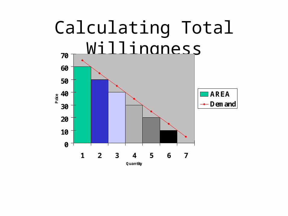
Calculating Total Willingness

0

10

20

30

40

50

60

70

1 2 3 4 5 6 7Quantity

Pri

ce AREADemand

Consumer Surplus

• Consumer surplus is willingness to pay less amount paid

• Amount paid is P Q

• Willingness is blue + green. Surplus is just the green

Consumer surplus is willingness to pay less amount paid

p

q

D

p

q

D

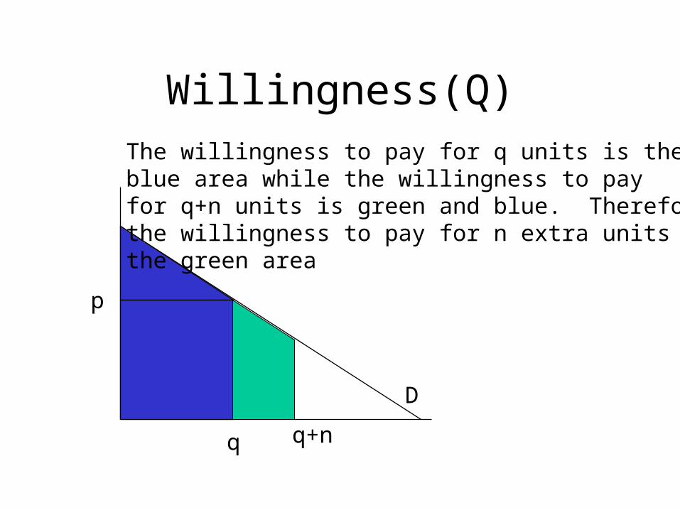
Willingness(Q)

q+n

The willingness to pay for q units is theblue area while the willingness to payfor q+n units is green and blue. Thereforethe willingness to pay for n extra units isthe green area

Money Measures-Theory

• Think of projects as lowering prices. – A new bridge lowers the price of crossing the

bay by making one wait less time in toll plaza lines

– A new ski area lowers price by making the commute from LA to skiing be shorter

Lots of things

• can be thought of as price changes– ipod mini brought price of carrying whole

music library around from essentially infinity to $200.

– new dam reduces price of electricity (because there is more of it and demand curves slope down.)

• taxes, like environmental taxes, are price increases.

p’

q’

D

Surplus and Price

q

Price increases from p to p’. CS wasgreen+yellow+ orange. After increase it is only green. CS changes by the wedgethat is yellow plus orange.

P

CS is an Approximate Measureand for markets goods a real

good approximationat that.

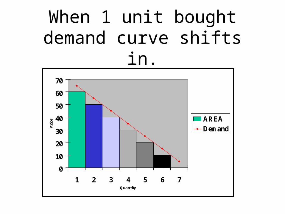
When 1 unit bought demand curve shifts in.

0

10

20

30

40

50

60

70

1 2 3 4 5 6 7Quantity

Pri

ce AREADemand

CS is easy

• All you got to do is calculate an area.• All you need is a demand curve• Trouble is that CS is an approximate money

measure• Lets look at some exact money measures

and see how compare

Exact money measures

• Equivalent Variation• Compensating Variation

– For a normal good, consumer surplus is in between these two measures. (Willig’s Theorem)

Equivalent Variation

• A consumer actually faces an increase in the price of a good from p0 to p1.

• That will make his utility go down from one indifference curve i to a lower indifference curve ii.

Thought Experiment: $ Equivalent

• If prices were left the same and instead money was taken away from the consumer– How much money would you need to take

away to reduce the consumers utility from i to ii?

– That amount of money is EV

EV Picture

Narrating the picture

• price doubled so now on new lower indifference curve ii.

• budget constraint III has original prices (parallel to budget constraint I) but is tangent to lower indiff curve ii.

• read change in income between I and III on the vertical axis (since the price of that good is 1).

EV

• The equivalent variation to a price change from p0 to p1 is the change in income that makes the consumer just as well off as if prices had changed from p0 to p1.

to remember EV..

• There are two equivalent ways to get the consumer to the new utility level:– change income– change prices

CV

• The compensating variation to a price change from p0 to p1 is the change in income that leaves the consumer just as well off at price p1 as he would have been with his original income at p0.

CV Picture

narrate cv

• Start out on indifference curve i. The price increases. Now you are on curve ii. How much money needed to get back?

• Budget constraint III has the new prices and enough income to get back to old indifference curve.

CV

• The change in income compensates for the change in price. The consumer is no better or worse off than before.

Willig shows that CS isn’t such a bad idea after all.

• for a price increase (for a normal good)– cv > CS > ev

• For the example in the textbook all three of these measures are within 63 cents and are on the order of $107.

• CS is more than good enough as a measure for a private good.

Does CS work for goods that are not bought?

• Candy bars are bought. They are private goods.

• The level of bio-diversity/wolves/air quality are all things that you cannot change by personally buying more. They are publicly provided goods.

Publicly Provided Goods

• If the government provides a good and– people have different preferences– then some people won’t get the amount they

like

• People who can buy (or sell) a good all have the price as their wtp for the next unit of the good.

• Not true if government gives the good.

• Wolves in the yellowstone ecosystem– some like em– some don’t– some like em more than others– everyone “gets” the same number—they are

just out there—get over it.

Diagram on next slide

• Has indifference curves. They are very sharply curved to create an extreme example.– You could draw some indifference curves not

quite so sharply curved and see if the general point still works

Exact money measure for wolves

• The “reality” is to get more wolves– Previous example was a higher price– Here it is a change in quantity

• More wolves increase utility• EV is the amount of added $ that increases

utility the same as the added wolves• CV is the amount of money removed to

return to original level of utility

EV and CV for Publicly Provided Good

0 5 10 15 20 25 30 350

5

10

15

20

25

30

35

Wolves

$

i ii

A B

C

EV and CV for Wolves

• Starting from point A, we calculate CV for 5 more wolves as follows. By adding 5 wolves, the consumer would be on indifference curve ii at point B. To return to indifference curve i, the consumer would need to give up $10 in income, so the CV is $10. For EV, the question is, how can we get the consumer back to indifference curve ii without providing wolves? The consumer can get from point A on i to point B on ii by adding 5 wolves, but even an infinite amount of income will not get her to ii, holding wolves constant; it will instead move her vertically along i. Hence EV is infinite.

Publicly provided conclusion

• If the indifference curves have are close to square shaped

• and the optimal amount (corners in this case) are not provided

• then ev and cv are very different.

Loose Ends

• So area under one person’s demand is twtp for that person.

• How do we find twtp for a private good for a market demand curve – Market demand = sum of individual demands

• Same question for many people and a public good.

Private good

• Market demand• For each price, add up the quantities each

consumer will buy. Horizontal addition of individual demand curves.

( ) ( )Total ii consumers

Q P Q P

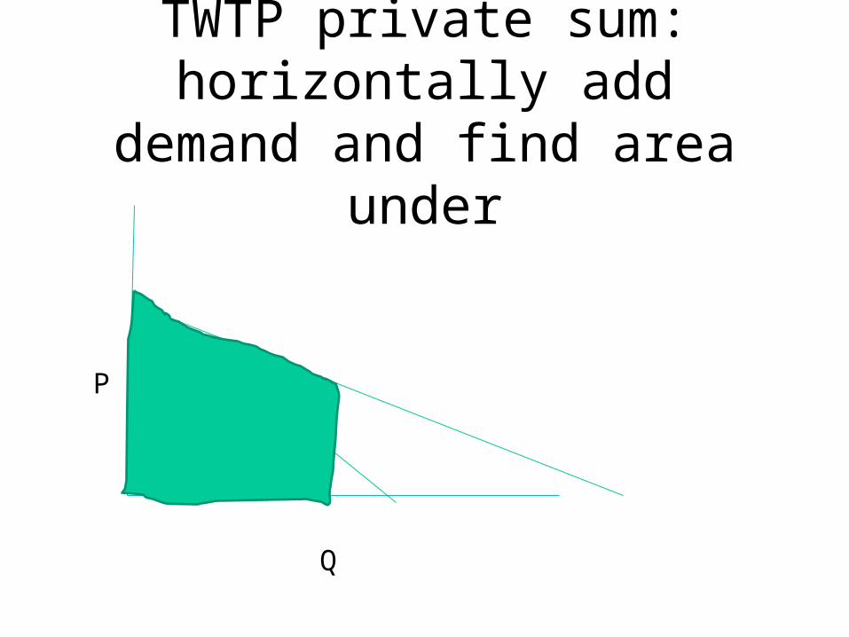
TWTP private sum: horizontally add demand and find area under

Q

P

Public Good

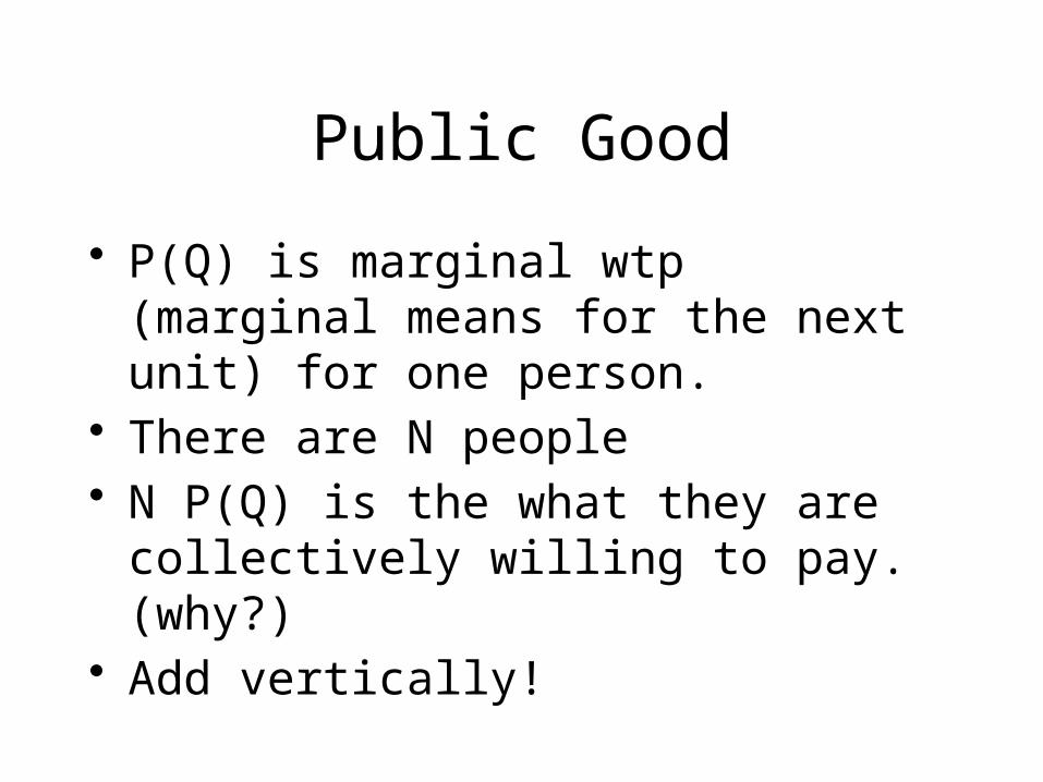
• P(Q) is marginal wtp (marginal means for the next unit) for one person.

• There are N people• N P(Q) is the what they are collectively

willing to pay. (why?)• Add vertically!

WTP for Public Good: vertically add and find area under

0 10 20 300

5

10

15

20

25

30

35

40

Wolves

$

Person 1's Demand

Person 2'sDemand

Total Demand

The marginal willingness to pay for a public good is the vertical sum of the individuals’ marginal willingness to pay values.

CS, EV, CV , WTP blind

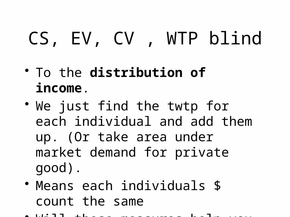
• To the distribution of income.• We just find the twtp for each individual

and add them up. (Or take area under market demand for private good).

• Means each individuals $ count the same• Will these measures help you explain why

Egypt subsidizes bread?

Valuation Questions

• How do CV and EV relate to questions you could ask people?– Willingness to pay– Willingness to accept

Remember!Utility Change is what

determines whether it is EV or CV

change only happens with EV!

WTP can lead to EV or CV

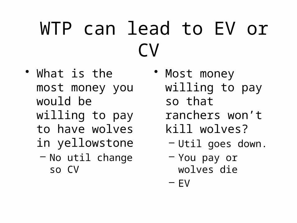
• What is the most money you would be willing to pay to have wolves in yellowstone– No util change so CV

• Most money willing to pay so that ranchers won’t kill wolves?– Util goes down.– You pay or wolves die– EV

WTA can lead to EV or CV

• Least money willing to accept instead of having increase in wolf numbers.– You get wolves or cash– Uitl changes– EV

• Least money willing to accept to allow ranchers to kill wolves.– Wolves die,– But you get paid– Uitl constant– CV

Using WTP to explain a two or more part tariff for Electricity

Price Discrimination

• Charging different consumers different prices.

• Could be the car salesman who tries to get all the twtp– Each consumer buys

one car

• Simplified electricity tariff– 10c/kwh for first

100kwh– Then 20c for all others– (inverted block)

• Diff prices for diff usage==diff prices for different people

Simplified Problem:

• Once $10b has been paid to construct a distribution system

• Electricity costs 10c/kwh to generate and distribute

• How to price?

If we charge 10c

• Then marginal willingness to pay will equal cost of producing next unit of power.

• Making more or less power won’t make any one better off without making someone else worse off

• Supply is horizontal and equals demand where we produce.

• But it won’t recover the 10b

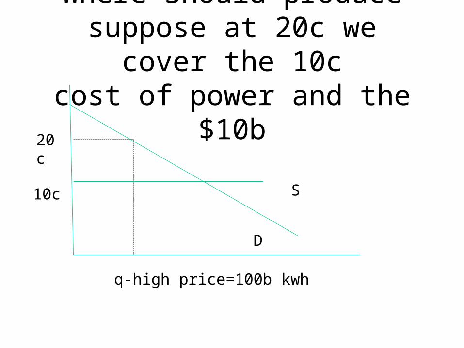
Where Should producesuppose at 20c we cover the 10c

cost of power and the $10b

S

D

10c

q-high price=100b kwh

20c

Can we do better with a two part tariff?

S

D

10c

q-high price

20c

q-10c price

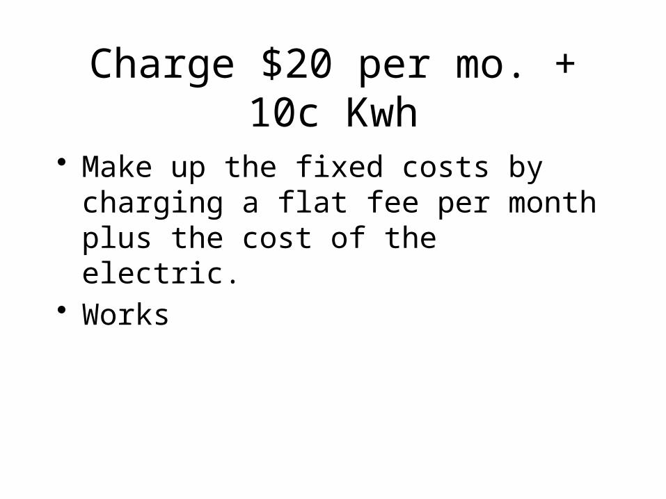
Charge $20 per mo. + 10c Kwh

• Make up the fixed costs by charging a flat fee per month plus the cost of the electric.

• Works

Politics (right wing interpretation)

• Voters want to make someone else pay.• Politicians call it concern for the poor.• Want to set electric rates to

– Load fixed costs on a small minority– Pay off powerful interests

Increasing Block Pricing

• First $115/MWH up to baseline• Then Higher price till 130 percent of

baseline usage• Then $410/MWH• The fixed costs get covered by the people

who buy the most, who are also the richest with the biggest pools.

Public Utilities Commission

• Covers costs• Overcharges minority of pool owners• Undercharges majority of renters• And the kicker….

– Has special rates for industry that are even lower than $115. Some ag rates where as low as $50.