Consumption-Based Asset Consumption-Based Asset Pricing After 25 YearsPricing After 25 Years

Douglas T. Breeden*Douglas T. Breeden*

*Dean and William W. Priest Professor of Finance, Duke University, Fuqua School of Business

Reference notes, tables and graphs for June 20, 2005 Western Finance Association Talk

2

Perspective and Goal of the PaperPerspective and Goal of the Paper

Rip Van Winkle (Austin Powers?) academic career: Intertemporal consumption, portfolio theory and asset pricing research 1976-1989. Left Duke 1992 to build Smith Breeden, did applied research on mortgages and corporate bonds. Returned to academia in 2000. Dean at Duke 2001-present, with usual IQ drop of Dean.

Paper will be a follow-up look at the numbers for some major results of consumption-based asset pricing that I began working on 25 years ago. There are many areas for future research that we’ll see.

3

Preceding Work on Intertemporal Preceding Work on Intertemporal Asset Pricing and the Term StructureAsset Pricing and the Term Structure Markowitz (1952), Sharpe (1964), Lintner (1965)

and Mossin (1966) developed diversification and the market-based CAPM.

Samuelson (1969), Merton (1969, 1971, 1973), Hakannson (1970), Fama (1970), Pye (1972) and Long (1975) pioneered intertemporal investments.

Hirshleifer (1970 book), Cox, Ingersoll and Ross (1985) and Garman (1976) on term structure.

4

First Decade of Selected Research on First Decade of Selected Research on Consumption-Based Asset PricingConsumption-Based Asset Pricing

Rubinstein (1976 BJEMS), Breeden-Litzenberger (1978 JB), Lucas (1978 Ec), Breeden (1979 JFE)

Hall (1978), Breeden (1980), Stulz (1981), Grossman-Shiller (1982) , Marsh-Rosenfeld (1982), Mankiw-Shapiro (1986), Mehra-Prescott (1985), Wheatley (1986), Hansen-Singleton (1982, 1983), Ferson (1983), Breeden (1984),Gibbons-Ferson.

Chen, Roll and Ross (1986), Grossman, Melino, Shiller (1987), Campbell-Shiller (1988), Breeden, Gibbons and Litzenberger(1989)

Term Structure: Garman (1976), Cox, Ingersoll, Ross (1985), Breeden (1986), Harvey (1988, 1989, 1991), Dunn-Singleton (1986), Sundaresan (1989)

5

Second Decade of Selected Research on Second Decade of Selected Research on Consumption-Based Asset PricingConsumption-Based Asset Pricing

Constantinides (1990), Abel (1990), Epstein-Zin(1991), Hansen-Jagannathan (1992), Cochrane(1991,1994,1996), Campbell (1991)

Campbell-Shiller(1990), Shanken (1990), Fama (1991), Kandel-Stambaugh(1991),Ferson-Constantinides (1991), Mankiw-Zeldes (1991), Fama-French (1992), Brennan-Schwartz-Lagnado(1997)

Heaton (1995), Elton-Gruber-Blake (1995), He-Modest (1995), Constantinides-Duffie (1996), Jagannathan-Wang (1996), Campbell-Cochrane (1999), Campbell-Viceira (1999), Ferson-Harvey(1999)

6

Third Decade of Selected Research on Third Decade of Selected Research on Consumption-Based Asset PricingConsumption-Based Asset Pricing

Campbell (2000), Heaton-Lucas (2000), Lettau-Ludwigson (2001a,b), Santos-Veronesi (2001),Brav-Constantinides-Geczy (2002), Wachter (2002), Barberis-Huang-Santos (2003)

Verdelhan (2003), Lustig-Verdelhan(2004), Piazzesi-Schneider-Tuzel (2003),Bansal-Yaron(2005), Bansal-Dittmar,Lundbad(2005),Bansal-Dittmar-Kiku (2004)

Jagannathan and Wang (2004), Parker-Julliard (2005), Campbell-Vuolteenaho (2004),Hansen-Heaton-Li(2005)

In total, 179 articles with “consumption, asset pricing” in the abstract, far more than mentioned here. Apologies.

7

Consumption Based Asset PricingConsumption Based Asset PricingOutline of PaperOutline of Paper

1. Consumption and marginal utility.2. Consumption risks of corporate profits & cash

flows. Capital budgeting.3. Consumption betas vs. market betas for industries.4. Term structure slope and consumption growth.5. Risk and return and the “Maximum Correlation

Portfolio” for consumption. 6. Consumption deviations from wealth and the

investment and income opportunity sets.7. Volatility of family consumption and the “Equity

Premium Puzzle.”

I.I. Consumption and Consumption and Marginal UtilityMarginal Utility

9

Consumption and Marginal UtilityConsumption and Marginal Utility

Some likely statistical indicators of times when the marginal utility of $1 is quite high, are the following:

1. Unemployment rate is increasing. 2. Job growth is less rapid than normal.

3. Businesses are failing more often, risky bonds’ yield spreads are high.

4. Banks are charging off more loans.

10

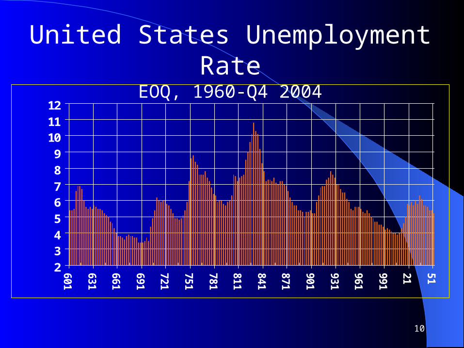
United States Unemployment RateEOQ, 1960-Q4 2004

23456789

101112

601

631

661

691

721

751

781

811

841

871

901

931

961

991

21 51

11

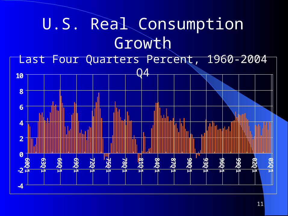
U.S. Real Consumption GrowthLast Four Quarters Percent, 1960-2004 Q4

-4

-2

0

2

4

6

8

10

60Q1

63Q1

66Q1

69Q1

72Q1

75Q1

78Q1

81Q1

84Q1

87Q1

90Q1

93Q1

96Q1

99Q1

02Q1

05Q1

12

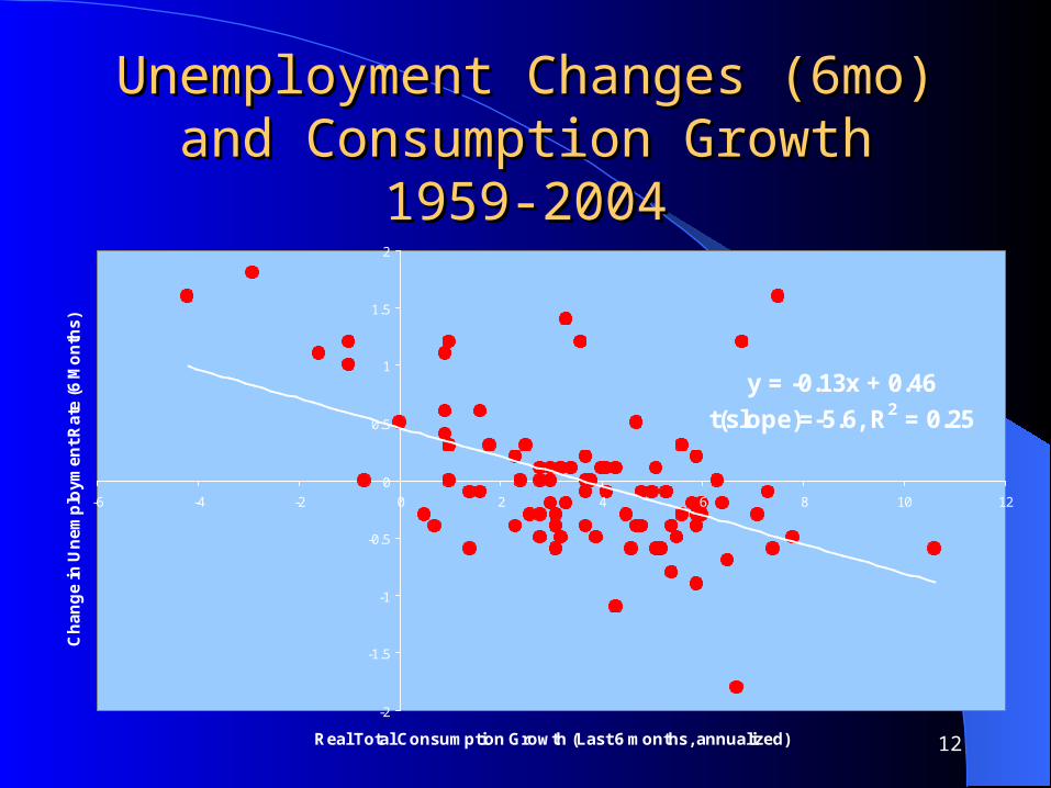
Unemployment Changes (6mo) and Unemployment Changes (6mo) and Consumption Growth 1959-2004Consumption Growth 1959-2004

y = -0.13x + 0.46

t(slope)=-5.6, R2 = 0.25

-2

-1.5

-1

-0.5

0

0.5

1

1.5

2

-6 -4 -2 0 2 4 6 8 10 12

Real Total Consumption Growth (Last 6 months, annualized)

Ch

an

ge

in U

ne

mp

loy

me

nt

Ra

te (

6 M

on

ths

)

13

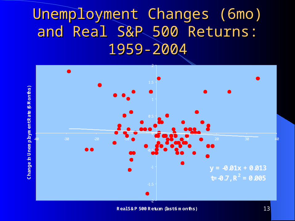
Unemployment Changes (6mo) and Unemployment Changes (6mo) and Real S&P 500 Returns: 1959-2004Real S&P 500 Returns: 1959-2004

y = -0.01x + 0.013

t=-0.7, R2 = 0.005

-2

-1.5

-1

-0.5

0

0.5

1

1.5

2

-40 -30 -20 -10 0 10 20 30 40

Real S&P 500 Return (last 6 months)

Ch

an

ge

in U

ne

mp

loy

me

nt

Ra

te (

6 M

on

ths

)

14

Unemployment Rate vs. Consumption Unemployment Rate vs. Consumption and Stock Prices and Stock Prices 1959-2004 (6 month changes)1959-2004 (6 month changes)

Independent

VariableSlope t-statistic CRSQ

S&P 500 -0.004 -0.65 -0.01

Total Real Consumption

-0.13 -5.56 0.25

NDS Consumption

-0.15 -4.58 0.18

15

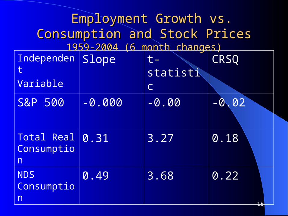
Employment Growth vs. Consumption Employment Growth vs. Consumption and Stock Prices and Stock Prices 1959-2004 (6 month changes)1959-2004 (6 month changes)

Independent

VariableSlope t-statistic CRSQ

S&P 500 -0.000 -0.00 -0.02

Total Real Consumption

0.31 3.27 0.18

NDS Consumption

0.49 3.68 0.22

16

Conclusion on Marginal UtilityConclusion on Marginal Utility

Consumption’s percentage changes likely represent more correctly changes in the marginal utility of $1 to individuals than do changes in real stock prices.

This is no failing of stock prices, for as the present value of future dividends, they should reflect future profit growth and changing risks and risk aversion.

II. Consumption and Market II. Consumption and Market Risks of Corporate Cash FlowsRisks of Corporate Cash Flows

18

Remember the Discounted Cash Remember the Discounted Cash Flow Approach to Valuation?Flow Approach to Valuation?

We teach our students to value an asset by discounting expected cash flows at their proper risk-adjusted discount rates.

Breeden-Litzenberger (Oct 1978, J. Business) derived risk-adjusted discount rates in a multiperiod economy with power utility, jointly lognormal cash flows. Correct discount rates were derived as the Consumption-based CAPM.

19

Consumption and Market Risks: Consumption and Market Risks: Earnings, Cash Flows vs. Stock PricesEarnings, Cash Flows vs. Stock Prices

Major problem applying CCAPM to stock prices is imprecision of consumption beta estimates vs. very precise market betas.

Breeden paper presented at the French Finance Ass’n at U. Paris Dauphine on “Capital Budgeting with Consumption” June 1989 showed opposite results for earnings risks. Updated slides follow. Consumption risks are more precisely estimated for earnings than are market risks, making CCAPM use natural for capital budgeting. Just in textbooks, e.g., Elton-Gruber.

20

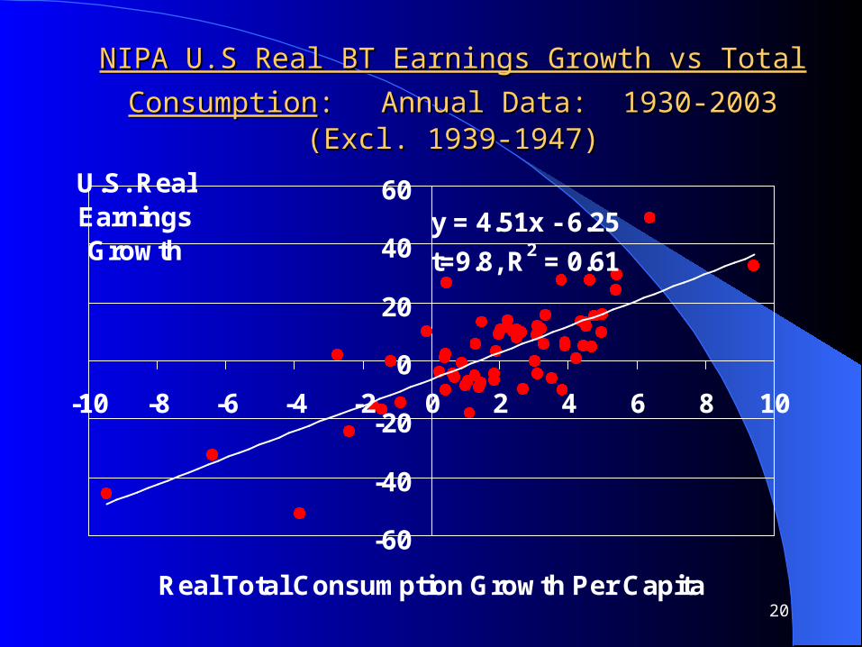
NIPA U.S Real BT Earnings Growth vs Total ConsumptionNIPA U.S Real BT Earnings Growth vs Total Consumption:: Annual Data: 1930-2003 (Excl. 1939-1947)Annual Data: 1930-2003 (Excl. 1939-1947)

y = 4.51x - 6.25

t=9.8, R2 = 0.61

-60

-40

-20

0

20

40

60

-10 -8 -6 -4 -2 0 2 4 6 8 10

Real Total Consumption Growth Per Capita

U.S. Real Earnings Growth

21

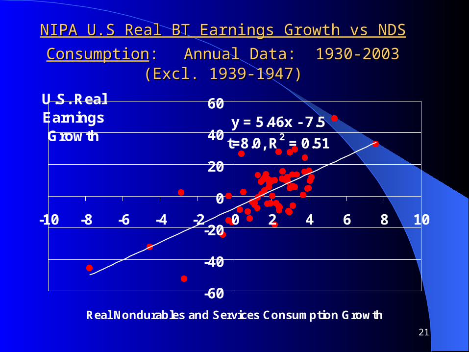
NIPA U.S Real BT Earnings Growth vs NDS ConsumptionNIPA U.S Real BT Earnings Growth vs NDS Consumption:: Annual Data: 1930-2003 (Excl. 1939-1947)Annual Data: 1930-2003 (Excl. 1939-1947)

y = 5.46x - 7.5

t=8.0, R2 = 0.51

-60

-40

-20

0

20

40

60

-10 -8 -6 -4 -2 0 2 4 6 8 10

Real Nondurables and Services Consumption Growth

U.S. Real Earnings Growth

22

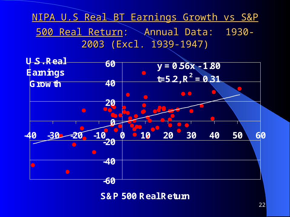
NIPA U.S Real BT Earnings Growth vs S&P 500 Real NIPA U.S Real BT Earnings Growth vs S&P 500 Real

ReturnReturn:: Annual Data: 1930-2003 (Excl. 1939-1947)Annual Data: 1930-2003 (Excl. 1939-1947)

y = 0.56x - 1.80

t=5.2, R2 = 0.31

-60

-40

-20

0

20

40

60

-40 -30 -20 -10 0 10 20 30 40 50 60

S&P 500 Real Return

U.S. Real Earnings Growth

23

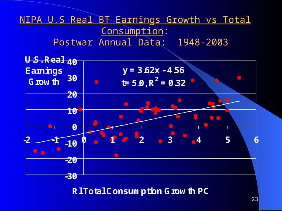
NIPA U.S Real BT Earnings Growth vs Total ConsumptionNIPA U.S Real BT Earnings Growth vs Total Consumption:: Postwar Annual Data: 1948-2003 Postwar Annual Data: 1948-2003

y = 3.62x - 4.56

t= 5.0, R2 = 0.32

-30

-20

-10

0

10

20

30

40

-2 -1 0 1 2 3 4 5 6

Rl Total Consumption Growth PC

U.S. Real Earnings Growth

24

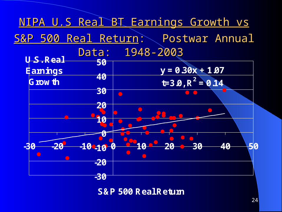
NIPA U.S Real BT Earnings Growth vs S&P 500 NIPA U.S Real BT Earnings Growth vs S&P 500

Real ReturnReal Return:: Postwar Annual Data: 1948-2003 Postwar Annual Data: 1948-2003

y = 0.30x + 1.07

t=3.0, R2 = 0.14

-30

-20

-10

0

10

20

30

40

50

-30 -20 -10 0 10 20 30 40 50

S&P 500 Real Return

U.S. Real Earnings Growth

25

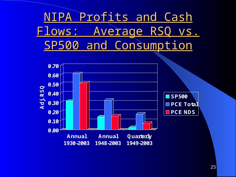
NIPA Profits and Cash Flows: NIPA Profits and Cash Flows: Average RSQ vs. SP500 and Average RSQ vs. SP500 and

ConsumptionConsumption

0.00

0.10

0.20

0.30

0.40

0.50

0.60

0.70

Ad

j. R

SQ

Annual1930-2003

Annual1948-2003

Quarterly1949-2003

SP500

PCE Total

PCE NDS

26

Conclusion on Cash Flow RisksConclusion on Cash Flow Risks

As we teach our students and in practice, it is both more correct and more intuitive to measure cash flow risks in terms of sensitivity to fluctuations in aggregate real consumption, rather than in terms of their relationship to stock market fluctuations.

Of course, if P/E multiples were constant, stock prices would be proportionate to earnings, and 1% higher earnings would give 1% higher stock prices. However, in reality, stocks’ price/earnings multiples fluctuate also with interest rates, economic risk and with growth prospects.

III. Relative Consumption Betas For III. Relative Consumption Betas For Industries Are Different From Industries Are Different From

Their Market BetasTheir Market Betas

28

Market Betas vs. Consumption Market Betas vs. Consumption Betas: Estimation ProcedureBetas: Estimation Procedure

Stock market betas are estimated from industry returns data from Professor Kenneth French’s website, using quarterly data from 1948-2004.

Consumption betas are from NIPA “coarse industries” quarterly profit data, using 2-quarter percentage changes in real profits. Actual calculation is of changes in real profits/employee compensation vs. real consumption growth, divided by average profits/employee compensation.

29

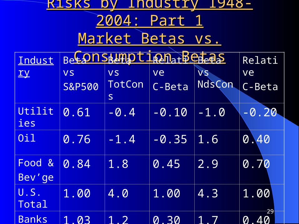
Risks by Industry 1948-2004: Part 1Risks by Industry 1948-2004: Part 1Market Betas vs. Consumption BetasMarket Betas vs. Consumption Betas

Industry Beta vs

S&P500

Beta vs TotCons

Relative

C-Beta

Beta vs NdsCon

Relative

C-Beta

Utilities 0.61 -0.4 -0.10 -1.0 -0.20

Oil 0.76 -1.4 -0.35 1.6 0.40

Food &

Bev’ge0.84 1.8 0.45 2.9 0.70

U.S. Total

1.00 4.0 1.00 4.3 1.00

Banks 1.03 1.2 0.30 1.7 0.40

30

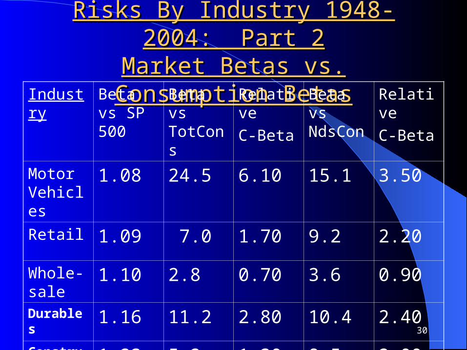
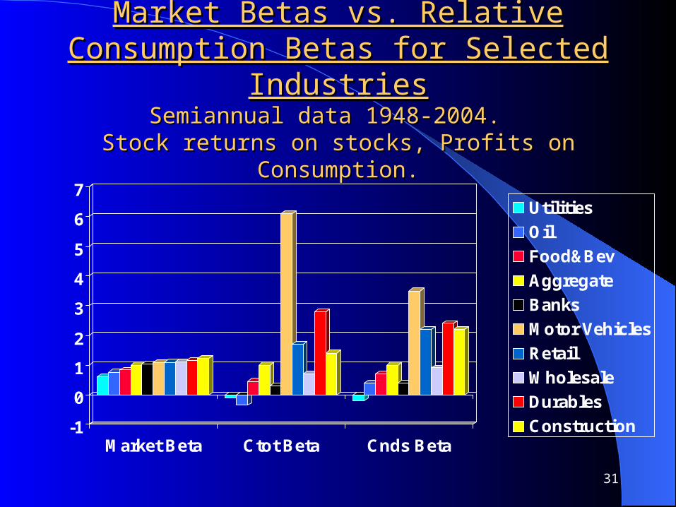
Risks By Industry 1948-2004: Part 2Risks By Industry 1948-2004: Part 2Market Betas vs. Consumption BetasMarket Betas vs. Consumption Betas

Industry Beta vs SP 500

Beta vs TotCons

Relative

C-Beta

Beta vs NdsCon

Relative

C-Beta

Motor Vehicles

1.08 24.5 6.10 15.1 3.50

Retail 1.09 7.0 1.70 9.2 2.20

Whole-sale

1.10 2.8 0.70 3.6 0.90

Durables 1.16 11.2 2.80 10.4 2.40

Construc-tion

1.23 5.2 1.30 8.5 2.00

31

Market Betas vs. Relative Consumption Market Betas vs. Relative Consumption Betas for Selected IndustriesBetas for Selected Industries

Semiannual data 1948-2004. Semiannual data 1948-2004. Stock returns on stocks, Profits on Consumption.Stock returns on stocks, Profits on Consumption.

-1

0

1

2

3

4

5

6

7

Market Beta Ctot Beta Cnds Beta

Utilities

Oil

Food&Bev

Aggregate

Banks

Motor Vehicles

Retail

Wholesale

Durables

Construction

IV. IV. The Term Structure of Interest Rates The Term Structure of Interest Rates as a Predictor of Economic Growthas a Predictor of Economic Growth

33

Theory: Slope of the Term Structure Optimally Theory: Slope of the Term Structure Optimally Related to Changes in Real Economic GrowthRelated to Changes in Real Economic Growth

Breeden’s (1986, JFE) article on “Consumption, Production, Inflation and Interest Rates: A Synthesis”, generalized Garman (1976), Rubinstein (1976), Fisher (1907) and Hirshleifer (1970) and derived and illustrated optimal relations of the term structure with expected consumption growth and its volatility.

Higher expected consumption growth is consistent with higher real rates. Higher volatility is consistent with lower real rates. With forecasted declines in expected growth, the term structure should have a negative slope. A positive slope should presage an expected strengthening in economic growth.

34

Tests and Uses of the Term Structure Slope Tests and Uses of the Term Structure Slope to Forecast Changes in Economic Growthto Forecast Changes in Economic Growth

Harvey (JFE 1988, 1989,1991,1993) tested Breeden’s equilibrium model and found it to be quite powerful, forecasting economic growth better than most professional economists and working in many countries.

Reflecting this research, in 1996, the slope of the term structure was added as a variable in the Index for Leading Economic Indicators.

Dotsey (1998) of the Federal Reserve Bank of Richmond found a negative term structure slope gave 18 true quarterly signals and only 2 false signals of recession in quarterly growth during the 1955-1995 period.

35

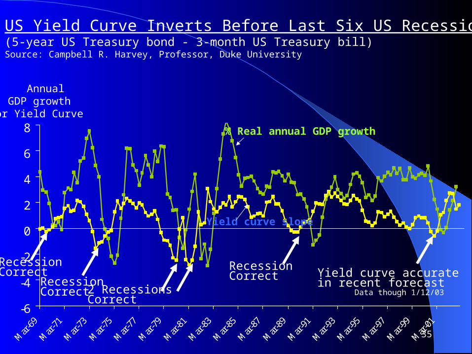
US Yield Curve Inverts Before Last Six US Recessions(5-year US Treasury bond - 3-month US Treasury bill)Source: Campbell R. Harvey, Professor, Duke University

-6

-4

-2

0

2

4

6

8 % Real annual GDP growth

Yield curve slope

RecessionCorrect 2 Recessions

Correct

RecessionCorrect Yield curve accurate

in recent forecast

RecessionCorrect

Annual GDP growthor Yield Curve

Data though 1/12/03

36

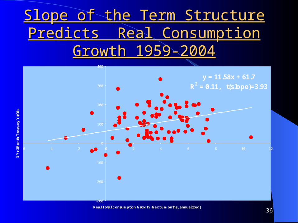
Slope of the Term Structure Predicts Slope of the Term Structure Predicts Real Consumption Growth 1959-2004Real Consumption Growth 1959-2004

y = 11.58x + 61.7

R2 = 0.11, t(slope)=3.93

-300

-200

-100

0

100

200

300

400

-6 -4 -2 0 2 4 6 8 10 12

Real Total Consumption Growth (Next 6 months, annualized)

3 Y

r-3M

on

th T

reas

ury

Yie

lds

37

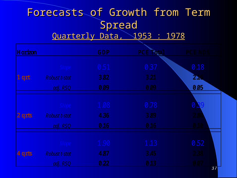
Forecasts of Growth from Term SpreadForecasts of Growth from Term SpreadQuarterly Data, 1953 : 1978Quarterly Data, 1953 : 1978

Horizon GDP PCE Total PCE NDS

Slope 0.51 0.37 0.181 qrt Robust t-stat 3.82 3.21 2.16

adj. RSQ 0.09 0.09 0.05

Slope 1.08 0.78 0.392 qrts Robust t-stat 4.36 3.89 2.80

adj. RSQ 0.16 0.16 0.10

Slope 1.90 1.13 0.524 qrts Robust t-stat 4.87 3.45 2.38

adj. RSQ 0.22 0.13 0.07

38

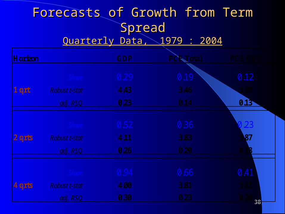
Forecasts of Growth from Term SpreadForecasts of Growth from Term SpreadQuarterly Data, 1979 : 2004Quarterly Data, 1979 : 2004

Horizon GDP PCE Total PCE NDS

Slope 0.29 0.19 0.121 qrt Robust t-stat 4.43 3.46 3.59

adj. RSQ 0.23 0.14 0.13

Slope 0.52 0.36 0.232 qrts Robust t-stat 4.11 3.83 3.87

adj. RSQ 0.26 0.20 0.18

Slope 0.94 0.66 0.414 qrts Robust t-stat 4.00 3.81 3.61

adj. RSQ 0.30 0.23 0.20

39

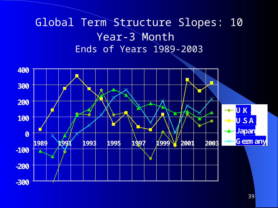
Global Term Structure Slopes: 10 Year-3 Month Ends of Years 1989-2003

-300

-200

-100

0

100

200

300

400

1989 1991 1993 1995 1997 1999 2001 2003

U.K.U.S.A.JapanGermany

V. Consumption Risk and Returns and V. Consumption Risk and Returns and the Maximum Correlation Portfoliothe Maximum Correlation Portfolio

41

Maximum Correlation Portfolio ElementsMaximum Correlation Portfolio ElementsS&P 500, Baa-Treasury Bonds, Term SpreadS&P 500, Baa-Treasury Bonds, Term Spread

Breeden, Gibbons and Litzenberger (JF, 1989) proved that the CCAPM also holds with regard to betas measured against the maximum correlation portfolio for consumption.

Three broad traded markets are for (1) stocks, (2) Government bonds and (3) corporate bonds. Consumption relates to each of these through effects of wealth, the term structure, and relation of credit risk to the economic cycle, respectively.

42

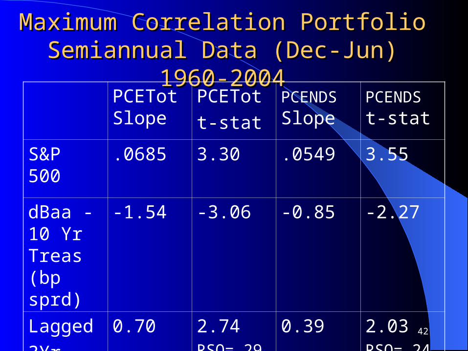
Maximum Correlation PortfolioMaximum Correlation PortfolioSemiannual Data (Dec-Jun) 1960-2004Semiannual Data (Dec-Jun) 1960-2004

PCETot Slope

PCETot

t-stat

PCENDS Slope

PCENDS t-stat

S&P 500 .0685 3.30 .0549 3.55

dBaa -10 Yr Treas (bp sprd)

-1.54 -3.06 -0.85 -2.27

Lagged

3Yr-3MoTS Slope

0.70 2.74RSQ=.29

0.39 2.03RSQ=.24

““Consumption Risk and the Cross-Section of Consumption Risk and the Cross-Section of Expected Returns”,Expected Returns”, Parker-Julliard (JPE, 2005)Parker-Julliard (JPE, 2005)

Consumption betas measured by contemporaneous covariances of assets’ returns and consumption growth, fail to explain the dispersion in risk premiums across assets.

Parker-Julliard measure ultimate consumption risk as covariation of return with current and future consumption growth. Ultimate consumption betas, therefore, measure the exposure of asset returns to long-run risks in consumption.

Consumption Risk and Expected ReturnsConsumption Risk and Expected ReturnsParker-Julliard (JPE, 2005) continuedParker-Julliard (JPE, 2005) continued

Parker-Julliard argue that ultimate consumption risk measures are much more robust to measurement errors in consumption, as well as slow and costly adjustments of consumption to returns.

Using post-war quarterly data on 25 Fama-French portfolios sorted by Book Equity/Market Equity and Size, they show ultimate consumption risk measures are able to explain from 44% to 73% of the variation in expected returns.

VI. VI. Consumption Deviations from Wealth Consumption Deviations from Wealth as a Predictor of Income and Investment as a Predictor of Income and Investment

OpportunitiesOpportunities

46

Consumption Deviations from Wealth Predict Consumption Deviations from Wealth Predict Income and Investment OpportunitiesIncome and Investment Opportunities

Breeden (1984, JET) showed with relative risk aversion >1, investors’ consumption levels are positively related to income and investment opportunities. (If RRA<1, reverse hedging occurs.)

In June 1989, at the French Finance Association in Paris and in 1991 at Harvard, Breeden paper on “Capital Budgeting with Consumption”, argued that as consumption optimally is a function of wealth, income and investment opportunities, consumption fluctuations orthogonalized for wealth effects should be indicators of the income and investment opportunity set. Test results presented then are updated as follows:

47

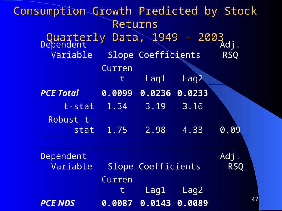
Consumption Growth Predicted by Stock ReturnsConsumption Growth Predicted by Stock ReturnsQuarterly Data, 1949 – 2003Quarterly Data, 1949 – 2003

Dependent Variable Slope Coefficients

Adj.RSQ

  Current Lag1 Lag2  

PCE Total 0.0099 0.0236 0.0233  

t-stat 1.34 3.19 3.16  

Robust t-stat 1.75 2.98 4.33 0.09

Dependent Variable Slope Coefficients

Adj. RSQ

  Current Lag1 Lag2  

PCE NDS 0.0087 0.0143 0.0089  

t-stat 2.05 3.35 2.08  

Robust t-stat 2.54 3.58 2.66 0.08

48

Consumption Growth Deviations and the Consumption Growth Deviations and the Income and Investment Opportunity SetIncome and Investment Opportunity Set

The lagged values of the residuals from the above regressions are examined for predictive ability with regard to income, wages and corporate profits.

Specifically, we regress the growth rate of each variable on its own lag and the lagged consumption residuals.

49

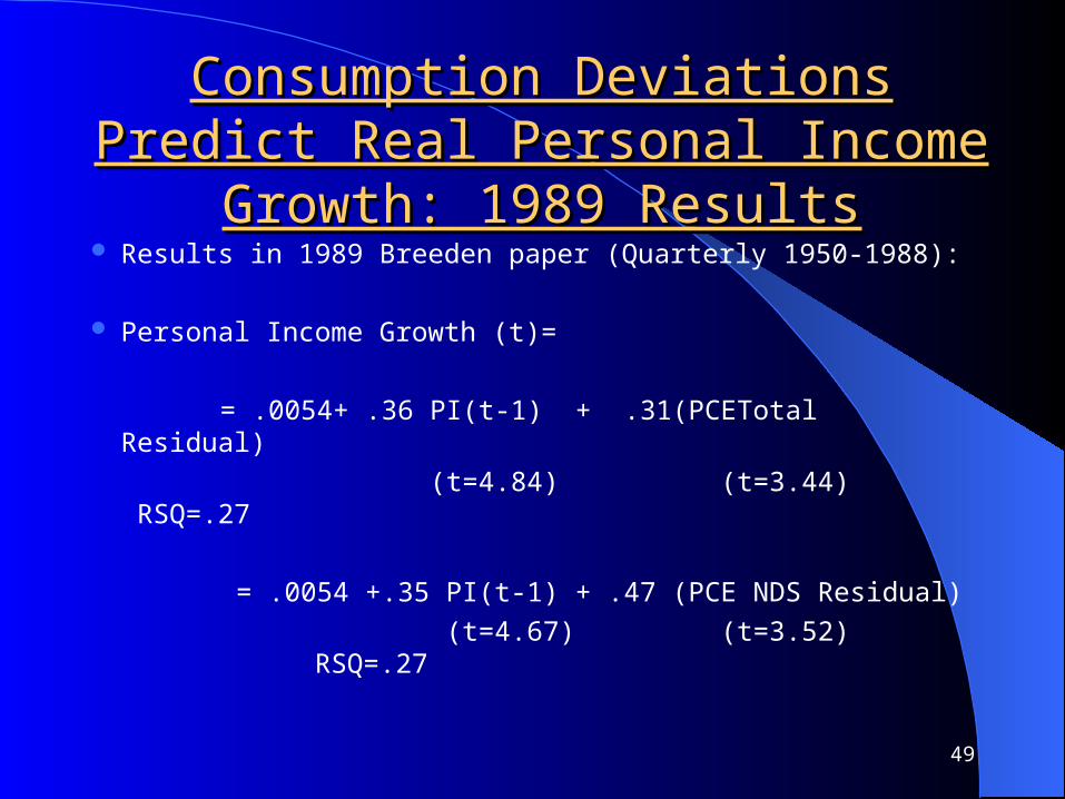
Consumption Deviations Predict Real Consumption Deviations Predict Real Personal Income Growth: 1989 ResultsPersonal Income Growth: 1989 Results Results in 1989 Breeden paper (Quarterly 1950-1988):

Personal Income Growth (t)=

= .0054+ .36 PI(t-1) + .31(PCETotal Residual)

(t=4.84) (t=3.44) RSQ=.27

= .0054 +.35 PI(t-1) + .47 (PCE NDS Residual)

(t=4.67) (t=3.52) RSQ=.27

50

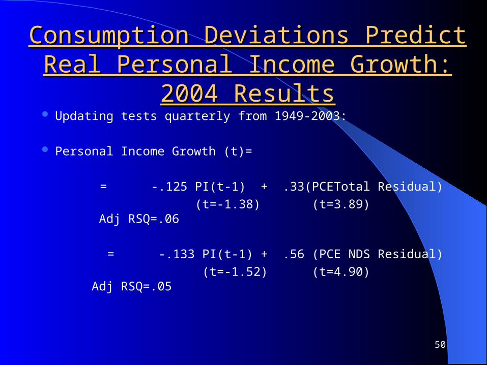
Consumption Deviations Predict Real Consumption Deviations Predict Real Personal Income Growth: 2004 ResultsPersonal Income Growth: 2004 Results Updating tests quarterly from 1949-2003:

Personal Income Growth (t)=

= -.125 PI(t-1) + .33(PCETotal Residual)

(t=-1.38) (t=3.89) Adj RSQ=.06

= -.133 PI(t-1) + .56 (PCE NDS Residual)

(t=-1.52) (t=4.90) Adj RSQ=.05

51

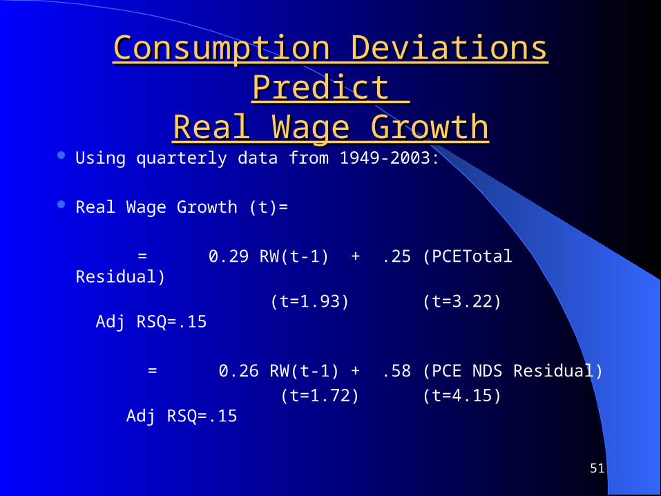
Consumption Deviations Predict Consumption Deviations Predict Real Wage GrowthReal Wage Growth

Using quarterly data from 1949-2003:

Real Wage Growth (t)=

= 0.29 RW(t-1) + .25 (PCETotal Residual)

(t=1.93) (t=3.22) Adj RSQ=.15

= 0.26 RW(t-1) + .58 (PCE NDS Residual)

(t=1.72) (t=4.15) Adj RSQ=.15

52

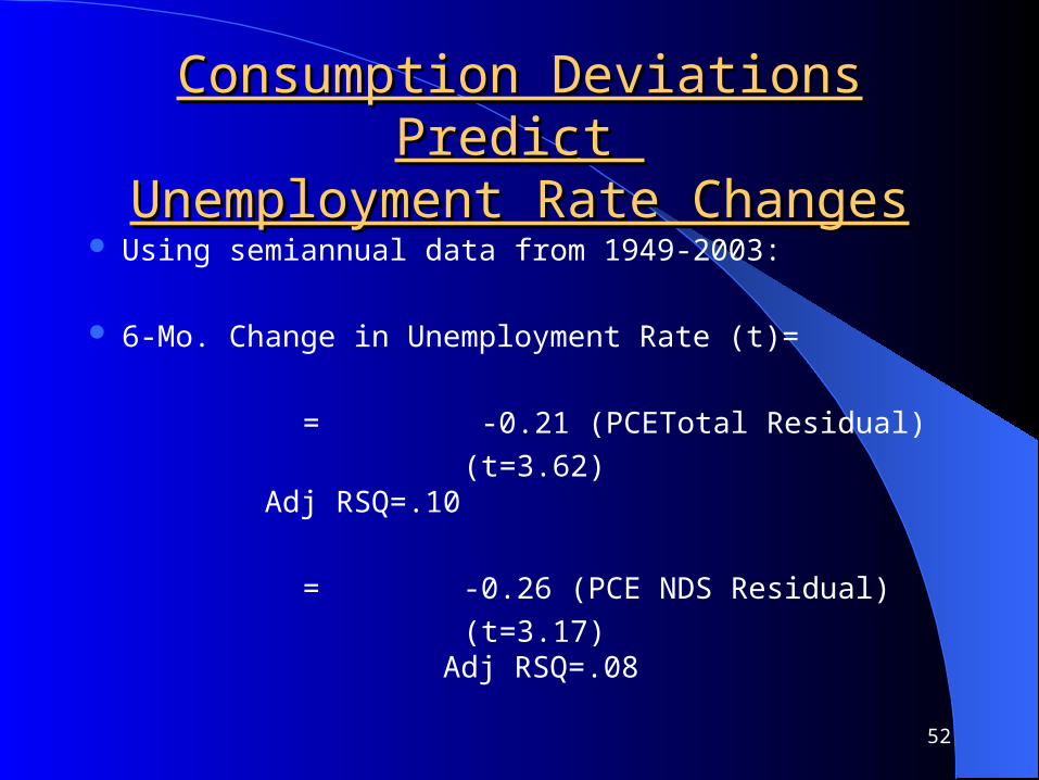
Consumption Deviations Predict Consumption Deviations Predict Unemployment Rate ChangesUnemployment Rate Changes

Using semiannual data from 1949-2003:

6-Mo. Change in Unemployment Rate (t)=

= -0.21 (PCETotal Residual)

(t=3.62) Adj RSQ=.10

= -0.26 (PCE NDS Residual)

(t=3.17) Adj RSQ=.08

53

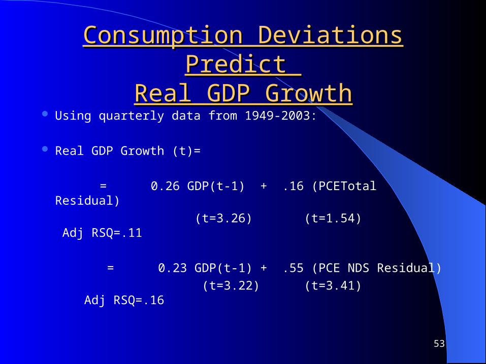
Consumption Deviations Predict Consumption Deviations Predict Real GDP GrowthReal GDP Growth

Using quarterly data from 1949-2003:

Real GDP Growth (t)=

= 0.26 GDP(t-1) + .16 (PCETotal Residual)

(t=3.26) (t=1.54) Adj RSQ=.11

= 0.23 GDP(t-1) + .55 (PCE NDS Residual)

(t=3.22) (t=3.41) Adj RSQ=.16

54

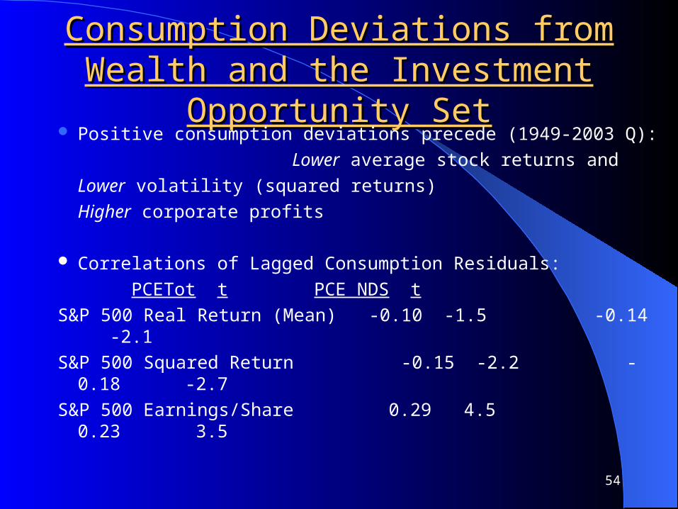
Consumption Deviations from Wealth Consumption Deviations from Wealth and the Investment Opportunity Setand the Investment Opportunity Set

Positive consumption deviations precede (1949-2003 Q):

Lower average stock returns and

Lower volatility (squared returns)

Higher corporate profits

Correlations of Lagged Consumption Residuals:

PCETot t PCE NDS t

S&P 500 Real Return (Mean) -0.10 -1.5 -0.14 -2.1

S&P 500 Squared Return -0.15 -2.2 -0.18 -2.7

S&P 500 Earnings/Share 0.29 4.5 0.23 3.5

55

Conclusion on Consumption and the Conclusion on Consumption and the Income and Investment Opportunity SetsIncome and Investment Opportunity Sets

Test results show strongly that, as consumption and portfolio theory predict, consumption choices do reflect knowledge about future income and investment opportunities.

High consumption relative to wealth is followed by high wage and personal income growth, and by higher corporate profits and reduced volatility of investment returns. Low consumption/wealth reflects weak income opportunities, lower profits and higher risks. Lettau-Ludwigson’s (2001a,b) results confirm some of these effects.

V.V. Volatility of Individual Consumption Volatility of Individual Consumption vs. Aggregate Consumption and the vs. Aggregate Consumption and the

Equity Premium PuzzleEquity Premium Puzzle

See also: Heaton-Lucas (1996 JPE) and

Brav, Constantinides, Geczy (2002 JPE)

57

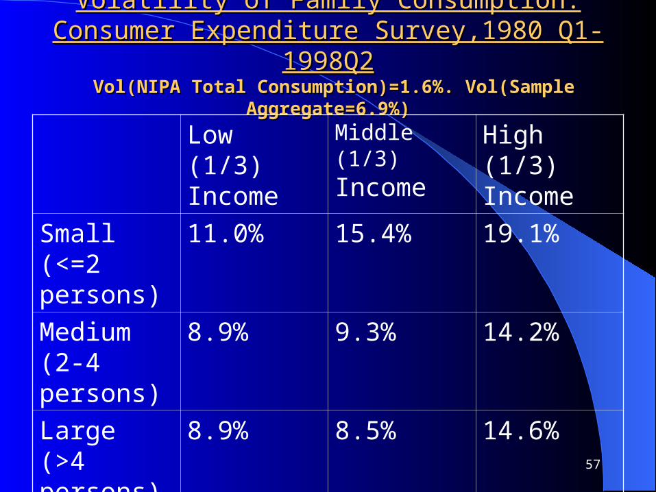
Volatility of Family Consumption: Consumer Volatility of Family Consumption: Consumer Expenditure Survey,1980 Q1-1998Q2Expenditure Survey,1980 Q1-1998Q2

Vol(NIPA Total Consumption)=1.6%. Vol(Sample Aggregate=6.9%)Vol(NIPA Total Consumption)=1.6%. Vol(Sample Aggregate=6.9%)

Low (1/3) Income

Middle (1/3) Income

High (1/3) Income

Small (<=2 persons)

11.0% 15.4% 19.1%

Medium (2-4 persons)

8.9% 9.3% 14.2%

Large (>4 persons)

8.9% 8.5% 14.6%

58

Equity Premium Puzzle and Equity Premium Puzzle and Consumption VolatilityConsumption Volatility

Individual consumption volatility is 5-10 times larger than measured volatility of NIPA aggregate consumption. High income individuals own the most assets, have highest consumption volatility.

Reasons include incomplete markets and optimal incentives for labor choices.

Marginal utility is indeed related to that consumption volatility and likely helps explain the equilibrium equity risk premium.