contact and friction simulation for computer graphics
TRANSCRIPT

Contact and Friction Simulation for ComputerGraphics
SHELDON ANDREWS, École de technologie supérieure, CanadaKENNY ERLEBEN, University of Copenhagen, Denmark
Efficient simulation of contact is of interest for numerous physics-based animation applications. Forinstance, virtual reality training, video games, rapid digital prototyping, and robotics simulation are allexamples of applications that involve contact modeling and simulation. However, despite its extensiveuse in modern computer graphics, contact simulation remains one of the most challenging problems inphysics-based animation.This course covers fundamental topics on the nature of contact modeling and simulation for computer
graphics. Specifically, we provide mathematical details about formulating contact as a complementarityproblem in rigid body and soft body animations. We briefly cover several approaches for contactgeneration using discrete collision detection. Then, we present a range of numerical techniques forsolving the associated LCPs and NCPs. The advantages and disadvantages of each technique are furtherdiscussed in a practical manner, and best practices for implementation are discussed. Finally, we concludethe course with several advanced topics, such as anisotropic friction modeling and proximal operators.Programming examples are provided on the course website to accompany the course notes.
CCS Concepts: • Computing methodologies→ Simulation by animation; Physical simulation;Real-time simulation; • Applied computing→ Physics.
Permission to make digital or hard copies of part or all of this work for personal or classroom use is grantedwithout fee provided that copies are not made or distributed for profit or commercial advantage and that copiesbear this notice and the full citation on the first page. Copyrights for third-party components of this work mustbe honored. For all other uses, contact the owner/author(s).SIGGRAPH ’21 Courses, August 09-13, 2021, Virtual Event, USA© 2021 Copyright held by the owner/author(s).ACM ISBN 978-1-4503-8361-5/21/08.https://doi.org/10.1145/3450508.3464571
1

SIGGRAPH ’21 Courses, August 09-13, 2021, Virtual Event, USA Andrews and Erleben
Additional Key Words and Phrases: contact, friction, complementarity problems, Newton methods,iterative methods, pivoting methods, splitting methods, physics-based animation
ACM Reference Format:Sheldon Andrews and Kenny Erleben. 2021. Contact and Friction Simulation for Computer Graphics. InSpecial Interest Group on Computer Graphics and Interactive Techniques Conference Courses (SIGGRAPH’21 Courses), August 09-13, 2021. ACM, New York, NY, USA, 124 pages. https://doi.org/10.1145/3450508.3464571
Contents
Abstract 1Contents 2Preface 5Syllabus 71 Introduction to Contact Simulation 81.1 The Equations of Motion 91.2 Time Integration 91.3 Constraints 111.4 Non-interpenetration Contact Constraint 131.4.1 Non-interpenetration Jacobian 151.4.2 Non-interpenetration Constraint for Soft Bodies 161.5 The Coulomb Friction Law 171.5.1 Theory of Friction 191.6 The Linear Complementarity Problem Model of Frictional Contact 231.7 The Boxed Linear Complementarity Problem Model of Frictional Contact 281.8 The Cone Complementarity Problem for Frictional Contact 291.9 Constraint Stabilization 321.10 Soft vs. Rigid Body 341.10.1 Assembling the Matrices for a Rigid Body System 341.10.2 Assembling the Matrices for a Soft Body System 372 Contact Generation 402.1 Analytic Shapes 412.1.1 Sphere-Sphere Intersection 422.1.2 Sphere-OBB Intersection 422.1.3 OBB-OBB Intersection 442.2 Mesh-based Representations 472.2.1 Continuous Collision Detection of Mesh Features 482.2.2 Continuous Collision Detection of Face-Vertex Pair 502.2.3 Continuous Collision Detection of Edge-Edge Pair 512.3 Signed Distance Fields 52
2

Contact and Friction Simulation SIGGRAPH ’21 Courses, August 09-13, 2021, Virtual Event, USA
2.3.1 SDF-Point Intersection 532.3.2 SDF-Mesh Intersection 542.3.3 Implementation Notes 553 Numerical Methods 573.1 Pivoting Methods 573.1.1 Incremental Pivoting 593.1.2 Principal Pivoting Methods 603.1.3 Block Principal Pivoting 623.1.4 Implementation Notes 623.2 Fixed-point methods 633.2.1 Splitting Methods 643.2.2 Extending to the BLCP 703.2.3 Ordering of Variables 713.2.4 The Blocked Gauss-Seidel Method 723.2.5 Staggering 763.2.6 The Projected Gauss-Seidel Subspace Minimization Method 763.2.7 The Non-Smooth Nonlinear Conjugate Gradient Method 773.3 Non-Smooth Newton Methods 803.3.1 Minimum-Map Formulation 833.3.2 Fischer-Burmeister Formulation 833.3.3 Friction 843.3.4 Newton’s Method 853.3.5 Preconditioning 854 Selected Topics 874.1 Proximal Operators 874.1.1 The Proximal Operator Model 894.1.2 Iterative Methods for the Fixed-Point Scheme 954.1.3 Closest Point on Ellipsoid 974.1.4 The 𝑟 -Factor Strategies 1004.1.5 Time-Stepping Methods 1034.1.6 Constraint Stabilization by Post-step Projection 1044.2 Anisotropic Friction 1054.2.1 Friction Cone Modeling 1064.2.2 The Matchstick Model 1074.2.3 Fixed-point Solvers 1094.2.4 LCP-based Solvers 1104.2.5 NCP-based Solvers 1114.2.6 Implementation Notes 1124.3 Penalty Methods 1134.3.1 Rigid Bodies 113
3

SIGGRAPH ’21 Courses, August 09-13, 2021, Virtual Event, USA Andrews and Erleben
4.3.2 Soft Bodies 1154.3.3 Implementation Notes 1154.3.4 Penalty Based Friction 1164.3.5 Other Penalty Methods 117References 120
4

Contact and Friction Simulation SIGGRAPH ’21 Courses, August 09-13, 2021, Virtual Event, USA
PREFACEWhy a SIGGRAPH course on contact and friction simulation? The answer, quite simply, is thatit is an important topic. As a classic problem in physics-based animation, contact simulationhas been the focus on many scientific works over the past several decades in computer graphics.Furthermore, there is a demand for friendly teaching material about the topic since it is difficultto approach for non-specialists.Contact and friction simulation in computer graphics field has evolved a lot since the 1980s.
During this time, a lot of effort has gone into uncovering fast and robust methods, and utilizinghardware such as GPUs. The performance and robustness of these methods now enablestechniques developed in computer graphics to be deployed into other fields. For instance,robotics and medical simulation are two fields where computer graphics simulations arenow pushing the limits of the state-of-the-art. Digital prototyping, learning and training areother important application contexts, and there is still a need for advances here. Currently,differentiable physics, rich friction models, machine learning-based physics, soft-rigid andsoft-soft body contact are open topics that the research community is pursuing. We hope thesenotes will give the next generation of researchers the necessary foundation to begin solvingthese challenges.These course notes have been assembled over a period of a couple of years. Topics have
been introduced and pulled out continuously in this process, and we will likely continue to doso in future versions of these course notes. A few topics kept coming back to us as being morefundamental, in that they form the foundation for understanding a lot of recent work in thefield. Hence, this material makes up the core of the course notes, and they are mainly aboutunderstanding the physical models and numerical methods. By that we mean the mathematicalequations we write up when we describe the models, along with the methods we apply tocompute solutions for our models. Ideally, we try to keep models and methods separate, as theyshould be. Historically, a huge part of the field is devoted to fast and robust numerical methods,and in particular constraint-based approaches, such as the ones based on complementarityproblem formulations, make up a big part of the picture. Therefore, we devote a lot of effort togive a firm understanding of this popular approach.It is impossible to cover all topics related to contact and friction simulation in a three-hour
SIGGRAPH course, and we had to cut out many topics in order to remain relatively concise.For instance, in this version of the course we ignore impulse-based methods that use collisionlaws and event propagation. The coverage of collision detection is also limited to just theprincipled ideas of how to generate contact points for common shape representations. Othercompromises include restricting the presentation of penalty-based methods to focus on explicittime schemes. Also, recent work on continuous time integration and normals is omitted, as wellas work on barrier methods. However, we do introduce the cone-complementarity problemformulation for modeling contact and friction, as these are a recent very interesting additionto the field, yet only brief details about the numerical methods related to this type of model
5

SIGGRAPH ’21 Courses, August 09-13, 2021, Virtual Event, USA Andrews and Erleben
are covered. Lastly, we do not cover position-based and projective dynamics directly. However,solvers applied here bear a resemblance to the proximal operators and iterative solvers, whichwe do cover in full details. There is a bundle of more work that deserves mentioning here, andwe apologize for not having the time and space to give the wonderful work on those topicsthe attention they deserve.We would like to acknowledge that a lot of people have been involved in the creation of
these course notes. A community of peers has helped us to generate ideas and discussion howto best present and explain topics, given feedback, proofread the content at various stages ofdevelopment, pointed us to relevant work in the field, and much more. The list is long, but inparticular we would like to acknowledge the support and help from Miles Macklin, Paul G.Kry, Mihai Francu, Eric Paquette and many others.Finally, we hope that you will enjoy this course, and that you find contact and friction
simulation a fun topic to learn about! Please visit the course website siggraphcontact.github.io,where you will find programming examples and other supplementary material related to thesenotes.
Sheldon and Kenny
6

Contact and Friction Simulation SIGGRAPH ’21 Courses, August 09-13, 2021, Virtual Event, USA
SYLLABUSIntroduction to Contact Simulation. We introduce the idea of time stepping a simulation.The update loop can contain a time integrator, a numerical solver to compute implicit forcesor constraints, and a collision detection routine. We present the ordinary differential equations(ODE) that govern the Newton dynamics of a simulation. Stepping in time an ODE is done usingan integrator and we introduce the semi-implicit and implicit Euler methods with a focus onstability. A Lagrangian perspective permits us to easily add kinematic or geometric constraintsthrough Lagrange multipliers. We demonstrate that in this framework, non-interpenetration isrealized as a unilateral constraint, which is imposed by defining a gap function between bodies.Imposing such constraints requires impulsive forces that vanish when contact breaks, andwe explain how this naturally leads to the complementarity conditions. Due to discretization,errors in the constraints can accumulate resulting in penetration artefacts. This is especiallytrue for acceleration or velocity formulations. A standard remedy is to use stabilization, suchas Baumgarte.Contact Generation. In this section, we focus on the practicalities of how to generate
contacts. We introduce the idea of generating contact based on primitive geometric features,signed distance fields. The primary focus is on guidelines for robust contact detection andextracting the contact information from various surface representations, and the variousproblems that can arise.Numerical Methods. We focus on the underlying mathematical derivation and recast the
physical model into a problem that can be solved using various numerical techniques. We firstshow how pivoting methods may be used to solve the contact LCP by estimating the index setof simulation variables. We then introduce the fixed point methods as framework for solvinggeneral non-linear models, and proceed to derive the PGS, SOR, and Jacobi methods whichare a popular solvers for interactive computer graphics applications. Finally, we reformulatethe problem of satisfying the contact conditions and equations of motion as a root searchproblem, providing the the basis for Newton-type methods, such as minimum-map and Fischer-Burmeister reformulations. We also cover aspects of the importance of proper preconditioningand regularization to achieve fast performance and robustness.Selected Topics. We present on recent work for modeling friction cones that captures the
anisotropic nature of certain materials. We also present some special considerations whensimulating frictional contact using penalty-based methods.
7

SIGGRAPH ’21 Courses, August 09-13, 2021, Virtual Event, USA Andrews and Erleben
1 INTRODUCTION TO CONTACT SIMULATIONContact simulation is mainly concerned with computing the forces that exist at interfacesbetween physical objects. Physical objects can range from rigid bodies, such as a billiard ballor vehicle chassis, to soft bodies, such as cloth and hair. We simply refer to a collection of suchobjects and the forces acting on them and between them as a physical system. The interfaceforces are termed contact forces and they prevent objects from penetrating each other duringmotion and deformation, and they additionally model the resistance due to objects againsteach other. These course notes are primarily focused on how to model and compute contactforces in an efficient and robust manner.Historically, constraint based methods for computing contact forces have been used by the
graphics community for simulation of rigid bodies. Many earlier works focused on improvingperformance by developing faster methods for rigid body simulations. Hence, a lot of thenotation we use in these notes are influenced by these early works. One might primarilyread these notes while thinking about contact between rigid bodies, and indeed many of theexamples demonstrate the rigid case as it is the easier case after all. Nevertheless, much of thematerial we cover here applies to elastic models and soft bodies too, and we will address someof these differences when they arise. Furthermore, a complicating factor in contact simulationis the generation of contacts using collision detection, which is a topic that we cover briefly inorder to convey the principal ideas.At a high-level, there are three main paradigms for contact simulation. First, contact may be
simulated by constraint based methods, and these course notes are rooted in this paradigm.This paradigm bares a lot of resemblance to constrained optimization where constraints aresolved exactly. Another paradigm is penalty based approaches, and these tend to rely on force-based modeling to resolve interpenetration at the interface. Often this paradigm is introducedconceptually as small abstract springs working between objects to keep them from overlapping.Hence, the springs "penalize" overlap which gives rise to the name for this class of methods.There are similarities here to penalty methods in numerical optimization, in particular barriermethods that have recently become popular for contact simulation. The last paradigm accountsfor impulse-based methods where the contact between objects is conceptualized as sequencesof micro-collisions. These notes take their outset in the constraint based approaches as thesehave been dominating real-time interactive simulation for decades. Constraint-based methodsalso have the nice property that they are able to guarantee solving for contact exactly, at leastin such a way that constraints are always fulfilled. However, we later explain formulationsbased on penalty methods and explain best practices when using this class of approach formodeling contact in simulation pipelines. 6These course notes seek to not only give the reader intuition about the theoretical models
that are used as the basis for a wide variety of contact simulations, but also to highlightsome best practices for all stages of the simulation pipeline. Note that the “An Introductionto Physics-Based Animation” SIGGRAPH course [Bargteil et al. 2020] is an excellent related
8

Contact and Friction Simulation SIGGRAPH ’21 Courses, August 09-13, 2021, Virtual Event, USA
reference for an in-depth discussion of preliminaries, while this course on contact and frictionnaturally picks up from where the other course wraps up.We begin by introducing the equations of motion and numerical integration by time
stepping. Then, kinematic constraints are derived to resolve non-interpenetration and weexplain the importance of the complementarity condition. This leads into a presentation ofCoulomb friction and how it is included in the formulation of the contact problem. Finally,the introduction ends with a discussion on how the formulation may be adapted to soft bodysimulations.
1.1 The Equations of MotionThe Newton-Euler equations of motion [Goldstein et al. 2002] that govern the dynamics of aphysical system form a second-order ODE that can be written as
M(𝑡) ¤u(𝑡) = f (q(𝑡), u(𝑡), 𝑡) , (1)
whereM(𝑡) are themasses, q(𝑡) are the generalized positions, u(𝑡) are the generalized velocities,and f (𝑡, q(𝑡), u(𝑡)) are the generalized forces acting on the system, which depend on thepositions and velocities. Notice that we are agnostic about what we are simulating at this point,and the equation can be seen as describing the motion of rigid bodies, thin shells, or elasticsolids. Also notice that all terms in Equation 1 depend on the time 𝑡 . However, in computergraphics, we are often only interested in determining the dynamical behavior at a particularinstant in time, and so the Newton-Euler equations may be written more succinctly as
M ¤u = f . (2)
The time instants for evaluating Equation 2 are determined by a numerical integrator, andin the next section we briefly outline how to “step” the equations of motion using a popularintegration method in computer graphics.
1.2 Time IntegrationPhysical simulations for computer graphics are typically performed using a discrete numericalintegration with time step ℎ. There are two main types of numerical integrators: explicit andimplicit. The former evaluate the force at the beginning of the time step f (q−, u−), while thelatter evaluate it at the end f (q+, u+). Note that the superscript □+ is used to indicate an implicitquantity and □− an explicit quantity. We can denote the forces for now simply as f withoutspecifying whether they are implicit or explicit, and this particular choice will depend uponthe application context. However, we will drop the latter from here on since computer graphicsapplications largely use implicit integration schemes due to their increased numerical stability.A Taylor expansion of the implicit velocities gives the first-order approximation
u+ ≈ u + ℎ ¤u ,
9

SIGGRAPH ’21 Courses, August 09-13, 2021, Virtual Event, USA Andrews and Erleben
where the change in velocities from the start of the time step to the end of the time step isdetermined by the accelerations ¤u. Using this approximation to substitute for the accelerationsin Equation 2, and by applying a simple Euler integration scheme, we can write the linearrelationship governing the motion of a system with 𝑛 degrees freedom at each time step as
Mu+ = Mu + ℎ f (3)
with the mass matrix M ∈ R𝑛×𝑛, the momentum term Mu ∈ R𝑛 and applied forces f ∈ R𝑛.Here, the velocities u+ ∈ R𝑛 are determined at the end of the time step, and for simplicity wewill consider the mass matrix M to be constant over the time step. For a rigid body system,the mass matrix will consist of small blocks containing the total mass of the rigid bodies andtheir 3 × 3 inertia tensors, whereas for soft bodies the mass matrix can be given by a volumeintegral of mass density over some elements or a diagonal matrix of nodal mass values, like ina particle system. The specific form can vary depending on the chosen discretization method(such as finite elements, finite volumes or mass-spring systems).An interesting observation is that Equation 3 gives the velocity-level Newton-Euler equations
of motion, and by evaluating the dynamics over a time step ℎ this effectively transforms theinstantaneous forces into impulses. Impulses are instantaneous quantities that abruptly changethe value of the momentum due to the action of a force over a small period of time. But wecan also consider them as we do here as integrals over the period ℎ of the force f .Solving the linear system in Equation 3 to determine the velocities is an important step in
the numerical integration of a physical system. The velocities may then be used to update thepositions in an implicit fashion by
q+ = q + ℎH(u+),
where H defines a kinematic mapping between the generalized velocities u and positionsq. The kinematic mapping is needed when the generalized positions q require more than 𝑛components. This is usually the case when using redundant parameters like quaternions ororthogonal matrices for representing rotations.In contact simulation, simple Euler schemes such as the one described in this section are
often considered sufficient. The reason for this is that contact models often assume a myopicview point of a flat planar surface at the interface. This means motion with respect to thesemodels can be described in a linear fashion. For instance, the Coulomb model we introducelater is for planar sliding motion only. As such, one will not get better performance or accuracyfrom higher order integration schemes as they will be limited by the linear models of contact.However, higher order integration schemes can be very efficient for simulating the free motionof rigid bodies and elastic models without contact, and there is some work that considerscontact models for curved surfaces. In this case, higher order time integration may make sense.Next, we consider how constraint equations may be used to couple the movement of the
degrees of freedom of a dynamical simulation.
10
Contact and Friction Simulation SIGGRAPH ’21 Courses, August 09-13, 2021, Virtual Event, USA
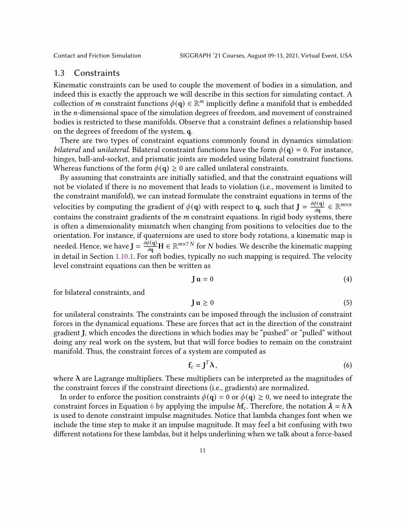
1.3 ConstraintsKinematic constraints can be used to couple the movement of bodies in a simulation, andindeed this is exactly the approach we will describe in this section for simulating contact. Acollection of𝑚 constraint functions 𝜙 (q) ∈ R𝑚 implicitly define a manifold that is embeddedin the 𝑛-dimensional space of the simulation degrees of freedom, and movement of constrainedbodies is restricted to these manifolds. Observe that a constraint defines a relationship basedon the degrees of freedom of the system, q.There are two types of constraint equations commonly found in dynamics simulation:
bilateral and unilateral. Bilateral constraint functions have the form 𝜙 (q) = 0. For instance,hinges, ball-and-socket, and prismatic joints are modeled using bilateral constraint functions.Whereas functions of the form 𝜙 (q) ≥ 0 are called unilateral constraints.By assuming that constraints are initially satisfied, and that the constraint equations will
not be violated if there is no movement that leads to violation (i.e., movement is limited tothe constraint manifold), we can instead formulate the constraint equations in terms of thevelocities by computing the gradient of 𝜙 (q) with respect to q, such that J = 𝜕𝜙 (q)
𝜕q ∈ R𝑚×𝑛
contains the constraint gradients of the𝑚 constraint equations. In rigid body systems, thereis often a dimensionality mismatch when changing from positions to velocities due to theorientation. For instance, if quaternions are used to store body rotations, a kinematic map isneeded. Hence, we have J = 𝜕𝜙 (q)
𝜕q H ∈ R𝑚×7𝑁 for 𝑁 bodies. We describe the kinematic mappingin detail in Section 1.10.1. For soft bodies, typically no such mapping is required. The velocitylevel constraint equations can then be written as
J u = 0 (4)
for bilateral constraints, andJ u ≥ 0 (5)
for unilateral constraints. The constraints can be imposed through the inclusion of constraintforces in the dynamical equations. These are forces that act in the direction of the constraintgradient J, which encodes the directions in which bodies may be “pushed” or “pulled” withoutdoing any real work on the system, but that will force bodies to remain on the constraintmanifold. Thus, the constraint forces of a system are computed as
f𝑐 = J𝑇λ , (6)
where λ are Lagrange multipliers. These multipliers can be interpreted as the magnitudes ofthe constraint forces if the constraint directions (i.e., gradients) are normalized.In order to enforce the position constraints 𝜙 (q) = 0 or 𝜙 (q) ≥ 0, we need to integrate the
constraint forces in Equation 6 by applying the impulse ℎf𝑐 . Therefore, the notation 𝝀 = ℎ λis used to denote constraint impulse magnitudes. Notice that lambda changes font when weinclude the time step to make it an impulse magnitude. It may feel a bit confusing with twodifferent notations for these lambdas, but it helps underlining when we talk about a force-based
11

SIGGRAPH ’21 Courses, August 09-13, 2021, Virtual Event, USA Andrews and Erleben
or impulse-based quantity, i.e. whether time integration has been done to get to a velocity levelform of our models. In computer graphics, the velocity-based form is dominant, and hence wehope the reader will focus more on the mathematical and algebraic forms used for describingthe different kind of constraints.Revising the equations of motion in Equation 3, we include the constraint impulsemagnitudes
as an implicit term, such that
Mu+ − J𝑇𝝀+ = Mu + ℎf, (7)
where 𝝀+ ∈ R𝑚 is a vector of constraint impulse magnitudes. Note that we have not specifiedwhen J is evaluated, and in this course we will consider it to be explicit and constant throughoutthe time step. And so, while the constraint forces are integrated explicitly, it is only in termsof direction, as the Lagrange multipliers enforce the constraint at the end of the time step,i.e., Ju+. However, there are cases when J it is treated implicitly, and thus requires evaluatingthe gradient of 𝜙 (q + ℎΔu+) and resolving for the constraint forces in an iterative fashion.This may mean performing additional collision detection tests, which can negatively impactperformance.For a moment, let us consider just the bilateral constraints in the simulation. The linear
system combining the equations of motion and the velocity constraint equations can be writtenas [
M −J𝑇J 0
] [u+𝝀+
]=
[Mu + ℎ f
0
]. (8)
We use the first row to solve for u+ and substitute our result into the second row to obtain areduced system that we can use to solve for 𝝀+. This technique is called forming the Schurcomplement of the upper left block in Equation 8 and it results in the reduced linear system[
JM−1 J𝑇]︸ ︷︷ ︸
A
𝝀+ + JM−1(Mu + ℎf)︸ ︷︷ ︸b
= 0 , (9)
which is a commonly used form to solve for the constraint impulses. Once 𝝀+ are known, themotion of the degrees of freedom can be recovered using Equation 7. Note that for rigid bodiesand particle systems using lumped masses, the block diagonal form ofM makes it trivial toinvert, and the resulting matrix A will also be positive semi-definite. Whereas, for implicitlyintegrated elastic systems, they will have sparse damping and stiffness matrix contributionsadded to the mass, leading us to choose solvers for Equation 9 that do not involve inversion ofthe upper left block of Equation 8.In the next section, we consider that contact can be modeled as a unilateral constraint with
some special complementarity conditions on the constraint impulses and the relative velocitiesof bodies.
12

Contact and Friction Simulation SIGGRAPH ’21 Courses, August 09-13, 2021, Virtual Event, USA
𝐱
𝐱
𝜙 0
𝐱
𝐱
𝜙 0
𝐱
𝐱
𝜙 0
resting separation penetration
Fig. 1. Illustration of the three contact states determined by the value of the gap function. Observethat a single function value allows us to classify the state.
1.4 Non-interpenetration Contact ConstraintUnlike bilateral constraints, contact constraints are only active when a collision exists betweentwo bodies in the simulation. The state of this relationship between bodies is representedusing a gap function, 𝜙 , which also happens to be the constraint function. The gap function,measures the distance between two bodies, and a positive value 𝜙 > 0 indicates a separationbetween the bodies (see Figure 1).At locations where the gap is zero or negative, 𝜙 ≤ 0, there is a contact between the bodies.
For smooth objects, their unit surface normals will face in opposite directions at the pointof contact. This defines a contact plane containing the point of contact and having a normalvector that is parallel to one of the surface unit normals. Both the contact point and normaldirection are determined during the collision detection phase. For discretized geometries, suchas triangle meshes, it is more tricky to define the contact plane and we discuss this later inSection 2. For now we can continue using our idealized smooth concept of a contact plane.An impulse with magnitude _�̂� is applied at the contact location in order to keep the bodies
from interpenetrating. The non-interpenetration impulse is applied in a direction that isperpendicular to the contact plane. That is, in the normal direction of the surfaces. This leadsto two considerations when applying contact forces. Either the bodies are not in contact andthere is no contact force, in which case
𝜙 > 0, _�̂� = 0 ,
or the bodies are touching (for instance, there is resting contact) and a non-zero contact forceis applied at the contact location, in which case
𝜙 = 0, _�̂� > 0 .
These two cases are exclusive, and often they are succinctly written as the complementarityconditions of contact as
0 ≤ 𝜙 ⊥ _�̂� ≥ 0 . (10)
13

SIGGRAPH ’21 Courses, August 09-13, 2021, Virtual Event, USA Andrews and Erleben
𝐱
contact𝐱𝐉 𝜆
𝐉 𝜆
𝐱
𝐱
𝜙 0 𝜙 0
Fig. 2. Left: Two bodies 𝑖 and 𝑗 not in contact have a positive gap function 𝜙 > 0. Right: A non-interpenetration constraint is created between two colliding bodies. The gap function is zero, and theconstraint is enforced by an impulse with magnitude _�̂� and the direction of the impulse is determinedby the constraint Jacobian J =
[J𝑖 J𝑗
].
Notice that we have used the complementarity operator “⊥”. If 𝑎 and 𝑏 are two scalars, then0 ≤ 𝑎 ⊥ 𝑏 ≥ 0 is defined to mean that 𝑎 ≥ 0, 𝑏 ≥ 0, and 𝑎 𝑏 = 0. The ⊥ notation is a shorthand version that means the same thing.The Equation 10 is termed the position level non-penetration complementarity condition.
Observe that this type of condition says nothing about the tangential motion. Hence, objectscan be in sustained touching contact while sliding relative to each other. Non-sliding sustainedcontact state is often referred to as a resting contact.Figure 2 illustrates the gap function before and after collision, which is positive and zero,
respectively. Usually, when the bodies are sufficiently close to touch, a non-interpenetrationconstraint is created between the two bodies in order to keep them from overlapping. Thedirection of the non-interpenetration impulse is determined by the contact plane, and theimpulse J𝑇_+ is applied to both bodies involved in the collision.Although the positions are used by collision detection to determine if two bodies are in
contact, the constraints in Equation 8 are formulated at the velocity-level . Recognizing thatcontact constraints are generated only when 𝜙 = 0, we can reason about conditions on thevelocities of bodies during contact.Recall that with semi-implicit and implicit integration techniques, the velocities at the end
of a time step are used to advance the simulation. Therefore, if two bodies are touching in thecurrent time step, they will not be touching in the subsequent time step if ¤𝜙 > 0. This is becausethe two bodies will separate due to a positive relative velocity at the contact location. In thiscase, there is no need to apply a contact force, and _�̂� = 0. However, if the relative velocityis zero, ¤𝜙 = 0, then a force is needed to prevent the bodies from further interpenetrating,i.e., _�̂� > 0. Therefore, the velocity level non-penetration complementarity condition may beformally stated as
0 ≤ ¤𝜙 ⊥ _�̂� ≥ 0. (11)
14

Contact and Friction Simulation SIGGRAPH ’21 Courses, August 09-13, 2021, Virtual Event, USA
Here, we note that ¤𝜙 is the normal component of the relative velocity between the bodies at aspecific contact point. Hence, we use the notation ¤𝜙 = 𝑣�̂� for the constraint velocities in theremainder of the notes. This means that if there is a separation velocity 𝑣�̂� > 0 in the normaldirection, then there can be no normal contact impulse. On the other hand, if there is a normalcontact impulse such that _�̂� > 0, then there is a resting contact and therefore 𝑣�̂� = 0.Observe that Equation 11 is the result of approximating Equation 10 by substituting the first
order Taylor expansion for the gap function,𝜙+ ≈ 𝜙+ℎ 𝑣�̂� , and applying the knowledge that𝜙 =
0. Changing the expansion point leads to different schemes and can be used to foresee contactas well as correcting drifting error that arise during simulation from computing approximatesolutions or numerical precision. Detecting and adding constraints prior to touching contactwould result in the scheme using the non-penetration complementary condition
0 ≤ (𝜙 + ℎ𝑣�̂�) ⊥ _�̂� ≥ 0 , (12)where 𝜙 > 0 since contact has not yet happened. This is essentially an explicit first orderapproximation of the gap function. This form is popular to avoid tunneling artifacts of objectsas it anticipates future contact points, and this idea is further discussed in Section 2 of thesenotes.
1.4.1 Non-interpenetration Jacobian. Next, let us consider how to compute 𝑣�̂� . We will firstpresent the ideas for the case of rigid bodies and following this we will demonstrate howto work with soft bodies. Noting that 𝑣�̂� is the rate of change of the gap function, ¤𝜙 , and byapplying some straightforward calculus, we get
𝑣�̂� = ¤𝜙 ≡𝜕𝜙
𝜕𝑡=𝜕𝜙
𝜕q𝜕q𝜕𝑡
=𝜕𝜙
𝜕qH︸︷︷︸
J
u = J u . (13)
In the last step, we have used the kinematic relationship for rigid bodies ¤q = Hu fromEquation 1.2. This gives us a mathematical understanding of J. Looking more closely we noticethat the role of the Jacobian matrix is to map body-space velocities into a velocity for the gapfunction. That is, we map from body-space to measure how fast the gap function is changing.Using this insight, J for the non-penetration constraints may be constructed more precisely.
Consider two rigid bodies, 𝐴 and 𝐵, with centre of mass positions x𝐴 and x𝐵 that are collidingat contact point p with unit contact normal �̂� pointing from 𝐴 towards 𝐵. The relative velocityin the normal direction 𝑣�̂� is then given by
𝑣�̂� = �̂� · Δv , (14)where Δv is the relative contact point velocity given by
Δv = (v𝐵 + 𝜔𝐵 × (p − x𝐵)) − (v𝐴 + 𝜔𝐴 × (p − x𝐴)) . (15)Here, v𝐴 and v𝐵 are the linear velocities of center of masses and 𝜔𝐴 and 𝜔𝐵 are the angularvelocities. This notation is illustrated in left side of Figure 3.
15

SIGGRAPH ’21 Courses, August 09-13, 2021, Virtual Event, USA Andrews and Erleben
𝐱
𝐱𝜔
𝐯𝜔
𝐯
𝑛
𝐩𝐫
𝐫
𝐴
𝐵
rigid bodies soft bodies
𝑛
𝐩𝑙
𝑗𝑘
𝑖
𝑚
𝐴𝐵
Fig. 3. Left: the notation involved in computing the relative contact point velocity of two rigid bodiesare depicted. Right: The normal and vector arms and barycentric coordinates are the informationneeded to evaluate the contact Jacobian for two soft bodies modeled by tetrahedral elements.
Using the shorthand r𝐴 = (p − x𝐴) and r𝐵 = (p − x𝐵), the definition of the skew-symmetriccross product matrix of a vector r =
[𝑥 𝑦 𝑧
]𝑇 is
r× ≡
0 −𝑧 𝑦
𝑧 0 −𝑥−𝑦 𝑥 0
. (16)
The relative velocity in the normal direction can then be written as the matrix-vector product
𝑣�̂� =[−�̂�𝑇 �̂�𝑇 r×
𝐴�̂�𝑇 −�̂�𝑇 r×
𝐵
]︸ ︷︷ ︸J
v𝐴𝜔𝐴v𝐵𝜔𝐵
︸︷︷︸u
. (17)
This two-body system may be extended to include more body velocities in the system general-ized velocity vector u and by adding corresponding zero-blocks to J. Extending to multiplecontact points means we get multiple rows in the Jacobian. Each one will have a structuresimilar to Equation 17, but with kinematics that are specific to each contact.
1.4.2 Non-interpenetration Constraint for Soft Bodies. The case of a soft body can be derivedsimilar to the rigid body case. Often, a computational mesh is used to model the surface orvolume of a soft body (e.g., a linear tetrahedral mesh). We will use this as our working examplewithout loss of generality. Imagine a node of soft body 𝐴 touches a face of a tetrahedron fromsoft body 𝐵. Let the position and velocity of the node from body 𝐴 be given by x𝑙,𝐴 and v𝑙,𝐴where 𝑙 is the node index from body 𝐴. Let the four nodes defining the tetrahedron from body𝐵 be given by x𝑖,𝐵 , v𝑖,𝐵 , x 𝑗,𝐵 , v 𝑗,𝐵 , x𝑘,𝐵 , v𝑘,𝐵 , x𝑚,𝐵 , and v𝑚,𝐵 where 𝑖 , 𝑗 , 𝑘 , and𝑚 are the node
16

Contact and Friction Simulation SIGGRAPH ’21 Courses, August 09-13, 2021, Virtual Event, USA
indices in body 𝐵. At the point of contact p we have
p = x𝑙,𝐴 = 𝑤𝑖x𝑖,𝐵 +𝑤 𝑗x 𝑗,𝐵 +𝑤𝑘x𝑘,𝐵 +𝑤𝑚x𝑚,𝐵 , (18)
where𝑤𝑖 ,𝑤 𝑗 ,𝑤𝑘 , and𝑤𝑚 are the barycentric coordinates of p with respect to the tetrahedron.See the right side of Figure 3 for an illustration of the concepts. The relative contact pointvelocity in the contact normal direction is then given by
𝑣�̂� = �̂� ·(𝑤𝑖v𝑖,𝐵 +𝑤 𝑗v 𝑗,𝐵 +𝑤𝑘v𝑘,𝐵 +𝑤𝑚v𝑚,𝐵 − v𝑙,𝐴
), (19)
and this can again be rewritten as a matrix-vector product, such that
𝑣�̂� =[−�̂�𝑇 𝑤𝑖�̂�
𝑇 𝑤 𝑗�̂�𝑇 𝑤𝑘�̂�
𝑇 𝑤𝑚�̂�𝑇]︸ ︷︷ ︸
J
v𝑙,𝐴v𝑖,𝐵v 𝑗,𝐵v𝑘,𝐵v𝑚,𝐵
︸ ︷︷ ︸u
. (20)
Here, only the nodes involved in the contact are include in the Jacobian matrix J and thevector of node velocities u. However, soft bodies usually contain many more nodes that needto be included into the system velocity vector u, and thus corresponding zero blocks shouldbe added to the Jacobian. As with the rigid body case, adding more contact points results inadding more rows of similar pattern to the system Jacobian. One may derive other specificformulas for the Jacobian in cases of contact between two nodes only, or two tetrahedra, orone node from soft body and one rigid body, and so on.
1.5 The Coulomb Friction LawFriction is an important phenomena we must simulate in graphics applications. This introducesadditional constraints on the movement of bodies in the simulations and the forces generatedwithin the plane of contact.In order to describe friction we will define a local contact frame for a single point of contact.
This is called the contact frame and it consist of two orthogonal unit vectors that span thecontact plane, let us call them 𝑡 and 𝑏, the contact plane can be viewed as the shared tangentplane between two smooth surfaces at a point of contact, p. Orthogonal to the contact plane wehave the contact normal direction. One can think of this as the direction where one at myopicscale must prevent motion to avoid penetration, we denote this direction by �̂�. There are twochoices for which the direction of the normal could point in. If the two surfaces in contact arelabelled 𝐴 and 𝐵 then we adopt the convection that the normal points from 𝐴 towards 𝐵, andthat 𝑡 , 𝑏 and �̂� forms a right handed coordinate system. This local coordinate system is used todescribe the contact physics in. The contact frame is illustrated in Figure 4. Sometimes theframe is referred to as the contact basis, contact coordinate system or contact space. Observe
17

SIGGRAPH ’21 Courses, August 09-13, 2021, Virtual Event, USA Andrews and Erleben
𝑛
𝑏�̂�
𝐴
𝐵
contact plane
𝐩
Fig. 4. The contact frame defines a right-handed coordinate system and is defined by the two tangentplane vectors 𝑡 and 𝑏 and the plane normal vector �̂�.
that the normal can be defined from the spatial derivative of the gap function we introducedin Section 1.4. There exist infinite many choices for generating the tangent vectors 𝑡 and 𝑏.When working with isotropic friction model it is from the model viewpoint not important howthese vectors are generated but for anisotropic friction their choice is critical in aligning thefriction cone properly between the two surfaces. We treat this in more detail in Section 4.1.When describing friction forces in the contact space then we need to know the relative
velocity of the surfaces in our contact frame. Let Δv be the relative velocity of the surfaces inworld space. Then, the contact space version is:
v =[�̂� 𝑡 𝑏
]𝑇︸ ︷︷ ︸C𝑇
Δv (21)
Notice that we picked the normal as the first basis vector in this transformation. This is just aconvenient convention when we would like to have the normal part of the contact problemsolved before the tangential components.Realizing that the relative contact point velocity in world space between two rigid bodies is
given by Equation 15, we can now write the contact space velocity as
v = C𝑇[−I3×3 r×
𝐴I3×3 −r×𝐵
]︸ ︷︷ ︸J
v𝐴𝜔𝐴v𝐵𝜔𝐵
︸︷︷︸u
, (22)
where I3×3 is the 3-by-3 identity matrix. We see here that J has simply been extended withthe tangent vectors compared to our previous non-frictional case. The J is called the contactJacobian and from above equation we observe that is role is simply to map body-velocitiesfrom world-space into the contact space velocity. We have now explained how the Jacobian
18

Contact and Friction Simulation SIGGRAPH ’21 Courses, August 09-13, 2021, Virtual Event, USA
from Equation 17 can be extended to include tangential velocities and the same extension cantrivially be done for the soft body Jacobian in Equation 20. In the following we let 𝑣�̂� denotethe normal component of the contact space velocity and v𝑡 the tangential component spannedby 𝑡 and 𝑏, similar notation is used for the contact impulse, where _�̂� ∈ R is the normal impulseand 𝝀𝑡 ∈ R2 is the tangential impulse (i.e., friction force between two surfaces). In this sectionwe present a physical law that describes this force.
1.5.1 Theory of Friction. Coulomb friction couples the normal impulse _�̂� and tangentialimpulses. The exact isotropic planar Coulomb friction cone constraint, for tangential frictionforce 𝝀𝑡 applied to colliding bodies, can be written as
∥𝝀𝑡 ∥2 ≤ `_�̂� . (23)The non-linear inequality in Equation 23 defines a quadratic cone. The coefficient ` is calledthe coefficient of friction and is a unit-less non-negative value that relates friction force to thenormal force. The coefficient of friction is specific in regards to the two types of materials thatare in contact. When setting up simulations one often have to specify its value which can bebound measured data. We added a small table below with common values. The `-coefficient isfrom a practical viewpoint considered to be a material-parameter only. We list some typicalvalues for the coefficient of friction in Table 1
Materials and MaterialCombinations
Surface Conditions Frictional Coefficient
Static Kinetic (sliding)Aluminum - Aluminum Clean and Dry 1.05 - 1.35 1.4Aluminum - Aluminum Lubricated and Greasy 0.3Cast Iron - Cast Iron Clean and Dry 1.1 0.15Car tire - Asphalt Clean and Dry 0.72Car tire - Grass Clean and Dry 0.35Ice - Wood Clean and Dry 0.05Leather - Oak Parallel to grain 0.61 0.52Rubber - Dry Asphalt Clean and Dry 0.9 0.5 - 0.8Steel - Steel Clean and Dry 0.5 - 0.8 0.42Steel - Steel Lubricated and Greasy 0.16Steel - Steel Castor oil 0.15 0.081
Table 1. Coefficients of friction for various pairs of materials (from “The Engineering Toolbox” (https://www.engineeringtoolbox.com/). Observe that the coefficient of friction depends on environmentalchanges.
The Coulombmodel is an empirical model, meaing that it has been derived from observationsfrom measurements. The field of tribology is, among other things, concerned with explaining
19

SIGGRAPH ’21 Courses, August 09-13, 2021, Virtual Event, USA Andrews and Erleben
the physical cause to the friction force. It turns out that friction is a quite complicated matterand many factors influence its behavior, and friction is essentially a system response. Thecauses of friction are explained from theory of asperities. At micro-scale level the asperities aresticking out of the material surfaces and when objects come into contact the asperities deform,break and plow through the surfaces thereby causing "resistance" to motion. It is this resistancethat we humans perceive as the friction force. Besides the micro-scale geometry many otherfactors influence the behavior such as lubrication, electrostatic effects, third-party obstacleslike small grains or dust, humidity and temperature, elastic and plastic micro-deformations ofthe surfaces, tear and wear and many more effects. The coefficient of friction can be understoodas boiling all that complexity down to a single number. This is convenient from a modelingviewpoint as it makes it feasible for us to simulate many objects with complex shapes subject tofrictional contact interaction. The Coulomb model is not perceived as being very accurate, butits simplicity makes it very appealing and thus is has wide-scale adoption for contact simulation.It is generally accepted that the coefficient of friction changes value when a transition fromstatic friction (sticking) to dynamic friction (sliding) happens. It may be explained from bondingof asperities breaking when sliding happens and the dynamic coefficient of friction is thereforelower than that static one. The actual transition from sticking to sliding is called the onset offriction.Let us return to setting up our model of friction that we use in multibody simulations for
rigid and soft bodies in the field of computer graphics. The isotropic Coulomb friction law isin fact a two-part law:• Slip: If the bodies are sliding relative to each other, then the direction of the friction forceis opposed to the tangential relative velocity and its magnitude is `_�̂� .• Stick: If the objects are not moving relative to each other, then the friction force can haveany direction as long as the inequality in Equation 23 holds.
We can express both cases mathematically as follows
` · _�̂� −√︁𝝀𝑡 · 𝝀𝑡 ≥ 0 , (24a)
∥v𝑡 ∥(`_�̂� −
√︁𝝀𝑡 · 𝝀𝑡
)= 0 , (24b)
∥v𝑡 ∥∥𝝀𝑡 ∥ = −v𝑡 · 𝝀𝑡 . (24c)
Observe here how the term ∥v𝑡 ∥ act as a switch for selecting between the cases of slipping orsticking. If ∥v𝑡 ∥ = 0 then the last two conditions are trivially fulfilled and the first conditionessentially only tells us that the friction force must belong to the friction cone. On the otherhand, if ∥v𝑡 ∥ > 0 then the two last conditions kick in. The first one ensures the frictionforce is maximized, and the last one ensures that the friction force is opposing the slidingdirection. This is illustrated in Figure 5. This form of the isotropic Coulomb friction model isfrequently used for modeling frictional contact, and it represents a non-linear complementarityproblem (NCP) formulation of frictional contact. However, in Section 1.6 and Section 1.7,
20

Contact and Friction Simulation SIGGRAPH ’21 Courses, August 09-13, 2021, Virtual Event, USA
normal
contactplane
friction cone
�̂� 𝑏
1 𝜇
𝛌
𝐯 0
𝑛
normalfriction cone
�̂� 𝑏𝛌
𝐯 0
𝑛
�̂�
𝑏
𝐯 0
𝛌𝜇𝜆�̂�
𝑏
𝐯 0
𝛌
contactplane
Fig. 5. Graphical illustration of the isotropic Coulomb law. Left: the case of slipping is depicted with aunique solution. Right: the case of sticking is shown to have multiple solutions. The bottom row showsthe cone as seen from the top. Observe how the circular shape of the cone makes it particular easy tocompute the friction force.
we present details on how to linearize the Coulomb friction model into the standard linearcomplementarity problem (LCP) and Boxed-LCP forms, which are the origin for the many LCPnumerical methods we cover in Section 3.The stick-slip conditions can be written up in a more general form as they are related to
energy dissipation. If one assumes that the friction force maximally dissipates energy, then inthe case of an isotropic circular friction cone this principle of maximum dissipation reduces tothe stick-slip conditions we introduced above. For the more general force, we start by writingup the definition of the friction cone using a set notation:
F (`_�̂�) ≡{𝛾 ∈ R2 �� ∥𝛾 ∥2 ≤ `_�̂�} . (25)
This set denotes all feasible friction forces for the case of isotropic planar Coulomb friction.One can define the friction cone differently all dependent on the type of materials. For instance,an elliptical shaped cone can be used to model anisotropic friction. The principle of maximumdissipation can now be written as a minimization problem,
𝝀𝑡 = arg min𝛾∈F (`_�̂�)
v𝑡 · 𝛾 . (26)
21

SIGGRAPH ’21 Courses, August 09-13, 2021, Virtual Event, USA Andrews and Erleben
That is to say the friction force is given by the force that instantaneously removes most (i.e.maximum dissipation) energy from the system.If the friction cone F is a strict convex set then the minimization problem has an unique
solution that are characterized by the first order necessary optimality conditions. If wemomentarily denote the objective function as 𝑓 (𝛾) ≡ v𝑡 · 𝛾 and the convex set as Ω = F (`_�̂�)then these conditions can be written as
− ∇𝛾 𝑓 (_𝑡 ) ∈ NΩ (𝝀 t̂) (27)
where NΩ (𝝀 t̂) is the normal cone of F (`_�̂�) at the position 𝝀𝑡 . The normal cone of a convexset can be defined as follows,
NΩ (𝝀 t̂) ≡{z�� z · (𝛾 − 𝝀 t̂
)≤ 0, ∀𝛾 ∈ Ω
}. (28)
If the set Ω is strictly convex, then we haveNΩ (𝝀𝑡 ) ≡ −v𝑡 . If the set Ω is only convex, then thenormal cone may be a multi-set. This first order optimality condition can be written conciselyas the condition
∀𝛾 ∈ F (`_�̂�) and (𝛾 − 𝝀𝑡 ) · v𝑡 ≥ 0 . (29)
This form is known as a variational inequality (VI) and is often the mathematical formof principle of maximum dissipation that is used as starting point for deriving nonlinearcomplementarity problem (NCP) formulations of the frictional contact problem. These NCPproblems can be solved quite nicely with Newton type of methods. The VI-form given abovecan be used more directly in a numerical method without needing to do the linearizationswe cover below in Sections 1.6 and 1.7. It offer one with a trade-of between a more "difficult"to solve nonlinear problem or an "easier" to solve linear version. The nonlinear form is morecompact than the linear form in the sense that much fewer variables are needed. Due to itscapability to inherently express the non-linearity the VI-form generalizes easily to an-isotropicfriction and proximal operators allow for quite general shaped convex cones.Above we have covered the most typical and classical models for planar dry friction. There
exist other friction models. The above models can be extended trivially to include torsional(Coulomb–Contensou friction) and rolling friction by incorporating angular counter parts, weshow this for torsional friction when we introduce proximal operators in Section 4.1. Thereare many more models as described by Sheng Chen and Liu [2016]. Like the Tresca frictionwhich limits the friction force to a constant magnitude or the Stribek friction model whichis dependent on the velocity magnitude to model effects of lubrication. Some models seekinspiration in micro-scale geometry interaction such as the bristle friction model. In Section 4.2we present a new friction model that has originated in the graphics field that take a micro-scalemodeling approach to present more interesting friction phenomena that go beyond the typicalisotropic Coulomb friction model.
22

Contact and Friction Simulation SIGGRAPH ’21 Courses, August 09-13, 2021, Virtual Event, USA
normal
tangent
friction cone
𝑛
�̂� �̂�
�̂� �̂�
Fig. 6. A friction cone approximated by normal direction �̂� and four friction directions {𝑡1, 𝑡2, 𝑡3, 𝑡4}that are tangent to the contact plane.
1.6 The Linear Complementarity Problem Model of Frictional ContactA linear friction model is preferred for many applications due to their efficiency and compati-bility with a wide variety of numerical solvers. Hence a linearized approximation of the frictioncone introduced in the previous section is often used. Stewart and Trinkle, Anitescu and Potra,among others, linearize the 3D friction model using a polyhedral cone [Anitescu and Potra1997; Stewart and Trinkle 1996]. The polyhedral cone is given by a span of 𝑘 + 1 unit vectors{�̂�, 𝑡1, . . . , 𝑡𝑘}, where �̂� is the normal direction of the contact plane and {𝑡1, . . . , 𝑡𝑘} all lie inthe contact plane (see Figure 6). We use a positive span for the tangent vectors {𝑡1, . . . , 𝑡𝑘},which means that each tangent vector has a twin vector that is oriented in the exact oppositedirection. For instance, notice in Figure 6 that 𝑡2 is opposite 𝑡1. The advantage of using tangentvectors that point in opposite directions is that it allows the friction force to be written withall non-negative numbers in this basis. The disadvantage, from a computational viewpoint, isthat one needs more numbers.One advantage of the non-negative numbers is that they help us couple the sliding direction
to the friction force direction. Let us just show a 1D example to make this modeling trick moreclear. Assume we have some friction force measure 𝑐 along the axis 𝑡 . We can express thismeasure instead using two numbers 𝑎 ≥ 0 and 𝑏 ≥ 0, such that
𝑐 𝑡 = 𝑎 𝑡 − 𝑏 𝑡 . (30)
Notice that 𝑐 can be both a positive and negative number depending on the friction forcedirection and that 𝑐 is now replaced by two non-negative numbers 𝑎 and 𝑏. In the above
23

SIGGRAPH ’21 Courses, August 09-13, 2021, Virtual Event, USA Andrews and Erleben
𝑘 4 𝑘 6 𝑘 8
Fig. 7. The accuracy of the polyhedral cone approximation – light blue shading – increases as thenumber of tangential directions increases. The improvement in accuracy is at the cost of an increasingproblem size.
example, the positive span is made of the two vectors {𝑡,−𝑡}. Observe also that we must have
0 ≤ 𝑎 ⊥ 𝑏 ≥ 0 . (31)
From this it is obvious that 𝑎 is the positive part of 𝑐 and 𝑏 is the negative part of 𝑐 , and as 𝑐can not be both positive and negative at the same time then 𝑎 and 𝑏 must be complementary.The positive span approximation allows us to rewrite Equation 23 as
0 ≤(` _�̂� −
∑︁𝑖
_𝑡𝑖
), (32)
where 𝝀𝑡 =[_𝑡1 · · · _𝑡𝑘
]𝑇 is a vector of friction impulses along the tangent directions. Inthis way, the nonlinear Euclidean norm from the Coulomb model is replaced with the linearform in Equation 32. In principle, one can add as many tangent directions as wanted to get abetter approximation to the exact cone as illustrated in Figure 7.One challenge with this model is to correctly formulate the stick-slip transitions. We have
introduced 𝑘 possible directions for measuring a slipping velocity and we need just one scalarvalue– the slack variable– to determine the correct stick-slip behavior. The idea here is that wedo not need to measure the exact slipping velocity. We only need information about whetherthere is slipping or not. Hence, one idea is to simply to identify the direction of maximumslipping velocity. If we let the maximum slipping velocity along any direction by denoted by𝛽 ≥ 0 then we must have
0 ≤ (𝛽 e + v𝑡 ) (33)where v𝑡 =
[𝑣𝑡1 . . . 𝑣𝑡𝑘
]is the sliding velocity measured along each tangent vector and
where e is a 𝑘 dimensional vector of ones. Observe here that 𝛽 can only be zero if v𝑡 is zero. If𝛽 is positive, then it will have the same value of the maximum component of v𝑡 . Hence, wesay 𝛽 is a estimate or measure of the maximum sliding velocity along the directions of thepositive span of tangent vectors.
24

Contact and Friction Simulation SIGGRAPH ’21 Courses, August 09-13, 2021, Virtual Event, USA
The next step to realize is the condition that if there is slipping the the friction force musthave its maximum value in the opposite direction according to the principle of maximumdissipation. This translates into saying that the friction force should work such that it removesthe maximum amount of energy from the system. To ensure this we will make sure that when𝛽 > 0 then
(` _�̂� −
∑𝑖 _𝑡𝑖
)becomes zero. This means the friction force will have its maximum
allowed value when sliding. However, to get the direction of the friction correct we will force(𝛽 e + v𝑡 ) to become zero when we have a friction component. This means when 𝝀𝑡 > 0 then(𝛽 e + v𝑡 ) = 0.Historically, the variable 𝛽 for switching between the slip and stick regimes is called a “slack”
variable. This name may appear non-intuitive at first, but consider it a measure of the amountof sliding that is present during the current state. It is these stick-slip transitions that makethe frictional problem difficult, and hence why specialized numerical solvers are required todeal with complementarity conditions (as we will see in Section 3).We may now summarize the four ingredients that went into stating a linear model for
isotropic Coulomb friction:
• The non-peneration constraints that turn on and off whether we have sustained contactor separation.• Linearization of the friction cone to remove the non-linear terms.• Replace the measure of slipping velocity with the measure of maximum direction ofslipping velocity, to give us a single switching variable to model stick-slip transitions.• Using the principle of maximum dissipation to pick a unique friction direction whenslipping occurs.
Finally, we can write up the complete mathematical model for our derivation. Letting 𝝀𝑡 =[_𝑡1 · · · _𝑡𝑘
]𝑇 be a vector of friction impulses, the linearized model, including complemen-tarity conditions, can be formally stated as
0 ≤ 𝑣�̂� ⊥ _𝑛 ≥ 0, (34a)0 ≤ (𝛽 e + v𝑡 ) ⊥ 𝝀𝑡 ≥ 0, (34b)
0 ≤(`_�̂� −
∑︁𝑖
_𝑡𝑖
)⊥ 𝛽 ≥ 0. (34c)
The first complementarity constraint in Equation 34 models the non-penetration constraintas before. The second equation makes sure that in case we do have friction _𝑡𝑖 > 0 for some𝑖 , then 𝛽 will estimate the maximum sliding velocity along the 𝑡𝑖 ’s directions. Observe thatEquation 34b is a 𝑘-dimensional vector equation whose main purpose is to choose the direction𝑡𝑖 that is best for the direction of maximum dissipation. The last equation makes sure thefriction force is bounded by the Coulomb friction cone. Notice that if 𝛽 > 0, the last equationwill force the friction force to lie on the boundary of the polyhedral friction cone. If 𝛽 = 0,
25

SIGGRAPH ’21 Courses, August 09-13, 2021, Virtual Event, USA Andrews and Erleben
normal
tangent
friction cone
λ
λ
λ
λ
λ
�̂� �̂�
Fig. 8. The friction cone approximated by a box, where the limits of friction impulses in each tangentialdirection t𝑖 are determined by the box limit equation _𝑙𝑜𝑡𝑖 ≤ _𝑡𝑖 ≤ _
ℎ𝑖𝑡𝑖.
then the two last equations model static friction. That is, no sliding can occur and any frictionforce inside the friction cone is feasible.For a general system consisting of 𝑝 contacts, we can assemble the global Jacobian matrices
containing the non-interpenetration and tangential frictional constraints for all contacts. Thenon-interpenetration Jacobian has a similar form to Equation 22, but with a single row percontact. For example, the 𝑖th contact with normal �̂�𝑖 is
J�̂�,𝑖 =[−�̂�𝑇𝑖 �̂�𝑇𝑖 r
×𝑖,𝐴
�̂�𝑇𝑖 −�̂�𝑇𝑖 r×𝑖,𝐵], (35)
and for all 𝑝 contacts we have J�̂� =[J𝑇�̂�,1 . . . J𝑇
�̂�,𝑝
]𝑇. Here the Jacobian is shown in its concise
form, but in practice care must be taken so that the dimensions of the global matrix match thedegrees of freedom of the dynamical system.The frictional Jacobian is assembled in a similar way, but with 𝑘 rows per that correspond to
the friction basis in Figure 7, such that for contact 𝑖 the matrix is
J𝑡,𝑖 =
−𝑡𝑇𝑖,1 𝑡𝑇𝑖,1r
×𝑖,𝐴
𝑡𝑇𝑖,1 −𝑡𝑇𝑖,1r×𝑖,𝐵...
......
...
−𝑡𝑇𝑖,𝑘
𝑡𝑇𝑖,𝑘r×𝑖,𝐴
𝑡𝑇𝑖,𝑘−𝑡𝑇𝑖,𝑘r×𝑖,𝐵
, (36)
26

Contact and Friction Simulation SIGGRAPH ’21 Courses, August 09-13, 2021, Virtual Event, USA
and for all 𝑝 contacts we have J𝑡 =
[J𝑇𝑡,1 . . . J𝑇
𝑡,𝑝
]𝑇. Finally, the constrained equations of
motion for the system (i.e., in the form of Equation 8) may be written asM −J𝑇
�̂�−J𝑇
𝑡0
J�̂� 0 0 0J𝑡 0 0 E0 �̄� −E𝑇 0
u+𝝀+�̂�
𝝀+𝑡
𝛽
+−Mu − ℎf
000
=
0v�̂�v𝑡0
(37a)
0 ≤ v�̂� ⊥ 𝝀+�̂� ≥ 0 (37b)0 ≤ (v𝑡 + E𝛽) ⊥ 𝝀+
𝑡≥ 0 (37c)
0 ≤ �̄�𝝀+�̂� − E𝑇𝝀+
𝑡⊥ 𝛽 ≥ 0 (37d)
where �̄� = diag( [`1 . . . `𝑝
] )is a diagonal matrix containing friction coefficients of each
contact, and E = diag( [e𝑇1 . . . e𝑇𝑝
] )is a block diagonal matrix containing 𝑘 dimensional
vectors of ones. By applying the Schur complement “trick” here, we can compute the reducedsystem (
C + GM−1G𝑇)
︸ ︷︷ ︸A
𝝀+�̂�
𝝀+𝑡
𝛽
︸︷︷︸x
+GM−1 (Mu + ℎf)︸ ︷︷ ︸b
=
v�̂�v𝑡0
, (38)
where
C =
0 0 00 0 E�̄� −E𝑇 0
, and G𝑇 =[J𝑇𝑡
J𝑇�̂�
0].
Then, Equation 37a can be written concisely and compactly in the form of a standard LCPform as
0 ≤ Ax + b ⊥ x ≥ 0 . (39)
This illustrates how powerful the LCP model really is. By simply assembling the A matrix andb vector, we can call our favorite LCP solver to compute x. The system may be slightly reducedby noting that the first row in the system can be used to eliminate u+. This rewrite is similarto how Equation 8 was transformed in Equation 9 using the Schur complement. Anotherimportant observation here is that A is asymmetric for the LCP model. This has consequenceswith regards to the solvers than can be applied to this model. However, the boxed model wederive in the next section breaks the coupling of the tangent directions and this leads to amatrix A that is symmetric. .
27

SIGGRAPH ’21 Courses, August 09-13, 2021, Virtual Event, USA Andrews and Erleben
1.7 The Boxed Linear Complementarity Problem Model of FrictionalContact
An alternative for discretizing the friction cone can be seen in Figure 8. Using two orthogonaltangent directions, one can write independent inequalities in each friction direction to havethe sliding force limited by the coefficient of friction, `, times the normal force, _�̂� . That is,
_lo𝑡1≤ _𝑡𝑖 ≤ _
hi𝑡1
(40a)
_lo𝑡2≤ _𝑡2 ≤ _
hi𝑡2
(40b)
where _𝑙𝑜𝑡𝑖= −`_�̂� and _ℎ𝑖𝑡𝑖 = `_�̂� . Some iterative solvers update these friction bounds during the
solve based on the magnitude of the normal forces, yielding a four-sided pyramidal cone that islarger than the true friction cone (in contrast to the approximation in Figure 6 which is insidethe true cone). A further approximation is made by other solvers: using a preliminary solve ofthe normal forces, the bounds can be set and the system can be solved with box friction limits.The bounds on friction impulses in Equations 40a-40b requires us to develop a numerical
method for a problem class which is slightly more general than the classic LCP. Problems inthis more general class are called boxed linear complementarity problems (BLCP).One appealing notational benefit of writing the contact and friction models as a BLCP is
that both the non-penetration constraints and friction bounds can be expressed with the samealgebraic notation simply by changing how the lower and upper bounds are defined. Forinstance, normal impulses have lower and upper bounds _lo
�̂�= 0 and _hi
�̂�= ∞. We demonstrate
this by allowing the index 𝑖 to refer to a friction variable or a normal impulse, and then makeappropriate changes to the bounds. Given _𝑖, 𝑣𝑖, _lo𝑖 , _
hi𝑖 ∈ R, the following three conditions
must be satisfied:
𝑣𝑖 > 0⇒ _𝑖 = _lo𝑖 (41a)
𝑣𝑖 < 0⇒ _𝑖 = _hi𝑖 (41b)
𝑣𝑖 = 0⇒ _lo𝑖 ≤ _𝑖 ≤ _hi𝑖 (41c)
The variables _lo𝑖 and _hi𝑖 are the lower and upper bounds on _𝑖 , and usually it is assumed that_lo𝑖 < _hi𝑖 . We note that by decomposing the residual velocity as 𝑣𝑖 = +𝑣−−𝑣𝑖 , the BLCP can bewritten as three separate LCPs:
0 ≤ +𝑣𝑖 ⊥ (_𝑖 − _lo𝑖 ) ≥ 0 (42a)
0 ≤ −𝑣𝑖 ⊥ (_hi𝑖 − _𝑖) ≥ 0 (42b)0 ≤ −𝑣𝑖 ⊥ +𝑣𝑖 ≥ 0 (42c)
Similar to the polyhedral cone version of the LCP from Section 1.6, a linear system for 𝑝contacts can be assembled. We begin with the Jacobian matrix for a single contact 𝑖 , which is
28

Contact and Friction Simulation SIGGRAPH ’21 Courses, August 09-13, 2021, Virtual Event, USA
given by
J𝑖 =−�̂�𝑇𝑖 �̂�𝑇𝑖 r
×𝑖,𝐴
�̂�𝑇𝑖 −�̂�𝑇𝑖 r×𝑖,𝐵−𝑡𝑇𝑖,1 𝑡𝑇𝑖,1r
×𝑖,𝐴
𝑡𝑇𝑖,1 −𝑡𝑇𝑖,1r×𝑖,𝐵−𝑡𝑇𝑖,2 𝑡𝑇𝑖,2r
×𝑖,𝐴
𝑡𝑇𝑖,2 −𝑡𝑇𝑖,2r×𝑖,𝐵
. (43)
This is in fact the same Jacobian matrix from Equation 22, where 𝑡1 = 𝑡 and 𝑡2 = 𝑏. The globalJacobian matrix can then be written as J =
[J𝑇1 . . . J𝑇𝑝 ∈ R3𝑝×𝑛]𝑇 . Finally, we write global
BLCP of the constrained equations of motion as:[M −J𝑇J 0
]︸ ︷︷ ︸
A
[u+𝝀+
]+
[−Mu − ℎf
0
]︸ ︷︷ ︸
b
=
[0v
], (44a)
0 ≤ +v ⊥ 𝝀+ − 𝝀lo ≥ 0 , (44b)
0 ≤ −v ⊥ 𝝀hi − 𝝀+ ≥ 0 , (44c)0 ≤ −v ⊥ +v ≥ 0 . (44d)
Note that in the above formulation, the constraint impulses are ordered according to the rows ofJ, such that 𝝀+ =
[_�̂�1 _𝑡1,1 _𝑡1,2 . . . _�̂�𝑝 _𝑡𝑝,1 _𝑡𝑝,2
]𝑇 . The Schur complement may be usedto eliminate the variable u+ from this system, similar to how Equation 8 was transformed inEquation 9, and we need only solve for 𝝀+. From top row we obtain u+ = M−1J𝑇𝝀+ + u+ℎM−1fand substitution into the bottom row yields
JM−1J𝑇︸ ︷︷ ︸A
𝝀+ +(−Ju − ℎJM−1f
)︸ ︷︷ ︸b
= v , (45a)
0 ≤ +v ⊥ 𝝀+ − 𝝀lo ≥ 0 , (45b)
0 ≤ −v ⊥ 𝝀hi − 𝝀+ ≥ 0 , (45c)0 ≤ −v ⊥ +v ≥ 0 . (45d)
1.8 The Cone Complementarity Problem for Frictional ContactThe Coulomb friction model we introduced in Section 1.5 combined with the non-penetrationconstraint from Section 1.4 is essentially a nonlinear combinatorial problem. It is by its verynature really not an optimization problem. In this section we will introduce a relaxationtechnique that changes the original model but in such a way that we obtain a convex mini-mization problem. We will start our rewrite of the contact force model by changing the normalnon-penetration constraint to the form [Anitescu and Hart 2004]
0 ≤ 1ℎ𝜙 + 𝑣�̂� − `
√︃𝑣2𝑡+ 𝑣2
𝑏⊥ _𝑛 ≥ 0 . (46)
29

SIGGRAPH ’21 Courses, August 09-13, 2021, Virtual Event, USA Andrews and Erleben
Here v = {𝑣�̂�, 𝑣𝑡 , 𝑣𝑏} is the contact space velocity. Usually we have 𝜙 = 0 for touching contactsand then the equation simplifies to
0 ≤ 𝑣�̂� − `√︃𝑣2𝑡+ 𝑣2
𝑏⊥ _�̂� ≥ 0 . (47)
This is essentially the only change we are making, everything else we keep the same. Whatremains is a bit of mathematical convenience in rewriting everything into a simple form. Wewill now combine this relaxed normal non-penetration constraint with the isotropic planarCoulomb model from previously. This time we will write up both the normal and friction partssimultaneously into one single equation. To do so we need to recall a few definitions frommath. The dual cone to a convex cone K is defined as
K★ ≡ {y | y · x ≥ 0,∀x ∈ K} . (48)The polar cone to a convex cone K is defined as
K◦ ≡ {y | y · x ≤ 0,∀x ∈ K} . (49)Observe we have K◦ = −K★. We now have enough cone-formalism to proceed with puttingour model together. Recall that the isotropic Coulomb friction law stated that `_�̂� ≥
𝝀 t̂ ,
where 𝝀𝑡 = (_𝑡 , _𝑏)𝑇 . This we can rewrite into `2_�̂� − _2
𝑡− _2
𝑏≥ 0. Now let us define the convex
friction cone as follows,
F` ≡{𝝀 = (_�̂�, _𝑡 , _𝑏)
𝑇 ∈ R3��� √︃_2
𝑡+ _2
𝑏≤ `_�̂�
}. (50)
This is a little different from the previous meaning of F (`_�̂�) where _�̂� was seen as an inputparameter that generates a specific cone. The new notation allow us to write _ ∈ F` to expressthe bound of the Coulomb friction law. We now write the combined normal and frictionconstraints simply as a cone complementarity problem (CCP),
F★` ∋ v ⊥ _ ∈ F` , (51)
or equivalently,F ◦` ∋ −v ⊥ _ ∈ F` . (52)
The cone complementary notation means that− v ∈ F ◦` , 𝝀 ∈ F` , and − v · 𝝀 = 0 . (53)
For the isotropic Coulomb friction cone we see that the dual cone is defined as
F ◦` ≡{v = {𝑣�̂�, 𝑣𝑡 , 𝑣𝑏} ∈ R
3��� √︃𝑣2
𝑡+ 𝑣2
𝑏≤ 1
`𝑣�̂�
}. (54)
Figure 9 illustrates the difference between the nonlinear complementarity problem (NCP)formulation of the friction contact we have presented previously and the new cone comple-mentarity problem (CCP) model we just presented.As the figure illustrates the CCP model can be written quite compact and that the sliding
velocity v has been relaxed. That is we have given it more “freedom” not to be confined to the
30

Contact and Friction Simulation SIGGRAPH ’21 Courses, August 09-13, 2021, Virtual Event, USA
𝛌∗
𝐯
𝛌∗
𝐯
ℱ
ℱ∘
ℱ
Fig. 9. On the left the solution from the classical complementary problem formulation is shown. Herethe sliding velocity is confined to be in the 2D contact place. On the right the cone-complementarityformulation (CCP) is shown. Observe in CCP that sliding velocity is now orthogonal to the contactforce.
2D contact plane. Furthermore, the polar cone keeps the velocity orthogonal to the contactforce. Combined those traits give this model many numerical benefits in terms of havingvery fast iterative solvers with sub-linear convergence rates. Projected gradients methods wasinitially explored and are similar in spirit to the project Gauss-Seidel methods we cover in thiswork [Anitescu and Tasora 2010]. The accelerated projected gradient descent method (APGD)is another such method with convergence rate O
(1𝑘2
)where 𝑘 is the iteration number [Mazhar
et al. 2015]. In comparison to the proximal operator methods we present in Section 4.1 for theNCP type of model they have O
( 1𝑘
). A modified Fischer-Burmeister function can be used to
rewrite the CCP model into a root search problem and by applying a splitting strategy onemay develop Gauss-Seidel type solvers from this setting too [Daviet et al. 2011].Hence, there are obvious performance benefits from this formulation of the contact forces.
The catch is that the “physics” is different from the classical model. As Figure 9 clearly shows,as the tangential sliding velocity grows large the model will gain a positive normal componentbased on the relative contact velocity, 𝑣�̂� > 0. In other words, if one has a stack of blocks andpushes a block very fast, then it will try to lift of from the other blocks. The effect can belimited with adding an adhesion term to the model, but it does not completely remove theeffect and adhesion will also further change the physical behavior.Whether the physics of the NCP versus the CCP model is right or wrong is debatable as
friction is a system response and surface material interactions are therefore quite a complicatedmatter to model and there is huge variation. The CCP are disliked by some as it feels likea mathematical rewrite to the physics to get nice numerical properties, and it is loved byothers because the numerical traits the CCP model gains results in very fast solvers. Work hasbeen done on validating the CCP model in context of granular flows and here it shows goodagreement with reality [Mazhar et al. 2015].
31

SIGGRAPH ’21 Courses, August 09-13, 2021, Virtual Event, USA Andrews and Erleben
Recalling the Schur complement reduction technique we used to derive the reduced form inEquation 9, then from
v = Ju+ , (55a)
Mu+ = J𝑇𝝀 +Mu + ℎf (55b)
one can derive the linear relationship between sliding velocity and contact forces as
v = A𝝀 + b . (56)
Substituting this equation into the CCP model, we observe that the model is equivalent to thefirst order optimality conditions of a second order cone problem (SOCP), which is given by
𝝀∗ ≡ arg min𝝀∈F`
12𝝀
𝑇A𝝀 + 𝝀𝑇b . (57)
Notice here that both the objective function and the constraints are written as convex secondorder cones. This insight opens up for the application of a vast majority of numerical methodsfor solving the CCPmodel, such as alternating directionmethod of multipliers (ADMM) [Tasoraet al. 2021]. One may alternatively have used the Schur complement to reduce to a quadraticobjective function in v instead of 𝝀 as was done in [Acary et al. 2011]. The ADMM methodmay be used on this alternative velocity form of the CCP model too [Daviet 2020].We do not cover solvers for CCP frictional contact models in these notes. However, with the
material presented later on iterative methods for NCPs, LCPs, BLCPs and proximal operators,the reader should be off to a good start to implement numerical methods for CCP type modelstoo.
1.9 Constraint StabilizationThe system in Equation 8, and its reduced form in Equation 9, are linear approximationsof a non-linear dynamical systems. Therefore, they are prone to numerical drift, especiallywhen combined with the low-order numerical integration methods that are commonplacein computer graphics applications. Also, an exact numerical solution of the linear systemis practically impossible, which again contributes to the drift. In the context of contactsimulation, this results in both position and velocity level artifacts. At the position level,the interpenetration between bodies will increase since non-interpenetration constraintscannot be exactly resolved, whereas at the velocity level, bodies will begin to slide rather thanstick. Furthermore, if discrete collision detection is used to generate contact constraints, thismeans that collision events may not be detected at the time of impact and hence we cannotassume that bodies will be in a non-interpenetrating state at the start of a time step.The issues described above will cause a multibody system to gradually violate the constraint
manifold. Recall that the manifold is an invariant set defined by the gap function, where𝜙 (q) ≥ 0. An approach to solve this problem would be to use a feedback rule to bring thesystem back to a valid state, where the constraints are not violated. Giving some physical
32

Contact and Friction Simulation SIGGRAPH ’21 Courses, August 09-13, 2021, Virtual Event, USA
meaning to this idea, a spring in the constraint space may be used to “push” or “pull” themultibody system back to the constraint manifold. If there is no constraint violation, thenthis constraint spring generates no forces. However, if there is a constraint violation (e.g.,𝜙 (q) < 0), then the spring generates a force to restore the configuration back to the constraintmanifold. Essentially, the spring force stabilizes the constraint.To realize this behavior, let us assume that all constraint forces are generated by an implicit
Hookean spring, such thatλ+ = −𝑘𝜙+ − 𝑏𝑣+ . (58)
Here, 𝜙 is the gap function, 𝑣 is the relative velocity in constraint space, and 𝑘 and 𝑏 are thestiffness and damping coefficients of the spring. Note that we again adopt the convention that□+ is an implicit variable.Equation 58 is in fact an example of the well known Baumgarte stabilization [Baumgarte
1972] technique. Approximating the constraint error term by 𝜙+ = 𝜙 +ℎ𝑣+, the spring equationcan be rewritten as
λ+ + (ℎ𝑘 + 𝑏) 𝑣+ = −𝑘𝜙,which is further simplified by dividing both sides by (ℎ𝑘 + 𝑏), such that
𝑣+ + 1ℎ𝑘 + 𝑏λ
+ = − 𝑘
ℎ𝑘 + 𝑏𝜙.
Finally, recall that 𝑣+ = Ju+, and further simplification of the above equation yields:
Ju+ +(
1ℎ2𝑘 + ℎ𝑏
)︸ ︷︷ ︸
𝜖
𝝀+ =
(ℎ𝑘
ℎ𝑘 + 𝑏
)︸ ︷︷ ︸
𝜐
−𝜙ℎ. (59)
Note that Equation 59 resembles Equation 4, but introduces a feedback term on the right-handside of the equation. This term attempts to reduce the constraint violation 𝜙 by applying aconstraint-space spring impulse in order to resolve the error by end of the time step. However,the portion of the constraint error being reduced at each step is modulated according to𝜐, which is commonly known as the error reduction parameter (ERP). Observe that setting𝜐 = 1 will encourage the feedback rule to produce a constraint velocity that reduces all of theconstraint error in a single step. Also, observe that a portion of the implicit constraint force _+is now being mixed with the kinematic constraint in Equation 59, and it is often referred to asthe constraint force mixing (CFM) term.The 𝜖 and 𝜐 parameters may be specified directly, which is intuitive from a numerical
standpoint. Whereas adjusting 𝑘 and 𝑏 and then generating 𝜖 and 𝜐 from the spring coefficientsis perhaps amore physically intuitive approach, since there is some notion that these behave likematerial properties of the contact. Additionally, parameters 𝑘 and 𝑏 may be tuned independentof the time step ℎ.
33
SIGGRAPH ’21 Courses, August 09-13, 2021, Virtual Event, USA Andrews and Erleben
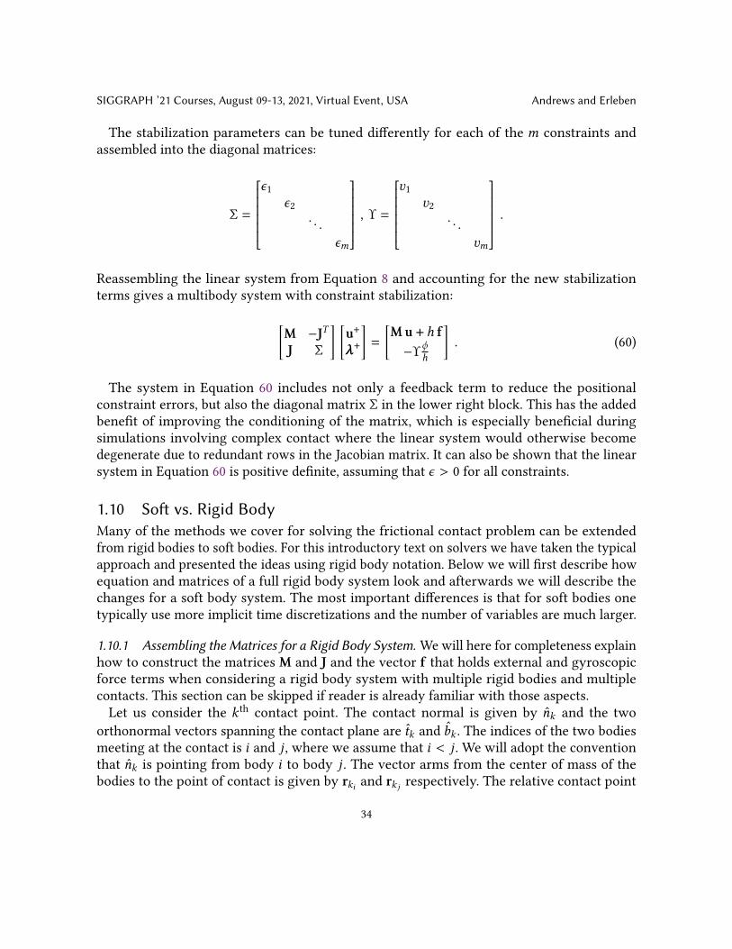
The stabilization parameters can be tuned differently for each of the 𝑚 constraints andassembled into the diagonal matrices:
Σ =
𝜖1
𝜖2. . .
𝜖𝑚
, Υ =
𝜐1
𝜐2. . .
𝜐𝑚
.Reassembling the linear system from Equation 8 and accounting for the new stabilizationterms gives a multibody system with constraint stabilization:[
M −J𝑇J Σ
] [u+𝝀+
]=
[Mu + ℎ f−Υ𝜙
ℎ
]. (60)
The system in Equation 60 includes not only a feedback term to reduce the positionalconstraint errors, but also the diagonal matrix Σ in the lower right block. This has the addedbenefit of improving the conditioning of the matrix, which is especially beneficial duringsimulations involving complex contact where the linear system would otherwise becomedegenerate due to redundant rows in the Jacobian matrix. It can also be shown that the linearsystem in Equation 60 is positive definite, assuming that 𝜖 > 0 for all constraints.
1.10 Soft vs. Rigid BodyMany of the methods we cover for solving the frictional contact problem can be extendedfrom rigid bodies to soft bodies. For this introductory text on solvers we have taken the typicalapproach and presented the ideas using rigid body notation. Below we will first describe howequation and matrices of a full rigid body system look and afterwards we will describe thechanges for a soft body system. The most important differences is that for soft bodies onetypically use more implicit time discretizations and the number of variables are much larger.
1.10.1 Assembling the Matrices for a Rigid Body System. We will here for completeness explainhow to construct the matrices M and J and the vector f that holds external and gyroscopicforce terms when considering a rigid body system with multiple rigid bodies and multiplecontacts. This section can be skipped if reader is already familiar with those aspects.Let us consider the 𝑘 th contact point. The contact normal is given by �̂�𝑘 and the two
orthonormal vectors spanning the contact plane are 𝑡𝑘 and 𝑏𝑘 . The indices of the two bodiesmeeting at the contact is 𝑖 and 𝑗 , where we assume that 𝑖 < 𝑗 . We will adopt the conventionthat �̂�𝑘 is pointing from body 𝑖 to body 𝑗 . The vector arms from the center of mass of thebodies to the point of contact is given by r𝑘𝑖 and r𝑘 𝑗 respectively. The relative contact point
34
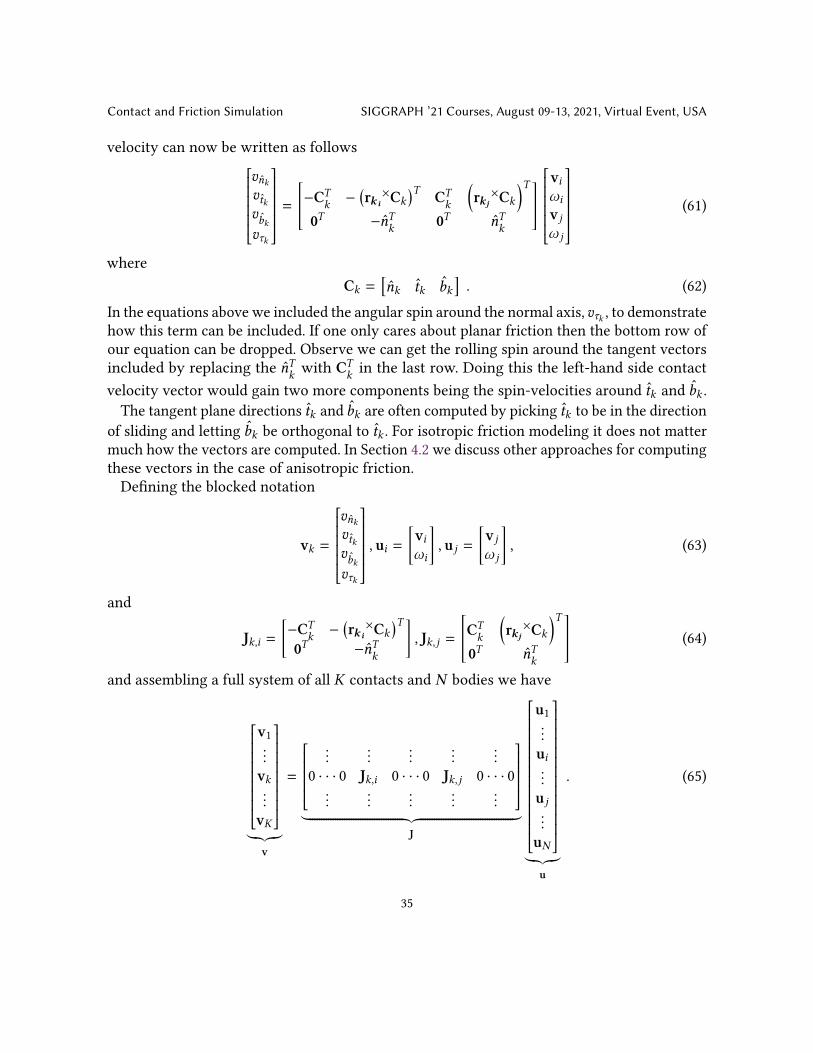
Contact and Friction Simulation SIGGRAPH ’21 Courses, August 09-13, 2021, Virtual Event, USA
velocity can now be written as follows𝑣�̂�𝑘𝑣𝑡𝑘𝑣𝑏𝑘
𝑣𝜏𝑘
=
[−C𝑇
𝑘−
(r𝒌𝒊×C𝑘
)𝑇 C𝑇𝑘
(r𝒌𝒋×C𝑘
)𝑇0𝑇 −�̂�𝑇
𝑘0𝑇 �̂�𝑇
𝑘
] v𝑖𝜔𝑖v 𝑗𝜔 𝑗
(61)
whereC𝑘 =
[�̂�𝑘 𝑡𝑘 𝑏𝑘
]. (62)
In the equations above we included the angular spin around the normal axis, 𝑣𝜏𝑘 , to demonstratehow this term can be included. If one only cares about planar friction then the bottom row ofour equation can be dropped. Observe we can get the rolling spin around the tangent vectorsincluded by replacing the �̂�𝑇
𝑘with C𝑇
𝑘in the last row. Doing this the left-hand side contact
velocity vector would gain two more components being the spin-velocities around 𝑡𝑘 and 𝑏𝑘 .The tangent plane directions 𝑡𝑘 and 𝑏𝑘 are often computed by picking 𝑡𝑘 to be in the direction
of sliding and letting 𝑏𝑘 be orthogonal to 𝑡𝑘 . For isotropic friction modeling it does not mattermuch how the vectors are computed. In Section 4.2 we discuss other approaches for computingthese vectors in the case of anisotropic friction.Defining the blocked notation
v𝑘 =
𝑣�̂�𝑘𝑣𝑡𝑘𝑣𝑏𝑘
𝑣𝜏𝑘
, u𝑖 =[v𝑖𝜔𝑖
], u 𝑗 =
[v 𝑗𝜔 𝑗
], (63)
and
J𝑘,𝑖 =[−C𝑇
𝑘−
(r𝒌𝒊×C𝑘
)𝑇0𝑇 −�̂�𝑇
𝑘
], J𝑘,𝑗 =
[C𝑇𝑘
(r𝒌𝒋×C𝑘
)𝑇0𝑇 �̂�𝑇
𝑘
](64)
and assembling a full system of all 𝐾 contacts and 𝑁 bodies we have
v1...
v𝑘...
v𝐾
︸︷︷︸v
=
...
......
......
0 · · · 0 J𝑘,𝑖 0 · · · 0 J𝑘,𝑗 0 · · · 0...
......
......
︸ ︷︷ ︸J
u1...
u𝑖...
u 𝑗...
u𝑁
︸︷︷︸u
. (65)
35

SIGGRAPH ’21 Courses, August 09-13, 2021, Virtual Event, USA Andrews and Erleben
The 𝑖th rigid body has the center of mass position r𝑖 and the orientation given by the unitquaternion 𝑄𝑖 ≡ (𝜙𝑖,𝜓𝑖, \𝑖, b𝑖) together with the mass𝑚𝑖 and local body-frame inertia tensorIBF𝑖 . The local body frame inertia tensor must be updated to reflect the world-frame inertiatensor
IWF𝑖 = R𝑖IBF𝑖R𝑇𝑖 (66)
where R𝑖 is the rotation matrix corresponding to 𝑄𝑖 . Defining the mass-block notation
M𝑖 =
[𝑚𝑖I3×3 0
0 IWF𝑖
]. (67)
Now the assembled mass matrix reads
M =
M1 . . . 0...
. . ....
0 . . . M𝑁
. (68)
Let fext𝑖 and 𝜏ext𝑖 be the force and torque accumulators of all external force types acting on the𝑖th body. Using the block-notation
f𝑖 =[
fext𝑖𝜏ext𝑖 − 𝜔𝑖 × IWF𝜔𝑖
], (69)
for the external and gyroscopic forces we assemble the f vector,
f =[f𝑇1
... f𝑇𝑁
]𝑇. (70)
Defining the blocked notation
q𝑖 =[r𝑇𝑖 𝑄𝑇𝑖
]𝑇 (71)
then the global assembled version reads
q =[q𝑇1 . . . q𝑇
𝑁
]𝑇. (72)
Notice that the dimension of q and u mismatch and this causes a problem for the generalizedkinematic relation, ¤q = u. The problem can solved introducing the blocked matrix 𝑄𝑖 ≡(𝜙𝑖,𝜓𝑖, \𝑖, b𝑖)
H𝑖 =12
−𝜓𝑖 −\𝑖 −b𝑖𝜙𝑖 b𝑖 −\𝑖−b𝑖 𝜙𝑖 𝜓𝑖\𝑖 −𝜓𝑖 𝜙𝑖
(73)
36

Contact and Friction Simulation SIGGRAPH ’21 Courses, August 09-13, 2021, Virtual Event, USA
and defining
H =
I3×3 0
H𝑖. . .
I3×30 H𝑁
. (74)
The discretized kinematic relation leading to the position update is now given by
q+ = q + Δ𝑡Hu , (75)
which must always be followed by a normalizing of all 𝑄𝑖 ’s to keep them a proper rotation.
1.10.2 Assembling the Matrices for a Soft Body System. For simulation of soft bodies theequations of motion changes slightly as we need to add elastic forces. Elastic forces can becomputed using many different approaches ranging from particle systems to finite elementmethods. A rather large collection of works devoted to elastic body simulation exist in thefield of computer graphics. Below we merely recap a few simple ideas that suffices for us totalk about contact forces for soft bodies and how this is different from the rigid bodies. For amore in depth treatment we refer the interested reader to the SIGGRAPH courses by Sifakisand Barbic [2012] and Kim and Eberle [2020]. For a soft deformable model, the finite elementmethod results in the second order differential equation
M¥q + B¤q + Ku = f + J𝑇λ. (76)
Here q is the concatenation of the positions of all the nodes in the mesh, u is the displacementgiven by the difference from current deformed nodal positions q and undeformed positions q0,and f is the external forces acting on the soft body. The matrixM is the mass matrix of the softbody, B is the damping matrix and K is the stiffness matrix, and J is the contact Jacobian and λcontains the Lagrange multipliers for the contact forces. Observe that if we are in 3D and have𝑁 nodes in a linear tetrahedral mesh then the dimensions of the introduced quantities areq, u, f ∈ R3𝑁 and M,B,K ∈ R3𝑁×3𝑁 . If we have 𝐾 contacts the the J ∈ R3𝐾×3𝑁 and λ ∈ R3𝐾 .We now already observe several differences compared to the rigid body case namely that
there are no orientation or angular spin present in these equations, as such they are simpler aswe do not need to deal with things such as quaternions. On the downside the dimensionality ofthe equation has exploded compared to the rigid body case. A small simple soft body can easilyhave more than 1000 nodes, hence the dimensionality of the equations is at least 2-3 orders ofmagnitude larger. Hence, solving the free motion of soft bodies is much more demanding thanthe rigid body case simply because there are more variables. Lastly we see a new force-type inthe equations, the elastic forces. In our simple setup, we used the most simple type of elasticforce, namely a linear isotropic elastic model. Proper elastic modeling is difficult and thereexist many different elastic models, which one to pick and use is a whole subject in itself. Theelastic forces can be tricky to compute too, but the good news is that the soft elastic nature of
37

SIGGRAPH ’21 Courses, August 09-13, 2021, Virtual Event, USA Andrews and Erleben
the forces numerically dampen the response between nodes in the mesh. That is deformationsin a soft body propagate like a wave through the body. This means that the effect of contactforces too are subject to this wave propagation nature. This is actually how real objects bounce.The nice thing compared to rigid bodies is that the numerics often gets better whereas in rigidbodies all forces in contact are instantly affecting each other, in soft bodies there is a delay,one can say the contact forces act more locally compared to rigid bodies where the effect ismore global on the whole system.We will now perform a typical time discretization using finite difference approximations.
First we observe that time derivative of the velocity is the acceleration, ¤u = ¥q, and so usingfirst order Euler,
¤u ≈ u+ − uℎ
, (77)
where u and u+ are the generalized velocities at time 𝑡 and 𝑡 + ℎ, respectively. Similarly,integrating the generalized positions gives:
q+ ≈ q + ℎu+ . (78)Substituting the above finite difference approximations produces a velocity-level formulationof the dynamics equations, such that
Mu+ − uℎ+ K
(q+ − q0
)+ Bu+ = f + J𝑇λ . (79)
Further manipulation, and converting forces to impulses by 𝝀 = ℎλ, gives the form,
Mu+ −Mu + ℎK(q + ℎu+ − q0
)+ ℎBu+ = ℎf + J𝑇𝝀 . (80)
Finally,Wu+ = w + J𝑇 𝝀, (81)
whereW = M + ℎB + ℎ2K, (82a)w = Mu + ℎ (f − Kq + Kq0) . (82b)
TheWmatrix is sparse block symmetric and positive definite matrix. Thus, if we ignore contactforces momentarily then the linear system can be solved effectively using a numerical methodsuch as the conjugate gradient method. Having found u+ we may do the position update
q+ = q + ℎu+. (83)Adding contact forces to this is straightforward done by adding non-penetration constraintand Coulomb friction law as we have outlined previously. For instance, when setting up theLCP model, we will have the system matrix defined as A ≡ JW−1J𝑇 , and the right-hand-sidevector will be b ≡ JW−1w. If we compare the equations to the rigid body counter part we seethat the change is thatM in the rigid body case is replaced withW in the soft-body case. Whatdoes this imply? ClearlyW is of much higher dimension, and the stiffness matrix K may be
38

Contact and Friction Simulation SIGGRAPH ’21 Courses, August 09-13, 2021, Virtual Event, USA
computational heavy to actual assemble, further the inverse of W is wanted. One remedy is touse a lumped mass matrix and explicit time-discretization of the elastic forces in which caseK drops out from w andW becomes a diagonal matrix. This however is often too limited aslarge time-step sizes causes instabilities in such a semi-implicit time-discretizaton approach.So far, our treatment of the soft body simulation only contained a single soft body when
adding multiple soft bodies to the system the equation of motion is replicated for each softbody. The tricky thing is that different soft bodies can have a different number of nodes and thismeans the block-size will vary when assembling all matrices into one system. As an exampleimagine we are given three soft bodies and their mass matrices areM0,M1, andM2 then thesystem mass matrix will be
M ≡M0 0 00 M1 00 0 M2
. (84)
Here the blocks will be of different size if the number of nodes in the soft bodies are different.Note that if consistent mass matrices are used the assembled mass matrix is not a diagonalmatrix. Similar for the damping and stiffness matrices. The contact Jacobian matrix is slightlydifferent if there are 𝐾 contacts and the number of nodes in the soft bodies are 𝑁0, 𝑁1, and 𝑁2then J ∈ R3𝐾×3 (𝑁0+𝑁1+𝑁2) . Each blocked row will have a form similar to Equation 20.
39

SIGGRAPH ’21 Courses, August 09-13, 2021, Virtual Event, USA Andrews and Erleben
2 CONTACT GENERATIONContact occurs when pairs of bodies touch inside a physics simulation. However, rather thansimply touching, more likely is the scenario where the bodies actually intersect due to someoverlap between their collision geometries. In this section, we discuss methods for generatingcontact points and normals for a variety of geometries.The geometry used to determine whether there is a collision (or not) between two bodies
can have a significant impact on the behavior of contact simulations. Often, performance isa principal consideration when selecting the type of shape used to represent the geometryof a simulation body, in which case simple shapes may be used to approximate the overallshape. We cover those in Section 2.1. However, accuracy and fidelity are also importantconsiderations for certain applications, in which case geometrical representations with moredetail are required, and for such cases we cover mesh-based representations and signeddistances fields in Section 2.2 and Section 2.3 respectively.The algorithms used to detect collisions between shape representations are specific to a pair
of geometries. Throughout this section, we also provide algorithmic details about tests forvarious geometry combinations. In addition to determining whether or not a collision exists,the algorithms must also be extended to compute a contact normal and position. The contactposition is a location that represents the overlapping volume of the two bodies, whereas thecontact normal is the direction of a restorative force that is applied to separate the two bodies.In the case of the normal, it is typically useful to decide on a convention with respect to theorder of bodies. For instance, we assume that contact normals are always directed from thefirst body toward the second body.Essentially a contact point models proximity information between two objects. We label
the objects A and B. Contact points are often used to model touching contact states as well asseparation and penetrating states. The touching state is ideal for giving an intuitive descriptionof the information associated with a contact point. Hence, we will use this state to introduceconcepts. Conceptually a contact point provides three different kinds of information: a position,a normal, and a penetration (gap) measure. For continuous contact regions between twotouching objects there are infinitely many points of contact. Therefore, a contact point canin general be considered as a sample point of those infinitely many points of contact. Formesh-based methods the intersection points between the local mesh features of the two objectsare often used as the contact points.Position: In a touching state a contact point has a reference to the two objects in contact,
and specifies the actual points of the two objects in contact. We describe the common touchingpoint, p ∈ R3 of the two surface points with respect to two objects on the surface of eachobject, p𝐴, p𝐵 ∈ R3. At the ideal touching state, one has p = p𝐴 = p𝐵 . In case of separation orpenetration this equality breaks and one may define p = 1
2 (p𝐴 + p𝐵) or use some weighting ofp𝐴 or p𝐵 based on volume or size of the objects. Positions are used as the point of action when
40

Contact and Friction Simulation SIGGRAPH ’21 Courses, August 09-13, 2021, Virtual Event, USA
applying contact forces, and a consequence of using p𝐴 and p𝐵 is that ghost torques may beintroduced if p𝐴 ≠ p𝐵 .Normal: In a touching state, the surfaces of two smooth objects will have unique parallel
outward unit normals at any shared point on their respective surfaces. Let the two normals be�̂�𝐴, �̂�𝐵 that are oriented in opposite directions, such that �̂�𝐴 = −�̂�𝐵 . Often only one normal �̂�is associated with a contact point. Typically, implementations use a convention to use either�̂� = �̂�𝐴 or �̂� = �̂�𝐵 as the normal associated with a contact point. For the case of penetration,the concept of a normal is perhaps less intuitive. Ideas such as using the minimum distancevector or minimum translational distance may instead be used to define �̂�. To make mattersworse, for non-smooth surfaces, �̂�𝐴 and �̂�𝐵 become indeterminate. Even if they are well-defined, one may not have �̂�𝐴 = −�̂�𝐵 . Nevertheless, the normal is computed and used to applynon-interpenetration forces in the correct direction.Penetration Measure: The penetration is defined to be zero for touching, positive for
separation, and negative for intersection. This follows the same convention of the gap function𝜙 introduced in Section 1. Conceptually, penetration is the distance one would need to movealong �̂� to bring the two objects into a touching state. The measure is often used to addstabilization terms to counter drift errors. Hence, it need not be a distance measure, but somemonotone function that penalizes the constraint violation. For instance, volume overlap couldalternatively be one such measure.
2.1 Analytic Shapes
𝑟
𝐜
𝐜
𝐡
𝐡𝐡
Simple shapes may be used as an approximate representation for thesurface of an object.While they are often used as elements in a hierarchicaldata structure, like bounding volume hierarchies, to perform cheap andconservative intersection tests, they are also commonly used as thefundamental geometry for many collision detection tasks. Implicit surfacerepresentations are common examples of collision proxies, such as spheresand planes. Whereas related surface representations may be used in othercases, such as capsules or boxes. In this section, we consider some of thesesimple shapes– spheres and boxes– and how to generate contacts usingthem.Spheres are perhaps the most efficient 3D shapes for collision tests, bothin terms of storage and computational efficiency. A sphere is defined by acenter point c ∈ R3 and radius 𝑟 ∈ R, as shown in the figure on the right.Boxes are also popular due to their efficiency. Specifically, orientedbounding boxes (OBBs) that follow the local coordinate system of theobject can be adjusted to give a good approximation of the visual geometryof an object. An OBB can be defined by center point c ∈ R3, rotation matrix R ∈ 𝑆𝑂 (3) andhalf-width extents along the local axes h ∈ R3, as shown in the figure on the right.
41

SIGGRAPH ’21 Courses, August 09-13, 2021, Virtual Event, USA Andrews and Erleben
𝐜
𝐜
𝐩
𝑛
𝑟
𝑟
Fig. 10. A sphere-sphere intersection.
2.1.1 Sphere-Sphere Intersection. Assuming that the center position of two spheres sharecommon reference frame, the intersection test involves simply computing the distance betweenthe two centers positions, c1 and c2, and checking if the distance is less than the sum of theradii 𝑟1 and 𝑟2. In other words, if the gap function is negative or zero, such that
𝜙 = ∥c2 − c1∥ − (𝑟1 + 𝑟2) ≤ 0 ,
and if the above condition is true, a contact is generated. The contact normal for a sphere-sphere intersection is aligned with the vector between the two centers, and the unit lengthnormal is computed as
�̂� =c2 − c1
∥c2 − c1∥.
Note that special consideration should be given to the degenerate case where c1 = c2, and inthis case a good option is to simply specify an axis-aligned normal vector. The contact point islocated anywhere along the line connecting the two centers. A common choice is the center ofthe overlapping region:
p =12(c2 − 𝑟2�̂�) +
12(c1 + 𝑟1�̂�)
Other options for computing the contact point include using a radius-weighted sum of thedistance between the centers, or a point on the surface of either sphere.
2.1.2 Sphere-OBB Intersection. The intersection test between a sphere and an OBB requiresfirst transforming the center of the sphere into the local coordinate system of the box:
clocal = R−1OBB(csphere − cOBB)
Then, the closest point g on the box is found by considering the extents h in each axiallyaligned direction, and each coordinate 𝑖 ∈ {𝑥,𝑦, 𝑧} of the closest point is compute as
42

Contact and Friction Simulation SIGGRAPH ’21 Courses, August 09-13, 2021, Virtual Event, USA
𝐜
𝐜
𝐜 𝐑 𝐜 𝐜
𝐠
𝑛
𝐡
𝐡
𝐜𝐠
𝑛𝐡
𝐡
𝐜
shallow penetration deep penetration
Fig. 11. Sphere-OBB intersection showing the shallow (left) and deep (right) penetration. Note thatthe 𝑧-dimension is not shown.
g𝑖 =−h𝑖 , −h𝑖 > clocal,𝑖h𝑖 , h𝑖 < clocal,𝑖clocal,𝑖 , otherwise
(85)
If the distance from the closest point to the sphere center is less than the radius of the sphere,such that ∥g − clocal∥ < 𝑟 , then there is an intersection. However, special consideration mustbe given to the scenario where the sphere center is entirely inside the box, in which caseg = clocal based on Equation 85. Thus, there are two cases to consider when computing thecontact normal: shallow and deep penetration.Shallow penetration occurs if the transformed sphere center lies outside the box extents in
at least one dimension. The penetration 𝜙 is computed as the difference between the distance∥g − clocal∥ and the sphere radius:
𝜙 = ∥g − clocal∥ − 𝑟The normal may be simply computed as the unit vector that points from the sphere center tothe closest point transformed in the global reference frame:
�̂� = ROBBg − clocal∥g − clocal∥
Deep penetration is the case when the transformed sphere center lies entirely inside thebox. This is somewhat of an extreme scenario for contact simulation, but nonetheless shouldbe handled if robust collision is desired. The collision detection algorithm must determinewhich of the box faces is closest to clocal. This is easily tested since the sphere center has beentransformed to the local coordinate system of the box, and the test reduces to determining
43

SIGGRAPH ’21 Courses, August 09-13, 2021, Virtual Event, USA Andrews and Erleben
which axis-aligned distance test returns the minimum penetration:
𝜙 = −min(|h𝑥 − clocal,𝑥 |, |h𝑦 − clocal,𝑦 |, |h𝑧 − clocal,𝑧 |
)It is trivial to determine the closest face by considering the sign of the term that minimizes theabove function. The point g is then computed by projecting the local sphere center onto theclosest face. For example, in Figure 85, the closest point on the box surface is computed bymoving the sphere center to the −𝑥 face, such that
g =[−h𝑥 clocal,𝑦 clocal,𝑧
]𝑇.
Similarly, the normal of the closest box face also determines the contact normal. For example,in the case of the deep penetration example from Figure 85, the local contact normal is
�̂� =[−1 0 0
]𝑇,
and the world space normal is computed as ROBB�̂�. Finally, the contact point for both theshallow and deep penetration case may be located anywhere in the overlapping region betweenthe OBB and the sphere. For simplicity, the closest point on the box is transformed to theglobal coordinate system:
p = ROBBg + cOBB .
2.1.3 OBB-OBB Intersection. Testing for intersection between two OBBs is a special case oftesting for intersection between two convex hulls. There are several algorithms that can beconsidered here, such as the Gilbert–Johnson–Keerthi (GJK) distance algorithm [Gilbert et al.1988] and the separating axis theorem (SAT) [Boyd and Vandenberghe 2004]. The latter isoften preferred since the SAT allows efficient identification of the contact surfaces, as well asthe penetration depth. Although, GJK may be combine with the expanding polytope algorithm(EPA) [Van Den Bergen 2003] to compute the overlap.The first step is to determine if an intersection exists between the boxes. The SAT states that
two convex objects do not intersect if a plane, onto which each the geometry of each convexshape is projected, can be found where they do not overlap. Recall that the orientation of aplane is determined by a normal vector that is perpendicular to the plane. For the OBB-OBBintersection test, the following cases are considered for the separating plane orientation:• The 3 face normals from box A ;• The 3 face normals from box B ;• The 9 normals formed by computing the cross-product of all edge pairs combining box Awith box B.
Given two OBBs A and B, the tests involve projecting the vector between the box centers,d𝐴𝐵 = c𝐵 − c𝐴, onto the separating axis of the plane, 𝑙 . Then, we check if the sum of theprojected box extents exceeds it. Due to symmetry, we can avoid additional tests for thedirectional alignment of vectors by using the absolute value of the projections, which results
44

Contact and Friction Simulation SIGGRAPH ’21 Courses, August 09-13, 2021, Virtual Event, USA
𝐴
𝐵
𝐜
𝐝
𝐡𝐡
𝑙𝐝 ⋅ 𝑙
𝐡 ⋅ 𝑙 𝐡 ⋅ 𝑙
𝐜
Fig. 12. A separating axis test applied to two boxes in 2D. The vector between the box centers, d𝐴𝐵 , isprojected onto the axis 𝑙 , and similarly for the box extents h𝐴 and h𝐵 . Since the sum of the absolutevalues of the projected extents is less than |d𝐴𝐵 · 𝑙 |, there is a separation and hence no collision.
in the separation equation
𝑠 = |d𝐴𝐵 · 𝑙 | −(|h𝐴 · 𝑙 | + |h𝐵 · 𝑙 |
). (86)
If an axis can be found such that 𝑠 > 0, then there is no intersection and thus there is no needto continue. Otherwise, if 𝑠 ≤ 0 for all SAT tests, then an overlap exists and a contact will begenerated.The next step in OBB-OBB intersection requires determining which of the tests resulted in
the shallowest penetration. For this purpose, specific edge pairs and faces giving a minimumseparation are carefully tracked during the overlap tests. Once the test case has been identified,there are two cases to consider for computing the contact normal and point: i) an edge-edgeintersection, or ii) a face intersection.Edge-edge intersection occurs if the shallowest separation is due to a separating planecomputed from an edge-edge pair. In this case, the contact normal is computed as the cross-product of the edges. That is, for edge eA from body A and edge eB from body B, the contactnormal is computed as
�̂� =e𝐴 × e𝐵∥eA × eB∥
. (87)
Note that here we use that convention that edges are vectors between edge vertices. Thenormal is computed assuming all edge vertices are expressed in the global coordinate system,and otherwise the normal must be rotated from the local coordinate system. Only a singlecontact point is generated for an edge intersection. The contact point is computed by findingthe closest points on each edge, such that
p𝐴, p𝐵 ← ClosestPoints (e𝐴, e𝐵) .
45

SIGGRAPH ’21 Courses, August 09-13, 2021, Virtual Event, USA Andrews and Erleben
Finally, the penetration is then computed by as the distance between the closest edge points:𝜙 = −∥p𝐴 − p𝐵 ∥ .
Alternatively, the contact point may be computed as the midpoint of the overlapping region:
p =12(p𝐴 + p𝐵) .
Face intersection occurs between a face of one box and a combination of geometrical featuresfrom the other box (vertices, edges, or faces). However, rather than a single contact point, a faceintersection can generate up to eight contacts depending on the configuration of the bodies.The first step in this case is to determine which of the faces, from either box, resulted in theshallowest penetration. This can be done efficiently by carefully tracking the separation valuesduring the SAT tests and choosing the face that maximizes 𝑠 , assuming that all tests return anegative separation. The responsible face is denoted as the reference face, and so it remains todetermine the incident face on the other box that intersects it. Without loss of generality, letus assume that the reference face belongs to box A. The incident face 𝑓 is found by searchingthe faces of box B for the one that most opposes the reference face. This is achieved by findingthe face on box B whose normal �̂� 𝑓 minimizes the dot product with the reference face normal,�̂�ref, such that
𝑓 = arg min𝑖∈𝐹B
�̂�𝑖 · �̂�ref ,
where 𝐹B are the faces of the box from body B. The incident face is then clipped to the sidesof the reference plane using a polygon clipping algorithm (such as the Sutherland-Hodgmanalgorithm [Sutherland and Hodgman 1974]). For this purpose, a transformation of box B intothe local coordinate system of box A is recommended, since in this reference frame the clippingplanes are all axis aligned. Each clipped edge vertex on the incident face that lies below thereference face plane generates a contact. A 2D example is shown in Figure 13.The normal for each generated contact 𝑗 is the normal of the reference face:
�̂� 𝑗 = �̂�ref
The contact point is found by projecting the clipped edge vertices onto the reference plane,but only for those edges that intersect the plane. Recall that if clipping occurs in the localcoordinate frame of the reference box, then projection simply requires changing one of thecoordinates of the clipped edge vertex to match the position of the reference face. For example,if the reference face normal is +𝑦 from box A, then for clipped edge vertex x̄, the vertexprojected onto the reference face has position
p =[x̄𝑥 hA,𝑦 x̄𝑧
]𝑇,
where the 𝑦 coordinate is assigned h𝑦 from the half-width extend vector of box A. Thepenetration is then computed as the projection distance, which for the +𝑦 face is:
𝜙 = −|x̄𝑦 − h𝑦 | .
46

Contact and Friction Simulation SIGGRAPH ’21 Courses, August 09-13, 2021, Virtual Event, USA
𝐱𝐱
incident face
𝑛
𝑛
reference face 𝑦
clip plane 𝑥 clip plane 𝑥
𝐩 𝐩
Fig. 13. Generation of contacts for OBB-OBB face intersection. This 2D example shows a collisionbetween an edge of the grey box and the +𝑦 face of the blue box. The edge vertices are clipped to theextents of the reference plane, and the clipped vertices are then projected to the reference plane togenerate the contact points p1 and p2.
2.2 Mesh-based RepresentationsIn computer graphics, objects are often represented by polygonal meshes and in particulartriangle meshes are very popular for representing the shape of objects. This section brieflypresents how to compute contact points for such representations.In practical implementations, mesh-based contact generation is done in several stages. In a
first stage, a broad phase collision detection method determines triangles that are sufficientlyclose and which pair-wise triangles need further processing. Often, bounding volume hierar-chies or spatial hashing are the common tools applied in this stage. For the remainder of ourdiscussion on mesh-based contact generation, we assume that these initial stages have beencompleted and instead focus on how the actual contact points are generated.For the mesh-based contact point generation the positions and normals are defined directly
frommesh features such as vertices (𝑉 ), edges (𝐸) or faces (𝐹 ) of the mesh surfaces. For instance,pA and pA can be computed as intersection points of mesh features, or from closest pointsbetween mesh features. As we saw with box-box collisions, normals can be computed froma face normal or as a cross product of two edge vectors. Hence, the types of mesh featuresare often associated with the contact point and used to classify the type of the contact point.For instance, one may write a contact as (𝑉 , 𝐹 ) or (𝐸, 𝐸) to identify a vertex-face generatedcontact point or edge-edge generated contact point, respectively.
47

SIGGRAPH ’21 Courses, August 09-13, 2021, Virtual Event, USA Andrews and Erleben
𝑉,𝐹
𝐸,𝐸
Fig. 14. Corner points of polygonal contact areas can be represented by pairs for mesh features. Thevertex-face (𝑉 , 𝐹 ) and edge-edge (𝐸, 𝐸) combinations forms a sufficient set of pair-types.
The illustration in Figure 14 on the right shows the concept of feature pairs. The blue contactpoints are defined by intersection points of mesh vertices, edges and faces from the two objectsA and B. The drawing has two contact points of type (𝑉 , 𝐹 ) and two contact points of type(𝐸, 𝐸). There is a total of six possible types. They are rarely all used as some of them canbe considered sub-types of each other. For instance, a (𝐹, 𝐹 ) type can be broken down intomultiple (𝑉 , 𝐹 ) type contact points. Associating the mesh features with a contact point has thebenefit of being able to track a contact point over time simply by using labels of features andobjects. Feature labels are convenient to test for redundancy without having to use floatingpoint comparisons.Figure 14 illustrates the ideal case where there is no penetration or separation between
the two objects; they are simply touching. However, due to the nature of the discrete timestepping scheme we introduced earlier in Section 1, it is expected that objects will be slightlyseparated or that penetrations will exist. Hence, it becomes tricky to define what constitutes acontact point. In many practical implementations, it is common to simply take mean positionsof closest points between vertex and face pairs or between edge and edge pairs. The distancebetween closest points is then used as a measure of penetration.
2.2.1 Continuous Collision Detection of Mesh Features. Rather than dealing with the difficultiesthat arise from using a discrete collision detection scheme, a more intelligent approach is touse continuous collision detection (CCD). This type of method processes every collision eventthat might occurs for a given time span (i.e., a time-step). There are two flavors of continuouscollision detection: (i) look forward in time, from the current instance of invocation to the
48

Contact and Friction Simulation SIGGRAPH ’21 Courses, August 09-13, 2021, Virtual Event, USA
next expected instance, or (ii) look backward in time, from the current instance of invocationto the previous instance.The initial stages of CCD often use a time-swept volume around the geometric features of
the mesh-based objects. If the volumes intersect, then a more detailed computation is initiatedto find the time of first contact, at which point one can simply compute normals and contactpoints as outlined above.The CCD can be used in the discrete time-stepping method in many ways. The smallest
computed time-of-impact can be used as a limit on how big a time-step one can use. Alterna-tively, one can take the CCD computed normals and points and warp them to the start of thetime-step. In the case of the latter, a heuristic is required to measure the penetration depth ofan earlier instant.When looking backward in time we are actually seeking the first point of contact. This point
in space is attractive for simulation methods, since it implies the point in time to which weshould “rewind” the simulation in order to avoid penetration. Let us dig a bit deeper into howto predict this point using geometric features of the mesh.Assuming that the time-step is small, it is justifiable that the motion between two instances of
time may be considered linear. However, the errors based on this assumption increase with thesize of the time-step, or O(ℎ). From a convergence theory point of view, we can simply let thetime-step go to zero and the approximation would be exact. In practice, this is impossible, butthe error can be made so small that it is negligible compared to errors coming from numericalinaccuracies and round off. Other assumptions about the motion can sometimes be made, suchthat it is a screw motion, which is commonly done for rigid bodies and can allow for largertime-steps in practice. However, we limit the assumption to linear motion for small time-stepssince the method we outline should be sufficiently general to work for both rigid and softbodies.We can compute the space swept by a single triangle over the time-step. Consider that the
three vertices of a triangle move with velocities u0, u1, and u2. Then, for a forward predictionscheme and based on the linear motion assumption, the triangle will have candidate positionsat the next time step given by
x′0 = x0 + ℎu0, (88a)x′1 = x1 + ℎu1, (88b)x′2 = x2 + ℎu2 . (88c)
However, for a backward prediction scheme, the candidate positions would be
x′0 = x0 − ℎu0, (89a)x′1 = x1 − ℎu1, (89b)x′2 = x2 − ℎu2 . (89c)
49

SIGGRAPH ’21 Courses, August 09-13, 2021, Virtual Event, USA Andrews and Erleben
In the case of backward prediction, we know the exact candidate position without having tocompute them as above. Instead, the linear velocity may be computed as
u0 =x0 − x′0ℎ
, (90a)
u1 =x1 − x′1ℎ
, (90b)
u2 =x2 − x′2ℎ
. (90c)
A simple preliminary test would be to create two axis aligned bounding boxes (AABBs) thatenclose the triangles– one using the current positions and the other using the candidatepositions– and test them for overlap. Only if the bounding boxes overlap can there be a contactthat occurred between the mesh features during the interval ℎ.The next step is to examine all possible contact types for the triangle pair. Specifically, (𝑉 , 𝐹 )
and (𝐸, 𝐸) contacts. In some approaches, like the ones based on bounding volume hierarchies,the triangle pairs are split into sub-types. Whereas for other approaches, like spatial hashing,they work directly with the mesh feature pairs.Due to our assumption of linear motion over the time interval, ℎ, the time of contact is
characterized by either: (i) the vertex lying in the face plane in the case of a (𝑉 , 𝐹 ) contact, or(ii) by two edges being co-planar in the case of an (𝐸, 𝐸) contact. Regardless of the case, weseek a point in time where four points all lie in the same plane.
2.2.2 Continuous Collision Detection of Face-Vertex Pair. The idea is to use three points tocompute a plane normal, and then use one of the three points to find a distance betweenthe plane and the origin. Finally, the fourth point is used for a point in the plane test. Forconvenience, in the case of the (𝑉 , 𝐹 ), let us label the points of the triangle in counterclockwiseorder: x1, x2, and x3 and the point of the vertex x4. In the case of an (𝐸, 𝐸) type, we label theend-points of the first edge x1 and x2, and the end-points of the second edge x3 and x4. Thecorresponding velocities are in both cases labeled u1, u2, u3, and u4. Now we’ll set up twovectors x2 − x1 and x3 − x1, and take the cross product of these two to obtain a plane normal
�̂� = ((x2 − x1) × (x3 − x1) . (91)
The point x1 must lie in the plane, so the distance, 𝑑 , to the origin is given by
𝑑 = �̂� · x1. (92)
In order for the last point to lie in the plane, then its distance to the plane must be zero, that is,
�̂� · x4 − 𝑑 = 0 . (93)
Substitution leads to((x2 − x1) × (x3 − x1)) · (x4 − x1) = 0. (94)
50

Contact and Friction Simulation SIGGRAPH ’21 Courses, August 09-13, 2021, Virtual Event, USA
Whenever this equation is fulfilled, the four points will lie in the same plane. The last thing toconsider is the motion of the points whose positions change with time, such that
((x2(𝑡) − x1(𝑡)) × (x3(𝑡) − x1(𝑡))) · (x4(𝑡) − x1(𝑡)) = 0 . (95)
Here, the objective is to determine the smallest non-negative value 𝑡 < ℎ that makes the aboveequation true. From the linear motion assumption, the trajectory of each point may be writtenas
x1(𝑡) = x1 + u1𝑡, (96a)x2(𝑡) = x2 + u2𝑡, (96b)x3(𝑡) = x3 + u3𝑡, (96c)x4(𝑡) = x4 + u4𝑡 , (96d)
and by substitution we obtain
(((x2 − x1) + (u2 − u1) 𝑡) × ((x3 − x1) + (u3 − u1) 𝑡)) · ((x4 − x1) + (u4 − u1) 𝑡) = 0 . (97)
This is a cubic polynomial with an analytical solution. Once the three roots are found, thepositions of the vertices can also be found at the specific values of 𝑡 . Note that a roundingerror may hide a collision at the boundary between two time-steps, and a test at the end of thetime-step 𝑡 = ℎ should therefore by performed [Bridson et al. 2002].Having found the earliest point in time where the four points are co-planar, we will finally
compute the candidate for the contact point p = x4 + u4𝑡 , if this point is inside the triangle facethen a contact point is reported with position p, normal n = (x2(𝑡) − x1(𝑡)) × (x3(𝑡) − x1(𝑡))and penetration depth of 𝜙 = 0. In most simulation approaches the state will be reset to theearliest point in time where a collision is found hence the penetration depth will always bezero.
2.2.3 Continuous Collision Detection of Edge-Edge Pair. As in the (𝑉 , 𝐹 ) case, the (𝐸, 𝐸) caserequires finding the roots of a polynomial equation, and then examining the geometries inascending temporal order. For simplicity, let x1, x2, x3, and x4 denote the edge geometrypositions at the instant in time corresponding to a root. First, we test whether the edges areparallel. This is the case when
(x2 − x1) × (x4 − x3) = 0 . (98)
In practice, an equality test will not work, so we use a threshold test instead. If the test succeeds,then a dimension reduction technique can be used by projecting the vertices of one edge ontothe line running through the edge. However, one could also simply drop this case, since ifa touching contact exists, it could just as well be represented by two (𝑉 , 𝐹 ) type contacts.Therefore, we will only consider the case where the two edges are touching at exactly onepoint.
51
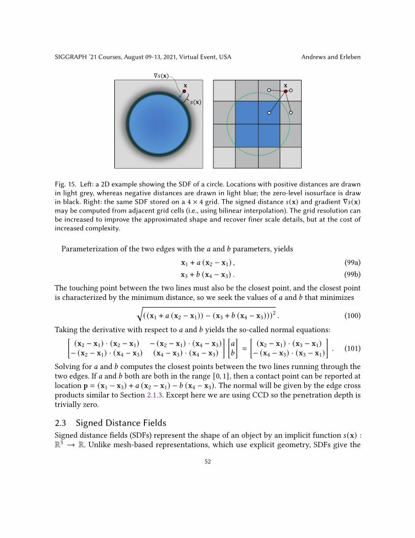
SIGGRAPH ’21 Courses, August 09-13, 2021, Virtual Event, USA Andrews and Erleben
𝐱
𝑠 𝐱
∇𝑠 𝐱𝐱
Fig. 15. Left: a 2D example showing the SDF of a circle. Locations with positive distances are drawnin light grey, whereas negative distances are drawn in light blue; the zero-level isosurface is drawin black. Right: the same SDF stored on a 4 × 4 grid. The signed distance 𝑠 (x) and gradient ∇𝑠 (x)may be computed from adjacent grid cells (i.e., using bilinear interpolation). The grid resolution canbe increased to improve the approximated shape and recover finer scale details, but at the cost ofincreased complexity.
Parameterization of the two edges with the 𝑎 and 𝑏 parameters, yields
x1 + 𝑎 (x2 − x1) , (99a)x3 + 𝑏 (x4 − x3) . (99b)
The touching point between the two lines must also be the closest point, and the closest pointis characterized by the minimum distance, so we seek the values of 𝑎 and 𝑏 that minimizes√︃
((x1 + 𝑎 (x2 − x1)) − (x3 + 𝑏 (x4 − x3)))2 . (100)
Taking the derivative with respect to 𝑎 and 𝑏 yields the so-called normal equations:[(x2 − x1) · (x2 − x1) − (x2 − x1) · (x4 − x3)− (x2 − x1) · (x4 − x3) (x4 − x3) · (x4 − x3)
] [𝑎
𝑏
]=
[(x2 − x1) · (x3 − x1)− (x4 − x3) · (x3 − x1)
]. (101)
Solving for 𝑎 and 𝑏 computes the closest points between the two lines running through thetwo edges. If 𝑎 and 𝑏 both are both in the range [0, 1], then a contact point can be reported atlocation p = (x1 − x3) + 𝑎 (x2 − x1) − 𝑏 (x4 − x3). The normal will be given by the edge crossproducts similar to Section 2.1.3. Except here we are using CCD so the penetration depth istrivially zero.
2.3 Signed Distance FieldsSigned distance fields (SDFs) represent the shape of an object by an implicit function 𝑠 (x) :R3 → R. Unlike mesh-based representations, which use explicit geometry, SDFs give the
52

Contact and Friction Simulation SIGGRAPH ’21 Courses, August 09-13, 2021, Virtual Event, USA
signed distance of some point x from the surface of an object. The sign (positive or negative)indicates whether the point lies outside or inside of the object. Specifically, points interior tothe shape have 𝑠 (x) < 0, whereas exterior points have 𝑠 (x) > 0, and points on the surfacesatisfy 𝑠 (x) = 0. For example, the SDF of a circle is shown on the left side of Figure 15, anddifferent colors are used to draw regions with positive and negative distances and the zero-levelisosurface.In this section, we present some details about performing collision detection and generating
contacts using SDFs. Specifically, we show how polygonal meshes can be tested for intersectionusing SDFs. This offers an alternative to the mesh-mesh based collision detection outlined inSection 2.2, since it is straightforward to generate an SDF from a polygon mesh that can thenbe used for efficient collision detection. However, we do not cover how to generate SDFs, andinstead refer the reader to related work on this topic [Jones et al. 2006].In addition to computing a scalar field of signed distances, is it also common to compute
its gradient, ∇𝑠 (x) ∈ R3. Observe that the gradient function returns a 3D vector that givesdirection of the closest point on the surface from x. A desirable property of the gradientfunction is that the returned vector is unit length, such that
∥∇𝑠 (x)∥ = 1 .
Therefore, ∇𝑠 (x) in fact gives the vector field of inward facing unit normal vectors. However,this property of the field may not always be true, for instance if the closet point is not unique(e.g., the center of a sphere), but in practice the gradient function can be constructed so as topreserve this property.
2.3.1 SDF-Point Intersection. The canonical intersection test using an SDF is with a point. Thefirst step is to determine if 𝑠 (x) ≤ 0 is true, which means that either x is an interior point ortouching the surface. If true, the gap function 𝜙 is simply the signed distance provided by thefield function:
𝜙 = 𝑠 (x) (102)
Next, let us consider how to compute the contact normal. Generally speaking, the normal isgiven by the forcing direction that will most quickly move x outside the field. This is in factthe gradient evaluated at x, and so the contact normal may be computed as:
�̂� = −∇𝑠 (x)𝑇 (103)
Note again that special care should be taken to orient the normal based on the conventionused by the collision system (e.g., from the first body toward the second body).Finally, there are two obvious choices for computing the contact position. One option is to
situate the contact point p at the surface of the SDF, which is computed by projecting x alongthe gradient:
p = x − ∇𝑠 (x)𝑇𝑠 (x) (104)
53

SIGGRAPH ’21 Courses, August 09-13, 2021, Virtual Event, USA Andrews and Erleben
Input: mesh 𝐹,𝑉 , SDF 𝑠 , gradient field ∇𝑠Result: List of contacts C
1 ∀x ∈ 𝑉2 compute xlocal by transforming x (Equation 106)3 if 𝑠 (xlocal) < 0 then4 𝜙 = 𝑠 (xlocal)5 �̂� = ∇𝑠 (xlocal)𝑇6 p = x7 transform �̂� and p to world coordinates8 C← C ∪ {�̂�, p, 𝜙}9 end
Algorithm 1: SDF-Mesh contact generation
Conversely, the query point may be used, such thatp = x . (105)
2.3.2 SDF-Mesh Intersection. Generating a contact for the SDF and point intersection providesa useful building block for collision with more complex geometries, such as polygonal meshes.Collision detection between meshes can be computationally costly, as we saw in Section 2.2.However, a common use case of SDFs is accelerating mesh-mesh collision detection bycomputing a signed distance field for each mesh and then performing approximate intersectiontests using the SDF of one object versus the mesh of the other. Luckily, there are robust methodsfor building an SDF from arbitrary polygonal soups [Xu and Barbič 2014].In Section 2.3.1, we saw that it is straightforward to generate contacts for the case of a
point intersecting an SDF. This naturally leads to an intersection test with a polygonal mesh,whereby each vertex x ∈ 𝑉 is tested. Let us assume that we want to test a vertex from themesh of body B with the signed distance field of body A. The first step is to transform vertex vinto the local coordinate system of body A, since it is often more efficient to transform themesh vertices into the field coordinate frame, rather than the other way around. A local vertexposition is computed, such that
xlocal = R−1A (RB (x + cB) − cA) , (106)
where cA ∈ R3, RA ∈ 𝑆𝑂 (3) and cB ∈ R3, RB ∈ 𝑆𝑂 (3) are the positions and rotation matricesof bodies A and B respectively. Then, if 𝑠 (xlocal) < 0, an intersection exists and Equation 102-Equation 105 may be used to generate the depth, contact normal and position. This process issummarized in Algorithm 1.However, testing only against the vertices of the polygonal mesh can lead to missed collisions
and other artifacts. For instance, this is likely if the mesh geometry is coarse and the SDFsurface contains thin features. These issues can be mitigated by adding more vertices to the
54

Contact and Friction Simulation SIGGRAPH ’21 Courses, August 09-13, 2021, Virtual Event, USA
mesh, although theoretically this will never fully eliminate penetration artifacts and may alsoimpact performance.Recently, Macklin et al. [2020a] proposed a refinement technique to compute exact collision
between SDFs and polygonal meshes. Rather than considering each vertex of the mesh, eachface is considered. Assuming a triangle mesh, each face is defined by vertices x1, x2, x3 ∈ R3. Apoint on the interior or boundary of the face can be described by its barycentric coordinates𝑢, 𝑣,𝑤 , such that
x(𝑢, 𝑣,𝑤) = 𝑢x1 + 𝑣x2 +𝑤x3 , (107a)subject to 𝑢, 𝑣,𝑤 ≥ 0 , (107b)
𝑢 + 𝑣 +𝑤 = 1 . (107c)The closest point on the face can then be found by a minimization over the barycentriccoordinates:
arg min𝑢,𝑣,𝑤
𝑠 (𝑢x1 + 𝑣x2 +𝑤x3) (108)
The minimization in Equation 108 is a non-linear optimization problem, and thus requires aniterative approach. For instance, a projected gradient descent method. However, this requirescomputing the derivative of the distance field at each candidate solution with respect to thebarycentric coordinates, which is
d =
𝜕s𝜕𝑢𝜕s𝜕𝑣𝜕s𝜕𝑤
=
∇𝑠 (x)x1∇𝑠 (x)x2∇𝑠 (x)x3
.At the 𝑘th iteration of the gradient descent algorithm, the candidate solution to Equation 108is then updated by a fixed-point iteration, such that
x(𝑘+1) ← ProjBarycentric(x(𝑘)) − 𝛼d .Here, 𝛼 is a fixed step size and ProjBarycentric projects the solution 𝑢, 𝑣,𝑤 to the manifolddefined by Equation 107b-Equation 107c. After the solver terminates, if 𝑠 (x(𝑢, 𝑣,𝑤)) < 0 thena contact is generated.
2.3.3 Implementation Notes. In practice, an SDF is often represented by a discrete datastructure, such as a dense or sparse voxel grid. Each grid cell (𝑖, 𝑗, 𝑘) stores the signed distance,and thus 𝑠 (x) is computed by first identifying the grid cell containing x and then performingan interpolation using the neighboring grid cells (see the right side of Figure 15). In the caseof the gradient, ∇𝑠 (x), it may be computed on-demand using finite differences, by analyticgradients, or precomputed and stored alongside distance values on the grid.The grid cell size will have an effect on the quality of the collision detection, and often the
grid cell size is determined based on the smallest features of the source geometry. However,this may result in heavy memory consumption if a uniform grid is used to store complexsurfaces. Frisken et al. [2000] proposed an adaptive SDF to address this problem, where an
55

SIGGRAPH ’21 Courses, August 09-13, 2021, Virtual Event, USA Andrews and Erleben
octree subdivision is used to recursively refine the grid until the interpolated field valuesclosely match the original surface. Similarly, Koschier et al. [2016] improved the accuracy ofSDFs for complex geometry by adaptively refining the resolution of the grid, as well as thepolynomial degree used to represent local field details.It is trivial to extend the contact generation techniques presented in this section to analytical
shapes, such as spheres. However, in the case that the field is stored using a discrete grid, it isimportant that the grid is extended by a margin around the zero-level isosurface of the sourcegeometry to avoid discontinuities and ensure that valid field data exists for possible querypoints.
56

Contact and Friction Simulation SIGGRAPH ’21 Courses, August 09-13, 2021, Virtual Event, USA
3 NUMERICAL METHODSIn this section, we present a collection of numerical methods for solving the frictional contactproblems. These can be roughly classified into two general approaches: i) pivoting methodsand ii) iterative methods. Pivoting methods focus on determining a labeling of variablesbased on the complementarity conditions. Once the labeling is known, an exact solutionto the complementarity problem may be computed if a direct solver is used to solve theresulting subproblem. Conversely, iterative methods make incremental progress toward theexact solution, with better approximations being obtained at each iteration. Additionally, thereare hybrid approaches that combine these schemes.The fundamental goal of applying these numerical methods is to solve for the constraint
impulses _, while also ensuring that the feasibility and complementarity conditions of thevarious contact models are met. However, some of the frictional contact models from Section 1require computing other parameters that are important for producing the correct behavior,such as the slack 𝛽 parameter used by the polyhedral LCP. Therefore, we depart from earlierconvention and now use x to denote the vector of unknowns that is computed by each numericalmethod, rather than just the constraint impulses 𝝀.
3.1 Pivoting MethodsPivoting methods exploit the combinatorial nature of complementarity problems to find alabeling of the variables based on the complementarity and feasibility conditions imposed bythe model. With this labeling, which is sometimes referred to as the index set, it is possible toidentify constraint variables as being free or tight, and the latter case is further decomposedinto tight lower and tight upper variables. This labeling permits a partitioning of linear systembased on the index set. For instance,
AF,F AF,L AF,UAL,F AL,L AL,UAU,F AU,L AU,U
xFxLxU
+bFbLbU
=
vFvLvU
, (109)
where F is the set of free variables, L is the set of tight lower variables, and U is the set of tightupper variables. Each sub-block of A in Equation 109 thus corresponds to selecting rows andcolumns of the lead matrix that correspond to the rows and columns of each set. For instance,AF,L contains row indices from F and column indices from L. The rows of vectors b, x, and vmay be similarly partitioned according to the index set labels.For contact problems, the index set of each variable is determined by inspection of each 𝑣𝑖
and 𝑥𝑖 . Variables in 𝑖 ∈ F are those for which the value of x𝑖 is not restricted by the feasibility
57

SIGGRAPH ’21 Courses, August 09-13, 2021, Virtual Event, USA Andrews and Erleben
condition of the constraint (e.g., the lower and upper bounds). Whereas tight variables 𝑖 ∈ L∪Uhave a value which is determined by the feasibility conditions.1To better understand how this partitioning works, let us consider the BLCP formulation,
where x = 𝝀 are the constraint impulses. From Equation 41, we can define the index sets basedon the feasibility and complementarity conditions of the BLCP based on three cases:
{∀𝑖 ∈ F : _lo𝑖 < _𝑖 < _hi𝑖 and 𝑣𝑖 = 0} , (110a)
{∀𝑖 ∈ L : _𝑖 = _lo𝑖 and 𝑣𝑖 > 0} , (110b)
{∀𝑖 ∈ U : _𝑖 = _hi𝑖 and 𝑣𝑖 < 0} . (110c)
For non-interpenetration constraints, which are only lower bounded, this labeling implies that
𝑖 ∈ F ⇒ _𝑖 > 0 and 𝑣𝑖 = 0 , (111a)𝑖 ∈ L ⇒ _𝑖 = 0 and 𝑣𝑖 > 0 . (111b)
Whereas for frictional constraints with box limits, the free and tight labels imply that
{𝑖 ∈ F ⇒ −`_�̂� < _𝑖 < `_�̂� and 𝑣𝑖 = 0} , (112a){𝑖 ∈ L ⇒ _𝑖 = −`_�̂� and 𝑣𝑖 > 0} , (112b){𝑖 ∈ U ⇒ _𝑖 = +`_�̂� and 𝑣𝑖 < 0} , (112c)
where _�̂� is the non-interpenetration impulse corresponding to frictional impulse _𝑖 .Extending the conditions in Equations 110a-110c to the general case, we observe that the
residual velocity is zero for all variables in the free set. That is,
∀𝑖 ∈ F : 𝑣𝑖 = 0 .
Furthermore, we note that the value of tight variables is determined by a boundary condition(i.e., they are known). This allows us to simplify Equation 109 to a version that involves onlythe unknown free variables:
AF,FxF = −bF − AF,LxloL − AF,UxhiU (113)
Hence, computing xF simply requires solving an unconstrained linear system. The objectiveof pivoting methods is therefore to correctly determine the index set of constraint variablesthat solves the complementarity problem. Essentially, a solution is found by "guessing" anindex set for the constraint variables and then confirming that a candidate solution is correctwith respect to the complementarity and feasibility conditions. We note that a brute forceapproach for determining the correct index set would be inefficient since it requires guessing2𝑚 possibilities for an𝑚 variables system. Rather, most pivoting methods use a systematic1The variables our contact models are mostly limited by inequality conditions. So, “tight” describes a variablethat is directly against the hyperplane defining an inequality constraint, whereas “free” variables are not andthey have some room on all sides.
58

Contact and Friction Simulation SIGGRAPH ’21 Courses, August 09-13, 2021, Virtual Event, USA
approach to change the index set of individual variables. In the next sections, we will exploresome popular algorithms that use various strategies to pivot variables between the free andtight sets to find a solution.
3.1.1 Incremental Pivoting. Lemke’s algorithm [Lloyd 2005] is a well-known pivoting methodthat incrementally pivots variables between the tight and free set in order to find a basis thatsolves the LCP. The simplex method proposed by Cottle and Dantzig [Cottle 1968] has likewisebeen used to find the index set. Baraff [Baraff 1994] used an incremental pivoting approachbased on Dantzig’s algorithm to solve for contact forces. Their method incrementally computesa solution by making change to the index sets while keeping the complementarity constraintsas invariants. We consider the case of solving a traditional LCP with the index sets followingEquation 111.The algorithm begins with sets F and L empty; set U is ignored. It is presumed that, at
each pivoting step, the complementarity conditions of all previously processed variables aremaintained. The algorithm proceeds at each step by selecting the candidate variable with index𝑗 from the unprocessed set P that minimizes 𝑣 𝑗 ∈ R, since this corresponds to an index withthe most violated complementarity condition. At the 𝑘 th iteration, the following partitioningof the system is used:
v𝑘Fv𝑘L𝑣𝑘𝑗
=
AF,F AF,L AF, 𝑗A𝑇F,L AL,L AL, 𝑗
A𝑇F, 𝑗 A𝑇L, 𝑗 A 𝑗, 𝑗
x𝑘Fx𝑘L0
+bFbL𝑏 𝑗
.Initially, it is assumed that 𝑥 𝑗 = 0. Knowing that x𝑘 of the processed indices respects thecomplementarity conditions, we focus on computing an update of the variables based on achange of the unprocessed variable Δ𝑥 𝑗 , such that
ΔvFΔvLΔ𝑣 𝑗
=
AF,F AF,L AF, 𝑗A𝑇F,L AL,L AL, 𝑗
A𝑇F, 𝑗 A𝑇L, 𝑗 A 𝑗, 𝑗
ΔxFΔxLΔ𝑥 𝑗
.The method takes advantage of the invariants vF = 0 and xL = 0, which logically leads to theassumption that ΔvF = 0 and ΔxL = 0. For a unit increase Δ𝑥 𝑗 = 1, we can write the linearsystem as:
0ΔvLΔ𝑣 𝑗
=
AF,F AF,L AF, 𝑗A𝑇F,L AL,L AL, 𝑗
A𝑇F, 𝑗 A𝑇L, 𝑗 A 𝑗, 𝑗
ΔxF01
. (114)
The first block row of Equation 114 allows us to compute changes in the free variables bysolving
AF,FΔxF = −AF, 𝑗 .
The change in residual velocity of tight variables vL is then given byΔvL = A𝑇F,LΔxF + AL, 𝑗 ,
59

SIGGRAPH ’21 Courses, August 09-13, 2021, Virtual Event, USA Andrews and Erleben
and likewiseΔ𝑣 𝑗 = A𝑇F, 𝑗ΔxF + A 𝑗, 𝑗 .
However, we note that our assumptions are valid only if the index set of variables does notchange. For some 𝑖 ∈ F where Δ𝑥𝑖 < 0, it is possible that 𝑥𝑖 will be driven to zero, in whichcase 𝑖 should be pivoted from F → L. Similarly, for some 𝑖 ∈ L where Δ𝑣𝑖 < 0, it is possiblethe residual velocity 𝑣𝑖 is driven to zero, in which case the variable 𝑖 should be pivoted fromL→ F.Essentially, the idea here is to increase 𝑥𝑘+1𝑗 as much as possible without breaking the
complementarity or feasibility conditions. At each iteration, it is therefore necessary to computea maximum step size 𝛼 up to the point that the index set of one of the variables changes (pivots).Starting with the unprocessed variable 𝑗 , the largest step we can take without forcing 𝑥𝑘+1𝑗
negative is
𝛼 𝑗 =
(−𝑣𝑘𝑗Δ𝑣 𝑗
). (115)
For each 𝑖 ∈ F, if Δ𝑥𝑖 < 0, the minimum step size that can be taken without forcing 𝑥𝑘+1𝑖
negative is
𝛼F = min𝑖∈F∧Δ𝑥𝑖<0
(−𝑥𝑘𝑖Δ𝑥𝑖
). (116)
Finally, for each 𝑖 ∈ L, if Δ𝑣𝑖 < 0, the minimum step size that can be taken without forcing𝑣𝑘+1𝑖 negative is
𝛼L = min𝑖∈L∧Δ𝑣𝑖<0
(−𝑣𝑘𝑖Δ𝑣𝑖
). (117)
The step size is computed as 𝛼 = min(𝛼F, 𝛼L, 𝛼 𝑗
). The constraint impulses are then increased
by 𝛼Δx = 𝛼[ΔxF 0 1
]𝑇 , which causes 𝑣 to change by 𝛼Δ𝑣 = A(𝛼Δx). If the blockingconstraint index is not 𝑗 , this causes a change in the index set and the variable is pivoted tomaintain the complementarity conditions. The process of updating the constraint variables andincreasing Δ𝑥 𝑗 continues until 𝑣 𝑗 is driven to zero. Pseudo-code for the incremental pivotingalgorithm is provided in Algorithm 2.
3.1.2 Principal Pivoting Methods. Unlike Baraff’s incremental pivoting approach, other pivot-ing algorithms initialize variables with a specific label. The Bard-type method proposed byMurty [Murty 1974; Murty and Yu 1988] is one such algorithm, and it uses principal pivots ateach iteration to change the index set whenever a variable at index 𝑖 violates the feasibility orcomplementarity conditions.
60

Contact and Friction Simulation SIGGRAPH ’21 Courses, August 09-13, 2021, Virtual Event, USA
Data: A: The LCP coefficient matrix, b: The right hand side vector.Result: x: The LCP solution, F,L: The index sets of the free and tight variables.
1 x = 02 v = b3 initialize F = L = ∅4 while ∃ 𝑗 such that 𝑣 𝑗 < 0 do5 repeat6 solve AF,FΔxF = −AF, 𝑗
7 ΔvL = A𝑇F,LΔxF + AL, 𝑗
8 Δ𝑣 𝑗 = A𝑇F, 𝑗ΔxF + A 𝑗, 𝑗
9 compute 𝛼 according to Equation 115-Equation 11710 store blocking constraint index 𝑙11 xF ← xF + 𝛼ΔxF12 vL ← vL + 𝛼ΔvL13 _ 𝑗 = 𝛼
14 if 𝑙 ∈ F then15 F← F − {𝑙}16 L← L ∪ {𝑙}17 else if 𝑙 ∈ L then18 L← L − {𝑙}19 F← F ∪ {𝑙}20 else21 F← F ∪ {𝑙}22 until 𝑙 = 𝑗 ;23 end
Algorithm 2: Incremental pivoting for an LCP.
The algorithm begins with an initial “guess” for the index sets, and at each step the principalsub-problem in Equation 113 is solved in order to determine xF, and thus vL and vU too. Ifa variable violates its feasibility or complimentarity conditions, then the algorithm stopssince the current index set is a solution to the LCP. Otherwise, Murty’s algorithm chooses aninfeasible variable with the smallest index 𝑖 and pivots it into the complementary set. That is,
61

SIGGRAPH ’21 Courses, August 09-13, 2021, Virtual Event, USA Andrews and Erleben
variables are pivoted according to the rules:F← F − {𝑖} L = L ∪ {𝑖}, if 𝑖 ∈ F and𝑥𝑖 ≤ 𝑥 lo𝑖F← F − {𝑖} U = U ∪ {𝑖}, if 𝑖 ∈ F and𝑥𝑖 ≥ 𝑥hi𝑖U = U − {𝑖} F← F ∪ {𝑖}, if 𝑖 ∈ U and 𝑣𝑖 ≥ 0L = L − {𝑖} F← F ∪ {𝑖}, if 𝑖 ∈ L and 𝑣𝑖 ≤ 0
. (118)
It can be proven that if the lead matrix A ∈ R𝑛×𝑛 is a P-matrix then the system will finda solution in 𝑛 pivots. However, for degenerate systems, it can be shown that the pivotingalgorithm may lead to cycling, which occurs whenever the same index set is encounteredtwice by the pivoting algorithm. Robust implementations of principal pivoting algorithmsoften require some way to detect and break cycles.
3.1.3 Block Principal Pivoting. Both the incremental pivoting and the Bard-type algorithmproceed at each step by updates that are based on a single variable. While single pivotingschemes have good convergence guarantees, computation times are protracted due to onlychanging a single variable at each step. However, in practice, it is often possible to pivot morethan one variable to achieve faster convergence.Judice and Pires [Júdice and Pires 1994] proposed a block version of Murty’s algorithm
whereby all variables in violation of the feasibility or complementarity conditions are pivotedtogether at each step, rather than just the least indexed variable. Therefore, at each algorithmstep, a pass over all variables check if any violate the condition, and if so the pivotingrules in Equation 118 are applied to all variables in violation simultaneously. The algorithmterminates with success if the index sets between two consecutive pivoting steps do not change.Pseudocode for the block principal pivoting algorithm is provided in Algorithm 3.In practice, the BPP algorithm can converge to the correct index set after only a small number
of iterations. However, cycling in the index set can occur even when A is positive definite. Insuch cases, one strategy proposed by Judice and Pires [Júdice and Pires 1994] is to temporarilyrevert to a Murty single pivoting scheme by choosing an infeasible variable with the leastindex. However, in general, robust implementations of pivoting algorithm require some sort ofcycle breaking strategy.
3.1.4 Implementation Notes. Observe that both the incremental pivoting and the block princi-pal pivoting methods require a solution involving the linear system AF,FxF. We assume thatA is symmetric positive definite (PD), and therefore A−1
FF exists. However, Baraff reportedthat even when A is positive semi-definite (PSD), which is often the case in practice due toredundant contact constraints, then A−1
F,F could still be computed. Applying the constraintstabilization techniques presented in Section 1.9 can improve the conditioning of AF,F andalleviate problems related to degenerate matrices.In practice, forming and solving the linear system uses a Cholesky decomposition. Baraff
noted that for complex systems, an incremental factorization is preferred for efficiency, although
62

Contact and Friction Simulation SIGGRAPH ’21 Courses, August 09-13, 2021, Virtual Event, USA
Data: 𝑁 : The total number of pivoting steps to perform, A: The coefficient matrix, b:The right hand side vector.
Result: x: The BLCP solution for all 𝑛 variables, F,L,U: The index sets of the free andtight variables.
1 initialize F = {1, . . . , 𝑛} , L = ∅ ,U = ∅2 𝑘 = 13 while (𝑘 ≤ 𝑁 and F, L,U changed) do4 ∀ 𝑖 ∈ L : 𝑥𝑖 ← 𝑥 lo𝑖5 ∀ 𝑖 ∈ U : 𝑥𝑖 ← 𝑥hi𝑖6 solve AF,FxF = −bF − AF,LxloL − AF,UxhiU7 v = Ax + b8 update F, L,U according to Equation 1189 𝑘 = 𝑘 + 1
10 end
Algorithm 3: Block principal pivoting (BPP) for BLCPs.
an implementation is potentially non-trivial. Enzenhoefer et al. [2019] proposed an efficientversion of Judice’s block pivoting algorithm that re-uses an initial factorization of AF,FxFand downdates the factorization based on indices in L ∪ U. For complex simulations, theyobserved a 1.5 to 3 times reduction in the computation time of the BPP algorithm when usinga downdated factorization, with the caveat that the approach is more efficient only when anominal percentage of variables is pivoted. Furthermore, parallelization of pivoting methods ischallenging, especially if a factorization is used to solve the principal sub-problem. However,there is some work that has addressed this problem. For instance, Peiret et al. [2019] introduceda parallelization technique for pivoting solvers using a domain decomposition technique, andtheir method is capable of producing exact solutions for the contact BLCP.
3.2 Fixed-point methodsIn this section we will focus on a popular class of methods for solving contact problems thatare commonly referred to as fixed-point methods. Specifically, we focus on the projectedGauss-Seidel (PGS) algorithm and its variants. Furthermore, this section focuses entirely oncontact models that originate from the complementary problem formulations introduced inSections 1.6-1.8. First, we introduce the idea of splitting up the contact problem in order to geta group of more manageable problems, which we can then solve iteratively. This naturallyleads to a frictional contact formulation that can be solved using the PGS method. Then, inSection 3.2.4, the idea of splitting in a recursive fashion is used to derive the blocked Gauss-Seidel method. The staggering method is presented in Section 3.2.5. Blocking and staggeringare general concepts that can be applied in other problem domains, as they serve as a general
63

SIGGRAPH ’21 Courses, August 09-13, 2021, Virtual Event, USA Andrews and Erleben
scheme for combining different numerical solvers into one overall solver. The PGS type ofmethods are interesting building blocks for many other types of numerical methods such assub-space minimization [Silcowitz et al. 2010b] and non-smooth non-linear conjugate gradient(NNCG) method [Silcowitz et al. 2010a]. We cover these higher-level solvers once we havecreated a strong foundation for the PGS type of methods.
3.2.1 Splitting Methods. We begin with the general concept of splitting methods. This class ofmethods is well known in numerical optimization, and includes methods such as Gauss-Seidel,Jacobi and successive over-relaxation (SOR). Splitting methods are iterative methods, whichunlike the pivoting methods described in Section 3.1, are practically incapable of computingthe exact solution to the LCP. Iterative methods approximate the solution, but do so in a muchmore efficient way, both computationally and storage wise. The traditional form of the LCP is
Ax + b ≥ 0 , (119a)x ≥ 0 , (119b)
x𝑇 (Ax + b) = 0 , (119c)
which corresponds to the LCP introduced using the polyhedral cone in Section 1.6. Splittingmethods start with the decomposition of the lead matrix such that A = M − N. Note thatM here is not the mass matrix, and we leave M and N unspecified for now. Using the newdefinition of A, Equation 119 becomes
Mx − Nx + b ≥ 0 , (120a)x ≥ 0 , (120b)
x𝑇 (Mx − Nx + b) = 0 . (120c)
Let us next assume that we will use an iterative method where x𝑘 → x𝑘+1 for 𝑘 → ∞. Thisassumes there is an accumulation or limiting point for the system. We can then rewrite Equa-tion 119 using the decomposition and in terms of the current and next iterate:
Mx𝑘+1 − Nx𝑘 + b ≥ 0 , (121a)
x𝑘+1 ≥ 0 , (121b)(x𝑘+1
)𝑇 (Mx𝑘+1 − Nx𝑘 + b
)= 0 . (121c)
In the 𝑘 th iteration of the iterative method, we let c𝑘 = b − Nx𝑘 , and the LCP Equation 121becomes
Mx𝑘+1 + c𝑘 ≥ 0 , (122a)
x𝑘+1 ≥ 0 , (122b)
(x𝑘+1)𝑇 (Mx𝑘+1 + c𝑘) = 0 . (122c)
64

Contact and Friction Simulation SIGGRAPH ’21 Courses, August 09-13, 2021, Virtual Event, USA
This is a fixed-point formulation and, for a suitable choice of M and N, we hope that thecomplementarity sub-problem Equation 122 might be easier to solve than the original prob-lem Equation 119. Imagine, for instance, letting M be the diagonal of A. This choice decouplesall variables and we have a sub-problem of 𝑛 independent 1D LCPs. The general splittingmethod can be summarized as follows:
Step 1 Initialization: set 𝑘 = 0 and choose an arbitrary non-negative x0 ≥ 0.Step 2 Given x𝑘 ≥ 0 solve the LCP Equation 122.Step 3 If x𝑘+1 satisfies the termination criteria then stop, otherwise set 𝑘 ← 𝑘 + 1 and go toStep 2.
The splitting is often chosen such that M is a Q-matrix, meaning that M belongs to theclass of matrices where the corresponding LCP has a solution. Clearly, if x𝑘+1 is a solutionto Equation 121 and we have x𝑘+1 = x𝑘 , then by substitution into the sub-problem givenby Equation 121 we see that x𝑘+1 is a solution to the original problem Equation 119.We use the minimum map reformulation to realize the LCP sub-problem in Equation 121c,
such thatmin(x𝑘+1,Mx𝑘+1 + b − Nx𝑘) = 0 , (123)
and subtracting x𝑘+1 and multiply by minus one, we get
max(0,−Mx𝑘+1 − b + Nx𝑘 + x𝑘+1) = x𝑘+1 . (124)
Here, we re-discover a fixed-point formulation. Now, let us perform a case-by-case analysis ofthe 𝑖th component. If we assume(
x𝑘+1 −Mx𝑘+1 − b + Nx𝑘)𝑖< 0 , (125)
then we must have x𝑘+1𝑖 = 0. Otherwise, our assumption is false and we must have(x𝑘+1 −Mx𝑘+1 − b + Nx𝑘
)𝑖= x𝑘+1𝑖 . (126)
That is,(Mx𝑘+1)𝑖 = −c𝑘𝑖 . (127)
Here we have defined c𝑘 = b − Nx𝑘 . For a suitable choice of M we can rewrite (Mx𝑘+1)𝑖 = −c𝑘𝑖as
x𝑘+1𝑖 = −(M−1c𝑘)𝑖 . (128)Not all splittings will make this rewrite possible. A trivial example that allows this is to let Mto be the diagonal of A. Other common choices that allow this rewrite are listed in Table 2. Asimple rearrangement of terms gives an expression to update x at each iterate, such that(
M−1(Nx𝑘 − b
))𝑖= x𝑘+1𝑖 , (129)
65

SIGGRAPH ’21 Courses, August 09-13, 2021, Virtual Event, USA Andrews and Erleben
Data: 𝑁 : Number of sweeps to perform, x: Initial iterate,M: First part of the matrixsplitting, N: Second part of the matrix splitting, b: The LCP right hand side vector.
Result: x: The numerical solution of the LCP.1 for 𝑘 ← 1 to 𝑁 do2 z𝑘 ← M−1 (
Nx𝑘 + b);
3 x𝑘+1 ← max(0, z𝑘
);
4 end
Algorithm 4: Splitting method. Generic projected method given matrix splitting A =
M −N. Notice that the key to an efficient method is to find an in-expensive to compute theeffect of the matrix multiplication byM−1.
Table 2. Splittings for the three methods: Jacobi, projected Gauss-Seidel (PGS) and projected successiveover-relaxation (PSOR). The matrix D is the diagonal part of the original A matrix. The matrix U is thestrict upper part of the original A matrix. The matrix L is the strict lower part of the original A matrix.The relaxation parameter should be chosen such that 0 < 𝜔 < 2.
Method M −NJacobi D L + UPGS L + D UPSOR D + 𝜔L (1 − 𝜔) D − 𝜔U
and combining it all we have derived the closed form solution for the complementary sub-problem:
max(0,
(M−1
(Nx𝑘 − b
)))= x𝑘+1 . (130)
Iterative schemes like these are often termed projection methods. The reason for this is that ifwe introduce the vector z𝑘 = M−1 (
Nx𝑘 − b)then
x𝑘+1 = max(0, z𝑘
). (131)
That is, the 𝑘 + 1 iterate is obtained by projecting the vector z𝑘 to be positive. The pseudo-codefor splitting methods with projection is given in Algorithm 4 and this framework applies to avariety of algorithms which are distinguished according to their splitting. Table 2 lists some ofthe popular splittings used by specific variants of the algorithm.It should be noted that A must at least have nonzero diagonal values for these splittings to
work. As far as we know there exist no convergence proofs in the general case of A beingarbitrary. However, given appropriate assumptions on A such as being a contraction mappingor symmetric, global convergence can be proven [Cottle et al. 1992; Murty and Yu 1988]. Theprojected Successive Over Relaxation (PSOR) method is interesting as it has the free parameter
66

Contact and Friction Simulation SIGGRAPH ’21 Courses, August 09-13, 2021, Virtual Event, USA
𝜔 that helps control it convergence rate. Further, we see that the projected Gauss–Seidel (PGS)method pops out as the special case for 𝜔 = 1. In practice one would tune the value of 𝜔 .To see how to solve Equation 131 in an actual implementation, let us look at the specific
case of PSOR splitting as given in the Table 2. The principle is a for-loop which sweeps overthe vector components and updates the x vector in place. When we use the PSOR splitting, itis useful to note that
M − N = D + 𝜔L − ((1 − 𝜔)D − 𝜔U) , (132)= 𝜔 (L + D + U) , (133)= 𝜔A . (134)
This is equivalent to a relaxation of the LCP by replacing Ax + b ≥ 0 with 𝜔 (Ax + b) ≥ 0.For now we assume 𝜔 is a positive real number. The relaxed LCP is then,
𝜔 (Ax + b) ≥ 0 , (135a)x ≥ 0 , (135b)
x𝑇𝜔 (Ax + b) = 0 . (135c)The factor 𝜔 can be interpreted as a scaling of the term Ax + b. We now rewind the derivationof the projection method to Equation 127. For the specific case of PSOR this will result in(
(𝜔 L + D) x𝑘+1)𝑖=
(((1 − 𝜔) D − 𝜔U) x𝑘 − 𝜔b
)𝑖
(136)
Next we replace matrix multiplications with index notation
𝜔
𝑛∑︁𝑗=1
L𝑖 𝑗x𝑘+1𝑗 +𝑛∑︁𝑗=1
D𝑖 𝑗x𝑘+1𝑗 = (1 − 𝜔)𝑛∑︁𝑗=1
D𝑖 𝑗 x𝑘𝑗 − 𝜔𝑛∑︁𝑗=1
U𝑖 𝑗 x𝑘𝑗 − 𝜔b𝑖 . (137)
We can use the fill pattern of the matrices L, D, and U to optimize the summation operations,
𝜔
𝑖−1∑︁𝑗=1
L𝑖 𝑗x𝑘+1𝑗 + D𝑖𝑖x𝑘+1𝑖 = (1 − 𝜔) D𝑖𝑖 x𝑘𝑖 − 𝜔𝑛∑︁
𝑗=𝑖+1U𝑖 𝑗 x𝑘𝑗 − 𝜔b𝑖 . (138)
Then we isolate x𝑘+1𝑖 on the left hand side of the equation
x𝑘+1𝑖 =−𝜔b𝑖 − 𝜔
∑𝑖−1𝑗=1 L𝑖 𝑗x
𝑘+1𝑗 − 𝜔D𝑖𝑖 x𝑘𝑖 − 𝜔
∑𝑛𝑗=𝑖+1 U𝑖 𝑗 x
𝑘𝑗 + D𝑖𝑖 x𝑘𝑖
D𝑖𝑖. (139)
Reducing this slightly, we get
x𝑘+1𝑖 = x𝑘𝑖 − 𝜔b𝑖 +
∑𝑖−1𝑗=1 L𝑖 𝑗x
𝑘+1𝑗 + D𝑖𝑖 x𝑘𝑖 +
∑𝑛𝑗=𝑖+1 U𝑖 𝑗 x
𝑘𝑗
D𝑖𝑖. (140)
We assume a sweep over the indices 𝑖th in increasing order. Due to this particular sweep orderwe will have solved for all x𝑘+1𝑗 with 𝑗 < 𝑖 when we start updating the 𝑖th index. Hence there
67

SIGGRAPH ’21 Courses, August 09-13, 2021, Virtual Event, USA Andrews and Erleben
Data: 𝑁 : The total number of sweeps to perform, 𝜔 : SOR relaxation parameter value, x:Initial iterative, A: The LCP coefficient matrix, b: The right hand side vector.
Result: x: The LCP numerical solution.1 for 𝑘 ← 1 to 𝑁 do2 foreach 𝑖 do3 r𝑖 ← A𝑖∗x + b𝑖 ;4 x𝑖 ← max
(0, x𝑖 − 𝜔 r𝑖
A𝑖𝑖
);
5 end6 end
Algorithm 5: Projected successive over-relaxation (PSOR). Observe that this methodessential builds on sparse blocked matrix products. This can be exploited in actualimplementations.
are no unknowns on the right hand side of Equation 140. We can exploit this knowledge toallow in-place updating of the x-iterate,
x𝑖 ← x𝑖 − 𝜔b𝑖 +
∑𝑖−1𝑗=1 L𝑖 𝑗x 𝑗 + D𝑖𝑖 x𝑖 +
∑𝑛𝑗=𝑖+1 U𝑖 𝑗 x 𝑗
D𝑖𝑖. (141)
Noting that
𝑖−1∑︁𝑗=1
L𝑖 𝑗x 𝑗 + D𝑖𝑖 x𝑖 +𝑛∑︁
𝑗=𝑖+1U𝑖 𝑗 x 𝑗 =
𝑛∑︁𝑗=1
L𝑖 𝑗x 𝑗 +𝑛∑︁𝑗=1
D𝑖𝑖 x 𝑗 +𝑛∑︁𝑗=1
U𝑖 𝑗 x 𝑗 (142)
=
𝑛∑︁𝑗=1
A𝑖 𝑗x 𝑗 , (143)
and defining r = b + Ax our derivation is reduced to
x𝑖 ← x𝑖 − 𝜔r𝑖D𝑖𝑖
. (144)
All that remains is to substitute back into the re-written minimal map reformulation Equa-tion 131. We obtain the final update scheme,
x𝑖 ← max(0 , x𝑖 − 𝜔
r𝑖D𝑖𝑖
)for 𝑖 = 1 to 𝑛 . (145)
Notice that the sweep order of the 𝑖th index is important. A pseudo code version of this practicalapproach can be found in Algorithm 5. Note that PGS is a special case of where 𝜔 = 1.
68

Contact and Friction Simulation SIGGRAPH ’21 Courses, August 09-13, 2021, Virtual Event, USA
On a side note, observe that if the reverse sweep order is wanted such that 𝑖 = 𝑛 to 1, thenthis is possible too. The original fixed-point formulation Equation 121 will then be
Mx𝑘 − Nx𝑘+1 + 𝜔 b ≥ 0 , (146a)
x𝑘+1 ≥ 0 , (146b)(x𝑘+1
)𝑇𝜔 (Mx𝑘 − Nx𝑘+1 + b) = 0 . (146c)
All steps in the derivations are similar for this version of the fixed-point problem. However,instead of forward PSOR update rule Equation 145 we now have a backward update rule
x𝑖 ← max(0 , x𝑖 − 𝜔
r𝑖D𝑖𝑖
)for 𝑖 = 𝑛 to 1 . (147)
In some applications, it can be convenient to let a full forward sweep be followed by a fullbackward sweep. This variant of the projection method is known as a symmetric projectionmethod. The idea of symmetry applies to both PSOR and PGS, but is pointless for Jacobi. Wenote that in some applications the sweep order may cause side-effects and the symmetricvariant can potentially alleviate this order-dependency issue to some extent.In the splitting algorithms derived so far, we have applied a simple maximum iteration count
to guard against infinite looping. For many real-time applications such a termination criteriawill be sufficient. However, for more accurate applications it could result in inaccurate results.It is quite easy to extend the algorithm to use merit functions for both absolute and relative
convergence testing or detecting divergence. Convergence of projection methods requires thatthe update rule – such as Equation 145 – is a contraction mapping. As an example, we can usethe infinity norm of x as a merit function. The infinity norm merit function is defined as
\∞(x) ≡ ∥x∥∞ = arg max𝑖|x𝑖 | . (148)
This particular norm is very attractive, as it is easily calculated during the sweeping of theindices, shown in Algorithm 6.Another possibility for convergence testing is to use a measurement for the complementary
condition as a merit function:
\compl.(x) ≡��x𝑇 (Ax + b)�� . (149)
In the case of x = 0 it is important to also make sure that the constraint Ax + b ≥ 0 is notviolated.Any of the complementary reformulations can in principle be used as a merit function,
but be careful not to choose a merit function which dominates the computational cost of theiteration of the projection methods itself. The cost of a projection method iteration is O(𝑛𝑘),where 𝑘 ≤ 𝑛 is the maximum number of non-zeros in any given row of A.
69

SIGGRAPH ’21 Courses, August 09-13, 2021, Virtual Event, USA Andrews and Erleben
Data: 𝑁 : The total number of sweeps to perform, x : Initial solution estimate, A : Thecoefficient matrix, b : The right hand side vector, Yrelative > 0 : relativeconvergence threshold.
Result: x: The LCP numerical solution.1 𝛿 ←∞; /* Merit-value of current iterate */2 𝛾 ←∞; /* Merit-value of previous iterate */3 for 𝑘 ← 1 to 𝑁 do4 𝛾 ← 𝛿 ;5 𝛿 ← 0;6 foreach 𝑖 do7 x𝑖 ← update scheme;8 𝛿 ← max(𝛿, x𝑖);9 end
10 if 𝛿 > 𝛾 then11 return divergence12 end13 if 𝛿−𝛾
𝛾< Yrelative then
14 return relative convergence15 end16 end
Algorithm 6: Projection method testing for contraction and divergence using infinitynorm of iterate as merit function. Notice how divergence and relative convergence can beeasily tested for.
3.2.2 Extending to the BLCP. As we saw in Section 1.7 the frictional problem could be recastfrom an LCP model into a boxed LCP model (BLCP). Hence, we will extend the splitting ideasfrom solving an LCP model to solving a BLCP model as well. Our starting point for deriving asplitting method for the BLCP is the minimum map reformulation From this we can write the𝑖th component as follows
min(𝑢𝑖 − x𝑖,max(𝑙𝑖 − x𝑖,−y𝑖)) = 0 . (150)
By adding x𝑖 we get a fixed point formulation
min(𝑢𝑖,max(𝑙𝑖, x𝑖 − (Ax + b)𝑖)) = x𝑖 . (151)
What follows now, is quite similar to what we derived in the LCP case. Once again, we introducethe splitting A = M − N and the iteration index 𝑘 . Then we define c𝑘 = b − Nx𝑘 . Using this wehave
min(𝑢𝑖,max(𝑙𝑖, (x𝑘+1 −Mx𝑘+1 − c𝑘)𝑖)) = x𝑘+1𝑖 . (152)
70

Contact and Friction Simulation SIGGRAPH ’21 Courses, August 09-13, 2021, Virtual Event, USA
When x𝑘 converges, then Equation 152 is equivalent to Equation 150. Next we perform acase-by-case analysis. Three cases are possible,
(x𝑘+1 −Mx𝑘+1 − c𝑘)𝑖 < 𝑙𝑖 ⇒ x𝑘+1𝑖 = 𝑙𝑖 , (153a)
(x𝑘+1 −Mx𝑘+1 − c𝑘)𝑖 > 𝑢𝑖 ⇒ x𝑘+1𝑖 = 𝑢𝑖 , (153b)
𝑙𝑖 ≤ (x𝑘+1 −Mx𝑘+1 − c𝑘)𝑖 ≤ 𝑢𝑖 ⇒ x𝑘+1𝑖 = (x𝑘+1 −Mx𝑘+1 − c𝑘)𝑖 . (153c)Case Equation 153c reduces to,
(Mx𝑘+1)𝑖 = −c𝑘𝑖 , (154)which for a suitable choice ofM and back substitution of c𝑘 gives,
x𝑘+1𝑖 = (M−1(Nx𝑘 − b))𝑖 . (155)Thus, our iterative splitting scheme becomes,
min(𝑢𝑖,max(𝑙𝑖, (M−1(Nx𝑘 − b))𝑖)) = x𝑘+1𝑖 . (156)
Now let x′ = M−1(Nx𝑘 − b) then we have the projection method
x𝑘+1 = min(u,max(l, x′)) , (157)where the (𝑘 + 1)th iterate obtained by projecting the vector x′ onto the box given by l and u.Valid splittings of A are the same as in Table 2. By comparing Equation 156 to Equation 131,we notice the the relationship between LCP and BLCP for splitting methods.
3.2.3 Ordering of Variables. The convergence of PGS and related fixed-point algorithmsdepends on the order in which variables x1...𝑛 are updated. This can easily be seen by inspectingEquation 141, where the update of variable x𝑖 depends on the values of the previous 1 . . . (𝑖 −1)variables and hence the order in which they are updated.Fratarcangeli and Pellacini [2015] used an algorithm based on sequential vertex coloring
to partition constraints of a particle simulation into a 𝑘-partite graph. They observed thatthe residual error in Gauss-Seidel iterations depends on the order in which the equations aresolved, and that it can possibly introduce bias.Andrews et al. [2017] evaluated convergence behavior of the PGS algorithm for simple
contact problems, where all permutations for updating individual x𝑖 values were evaluated.For example, with the two box stack shown in Figure 16, there are 8 non-interpenetrationconstraints, which gives 40320 permutations of the constraint variables. Their work showsthat the best ordering can converge to a solution in less than half the iterations compared tothe worst ordering. Furthermore, a wide range of convergence behavior is observed whenevaluating the number of iterations that are required to achieve a certain accuracy.In [Poulsen et al. 2010], a PGS variant of the splitting algorithm in Equation 156 is applied to
a BLCP model. In this work, l and u are affine functions of x. The algorithm framework weoutlined can easily deal with this, simply by updating the l and u vectors whenever a change ismade to x. Figure 17 shows typical convergence plots from Poulsen et al. [2010] using different
71
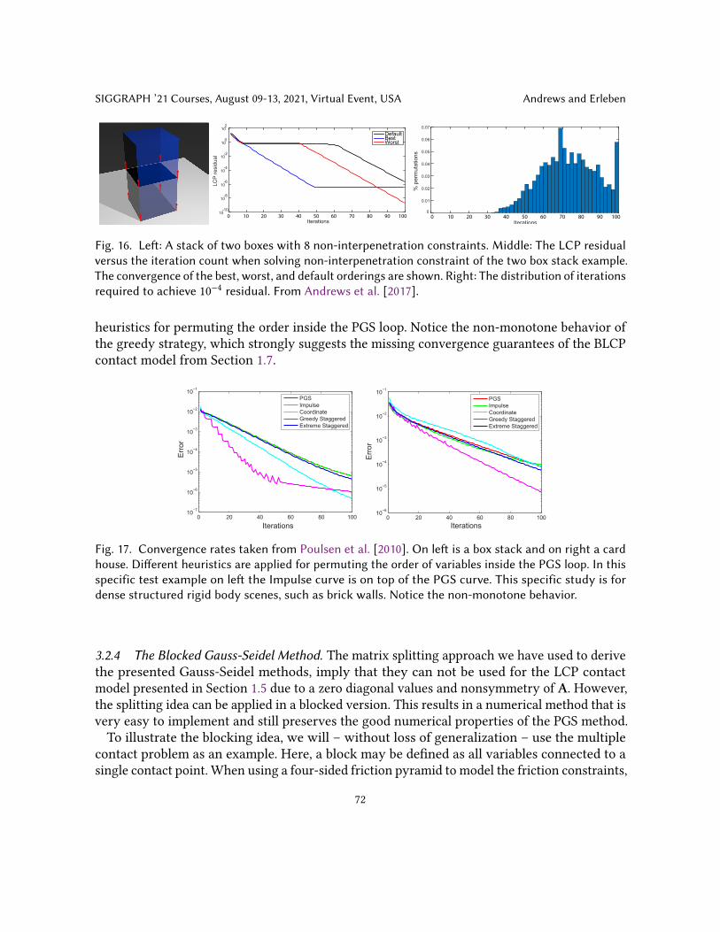
SIGGRAPH ’21 Courses, August 09-13, 2021, Virtual Event, USA Andrews and Erleben
IterationsLC
P re
sidu
al10
-10
10-8
10-6
10-4
10-2
100
102
DefaultBestWorst
0 10 20 30 40 50 60 70 80 90 100Iterations
% p
erm
utat
ions
0
0.01
0.02
0.03
0.04
0.05
0.06
0.07
0 10 20 30 40 50 60 70 80 90 100
Fig. 16. Left: A stack of two boxes with 8 non-interpenetration constraints. Middle: The LCP residualversus the iteration count when solving non-interpenetration constraint of the two box stack example.The convergence of the best, worst, and default orderings are shown. Right: The distribution of iterationsrequired to achieve 10−4 residual. From Andrews et al. [2017].
heuristics for permuting the order inside the PGS loop. Notice the non-monotone behavior ofthe greedy strategy, which strongly suggests the missing convergence guarantees of the BLCPcontact model from Section 1.7.
0 20 40 60 80 10010−7
10−6
10−5
10−4
10−3
10−2
10−1
Iterations
Erro
r
PGSImpulseCoordinateGreedy StaggeredExtreme Staggered
0 20 40 60 80 10010−6
10−5
10−4
10−3
10−2
10−1
Iterations
Erro
r
PGSImpulseCoordinateGreedy StaggeredExtreme Staggered
Fig. 17. Convergence rates taken from Poulsen et al. [2010]. On left is a box stack and on right a cardhouse. Different heuristics are applied for permuting the order of variables inside the PGS loop. In thisspecific test example on left the Impulse curve is on top of the PGS curve. This specific study is fordense structured rigid body scenes, such as brick walls. Notice the non-monotone behavior.
3.2.4 The Blocked Gauss-Seidel Method. The matrix splitting approach we have used to derivethe presented Gauss-Seidel methods, imply that they can not be used for the LCP contactmodel presented in Section 1.5 due to a zero diagonal values and nonsymmetry of A. However,the splitting idea can be applied in a blocked version. This results in a numerical method that isvery easy to implement and still preserves the good numerical properties of the PGS method.To illustrate the blocking idea, we will – without loss of generalization – use the multiple
contact problem as an example. Here, a block may be defined as all variables connected to asingle contact point. When using a four-sided friction pyramid to model the friction constraints,
72
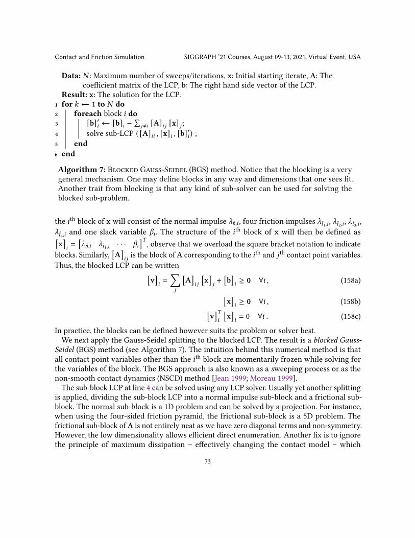
Contact and Friction Simulation SIGGRAPH ’21 Courses, August 09-13, 2021, Virtual Event, USA
Data: 𝑁 : Maximum number of sweeps/iterations, x: Initial starting iterate, A: Thecoefficient matrix of the LCP, b: The right hand side vector of the LCP.
Result: x: The solution for the LCP.1 for 𝑘 ← 1 to 𝑁 do2 foreach block 𝑖 do3 [b]′𝑖 ← [b]𝑖 −
∑𝑗≠𝑖 [A]𝑖 𝑗 [x] 𝑗 ;
4 solve sub-LCP ( [A]𝑖𝑖 , [x]𝑖 , [b]′𝑖) ;5 end6 end
Algorithm 7: Blocked Gauss-Seidel (BGS) method. Notice that the blocking is a verygeneral mechanism. One may define blocks in any way and dimensions that one sees fit.Another trait from blocking is that any kind of sub-solver can be used for solving theblocked sub-problem.
the 𝑖th block of x will consist of the normal impulse _�̂�,𝑖 , four friction impulses _𝑡1,𝑖 , _𝑡2,𝑖 , _𝑡3,𝑖 ,_𝑡4,𝑖 and one slack variable 𝛽𝑖 . The structure of the 𝑖th block of x will then be defined as[x]𝑖=
[_�̂�,𝑖 _𝑡1,𝑖 · · · 𝛽𝑖
]𝑇 , observe that we overload the square bracket notation to indicateblocks. Similarly,
[A]𝑖 𝑗is the block of A corresponding to the 𝑖th and 𝑗 th contact point variables.
Thus, the blocked LCP can be written[v]𝑖=
∑︁𝑗
[A]𝑖 𝑗
[x]𝑗+
[b]𝑖≥ 0 ∀𝑖 , (158a)[
x]𝑖≥ 0 ∀𝑖 , (158b)[
v]𝑇𝑖
[x]𝑖= 0 ∀𝑖 . (158c)
In practice, the blocks can be defined however suits the problem or solver best.We next apply the Gauss-Seidel splitting to the blocked LCP. The result is a blocked Gauss-
Seidel (BGS) method (see Algorithm 7). The intuition behind this numerical method is thatall contact point variables other than the 𝑖th block are momentarily frozen while solving forthe variables of the block. The BGS approach is also known as a sweeping process or as thenon-smooth contact dynamics (NSCD) method [Jean 1999; Moreau 1999].The sub-block LCP at line 4 can be solved using any LCP solver. Usually yet another splitting
is applied, dividing the sub-block LCP into a normal impulse sub-block and a frictional sub-block. The normal sub-block is a 1D problem and can be solved by a projection. For instance,when using the four-sided friction pyramid, the frictional sub-block is a 5D problem. Thefrictional sub-block of A is not entirely neat as we have zero diagonal terms and non-symmetry.However, the low dimensionality allows efficient direct enumeration. Another fix is to ignorethe principle of maximum dissipation – effectively changing the contact model – which
73
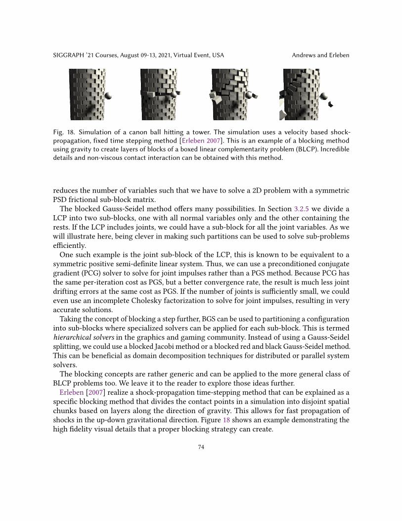
SIGGRAPH ’21 Courses, August 09-13, 2021, Virtual Event, USA Andrews and Erleben
Fig. 18. Simulation of a canon ball hitting a tower. The simulation uses a velocity based shock-propagation, fixed time stepping method [Erleben 2007]. This is an example of a blocking methodusing gravity to create layers of blocks of a boxed linear complementarity problem (BLCP). Incredibledetails and non-viscous contact interaction can be obtained with this method.
reduces the number of variables such that we have to solve a 2D problem with a symmetricPSD frictional sub-block matrix.The blocked Gauss-Seidel method offers many possibilities. In Section 3.2.5 we divide a
LCP into two sub-blocks, one with all normal variables only and the other containing therests. If the LCP includes joints, we could have a sub-block for all the joint variables. As wewill illustrate here, being clever in making such partitions can be used to solve sub-problemsefficiently.One such example is the joint sub-block of the LCP, this is known to be equivalent to a
symmetric positive semi-definite linear system. Thus, we can use a preconditioned conjugategradient (PCG) solver to solve for joint impulses rather than a PGS method. Because PCG hasthe same per-iteration cost as PGS, but a better convergence rate, the result is much less jointdrifting errors at the same cost as PGS. If the number of joints is sufficiently small, we couldeven use an incomplete Cholesky factorization to solve for joint impulses, resulting in veryaccurate solutions.Taking the concept of blocking a step further, BGS can be used to partitioning a configuration
into sub-blocks where specialized solvers can be applied for each sub-block. This is termedhierarchical solvers in the graphics and gaming community. Instead of using a Gauss-Seidelsplitting, we could use a blocked Jacobi method or a blocked red and black Gauss-Seidel method.This can be beneficial as domain decomposition techniques for distributed or parallel systemsolvers.The blocking concepts are rather generic and can be applied to the more general class of
BLCP problems too. We leave it to the reader to explore those ideas further.Erleben [2007] realize a shock-propagation time-stepping method that can be explained as a
specific blocking method that divides the contact points in a simulation into disjoint spatialchunks based on layers along the direction of gravity. This allows for fast propagation ofshocks in the up-down gravitational direction. Figure 18 shows an example demonstrating thehigh fidelity visual details that a proper blocking strategy can create.
74

Contact and Friction Simulation SIGGRAPH ’21 Courses, August 09-13, 2021, Virtual Event, USA
Fig. 19. Simulations of wall and a tower using a blocked Projected Gauss-Seidel (PGS) type of methodfor boxed linear complementarity problem (BLCP) with variable lower and upper bounds [Erleben2005].
Erleben [2005] uses a blocked PGS for a BLCP type of problem with variable lower and upperbounds. Figure 19 shows simulation results obtained with this method and Figure 20 illustratestypical convergence rates obtained during a single time-step. Notice that for these specificsimulations, the method still obtains a linear convergence rate, although the convergenceconstant varies a lot across simulations.
0 50 100 150 200 250 3000
0.05
0.1
0.15
0.2
0.25
0.3
0.35
0.4
0.45
iterations
θ(λ
i)
Box StackBall GridWallTower
(a) Convergence
0 50 100 150 200 250 30010
−30
10−25
10−20
10−15
10−10
10−5
100
iterations
log
(θ(λ
i))
Box StackBall GridWallTower
(b) Log Convergence
Fig. 20. Convergence rate plots of a single time-step for each of the configurations shown in Figure 19.
75

SIGGRAPH ’21 Courses, August 09-13, 2021, Virtual Event, USA Andrews and Erleben
3.2.5 Staggering. We will now combine the ideas of splitting the LCP and using QP reformu-lations. This is collectively referred to as staggering [Kaufman et al. 2008; Lötstedt 1984]. Weillustrate the idea for a multiple contact problem. We partition the LCP variables into threeindex sets: one corresponding to normal impulses N , one to friction impulses F , and the lastone is slack variables 𝛽 . Applying our partition would require us to solve the two coupledLCPs,
0 ≤ ANNxN + (bN + ANF xF ) ⊥ xN ≥ 0 (159)and
0 ≤[AFF e−e𝑇 0
] [xF𝛽
]+
[bF + AFNxN
`x𝑁
]⊥
[xF𝛽
]≥ 0 . (160)
In a staggered approach, we first solve the normal force LCP and then the friction force LCP.This is repeated iteratively until a fixed-point is reached. This is in essence a specialized blockedGauss-Seidel splitting method.Using the splitting of Equation 159 and Equation 160, we note that the normal force problem
has a symmetric positive semi-definite coefficient matrix ANN making QP reformulationspossible, whereas the frictional problem has an non-symmetric matrix. However, because thefriction LCP is equivalent to the first order optimality conditions of the QP problem
x∗F = arg min12x𝑇FAFF xF + c
𝑇F xF (161)
subject toxF ≥ 0 and 𝑐N − e𝑇xF ≥ 0 , (162)
where 𝑐N = `xN and cF = bF + BFNxN , any convex QP method can be used to solve for thenormal and friction forces. Thus, we are guaranteed to find a solution for each sub-problem.Whether the sequence of QP sub-problems converge to a fixed point is not obvious. Thereexist many variations over this staggering scheme [Lacoursiere and Linde 2011].Silcowitz et al. [2009] apply a kind of semi-staggering method for BLCPs. They found that
using this simple semi-staggering approach to warm start a Newton method shows howdramatically staggering can affect the convergence behavior.
3.2.6 The Projected Gauss-Seidel Subspace Minimization Method. We extend the general PGSmethod, by tailoring it to the generalized boxed LCP problem class which allows for variablelower and upper bounds. The method we derive originates from work on solving the contactforce problem [Silcowitz et al. 2010b]. The projected Gauss-Seidel with Subspace Minimization(PGS-SM) method is an iterative method, and each iteration consists of two phases:(1) The first phase estimates a set of active constraints F using the standard PGS method.(2) The second phase solves accurately for the active constraints, potentially further reducing
F for the next iteration.Phase I. This phase consists of running a standard PGS method to solve for x. When the PGS
algorithm terminates, we know that x is feasible, although not necessarily the correct solution.
76

Contact and Friction Simulation SIGGRAPH ’21 Courses, August 09-13, 2021, Virtual Event, USA
However, v may be infeasible due to the projection on x made by the PGS method. Recall thedefinitions given by Equation 110a-110c, which are practical for labeling and eliminating someof the unknowns based on analysis of the feasibility and complementarity conditions. In fact,the pivoting based solver exploited this aspect of the index set definitions. A similar approachis taken by the second phase of the PGS-SM method, which solves for a a subset of variables.Phase II. The linear system may be partitioned as in Equation 109 into three distinct sets:
free and tight lower and upper bounded. To solve this system for the unknowns vL, vU and xF,we first compute xF by solving
AF,FxF = −(bF + AF,L𝝀
loL + AF,U𝝀
hiU
). (163)
Here, AF,F is a symmetric principal sub-matrix of A. Knowing xF, we can easily compute vLand vU,
vL = ALFxF + ALL𝝀loL + ALU𝝀
hiU + bL, (164a)
vU = AUFxF + AUL𝝀loL + AUU𝝀
hiU + bU. (164b)
Now, we check that the feasibility conditions are satisfied: vL < 0, vU > 0 and 𝝀loF ≤ xF ≤ 𝝀hi
F.If all constraints are satisfied, we have reached a solution. Rather than testing the constraintsexplicitly, a projection is performed on the reduced problem:
xF ← min(xhiF ,max(xloF , xF)) . (165)
We assemble the full solution vector x←[x𝑇F l𝑇L u𝑇U
]𝑇 before re-estimating the index setsfor the next iteration. The projection on the reduced problem will either leave the activeset unchanged or reduce it further. See Algorithm 8 for the full pseudo code of the PGS-SMmethod.Notice that Algorithm 8 does not specify which termination criteria to use . A particularly
useful termination criterion for the PGS-SM method could be to monitor if the set F haschanged from the previous iteration,
F𝑘+1 = F𝑘 . (166)
Figure 21 shows different simulation results obtained with the PGS-SM method [Silcowitzet al. 2010b]. As shown the PGS-SM method behaves rather well for small configurations andconfigurations with joints. For larger configurations, we obtain convergence results similar tothe PGS method.
3.2.7 The Non-Smooth Nonlinear Conjugate Gradient Method. Silcowitz et al. [2010a] showsthat the PGS iteration can be written in generic form using Equation 156 as
x𝑘+1 = min( u(x𝑘)︸︷︷︸T𝑈 x𝑘+t𝑈
,max( l(x𝑘)︸︷︷︸T𝐿x𝑘+t𝐿
,−(D + L)−1(Ux𝑘 + b︸ ︷︷ ︸Tx𝑘+t
)) (167)
77

SIGGRAPH ’21 Courses, August 09-13, 2021, Virtual Event, USA Andrews and Erleben
Data: 𝑘𝑝𝑔𝑠 : Number of PGS sweeps per outer iteration, 𝑘𝑠𝑚: Number of subspace solvesper outer iteration, x: The initial iterate, A: The coefficient matrix of the BLCP, b:The right hand side vector the BLCP.
Result: x: The numerical solution for the BLCP.1 while not converged do2 x← run PGS for at least 𝑘𝑝𝑔𝑠 iterations;3 if termination criteria reached then4 return x;5 end6 for 𝑘 ← 1 to 𝑘𝑠𝑚 do7 L ≡ {𝑖 |x𝑖 = l𝑖};8 U ≡ {𝑖 |x𝑖 = u𝑖};9 F ≡ {𝑖 |l𝑖 < x𝑖 < u𝑖};
10 solve: AF,FxF = −(bF + AF,LlL + AF,UuU
);
11 vL ← AL,FxF + AL,LlL + AL,UuU + bL;12 vU ← AU,FxF + AU,LlL + AU,UuU + bU;13 update: (l, u);14 xF ← min(uF,max(lF, xF));15 x←
[x𝑇F l𝑇L u𝑇U
]𝑇 ;16 if termination criteria reached then17 return x18 end19 end20 end
Algorithm 8: Projected Gauss-Seidel subspace minimization (PGS-SM) method.Observe that is can be seen as a PGS solver followed by an active-set strategy solving asequence of linear systems while efficiently updating the active index set. PGS becomes aprior for making a good initial estimate of the active set.
where the lower and upper bound functions l, u : R𝑛 ↦→ R𝑛 are affine functions. The T𝐿 and T𝑈matrices express the linear relations between the tangential friction forces and their associatednormal forces. The t𝐿 and t𝑈 vectors can be used to express fixed bound constraints, such asa normal force constraint. Thus, the PGS iteration can be perceived as a selector function ofthree affine functions.
78

Contact and Friction Simulation SIGGRAPH ’21 Courses, August 09-13, 2021, Virtual Event, USA
0 500 1000 150010
−40
10−20
100
1020
Arched Snake
PGS iterations
Ψ(λ
k )
PGS−SMPGS
(a)
0 500 1000 150010
−10
10−5
100
105
Heavy Box On Arched Snake
PGS iterations
Ψ(λ
k )
PGS−SMPGS
(b)
0 500 1000 150010
−20
10−10
100
1010
Large Stack of Boxes
PGS iterations
Ψ(λ
k )
PGS−SMPGS
(c)
0 500 1000 150010
−20
10−10
100
1010Heavy Box Resting On Light Boxes
PGS iterations
Ψ(λ
k )
PGS−SMPGS
(d)
0 500 1000 150010
−10
10−5
100
105Boxes Resting On Inclined Surface
PGS iterations
Ψ(λ
k )
PGS−SMPGS
(e)
0 500 1000 150010
−10
10−5
100
105
Small Pyramid of Gears
PGS iterations
Ψ(λ
k )
PGS−SMPGS
(f)
0 500 1000 150010
−10
10−5
100
105
Medium Pyramid Of Gears
PGS iterations
Ψ(λ
k )
PGS−SMPGS
(g)
0 500 1000 150010
−5
100
105
Friction Dependant Structure
PGS iterations
Ψ(λ
k )
PGS−SMPGS
(h)
Fig. 21. Test cases for the comparison of PGS and PGS–SM methods with corresponding convergenceplots. Observe the jaggedness in the PGS–SM plots in (b), (c), (d), and (g). The spikes indicates that thePGS–SM method guessed a wrong active set. This can cause the merit function to rise abruptly. The𝜓 function is the Fischer–Burmeister function from Silcowitz et al. [2009]. The 𝑥-axis is measured inunits of one PGS iteration to make comparison easier.
Assuming a converging sequence x𝑘 → x∗ for 𝑘 →∞ the solution of PGS can be written asthe fixed point formulation,
x∗ = min(T𝑈 x∗ + t𝑈 ,max(T𝐿x∗ + t𝐿,Tx∗ + t))︸ ︷︷ ︸≃Gx∗+g
. (168)
The right hand side of Equation 168 can be conceptually considered as the evaluation of anaffine function, Gx∗ + g. This is true if the active set of constraints is known in advance.Therefore, we have
0 = (G − I)x∗ + g . (169)
Observe, explicit assembly is not needed for any of the matrices, instead the PGS method canbe used to implicitly evaluate the residual of any given iteration, r𝑘 = (G − I)x𝑘 + g. Thus, ifwe write one iteration of the standard PGS method as
x𝑘+1 = PGS(x𝑘) (170)
then r𝑘 = x𝑘+1 − x𝑘 = PGS(𝑥𝑘) − x𝑘 . This can be thought of as the gradient of a non-smooth nonlinear quasi-quadratic function 𝑓 (x𝑘) ≈ 1
2 ∥r𝑘 ∥2. We are essentially seeking a
79

SIGGRAPH ’21 Courses, August 09-13, 2021, Virtual Event, USA Andrews and Erleben
local minimizer of 𝑓 , however, we only know its gradient ∇𝑓 (x𝑘) = r𝑘 . The Fletcher-Reevesnonlinear conjugate gradient method is perfect for this [Nocedal and Wright 2006].In each iteration of the conjugate gradient method we perform the update,
x𝑘+1 = x𝑘 + 𝜏𝑘p𝑘 (171)
where p𝑘 is the search direction and 𝜏𝑘 can be found using a line search method. Next a newsearch direction is computed by
𝛽𝑘+1 =
∇𝑓 𝑘+1 2 ∇𝑓 𝑘 2 , (172a)
p𝑘+1 = 𝛽𝑘+1p𝑘 − ∇𝑓 𝑘+1 . (172b)
In an an interactive context, the line search on 𝑓 (x𝑘+1) is dropped. Here the full step length,𝜏 = 1, is used and the method is restarted whenever ∥∇𝑓 𝑘+1∥2 > ∥∇𝑓 𝑘 ∥2.When computing PGS(x𝑘), it is practical to do so in-place, meaning that a PGS step is taken
implicitly on x𝑘 . Therefore, the update of x𝑘 is done separately in two places in each iteration.The full algorithm is stated in Algorithm 9.An implementation of the non-smooth nonlinear conjugate gradient (NNCG) method can be
found in [Silcowitz-Hansen 2010] and [Coumans 2005]. Detailed convergence studys may befound in [Silcowitz et al. 2010a]. Figure 22 shows corresponding convergence rates for somesimulation results, taken from [Silcowitz et al. 2010a]. Figure 22 Notice the dramatic change inconvergence behavior. The improved accuracy means the NNCG method is more equipped todeal with for instance large mass ratios. Usually PGS performs slow on such problems andNNCG will out-perform it. Further, NNCG is overall computationally cheaper than applying adirect method which otherwise would be able to handle large mass ratios.
3.3 Non-Smooth Newton MethodsLet us just remember the classical Newton method for solving a generic roots search problemF(x) = 0, that is solve for x such that the vector function F is zero. The Newton method isclassically derived from a first order Taylor approximation around the 𝑘 th iterate,
F(x𝑘 + Δx) ≈ F(x𝑘) + 𝜕F(x𝑘)
𝜕xΔx . (173)
Setting the approximation equal to zero we have the Newton equation,
𝜕F(x𝑘)𝜕x
Δx = −F(x𝑘) . (174)
The Δx is called the search direction or Newton direction. We solve the Newton equation forfinding the search direction. The search direction is then used in the Newton update rule given
80

Contact and Friction Simulation SIGGRAPH ’21 Courses, August 09-13, 2021, Virtual Event, USA
Data: x: The initial iterate, A: The coefficient matrix of the LCP , b: The right hand sideof the LCP.
Result: x: The numerical solution for the LCP.1 x1 ← PGS(x0);2 ∇𝑓 0 ← −(x1 − x0);3 p0 ← −∇𝑓 0;4 𝑘 ← 1;5 while not converged do6 x𝑘+1 ← PGS(x𝑘);7 ∇𝑓 𝑘 ← −(x𝑘+1 − x𝑘);8 𝛽𝑘 ←
∇𝑓 𝑘 2/ ∇𝑓 𝑘−1
2;9 if 𝛽𝑘 > 1 then10 p𝑘 ← 0 ; /* restart */11 else12 x𝑘+1 ← x𝑘+1 + 𝛽𝑘p𝑘−1;13 p𝑘 ← 𝛽𝑘p𝑘−1 − ∇𝑓 𝑘 ;14 end15 𝑘 ← 𝑘 + 1;16 end
Algorithm 9: Nonsmooth nonlinear conjugate gradient (NNCG) method. Observehow a single PGS sweep is used to compute the gradient ∇𝑓 of some imaginary objectivefunction 𝑓 that NNCG method tries to minimize. It is surprisingly that we do not need tobe able to explicitly create 𝑓 .
by,x𝑘+1 = x𝑘 + Δx . (175)
The Newton method can be globalized by adding a line-search method to the update rule.This essentially consist of multiplying the search direction by a scalar line-step parameter.Line-search strategies are sometimes avoided in interactive and real-time simulations as theycan be expensive, but back-tracking strategies are quite popular when a line-search is added. Inthese notes we will not go into line-search methods, but instead focus on how to reformulatethe contact and friction problem into a root search problem. In the text below we will startby building up the mathematical parts that allow us to define a F-function in the context ofcontact problems and provide the building blocks for later showing how to assemble 𝜕F(x𝑘 )
𝜕xand solve for Δx.One successful approach by Ferris and Munson [1999] is to reformulate a complementar-
ity problem in terms of a NCP function whose roots satisfy the original complementarity
81

SIGGRAPH ’21 Courses, August 09-13, 2021, Virtual Event, USA Andrews and Erleben
(a) (b) (c)
(d) (e) (f)
(g) (h) (i)
Fig. 22. Test results comparing the nonlinear conjugate gradient method (NNCG) with projectedGauss-Seidel (PGS) method with up to 5000 iterations. The NNCG method clearly converges faster,and often to a higher accuracy than that of the PGS method. Notice the superior rate of convergencein (f)-(i).
conditions. In other words, functions where the following equivalence holds:
𝜓 (𝑎, 𝑏) = 0 ⇐⇒ 0 ≤ 𝑎 ⊥ 𝑏 ≥ 0 . (176)
82

Contact and Friction Simulation SIGGRAPH ’21 Courses, August 09-13, 2021, Virtual Event, USA
Combined with an appropriate time-discretization, such a NCP function turns our contactproblem into a root finding one. In general the functions𝜓 are non-smooth, but allow us toapply a wide range of numerical root finding methods [Munson et al. 2001].Let us review some of the most commonly used NCP functions and show how to rephrase
the contact problem into an equivalent root search problem.
3.3.1 Minimum-Map Formulation. The first NCP function we will consider is the minimum-map defined as
𝜓mm(𝑎, 𝑏) ≡ min(𝑎, 𝑏). (177)
The equivalence of this function to the original NCP can be verified by examining the valuesassociated with each conditional case for finding a root for the equation 𝜓mm = 0. Wenow consider how this reformulation applies to unilateral contact constraints. Recall thatthe complementarity condition associated with a contact constraint 𝜙 (q) and its associatedLagrange multiplier _�̂� is
0 ≤ 𝜙 (q) ⊥ _�̂� ≥ 0 . (178)
We can write this in the equivalent minimum-map form of the contact constraint as
𝜓�̂� (q, _�̂�) ≡ 𝜓mm(𝜙 (q), _�̂�) = 0 , (179)
which has the following derivatives,
𝜕𝜓�̂�
𝜕q=
{∇𝜙 (q), 𝜙 (q) ≤ _�̂�0, otherwise
, (180)
𝜕𝜓�̂�
𝜕_�̂�=
{0, 𝜙 (q) ≤ _�̂�1, otherwise
. (181)
From these cases we can see that the minimum-map gives rise to an active-set style methodwhere a contact is considered active if 𝜙 (q) ≤ _�̂� . Active contacts are treated as equalityconstraints, while for inactive contacts the minimum-map enforces that the constraint’sLagrange multiplier is zero.
3.3.2 Fischer-Burmeister Formulation. An alternative NCP function is given by Fischer [1992],who observe the roots of the following equation satisfy complementarity:
𝜓 fb(𝑎, 𝑏) = 𝑎 + 𝑏 −√𝑎2 + 𝑏2 = 0 . (182)
This is the Fischer-Burmeister function, and it is interesting because, unlike the minimum-map,it is smooth everywhere apart from the point (𝑎, 𝑏) = (0, 0). For (𝑎, 𝑏) ≠ (0, 0) the partial
83

SIGGRAPH ’21 Courses, August 09-13, 2021, Virtual Event, USA Andrews and Erleben
derivatives of the Fisher-Burmeister function are given by:
𝛼 (𝑎, 𝑏) = 𝜕𝜓 fb
𝜕𝑎= 1 − 𝑎
√𝑎2 + 𝑏2
, (183)
𝛽 (𝑎, 𝑏) = 𝜕𝜓 fb
𝜕𝑏= 1 − 𝑏
√𝑎2 + 𝑏2
. (184)
At the point (𝑎, 𝑏) = (0, 0) the derivative is set-valued. For Newton methods it suffices tochoose any value from this sub-gradient. Erleben et al. [2011] compared how the choice ofderivative at the non-smooth point affects convergence for LCP problems and found no overallbest strategy. Thus, for simplicity we make the arbitrary choice of
𝛼 (0, 0) = 0 , (185)𝛽 (0, 0) = 1 . (186)
For a contact constraint𝜙 , with Lagrangemultiplier _�̂� wemay thenwrite our contact constraintalternatively as,
𝜓�̂� (q, _�̂�) ≡ 𝜓 fb(𝜙 (q), _�̂�) = 0 , (187)
with derivatives given by
𝜕𝜓�̂�
𝜕q= 𝛼 (𝜙, _�̂�)∇𝜙 , (188)
𝜕𝜓�̂�
𝜕_�̂�= 𝛽 (𝜙, _�̂�) . (189)
3.3.3 Friction. Coulomb’s law can be derived from a principle of maximal dissipation thatrequires the frictional forces remove the maximum amount of energy from the system whilehaving their magnitude bounded by the normal force:
arg min𝝀𝑡
v𝑡𝑇𝝀𝑡 subject to ∥𝝀𝑡 ∥ ≤ `_�̂� . (190)
This minimization defines an admissible cone that the total contact force must lie in. TheLagrangian associated with this minimization is
L(𝝀𝑡 , _�̂�) ≡ v𝑡𝑇𝝀𝑡 + 𝛾 (∥𝝀𝑡 ∥ − `_�̂�) . (191)
where 𝛾 is a slack variable used to enforce the Coulomb constraint that the friction forcemagnitude is bounded by ` times the normal force magnitude. When `_�̂� > 0 the problemsatisfies Slater’s condition [Boyd and Vandenberghe 2004] and we can use the first-order
84

Contact and Friction Simulation SIGGRAPH ’21 Courses, August 09-13, 2021, Virtual Event, USA
Karush-Kuhn-Tucker (KKT) conditions, given by
s(u,𝝀𝑡 , 𝛾) ≡ J𝑡u + 𝛾𝜕∥𝝀𝑡 ∥𝜕𝝀𝑡
= 0 (192)
0 ≤ 𝛾 ⊥ `_�̂� − ∥𝝀𝑡 ∥| ≥ 0 , (193)
where 𝛾 is a slack variable that governs stick/slip behavior, and we used the block notation forthe mapping v = Ju given by
v =
[𝑣�̂�v𝑡
]=
[J�̂�J𝑡
]︸︷︷︸
J
u . (194)
The complementarity condition may be directly written using any NCP function as,
𝜓𝑡 ≡ 𝜓 (𝛾, `_�̂� − ∥𝝀𝑡 ∥) = 0 . (195)
3.3.4 Newton’s Method. We may now define generically for any chosen NCP function,
x ≡
u_�̂�𝝀𝑡𝛾
and F(x) ≡
Mu − J𝑇_ + f𝜓�̂� (𝜙 (q), _�̂�)s(u,𝝀𝑡 , 𝛾)
𝜓𝑡 (𝛾, `_�̂� − ∥𝝀𝑡 ∥)
= 0 , (196)
Observe the top-row in F is the time-discretized Newton Euler equations. One may replacethe normal reformulation with one that is based on the separation velocity 𝑣�̂� rather than thenormal constraint 𝜙 . In which case we have𝜓�̂� ( ¤𝜙, _�̂�) = 𝜓�̂� (𝑣�̂�, _�̂�) = 𝜓�̂� (J�̂� u, _�̂�). We can solvefor the roots of𝜓�̂� and𝜓𝑡 using Newton’s methods by linearizing the equation F = 0 in termsof velocities and the Lagrange multipliers to obtain the following system,
M −J�̂�𝑇 −J𝑡𝑇 0J�̂�
𝜕𝜓�̂�𝜕_�̂�
0 0J𝑡 0 𝜕s
𝜕𝝀𝑡
𝜕s𝜕𝛾
0 𝜕𝜓𝑡𝜕_�̂�
𝜕𝜓𝑡𝜕𝝀𝑡
𝜕𝜓𝑡𝜕𝛾
ΔuΔ_�̂�Δ𝝀𝑡Δ𝛾
= −
f𝜓�̂�s𝜓𝑡
. (197)
Here we have considered a single contact constraint for simplicity. The extension to a systemof contacts is straightforward. However, it is clear that, due to the frictional constraints,Equation 197 is non-symmetric, which restricts the numerical methods we can use to solve it.Macklin et al. [2019] proposed a fixed-point iteration to eliminate 𝛽 and obtain a symmetricsystem that can be solved with iterative Krylov methods.
3.3.5 Preconditioning. Similar to prox formulations, the NCP functions presented in thissection have a free parameter 𝑟 that may be used to rescale the functions. Specifically, asolution to𝜓 (𝑎, 𝑏) = 0, is also a solution to the scaled problem,𝜓 (𝑎, 𝑟𝑏) = 0, where 𝑟 may be
85

SIGGRAPH ’21 Courses, August 09-13, 2021, Virtual Event, USA Andrews and Erleben
-1 -0.5 0 0.5 1-1
-0.5
0
0.5
1r=1
rc( )min(c, r )fb(c, r )
-1 -0.5 0 0.5 1-1
-0.5
0
0.5
1r=0.25
rc( )min(c, r )fb(c, r )
Fig. 23. Left: The minimum-map of a unilateral constraint has a kink in it at the cross over point. Right:Choosing an appropriate r-factor can remove the discontinuity by forcing both terms to be parallel. Fora single constraint this results in a straight-line error function that can be solved in one step regardlessof starting point. In the case of Fischer-Burmeister (green) the error function’s curvature is reduced.For illustration purposes we have shown the constraint function 𝑐 = 1
4_ −18 > 0, which has a unique
solution at _ = 12 .
chosen as any positive constant. In practice this parameter is important for the robustness ofNewton methods, and we visualize its effect on the NCP functions in Figure 23.
86

Contact and Friction Simulation SIGGRAPH ’21 Courses, August 09-13, 2021, Virtual Event, USA
4 SELECTED TOPICSWe will now look a little on topics that goes beyond what could be considered the classicalfundamental syllabus of contact and friction simulation.We have chosen to cover the topic of proximal operators as these are a quite general and
powerful framework for expression the contact physics as well as with ease provide a simpleway to derive numerical methods. Our treatment is extensive and show many facets of how touse proximal operators in a simulator.Following the treatment of proximal operators we dive into more advanced friction modeling.
We present a recent model that originated from the field of computer graphics which canaccount for anisotropic friction effects. The model is named Matchstick model and it fitsbeautifully into the framework of the proximal operators and as such we feel it is a good fit forshowing the need for more general formulations, while at the same time underlining currentstate-of-the-art models that try to move beyond limitations of isotropic Coulomb friction law.The last topic we cover in this section is on presenting one large and fundamentally different
alternative to the constraint based methods which we have covered extensively in previouschapters. The topic is penalty-based methods for contact modeling. We have selected to coverthis topic to provide a broader and more complete coverage of the subject of contact andfriction simulation. Besides the penalty-based and constraint-based approaches are sometimecombined in actual implementations into "hybrid" simulators. This is evident from the strongconnection between constraint stabilisation and penalty-based methods.
4.1 Proximal OperatorsIterative methods are popular for solving contact force problems in rigid body dynamics. Wehave extensively covered many of the LCP variations of these type of methods. The ideasdo extend into other types of models. One such model is based on the proximal operator. Itis a much more general model that allow one to express more nonlinear and non smoothproperties in a compact way than the LCP approach often would allow one to do. In thissection we extend many previous ideas covered in previous sections into this more generalabstract setting building on proximal operators. We provide a mathematical foundation forcomputer graphics researchers for iterative (PROX) schemes based on proximal operators. Ourpresentation follows the outline of Erleben [2017]. We derive a class of iterative Jacobi andblocked Gauss-Seidel variants that theoretically proven always converge and provides flexibleplug and play framework for exploring different friction laws as we describe in Section 4.2.PROX methods are both fast, scale to handle a large number of rigid bodies, deal with non-convex shapes, accurately model the physics, and be robust as well as predictable in case ofuser interactions as illustrated in Figure 24.The PGS type of methods have become quite a de-facto standard for interactive entertainment.
The robustness of PGS and PSOR variants are well-known as is their poor convergence behavior[Andrews et al. 2017; Erleben 2007]. We provide a derivation of such iterative schemes using
87

SIGGRAPH ’21 Courses, August 09-13, 2021, Virtual Event, USA Andrews and Erleben
Fig. 24. Examples of rigid body simulation using PROX schemes. Top row shows digital prototypingapplication studying jamming due to friction properties, upper-middle: packing into a container, middle-lower: building collapse due to poor design. Bottom demonstrates structured stacking.
proximal operators. We name these schemes PROX methods to avoid confusion with thetraditional PGS variants as described in Section 3.2. We will take a different path based onproximal operators than the usual PGS-type derivation such as the one done by Silcowitz et al.[2010a].Interestingly, the usual PGS complementarity based friction box-model variants are special
cases of a PROX method with a fixed constant 𝑟 -factor (to be explained later). This is the reasonwhy PGS can diverge and why the PROX method setting is theoretically guaranteed to alwaysconverge [Foerg et al. 2006; Parikh and Boyd 2014]. Further, PGS is tied to the box-model forperformance reasons as it provides a small tight blocked memory footprint. PROX methods arein their very derivation not limited to such friction models. PROX schemes provide one withboth a theoretical guarantee of convergence and a flexible modeling of any convex multi-setfriction law. For completeness we show the model can express Newton style impact laws, andpost-stabilization. The proximal operator model is derived directly from physical principlesand is in our opinion a very powerful approach. One benefit is that the iterative scheme forcomputing a solution more or less comes for free directly from the model it self. No extradiscretization are needed. Another benefit of this model is that it generalizes to general limitsurfaces [Goyal et al. 1989] and can include torsional friction and Coulomb friction [Leine andGlocker 2003].
88

Contact and Friction Simulation SIGGRAPH ’21 Courses, August 09-13, 2021, Virtual Event, USA
Fig. 25. The proximal operator for a set C applied to a point z. Observe that computing a solution x★
for the proximal operator is similar to point in set testing and projection to closest point on a boundary.The set C can have a non-smooth boundary.
4.1.1 The Proximal Operator Model. We will present a contact force model for a single contactpoint. The notation makes use of a proximal operator, proxC (z). The proximal point of aconvex set C to a point z is the point in C that minimizes the distance to z,
proxC (z) ≡ arg minx∈𝐶
∥z − x∥2 , z ∈ R𝑛 . (198)
this is called the proximal operator [Parikh and Boyd 2014]. This definition is illustrated inFigure 25. For friction modeling we usually only require C to be convex. Notice that C is strictconvex then the solution is always unique. The weaker requirement of only being convex canimply multiple solutions. One advantage of this formulation is that we can work with a C thathas a non-smooth boundary. That is the normal cone at a boundary point has a sub-space ofnormals. The requirement for C to be convex is one of the ingredients connected to givingstrong guarantee that a fixed point scheme will converge. The proximal operator definitioncan be weaken to give meaning for non-convex sets too. We do not go into this discussion inthis text.Given the normal contact velocity 𝑣�̂� ∈ R then the non-penetration constraints can be stated
as𝑣�̂� ≥ 0, _�̂� ≥ 0, and 𝑣�̂�_�̂� = 0 , (199)
or equivalently the fixed point relationship have the same solution as the non-penetrationconstraint [Jourdan et al. 1998]
_�̂� = proxN (_�̂� − 𝑟�̂�𝑣�̂�) for 𝑟�̂� > 0 , (200)where N ≡ {𝛾 ∈ R | 𝛾 ≥ 0}, _n̂ ∈ R is the magnitude of the normal force, and 𝑟�̂� is amathematical scalar variable named an 𝑟 -factor, we use the subscript here to denote thatthe value is specific for the normal force as we will see later friction forces can have their own
89

SIGGRAPH ’21 Courses, August 09-13, 2021, Virtual Event, USA Andrews and Erleben
(a) (b)
Fig. 26. In (a) we observe that if the normal force is positive then the proximal operator only has afixed point if the normal velocity is zero. In (b) the case of zero normal shows that a fixed point onlyexist if the normal velocity is non-negative. This proves the fixed point formulation with the proximaloperator has the same solutions as the non-penetration constraint.
𝑟 -factor value. The equation holds for all 𝑟�̂� > 0 and the exact 𝑟 -factor value will have practicalimpact on convergence. We can graphically illustrate how the proximal operator identifies thesame solutions as the complementary form of the non-penetration constraint by using thereal number line. Here N is all numbers from origin to the right. The case-by-case analysis isshown in Figure 26.It is not difficult to show that the proximal operator formulation includes all the LCP based
formulations. For doing this it is convenient to use the slightly more general proximal operatordefinition
x★ ≡ proxKC (x − 𝑟 (Ax + b)) , K = A−1, C = {x | x ≥ 0} ∀𝑟 > 0 . (201)Let z = x − 𝑟 (Ax + b) then by more general definition of the proximal operator we have
x★ ≡ arg minx∈C
12∥x − z∥2K , (202)
which we can algebraic transform into
x★ ≡ arg minx∈C
𝑟 2 (Ax + b)𝑇 K (Ax + b) . (203)
The positive term 𝑟 2 can be dropped without affecting the solution of the minimization problemand the quadratic term can be written out to yield the equivalent problem,
x★ ≡ arg minx∈C
x𝑇A𝑇KAx + b𝑇K(A𝑇 + A
)x + b𝑇Kb . (204)
Using the explicit choice of K = A−1 and assuming A is symmetric this reduces to
x★ ≡ arg minx∈C
x𝑇Ax + 2b𝑇x (205)
90

Contact and Friction Simulation SIGGRAPH ’21 Courses, August 09-13, 2021, Virtual Event, USA
orx★ ≡ arg min
x∈C
12x𝑇Ax + b𝑇x . (206)
This happens to be the equivalent quadratic problem (QP) reformulation of the linear com-plementarity problem. This can be verified by noticing that the solution to the first orderoptimality conditions for the QP formulation is the solution to the linear complementarityproblem. This completes the proof that solutions of LCP formulations are also solutions forthe proximal operator formulations.Given the coefficient of friction ` > 0 and the magnitude of normal force _�̂� ≥ 0, then the
planar friction force 𝝀𝑡 ∈ R2 is bounded by the friction cone,
𝝀𝑡 ∈ F (`_�̂�) (207)
where the friction cone could be defined as we did in Section 1.5,
F (`_�̂�) ≡{𝜸 𝑡 ∈ R
2 �� 𝜸 𝑡 ≤ `_�̂�} . (208)
This is the typical isotropic Coulomb friction law. We will later show another example. Forthe proximal operator model to work we only need F to be a convex set. We may visualizethe friction cone in 3D where the 𝑥 and 𝑦 axis gives the components of the frictional forceand the 𝑧-axis gives the normal force magnitude as shown in Figure 27. Another often usedvisualization is to make a corresponding 2D visualization of the intersection of the cone withthe 𝑧-plane that corresponds to the current normal force as shown in middle of Figure 27.Because the friction force scales linear with normal force the shape of the 2D intersection willnot change for any positive normal force and we one may therefore just draw the shape of thecone for the normal force value _�̂� = 1. The cone-shape then illustrates the magnitude of thecoefficient of friction for different directions as seen in right side Figure 27.According to principle of maximum dissipation the friction force should dissipate as much
work as possible from the system. Given the friction force 𝝀𝑡 ∈ F (`_�̂�) and the tangentialcontact velocity, v𝑡 ∈ R2, then the dissipation power, 𝑃𝝀𝑡
, is,
𝑃𝝀𝑡= 𝝀𝑡
𝑇v𝑡 . (209)
Note that dissipation implies that 𝑃𝝀𝑡< 0. According to the principle of maximum dissipation
the power, 𝑃𝜸𝑡, done by any other possible friction force, 𝜸 𝑡 ∈ F (`_�̂�), has to be larger than or
equal to 𝑃𝝀𝑡. From this we have
𝑃𝝀𝑡≤ 𝑃𝜸𝑡
, (210a)
𝝀𝑡𝑇v𝑡 ≤ 𝜸 𝑡
𝑇v𝑡 , (210b)
0 ≤ 𝜸 𝑡𝑇v𝑡 − 𝝀𝑡𝑇v𝑡 =
(𝜸 𝑡 − 𝝀𝑡
)𝑇 v𝑡 . (210c)
Resulting in the condition
∀𝜸 𝑡 ∈ F (`_�̂�) and(𝜸 𝑡 − 𝝀𝑡
)𝑇 v𝑡 ≥ 0 . (211)
91

SIGGRAPH ’21 Courses, August 09-13, 2021, Virtual Event, USA Andrews and Erleben
Fig. 27. On the left the isotropic Coulomb friction cone is shown as an ice-cream cone, in the middlethe 2D plane intersection with the normal force plane is representing the shape of the friction set, andon the right we have a map of the set of coefficients of friction. Observe that the map of coefficients offrictions is a convenient representation of any friction cone that can be used to generate both the 2Dfriction set and the 3D friction cone if needed.
Recall, we derived this condition in Section 1.5 from first order optimality conditions, here wejust took a more direct geometric approach for deriving this condition. Now a solution to thisvariational inequality is equivalent to the fixed point of the proximal operator,
𝝀𝑡 = proxF (`_�̂�) (𝝀𝑡 − 𝑟𝑡v𝑡 ) for 𝑟𝑡 > 0 . (212)
Figure 28 illustrates how the principle of maximum dissipation is connected to the proximaloperator, by connecting the variational inequality to the definition of the tangent cone andfinally testing if −v𝑡 is included in the normal cone at 𝝀𝑡 . The tangent and normal coneviewpoint is quite helpful in handling the case of zero sliding velocity. In this case we notethat there are no dissipating forces. This means the tangent cone is all directions in the planeand the normal cone contains the zero-vector. This means that any force in the friction cone isa solution to principle of maximum dissipation. Notice that the proximal operator will havethis solution too.Since v =
[𝑣�̂�𝑇v𝑡𝑇
]𝑇 can be written as a linear combination of 𝝀 =[_�̂�𝑇 𝝀𝑡
𝑇]𝑇 we have
v = A𝝀 + b. The equation holds for all values of the variable 𝑟𝑡 but the actual value used willhave impact on convergence. Substituting v into the proximal operator lead to a fixed pointproblem, [
_�̂�𝝀𝑡
]︸︷︷︸
𝝀
=
[proxN (_�̂� − 𝑟�̂� (ANN_�̂� + ANF𝝀𝑡 + bN))
proxF (`_�̂�) (𝝀𝑡 − 𝑟𝑡 (AFN_�̂� + AFF𝝀𝑡 + bF))
]︸ ︷︷ ︸
F(𝝀)
. (213)
92

Contact and Friction Simulation SIGGRAPH ’21 Courses, August 09-13, 2021, Virtual Event, USA
(a) (b)
(c) (d)
Fig. 28. The proximal operator can be derived from the principle of maximum dissipation. We start withsome convex friction cone and assume a non-zero sliding velocity. Given the velocity vector we maylook in the whole half-space of dissipating forces (a). In this space we locate the maximum dissipatingforce as done in (b). In (c) we slightly reformulate the dissipation test to look at the force differencevectors. Any such force difference vector must make a positive dot product with the velocity. That isequivalent to saying that any direction in the tangent cone at 𝝀𝑡 must make a positive product withthe velocity. Taking this one step further that means the negative velocity must be in the normal coneat 𝝀𝑡 . That is equivalent to say that any point on the half-line from 𝝀𝑡 in the negative velocity directionmust have 𝝀𝑡 as the closest point on the surface as shown in (d).
Here N and F are index sets used to extract blocks from A corresponding to normal forcevariables or friction force variables. Now one could compute the iterates, 𝝀𝑘+1 = F(𝝀𝑘), moredetails are given in Section 4.1.2. The iteration sequence converges locally if the spectral radius
93

SIGGRAPH ’21 Courses, August 09-13, 2021, Virtual Event, USA Andrews and Erleben
of the Jacobian,
𝜌
(𝜕F(𝝀)𝜕𝝀
)< 1 , (214)
remains limited and smaller than one. This requirement can be realized by making a suitablechoice of the parameters 𝑟�̂� and 𝑟𝑡 [Foerg et al. 2006; Niebe 2014; Parikh and Boyd 2014; Studer2008].The Newton-Euler equations and kinematic maps are given by
M ¤u = f + J𝑇𝝀 , (215a)¤q = Hu , (215b)
where u is the generalized velocity vector, q is generalized position vector,M is the mass matrix,J is the contact Jacobian, and f holds external and gyroscopic force terms, see Section 1.10.1for details. The relative contact velocity is computed from
v = Ju . (216)
All the contact constraints are now formulated using proximal operators,
∀𝑖 _�̂�𝑖 = proxN𝑖
(_�̂�𝑖 − 𝑟�̂�𝑖
(𝑣�̂�+𝑖 + Y�̂�𝑖𝑣�̂�−𝑖
) ), (217a)
∀𝑖 𝝀𝑡 𝑖 = proxF𝑖(𝝀𝑡 𝑖 − 𝑟𝑡 𝑖
(v𝑡+𝑖 + Y𝑡 𝑖v𝑡−𝑖
) )(217b)
where sub-index 𝑖 refers the contact point index and
N𝑖 ≡ {𝛾 ∈ R | 𝛾 ≥ 0} , (218a)
F𝑖 ≡{(𝛾𝑡 , 𝛾𝑏, 𝛾𝜏 ) ∈ R3
���� (𝛾𝑡𝑎 )2+
(𝛾𝑏𝑏
)2+
(𝛾𝜏𝑐
)2≤ 1
}(218b)
and
𝑎 = `𝑡𝑖_�̂�𝑖, 𝑏 = `𝑏𝑖_�̂�𝑖, and 𝑐 = `𝜏𝑖_�̂�𝑖 . (219)
Above we exploit the advantage of the proximal operator to work for any convex set andchanged F to be the Coulomb-Contensou friction model, a generalization over the previousdefinition in Equation 208. We used v− and v+ to denote pre- and post-impact contact velocities.We have also applied a Newton impact law. Usually one has Y�̂�𝑖 ∈ [0, 1] and Y𝑡 𝑖 = 0. Further,one may choose 𝑟 = 𝑟�̂�𝑖 = 𝑟𝑡 𝑖 > 0. Although other 𝑟 -factor strategies can be used. Using atime-discretization on the differential equations we have
u𝑡+ℎ = u𝑡 + ℎM−1f +M−1J𝑇𝝀 . (220)
BothM and J depends on q, f depends on both q and u due to gyroscopic force terms. For nowwe ignore these dependancies and will specify them when we introduce the time-steppingmethod in Section 4.1.5. The pre-impact contact velocities are given by v− = Ju𝑡 and the
94

Contact and Friction Simulation SIGGRAPH ’21 Courses, August 09-13, 2021, Virtual Event, USA
post-impact velocities are given by v+ = Ju𝑡+ℎ . Multiplying Equation 220 by J from the leftyields,
v+ = JM−1J𝑇𝝀 + Ju𝑡 + ℎJM−1f . (221)
Defining
z ≡ 𝝀 − R(v+ + Ev−
), (222a)
= 𝝀 − R(JM−1J𝑇𝝀 + Ju𝑡 + ℎJM−1f + EJu𝑡
)(222b)
where R and E are diagonal matrices containing 𝑟 -factors and Y-coefficients. Now the proximaloperators read
∀𝑖 _�̂�𝑖 = proxN𝑖
(zN𝑖
), (223a)
∀𝑖 𝝀𝑡 𝑖 = proxF𝑖(zF𝑖
). (223b)
The solutions of these are given by
∀𝑖 _�̂�𝑖 = max(0, zN𝑖
)(224a)
∀𝑖 𝝀𝑡 𝑖 =
{zF𝑖 ; zF𝑖 ∈ F𝑖arg min𝜸∈F𝑖
zF𝑖 −𝜸 2 ; otherwise. (224b)
The last case computes the closest point in the F𝑖 to the point zF𝑖 . This can be solved asdescribed in Section 4.1.3.
4.1.2 Iterative Methods for the Fixed-Point Scheme. A Jacobi-scheme can be used to solve thefixed point problem in Equation 223. This consists of first computing the iterate,
z𝑘 = 𝝀𝑘 − R©«JM−1J𝑇︸ ︷︷ ︸
A
𝝀𝑘 + Ju𝑡 + ℎJM−1f + EJu𝑡︸ ︷︷ ︸b
ª®®¬ , (225a)
= 𝝀𝑘 − R(A𝝀𝑘 + b
). (225b)
Next one solves for the next iterate of _𝑘+1 using,
∀𝑖 _�̂�𝑘+1𝑖 = proxN𝑖
(z𝑘N𝑖
), (226a)
∀𝑖 𝝀𝑡𝑘+1𝑖 = proxF 𝑘
𝑖
(z𝑘F𝑖
)(226b)
where F 𝑘𝑖 is defined using the value of the 𝑘 th iterate, 𝑎 = `𝑡𝑖_�̂�𝑘𝑖 , 𝑏 = `𝑏𝑖_�̂�
𝑘𝑖 and 𝑐 = `𝜏𝑖_�̂�
𝑘𝑖 . As
it stands the scheme is inherently easily parallelized.
95
SIGGRAPH ’21 Courses, August 09-13, 2021, Virtual Event, USA Andrews and Erleben
A Gauss–Seidel scheme can be created from the Jacobi scheme. The idea is to always use themost updated 𝝀-values in any computation. Let z denote the most updated value at all times.The normal and friction solves for the 𝑖th contact is now computed using,
_�̂�𝑘+1𝑖 = proxN𝑖
(zN𝑖
), (227a)
𝝀𝑡𝑘+1𝑖 = proxF 𝑘+1
𝑖
(zF𝑖
). (227b)
Observe that F 𝑘+1𝑖 is used instead of F 𝑘𝑖 . After having solved for _�̂�𝑘+1𝑖 and 𝝀𝑡𝑘+1𝑖 then all z
dependent entries must be updated before moving on to the next contact. For this updatewe present the factorization technique from [Erleben 2007]. The idea is to write z as z ≡𝝀 + R (Jw + b) and use w ≡ M−1J𝑇𝝀. For convenience we introduce the index set of all thebodies, B, and the index set of the 𝑖th contact point, I ≡ {N𝑖, F𝑖}. Now we can find the mostupdated value of zI before computing the contact forces,
zI = 𝝀𝑘I − R𝑖 (JIBw + bI) . (228)
After having computed the contact forces we can update w so its value is ready for the nextcontact,
w =
(M−1J𝑇
)BI
(𝝀𝑘+1I − 𝝀𝑘I
). (229)
We have summarized the complete schemes in Algorithms 10 and 11. We will keep on iteratingusing the PROX scheme until the residual error has absolutely or relatively converged, or weexceed a maximum iteration count. A residual error can defined as
e𝑘+1 = 𝝀𝑘+1 − 𝝀𝑘 . (230)
For making an implemetation we are missing two intrinsic parts of the PROX scheme, one ishow the closest points on an ellipsoid is computed and the other is how to control the 𝑟 -factors.The next two subsection will cover these aspects.An interesting question to take note of is how good accuracy one can expect from these
iterative schemes. This is important when setting the tolerance for absolute convergence. Iftoo aggressive one will never find a solution and if too loose one will never get close enough.Here we present a rough estimate of the upper bound of the expected residual error under thebest possible assumptions. Assume the scheme is in the limit of convergence that means thatthe proximal operator fixed points has been reached. A fixed point means we have
𝝀★ = 𝝀★ − 𝑟(A𝝀★ + b
).
The residual error is defined as the norm of the residual vector
e(𝝀𝑘+1
)= 𝝀𝑘+1 − 𝝀𝑘 + 𝑟
(A𝝀𝑘 + b
).
In the limit of 𝑘 →∞ and assuming convergence to the closest possible numerical representa-tion 𝝀 of the fixed point solution 𝝀★ we have 𝝀 = (1 + Y)𝝀★ where Y is the machine epsilon
96
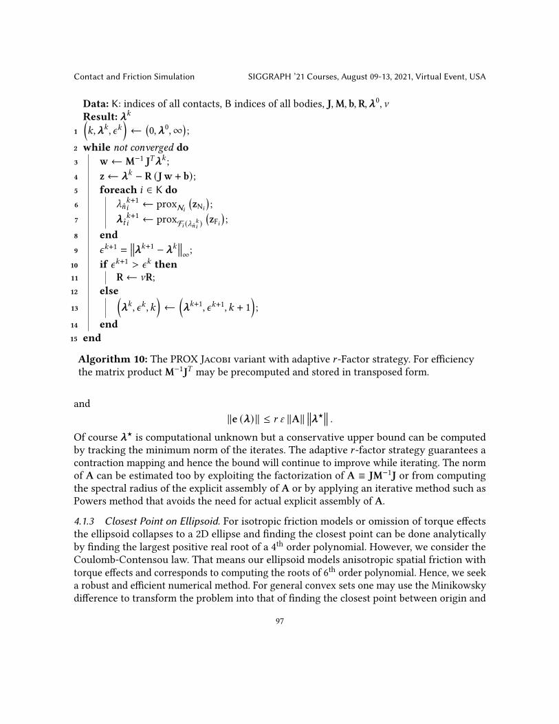
Contact and Friction Simulation SIGGRAPH ’21 Courses, August 09-13, 2021, Virtual Event, USA
Data: K: indices of all contacts, B indices of all bodies, J,M, b,R,𝝀0, aResult: 𝝀𝑘
1
(𝑘,𝝀𝑘 , 𝜖𝑘
)←
(0,𝝀0,∞
);
2 while not converged do3 w← M−1 J𝑇𝝀𝑘 ;4 z← 𝝀𝑘 − R (Jw + b);5 foreach 𝑖 ∈ K do6 _�̂�
𝑘+1𝑖 ← proxN𝑖
(zN𝑖
);
7 𝝀𝑡𝑘+1𝑖 ← proxF𝑖 (_�̂�𝑘𝑖 )
(zF𝑖
);
8 end9 𝜖𝑘+1 =
𝝀𝑘+1 − 𝝀𝑘 ∞;10 if 𝜖𝑘+1 > 𝜖𝑘 then11 R← aR;12 else13
(𝝀𝑘 , 𝜖𝑘 , 𝑘
)←
(𝝀𝑘+1, 𝜖𝑘+1, 𝑘 + 1
);
14 end15 end
Algorithm 10: The PROX Jacobi variant with adaptive 𝑟 -Factor strategy. For efficiencythe matrix productM−1J𝑇 may be precomputed and stored in transposed form.
and∥e (𝝀)∥ ≤ 𝑟 Y ∥A∥
𝝀★ .
Of course 𝝀★ is computational unknown but a conservative upper bound can be computedby tracking the minimum norm of the iterates. The adaptive 𝑟 -factor strategy guarantees acontraction mapping and hence the bound will continue to improve while iterating. The normof A can be estimated too by exploiting the factorization of A ≡ JM−1J or from computingthe spectral radius of the explicit assembly of A or by applying an iterative method such asPowers method that avoids the need for actual explicit assembly of A.
4.1.3 Closest Point on Ellipsoid. For isotropic friction models or omission of torque effectsthe ellipsoid collapses to a 2D ellipse and finding the closest point can be done analyticallyby finding the largest positive real root of a 4th order polynomial. However, we consider theCoulomb-Contensou law. That means our ellipsoid models anisotropic spatial friction withtorque effects and corresponds to computing the roots of 6th order polynomial. Hence, we seeka robust and efficient numerical method. For general convex sets one may use the Minikowskydifference to transform the problem into that of finding the closest point between origin and
97

SIGGRAPH ’21 Courses, August 09-13, 2021, Virtual Event, USA Andrews and Erleben
Data: K: indices of all contacts, B indices of all bodies, J,M, b,R,𝝀0, aResult: 𝝀𝑘
1
(𝑘,𝝀𝑘 , 𝜖𝑘
)←
(0,𝝀0,∞
);
2 while not converged do3 w← M−1 J𝑇𝝀𝑘 ;4 foreach 𝑖 ∈ K do5 I ≡ indices of block N𝑖, F𝑖 ;6 zI ← 𝝀𝑘I − R𝑖 (JIBw + bI);7 _�̂�
𝑘+1𝑖 ← proxN𝑖
(zN𝑖
);
8 𝝀𝑡𝑘+1𝑖 ← proxF𝑖 (_�̂�𝑘+1𝑖 )
(zF𝑖
);
9 w← w +(M−1J𝑇
)B,I
(𝝀𝑘+1I − 𝝀𝑘I
);
10 end11 𝜖𝑘+1 =
𝝀𝑘+1 − 𝝀𝑘 ∞;12 if 𝜖𝑘+1 > 𝜖𝑘 then13 R← aR;14 else15
(_𝑘 , 𝜖𝑘 , 𝑘
)←
(_𝑘+1, 𝜖𝑘+1, 𝑘 + 1
);
16 end17 end
Algorithm 11: The PROX Gauss–Seidel variant with adaptive 𝑟 -Factor strategy. TheproductM−1J𝑇 may be precomputed as for the Jacobi variant.
a convex set. The GJK algorithm is an example of such an algorithm exploiting these ideas.The advantage of a GJK approach is that it is generally applicable to any friction model aslong as the limit surfaces defines a convex set. However, in our case the friction model is anellipsoid and the generality of GJK is uncalled for. Here we present an approach that exploitsthe corresponding 6th order polynomial and apply a root-search method to search for the root.Let 𝑎, 𝑏, 𝑐 > 0 be given. These parameters defines an ellipsoid surface. The ellipsoid surface
consists of all points x ∈ R3 where
𝑓 (x) = x𝑇Kx − 1 = 0 (231)
and K is a positive diagonal matrix given by
K =
1𝑎2 0 00 1
𝑏2 00 0 1
𝑐2
. (232)
98

Contact and Friction Simulation SIGGRAPH ’21 Courses, August 09-13, 2021, Virtual Event, USA
Given a point z ∈ R3 outside the ellipsoid, 𝑓 (z) > 0, then we wish to find the closest point, x★on the ellipsoid surface to z,
x★ = arg min𝑥
12∥x − z∥2 subject to 𝑓 (x) = 0 . (233)
The first order optimality conditions yields
x★ − z − _★∇𝑓 (x★) = 0 . (234)
Using ∇𝑓 (x★) = 2Kx★ and 𝑡 = −2_★ we have,
x★ = (𝑡K + I)−1z . (235)
Further, we must have that x★ lies on the surface of the ellipsoid,
𝑓 (x★) = 𝑓 ((𝑡K + I)−1z) = 0 . (236)
We now define this as a scalar function like this,
𝑔(𝑡) ≡ 𝑓 ((𝑡K + I)−1 z) , (237)
=𝑎2𝑧2
1
(𝑎2 + 𝑡)2+
𝑏2𝑧22
(𝑏2 + 𝑡)2+
𝑐2𝑧23
(𝑐2 + 𝑡)2− 1 . (238)
We observe that our problem of finding the closest point has been reformulated into theproblem of finding a root of 𝑔(𝑡) = 0. From geometry we know that the curve given by 𝑔(𝑡)can pierce an non-degenerate ellipsoid in at most two points. If 𝑓 (z) > 0 then we are seekingthe intersection point with 𝑡 > 0. If 𝑓 (z) ≤ 0 then z is already in the ellipsoid and we simplycan return z as our solution.For 𝑡 > 0 we have 𝑑
𝑑𝑡𝑔(𝑡) < 0. However, 𝑔(𝑡) is very steep for small 𝑡-values and very flat for
larger 𝑡-values. Thus, a binary search numerical method is a good choice for finding the positiveroot of 𝑔(𝑡). Alternatively a Newton-Raphson method can be applied, although Erleben [2017]found a Newton-Raphson method to diverge or find negative roots when the root approachesthe flat parts of the 𝑔-function.An initial bracketing technique is needed for the binary search method. The minimum
𝑡-value for the search interval is given by 𝑡min = 0 the maximum 𝑡-value for the search intervalcan be estimated as,
𝑡guess = max{𝑎, 𝑏, 𝑐}∥z∥ . (239)The maximum 𝑡-value is then given by the minimum non-negative integer, 𝑘 where𝑔(𝑡max) < 0and 𝑡max ≡ 𝛼𝑘𝑡guess, where 𝛼 > 1 is the scalar expansion coefficient of the interval. Erleben[2017] uses 𝛼 = 1.5. In order to make the binary search method more robust in the sense ofhaving better precision the problem can be scaled to be within the unit-cube. That is a scalingfactor is computed as
𝑠 =1
max{1, 𝑎, 𝑏, 𝑐, 𝑧𝑡 , 𝑧𝑏, 𝑧𝜏 }(240)
99

SIGGRAPH ’21 Courses, August 09-13, 2021, Virtual Event, USA Andrews and Erleben
and then re-define the problem as follows.
z← 𝑠 z, and {𝑎, 𝑏, 𝑐} ← {𝑠 𝑎, 𝑠 𝑏, 𝑠 𝑐} . (241)
However, when the scheme has converged one must remember to convert the solution back tothe unscaled problem. The bisection method is summarized in Algorithm 12.
Data: {𝑎, 𝑏, 𝑐}: Ellipsoid shape parameters, z = {𝑧𝑡 , 𝑧𝑏, 𝑧𝜏 }: Query point, 𝜖 > 0: Userspecified accuracy
Result: x The closest point on the ellipsoid1 // Re-scale problem for better numerical precision
2 𝑠 ← 1max(1,𝑎,𝑏,𝑐,|𝑧𝑡 |,|𝑧𝑏 |,|𝑧𝜏 |) ;
3 z← 𝑠 z;4 {𝑎, 𝑏, 𝑐} ← {𝑠 𝑎, 𝑠 𝑏, 𝑠 𝑐};5 // Perform inside ellipsoid test6 if 𝑓 (z) < 𝜖 then7 return z;8 end9 // Perform bracketing for root search
10 𝑡0 ← 0;11 𝑡1 ← max (𝑎, 𝑏, 𝑐) ∥c∥;12 𝛼 ← 1.5 // Expansion coefficient, can be tuned13 while 𝑔(𝑡1) > 0 do14 𝑡1 ← 𝛼 𝑡1;15 end16 // Perform root search and compute closest point17 𝑡∗ ← BisectionRootSearch(𝑔, 𝑡0, 𝑡1, 𝜖);18 𝑡∗ ← 𝑡∗
𝑠2 ;19 x← 𝑡∗ (K + I)−1 z;20 return x;
Algorithm 12: Numerical-Ellipsoid-Solver: Iterative numerical root search method forcomputing the closest point on an ellipsoid.
4.1.4 The 𝑟 -Factor Strategies. If the 𝑟 -value is sufficiently low then the fixed point schemeswill converge as proven by Foerg et al. [2006]; Studer [2008]. Convergence speed is expectedto be worse for small 𝑟 -values than larger 𝑟 -values. Let us study a simple example to buildintuition about how different 𝑟 values affect the fixed point search. For simplicity we will study
100

Contact and Friction Simulation SIGGRAPH ’21 Courses, August 09-13, 2021, Virtual Event, USA
0 0.2 0.4 0.6 0.8 1
0
0.1
0.2
0.3
0.4
0.5
0.6
0.7
0.8
0.9
1Lambda Iterates
r = 0.2
r = 0.4
r = 0.6
r = 0.8
r = 1
0 100 200 300 40010
-16
10-14
10-12
10-10
10-8
10-6
10-4
10-2
100
Fixpoint merit value
r = 0.2
r = 0.4
r = 0.6
r = 0.8
r = 1
Fig. 29. Left figure illustrates the iterates of solving the 2D problem _ = proxS (_ − 𝑟v) where S is a2D disk for different 𝑟 -values. The iterates have been re-scaled by 𝑟/Δ to separate them into distinctcurves for better comparison. On the right the corresponding convergence is displayed. Observe thatthe linear convergence rate constant depends on the 𝑟 -value. Notice that larger 𝑟 -values results in asmaller constant.
a 2D disk S defined by the radius Δ ∈ R+. That isS ≡ {𝝀 ∈ R2 | ∥𝝀∥ ≤ Δ} .
Then we iteratively compute
𝝀𝑘+1 ← proxS(𝝀𝑘 − 𝑟v
).
For a fixed given value of 𝑟 and v ≡[0 1
]𝑇 and 𝝀0 ≡[Δ 0
]𝑇 . The results of solving thissimple 2D example are shown in Figure 29. One can easily observe the benefit of larger 𝑟 -valuesin this simple 2D example. A simple divergence example can be created as well by choosing Sto be the unit disk and solving
𝝀𝑘+1 ← proxS
(𝝀𝑘 − 𝑟
( [2 11 2
]𝝀𝑘 +
[−11
] )).
Using 𝝀0 ≡[0 1
]𝑇 results in the behaviors seen in Figure 30. Here we see the benefit ofincreasing the 𝑟 -value. The iterations in this example are illustrated in Figure 31.
101

SIGGRAPH ’21 Courses, August 09-13, 2021, Virtual Event, USA Andrews and Erleben
0 5 10
iteration
-0.4
-0.2
0
0.2
0.4
0.6
0.8
1
x-v
alue
Iterates
r = 0.4
r = 0.8
r = 1.2
r = 1.6
0 5 10
iteration
-1
-0.8
-0.6
-0.4
-0.2
0
0.2
0.4
0.6
0.8
1
y-v
alue
Iterates
r = 0.4
r = 0.8
r = 1.2
r = 1.6
0 5 10
iteration
0
0.2
0.4
0.6
0.8
1
1.2
1.4
1.6
1.8
2
mer
it v
alue
Convergence
r = 0.4
r = 0.8
r = 1.2
r = 1.6
Fig. 30. Left figure illustrates the iterates of solving the 2D problem _ = proxS (_ − 𝑟 (A_ + b)) whereS is a 2D unit disk for different 𝑟 -values. As one may observe the convergence behavior gets worse forlarger 𝑟 -values in that the iterates starts to oscillate wildly.
Fig. 31. From left to right: the starting iterate, the effect of the first iteration, the second iteration, andfinally a sequence of operations. Observe how the 𝑟 value always "push" the iterate the same distancein the −v direction. Increase 𝑟 -value makes the iterations go faster to the north pole of the disk.
We may apply an adaptive back-tracking approach for adjusting the 𝑟 -values to auto-tunethe 𝑟 -value for better convergence behavior while solving for the fixed point of the proximaloperator. Regardless of chosen strategy, if we detect divergence while iterating, ie. the norm ofthe residual
e𝑘+1 > e𝑘 then we drop updating 𝝀𝑘+1. Instead we roll-back to 𝝀𝑘 and reduce
102

Contact and Friction Simulation SIGGRAPH ’21 Courses, August 09-13, 2021, Virtual Event, USA
all 𝑟 -values by a user specified fraction a . We will next present three different strategies forthe 𝑟 -factors. We call these global, local and blocked strategies.For the global 𝑟 -factor strategy we simply initialize all 𝑟 -values of all constraints to a single
global constant value. Ideally based on theory by Foerg et al. [2006] one should initialize this tothe reciprocal of the sum of the absolute values of the minimum and maximum eigenvalues ofA. However, these are not easily obtained and Erleben [2017] founds that simply hard wiringthe initial 𝑟 -value to say 5 works fine for his examples.For the local 𝑟 -factor strategy one would initially choose the 𝑟 -value of the 𝑖th variable to be
𝑟𝑖 =1A𝑖𝑖
. (242)
Comparing this choice to the algebraic form of the variable updates used in PGS and PSOR weimmediately recognize this as using a PGS-strategy for setting the initial value. If one used𝑟𝑖 =
𝜔A𝑖𝑖
where𝜔 is the successive over-relaxation coefficient then the PSOR variant is achieved,see Section 3.2 for derivation of PGS and PSOR. Hence, one may replace F𝑖 with a box-modeland keeping local 𝑟 -values as fixed constants and the PROX scheme will deteriorate into thewell known PGS/PSOR variants used in may physics engines.For the blocked strategy the idea is to replace the scalar 𝑟 -values with small blocked matrices
build from the diagonal blocks of the A-matrix. Let us consider the 𝑘 th block corresponding tothe 𝑘 th contact, then the 𝑟 -factor strategy uses the block R𝑘 ∈ R4×4,
R𝑘 =[ 1A𝑖𝑖
00 A−1
𝑡 :𝜏,𝑡 :𝜏
], (243)
where 𝑛 = 4𝑘 , 𝑡 = 𝑛+1, 𝑏 = 𝑛+2, 𝜏 = 𝑛+3. The blocked strategy has been reported by Merlhiot[2007] to work quite well.For the global and blocked strategies one may use a = 0.5 and for the local strategy a = 0.9.
These values are not critical but was tuned experimentally and reported by Erleben [2017]. Note𝑟 -factors are not the same as numerical damping or regularization as known from LCP methodsshown in Cottle et al. [1992]. For those the coefficient matrix is changed like A ← I𝜌 + Afor some damping parameter 𝜌 > 0. This changes the model and adds compliance to thecontact. The 𝑟 -factors does not change the model, the solutions hold for all positive 𝑟 -values.The specific 𝑟 -value only affect the convergence constants. Erleben [2017] reports that local𝑟 -value strategy combined with Gauss-Seidel type variant of PROX gives more predictableperformance in most cases, and that the global strategy for Jacobi scheme has interestingcapabilities for dealing with large structured stacks like masonry structures.
4.1.5 Time-Stepping Methods. The PROX schemes can be used with different time-steppingmethods. In this presentation we favor the mid-point scheme of Moreau [1999]. It consists ofusing an explicit half-step position update
q𝑡+12 = q𝑡 + ℎ
2Hu𝑡 . (244)
103
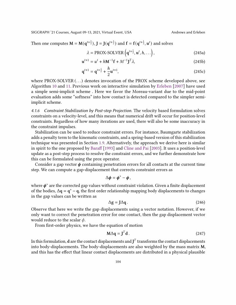
SIGGRAPH ’21 Courses, August 09-13, 2021, Virtual Event, USA Andrews and Erleben
Then one computesM = M(q𝑡+ 12 ), J = J(q𝑡+ 1
2 ) and f = f (q𝑡+ 12 , u𝑡 ) and solves
_ = PROX-SOLVER(q𝑡+
12 , u𝑡 , ℎ, . . .
), (245a)
u𝑡+1 = 𝑢𝑡 + ℎM−1f +𝑀−1J𝑇_, (245b)
q𝑡+1 = q𝑡+12 + ℎ
2u𝑡+1, (245c)
where PROX-SOLVER (. . .) denotes invocation of the PROX scheme developed above, seeAlgorithm 10 and 11. Previous work on interactive simulation by Erleben [2007] have useda simple semi-implicit scheme . Here we favor the Moreau-variant due to the mid-pointevaluation adds some “softness” into how contact is detected compared to the simpler semi-implicit scheme.
4.1.6 Constraint Stabilization by Post-step Projection. The velocity based formulation solvesconstraints on a velocity-level, and this means that numerical drift will occur for position-levelconstraints. Regardless of how many iterations are used, there will also be some inaccuracy inthe constraint impulses.Stabilization can be used to reduce constraint errors. For instance, Baumgarte stabilization
adds a penalty term to the kinematic constraints, and a spring-based version of this stabilizationtechnique was presented in Section 1.9. Alternatively, the approach we derive here is similarin spirit to the one proposed by Baraff [1993] and Cline and Pai [2003]. It uses a position-levelupdate as a post-step process to resolve the constraint errors, and we further demonstrate howthis can be formulated using the prox operator.Consider a gap vector 𝝓 containing penetration errors for all contacts at the current time
step. We can compute a gap-displacement that corrects constraint errors as
Δ𝝓 = 𝝓∗ − 𝝓 ,where 𝝓∗ are the corrected gap values without constraint violation. Given a finite displacementof the bodies, Δq = q∗ − q, the first order relationship mapping body displacements to changesin the gap values can be written as
Δg = JΔq . (246)Observe that here we write the gap displacements using a vector notation. However, if weonly want to correct the penetration error for one contact, then the gap displacement vectorwould reduce to the scalar 𝜙 .From first-order physics, we have the equation of motion
MΔq = J𝑇d . (247)
In this formulation, d are the contact displacements and J𝑇 transforms the contact displacementsinto body-displacements. The body-displacements are also weighted by the mass matrixM,and this has the effect that linear contact displacements are distributed in a physical plausible
104

Contact and Friction Simulation SIGGRAPH ’21 Courses, August 09-13, 2021, Virtual Event, USA
way as linear and rotational displacements of the bodies. From the above equation of motion,we can write the body-displacements as
Δq = M−1J𝑇d . (248)
Next, we substitute into our kinematic gap-equation to derive1
Δ𝝓 = JM−1J𝑇d . (249)
We seek a body displacement such that the gap-function becomes non-negative,
𝝓∗ = (Δ𝝓 + 𝝓) ≥ 0 . (250)
Recall that contact displacements can only “push” bodies apart, which means that d ≥ 0, andfurthermore we cannot have a contact displacement at a separated contact. Thus, we wish tofind a body displacement such that
(Δ𝝓 + 𝝓) ≥ 0, d ≥ 0 and d𝑇 (Δ𝝓 + 𝝓) = 0 . (251)
Combining these yields(JM−1J𝑇d + 𝝓
)≥ 0, d ≥ 0 and d𝑇
(JM−1J𝑇d + 𝝓
)= 0 , (252)
which is a linear complementarity problem. This can be re-cast as a proximal operator model
d = proxN(d − 𝑟
(JM−1J𝑇d + 𝝓
))(253)
for all 𝑟 > 0 whereN = N1× · · · ×N𝑛 . Having solved for d a position update can be performed.
q∗ = q + H(q)M−1J𝑇d . (254)
Recall thatH(q) is the kinematic mapping between velocities and positions. The above equationcan be seen as computing an instantaneous change of the body positions disregarding velocities,external forces or velocity dependent forces. The scheme is of course based on a linearizationof the true gap-function. Therefore, it may not be able to resolve the errors with a single stepand quite often several steps must be taken.
4.2 Anisotropic FrictionThe isotropic Coulomb friction model is used by many rigid body simulations in the fieldof computer graphics [Bender et al. 2014], and indeed the focus of these has been on thedifficult problem of formulating and solving isotropic Coulomb frictional contact and itsapproximations. However, there has been comparatively less attention in computer graphicson more expressive anisotropic models of frictional contact. Nevertheless, various frameworkshave been developed in recent years for simulating anisotropic friction in computer graphics.For instance, friction tensors [Pabst et al. 2009] and the Matchstick model [Erleben et al. 2020].The methodology presented in this section is inspired by the latter.
105

SIGGRAPH ’21 Courses, August 09-13, 2021, Virtual Event, USA Andrews and Erleben
Fig. 32. The Matchstick model allows for control of frictional behavior in situations such as tire groundcontact, a hopper, and soft robotic gripping, where each example shown here also uses differentsimulators with different contact solvers (Vortex, PROX, and Flex).
As shown in Section 1, many physics simulators use friction models expressed as conesor as generic sets of feasible friction forces. Combining feasible set descriptions with extraconstraints, such as the principle of maximum dissipation, allows us to compute the frictionforces at a given instant in time. The benefit of such friction descriptions is that they permit aneasy implementation within a simulator. One can define a projection operator, and iterativelyproject the friction force onto the closest feasible friction force. This property is the governingprinciple about which many friction models can be defined.The Matchstick model produces a cone based on surface structural directions from each
body at the point of contact. Figure 32 shows simulation examples using this model.
4.2.1 Friction Cone Modeling. We begin by examining how to generate an anisotropic frictioncone based on the kinematic state of two bodies, A and B. The main idea here is to create aconvex pointed cone based on the relative orientation between the two surfaces.An important difference of anisotropic friction compared to isotropic friction is that the
local material frame of each surface is considered. For instance, with regards to the Matchstickmodel, the structural directions on each surface are defined with respect to some materialframe. The directions can be interpreted as fiber directions or as micro-scale geometry features,such as grooves. While other materials, e.g., cloth with warp and weft directions, can be seenas having multiple material directions. For the sake of brevity, we limit our presentation to thecase of a single material direction.For any given contact frame (see Figure 4), the material direction of each surface can be
written as unit vectors sA and sB, in the space of the tangent plane. These directions dependon the point of contact on each surface, and in a typical implementation they can be stored ina texture or generated procedurally. Given a simple parameterized cone generator, GA↔B, thatcomputes a friction cone that describes the set of allowable friction forces based on the set oflocal parameters, we denote the generated cone by the symbol FA↔B. Relaxing the notationand not explicitly writing the object pairs, the generator can be defined as
F ≡ G (_�̂�, v𝑡 , sA(p), sB(p)) . (255)
106

Contact and Friction Simulation SIGGRAPH ’21 Courses, August 09-13, 2021, Virtual Event, USA
Fig. 33. The angle betweenmatchsticks determines the friction cone. TheMatchstickmodel interpolatesbetween isotropic C𝐼 and anisotropic C𝐴 extremes (see Equations 258, 261, and 264).
The normal force magnitude is given by _�̂�. The above parameterization could be extendedwith even more parameters to account for other dependencies. However, F here simply refersto any parametric friction cone model to enhance readability.
4.2.2 The Matchstick Model. Next, we derive the Matchstick model for the framework ofanisotropic friction outlined in the previous section. The model is a phenomenological one,and it is based on several observations about how surfaces with structural features interact asthey slide against each other (see Figure 33). Briefly, the frictional behavior appears isotropicfor a pair of matchsticks when moving in different direction, but keeping structure directionsorthogonal. Whereas the behavior is anisotropic for a pair of matchsticks when sliding indifferent directions while keeping structure directions parallel. The model thus interpolatesbetween isotropic and anisotropic Coulomb behaviors using the minimum angle between thestructural directions.With the simplifying assumption that the sign of the structure vector s can be ignored (i.e., if
the friction only depends on the orientation and not the direction), then the Matchstick modelinterpolation parameter is based on the angle \ , and it is defined as
𝑑 ≡ 1 − 2𝜋
cos−1 |sA · sB |︸ ︷︷ ︸≡\
. (256)
Let the friction force in the world frame be given by f and let the coefficient of friction for aplanar isotropic Coulomb friction cone be `, equal to the tangent 𝑡 and binormal 𝑏 directioncoefficients for the isotropic cone, i.e.,
`𝐼𝑡= `𝐼
𝑏= ` , (257)
107

SIGGRAPH ’21 Courses, August 09-13, 2021, Virtual Event, USA Andrews and Erleben
then the isotropic cone is defined by the relationship
f𝑇R𝑇[
1`
2 00 1
`
2
]︸ ︷︷ ︸≡C𝐼
Rf ≤ _�̂�2 . (258)
Here, R can be any rotation matrix for an isotropic cone, but for consistency we define R asthe 2D rotation of (sA + sB) onto the 𝑡 axis, assuming that sA · sB is positive (given that onlythe orientation is needed, we can swap the sign of one of the vectors to ensure positive dotproduct). This implies that the tangent plane vectors are defined as
𝑡 ≡ sA + sB∥sA + sB∥
, (259)
𝑏 ≡ �̂� × 𝑡 . (260)
By construction, 𝑡 and𝑏 are themajor andminor axis of the anisotropic ellipse cone, respectively.And while the planar rotation matrix R is useful for explaining the model, the column vectors𝑡 and 𝑏 are needed when assembling the Jacobian matrix.For anisotropic Coulomb friction, the coefficients of friction are `𝐴
𝑡≤ `𝐴
𝑏, where the 𝐴
superscript denotes anisotropy. Similar to the isotropic case, the anisotropic cone is defined bythe quadratic inequality
f𝑇R𝑇
1`𝐴𝑡
2 0
0 1`𝐴𝑏
2
︸ ︷︷ ︸≡C𝐴
Rf ≤ _�̂�2 . (261)
In the case of the Matchstick model, the friction cone generator G computes the coefficientsby a spherical linear interpolation between the isotropic and anisotropic cones, such that
`𝑡 ≡ 𝑑 `𝐴𝑡 + (1 − 𝑑) ` , (262)
`𝑏≡ 𝑑 `𝐴
𝑏+ (1 − 𝑑) ` . (263)
Thus, the actual Coulomb cone based on the kinematic configuration is given by:
f𝑇R𝑇[
1`𝑡
2 00 1
`𝑏
2
]︸ ︷︷ ︸≡C𝑀
Rf ≤ _2𝑛 . (264)
The Matchstick friction model generator is outlined in Algorithm 13. A nice aspect about themodel is that it has a small memory footprint and fast computational complexity for generatingthe cone and using it at run time. In the next section we will outline how the Matchstick model
108

Contact and Friction Simulation SIGGRAPH ’21 Courses, August 09-13, 2021, Virtual Event, USA
Data: Structure directions sA, sB, contact normal �̂�, isotropic friction `, extreme frictioncoefficients `𝐴
𝑡, `𝐴𝑏.
Result: Contact plane vectors 𝑡 , 𝑏, and coefficients of friction `𝑡 , `𝑏 .1 if sA · sB < 0 then2 sB ← −sB;3 end4 \ ← cos−1 (sA · sB);5 𝑑 ← 1 − 2\
𝜋;
6 `𝑡 ← 𝑑 `𝐴𝑡+ (1 − 𝑑) `;
7 `𝑏← 𝑑 `𝐴
𝑏+ (1 − 𝑑) `;
8 𝑡 ← sA+sB∥sA+sB∥ ;
9 𝑏 ← �̂� × 𝑡 ;
Algorithm 13: MatchStickFrictionGenerator The generator gives both the worldorientation of the friction cone as well as the coefficients of friction, which is an advantagewhen working with an analytic cone that is fully described by these parameters.
can be incorporated into different modeling approaches and solvers, before we conclude ourpresentation with some implementation notes. Thereby we demonstrate the Matchstick modelto be a general model suitable for any type of simulator.
4.2.3 Fixed-point Solvers. We will now present how the Matchstick model can be used in asolver. Iterative methods for contact force computations are the natural choice for arbitraryfriction cones. We will first consider the class of methods based on proximal operators asdescribed in Section 4.1. In methods based on proximal operators, the next feasible frictionimpulse iterate 𝝀𝑡𝑘+1 is given by projecting the current guess 𝝀𝑡𝑘 onto the friction cone, suchthat
𝝀𝑡𝑘+1 ← proxF
(𝝀𝑡𝑘 − 𝑟𝑡 v𝑡𝑘
), (265)
and tangential forces 𝝀𝑡 =[_𝑡 _
𝑏
]𝑇 are projected into the anisotropic cone
F ≡{𝝀𝑡
�����(_2𝑡
`2𝑡
+_2𝑏
`2𝑏
)≤ _�̂�2
}. (266)
Here, 𝑘 is the iteration index and 𝑟𝑡 is a scalar relaxation parameter known as the 𝑟 -factor. Thealgorithm then proceeds using a sweeping process. First, Equation 255 is used to instantiatethe current friction cone, F , and then that cone is used in the proximal point update givenby Equation 265. Algorithm 14 illustrates how a PROX-based block Gauss-Seidel variant is
109

SIGGRAPH ’21 Courses, August 09-13, 2021, Virtual Event, USA Andrews and Erleben
Data: Indices of all contacts K, indices of all bodies B, and J, M, b, 𝑟 , 𝝀0, a .Result: 𝝀𝑘
1
(𝑘,𝝀𝑘 , 𝜖𝑘
)←
(0,𝝀0,∞
);
2 while not converged do3 w← M−1 J𝑇𝝀𝑘 ;4 foreach 𝑖 ∈ K do5 I ≡ indices of block N𝑖, F𝑖 ;6 zI ← 𝝀𝑘I − 𝑟 (JIBw + bI);7 _𝑘+1𝑛 ← proxN𝑖
(z𝑛);8 F ← G(_�̂�𝑘+1𝑖 , . . .);9 𝝀𝑡
𝑘+1𝑖 ← proxF
(zF𝑖
);
10 w← w +(M−1J𝑇
)BI
(𝝀𝑘+1I − 𝝀𝑘I
);
11 end12 𝜖𝑘+1 =
𝝀𝑘+1 − 𝝀𝑘 ∞;13 if 𝜖𝑘+1 > 𝜖𝑘 then14 𝑟 ← a𝑟 ;15 else16
(𝝀𝑘 , 𝜖𝑘 , 𝑘
)←
(𝝀𝑘+1, 𝜖𝑘+1, 𝑘 + 1
);
17 end18 end
Algorithm 14: ProxGaussSeidel The PROX Gauss-Seidel variant with an adaptive global𝑟 -Factor strategy and parametric friction cones. The product M−1J𝑇 may be precomputed.
modified to accommodate such friction models. Observe that the only change is the addition ofline 8 in the algorithm, before the friction proximal step, which instantiates the friction model.
4.2.4 LCP-based Solvers. For LCP based approaches, one may discretize a parameterized coneby shooting rays from the origin of the limit surface in various directions and use the limitsurface points to build a polygonal approximation to the generated cone, such as the oneshown in Figure 6. Each facet of the polyhedral cone will match one complementary constraintin the LCP model. While it is trivial to generate the polygonal facets, the main drawback isthat one may need many facets to obtain a good approximation. The memory footprint of thepolyhedral LCP has quadratic scaling with the number of constraints and the solver time willsuffer accordingly. Hence, nonlinear complementary formulations can be more attractive forparametric cones.
110

Contact and Friction Simulation SIGGRAPH ’21 Courses, August 09-13, 2021, Virtual Event, USA
4.2.5 NCP-based Solvers. Let us consider how to use a parameterized cone F in a Newton typeframework by using non-smooth functions, such as the Fischer-Burmeister function [Macklinet al. 2019]. Without loss of generality, assume we have any type of complementary function,𝜓 (𝑎, 𝑏) : R × R ↦→ R such that
0 ≤ 𝑎 ⊥ 𝑏 ≥ 0 ⇔ 𝜓 (𝑎, 𝑏) = 0 . (267)
Using an implicit limit surface of the cone we let [ be the corresponding implicit function ofF ,
[ ≡ f𝑇R𝑇C𝑀Rf − _�̂�2. (268)
Then by the principle of maximal dissipation we can write
∇[ (f) = −𝛽 v𝑡 , (269)
where 𝛽 ≥ 0 is an auxiliary scalar variable. We can now restate the model with the help of thecomplementary function,
𝜓 (𝛽,−[ (f)) = 0 , (270)
𝜓 (v𝑡𝑇v𝑡 ,w𝑇w) = 0 , (271)
where we now introducew = ∇[ (f) +𝛽 v𝑡 . The above model gives us a root search problem andcan be solved with a Newton type of method. For this purpose we must obtain the generalizedJacobian of these equations. The differential becomes
𝑑𝜓 (𝛽,−[ (f)) = 𝜕𝑎𝜓 𝑑𝛽 − 𝜕𝑏𝜓 ∇[𝑇𝑑f , (272)
𝑑𝜓 (v𝑡𝑇v𝑡 ,w𝑇w) = 2𝜕𝑎𝜓 v𝑡𝑇𝑑v𝑡 + 2𝜕𝑏𝜓 w𝑇𝑑w , (273)
where𝑑w = v𝑡 𝑑𝛽 + ∇2[ 𝑑f + 𝛽 𝑑v𝑡 . (274)
Here we use ∇2 to denotes the Hessian of [. Assembling all parts we can write[𝑑𝜓 (𝛽,−[ (f))𝑑𝜓 (v𝑡𝑇v𝑡 ,w𝑇w)
]= J𝜓
𝑑𝛽
𝑑f𝑑v𝑡
(275)
where J𝜓 is the Jacobian one will need for implementing a Newton method, and is computed as
J𝜓 ≡[
𝜕𝑎𝜓 −𝜕𝑏𝜓 ∇[𝑇 02(𝜕𝑏𝜓w𝑇v𝑡
)2(𝜕𝑏𝜓w𝑇∇2[
)2(𝜕𝑎𝜓v𝑡𝑇 +𝜕𝑏𝜓w𝑇𝛽
) ] .Figure 34 shows examples of Flex which uses a fully implicit solver based on a Newton
method using a Fischer-Burmeister formulation.
111

SIGGRAPH ’21 Courses, August 09-13, 2021, Virtual Event, USA Andrews and Erleben
Fig. 34. A structure field on a ravine slope can be used to steer a log slide towards (top) or around(bottom) a cube-shaped building.
4.2.6 Implementation Notes. Notice that a friction cone generator G, such as the one inAlgorithm 13, returns not only a friction cone F , but also the cone orientation C ≡
[�̂� 𝑡 𝑏
].
Here, C is needed for the assembly of the contact Jacobian, as is evident from Equation 22.Hence, one may wish to invoke the generator when assembling the contact Jacobian or splitthe generator implementation into two sub-routines– one for computing the cone and one fordetermining the contact frame. The choice is intimately related to how the time-discretizationof the friction cone is implemented. Imagine that the cone generator parametrically dependson the sliding velocity v𝑡 and that a fully implicit integration scheme is wanted. In this case,the generator truly needs to be invoked each time before projecting 𝝀𝑡 to the cone. However,in most cases the positions and orientations are not updated inside the solver algorithm asshown in Algorithm 14, and both the cone orientation and limit surface can be computedoutside the solver for improved computational efficiency. However, for the Newton type solveroutlined above, one must update cone orientations continuously as positions and velocitiesare solved in a fully coupled way, which gives a fully implicit time-integration method.We note that an additional torque can be included in the friction model, which introduces an
angular moment about the contact normal based on an additional friction coefficient, `𝜏 . Thevalue of this coefficient is computed similar to `𝑡 and `𝑏 , and this type of torsional frictionis also known as a Coulomb–Contensou friction model. Inclusion of this torque is optionalfrom a modeling perspective, but does result in a higher-dimensional limit surface, and thusrequires a third diagonal term in C as 1
`𝜏
2, thus promoting R to a 3D rotation matrix. Theproximal operator for this surface can then be solved numerically, as outlined in Section 4.1.3,whereas omitting this additional term gives a planar surface and the projection can be solvedanalytically.
112
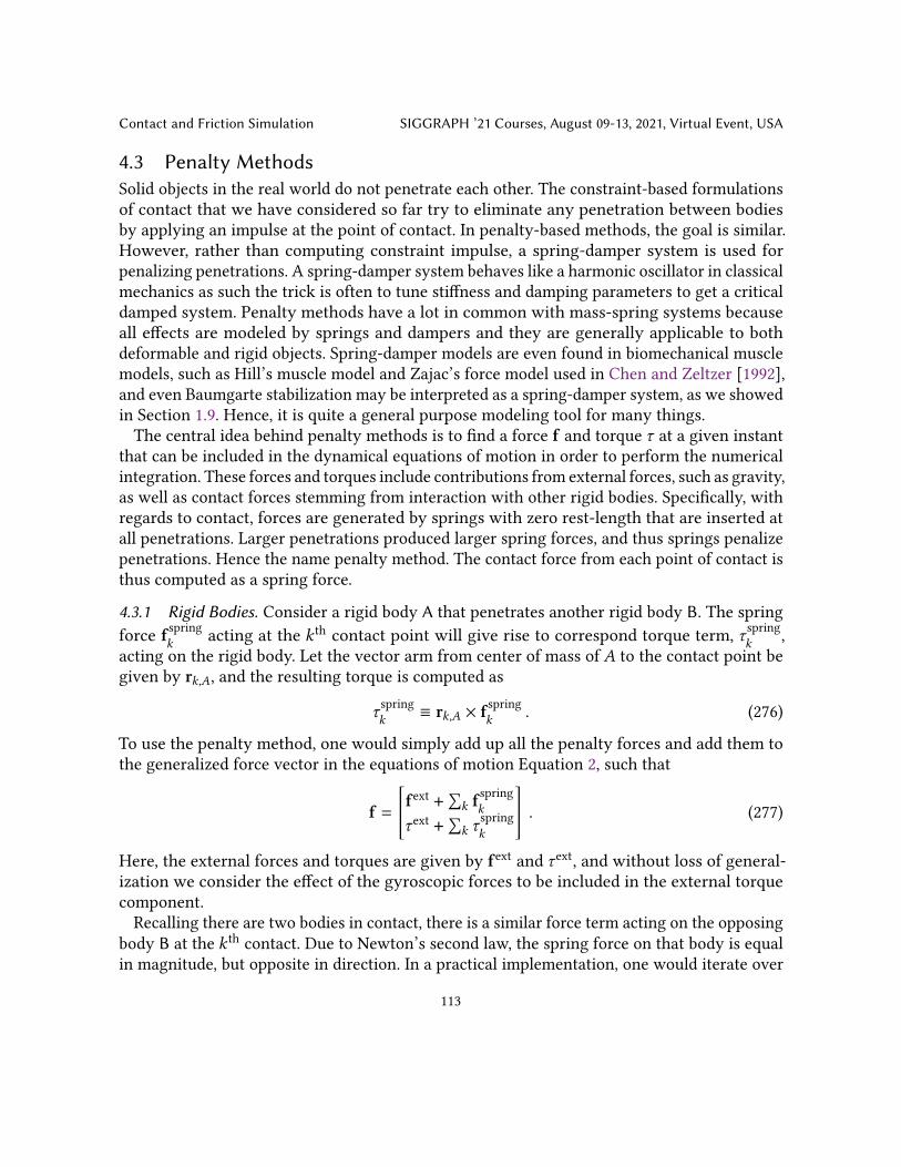
Contact and Friction Simulation SIGGRAPH ’21 Courses, August 09-13, 2021, Virtual Event, USA
4.3 Penalty MethodsSolid objects in the real world do not penetrate each other. The constraint-based formulationsof contact that we have considered so far try to eliminate any penetration between bodiesby applying an impulse at the point of contact. In penalty-based methods, the goal is similar.However, rather than computing constraint impulse, a spring-damper system is used forpenalizing penetrations. A spring-damper system behaves like a harmonic oscillator in classicalmechanics as such the trick is often to tune stiffness and damping parameters to get a criticaldamped system. Penalty methods have a lot in common with mass-spring systems becauseall effects are modeled by springs and dampers and they are generally applicable to bothdeformable and rigid objects. Spring-damper models are even found in biomechanical musclemodels, such as Hill’s muscle model and Zajac’s force model used in Chen and Zeltzer [1992],and even Baumgarte stabilization may be interpreted as a spring-damper system, as we showedin Section 1.9. Hence, it is quite a general purpose modeling tool for many things.The central idea behind penalty methods is to find a force f and torque 𝜏 at a given instant
that can be included in the dynamical equations of motion in order to perform the numericalintegration. These forces and torques include contributions from external forces, such as gravity,as well as contact forces stemming from interaction with other rigid bodies. Specifically, withregards to contact, forces are generated by springs with zero rest-length that are inserted atall penetrations. Larger penetrations produced larger spring forces, and thus springs penalizepenetrations. Hence the name penalty method. The contact force from each point of contact isthus computed as a spring force.
4.3.1 Rigid Bodies. Consider a rigid body A that penetrates another rigid body B. The springforce f spring
𝑘acting at the 𝑘 th contact point will give rise to correspond torque term, 𝜏 spring
𝑘,
acting on the rigid body. Let the vector arm from center of mass of 𝐴 to the contact point begiven by r𝑘,𝐴, and the resulting torque is computed as
𝜏spring𝑘
≡ r𝑘,𝐴 × f spring𝑘. (276)
To use the penalty method, one would simply add up all the penalty forces and add them tothe generalized force vector in the equations of motion Equation 2, such that
f =
[fext +∑
𝑘 fspring𝑘
𝜏ext +∑𝑘 𝜏
spring𝑘
]. (277)
Here, the external forces and torques are given by fext and 𝜏ext, and without loss of general-ization we consider the effect of the gyroscopic forces to be included in the external torquecomponent.Recalling there are two bodies in contact, there is a similar force term acting on the opposing
body B at the 𝑘 th contact. Due to Newton’s second law, the spring force on that body is equalin magnitude, but opposite in direction. In a practical implementation, one would iterate over
113

SIGGRAPH ’21 Courses, August 09-13, 2021, Virtual Event, USA Andrews and Erleben
contact points and compute the penalty force only once per contact and then distribute thespring force to the two bodies that are in contact. In its most pure form the simulation loop ofthe penalty method can now be summarized as
• Detect contact points (run collision detection).• Compute and accumulate spring forces.• Integrate equations of motion forward in time.
This is the pure form of the penalty method. In practice, it is combined with several othertechniques, some of which we will elaborate on below.First we will turn our attention toward the actual computation of the penalty forces in a
general simulator. Let the 𝑘 th contact point between the two bodies 𝐴 and 𝐵 with center ofmass at x𝐴 and x𝐵 respectively be at position p𝑘 given in 3D world coordinates. The 𝑘 th contactpoint has the contact normal, n𝑘 , also in 3D world space, pointing from body 𝐴 toward body 𝐵,and a measure of penetration depth, 𝜙𝑘 . Then the penalty force acting on body 𝐵 is given by
f spring𝐵
= (−𝑘𝜙𝑘 − 𝑏v𝑘 · �̂�𝑘) �̂�𝑘 , (278)
where v𝑘 denotes the relative contact velocity at the 𝑘 th contact point. Observe, that thepenalty force here only works in the normal direction of the contact. Hence, we are currentlyignoring friction. The coefficients 𝑘 and 𝑏 are known as the stiffness and damping coefficients,sometimes the stiffness coefficient is referred to as the spring constant as well. The term v𝑘 · �̂�𝑘is essentially only measuring the relative velocity in the normal direction, let us define thisas 𝑣�̂�,𝑘 = v𝑘 · �̂�𝑘 . For 𝑣�̂�,𝑘 < 0 objects are approaching each other, 𝑣�̂�,𝑘 = 0 there is no relativemovement, and if 𝑣�̂�,𝑘 > 0 objects are moving away from each other. Notice how carefullythe viscosity is modeled only to work in the direction of the contact normal to ensure thatdamping should only work in the constraint direction. We may compute 𝑣�̂�,𝑘 like this
𝑣�̂�,𝑘 = �̂�𝑘 ·( (v𝐴 + 𝜔𝐴 × r𝑘,𝐴
)−
(v𝐵 + 𝜔 𝑗 × r𝑘,𝐵
) ), (279)
= �̂�𝑇𝑘
[I3×3 −r×𝑘,𝐴 −I3×3 r×
𝑘,𝐵
]︸ ︷︷ ︸J𝑘
v𝐴𝜔𝐴v𝐵𝜔𝐵
︸︷︷︸u
= J𝑘u , (280)
where r𝑘,𝐴 = p𝑘 − x𝐴 and r𝑘,𝐵 = p𝑘 − x𝐵 . We have seen this before in Equation 17, and if wehad a soft body instead of a rigid body then the normal relative velocity can be computed aswe did in Equation 20. If we write up the magnitude of the spring force as
_�̂�,𝑘 ≡ −𝑘𝜙𝑘 − 𝑏 ¤𝜙𝑘 . (281)
114

Contact and Friction Simulation SIGGRAPH ’21 Courses, August 09-13, 2021, Virtual Event, USA
Here, we use the substitution that ¤𝜙𝑘 = 𝑣�̂�,𝑘 and with this notation in place we can write thespring forces and torques on body A and B as follows:
f spring𝐴
𝜏spring𝐴
f spring𝐵
𝜏spring𝐵
=
−�̂�𝑘_�̂�,𝑘
−r𝑘,𝐴 × �̂�𝑘_�̂�,𝑘�̂�𝑘_�̂�,𝑘
r𝑘,𝐴 × �̂�𝑘_�̂�,𝑘
= −J𝑇𝑘_�̂�,𝑘 . (282)
It is interesting to generalize Equation 279 and Equation 282 to a system with multiple bodiesand multiple contacts. Hence, let us do this. We obtain,
¤𝝓 = Ju , (283a)𝝀 = −K𝝓 − B ¤𝝓 , (283b)
M ¤u = f + J𝑇λ , (283c)here K is a diagonal matrix with stiffness coefficients, B a diagonal matrix with dampingcoefficients, and λ is a vector of spring force magnitudes. The vector u is the generalizedvelocities andM is the mass matrix, and J is the system Jacobian matrix. If we have 𝐾 contactsand 𝑁 rigid bodies then 𝝓, ¤𝝓,λ ∈ R𝐾 , and f, u ∈ R6𝑁 , J ∈ R𝐾×6𝑁 , M ∈ R6𝑁×6𝑁 , and K,B ∈R𝐾×𝐾 .
4.3.2 Soft Bodies. In case of soft bodies, dimension 6𝑁 is replaced with 3𝑉 , where 𝑉 isthe total number of vertices in the system. However, note that for soft bodies, there is notorque component generated by the spring forces (meaning the last row of Equation 277 isdropped). Also note that for soft bodies, the contact point may not coincide with a node of thecomputational mesh. In this case, the penalty force is often distributed to the enclosing nodesof the contact point using some weighting scheme. The most common choice for computergraphics is to use linear weights based on the barycentric coordinates of the nodes. With theseconsiderations, it is trivial to perform a time-discretization to Equation 283 in order to solvethis system of ordinary differential equations. Xu et al. [2014] showed how to take the ideaswe presented here into an implicit time-stepping scheme.
4.3.3 Implementation Notes. It is quite interesting to compare the penalty method algebraicform given in Equation 283 with that of a constraint based method. We observe that theJ-matrices appear in similar places, but 𝝀 is now given by a closed-form solution. The springforce, or rather impulses, are simply computed by evaluating Equation 283 at the instantcorresponding to the chosen time-stepping scheme. Hence, the per-time-step complexity of thepenalty method is very fast compared to solving an LCP problem per time-step. Furthermore,in most implementations of the penalty method, the above matrices are not assembled, whichfurther reduces the computational and storage complexity. Yet the algebraic form here providesa straightforward connection to the constraint based approaches that we have already coveredin full detail.
115

SIGGRAPH ’21 Courses, August 09-13, 2021, Virtual Event, USA Andrews and Erleben
There are, however, several difficulties associated with the classical penalty method. Theseare listed below without going into details about possible solutions:• It is not trivial to compute satisfactory contact normals or penetration depths as they lackglobal knowledge about the entire state. The problem of determining meaningful contactnormals and penetration depths is mostly caused by the use of local computations. If aglobal computation [Kim et al. 2002] is used instead, these problems can be resolved.• Some contact points like the face-face case appearing in a box stack is difficult to handleby applying a penalty force at the contact point of deepest penetration [Hasegawa et al.2003]. To alleviate this problem, researchers have tried to sample the entire contact regionwith contact points. There also exist methods, that integrate over the intersection areaand/or volume.• During motion, there can be a discontinuous changes of the contact normals.• It is not trivial to pick the stiffness and damping parameters. Stiffness parameter need tobe large enough to remove any penetration. Unfortunately, this value limits the time-stepsize severely for explicit time-stepping methods.• The springy nature of the contact forces can create secondary oscillation effects that leadsto a more “spongy” contact behavior than the hard contact response that is expected fromrigid bodies.
4.3.4 Penalty Based Friction. Until now, we have only been concerned with generating non-interpenetration forces using penalty methods. How should one go about modeling friction ina penalty-based simulator? It seems reasonable to use a spring-damper system for the frictionforce as well. This is often done by tracking the contact points. At first point of contact, ananchor point a, is saved. This is an unmovable point in the world coordinate system. Thefriction force is determined by the spring force stemming from the zero-length spring withstiffness coefficient 𝑘 between the anchor point and the current position p of the contact pointthat caused the creation of the anchor point:
f springfriction = 𝑘 (a − p) . (284)
The value of the friction stiffness coefficient it typically different from the value of the normalstiffness coefficient. During subsequent time steps, the simulation is monitored to ensure thefollowing condition holds: f springfriction
≤ ` f spring , (285)
here, ` is the Coulomb coefficient of friction and f spring is the normal penalty force. If thecondition is fulfilled, we have the case of static friction and nothing needs to be done. If, onthe other hand, the condition is broken, then we have the case of dynamic friction (sliding)and the anchor point is moved towards the current contact position p such that the conditionin Equation 285 is true.
116

Contact and Friction Simulation SIGGRAPH ’21 Courses, August 09-13, 2021, Virtual Event, USA
The frictional spring force model can be physically justified as a crude model of the externalshear stresses acting between two bodies. As such, the friction model adds an elementof compliance to the rigid bodies. Another approach to model friction is as a dampingforce [McKenna and Zeltzer 1990], like this,
f springfriction = −` f spring v𝑡
∥v𝑡 ∥, (286)
where v𝑡 is the tangential relative sliding velocity. This approach only models dynamic friction,thus static friction is ignored.
4.3.5 Other Penalty Methods. We will now briefly survey a few of the usual tricks and ideasthat have been used in the context of penalty methods over the years in the field of computergraphics. Our coverage is not complete but most central ideas are represented. Moore andWilhelms [1988] were among the first to model contact forces by springs in computer animation.They used a simple linear spring, but added a twist of letting the spring constant depend onwhether the motion is receding or approaching. The relationship is as follows
𝑘recede = Y𝑘approach , (287)where Y describes the elasticity of the collision, Y = 0 corresponds to totally inelastic collisions,and Y = 1 to perfectly elastic collisions. Furthermore, Moore and Wilhelms extended thepenalty method with an algebraic collision resolving method, similar to Newton’s collisionlaw. The main idea is to handle colliding contacts before applying springs. This is becausecolliding contacts requires very stiff springs, which are numerically intractable.Terzopoulos et al. [1987] used another kind of penalty force. The main idea behind their
derivation comes from conservative forces, which are known to be the negative gradient of aenergy potential, that is the negative gradient of a scalar function. A scalar energy function isthen designed that penalizes penetration, such that
𝑐 exp(−𝜙Y
), (288)
where 𝑐 and Y are constants used to determine the specific shape of the energy potential. Thepenalty force is then computed as
f spring = −(∇𝜙Y
exp(−𝜙Y
)· �̂�
)�̂� . (289)
Such penalty forces are called exponential springs. Exponential springs are stiffer for largedisplacement than linear springs, which can quickly lead to stability problems for explicitintegration schemes. However, for small displacements exponential springs are less stiff thanlinear springs [McKenna and Zeltzer 1990].McKenna and Zeltzer [1990] introduce a twist on penalty forces for modeling collisions that
is inspired by Newton’s impact law, relating pre- and post velocities through a coefficient ofrestitution, Y. A value of zero for the coefficient corresponds to completely inelastic collisions,
117

SIGGRAPH ’21 Courses, August 09-13, 2021, Virtual Event, USA Andrews and Erleben
and a value of 1 corresponds to fully elastic collisions. For contacts where the bodies aremoving away from each other, the penalty force is multiplied by Y, such that
f spring ←{Y f spring if 𝜙 < 0 and 𝑣�̂� > 0f spring otherwise
. (290)
In Jansson and Vergeest [2003], a mass-spring model is used for modeling both rigid anddeformable objects, here simple springs are created when particles move within a nominaldistance, and springs are deleted again when their incident particles move further away than agiven fracture distance. The spring force is simply modeled as
F = −𝑘( x𝑖 − x 𝑗 − 𝑙 ) x𝑖 − x 𝑗 x𝑖 − x 𝑗 , (291)
where 𝑘 is the spring constant, x𝑖 and x 𝑗 are the particle positions, and 𝑙 is the nominal distance.Details for determining nominal and fracture distances can be found in Jansson and Vergeest[2002]. Hence, there is no need for contact points in the traditional sense, and instead contactpoints are simply particle pairs.Penalty methods are popular for differentiable simulators too as they provide differentiable
forces. Here we briefly describe the approach in Macklin et al. [2020b]. One view of penaltyforms of contact is as a regularization of the complementarity form of the non-penetrationconstraint. Penalty methods of contact associate a stiff potential with the non-penetrationconstraint. In the simplest case this is a quadratic function of the clamped constraint error,
𝑈 (q) ≡ 12𝑘𝑛min(0, 𝜙)2 . (292)
The associated (non-smooth) force due to this potential:f spring ≡ −𝑘𝑛 J𝑇min(0, 𝜙) (293)
where 𝑘𝑛 controls the stiffness of the contact. We observe that as 𝑘𝑛 →∞ it approaches a hardconstraint limit. One advantage of penalty based approaches is that they can easily supportnonlinear contact models. For example, applying a simple exponentiation with 𝑝 ≥ 1 gives theexponential spring equation
f spring ≡ −𝑘𝑛 J𝑇min(0, 𝜙)𝑝 , (294)which produces smooth contact forces with continuous derivatives. Similar modeling was doneby Geilinger et al. [2020] and found to perform better than other regularized complementaritymodels.A regularized form of Coulomb friction may be expressed as the derivative of the following
dissipative potential in terms of the slip velocity,
𝑈 𝑓 (q) ≡{
12𝑘 𝑓 ∥v𝑡 ∥
2 𝑘 𝑓 ∥v𝑡 ∥ < ` f spring
` f spring ∥v𝑡 ∥ − 𝛾 otherwise
, (295)
118

Contact and Friction Simulation SIGGRAPH ’21 Courses, August 09-13, 2021, Virtual Event, USA
where the parameter 𝑘 𝑓 controls stiffness in the “stick” regime, and 𝛾 is a constant to makethe potential have C0 continuity. Since we only ever evaluate the potential’s gradient, 𝛾 maygenerally be ignored. This potential is quadratic around the origin and is linear past a certainpoint (in the slip regime). The force for this potential is
f springfriction ≡ −min
(𝑘 𝑓 , `
f spring ∥v𝑡 ∥
)v𝑡 , (296)
which in 1D looks like the relaxed step function.
119

SIGGRAPH ’21 Courses, August 09-13, 2021, Virtual Event, USA Andrews and Erleben
REFERENCESV. Acary, F. Cadoux, C. Lemaréchal, and J. Malick. 2011. A formulation of the linear discrete Coulomb friction
problem via convex optimization. ZAMM-Journal of Applied Mathematics and Mechanics/Zeitschrift fürAngewandte Mathematik und Mechanik 91, 2 (2011), 155–175.
S. Andrews, K. Erleben, P. G. Kry, and M. Teichmann. 2017. Constraint reordering for iterative multi-bodysimulation with contact. In ECCOMAS ’17: Proc. of the Multibody Dynamics 2007 ECCOMAS Thematic Conference.ECCOMAS, Prague, Czech Republic.
M. Anitescu and G. D. Hart. 2004. A constraint-stabilized time-stepping approach for rigid multibody dynamicswith joints, contact and friction. Intl. Journal for Numerical Methods in Engineering 60, 14 (2004), 2335–2371.https://doi.org/10.1002/nme.1047
M. Anitescu and F. A. Potra. 1997. Formulating Dynamic Multi-Rigid-Body Contact Problems with Frictionas Solvable Linear Complementarity Problems. Nonlinear Dynamics 14 (1997), 231–247. Issue 3. https://doi.org/10.1023/A:1008292328909
M. Anitescu and A. Tasora. 2010. An iterative approach for cone complementarity problems for nonsmoothdynamics. Computational Optimization and Applications 47, 2 (October 2010), 207–235. https://doi.org/10.1007/s10589-008-9223-4
D. Baraff. 1993. Issues in computing contact forces for nonpenetrating rigid bodies. Algorithmica. An Intl. Journalin Computer Science 10, 2-4 (1993), 292–352. https://doi.org/10.1007/BF01891843
D. Baraff. 1994. Fast contact force computation for nonpenetrating rigid bodies. In Proc. of the 21st AnnualConference on Computer Graphics and Interactive Techniques (SIGGRAPH ’94). ACM, New York, NY, USA, 23–34.https://doi.org/10.1145/192161.192168
A. W. Bargteil, T. Shinar, and P. G. Kry. 2020. An Introduction to Physics-Based Animation. In SIGGRAPH Asia2020 Courses (Virtual Event) (SA ’20). ACM, New York, NY, USA, Article 5, 57 pages. https://doi.org/10.1145/3415263.3419147
J. Baumgarte. 1972. Stabilization of constraints and integrals of motion in dynamical systems. Computer Methodsin Applied Mechanics and Engineering 1, 1 (1972), 1–16. https://doi.org/10.1016/0045-7825(72)90018-7
J. Bender, K. Erleben, and J. Trinkle. 2014. Interactive Simulation of Rigid Body Dynamics in Computer Graphics.Comp. Graph. Forum 33, 1 (2014), 246–270.
S. Boyd and L. Vandenberghe. 2004. Convex Optimization. Cambridge University Press, Cambridge. https://doi.org/10.1017/CBO9780511804441
R. Bridson, R. Fedkiw, and J. Anderson. 2002. Robust Treatment of Collisions, Contact and Friction for ClothAnimation. ACM Trans. Graph. 21, 3 (July 2002), 594–603. https://doi.org/10.1145/566654.566623
D. T. Chen and D. Zeltzer. 1992. Pump It up: Computer Animation of a Biomechanically Based Model of MuscleUsing the Finite Element Method. In Proc. of the 19th Annual Conference on Computer Graphics and InteractiveTechniques (SIGGRAPH ’92). ACM, New York, NY, USA, 89–98. https://doi.org/10.1145/133994.134016
M. B. Cline and D. K. Pai. 2003. Post-stabilization for rigid body simulation with contact and constraints.In 2003 IEEE Intl. Conference on Robotics and Automation, Vol. 3. IEEE, Taipei, Taiwan, 3744–3751. https://doi.org/10.1109/ROBOT.2003.1242171
R. Cottle. 1968. Complementary Pivot Theory of Mathematical Programming. Linear Algebra and Its Applications1 (1968), 103–125. https://doi.org/10.1016/0024-3795(68)90052-9
R. Cottle, J.-S. Pang, and R. E. Stone. 1992. The Linear Complementarity Problem. Academic Press, Boston.E. Coumans. 2005. The Bullet Physics Library. http://www.pybullet.org.G. Daviet. 2020. Simple and Scalable Frictional Contacts for Thin Nodal Objects. ACM Trans. Graph. 39, 4, Article
61 (July 2020), 16 pages. https://doi.org/10.1145/3386569.3392439G. Daviet, F. Bertails-Descoubes, and L. Boissieux. 2011. A hybrid iterative solver for robustly capturing coulomb
friction in hair dynamics. ACM Trans. Graph. 30, 6, Article 139 (Dec. 2011), 12 pages. https://doi.org/10.1145/
120

Contact and Friction Simulation SIGGRAPH ’21 Courses, August 09-13, 2021, Virtual Event, USA
2070781.2024173A. Enzenhoefer, N. Lefebvre, and S. Andrews. 2019. Efficient Block Pivoting for Multibody Simulations with
Contact. In Proc. of the 2019 ACM SIGGRAPH Symposium on Interactive 3D Graphics and Games (Montreal,Quebec, Canada) (I3D ’19). ACM, New York, NY, USA, Article 2, 9 pages. https://doi.org/10.1145/3306131.3317019
K. Erleben. 2005. Stable, Robust, and Versatile Multibody Dynamics Animation. Ph.D. Dissertation. Department ofComputer Science, University of Copenhagen (DIKU).
K. Erleben. 2007. Velocity-Based Shock Propagation for Multibody Dynamics Animation. ACM Trans. Graph. 26,2 (June 2007), 12–es. https://doi.org/10.1145/1243980.1243986
K. Erleben. 2017. Rigid Body Contact Problems Using Proximal Operators. In Proc. of the 2017 ACM SIGGRAPH /Eurographics Symposium on Computer Animation (Los Angeles, California) (SCA ’17). ACM, New York, NY,USA, Article 13, 12 pages. https://doi.org/10.1145/3099564.3099575
K. Erleben, M. Andersen, N. S., and S. M. 2011. num4lcp. https://github.com/erleben/num4lcp.K. Erleben, M. Macklin, S. Andrews, and P. G. Kry. 2020. The Matchstick Model for Anisotropic Friction Cones.
Comp. Graph. Forum 39, 1 (2020), 450–461. https://doi.org/10.1111/cgf.13885M. C. Ferris and T. S. Munson. 1999. Interfaces to PATH 3.0: Design, Implementation and Usage. Comput. Optim.
Appl. 12 (January 1999), 207–227. Issue 1-3. https://doi.org/10.1023/A:1008636318275A. Fischer. 1992. A special newton-type optimization method. Optimization 24, 3-4 (1992), 269–284. https:
//doi.org/10.1080/02331939208843795M. Foerg, T. Geier, L. Neumann, and H. Ulbrich. 2006. r-Factor Strategies for the Augmented Lagrangian
Approach in Multi-Body Contact Mechanics. In III European Conference on Computational Mechanics. SpringerNetherlands, Dordrecht, NL, 316. https://doi.org/10.1007/1-4020-5370-3_316
M. Fratarcangeli and F. Pellacini. 2015. Scalable Partitioning for Parallel Position Based Dynamics. Comput.Graph. Forum 34, 2 (May 2015), 405–413. https://doi.org/10.1111/cgf.12570
S. F. Frisken, R. N. Perry, A. P. Rockwood, and T. R. Jones. 2000. Adaptively Sampled Distance Fields: A GeneralRepresentation of Shape for Computer Graphics. In Proc. of the 27th Annual Conference on Computer Graphicsand Interactive Techniques (SIGGRAPH ’00). ACM Press/Addison-Wesley Publishing Co., USA, 249–254. https://doi.org/10.1145/344779.344899
M. Geilinger, D. Hahn, J. Zehnder, M. Bächer, B. Thomaszewski, and S. Coros. 2020. ADD: AnalyticallyDifferentiable Dynamics for Multi-Body Systems with Frictional Contact. ACM Trans. Graph. 39, 6, Article 190(Nov. 2020), 15 pages. https://doi.org/10.1145/3414685.3417766
E. G. Gilbert, D. W. Johnson, and S. S. Keerthi. 1988. A fast procedure for computing the distance betweencomplex objects in three-dimensional space. IEEE Journal on Robotics and Automation 4, 2 (1988), 193–203.https://doi.org/10.1109/56.2083
H. Goldstein, C. Poole, and J. Safko. 2002. Classical mechanics. Addison-Wesley, USA. 638 pages.S. Goyal, A. Ruina, and J. Papadopoulos. 1989. Limit Surface and Moment Funktion Descriptions of Planar Sliding.
In Proc. of the 1989 IEEE Intl. Conference on Robotics and Automation (Vol. 2). IEEE, Scottsdale, AZ, 794–799.S. Hasegawa, N. Fujii, Y. Koike, and M. Sato. 2003. Real-Time Rigid Body Simulation Based on Volumetric
Penalty Method. In HAPTICS ’03: Proc. of the 11th Symposium on Haptic Interfaces for Virtual Environment andTeleoperator Systems. IEEE Computer Society, Los Alamitos, CA, USA, 326. https://doi.org/10.1109/HAPTIC.2003.1191304
J. Jansson and J. S. M. Vergeest. 2002. A discrete mechanics model for deformable bodies. Computer-Aided Design34, 12 (2002), 913–928.
J. Jansson and J. S. M. Vergeest. 2003. Combining Deformable- and Rigid-Body Mechanics Simulation. Vis. Comput.19, 5 (Aug. 2003), 280–290. https://doi.org/10.1007/s00371-002-0187-6
121

SIGGRAPH ’21 Courses, August 09-13, 2021, Virtual Event, USA Andrews and Erleben
M. Jean. 1999. The non-smooth contact dynamics method. Computer Methods in Applied Mechanics and Engineering177, 3–4 (July 1999), 235–257. https://doi.org/10.1016/S0045-7825(98)00383-1
M. W. Jones, J. A. Baerentzen, and M. Sramek. 2006. 3D distance fields: A survey of techniques and applications.IEEE Transactions on visualization and Computer Graphics 12, 4 (2006), 581–599.
F. Jourdan, P. Alart, and M. Jean. 1998. A Gauss-Seidel like algorithm to solve frictional contact problems.Computer Methods in Applied Mechanics and Engineering 155, 1 (1998), 31 – 47.
J. J. Júdice and F. M. Pires. 1994. A block principal pivoting algorithm for large-scale strictly monotone linearcomplementarity problems. Computers & operations research 21, 5 (1994), 587–596.
D. M. Kaufman, S. Sueda, D. L. James, and D. K. Pai. 2008. Staggered Projections for Frictional Contact in MultibodySystems. ACM Trans. Graph. 27, 5, Article Article 164 (Dec. 2008), 11 pages. https://doi.org/10.1145/1409060.1409117
T. Kim and D. Eberle. 2020. Dynamic Deformables: Implementation and Production Practicalities. In ACMSIGGRAPH 2020 Courses (Virtual Event, USA) (SIGGRAPH ’20). ACM, New York, NY, USA, Article 23, 182 pages.https://doi.org/10.1145/3388769.3407490
Y. J. Kim, M. A. Otaduy, M. C. Lin, and D. Manocha. 2002. Fast Penetration Depth Computation for Physically-Based Animation. In Proc. of the 2002 ACM SIGGRAPH/Eurographics Symposium on Computer Animation (SanAntonio, Texas) (SCA ’02). ACM, New York, NY, USA, 23–31. https://doi.org/10.1145/545261.545266
D. Koschier, C. Deul, and J. Bender. 2016. Hierarchical <i>Hp</i>-Adaptive Signed Distance Fields. In Proc. ofthe 2016 ACM SIGGRAPH/Eurographics Symposium on Computer Animation (Zurich, Switzerland) (SCA ’16).Eurographics Association, Goslar, DEU, 189–198.
C. Lacoursiere and M. Linde. 2011. Spook: a variational time-stepping scheme for rigid multibody systems subject todry frictional contacts. Technical Report. HPC2N and Department of Computer Science, Umeaa University,Sweeden.
R. I. Leine and C. Glocker. 2003. A set-valued force law for spatial coulomb-contensou friction. European Journalof Mechanics - A/Solids 22, 2 (2003), 193–216. https://doi.org/10.1016/S0997-7538(03)00025-1
J. Lloyd. 2005. Fast Implementation of Lemke’s Algorithm for Rigid Body Contact Simulation. In ICRA ’05:Proc. of the 2005 IEEE Intl. Conference on Robotics and Automation. IEEE, Barcelona, Spain, 4538–4543. https://doi.org/10.1109/ROBOT.2005.1570819
P. Lötstedt. 1984. Numerical Simulation of Time-Dependent Contact and Friction Problems in Rigid BodyMechanics. SIAM journal on scientific and statistical computing 5, 2 (1984), 370–393.
M. Macklin, K. Erleben, M. Müller, N. Chentanez, S. Jeschke, and Z. Corse. 2020a. Local Optimization for RobustSigned Distance Field Collision. Proc. of the ACM on Computer Graphics and Interactive Techniques 3, 1 (2020),1–17.
M. Macklin, K. Erleben, M. Müller, N. Chentanez, S. Jeschke, and T. Y. Kim. 2020b. Primal/Dual Descent Methods forDynamics. In Proc. of the 2020 ACM SIGGRAPH/Eurographics Symposium on Computer Animation (Virtual Event,Canada) (SCA ’20). Eurographics Association, Goslar, DEU, Article 9, 12 pages. https://doi.org/10.1111/cgf.14104
M. Macklin, K. Erleben, M. Müller, N. Chentanez, S. Jeschke, and V. Makoviychuk. 2019. Non-Smooth NewtonMethods for Deformable Multi-Body Dynamics. ACM Trans. Graph. 38, 5, Article Article 140 (Oct. 2019),20 pages. https://doi.org/10.1145/3338695
H. Mazhar, T. Heyn, D. Negrut, and A. Tasora. 2015. Using Nesterov’s Method to Accelerate Multibody Dynamicswith Friction and Contact. ACM Trans. Graph. 34, 3, Article 32 (May 2015), 14 pages. https://doi.org/10.1145/2735627
M. McKenna and D. Zeltzer. 1990. Dynamic simulation of autonomous legged locomotion. In Proc. of the 17thAnnual Conference on Computer Graphics and Interactive Techniques (SIGGRAPH ’90). ACM, Dallas, TX, USA,29–38. https://doi.org/10.1145/97879.97882
122

Contact and Friction Simulation SIGGRAPH ’21 Courses, August 09-13, 2021, Virtual Event, USA
X. Merlhiot. 2007. A robust, efficient and time-stepping compatible collision detection method for non-smoothcontact between rigid bodies of arbitrary shape. In ECCOMAS ’07: Proc. of the 2007 Multibody DynamicsECCOMAS Thematic Conference. ECCOMAS, Milano, Italy, 20.
M. Moore and J. Wilhelms. 1988. Collision detection and response for computer animationr3. In Proc. of the 15thannual conference on Computer graphics and interactive techniques (SIGGRAPH ’88). ACM, New York, NY, USA,289–298. https://doi.org/10.1145/54852.378528
J. J. Moreau. 1999. Numerical aspects of the sweeping process. Computer Methods in Applied Mechanics andEngineering 177, 3–4 (July 1999), 329–349.
T. S. Munson, F. Facchinei, M. C. Ferris, A. Fischer, and C. Kanzow. 2001. The Semismooth Algorithm forLarge Scale Complementarity Problems. INFORMS Journal on Computing 13, 4 (2001), 294–311. https://doi.org/10.1287/ijoc.13.4.294.9734
K. G. Murty. 1974. Note on a Bard-type scheme for solving the complementarity problem. Opsearch 11, 2-3 (1974),123–130.
K. G. Murty and F.-T. Yu. 1988. Linear Complementarity, Linear and Nonlinear Programming. Vol. 3. Helderman-Verlag, Berlin, Germany. 629 pages.
S. M. Niebe. 2014. Rigid Bodies in Contact: and Everything in Between. Ph.D. Dissertation. Department of ComputerScience, Faculty of Science, University of Copenhagen.
J. Nocedal and S. J. Wright. 2006. Numerical optimization. Springer-Verlag, New York. 664 pages. https://doi.org/10.1007/978-0-387-40065-5
S. Pabst, B. Thomaszewski, and W. Straßer. 2009. Anisotropic Friction for Deformable Surfaces and Solids. In Proc.of the 2009 ACM SIGGRAPH/Eurographics Symposium on Computer Animation (New Orleans, Louisiana) (SCA’09). ACM, New York, NY, USA, 149–154. https://doi.org/10.1145/1599470.1599490
N. Parikh and S. Boyd. 2014. Proximal Algorithms. Found. Trends Optim. 1, 3 (Jan. 2014), 127–239.A. Peiret, S. Andrews, J. Kovecses, P. G. Kry, and M. Teichmann. 2019. Schur Complement-based Substructuring
of Stiff Multibody Systems with Contact. ACM Trans. Graph. 38, 5, Article 150 (2019), 17 pages. https://doi.org/10.1145/3355621
M. Poulsen, S. Niebe, and K. Erleben. 2010. Heuristic Convergence Rate Improvements of the Projected Gauss-Seidel Method for Frictional Contact Problems. InWSCG ’10: In Proc. of the 18th Intl. Conf. in Central Europe onComputer Graphics, Visualization and Computer Vision. University of West Bohemia, Plzen, Czech Republic,135–142.
G. Sheng Chen and X. Liu. 2016. Chapter 3 - Friction. In Friction Dynamics, Gang Sheng Chen and Xiandong Liu(Eds.). Woodhead Publishing, Cambridge, UK, 91–159. https://doi.org/10.1016/B978-0-08-100285-8.00003-1
E. Sifakis and J. Barbic. 2012. FEM Simulation of 3D Deformable Solids: A Practitioner’s Guide to Theory,Discretization and Model Reduction. In ACM SIGGRAPH 2012 Courses (Los Angeles, California) (SIGGRAPH’12). ACM, New York, NY, USA, Article 20, 50 pages. https://doi.org/10.1145/2343483.2343501
M. Silcowitz, S. Niebe, and K. Erleben. 2009. Nonsmooth Newton Method for Fischer Function Reformulation ofContact Force Problems for Interactive Rigid Body Simulation. In Proc. of the 6th Workshop on Virtual RealityInteraction and Physical Simulation (Karlsruhe, DE) (VRIPHYS ’09). The Eurographics Association, Karlsruhe,DE, 105–114. https://doi.org/10.2312/PE/vriphys/vriphys09/105-114
M. Silcowitz, S. Niebe, and K. Erleben. 2010a. A nonsmooth nonlinear conjugate gradient method for interactivecontact force problems. The Visual Computer 26, 6 (2010), 893–901. https://doi.org/10.1007/s00371-010-0502-6
M. Silcowitz, S. Niebe, and K. Erleben. 2010b. Projected Gauss-Seidel SubspaceMinimizationMethod for InteractiveRigid Body Dynamics. In VISIGRAPP ’10: Proc. of the 5th Intl. Conference on Computer Graphics Theory andApplications. Springer Berlin Heidelberg, Angers, France, 218–229. https://doi.org/10.1007/978-3-642-25382-9_15
M. Silcowitz-Hansen. 2010. Jinngine: a Physics Engine Written In Java. https://github.com/rzel/jinngine
123

SIGGRAPH ’21 Courses, August 09-13, 2021, Virtual Event, USA Andrews and Erleben
D. E. Stewart and J. C. Trinkle. 1996. An Implicit Time-Stepping Scheme for Rigid Body Dynamics with InelasticCollisions and Coulomb Friction. Intl. Journal of Numerical Methods in Engineering 39, 15 (1996), 2673–2691.
C. W. Studer. 2008. Augmented Time-stepping Integration of Non-smooth Dynamical Systems. Ph.D. Dissertation.ETH Zurich. https://doi.org/10.3929/ethz-a-005556821
I. E. Sutherland and G. W. Hodgman. 1974. Reentrant polygon clipping. Commun. ACM 17, 1 (1974), 32–42.https://dl.acm.org/doi/10.1145/360767.360802
A. Tasora, D. Mangoni, S. Benatti, and R. Garziera. 2021. Solving variational inequalities and cone complementarityproblems in nonsmooth dynamics using the alternating direction method of multipliers. Intl. Journal forNumerical Methods in Engineering n/a, n/a (2021). https://doi.org/10.1002/nme.6693
D. Terzopoulos, J. Platt, A. Barr, and K. Fleischer. 1987. Elastically Deformable Models. In Proc. of the 14th AnnualConference on Computer Graphics and Interactive Techniques (SIGGRAPH ’87). Association for ComputingMachinery, New York, NY, USA, 205–214. https://doi.org/10.1145/37401.37427
G. Van Den Bergen. 2003. Collision detection in interactive 3D environments. CRC Press, San Francisco, USA. 277pages.
H. Xu and J. Barbič. 2014. Signed distance fields for polygon soup meshes. In Proc. of the 40th Graphics InterfaceConference (GI ’14). Canadian Information Processing Society, Montreal, Canada, 35–41. https://dl.acm.org/doi/pdf/10.5555/2619648.2619655
H. Xu, Y. Zhao, and J. Barbič. 2014. Implicit Multibody Penalty-based Distributed Contact. IEEE Transactions onVisualization and Computer Graphics 20, 9 (Sep. 2014), 1266–1279. https://doi.org/10.1109/TVCG.2014.2312013
124