contact resistances for miniature thermoelectric devices

ME6950 Summer II 2015, Final Project

1

Contact Resistances for Miniature Thermoelectric Devices

By

Dhannoon, Mohammed

Tianyu Chen

Xiangyu Li

ME 6950 Thermoelectrics I

Final Project

Summer II 2015

Western Michigan University

Department of Mechanical and Aerospace Engineering


2

Acknowledgements

First of all, we would like to express our appreciation to Professor HoSung Lee who has given us a great

opportunity for working on this project. Second, we would like to thank Dr.Alaa Attar who was helping and

guiding us in order to come with high quality of results.


3

Abstract

This project presents the consideration of the contact resistance in miniature thermoelectric module farther

progress in the development of short-legged thermoelectric (TE) micro modules for the cooling of high power

density electronic components. Theoretical analysis study is made to define an available temperature lowering and

flux densities of maximum heat for short-legged coolers to get efficient cooling power. When sort-long leg length

is used, the materials' properties (Seebeck coefficient, figure of merit, thermal conductivity, and electrical

conductivity) are different if the leg length is less than 0.5 mm. All the materials properties are same while the leg

length is more than 0.5 mm. The lower temperature deference is at leg length about 0.2 mm. The substrate material

which is used in this project is Aluminum Nitride ceramic.


4

Nomenclature

eA Cross-section area of thermoelement ( 2m )

COP The coefficient of performance, dimensionless

I Electric current (A)

maxI Maximum current (A)

K Thermal conductance (W/K)

cL The thickness of the contact layer (m)

0L The leg length of the element

k Thermal conductivity (W/mK)

ck Thermal conductivity of ceramic (W/mK)

n Number of thermocouples

1Q Cooling power, heat absorbed at cold junction (W)

2Q Heat liberated at hot junction (W)

cmaxQ Maximum cooling power (W)

1T Low junction temperature (℃)

2T High junction temperature (℃)

V Voltage of a module (V)

maxV Maximum voltage (V)

T Temperature difference 12 T-T (℃)

maxT Maximum temperature difference (℃)


5

Ge Geometry factor (m)

Greek symbols

Seebeck coefficient (V/K)

Electrical resistivity ( cm* )

c Electrical resistivity of ceramic ( 2cm* )


6

Contents

1. Introduction ..........................................................................................................................................................1

2. Mathematical formulation and modeling .............................................................................................................4

2-1 Ideal equations including contact resistance ..............................................................................................4

2-2 Maximum Performance Parameters [2]: ......................................................................................................5

2-3 Mathcad Analysis .......................................................................................................................................6

3. Effect material properties [2], [Appendix A]..................................................................................................................8

4. Literature validation and results comparing ...................................................................................................... 11

4-1 Difference temperature ............................................................................................................................. 11

4-2 Heat load characteristics of TE micro cooler ...........................................................................................12

5. Cooling power and Geometry Factor .................................................................................................................13

6. ANSYS Simulation ............................................................................................................................................14

6-1 Mesh .........................................................................................................................................................15

6-2 Temperature Distribution ..........................................................................................................................17

6-3 Current Distribution ..................................................................................................................................18

7. Results and Discussion ......................................................................................................................................19

8. Conclusion .........................................................................................................................................................20

References ..............................................................................................................................................................21


1

1. Introduction

Over the last decade, the research and development of thermoelectric (TE) devices has

attracted a great deal of attention because of their potential applications in green energy and

energy management. As a whole, TE devices in semiconductor can be classified into two

different groups: one is the thermoelectric generator (TEG) and the other the thermoelectric

cooler (TEC).

Thermoelectric cooler (TEC) is a cooling device for specific purposes, it has been widely

used in military, aerospace, instrument, and industrial or commercial products [3,4]. This

technology has existed for about 40 years. Many researchers are concerned about the physical

properties of the thermoelectric material and module, the system analysis of a thermoelectric

cooler is equally important in designing a high-performance thermoelectric cooler.

In this research, we will focus on the miniature thermoelectric cooler as it is shown in the

figure 1-1, the miniature thermoelectric coolers(TECS) is widely used in thermal management

of such electronic components as microprocessors, semiconductor-laser,light-emitting diodes,

and other small electronics.


2

Figure 1-1. Thermoelectric cooler

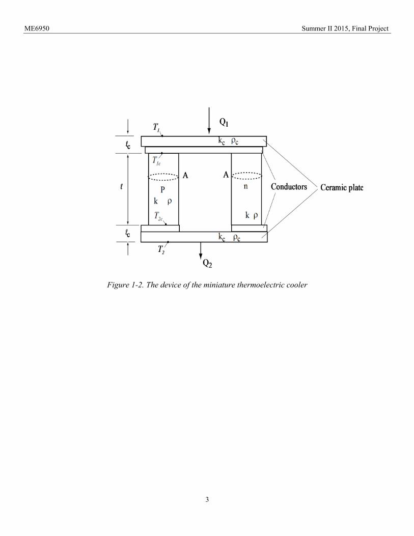
The figure 1-2 represents the miniature thermoelectric cooler that consists of three parts,

two ceramic plates, the layer conductors (copper) and two elements (P-type element and N-type

element). This project will focus on the contact resistance in the miniature thermoelectric

module farther progress in the development of short-legged thermoelectric micro modules for

cooling high power density electronic components. Theoretical analysis study is made to define

an available temperature lowering and maximum heat flux densities for short-legged coolers to

get high cooling power. When sort-long leg length is used, the materials properties (Seebeck

coefficient, figure of merit, thermal conductivity, and electrical conductivity) are difference if

the leg length is less than 0.5 mm.


3

Figure 1-2. The device of the miniature thermoelectric cooler


4

2. Mathematical formulation and modeling

2-1 Ideal equations including contact resistance

A simple thermoelectric cooling (TEC) is shown in Figure 1-2. The amount of heat absorbed

at the cold junction is associated with the Peltier cooling, the half of Joule heating including

contact resistance, and the thermal conduction. The basic equations used in this analytical are:

The cooling power is:

)(A

Q 11e

1 c

c

c TTl

k

(1)

)()I2

1-TIQ 11

2

1c1 c

o

e

e

c

e

o TTl

kA

AA

l

（ (2)

The amount of heat rejected from the hot plate is also obtained as shown in Figure (1):

)()I2

1TIQ 12c

2

2c2 c

o

e

e

c

e

o TTl

kA

AA

l

（ (3)

)(

AQ 22c

e2 TT

l

k

c

c

(4)


5

Where n p and np kk k ,k is the thermal conductivity of the thermoelements,

ck the thermal conduct conductivity which includes the thermal conductivity of ceramic plates

and the thermal conducts , l the thermoelement length, and cl the thickness of the contact

layer, is the electrical resistivity, Ae is cross-section area for the element, T2c and T1c are hot

and cold junction temperatures respectively, T1 and T2 are cold and hot side temperatures, lo is

leg length for element, and ρc represents the electrical resistivity.

2-2 Maximum Performance Parameters [2]:

The maximum performance parameters below are useful in math analytical. Equation (5) is

virtually the maximum current for the given material and geometry.

)1

)1

((I2

2

2

2m a xZ

TZ

TR

（5）

Or

R

TT )(*I m a x2

m a x

（6）

the maximum possible temperature difference is

2

2

2

22m a x T-Z

1T-

Z

1TT ）（）（（7）

Where Z is figure of merit.


6

the maximum possible cooling rate for the given material and geometry, we have

R

TTn

2

)(Q

2

m a x

2

2

2

c m a x （8）

The equations (5-8) are used in this project to create the equation that joins each of maximum

current, deferent temperature, and cooling power as a function of the leg length (lo).

2-3 Mathcad Analysis

The Mathcad software was used to make analytical way for the miniature thermoelectric

cooler. The analysis is made to describe the behavior of the cooling power and different

temperature with contact resistance and short leg length elements. The ideal equations including

the contact resistance are used in this project.

Figure 2-1. Cold side and cold junction temperature versus current


7

The figure 2-1 shows the relation between cold junction temperature and cold side

temperature with current supply [Appendix 1]. Where it is shown that the cold junction and

cold side temperature is the same with different current supply. When the current increased,

both the cold side and cold junction temperature were decreased to the current value equal to

3.8A at first and then increased.

In another hand, [Appendix 1] the hot junction temperature is increased when the current

supply is increased as that is shown in the figure 2-2.

Figure 2-2. Hot junction versus current supply


8

3. Effect material properties [2], [Appendix A]

The effective material properties are defined here as the material properties that are extracted

from the maximum parameters provided by the manufacturers or from measurements. The

effective figure of merit is obtained from Equation (9), which is

2

m a x2

m a x

)(

T2Z

TT

(9)

The effective Seebeck coefficient is obtained from Equation (6) and (8), which is

)(

Q2

m a x2m a x

m a x

TTIn

c

(10)

The effective electrical resistivity can be obtained using Equation (6), which is

m a x

m a x2 /)T-T

I

LAe

（

(11)

The effective thermal conductivity is now obtained, which is

Zk

2

(12)

By using the equation 9-12 as a function of thermoelement length（ ol ），where the figure 3-1


9

shows the effect leg length of element, it’s noted that the value of the figure of merit and

Seebeck coefficient are changed according to thermoelement length’s value in 0 mm to 0.5 mm,

in another hand, all the values of figure of merit and Seebeck coefficient have same value when

the leg length’s value is bigger than 0.5 mm.

Figure 3-1. Figure of merit and Seebeck coefficient versus leg length

In addition, the electrical resistivity and thermal conductivity take same way as figure of

merit and Seebeck coefficient. The figure 3-2 explains that the values of the electrical resistivity

and thermal conductivity are decreased because of the increased of the leg length’s value in

0mm to 0.5mm.


10

.

Figure 3-2. The electrical resistivity and thermal conductivity versus thermoelement length

Furthermore, the thermoelement is effective on the maximum cooling power and maximum

current as it is shown in figure 3-3. Where the decrease of the leg length leads to increasing the

maximum cooling power and maximum current. To be attention, When the value of the leg

length in 0.5 mm to 0 mm, the slop is prominent increased.

Figure 3-3. The maximum cooling power and maximum current versus thermoelement length


11

4. Literature validation and results comparing

4-1 Difference temperature

Maximum temperature difference versus leg length as it is shown in the figure 4-1, the solid

red line represents calculation by using ideal equation including contact resistance while the

dote points refers to experiment values by V. Semenyuk’s paper (2001) [1]. Where there is a

good agreement between calculation results and experiments results [Appendix A].

Figure 4-1. Calculation and experiment values versus leg length


12

4-2 Heat load characteristics of TE micro cooler

The figure 4-2 plots the variations of ∆T as a function of a heat load Qc at the cold side for

the AlN- module when different electrical currents are supplied. When ∆T is completely

suppressed the module demonstrates cooling power near 4.5 W which corresponds to heat flux

density of 75.6 W/cm2 at the cold junctions. Where the cross-section area of thermoelement is

0.41mm*0.41mm [Appendix B].

Figure 4-2. Heat load characteristics of TE micro cooler versus difference temperature


13

5. Cooling power and Geometry Factor

The figure 5-1 shows the cooling power versus the geometry factor with change in the

thermoelement length at different current supplied. Where the cooling power increases with

increasing the current supplied because of increasing in current leads to increasing in geometry

factor as that in the figure [Appendix B].

Figure 5-1. Cooling Power versus Geometry Factor


14

6. ANSYS Simulation

The thermoelectric cooler (one couple) has been simulated by using ANSYS program include

thermal-electric. It helped to make double sure to check fit with values which are obtained

analytically by using Mathcad software. The results are shown good agreement with it. The

simulation is made on two kinds of the thermoelectric cooler. The figure 6-1-A shows the

geometry of the first kind model which it is simulated. It consist of the two elements of the

material (ALN) with leg length (0.2mm) and cross-section (0.41mm*0.41mm) [1]. In addition,

the model has on two ceramic plates (0.62mm*0.41mm) one of them at top and another at

bottom. Furthermore, there is a layer of copper under each ceramic which has thickness

(0.03mm) with depth (0.41mm). While in the figure 6-1-B refers to second kind that has on two

ceramic plates with thickness (0.15mm) and a layer of copper with thickness (0.5mm).

Figure 6-1-A. Thermoelectric cooler with thickness (0.62 mm ceramic) and (0.03 mm copper)


15

Figure 6-1-B.

Geometry of the thermoelectric model with (0.15 mm ceramic) and (0.5 mm copper)

The main procedures that are applied to complete the simulation of the thermoelectric model

are:

6-1 Mesh

Mesh generation is one of the most critical aspects of engineering simulation. Too many cells

may result in long solver runs, and too few may lead to inaccurate results. ANSYS Meshing

technology provides a means to balance these requirements and obtain the right mesh for each

simulation in the most automated way possible. The figure 6-2-A explains the mesh for the first

kind of the thermoelectric cooler model (one couple) While figure 6-2-B shows the second kind

of the model.


16

Figure 6-2-A. Mesh of the first kind of the model

Figure 6-2-B. Mesh of the second kind of the model


17

6-2 Temperature Distribution

The first kind if the thermoelectric cooler model is shown in the figure 6-3-A. It shows

distribution the temperature from cold side to hot side. The cold side has junction cold

temperature about 242.161 K and junction hot has temperature about (304.6 K) with current

supply (2 Amber). As it is shown in the figure, the distribution starts of the cold to hot side.

While the figure 6-3-B explains second kind, where the junction cold temperature is about

(263.4K) and hot junction temperature is about (303.225K).

Figure 6-3-A. Temperature Distribution


18

Figure 6-3-B. Temperature Distribution

6-3 Current Distribution

The final step in this simulation is form distribute the current when it supplied through the

thermoelectric. In the figure 6-4-A, it is shown current distribution of right side to left side that

has value (2 Amber) for first kind and figure 6-4-B shows second kind.

Figure 6-4-A. Current Distribution


19

Figure 6-4-B. Current Distribution

7. Results and Discussion

The change in value of current supply and thickness of the ceramic and copper effect on the

junction temperatures and heat flow. Where the increasing in supplying the current leads to

increase in the junction temperatures (cold and hot) and heat flux. In addition, this increasing

leads to increasing in error percentage between results that are obtained from Mathcad software

and ANSYS program. While the increasing copper thickness also effects on the results, where

when the copper has increasing in the thickness, the values of junction cold and hot

temperatures becomes close to values that are obtained of Mathcad software with decries the

ceramic thickness. Below the compare between the values obtained of the ANSYS simulation

for two kinds and Mathcad calculations.


20

8. Conclusion

The short thermoelement length less than 0.5 mm for thermoelectric cooler has effect on each

of cooling power, and effective materials. Mathematically analysis study are made to define an

available temperature lowering and maximum heat flux densities for short-legged coolers by

using ideal equations which including contact resistance. The temperature differences is about

71K are obtained with TE leg lengths down to 0.2 mm. In addition, the project has a validation

for ‘Thermoelectric Micro Modules for Spot Cooling of High Density Heat Sources’ [1]. Where

this validation includes two main important things, difference temperature as a function of the

cooling power and the maximum difference temperature with thermoelement length. The

prediction which is obtained from equations as a validation has a good agreement with

experiment work by V. Semenyuk. Finally, ANSYS simulation has improved great matching

with the prediction results.


21

References

[1] - Semenyuk, V. ‘Thermoelectric Micro Modules for Spot Cooling of High Density Heat

Sources.’ Proceedings ICT2001.20 International Conference on thermoelectric.

[2]- Lee, HoSung, Attar, Alaa, Weera, Sean, Performance Prediction of Commercial

Thermoelectric Cooler Modules using the Effective Material Properties, Journal of Electronic

Materials, Vol.44, No.6, 2157-2165 (2015).

[3] Huang, B.j, C.j Chin, and C.l Duang. "A Design Method of Thermoelectric Cooler." International

Journal of Refrigeration 23.3 (2000): 208-18. Web.

[4] Chen, Wei-Hsin, Chen-Yeh Liao, and Chen-I Hung. "A Numerical Study on the Performance of

Miniature Thermoelectric Cooler Affected by Thomson Effect." Applied Energy 89.1 (2012): 464-73.

Web

http://homepages.wmich.edu/~leehs/ME695/Effective%20material%20properties%20paper.pdf



contact resistances for miniature thermoelectric devices

Documents