contagion and trade: why are currency crises regional...

Contagion and Trade: Why Are Currency Crises Regional?Reuven Glick and Andrew K. Rose*

Revised Draft: August 12, 1998Comments Welcome

AbstractCurrency crises tend to be regional; they affect countries in geographic proximity. This suggeststhat patterns of international trade are important in understanding how currency crises spread,above and beyond any macroeconomic phenomena. We provide empirical support for thishypothesis. Using data for five different currency crises (in 1971, 1973, 1992, 1994, and 1997)we show that currency crises affect clusters of countries tied together by international trade. Byway of contrast, macroeconomic and financial influences are not closely associated with thecross-country incidence of speculative attacks. We also show that trade linkages help explaincross-country correlations in exchange market pressure during crisis episodes, even aftercontrolling for macroeconomic factors.

Keywords: speculative; attack; exchange rates; reserve; international; macroeconomic;empirical; financial.

JEL Classification Number: F32.

Reuven Glick Andrew K. RoseFederal Reserve Bank of San Francisco Haas School of Business101 Market St., University of CaliforniaSan Francisco CA 94105 Berkeley, CA USA 94720-1900Tel: (415) 974-3184 Tel: (510) 642-6609Fax: (415) 974-2168 Fax: (510) 642-4700E-mail: [email protected] E-mail: [email protected]

* Glick is Vice President and Director of the Center for Pacific Basin Studies, EconomicResearch Department, Federal Reserve Bank of San Francisco. Rose is Professor of EconomicAnalysis and Policy in the Haas School of Business at the University of California, Berkeley, actingdirector of the NBER International Finance and Macroeconomics program, and CEPR ResearchFellow. We thank Priya Ghosh and Laura Haworth for research assistance. For comments, wethank the participants of the CEPR/World Bank Conference “Financial Crises: Contagion andMarket Volatility,” Joshua Aizenman, Gabriele Galati, Marcus Miller, Richard Portes, JavierSuárez, Mark Taylor, and especially David Vines. The views expressed below do not representthose of the Federal Reserve Bank of San Francisco or the Board of Governors of the FederalReserve System, or their staffs. A current (PDF) version of this paper and the (Excel 97spreadsheet) data set used in the paper are available at http://haas.berkeley.edu/~arose.

1

I: Introduction

Currency crises tend to be regional. In this paper, we attempt to document this fact, and

to understand its implications.

Most economists think about currency crises using one of two standard models of

speculative attacks. The “first generation” models of, e.g., Krugman (1979) direct attention to

inconsistencies between an exchange rate commitment and domestic economic fundamentals

such as an underlying excess creation of domestic credit, typically prompted by a fiscal

imbalance. The “second generation” model of, e.g., Obstfeld (1986) views currency crises as

shifts between different monetary policy equilibria in response to self-fulfilling speculative

attacks. There are many variants of both models, and a number of empirical issues associated

with both classes of models, as discussed in Eichengreen, Rose and Wyplosz (1995). What is

common to both classes of models is their emphasis on macroeconomic and financial

fundamentals as determinants of currency crises. But macroeconomic phenomena do not tend to

be regional. Thus, from the perspective of most speculative attack models, it is hard to

understand why currency crises tend to be regional, at least without an extra ingredient

explaining why the relevant macro fundamentals are intra-regionally correlated.1

On the other hand, trade patterns are regional; countries tend to export and import with

countries in geographic proximity.2 Prima facie then, trade linkages seem like an obvious place

to look for a regional explanation of currency crises. It is easy to imagine why the trade channel

might potentially be important. If prices tend to be sticky, a nominal devaluation delivers a real

exchange rate pricing advantage, at least in the short run. That is, countries lose competitiveness

when their trading partners devalue. They are therefore more likely to be attacked — and to

devalue — themselves.

2

Of course, this channel may not be important in practice. Nominal devaluations need not

result in real exchange rate changes for any long period of time. Devaluations are costly and can

be resisted. Making the case for the trade channel is primarily an empirical exercise.

This paper is intended to contribute a single point to the growing literature on currency

contagion. We argue that trade is an important channel for contagion, above and beyond

macroeconomic influences. Countries who trade and compete with the targets of speculative

attacks are themselves likely to be attacked.

Our point is modest and intuitive. We ignore a number of related issues. For instance, in

trying to model “contagion” in currency crises, we do not rule out the possibility of (regional)

shocks common to a number of countries. Moreover, we do not attempt to study the timing of

currency crises. We do intend to show that, given the occurrence of a currency crisis, the

incidence of speculative attacks across countries is linked to the importance of international trade

linkages. That is, currency crises spread along the lines of trade linkages, after accounting for

the effects of macroeconomic and financial factors.3 This linkage is intuitive, economically

significant, statistically robust, and important in understanding the regional nature of speculative

attacks.

Section II motivates the analysis by discussing the regional nature of three recent waves

of speculative attacks. This is followed by a section that provides a framework for our analysis.

Our methodology and data are discussed in section IV; the actual empirical results follow. The

paper ends with a brief conclusion.

II: Have Currency Crises Been Regional?

Substantially. But not exclusively.

3

The last decade has witnessed three important currency crises. In the autumn of 1992, a

wave of speculative attacks hit the European Monetary System and its periphery. Before the end

of the year, five countries (Finland, the UK, Italy, Sweden and Norway) had floated their

currencies. Despite attempts by a number of countries to remain in the EMS with the assistance

of devaluations (by Spain, Portugal and Ireland), the system was unsalvageable. The bands of

the EMS were widened to ± 15% in August 1993. Eichengreen and Wyplosz (1993) provide a

well-known review of the EMS crisis.

The Mexican peso was attacked in late 1994 and floated shortly after an unsuccessful

devaluation. Speculative attacks on other Latin American countries occurred immediately. The

most prominent targets of the “Tequila Hangover” were Latin American countries, especially

Argentina and Brazil, but also including Peru and Venezuela. Not all Latin countries were

attacked — Chile being the most visible exception — and not all economies attacked were in

Latin America (Thailand, Hong Kong, the Philippines and Hungary also suffered speculative

attacks). While there were few devaluations, the attacks were not without effect. Argentine

macroeconomic policy in particular tightened dramatically, precipitating a sharp recession.

Sachs, Tornell and Velasco (1996) provide one of many summaries of the Mexican crisis and its

aftermath.

The “Asian Flu” began with continued attacks on Thailand in the late spring of 1997 and

continuing with flotation of the baht in early July 1997. Within days speculators had attacked

Malaysia, the Philippines, and Indonesia. Hong Kong and Korea were attacked somewhat later

on; the crisis then spread across the Pacific to Chile and Brazil. The effects of “Bhatulism”

linger on as this paper is being written; Corsetti, Pesenti and Roubini (1998) provide an

exhaustive survey.

4

All three waves of attacks were largely regional phenomena.4 Once a country had

suffered a speculative attack – Thailand in 1997, Mexico in 1994, Finland in 1992 – its trading

partners and competitors were disproportionately likely to be attacked themselves. Not all major

trading partners devalued – indeed, not all major trading partners were even attacked.

Macroeconomic and financial influences are certainly not irrelevant. But neither, as we shall

see, is the trade channel irrelevant as a means of transmitting speculative pressures across

international borders.

III: The Framework

Contagion in currency crises has come to be studied by economists only recently.

Eichengreen, Rose and Wyplosz (1996) provide a critical survey and some early evidence.

For the purposes of this study, we think of a currency crisis as being contagious if it

spreads from the initial target(s), for whatever reason. As is well known, it is difficult to

distinguish empirically between common shocks and contagion. The evidence in favor of

contagion is indirect at best. Still, we believe that the preponderance of evidence favors the

existence of contagion effects; Eichengreen and Rose (1998) provide evidence.

There are at least two different types of explanations for why contagion spreads,

transmission mechanisms that are not mutually exclusive. The first relies on macroeconomic or

financial similarity. A crisis may spread from the initial target to another if the two countries

share various economic features. The work of Sachs, Tornell and Velasco (1996) can be viewed

in this light. Sachs et. al. focus on three intuitively reasonable fundamentals: real exchange rate

over-valuation; weakness in the banking system; and low international reserves (relative to broad

money). They find that their three variables can explain half the cross-country variation in a

5

crisis index, itself a weighted average of exchange rate depreciation and reserve losses. They use

data for twenty developing countries in late 1994 and early 1995. Similarly, similarity in terms

of structural characteristics of the economy is analyzed in Rigobon (1998). Currency crises may

be regional if macroeconomic features of economies tend to be regional.

The alternative view is that a devaluation gives a country a temporary boost in its

competitiveness, in the presence of nominal rigidities. Its trade competitors are then at a

competitive disadvantage; those most adversely affected by the devaluation are likely to be

attacked next. Gerlach and Smets (1994) formalize this reasoning; Huh and Kasa (1997) provide

related analysis. In this way, a currency crisis that hits one country (for whatever reason) may be

expected to spread to its trading partners. Since trade patterns are strongly negatively affected by

distance, currency crises will tend to be regional.

Eichengreen and Rose (1998) found both “macroeconomic” and “trade” channels of

transmission to be empirically relevant in a large quarterly panel of post-1959 industrial country

data; trade effects dominated. Thus it is not clear a priori which of the mechanisms for

contagion, if any, might be present in the data we examine. For this reason, we try to account for

both in our empirical work.

IV: Methodology

Our objective in this paper is to demonstrate that trade provides an important channel for

contagion above and beyond macroeconomic and financial similarities. As a result, we focus on

the incidence of currency crises across countries. We ask why some countries are hit during

certain episodes of currency instability, while others are not.

6

Empirical Strategy

Our strategy keys off the “first victim” of a speculative attack. A country is attacked for

some reason. We do not take a stance one way or another on whether this initial attack is

warranted by bad fundamentals (as would be true in a first-generation model) or is the result of a

self-fulfilling attack (consistent with a second-generation model). Instead, we ask: “Given the

incidence of the initial attack, how does the crisis spread out from “ground zero?” Are the

subsequent targets closely linked by international trade to the first victim? Do they share

common macroeconomic similarities? We interpret evidence in favor of the first hypothesis as

indicating the importance of the trade channel of contagion.

Clearly we do not deal with a number of related and important issues. We assume that

there is contagion, and do not test for its presence. We do not attempt to explain the timing of

currency crises. Finally, we do not ask why some crises become contagious and spread while

others do not.

Our regression framework is of the form:

Crisisi = ϕTradei + λMi + εi

where: Crisisi is an indicator variable which is initially defined as unity if country i was attacked

in a given episode, and zero if the country was not attacked; Mi is a set of macroeconomic

control regressors; λ is the corresponding vector of nuisance coefficients; and ε is a normally

distributed disturbance representing a host of omitted influences which affect the probability of a

currency crisis.

7

We estimate this binary probit equation across countries via maximum likelihood. The

null hypothesis of interest is Ho: ϕ=0. We interpret evidence against the null as being consistent

with a trade contagion effect.

We also use a different set of regressands, exploring more quantitative crisis indicators.

When the regressand is a continuous indicator of “exchange market pressure”, we estimate this

cross-country equation by OLS. In this case we consider not just the significance of ϕ, but also

its sign.

The Data Set

We use cross-sectional data from five different episodes of important and widespread

currency instability. These are: 1) the breakdown of the Bretton Woods system in the Spring of

1971; 2) the collapse of the Smithsonian Agreement in the late Winter of 1973; 3) the EMS

Crisis of 1992-93; 4) the Mexican meltdown and the Tequila Effect of 1994-95; and 5) the Asian

Flu of 1997-98. Our data set includes data from 161 countries, many of which were directly

involved in none of the five episodes.5

Making our work operational entails: a) measuring currency crises; b) measuring the

importance of trade between the “first victim” and country i; and c) measuring the relevant

macroeconomic and financial control variables. We now deal with these tasks in order.

Currency Crises

To construct our simple binary indicator regressand, it is relatively easy to determine

crisis victims from journalistic and academic histories of the various episodes (we rely on The

Financial Times in particular). Our list of crisis countries is included in appendix table A1.

8

Table A1 also lists the “first victim” or “ground zero” countries first attacked. For some

periods the “first victim” is relatively straightforward (Mexico in 1994, Thailand in 1997). For

others, it is more arguable. In 1971 and 1973 we consider Germany to be ground zero. A case

can be made that the U.S. should be ground 0 for the 1971 and 1973 episodes. However, since

the U.S. dollar was the key currency of the international monetary system, the change in the

value of the dollar during these periods can be interpreted more as a common shock. A priori,

we choose to rule out such a common shock when testing for contagion effects transmitted

through the trade channel. The 1992 crisis is more complex still. We think of the Finnish

flotation as being the first important incident (making Finland “ground zero”), but one can make

a case for Italy (which began to depreciate immediately following the Danish Referendum) or

Germany because of the aftermath of Unification (though as the center of the EMS, German

shocks are common). As we shall see, our probit results do not appear to be very sensitive to the

exact choice of “first victim” country.

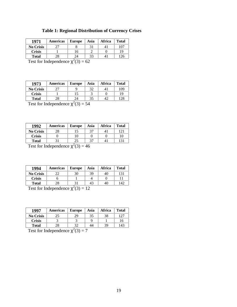
The five waves of currency crises we examine all appear to have a strongly regional

nature. Table 1 is a series of cross-tabulations of currency crises and non-crises in our five

episodes by regions. The chi-squared tests of independence confirm what the eye can see,

namely that currency crises appear to be regional.

Trade Linkages

Once our “ground zero” country has been chosen, we need to be able to quantify the

importance of international trade links between the first victim and other countries. We focus on

the degree to which the two countries compete in third markets. Our default measure of trade

linkage is

9

Tradei ≡ Σk {[(x0k + xik)/(x0. + xi.)] · [1 − |(xik − x0k)|/(xik + x0k]}

where xik denotes aggregate bilateral exports from country i to k (k ≠ i, 0) and xi. denotes

aggregate bilateral exports from country i. This index is a weighted average of the importance of

exports to country k for countries 0 and i. The importance of country k is greatest when it is an

export market of equal importance to both 0 and i. The weights are proportional to the

importance of country k in the aggregate trade of countries 0 and i. The top twenty trade

partners linked to “ground zero” are tabulated in Table A2.6

This is clearly an imperfect measure of the importance of trade linkages between country

i and “ground zero.” It relies on actual rather than potential trade. It ignores direct trade

between the two countries. Imports are ignored. Countries of vastly different size are a potential

problem. Cascading effects are ignored.7

We have computed a number of different perturbations to our benchmark measure, and

found that our trade measures are relatively insensitive to the exact way we measure the trade

linkage. For instance, we have calculated a “direct” measure of trade and a “total” measure of

trade. Our direct trade measure is defined analogously to our benchmark measure as

DirectTradei = 1 − |xi0 − x0i|/(xi0 + x0i).

This index is higher the more equal are bilateral exports between countries 0 and i. A measure of

total trade, TotalTradei, is the weighted sum of Tradei and DirectTradei, where the latter is

10

weighted by (xi0 + x0i)/(x0. + xi.). We have also used a measure of trade linkages which uses

trade shares, so as to adjust for the varying size of countries:

TradeSharei ≡ Σk{[(x0k + xik)/(x0. + xi.)] ·

[ 1 − |{(x0k/x0.) − (xik/xi.)}|/{(x0k/x0.) + (xik/xi.)}]}

We check extensively for the sensitivity our results to ensure that our results do not depend on

the exact measure of trade linkage.

We computed our trade measures for our different episodes using annual data for the

relevant crisis year taken from the IMF’s Direction of Trade data set.8,9 The rankings of the top

twenty trade competitors of the “first victim” are tabulated (by ranking of “Trade”) in an

appendix table, and seem sensible. For instance, the most important export competitors for

Finland are Norway and Denmark. But some of the competitors are not intuitive. For instance,

some countries enter the rankings that are probably not direct trade competitors (e.g., OPEC

countries); this is an artifact of the aggregate nature of our data.

Macroeconomic Controls

Our objective is to use a variety of different macroeconomic controls to account for the

standard determinants of currency crises dictated by first- and second-generation models. We do

this so that our trade linkage variable picks up the effects of currency crises abroad that spill over

because of trade; that is, after taking account of macroeconomic and financial imbalances that

might lead to a currency crisis. Our most important controls are: the annual growth rate of

domestic credit (IFS line 32); the government budget as a percentage of GDP (a surplus being

11

positive; IFS line 80 over line 99b); the current account as a percentage of GDP (IFS line 78ald

multiplied by line rf in the numerator); the growth rate of real GDP (IFS line 99b.r); the ratio of

M2 to international reserves (IFS lines 34+35 multiplied by line rf over line1l.d); and domestic

CPI inflation (IFS line 64); and the degree of currency under-valuation. We measure the latter

by constructing an annual real exchange rate index as a weighted sum of bilateral real exchange

rates (using domestic and real CPIs) in relation to the currencies of all trading partners with

available data. The weights sum to one and are proportional to the bilateral export shares with

each partner. The degree of currency under-valuation is defined as the percentage change in the

real exchange rate index between the average of the three prior years and the episode year. A

positive value indicates that the real exchange rate is depreciated relative to the average of the

three previous years.10

Our data is annual, and was extracted from the IMF’s International Financial Statistics.11

It has been checked for outliers via both visual and statistical filters.

V: Some Results

Univariate Evidence on Trade and Macroeconomic Linkages

Table 2 is a series of t-tests that test for equality of cross-country means for countries

affected and unaffected by currency crises. These are computed under the null hypothesis of

equality of means between crisis and non-crisis countries (assuming equal but unknown

variances). Thus, a significant difference in the behavior of the variable across crisis and non-

crisis countries – for instance consistently higher money growth for crisis countries – would

show up as a large (negative) t-statistic.

12

There are two important messages from Table 2. First, the strength of trade linkage to

“ground zero” varies systematically between crisis and non-crisis countries. In particular, it is

systematically higher for crisis countries at reasonable levels of statistical significance. Second,

macroeconomic variables do not typically vary systematically across crisis and non-crisis

countries. While some variables sometimes have significantly different means, these results are

not consistent across episodes. And they are never as striking as the trade results. These

findings are consistent with the importance of the trade channel in contagion.

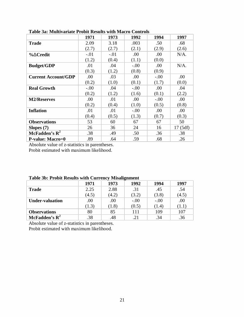
Multivariate Probit Results for Binary Crisis Measure

Table 2 is not completely persuasive. One problem is that it consists of a set of univariate

tests. We remedy that problem in Table 3. The top panel of Table 3 is a multivariate equivalent

of Table 2, including a host of macroeconomic variables simultaneously with the trade variable.

It reports probit estimates of cross-country crisis incidence on trade linkage and macroeconomic

controls. The latter variables are dictated by a variety of different models of speculative attacks

(as discussed in Eichengreen, Rose and Wyplosz (1995)) which can be viewed as primitive

determinants of vulnerability to speculative pressure. Table 3b uses a wider range of countries

(since many macroeconomic observations are missing in our sample) but restricts attention to the

degree of currency under- or over-valuation. This is viewed by some as a summary statistic for

macroeconomic misalignment.

Since probit coefficients are not easily interpretable, we report the effects of one-unit

(i.e., one percentage point) changes in the regressors on the probability of a crisis (also expressed

in probability values so that .01=1%), evaluated at the mean of the data. We include the

associated z-statistics in parentheses; these test the null of no effect variable by variable.

13

Diagnostics are reported at the foot of the table. These include a test for the joint significance of

all the coefficients (“Slopes”) which is distributed as chi-squared with seven degrees of freedom

under the null hypothesis of no effect. We also include a p-value for the hypothesis that none of

the macro effects are jointly significant (i.e., all the coefficients except the trade effect).

The results are striking. The trade channel for contagion seems consistently important in

both statistical and economic terms. While the economic size of the effect varies significantly

across episode it is consistently different from zero at conventional levels of statistical

significance. Its consistently positive sign indicates that a stronger trade linkage is associated

with a higher incidence of a currency crisis.

On the other hand, the macroeconomic controls are small economically and rarely of

statistical importance. This is true both of individual variables, of all seven macroeconomic

factors taken simultaneously, and of currency under-valuation.

Succinctly, the hypothesis of no significant trade channel for contagion seems wildly

inconsistent with the data, while macroeconomic controls do not explain the cross-country

incidence of currency crises.

Robustness

We have checked for the sensitivity of our probit results with respect to a number of

perturbations to our basic methodology. A number of robustness checks are exhibited in the

three different panels of Table 4.

The first part of Table 4 varies the macro control regressors. In place of the

macroeconomic regressors of Table 3, we substitute: the growth rate of M1 (IFS line 34); the

change in the budget/GDP and current account/GDP ratios; and the investment/GDP ratio (IFS

14

93e over line 99b). We also add the country credit rating from Institutional Investor.12 However

our trade linkage variable remains positive and statistically significant despite our substitutions.

We have also tried a variety of other sets of macroeconomic controls, without changing the thrust

of our results; for the sake of brevity, these experiments are not reported.

The second panel in Table 4 leaves the macro controls unchanged (and unreported, again

for the sake of compactness) and substitutes different measures of trade linkages between the

country and “ground zero.” We use: the rank rather than the actual continuous measure of

Tradei (with a rank of “1” denoting the most important trading partner, “2” being the second

more important trade linkage and so forth), our measure of total trade, and our measure of trade

share linkages. Our finding of a positive statistically significant role for trade linkages is not

substantially altered.

We have also changed the regressand, that is, the way we measure the actual incidence of

crises across countries. Results are reported in Table 4c. The first row shows the effect of

treating the United States as “ground zero” in 1971 and 1973; the second and third rows use

Germany and Italy respectively as “ground zero” in 1992. Our finding of a significant trade

effect is not destroyed by using other (reasonable) starting points for these contagion episodes.

Corsetti et. al. (1998) and Tornell (1998) use cross-sectional techniques and data similar

to ours to examine the incidence of the Asian crisis; Tornell also considers the 1994-95 Tequila

attacks. We have reproduced the results of both studies, using their own data. When we added

our trade variable to the default Tornell regression (which explains crisis severity with a pooled

data set from 1994 and 1997), it is correctly signed and significant at the .02 level. When we

added our trade variable to the default Corsetti et. al. regression, our benchmark trade variable is

again correctly signed and significant at better than the .01 level. The robustness of our key

15

result – the important role played by trade linkages even after taking into account

macroeconomic effects – is quite reassuring.

OLS Results for Continuous Crisis Measures

In the previous section we showed that our measure of trade competition worked well in

explaining the incidence of currency crises defined in terms of a simple binary indicator. In this

section we seek to explain both the direction and magnitude of a quantitative index of exchange

market pressure during crisis episodes.13

We employ two continuous measures of exchange market pressure. The first measure is

the cumulative percent change in the nominal devaluation rate with respect to the ground zero

currency for six months following the occurrence of a crisis.14 The second measure is a

weighted average of the devaluation rate and the percent decline in international reserves for six

months following the crises. (We check for robustness by also examining three- and nine-month

horizons). Following others (Eichengreen, Rose, and Wyplosz (1995, 1996); Frankel and Rose

(1996) and Sachs, Tornell and Velasco, 1996), we weight the components so as to equalize their

volatilities; that is, we weight each component by the inverse of its variance over the sum of

inverses of the variances, where the variances are calculated using three years of monthly data

prior to each episode. This weighting scheme gives a larger weight to the component with a

smaller variance.

Our continuous measures of exchange rate crises are not without their limitations. First,

countries that successfully defend themselves against speculative attacks may show no sign of

attack by experiencing either an exchange rate depreciation or reserve losses. A somewhat

broader measure of possible responses to speculative attacks would include the interest rate.

16

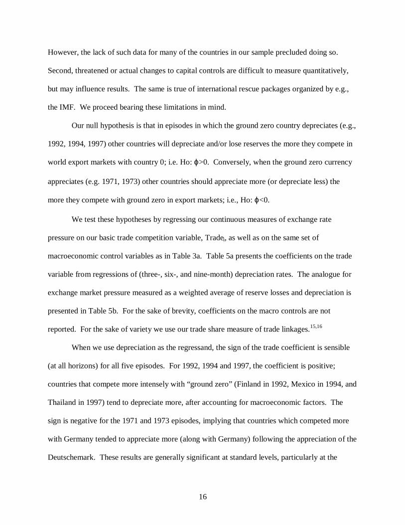
However, the lack of such data for many of the countries in our sample precluded doing so.

Second, threatened or actual changes to capital controls are difficult to measure quantitatively,

but may influence results. The same is true of international rescue packages organized by e.g.,

the IMF. We proceed bearing these limitations in mind.

Our null hypothesis is that in episodes in which the ground zero country depreciates (e.g.,

1992, 1994, 1997) other countries will depreciate and/or lose reserves the more they compete in

world export markets with country 0; i.e. Ho: ϕ>0. Conversely, when the ground zero currency

appreciates (e.g. 1971, 1973) other countries should appreciate more (or depreciate less) the

more they compete with ground zero in export markets; i.e., Ho: ϕ<0.

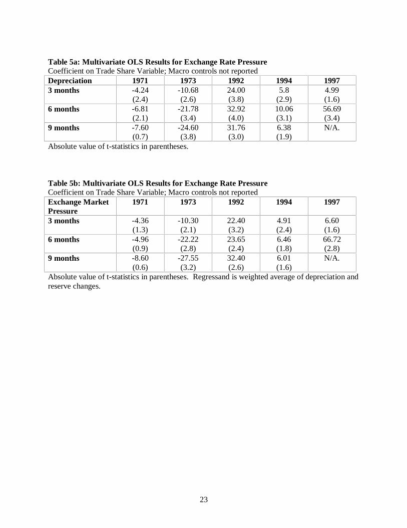
We test these hypotheses by regressing our continuous measures of exchange rate

pressure on our basic trade competition variable, Tradei, as well as on the same set of

macroeconomic control variables as in Table 3a. Table 5a presents the coefficients on the trade

variable from regressions of (three-, six-, and nine-month) depreciation rates. The analogue for

exchange market pressure measured as a weighted average of reserve losses and depreciation is

presented in Table 5b. For the sake of brevity, coefficients on the macro controls are not

reported. For the sake of variety we use our trade share measure of trade linkages.15,16

When we use depreciation as the regressand, the sign of the trade coefficient is sensible

(at all horizons) for all five episodes. For 1992, 1994 and 1997, the coefficient is positive;

countries that compete more intensely with “ground zero” (Finland in 1992, Mexico in 1994, and

Thailand in 1997) tend to depreciate more, after accounting for macroeconomic factors. The

sign is negative for the 1971 and 1973 episodes, implying that countries which competed more

with Germany tended to appreciate more (along with Germany) following the appreciation of the

Deutschemark. These results are generally significant at standard levels, particularly at the

17

longer horizons. When we consider exchange market pressure – the weighted average of

depreciation and reserve losses – as the crisis measure, the overall results for the six and nine

month horizons are similar, though the significance level generally declines.17

Tables 6a and 6b report the complete results for the six-month horizon for depreciation

and exchange market pressure respectively. Only inflation is generally significant across all

episodes aside from inflation. In contrast, as noted above with our cumulative depreciation

measure as the regressand, the trade variable appears to provide consistent explanatory power for

all crisis episodes.18

We conclude that our continuous quantitative indicators, particularly the cumulative

deprecation rate, provide support for the hypothesis that trade contributes significant power in

explaining the magnitude as well as incidence of currency crises.

VI: Concluding Comments

We have found strong evidence that currency crises tend to spread along regional lines

using both binary and more continuous measures of crises. This is true of five recent waves of

speculative attacks (in 1971, 1973, 1992, 1994-95, and 1997). Accounting for a variety of

different macroeconomic effects does not change this result. Indeed macroeconomic factors do

not consistently help much in explaining the cross-country incidence of speculative attacks.

Our evidence is consistent with the hypothesis that currency crises spread because of

trade linkages. That is, countries may be attacked because of the actions (or inaction) of their

neighbors, who tend to be trading partners merely because of geographic proximity. This

externality has important implications for policy. If this effect exists, it is a strong argument for

18

international monitoring. A lower threshold for international and/or regional assistance is also

warranted than would be the case if speculative attacks were solely the result of domestic factors.

19

Table 1: Regional Distribution of Currency Crises

1971 Americas Europe Asia Africa Total

No Crisis 27 8 31 41 107Crisis 1 16 2 0 19Total 28 24 33 41 126

Test for Independence χ2(3) = 62




1992 Americas Europe Asia Africa TotalNo Crisis 28 15 37 41 121

Crisis 0 10 0 0 10Total 31 25 37 41 131








20

Table 2: T-Tests for Equality by Crisis Incidence

1971 1973 1992 1994 1997Trade -9.5 -10.9 -4.7 -6.9 -7.5%∆M1 .8 1.1 1.2 -.9 -.1%∆M2 1.6 .8 1.1 -.6 .0%∆Credit .8 1.3 .4 -.2 -.4%∆Private Credit 1.2 .1 .7 -.5 .3M2/Reserves -3.5 -2.6 .3 .5 -.3%∆Reserves -1.8 .7 1.3 1.4 2.1%∆Exports -1.0 -.9 .1 -.5 .1%∆Imports -1.5 -1.1 .8 -1.1 -.6Current Account/GDP -2.0 -2.1 -.8 .2 -.8Budget/GDP -1.6 -1.9 1.4 -.9 -.4Real Growth .7 .5 1.1 -1.6 -2.7Investment/GDP -3.2 -2.8 1.0 -.2 -2.7Inflation -.3 .7 1.5 -1.0 .6Under-valuation -.5 -.9 .6 1.5 -.6

Values tabulated are t-statistics, calculated under the null hypothesis of equal means andvariances. A significant negative statistic indicates that the variable was significantly higher forcrisis countries than for non-crisis countries.

21

Table 3a: Multivariate Probit Results with Macro Controls1971 1973 1992 1994 1997

Trade 2.09(2.7)

3.18(2.7)

.003(2.1)

.50(2.9)

.68(2.6)

%∆Credit -.01(1.2)

-.01(0.4)

.00(1.1)

.00(0.0)

N/A.

Budget/GDP .01(0.3)

.04(1.2)

-.00(0.8)

.00(0.9)

N/A.

Current Account/GDP .00(0.2)

.03(1.0)

.00(0.1)

-.00(1.7)

.00(0.0)

Real Growth -.00(0.2)

.04(1.2)

-.00(1.6)

.00(0.1)

.04(2.2)

M2/Reserves .00(0.2)

.01(0.4)

.00(1.0)

-.00(0.5)

.00(0.8)

Inflation .01(0.4)

.01(0.5)

-.00(1.3)

.00(0.7)

.00(0.3)

Observations 53 60 67 67 50Slopes (7) 26 36 24 16 17 (5df)McFadden’s R2 .38 .49 .50 .36 .38P-value: Macro=0 .89 .64 .59 .68 .26Absolute value of z-statistics in parentheses.Probit estimated with maximum likelihood.

Table 3b: Probit Results with Currency Misalignment1971 1973 1992 1994 1997

Trade 2.25(4.5)

2.88(4.2)

.31(3.2)

.45(3.8)

.54(4.5)

Under-valuation .00(1.3)

.00(1.8)

-.00(0.5)

-.00(1.4)

.00(1.1)

Observations 80 85 111 109 107McFadden’s R2 .38 .48 .21 .34 .36Absolute value of z-statistics in parentheses.Probit estimated with maximum likelihood.

22

Table 4a: Sensitivity Analysis: Macro Controls1971 1973 1992 1994 1997

Trade 1.28(2.6)

1.21(3.1)

.002(1.6)

.0002(2.1)

.23(1.6)

%∆M1 -.01(1.3)

-.00(0.6)

-.00(1.1)

-.00(.6)

-.00(.9)

∆ (Budget/GDP) .03(0.7)

-.01(0.9)

.00(.4)

.00(1.0)

-.01(.8)

∆ (CurrentAccount/GDP)

.01(0.9)

-.01(1.2)

.00(1.2)

-.00(.4)

-.00(.7)

Investment/GDP .02(1.8)

.02(2.0)

-.00(1.0)

.00(1.1)

.00(.7)

Institutional InvestorRating

N/A. N/A. .00(1.4)

-.000001(1.8)

-.00(.8)

Observations 54 60 62 63 27Slopes (df) 26 (5) 38 (5) 24 (6) 24 (6) 13 (6)McFadden’s R2 .41 .59 .61 .62 .58P-value: Macro=0 .25 .40 .60 .71 .67Absolute value of z-statistics in parentheses. Probit estimated with maximum likelihood.

Table 4b: Sensitivity Analysis: Trade MeasureCoefficients on Trade Variable; Macro Controls (from Table 3a) not reported

1971 1973 1992 1994 1997Rank of Trade -.01

(3.3)-.01(3.1)

-.00(1.9)

-.001(1.9)

-.003(2.1)

Total Trade 2.05(2.7)

3.15(2.7)

.004(2.2)

.51(2.9)

.68(2.7)

Trade Share 1.54(3.5)

2.04(3.3)

.000(1.8)

.23(2.2)

.57(2.1)

Absolute value of z-statistics in parentheses. Probit estimated with maximum likelihood.

Table 4c: Sensitivity Analysis: RegressandCoefficients on Trade Variable; Macro Controls not reported“Ground Zero” 1971 1973 1992U.S. 1.39

(2.1)1.85(2.6)

N/A.

Germany N/A. N/A. .95(3.0)

Italy N/A. N/A. .46(3.0)

Absolute z-statistics in parentheses. MLE Probit.

23

Table 5a: Multivariate OLS Results for Exchange Rate PressureCoefficient on Trade Share Variable; Macro controls not reportedDepreciation 1971 1973 1992 1994 19973 months -4.24

(2.4)-10.68(2.6)

24.00(3.8)

5.8(2.9)

4.99(1.6)

6 months -6.81(2.1)

-21.78(3.4)

32.92(4.0)

10.06(3.1)

56.69(3.4)

9 months -7.60(0.7)

-24.60(3.8)

31.76(3.0)

6.38(1.9)

N/A.

Absolute value of t-statistics in parentheses.

Table 5b: Multivariate OLS Results for Exchange Rate PressureCoefficient on Trade Share Variable; Macro controls not reportedExchange MarketPressure

1971 1973 1992 1994 1997

3 months -4.36(1.3)

-10.30(2.1)

22.40(3.2)

4.91(2.4)

6.60(1.6)

6 months -4.96(0.9)

-22.22(2.8)

23.65(2.4)

6.46(1.8)

66.72(2.8)

9 months -8.60(0.6)

-27.55(3.2)

32.40(2.6)

6.01(1.6)

N/A.

Absolute value of t-statistics in parentheses. Regressand is weighted average of depreciation andreserve changes.

24

Table 6: Multivariate OLS Results for Exchange Rate Pressure: 6 month HorizonDepreciation 1971 1973 1992 1994 1997Trade Share -6.81

(2.1)-21.78(3.4)

32.92(4.0)

10.06(3.1)

56.69(3.4)

%∆Credit 0.02(0.3)

-0.01(0.1)

0.01(1.1)

0.05(2.0)

-0.09(0.7)

Budget/GDP -0.42(2.7)

-0.68(2.3)

-0.24(0.7)

-0.04(0.6)

-1.63(1.3)

Current Account/GDP -0.12(1.5)

-0.13(0.43)

0.07(0.8)

-0.22(2.0)

-0.39(0.8)

Real Growth 0.26(2.3)

0.46(1.5)

0.06(0.2)

0.61(2.8)

1.57(1.2)

M2/Reserves 0.02(0.8)

0.04(1.7)

-0.2(1.5)

0.12(1.7)

-0.20(1.3)

Inflation 0.39(2.5)

0.60(3.1)

0.42(9.9)

0.23(4.6)

0.29(1.3)

Observations 53 59 66 67 25R2 .48 .40 .75 .49 .48P-value: Macro=0 .00 .00 .00 .00 .41Absolute value of t statistics in parentheses.

Exchange Market Pressure 1971 1973 1992 1994 1997Trade Share -4.96

(0.9)-22.22(2.8)

23.65(2.4)

6.46(1.8)

66.72(2.8)

%∆Credit 0.04(0.4)

-0.08(0.5)

0.23(4.2)

0.05(2.2)

-0.13(0.8)

Budget/GDP -0.53(2.4)

-0.55(1.8)

0.28(0.6)

0.01(0.2)

-3.28(1.3)

Current Account/GDP -0.16(1.2)

-0.17(0.5)

-0.14(1.2)

-0.26(2.2)

-0.21(0.2)

Real Growth 0.14(0.7)

0.82(2.4)

-0.64(1.8)

0.41(1.7)

2.60(1.6)

M2/Reserves 0.04(0.6)

0.25(1.5)

-0.11(0.8)

0.10(0.9)

-0.34(1.2)

Inflation 0.24(1.0)

0.75(3.5)

-0.06(0.8)

0.14(2.7)

0.51(0.7)

Observations 36 47 62 64 17R2 .45 .46 .43 .37 .58P-value: Macro=0 .01 .00 .00 .00 .45Absolute value of t statistics in parentheses. Regressand is a weighted average of depreciationand reserve losses.

25

Appendix Table A1: Countries Affected by Speculative Attacks

1971 1973 1992 1994 1997U.S.A. 1 1U.K. 1 1 1Austria 1 1Belgium 1 1 1Denmark 1 1 1France 1 1 1Germany 0 0Italy 1 1 1Netherlands 1 1Norway 1 1Sweden 1 1 1Switzerland 1 1Canada 1Japan 1Finland 1 1 0Greece 1 1Iceland 1Ireland 1 1Portugal 1 1 1Spain 1 1Australia 1 1New Zealand 1 1South Africa 1Argentina 1 1Brazil 1 1Mexico 0 1Peru 1Venezuela 1Taiwan 1Hong Kong 1 1Indonesia 1 1Korea 1Malaysia 1Pakistan 1Philippines 1 1Singapore 1Thailand 1 0Vietnam 1Czech Republic 1Hungary 1 1Poland 1“0” denotes “first victim”/“ground zero”; “1” denotes target of speculative attack

26

Appendix Table A2: Default Measure of Trade Linkage

Rank 1971 1973 1992 1994 19970 Germany Germany Finland Mexico Thailand1 U.K. France Norway Canada Malaysia2 France U.K. Denmark Taiwan Indonesia3 Italy U.S.A. Portugal Hong Kong Saudi Arabia4 U.S.A. Belgium Ireland Korea Australia5 Japan Italy Turkey Venezuela India6 Belgium Japan Poland China Korea,7 Netherlands Netherlands Russia Singapore Brazil8 Canada Canada Austria Brazil Taiwan9 Sweden Sweden Sweden Malaysia Philippines10 Switzerland Switzerland India Thailand Singapore11 Australia Saudi Arabia South Africa U.K. Israel12 Denmark Australia Yugoslavia Japan Switzerland13 Saudi Arabia Brazil Algeria Israel China14 Brazil Denmark Israel Saudi Arabia South Africa15 Hong Kong Spain Greece Philippines Un. Arab Em.16 Spain Hong Kong Hungary Indonesia Sweden17 Austria Norway Iran Nigeria Finland18 Norway Taiwan Brazil India Ireland19 Libya Austria Switzerland Switzerland Hong Kong20 Finland Venezuela Spain Colombia Denmark

27

References

Corsetti, Giancarlo, Paolo Pesenti and Nouriel Roubini (1998). “Paper Tigers” unpublishedmanuscript.

Dornbusch, Rudiger, Ilan Goldfajn and Rodrigo Valdes (1995). “Currency Crises andCollapses,” Brookings Papers on Economic Activity 2, pp.219-295.

Eichengreen, Barry and Andrew K. Rose (1998). “Contagious Currency Crises: Channels ofConveyance” forthcoming in Changes in Exchange Rates in Rapidly DevelopingCountries (edited by T. Ito and A. Krueger).

Eichengreen, Barry, and Charles Wyplosz (1993). “The Unstable EMS,” Brookings Papers onEconomic Activity, 51-143.

Eichengreen, Barry, Andrew K. Rose and Charles Wyplosz (1995). “Exchange MarketMayhem,” Economic Policy.

Eichengreen, Barry, Andrew K. Rose and Charles Wyplosz (1996). “Contagious CurrencyCrises: First Tests,” Scandinavian Journal of Economics.

Gerlach, Stefan and Frank Smets (1994). “Contagious Speculative Attacks,” CEPR DiscussionPaper No. 1055.

Grubel, Herbert and Peter Lloyd (1971). “The Empirical Measurement of Intra-Industry Trade,”Economic Record, 494-517.

Huh, Chan and Kenneth Kasa (1997). “A Dynamic Model of Export Competition, PolicyCoordination and Simultaneous Currency Collapse,” FRBSF Center for Pacific BasinStudies. Working Paper No. PB97-08.

Krugman, Paul (1979). “A Model of Balance of Payments Crises,” Journal of Money, Creditand Banking 11, pp.311-325.

Leamer, Edward E. and James Levinsohn (1995). “International Trade Theory: The Evidence,”in Handbook of International Economics, vol. III (edited by G. Grossman and K. Rogoff).

Obstfeld, Maurice (1986). “Rational and Self-fulfilling Balance-of-Payments Crises,” AmericanEconomic Review LXXVI, pp.72-81.

Rigobon, Roberto (1998). “Informational Speculative Attacks: Good News is No News,” MITWorking Paper.

Roubini, Nouriel, Giancarlo Corsetti and Paolo Pesenti (1998). “What Caused the AsianCurrency and Financial Crisis?” mimeo.

28

Sachs, Jeffrey, Aaron Tornell, and Andrés Velasco (1996). “Financial Crises in EmergingMarkets: The Lessons from 1995,” Brookings Papers on Economic Activity.

Tornell, Aaron (1998). “Common Fundamentals in the Tequila and Asian Crises” unpublishedmanuscript.

29

Endnotes

1 Rigobon (1998) provides an alternate theoretical framework that argues that the regional nature of currency crisesis due to investors learning about a given model of development (assuming that such models tend to be regional).2 The evidence is overwhelming: Leamer and Levinsohn (1995) provide a recent survey.3 Of course, currency crises may spread through other channels as well, such as international asset and debtrelationships. However, these non-trade linkages tend to be correlated with trade flows.4 Trade patterns have had important effects in spreading currency crises before the 1990s, as we document below.5 The exact list (in order of IFS country code) is: U.S.A.; U.K.; Austria; Belgium; Denmark; France; Germany;Italy; Netherlands; Norway; Sweden; Switzerland; Canada; Japan; Finland; Greece; Iceland; Ireland; Malta;Portugal; Spain; Turkey; Yugoslavia; Australia; New Zealand; South Africa; Argentina; Bolivia; Brazil; Chile;Colombia; Costa Rica; Dominican Republic; Ecuador; El Salvador; Guatemala; Haiti; Honduras; Mexico;Nicaragua; Panama; Paraguay; Peru; Uruguay; Venezuela; Bahamas; Barbados; Greenland; Guadeloupe; GuineaFrench; Guyana; Belize; Jamaica; Martinique; Suriname; Trinidad; Bahrain; Cyprus; Iran; Iraq; Israel; Jordan;Kuwait; Lebanon; Oman; Qatar; Saudi Arabia; Syria; United Arab Emirates; Egypt; Yemen; Afghanistan;Bangladesh; Myanmar; Cambodia; Sri Lanka; Taiwan; Hong Kong; India; Indonesia; Korea; Laos; Macao;Malaysia; Pakistan; Philippines; Singapore; Thailand; Vietnam; Algeria; Angola; Botswana; Cameroon; CentralAfrica Republic; Congo; Zaire; Benin; Ethiopia; Gabon; Gambia; Ghana; Guinea-Bissau; Guinea; Ivory Coast;Kenya; Lesotho; Liberia; Libya; Madagascar; Malawi; Mali; Mauritania; Mauritius; Morocco; Mozambique; Niger;Nigeria; Reunion; Zimbabwe; Rwanda; Senegal; Sierra Leone; Sudan; Swaziland; Tanzania; Togo; Tunisia;Uganda; Burkina Faso; Zambia; Fiji; New Caledonia; Papua New Guinea; Armenia; Azerbaijan; Belarus; Georgia;Kazakistan; Kyryz Republic; Bulgaria; Moldova; Russia; Tajikistan; China; Turkmenistan; Ukraine; Uzbekistan;Czech Republic; Slovak Republic; Estonia; Latvia; Hungary; Lithuania; Mongolia; Croatia; Slovenia; Macedonia;Bosnia; Poland; Yugoslavia/Macedonia; and Romania. This set of countries was determined by economies withbilateral exports of $5 million or more to at least one trade partner in 1971. Not all countries exist for all episodes,and not all countries with trade relations have sovereign currencies.6 This measure has an obvious similarity to the Grubel-Lloyd measure (1971) of cross-country intra-industry trade.7 After Finland floated the markka in 1992, Sweden was immediately attacked. One might then ask how the crisisshould spill over from both Finland and Sweden.8 The timing of our data is as follows: the 1971 episode uses control data for both macroeconomic and tradelinkages from 1970; the 1973 episode uses 1972 data; 1992 uses 1992; 1994 uses 1994; and 1997 uses 1996.9 This data set was supplemented with Taiwan trade data from Monthly Statistics of Exports and Imports, TaiwanArea, Department of Statistics, Ministry of Finance, Taiwan, and macro data from Financial Statistics, TaiwanDistrict, Central Bank of China, Taiwan, (various issues).10 It would be interesting to control for the health of the financial sector, if the data permits.11 Limited availability of macroeconomic data generally reduces the number of usable observations in ourregression analysis far below the set of 161 countries for which we have trade data.12 These ratings are taken every six months, and range potentially from 100 (a perfect score) to 0. We thank CamHarvey for providing this data set to us.13 It would be interesting to extend this analysis by using financial measures (e.g., equity prices or interest ratespreads) as regressands.14 For the 1971 episode, the exchange rate change is measured from the end of April; for the 1973 episode thechange is measured from the end of December 1972; for 1992, from the end of August; for 1994, from the end ofNovember; for 1997, from the end of June.15 We have omitted Chile from the samples for 1971 and 1973 because during both episodes it experienceddepreciation rates of over 100%; Chile was an outlier in many respects during these periods.16 Using our default measure of trade reduces significance levels slightly, and reverses the coefficient on the trademeasure for the 1994 episode, though it is not significant.17 For the 1971 and 1973 episodes the trade effect sign at three months is now positive, although these effects are notsignificant at standard levels.18 We get the same qualitative results using either the Tradei or TotalTradei as the trade share measure.

contagion and trade: why are currency crises regional...

Documents