Control Systems Lab (SC4070)

Lecture 3, February 08, 2010

Georg Schitter

Delft Center for Systems and ControlFaculty of Mechanical Engineering

Delft University of TechnologyThe Netherlands

e-mail: g.schitter@tudelft.nlhttp://www.dcsc.tudelft.nl/̃ schitter

tel: 015-27 86152

70

Lecture outline

• Overview of control design methods.

• Continuous vs. discrete time design.

• State-feedback control, observers.

• PID control.

71

Linear control design methods

• P, PD, PI, PID, lead-lag control (classical)

• state-feedback, output feedback (modern)

• linear quadratic control (optimal)

• model predictive control (optimal, finite-horizon)

• robust control (H∞, µ−synthesis)

72

Nonlinear control techniques

• feedback linearization

• sliding-mode control

• model predictive control

• passivity-based control

• knowledge-based control

• adaptive control

73

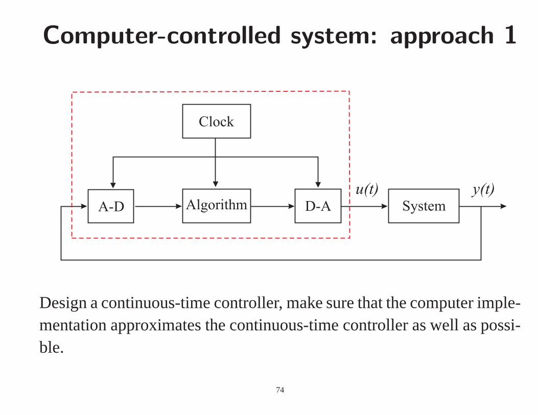
Computer-controlled system: approach 1

y(t)u(t)Algorithm

Clock

A-D D-A System

Design a continuous-time controller, make sure that the computer imple-mentation approximates the continuous-time controller aswell as possi-ble.

74

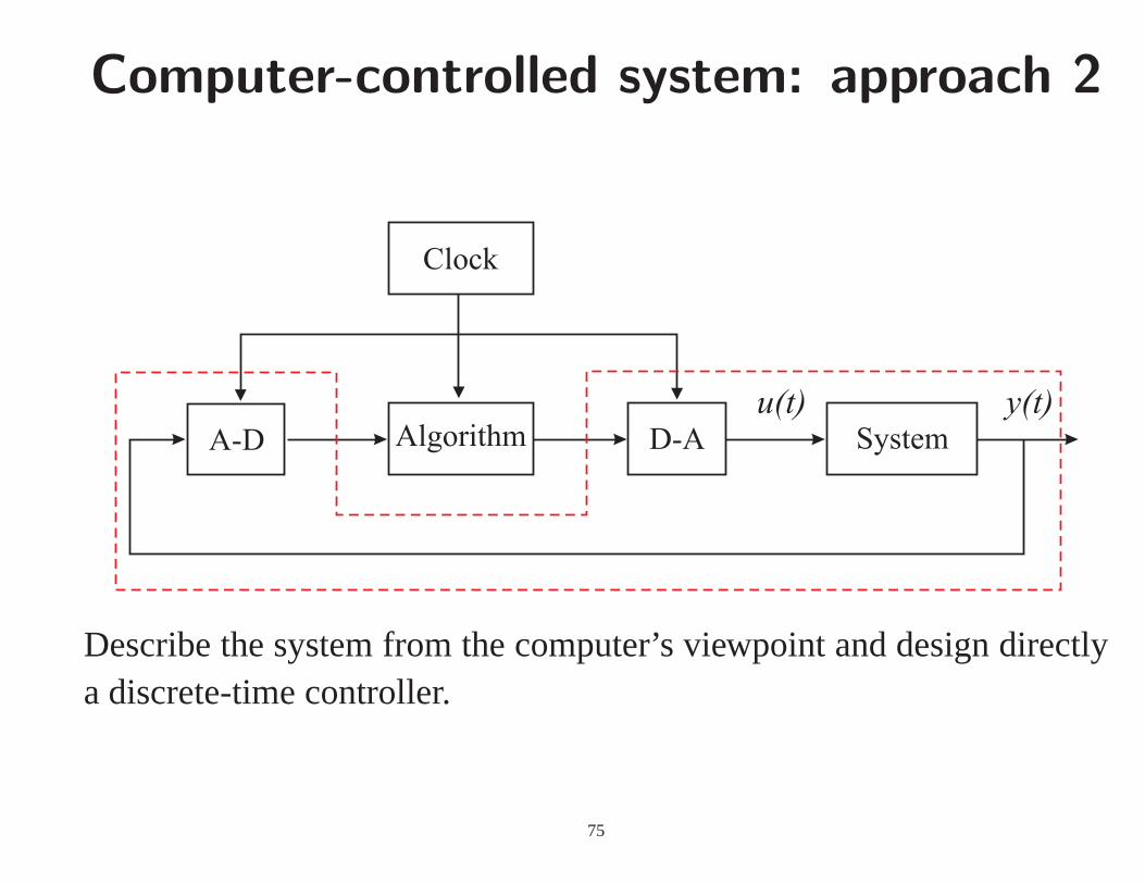
Computer-controlled system: approach 2

y(t)u(t)Algorithm

Clock

A-D D-A System

Describe the system from the computer’s viewpoint and design directlya discrete-time controller.

75

System from the computer’s viewpoint

y t( )u t( )System

Clock

{ ( )}y t k{ ( )}u tkA-DD-A

Describe system (including converters) at sampling instants only.

76

Zero-order hold

Timet t t t t t0 1 2 3 4 5

u(t) = u(tk), tk ≤ t < tk+1

Usuallytk+1− tk = const= h

77

Zero-order hold sampling of systems

Continuous-time system:

dx(t)dt

= Ax(t)+Bu(t)

y(t) = Cx(t)+Du(t)

Discrete-time system:

x(k+1) = Φx(k)+Γu(k)

y(k) = Cx(k)+Du(k)

with:

Φ = eAh , Γ =Z h

0eAsdsB, h. . . sampling period

78

MATLAB commands

G = ss(A,B,C,D); % LTI continuous-time state-space model

h = 0.1; % sampling period [s]

H = c2d(G,h); % convert to discrete time (ZOH)

G = d2c(H); % convert to continuous time (ZOH)

79

Selection of sampling period

Number of samples per rise time:Nr = Trh ≈ 4−10

0 5

−1

0

1(a)

0 50

1

0 5

−1

0

1(b)

0 50

1

0 5

−1

0

1(c)

0 50

1

0 5

−1

0

1(d)

Time

0 50

1

Time

a)Nr = 1

b) Nr = 2

c) Nr = 4

d) Nr = 8

80

Second order system

Nr = Trh ≈ 4−10 corresponds toω0h≈ 0.2−0.6

0 50

1

(a)

0 50

1

(b)

0 50

1

(c)

Time

0 50

1

(d)

Time

a) h = 0.125(ω0h = 0.23), b) h = 0.250(ω0h = 0.46),

c) h = 0.500(ω0h = 0.92), d) h = 1.000(ω0h = 1.83)

81

State feedback: basic problem formulation

• Model: x(k+1) = Φx(k)+Γu(k)

• Linear controller:

u(k) = −Lx(k)

• Design parameters: closed-loop poles, sampling interval

• Evaluation: comparex(k) andu(k) with specifications

(trade-off between control magnitude and speed of response)

82

Ackermann’s formula

ComputeL such that (Φ−ΓL) has a desired characteristic polynomial

P(z)

L = (0 . . . 0 1)W−1c P(Φ)

whereP(Φ) is the desired characteristic polynomial inΦ

in Matlab:

L = acker(Phi,Gamma,Po) (SISO, numeric problems)

L = place(Phi,Gamma,Po) (MISO, more robust)

83

Choice of desired poles

Using the continuous-time counterpart (2nd order)

s2+2ζωs+ω2

givesz2+ p1z+ p2 with

p1 = −2e−ζωhcos(

ωh√

1−ζ2)

p2 = e−2ζωh

in Matlab usec2d !

84

Linear quadratic control

J =N

∑k=1

xT(k)Qx(k)+uT(k)Ru(k)

Q, R are design parameters (weights)

A state feedback matrixL that gives a minimalJ can be found by solving

the Riccati equation.

Similar to pole placement, but no need to define poles!

In Matlab:dlqr(Phi,Gamma,Q,R) % state weighting

In Matlab:dlqry(Phi,Gamma,C,D,Q,R) % output weighting

85

State estimation: observers

x(k+1) = Φx(k)+Γu(k)

y(k) = Cx(k)

Input and output available, reconstruct the state:

• Direct calculation (requires differentiation)

• Luenberger observer (model-based)

• Kalman filter (optimal in presence of noise)

the terms “observer”, “estimator”, “filter” are in this context used syn-

onymously

86

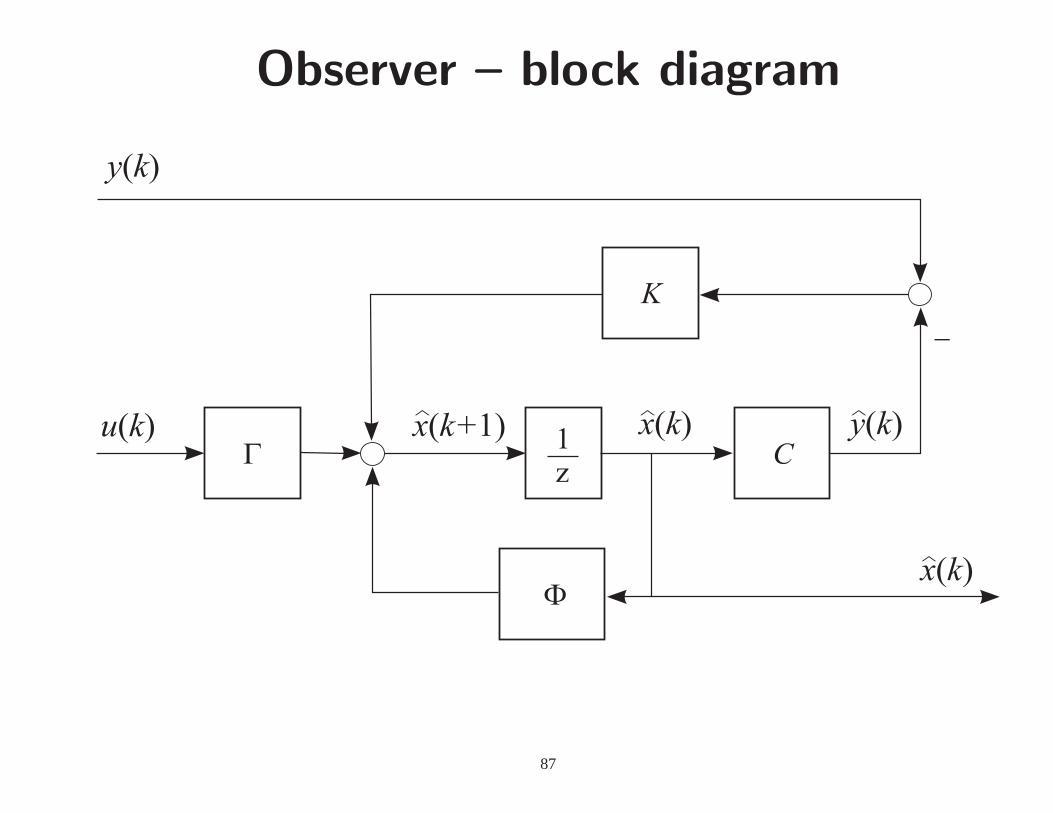
Observer – block diagram

K

1z

u k( ) x k+( 1)^ y k( )^

y k( )

Cx k( )^

x k( )^

-

87

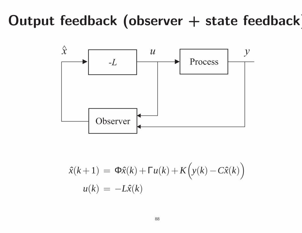
Output feedback (observer + state feedback)

x̂(k+1) = Φx̂(k)+Γu(k)+K(

y(k)−Cx̂(k))

u(k) = −Lx̂(k)

88

Poles of the closed-loop system

x(k+1) = Φx(k)+Γu(k)

e(k+1) = (Φ−KC)e(k)

u(k) = −L(x(k)−e(k))

x(k+1)

e(k+1)

=

Φ−ΓL ΓL

0 Φ−KC

x(k)

e(k)

Process poles:Ar(z) = det(zI−Φ+ΓL)

Observer poles:Ao(z) = det(zI−Φ+KC)

Separation principle

89

Servo case (two-degree-of-freedom)

Goal: respond to a reference signal in a specified way.Replaceu(k) = −Lx̂(k) by: u(k) = −Lx̂(k)+Lcuc(k)

ux^

Lc

Observer

Process-L

uc

y

90

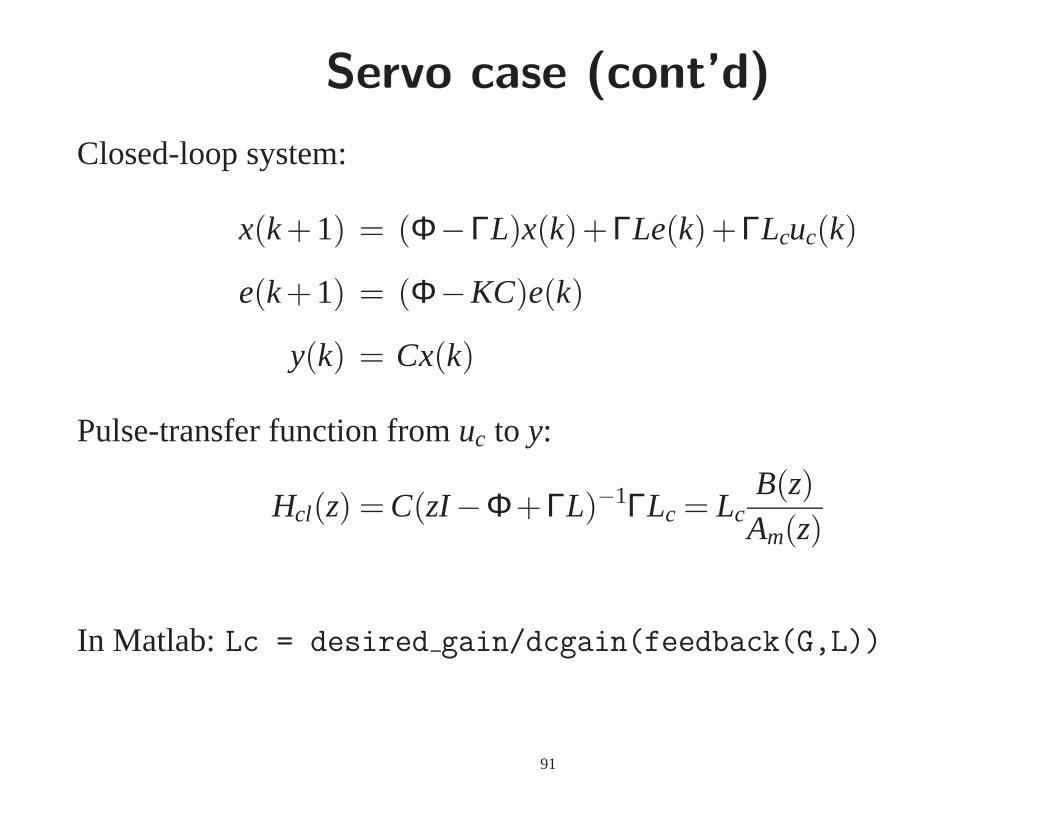
Servo case (cont’d)

Closed-loop system:

x(k+1) = (Φ−ΓL)x(k)+ΓLe(k)+ΓLcuc(k)

e(k+1) = (Φ−KC)e(k)

y(k) = Cx(k)

Pulse-transfer function fromuc to y:

Hcl(z) = C(zI−Φ+ΓL)−1ΓLc = LcB(z)Am(z)

In Matlab:Lc = desired gain/dcgain(feedback(G,L))

91

Application to a nonlinear system

Feedbackcontroller

ReferenceNonlinear

system

-

+

+

y0

y-

u0

+

+

+

y0

Feedforwardcontroller

Linear controllers must use signalsu, y, x !

92

PID control

The ”textbook” version

u(t) = K

(

e(t)+1Ti

Z t

e(s)ds+Tdde(t)

dt

)

More realistic PID controller:

U(s) = K

(

bUc(s)−Y(s)+1

sTi(Uc(s)−Y(s))−

sTd

1+sTd/NY(s)

)

93

Discrete-time PID

P-term:P(k) = K(buc(k)−y(k))

I-term: I(k+1) = I(k)+ KTi

e(k)

D-term: D(k) = TdTd+NhD(k−1)− KTdN

Td+Nh(y(k)−y(k−1))

u(k) = P(k)+ I(k)+D(k)

94

PID tuning

• Pole placement

• Root locus

• Bode diagram

• Tuning rules (Ziegler-Nichols,λ−tuning)

G(s) = e−t0s Kp

(τs+1)⇒ Kc =

τKp(λ+ t0)

, Ti = τ, Td =t02

95

Cascade control (example: inverted pendulum)

Reference Position controller Inverted

pendulumAngle

controller

96

Model-based adaptive control

u

Adaptation

Design parameters

Controller

-

Process

Linearmodel

yr

ym

97