Contents

List of Figures xvii

Preface xxxiv

Acknowledgments xxxvii

About the Author xxxviii

Part I Risk

1 What Is Risk? 3Price volatility 4

1. Price volatility: a first look – Methods 1 and 2 52. Ramping up sophistication – Method 3 73. A histogram of volatility distribution – Method 4 9

What is risk? 101. How should one think about risk? 122. Thinking about risk – from exposure to impact 12

Estimating exposure and impact – Emirates airline 141. What is Emirates’ exposure? 152. What is the trend for Emirates’ exposure? 153. What is the impact? 164. What is Emirates’ risk appetite? 185. Conclusions from the Emirates example 19

Parting words 21Annexure 1 – Building a histogram in EXCEL 22Annexure 2 – Trailing (rolling) correlations and volatilities 26

1. Rolling volatilities 262. Rolling correlations 31

2 Measuring Risk 34Exploring target accounts 34

1. Target accounts and management action: value at risk and stop loss limits 37

Introducing value at risk 381. What is value at risk? 392. Value at risk methods 403. Caveats, qualifications, limitations and issues 434. Risk or factor sensitivities 45

vii

PROOF

Calculating value at risk – step by step walkthrough 461. Methodology 462. VaR approach specific steps 513. Proof of equivalence: short-cut method versus

VCV matrix approaches to portfolio VaR 56Value at risk for bonds 65

1. Calculating VaR for bonds 65Annexure 1 – Calculating value at risk: a study of VaR flavors 73

1. Variance/Covariance (VCV) approach 752. Historical simulation approach 783. Monte Carlo simulation approach 804. Incremental VaR 825. Marginal VaR 846. Conditional VaR 867. Probability of shortfall 88

Annexure 2 – Value at risk application: margin lending case study 891. Designing a solution 90

Annexure 3 – Probability of default modeling using Merton’s structured approach 971. The valuation of firm equity as a call option on firms assets 98

3 Managing Risks 100A framework for risk management 100

1. Risk policy 1012. Good data and a first look at models 1033. Models and tools 1054. Metrics and sensitivities 1065. Limits and control process 1116. Conclusion 115

Setting limits 1151. Capital loss and stop loss limits 1152. Value at risk limits 1203. Regulatory approach limits 1224. Other market risk limits 1235. Credit risk limits 1246. Application to products 1297. Setting limits for liquidity risk 1308. Setting limits for interest rate risk 1319. Limit breach, exception processing,

action plan for trigger zones 131Annexure 1 – Setting stop loss limits 133

1. A guide to setting stop loss limits 133

viii Contents

PROOF

2. Stop loss limits example and case study 1333. Setting stop loss limits – limit review triggers and

back testing 138Annexure 2 – Risk metrics 141

1. Holding period return 141 2. Standard deviation/volatility (Vol)/s 141 3. Annualized return 141 4. Annualized volatility 142 5. Duration 142 6. Convexity 142 7. Sharpe ratio 143 8. Put premium 144 9. Beta with respect to market indices 14410. Treynor ratio 14511. Jensen’s Alpha 14512. Correlation coefficient, r 14613. Portfolio volatility taking into account correlations 14914. Volatility trend analysis 150

4 Building Risk Systems 151Treasury and market risk 153

1. The challenge with treasury risk management 154The credit risk function 156

1. What does credit management involve? 157The survival of risk 162Assessment framework 162

1. The risk survival information flow design 1642. Risk systems for central banks 165

5 Stress Testing, Bank Regulation and Risk 168Stress testing 168

1. A stress testing framework 169Evolution of banking regulation 174

1. The great depression and Regulation Q 1742. Basel I and amendments to the capital accord 1753. Basel II 1764. Basel III 1815. Comprehensive capital analysis and review

(CCAR) – the US response 185Why doesn’t bank regulation work? 187Annexure 1 – Capital estimation for liquidity risk management 189

1. Liquidity reserves: real or a mirage 1902. Estimating capital for liquidity risk: the framework 194

Contents ix

PROOF

x Contents

Annexure 2 – Liquidity driven bank failures and near misses 1951. Case study: Bear Stearns 1952. Case study: Lehman Brothers 1993. Case study: American International Group (AIG) 204

Part II Monte Carlo Simulation

6 Monte Carlo Simulators in EXCEL 213Building Monte Carlo Simulators in EXCEL 213

1. Introduction 2132. What is a Monte Carlo simulator? 2153. The process or generator function 2154. Building your first MC simulator model 2165. Extending MC simulation models to

currencies and commodities 2206. MC simulations models – understanding drift,

diffusion and volatility drag 2207. Linking Monte Carlo simulation with binomial

trees and the Black Scholes model 2268. Simulating interest rates using CIR (Cox Ingersoll

Ross) and HJM (Heath, Jarrow & Merton) 2289. Monte Carlo simulation using historical returns 229

10. Option pricing using Monte Carlo simulation 23611. Convergence and variance reduction techniques for

option pricing models 254

7 Simulation Applications 2621. Monte Carlo simulation VaR using historical returns 262

1. Monte Carlo simulation – early days 2622. Monte Carlo simulation revisited – fixing the distribution 2633. Monte Carlo simulation and historical returns –

calculating VaR 2642. Monte Carlo simulation: fuel hedging problem 273

1. Case context and background 2732. Simulating crude oil prices 2773. Linking financial model to the simulation 2824. Tweaking the model and making it more real 2875. Jet fuel price shock estimation 2896. Shortfall using Monte Carlo implementation 2907. Presenting the case to the client 294

3. Simulating the interest rate term structure 3001. CIR interest rate model 300

PROOF

Contents xi

4. Forecasting the monetary policy rate decision for Pakistan 3031. Process 3032. Results 305

Part III Fixed Income and Commodity Markets – Dissecting Pricing Models

8 Identifying Drivers for Projecting Crude Oil Prices 313The 2009 crude oil price outlook 313

Data 314The debate 314

Conclusion – the 2009 debate 319Revisiting the model – 2013 320

Revised data 320References 326

9 Gold and the Australian Dollar 327Gold prices – drivers, trends and future prospects 327Gold price and Australian dollar – relationship reviewed 329

10 Relative Value and the Gold–Silver Ratio 335Relative values 338Gold’s value – Gold to silver ratio 344Weakness of reserve and safe haven currencies 345Gold–silver ratio as trading signal? 347

11 Correlations: Crude Oil and Other Commodities 350West Texas crude oil 352Fuel oil 354Diesel fuel 355Natural gas 357Gold 358Silver 360Platinum 361Aluminum 363Steel 364Copper 366Cotton 367Corn 369Wheat No. 2 370Wheat No. 1 372Coffee 373Sugar 375

PROOF

xii Contents

Corn oil 376Soybean oil 378Crude palm oil 379

12 Crude Palm Oil Futures 381Data 381Price levels 382Annualized volatility and 10-day holding VaR 383Volatility trends 383Correlations and scatter plots 384

USD–EUR 384MYR–USD 385Gold 386West Texas Intermediate (WTI) 387Wheat No. 2 388Corn 389

13 Crude Oil and Inflation 391Components of price indices 391Consumer price index 394Wholesale price index 400

14 Historical Spreads in Bond Yields in the Indo-Pak Sub-Continent 404Data 404Note on inflation rates 405

Bond yields and inflation in Pakistan – a first look at real rates 407

Bond yields and inflation in India – a first look at real rates 411A comparative analysis: India and Pakistan 416

15 Volatility Trends in Commodity Prices 424Commodities 424

Annualized volatility 424Trend 4253-Sigma band 428Commodity correlations 429

16 Energy Insights 438Overview – US 438

1. Natural gas 4382. Crude oil 4423. Relationship between crude oil and natural gas prices 446

Overview – China 4481. Oil 4492. Natural gas 450

PROOF

Contents xiii

3. Coal 452Overview – India 453

1. Crude oil 4532. Natural gas 455

Overview – Pakistan 456

Part IV Derivative Securities

17 Derivatives Terminology 463Forward contracts 464

The investment bank intern 464Futures contracts 465Options 466

Maturities and exercise date 466Payoff profiles 467

The payoff profile for a forward contract 468Payoff profiles for calls and puts 470Building blocks and synthetic configurations 473

18 Products and Pricing 4761. Standard template for evaluating derivatives 4772. Options 479

Option price 4813. Forward contracts 486

Forward price 4874. Futures contracts 488

Futures price 4895. Swaps 489

Interest rate swap (IRS) 489Currency swap 490

19 Variations 4911. Options 491

Stock options 491Foreign currency options 491Index options 491Futures options 492Warrants 492Employee stock options 492Convertibles 493Interest rate options 493Bond options 493Interest rate caps/floors/collars 493European swap options 495

PROOF

Exotic options 495Bermuda option 495Quanto option 496Composite option 496Digital or binary or “all or nothing” options 496Barrier options 496Asian options 497Average strike options 497Look back options 497Compound options 498Chooser (as you like it) options 499Exchange options 499Forward start options 499Basket options 499Shout options 500

2. Forwards 500Synthetic forward contract 500Forward rate agreement (FRA) 500

3. Futures 501Stock index futures 501Futures contracts on currencies 501Futures contracts on commodities 501Interest rate futures 501

4. Swaps 502Fixed for fixed currency swap 502Floating for floating currency swap 503Cross-currency interest rate swap 503Step-up swaps 503Amortizing swaps 503Basis rate swap 503Forward or deferred swaps 503Compounding swaps 503LIBOR-in-arrears swap 503Constant maturity swap 504Constant maturity treasury swap 504Differential swap or quanto 505Variance or volatility swap 505Equity swap 505Commodity swap 506Asset swap 506Accrual swap 506Cancellable swap 506

xiv Contents

PROOF

Contents xv

Extendable swap 506

20 Derivative Pricing 507Relative pricing and risk neutral probabilities 507Binomial option pricing 507Spreadsheet implementation of two-dimensional binomial tree 510

European call option 511European put option 513American call option 513American put option 514

Pricing European call options using Monte Carlo simulation 515Pricing exotic options using Monte Carlo simulation 520

Vanilla call, put options and exotic Asian and look back cousins 521Pricing barrier and chooser options 523Pricing ladder options 525

21 Advanced Fixed Income Securities 529Cash flows 529Discounting cash flows 529

Spot rates 530Forward rates 530Short rates 531Yield to maturity 531

Term structure of interest rates 532Forward rate agreements (FRA) 533Forward contracts 533Swaps 534

Pricing interest rate swaps 534Pricing cross currency swaps 546Caps and floors 553Accrual swaps 555Value of regular swap 557Range accrual note 558Commodity linked note 560

Annexure 1 – How to determine spot rates and forward rates and yield to maturity 562How to determine forward rates from spot rates 562How to determine spot rates from forward rates 563How to calculate the YTM of a bond 565Trial and error process for calculating YTM of a bond 565EXCEL’s goal seek method for calculating YTM of a bond 567

PROOF

xvi Contents

22 The Treasury Function 569Trade flows (FX desk) 569The Treasury function operations 570

Front office function 570Middle office function 572Back office function 572

Related terminologies 574Four eyes 574Confirmation 575Society for Worldwide Interbank Financial

Telecommunications (SWIFT) 575Settlement 576Price discovery 576Proprietary trading 576Operational risk 577

23 Advanced Products 578Structured products 578

Cross currency swaps 578Participating forwards 578Equity linked notes 579Capital protected/capital guaranteed notes 581Commodity linked notes 582Range accruals 583Switchable 584Interest rate differential (IRD) trades 585

Credit products 590Credit default swaps 590Total return swaps 593Collateralized debt obligation (CDO) 594

Notes 595

Bibliography 598

Index 603

PROOF

Part I

Risk

Working with volatility

Measuring risk

Target accounts

Building risk systems

Why doesn’t bank regulation work?

PROOF

PROOF

1What Is Risk?

Risk is uncertainty. Risk is opportunity. Risk is misunderstood.An uncertain outcome requires planning to manage the downside. Risk management is the field that specializes in managing the downside of uncertain outcomes.

Just like any other business process, risk management requires a com-bination of intuition and common sense, mixed with the right processes and controls. Intuition and common sense come with experience, while processes and controls are organizational design problems. How the above four elements are balanced determines the effectiveness of risk manage-ment. With the right mix the recipe works; take one element out of align-ment and it stops functioning.

Is risk limited to just the financial services industry? Or are there broader applications that cross over beyond boundaries of markets and prices? If you are not a large bank or a hedge fund manager, do you still need to think about risk?

The truth is that we are tuned to think about risk at an intuitive level. We just have to look around ourselves to see that thinking at work.

Think about an important desired outcome such as attending a busi-ness meeting on time. To ensure you are not late (negative outcome), you will look up directions (preparation) and leave a little early (prevention) so that you can reach the appointment on time (desired outcome) or a little early (preferred outcome).

A few more examples on how we think about risk are given below:

If you are stuck in traffic (uncertainty), you will look at alternate routes (a) (management) or call ahead (hedging) to let your client know (manag-ing expectations). The next time you head in the same direction you will adjust your behavior (learning and adaptability) based on how long it took you to finally get to your destination. If you make the same trip on a daily basis, your behavioral adjustments will fine-tune

3

PROOF

4 Models at Work

themselves using average, likely and unlikely conditions (data set and probabilities). If there are powerful incentives (large business deal or a promotion) or penalties the game will change again depending on how you read and interpret them.What if you are a manufacturer, trader and supplier of goods? Apply (b) the same principles to lock in costs before input prices rise to ensure that your margins are protected and remain within an acceptable range (desired outcome). If you run the sales function, how do you ensure revenues and profitability meet the year-end quota even if the average unit sale price falls?Think like a project manager for a large construction site. How do you (c) ensure that you deliver on time and under budget (desired outcome)? What are the biggest challenges to these two desired outcomes? How do you track them? What are the possible causes of uncertainty that can derail your plans? How do you address them?

These are all applications of risk management. Some occur at an intuitive level, others involve tools and frameworks. The science is just an exten-sion of the same.

Price volatility

Let’s begin with a simple example: prices.As traders1, manufacturers of goods, construction site project managers

or the heads of proprietary desks for banks, we all care about the move-ment of prices as well as their timing.

Price risk is not the only risk we are exposed to. It is, however, one that is easily quantifiable, using objective data (historical prices) and statistical models and tools (volatility and distribution). For that one reason it pro-vides a great canvass for showcasing our risk management framework.

What do we know about price movement? Prices go up and down, as well as sideways. Once upon a time they used to move within reasonable ranges; occasionally you could factor in seasonality, and predict the direc-tion and size of the movement. The modeled price ranges were factored in when you drew your budget.

Today prices move abruptly and without notice, ignoring budgets, quo-tas, reasonable historical behavior, profitability or economic impact. You can model supply and demand as well as market sentiment, but your model price will fail to track the actual market price on days that count.

Do price changes impact all of us the same way? If you trade on a daily basis and bring your investments down to zero when markets close, you care about price changes that occur during trading hours (intraday price movements). However, if you buy steel and concrete mix every week and

PROOF

What Is Risk? 5

are planning on buying it for the next two hundred weeks, do intraday price changes matter? They don’t.

Unfortunately, if you are a non-trader married to price volatility as a buyer, seller or inventory holder, when it comes to managing price risk your reaction time is simply not fast enough.

Price changes are measured through volatility, an alternate term for standard deviation. Volatility tracks historical price movements and does a reasonable job of indicating the range of prices we are likely to see over a given period. Every now and then it misbehaves and breaks down. But for most applications standard deviation is a good first indicator of risk and price behavior.

In the field of risk management volatility is the beginning and the end. It has many names, some more fashionable than others, but the most com-mon you are likely to see is volatility or vol. (a common trade short form). As with the many names, there are just as many variations when it comes to calculating volatility . The reason why volatility is important is because it is one of the four elements that define the distribution of returns. The other three are the location or center defined by the mean ; skewness , a measure of symmetry that could be positive or negative, indicating which direction the distribution leans toward; and kurtosis, which on a relative basis represents how tall the distribution is and how fat its tails are.

Take one statistical measure, sprinkle a few crude assumptions, apply some presentation lessons and you can take a rough shot at estimating risk. Sophistication in models gets added across all three dimensions – measurement, assumptions and presentation. More sophisticated models have a higher breakage frequency since a better fit (read: more param-eters, higher accuracy) for one data set is no assurance for the future fit on untested data sets. Adjustments and tweaks only add value when they improve explanatory power2.

1. Price volatility: a first look – Methods 1 and 2

Are markets today more volatile? It certainly feels that way. This is possi-bly because of the speed with which markets now move and the reaction time of traders to news. Do we have any objective evidence that supports this assertion? Let’s try out a few approaches that give us an indication of how volatility has moved across time and markets.

Figure 1 shows one way of viewing price volatility for three commodi-ties, gold, crude oil and cotton, by using a plot of daily price changes (daily returns)3.

A daily returns plot tracks the percentage change in prices on a daily basis. The changes are first order changes, since we are only looking at relative price change from one period to the next. The plot can be used to

PROOF

6 Models at Work

eyeball the average price change (the benchmark) as well as time intervals where prices became more volatile. For instance:

For oil we can see that there was a period of volatile price changes (a) between mid 2008 and mid 2009, see-sawing as much as +15 percent in one day and −12 percent on others.For cotton, price volatility died down in the period immediately fol-(b) lowing the fall in crude oil volatility in mid 2009 (the result of the global recession and its impact on textiles manufacturers’ demand for cotton).While gold has generated significant returns during this time frame, (c) on a relative basis its price volatility has been the lowest when com-pared with the volatilities of the other two commodities.

Eyeballing the chart above serves us well for basic insight. It gives us an initial sense of the range within which price changes are likely to move for the three commodities.

We can take the same daily returns data set and draw a histogram using EXCEL spreadsheet tools to get a better sense of the distribution of price changes.

Change in the value of gold (US dollar amount) – oilinsights.net

Gold-USD

8.00%

4.00%

0.00%

12.00%

–8.00%

–12.00%

–4.00%Dai

ly r

etur

ns

15.00%10.00%

5.00%

20.00%

–5.00%–10.00%

–15.00%

0.00%

Dai

ly r

etur

ns

20.00%15.00%10.00%

25.00%

–5.00%–10.00%–15.00%–20.00%–25.00%

5.00%0.00%

Dai

ly r

etur

ns

–– WTI-USD

–– Cotton-USD

Change in the value of WTI (US dollar amount) – oilinsights.net

Change in the value of cotton (US dollar amount) – oilinsights.net

8-Mar-10 28-Nov-10 20-Aug-11

3-May-06 30-Aug-07 26-Dec-08 24-Apr-10 21-Aug-11

5-Jan-05 4-May-06 31-Aug-07 27-Dec-08 25-Apr-10 22-Aug-11

3-Jan-08

4-Jan-05

24-Sep-08 16-Jun-09

Figure 1 Daily return plot for gold, oil and cotton – January 2008 to August 2011

PROOF

What Is Risk? 7

For instance, Figure 2 uses a daily return series calculated for fuel oil prices from 2008 to 2011. But rather than plotting daily price changes we bucket price changes together and do a count of how many price changes fall in a given bucket. Once the results are tabulated we plot them in a chart. The chart output and the tabulation are shown side by side.

We have just built our first histogram of the distribution of fuel oil price changes.

A histogram uses the same data (relative price changes) but provides a different visual perspective (distribution of price changes).

The distribution plot provides a clear summarized view of the entire dataset. We can see that the most common percentage change lies between −1 percent and +1 percent. The average change is no change (0 percent). The two extreme price changes in a given day are a fall of 18 percent and a rise of 11 percent.

We have moved further with our attempts at understanding price vola-tility. Our initial plot was a simple dump of daily price movement; useful but limited in insights that could be gained from looking at it.

2. Ramping up sophistication – Method 3

Our next image presents a more sophisticated view of price volatility. Volatility, like prices, is not constant. Imagine the implications of this on models that work with the assumption of constant volatility.

0.00%

20.00%

40.00%

60.00%

80.00%

100.00%

120.00%

0

–18%

–16%

–14%

–12%

–10% –8

%–6

%–4

%–2

% 0% 2% 4% 6% 8% 10%

Mor

e

50

100

150

200

250

Frequency Cumulative %

Figure 2 Daily return histogram for fuel oil – 2008 to 2011

PROOF

8 Models at Work

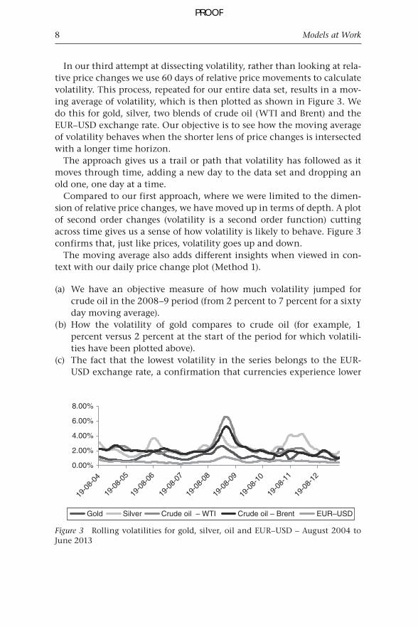
In our third attempt at dissecting volatility, rather than looking at rela-tive price changes we use 60 days of relative price movements to calculate volatility. This process, repeated for our entire data set, results in a mov-ing average of volatility, which is then plotted as shown in Figure 3. We do this for gold, silver, two blends of crude oil (WTI and Brent) and the EUR–USD exchange rate. Our objective is to see how the moving average of volatility behaves when the shorter lens of price changes is intersected with a longer time horizon.

The approach gives us a trail or path that volatility has followed as it moves through time, adding a new day to the data set and dropping an old one, one day at a time.

Compared to our first approach, where we were limited to the dimen-sion of relative price changes, we have moved up in terms of depth. A plot of second order changes (volatility is a second order function) cutting across time gives us a sense of how volatility is likely to behave. Figure 3 confirms that, just like prices, volatility goes up and down.

The moving average also adds different insights when viewed in con-text with our daily price change plot (Method 1).

We have an objective measure of how much volatility jumped for (a) crude oil in the 2008–9 period (from 2 percent to 7 percent for a sixty day moving average).How the volatility of gold compares to crude oil (for example, 1 (b) percent versus 2 percent at the start of the period for which volatili-ties have been plotted above).The fact that the lowest volatility in the series belongs to the EUR-(c) USD exchange rate, a confirmation that currencies experience lower

0.00%

2.00%

4.00%

6.00%

8.00%

19-0

8-04

19-0

8-05

19-0

8-06

19-0

8-07

19-0

8-08

19-0

8-09

19-0

8-10

19-0

8-11

19-0

8-12

Gold Silver Crude oil – WTI Crude oil – Brent EUR–USD

Figure 3 Rolling volatilities for gold, silver, oil and EUR–USD – August 2004 to June 2013

PROOF

What Is Risk? 9

volatility than commodities. In turn, commodities are, in principle, exposed to higher volatility compared to equities, with the exception of gold.

3. A histogram of volatility distribution – Method 4

Our last variation on dissecting volatility brings the best of these two worlds together – calculating rolling volatilities to get a moving average and then graphing a distribution plot or histogram on them, as shown in Figure 4.

Why do we need this?We already know that volatility is not constant; we know that it goes

up and down from the preceding example. If you are building a price model that uses underlying volatility, which value should you pick? The most likely candidates lie within the 1.7 percent – 2.4 percent range. You can pick the number closest to the average and use 2 percent. Or you can stress your model and see what a spell of high volatility could do to prices and use 5 percent. In either instance it would be useful to know what the actual likelihood of either of these two events (a realized volatility of 2 percent vs. a realized volatility of 5 percent) is.

The volatility distribution given above already provides us with the actual likelihoods for the given volatility buckets plotted. With it we can easily map out the distribution. For fuel oil the most common volatility is 2 percent (with an actual likelihood in the given data set of almost 13 percent, that is, 13 days in every 100 days), and the midpoint of the distribution is 2.2 percent. The two extremes are a low of 1.1 percent and a high of 5.8 percent and upwards (with actual likelihoods in the given data set of 0.1 percent and 0.5 percent respectively).

0.00%20.00%40.00%60.00%80.00%100.00%120.00%

0

1.1%

1.4%

1.7%

2.0%

2.4%

2.7%

3.0%

3.4%

3.7%

4.0%

4.4%

4.7%

5.0%

5.3%

5.7%

Mor

e

50

100

150

Frequency Cumulative %

Figure 4 Distribution of fuel oil volatility – 2008 to 2011

PROOF

10 Models at Work

What is risk?

Now compare all of the above iterations of evaluating price volatility to the simplest of tools used by ordinary mortals: a plot of absolute price levels depicting daily highs and lows – the one-dimensional price chart shown in Figure 5.

Which of the five approaches shared so far would you prefer?

The absolute price chart1. The relative price return plot2. The distribution/histogram of price changes3. The rolling volatility plot4. The distribution/histogram of volatility.5.

When I put this question in front of my students, a common pushback is with my earlier statement about model sophistication – Occam’s razor. Do we really need this sophistication? Isn’t a simpler model better? What is needed is sophistication in analysis, not complexity in models. These are two very different worlds. The volatility dissection process that we have followed is just one way of getting a better grip on the expected future behavior of prices.

Irrespective of the approach picked, you should notice one common trend. Risk, volatility and price movements are not constant. They range. They have seasons. They go through violent mood swings. Some years are better than others. Some years are disasters.

Each method has a place in the tool kit of a risk analyst. Rather than look-ing at a single dimension (absolute prices) we look at multiple dimensions. We plot relative price changes, we review distribution histograms, we track rolling volatility and we dissect the distribution of rolling volatility.

160

140

120

100

Per

bar

rel o

f WT

I

3-Jan-05 2-May-06 29-Aug-07 25-Dec-08 23-Apr-10 20-Aug-11

80

60

40

20

WTI prices in USD

Figure 5 Daily price series of crude oil

PROOF

What Is Risk? 11

The key word here is distribution. Price or volatility, an understanding of the distribution is an understanding of the risk involved. If you want to be comfortable with understanding risk, you must understand the dis-tribution of risk.

As can be seen in Figure 6, if you traded in risk, 2008, 2009 and 2011 were great years based on their high volatility index. By contrast, 2012 was a terrible year for risk traders given the lowest levels of volatility in the eight year period plotted. There was uncertainty, but nothing like the lev-els of 2008. Traders like risk and uncertainty because uncertainty breeds opportunity and trades. Stability is great for grandmothers and Warren Buffett but toxic as cyanide for trading Profit & Loss (P&L) accounts.

As ordinary mortals, not traders, we tend to misread risk. We do a poor job of forecasting, estimating and assessing risk because we don’t deal with it on a daily basis. We assume that our intelligence, our background and our experiences give us license to forecast the direction and magni-tude of the next wave of risk, but we are often wrong. We overcompen-sate. We are cautious. We ignore history and trends in favor of our own biases. We play it safe.

A safe player, not raised on a strict diet of trading and risk, would never forecast a three-times jump in underlying volatility in the Euro-USD exchange rate. In fact, with the stability and strength in Euro seen in 2008 and early 2009, we would have been laughed out of most board-rooms for suggesting such an event. The prevalent school of thought in

Gold vol index

Siver vol index

Oil (WTI) vol index

Oil (Brent) vol index

EUR–USD vol index 1.00

3.24

3.29

3.78

1.48

2004–

2.00

4.00

6.00

8.00

10.00

12.00

Axi

s tit

le

2005 2006 2007 2008 2009 2010 2011 2012 2013

1.06

1.92

1.36

1.23

0.481.15

3.72

3.86

5.36

2.774.12

8.97

5.26

4.26

1.671.55

5.04

5.08

5.36

2.703.88

6.51

10.37

8.74

1.971.55

5.95

6.94

7.29

4.352.35

4.06

4.44

4.34

0.801.14

5.10

4.69

6.72

4.051.76

3.90

5.84

5.56

1.38

Figure 6 Risk assessment: volatility index, ten years – 2004 to 2013 Source: FinanceTrainingCourse.com

PROOF

12 Models at Work

early 2008 predicted the demise of the US dollar as a global reserve cur-rency and its replacement by the European Union Standard, even more so after the 2008 asset backed security crisis in US markets.

Yet the Euro fell from its April 2008 exchange rate high of 1.595 USD to a low of 1.19 USD, and saw an even steeper intraday low with unheard of 2 percent negative moves in the first and second quarters of 2011 (see Figure 7).

1. How should one think about risk?

Risk is uncertainty. Risk is opportunity. Risk is misunderstood.Here is a simple rule. Don’t think in terms of absolutes and averages.

Think in terms of levels, trends and scales.The risk is not that you will get the average or the averaging period wrong.

The risk is that you will misread the level and threshold of risk you are facing. You will misread the change and miss the transition to the next level of intensity.

Expect the unexpected to misbehave and surprise you. It will.

2. Thinking about risk – from exposure to impact

Before your family physician prescribes any medicine or procedure he has to diagnose what is wrong: an upcoming season for the influenza virus – a flu shot; a muscular injury – an anti-inflammatory painkiller; an infection – antibiotics; a fracture – a splint.

The same holds true for risk. Before we decide on our approach for managing risk we have to understand what are we exposed to. With financial risk management this translates into determining a numerical

4.00%

3.00%

2.00%

1.00%

0.00%

–1.00%

–2.00%

5-Jan-04

5-May-04

5-May-05

5-Sep-04

5-Sep-05

5-Jan-05

5-May-06

5-Sep-06

5-Jan-06

5-May-07

5-Sep-07

5-Jan-07

5-May-08

5-Sep-08

5-Jan-08

5-May-09

5-Sep-09

5-Jan-09

5-May-10

5-Sep-10

5-Jan-10

5-May-11

5-Sep-11

5-Jan-11

5-May-12

5-Sep-12

5-Jan-12

–3.00%

EUR

Figure 7 Risk assessment: EUR–USD exchange rate, daily rate changes, eight years – 2004 to 2012

PROOF

What Is Risk? 13

value for your risk. We call this numerical value exposure. Exposure is a gross number that may indicate consumption, position, size or amount. While the actual risk is dependent on exposure, exposure is not risk.

If you drive a car, the chances of you making a claim on your insur-ance policy are directly linked to the number of miles you drive in a year and the neighborhoods you drive in. Within investments, portfolios and commodities, exposure is the analogous number to miles driven and the neighborhoods driven through. Its most common manifestation is the total investment value or the dollar sum of all of your positions. If you run a book of 200 million USD that 200 million USD is your exposure. Your risk will be measured in terms of that number.

The next step is to examine the trend of exposure to ensure that you adjust for seasonality and don’t over or under estimate exposure. Armed with these two elements you are now ready to calculate the actual risk or the financial impact of uncertainty. We do this by tracking exposure and matching it with the relevant risk drivers or factors. The combination of these two elements (exposure and risk factors) creates a number, which is uncertain and volatile. We label it impact. Impact, unlike exposure, is measured on a net basis and represents the amount at risk of the un-hedged exposure.

This leads us to four questions that we need to answer before we can complete our diagnoses of risk.

What is the exposure?1. What is the trend for the exposure?2. What is the impact of the risk factors on exposure?3. What is our risk appetite?4.

Let’s look at how these numbers can be estimated.Four examples follow. Four businesses exposed to either a rise in fuel

prices or changes in exchange rates or movements in input (commodities) prices. The industries in question are airlines, trading houses, exporters and goods manufacturers, respectively.

Exposure Trend Impact Capital

Figure 8 Risk management framework

PROOF

14 Models at Work

Estimating exposure and impact – Emirates airline

Emirates is a leading Middle Eastern airline known for its commitment to redefining business travel and operating the largest business and first class transit lounges in the world, at Dubai Airport. Emirates flies 40 million passengers a year and its last reported financial year (2012–13) grossed just under 20 billion USD in annual revenues. It employs 50,000 employ-ees spread across six continents and its fleet includes 200 aircraft.

As air travel has rebounded and jet fuel prices have climbed, Emirates has seen its profits erode despite rising revenues. Profit margins have plummeted from a high of 9.9 percent in 2010–11 to 3.1 percent in 2012–13. Margins have also impacted returns on shareholders’ funds, which dropped from a high of 28 percent in 2010–11 to 10 percent in 2012–134.

Yet Emirates decided to leave its jet fuel exposure unhedged for the last two years. Why is that? To answer this question we have to dig a little deeper. We have to find out the actual amount at risk and then compare it with Emirates’ internal outlook on fuel prices.

We will do that using the four questions we have just identified in the preceding section. Exposure. Trend. Impact. Risk Appetite.

BUSINESS EXPOSURE RISK FACTOR IMPACT

Airlines Jet fuel price

volatility. Demand

shifts on account of

recession

Fuel prices move

up. Limited ability to

raise ticket prices

Dollar impact on

fuel bill on account

of jet fuel price

changes

Importers of

Audi 4 door

sedans

Payment for imports

in Euro due in 90

days

Appreciation of

Euro against base

currency

Change in the

amount due in

base currency

on account of

appreciation of Euro

Exporters of

textile products to

Japan

Payment for exports

to be received in

120 days

Depreciation of

Yen against base

currency

Change in the

amount received

in base currency

on account of

depreciation of Yen

Auto part

manufacturers

Fixed price contract.

No room for

changes on account

of input cost

Rise in the price of

input components

Impact of change

in the price of the

basket of inputs on

profi tability

Figure 9 Examples of exposure, risk factor and impact

PROOF

What Is Risk? 15

1. What is Emirates’ exposure?

As Emirates grows its network and passenger handling capacity, its fuel bill is also rising. Emirates consumed 7.2, 6.1 and 5.1 million tons of jet fuel in the last three financial years respectively (most recent to past). In dollar terms, Emirates’ fuel bill was 7.5, 6.6 and 5.7 billion USD for the same time periods, shown in Figure 10.

Therefore, the most recent jet fuel exposure is 7.2 million tons. The same exposure in USD equivalent terms is 7.5 billion USD.

2. What is the trend for Emirates’ exposure?

Emirates’ fuel exposure is rising. While we assume that there is some seasonality in fuel consumption, we don’t have enough data available through public disclosure to estimate that.

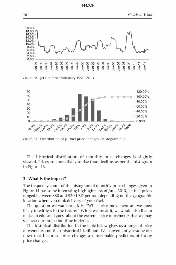
However, we do have price, rolling volatility and distribution data for jet fuel on a monthly basis, which is shared in Figures 11, 12 and 13 respectively.

We can see that while prices started rising in 2009, they have stayed at their high levels since 2010. Price volatility, on the other hand, has dropped to historical lows over the same period. Average monthly histori-cal volatility is about 9 percent. Recent monthly volatility has hovered around 5 percent.

00.5

11.5

22.5

33.5

44.5

May

-90

Mar

-91

Jan-

92N

ov-9

2S

ep-9

3Ju

l-94

May

-95

Mar

-96

Jan-

97N

ov-9

7S

ep-9

8Ju

l-99

May

-00

Mar

-01

Jan-

02N

ov-0

2S

ep-0

3Ju

l-04

May

-05

Mar

-06

Jan-

07N

ov-0

7S

ep-0

8Ju

l-09

May

-10

Mar

-11

Jan-

12N

ov-1

2

Figure 11 Jet fuel price series 1990–2013

Figure 10 Fuel expense and consumption for Emirates

PROOF

16 Models at Work

The historical distribution of monthly price changes is slightly skewed. Prices are more likely to rise than decline, as per the histogram in Figure 13.

3. What is the impact?

The frequency count of the histogram of monthly price changes given in Figure 14 has some interesting highlights. As of June 2013, jet fuel prices ranged between 880 and 920 USD per ton, depending on the geographic location where you took delivery of your fuel.

The question we want to ask is: “What price movement are we most likely to witness in the future?” While we are at it, we would also like to make an educated guess about the extreme price movements that we may see over our projection time horizon.

The historical distribution in the table below gives us a range of price movements and their historical likelihood. We conveniently assume (for now) that historical price changes are reasonable predictors of future price changes.

0.0%2.0%4.0%6.0%8.0%

10.0%12.0%14.0%16.0%18.0%20.0%

Jun-

91

Jun-

92

Jun-

93

Jun-

94

Jun-

95

Jun-

96

Jun-

97

Jun-

98

Jun-

99

Jun-

00

Jun-

01

Jun-

02

Jun-

03

Jun-

04

Jun-

05

Jun-

06

Jun-

07

Jun-

08

Jun-

09

Jun-

10

Jun-

11

Jun-

12

Figure 12 Jet fuel price volatility 1990–2013

0.00%

20.00%

40.00%

60.00%

80.00%

100.00%

120.00%

0

–32.

9%

–28.

2%

–23.

4%

–18.

7%

–14.

0%–9

.3%

–4.5

%0.

2% 4.9%

9.7%

14.4

%19

.1%23

.9%

28.6

%33

.3%

Mor

e

10203040506070

Figure 13 Distribution of jet fuel price changes – histogram plot

PROOF

What Is Risk? 17

Using the two tools (the histogram chart and the frequency table) we can see that the probability of a price rise is significantly higher than that of a price decline. Based on the cumulative probability table and plot the probability of a price decline is 22 percent. The probability of a price rise is 77 percent.

On the extreme movement front there is a 3.6 percent chance of see-ing a price rise of greater than 9.7 percent in any given month. The odds translate to one such move every 25 months.

So if prices rise by over 10 percent in any given month, what amount will Emirates airline have to pay in excess of its usual fuel bill in that month? More importantly, if prices rise are they likely to immediately come down or will they stay up there in the stratosphere? If they rise, and Emirates can somehow pass the increase on to its consumers, how deeply will that action impact demand and capacity utilization? What about tickets that have been purchased months in advance and paid for by corporate cus-tomers? What proportion of Emirates business is advanced booking?

These are all important questions that need to be factored into our impact assessment model. But for now we only need to answer the first question. If prices rise by 10 percent and stay there, what will be the net impact on Emirates fuel bill?

BUCKET FREQUENCY CUMULATIVE %

�37.6% 1 0.36%

�32.9% 1 0.72%

�28.2% 1 1.08%

�23.4% 0 1.08%

�18.7% 5 2.89%

�14.0% 9 6.14%

�9.3% 15 11.55%

�4.5% 31 22.74%

0.2% 65 46.21%

4.9% 59 67.51%

9.7% 54 87.00%

14.4% 26 96.39%

19.1% 6 98.56%

23.9% 2 99.28%

28.6% 1 99.64%

33.3% 0 99.64%

More 1 100.00%

Figure 14 Distribution of jet fuel price changes – frequency table

PROOF

18 Models at Work

Based on the 2012–13 Figures, Emirates would spend an additional 758 million USD on its fuel bill, assuming the price rise has no impact on pas-senger demand and capacity utilization.

We initially assume a linear relationship, which implies that if prices rise by 15 percent the fuel bill will also rise by 15 percent. Later on in our jet fuel hedging case study we build a non-linear model, which will take into consideration additional factors, some of which are identified in the questions above.

4. What is Emirates’ risk appetite?

This question is a little tricky. If we work for a financial institution or a bank we evaluate market exposures in terms of capital adequacy and capital allocation. Banking boards and regulators are comfortable with these two measures, and no new context and background is required to appreciate the results presented.

But for non-banking boards, capital allocations and capital adequacy are meaningless measures. These two measures do not translate well at the senior management or board level of an airline. What works though are profitability, margin and probability of shortfall. While we won’t touch on all three in this chapter, we will use profitability and margin to answer the question for Emirates airline.

Can Emirates afford a possible price shock of 750 million USD?

Figure 15 Fuel expense and consumption for Emirates

Figure 16 Emirates profitability and profit margins

PROOF

What Is Risk? 19

With 621 million USD in profitability, a 750 million USD price shock would push Emirates’ bottom line into the red zone. While a 10 percent price shock will only add 4.5 percent to the operating cost base of the airline, this additional increase will vaporize what little profitability Emirates has recorded.

A board member can easily come back and state that there is only a small chance of this event being realized. Historical data indicates that the likelihood of a 10 percent increase is 3.6 percent. Is there a need to counter this argument?

The same table that gives us a 3.6 percent probability for an increase larger than 10 percent, also shows us that the probability of a greater than 5 percent increase is around 32 percent. These are 1 in 3-month odds. A 5 percent increase adds 380 million USD in excess fuel charges, and keeping everything else constant accounts for over 61 percent of Emirates’ 2012–13 profitability. Now the odds and the projected loss are much more real and immediate.

Yet, as per Emirates financial disclosure, we see that in their assessment they are still better off leaving the fuel purchase and the associated price risk unhedged.

Before you move forward, spend a little time thinking about the argu-ment in favor as well as against fuel hedging. Emirates has been in the flying business for over two decades. They are not new to the fuel hedging game. If they see the same data we see and think hedging is not going to add value, what is it that we are missing in our analysis?

5. Conclusions from the Emirates example

A logistics business covers a wide range of services. From airlines that carry passengers, freight and cargo to bulk carriers that transport containers of finished goods, as well as raw ore and commodities. From small distributors that ensure delivery of your products to retail stores to large national fleets that are the backbones of just-in-time inventory systems. They are all reliant on one crucial, volatile com-modity. Fuel.

Fuel expenses today represent between 35 and 40 percent of total oper-ating expenses for the logistics industry. Fuel is a commodity, which is volatile and in many instances very difficult to hedge perfectly. If you were responsible for managing the risk in this business, where would you start? What kind of questions would your board ask? How would you go about answering them?

PROOF

20 Models at Work

After reviewing the Emirates example, some of the answers should be derived by common sense. Consider the following factors:

oil price volatility, ●

exchange rate volatility, ●

fuel price volatility, ●

relationship between oil and fuel prices, ●

total input price volatility – any additional correlations, ●

demand forecasting and price elasticity, ●

hedging transaction costs, ●

purchase, payment and consumption lags. ●

These factors don’t work in isolation or exact sequence. If they did we would have a simple linear model.

Crude oilprices rise

Fuelprices &bills rise

Margins &P&L

estimatesmissed

Pricecharged tocustomers

rise

Demandfor

productdeclines

Projectedsalestarget

missed

Figure 17 What is risk? The cascading waterfall impact of one risk factor on P&L

A reasonable model considers the impact of complex interactions between these factors. Some interactions cannot be modeled and are handled outside of the model, which implies that our results and conclusions are imperfect. They are qualified or subject to limitations.

As model builders we may have faith in our conclusions, but boards need to understand that our recommendations are based on imperfect assumptions and relationships that may not hold under times of stress.

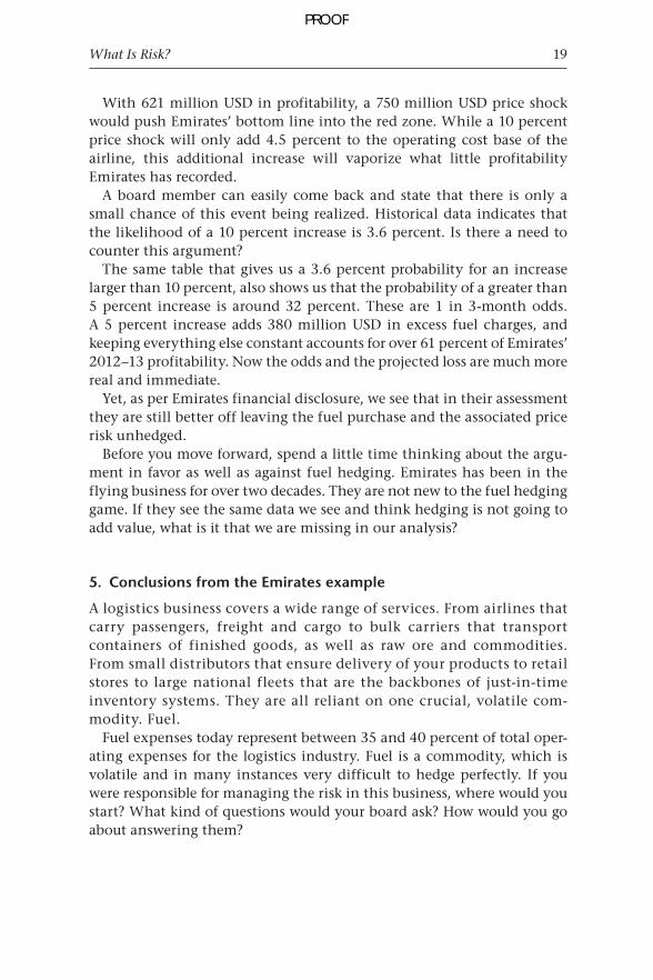
So what does Emirates sees that we are not seeing? To answer this ques-tion we have to revisit the jet fuel price and volatility graphs presented earlier. The first graph in Figure 18 shows price plot, while the second shows rolling volatility.

Emirates has two concerns.The first is that jet fuel prices are at historical highs. In their opinion,

at these levels the likelihood of prices going up is low. There is a much higher chance that prices will decline. If Emirates hedges its jet fuel expo-sure at current prices, fuel cost will be locked in at these levels, which would be especially painful if fuel prices were to collapse.

Emirates is not the only airline to feel this way. After the collapse of crude oil price in 2008, a number of regional airlines took a bath when

PROOF

What Is Risk? 21

their hedging strategies backfired by locking them in at peak price levels of 130 USD a barrel while the market tanked to 33 USD a barrel.

The second concern is volatility. While prices are at historical highs, volatility is at historical lows. The question is when (not if) volatility rises, will prices rise or decline? Emirates apparently feels that with the rise in volatility they are more likely to decline.

Given the above context, Emirates believes that until the picture about jet fuel clears up, they would be better off by partially passing on the cost increase to customers via fuel surcharges and adjustments. Such an approach is more flexible given the current context, and allows Emirates the option to hedge its exposure when prices can be locked at lower levels.

Hence Emirates’ decision to leave their jet fuel exposure unhedged in 2012–13.

Parting words

Remember the four questions.

What is the exposure?1. What is the trend for the exposure?2. What is the impact of risk factors on exposure?3. What is our risk appetite?4.

54

3

210

20.0%

15.0%

10.0%

5.0%

0.0%

May

-90

Apr

-91

Apr

-02

Mar

-92

Mar

-03

Feb

-93

Feb

-04

Jan-

94

Jan-

05

Dec

-94

Dec

-05

Nov

-06

Nov

-95

Oct

-96

Oct

-07

Sep

-08

Aug

-09

Jul-1

0Ju

n-11

May

-12

Apr

-13

Sep

-97

Aug

-98

Jul-9

9Ju

n-00

May

-01

Jun-

91

Jun-

92

Jun-

93

Jun-

94

Jun-

95

Jun-

96

Jun-

97

Jun-

98

Jun-

99

Jun-

00

Jun-

01

Jun-

02

Jun-

03

Jun-

04

Jun-

05

Jun-

06

Jun-

07

Jun-

08

Jun-

09

Jun-

10

Jun-

11

Jun-

12

Figure 18 Jet fuel prices and volatilities – 1990 to 2013

PROOF

22 Models at Work

As with everything else, a misdiagnosis followed by an incorrect prescrip-tion does more damage than good. You don’t want a flu shot when what you really need is a splint.

Annexure 1 – Building a histogram in EXCEL

The EXCEL Data Analysis Tool Pack comes with a powerful histogram tool that you can use to dissect distributions, prices and percentage returns.

A histogram is calculated on a series of daily price changes on a given financial security. Within risk terms we call daily price changes daily returns, and these returns could be positive or negative. The histogram in Figure 19 takes a daily return series, sorts the series and then slots each return in a given return bucket.

We will show how to build a simple histogram for the USD–EUR exchange rate.

Use the daily exchange rate series to calculate daily returns. Each return is calculated by the application of LN(P1/P0) where LN is the natural log function in EXCEL, P1 is the new exchange rate, P0 is the old exchange rate. This is approximately equal to the daily percentage price change in the underlying exchange rate.

We will take this return series and use it to calculate a histogram similar to the one in Figure 19.

You can find the histogram tool under the Data Analysis Tools tab in EXCEL. If for some reason you don’t see a Data Analysis Tools tab in your version of EXCEL, go to EXCEL Options, chose Add-ins and then simply add the Data Analysis Add-in to enable this tab (see Figure 21).

200

180

160

140

120

100

80

60

40

20

Bin

0

–25%

–23%

–22%

–20%

–18%

–16%

–14%

–13%

–11%–9

%–7

%–5

%–4

%–2

% 2% 4% 5%M

ore

0%0.00%

20.00%

40.00%

60.00%

Freq

uenc

y

80.00%

100.00%

120.00%

Frequency Cumulative %

Figure 19 Histogram

PROOF

What Is Risk? 23

To generate the histogram, select the daily return series as your input range. Opt for New Worksheet Ply, Cumulative Percentage and Chart Output (see Figure 22) to see a graphical representation of the histogram as well as a supporting frequency count table.

When you press Ok, EXCEL will create a new tab for you and show the histogram.

Figure 21 EXCEL’s data analysis functionality

Figure 20 USD –EUR daily returns

PROOF

24 Models at Work

Figure 22 EXCEL’s data analysis histogram functionality

60 120.00%

100.00%

80.00%

60.00%

50

40

30

Freq

uenc

y

20

10

Bin

–2.7

7%

–2.3

7%

–1.1

8%

–1.9

7%

–1.5

8%

–0.7

8%

–0.3

9%

–0.0

1%

–0.4

1%

–0.8

0%

–1.2

0%

–1.6

0%

–1.9

9%M

ore

0

40.00%

20.00%

0.00%

Frequency Cumulative %

Figure 23 Histogram of daily returns

PROOF

What Is Risk? 25

Figure 24 Frequency table output for histogram of daily returns

The histogram is a great summary of the entire distribution of prices. The worst-case daily price shock (the downside) in the histogram in Figure 23 is marked at −2.77 percent. The upside is about 1.99 percent

If I asked you what is the worst that can happen, you can easily tell me that my nightmarish scenario based on historical returns is a loss of over −2.77 percent (the extreme left corner on the bottom) if I am long (bought) Euro or a loss of over 1.99 percent if I am short (sold) Euro versus the US dollar.

My next two questions would be, over what time frame and with what odds?

The returns are calculated on a daily basis, hence the answer to the first question is over any given trading day.

The second answer requires a bit of work. There are approximately 181 days (frequency count) in the graph above (Figure 23). Your worst-case loss is a once in 181 days event. The probability of you seeing a loss greater than this number is 1/181 or 0.55 percent.

Luckily for us our EXCEL histogram output worksheet already includes a table with these probabilities and numbers in it, shown in Figure 24.

If you put all of the above material together, there is only a 0.55 percent chance that you will see a worst case loss of over −2.77 percent on any given trading day if you bought Euros, and a 1.1 percent chance that you will see a loss of over 1.99 percent if you sold Euros.

PROOF

26 Models at Work

Figure 25 Extract of data set

Annexure 2 – Trailing (rolling) correlations and volatilities

1. Rolling volatilities

Rolling or trailing volatilities analyze the trends in volatility over a period of time for a particular instrument or portfolio of instruments. They are graphical representations of how the riskiness of given instruments have changed over time, and depict the trend witnessed in risk levels. A rising trend indicates an increase in risk due to increased fluctuations in under-lying prices (level and/or frequency) over the period of study. A horizontal trend line indicates that average volatilities have remained stable over the period, whereas a declining trend line shows decreasing levels of risk.

It is calculated by obtaining price time series for the given instrument or portfolio. We have considered time series data for gold spot prices obtained from www.onlygold.com, silver spot prices (London PM fix in USD) from www.kitco.com, crude oil spot prices from www.eia.gov and the EUR−USD exchange rates from www.oanda.com for the period 1 January 2004 to 7 June 2013. See Figure 25 for an extract of this data set.

The daily return series is then calculated from the price data as the natural logarithm of the ratio of successive (consecutive) prices:

A series of daily volatilities for 90-day windows is determined on a roll forward basis, rolling forward a day at a time. The daily volatilities are cal-culated using EXCEL’s STDEV( ) function applied to 90 consecutive return observations.

⎛ ⎞⎟⎜ ⎟⎜ ⎟⎜ ⎟⎜⎝ ⎠–

lnPrice

Pricet

t 1

=

PROOF

What Is Risk? 27

The resulting volatility series is graphed in Figure 29 for gold, silver, crude oil (Brent and WTI) and the EUR–USD exchange rate.

A given point on the graph represents the daily volatility calculated using the past 90 returns available. Another way of presenting the results is to calculate an average of consecutive volatilities, again on a roll for-ward basis, as shown in Figure 30.

The graph in Figure 31 depicts the volatility trend line for a series of 60 volatility averages.

Figure 26 Calculation of daily returns

Figure 27 Calculation of 90-day daily volatilities (part 1)

Figure 28 Calculation of 90-day daily volatilities (part 2)

PROOF

28 Models at Work

0.00%

26/0

5/04

26/0

5/05

26/0

5/06

26/0

5/07

26/0

5/08

26/0

5/09

26/0

5/10

26/0

5/11

26/0

5/12

26/0

5/13

1.00%

2.00%

3.00%

4.00%

5.00%

6.00%

7.00%

8.00%

Gold Silver Crude oil – WTI Crude oil – Brent EUR–USD

Figure 29 90-day rolling volatilities for gold, silver, crude oil and EUR–USD

Figure 30 Calculation of 60-vol average rolling volatilities

PROOF

What Is Risk? 29

A given point on the graph represents the average of the previous 60 volatilities at that particular date.

Rolling forward a day at a time means that the periods for consecutive daily volatilities overlap. A large return would continue to impact the results until it dropped out of the 90-day window range. When using historical volatilities in calculations, it is more appropriate to use rolling volatilities that are calculated for discrete non-overlapping intervals, to remove the bias of previous intervals.

To determine non-overlapping discrete intervals we define the window length (90 days in Cell AL1), and the start row and final row references in the sheet. The latter two entries are the start and end cells of the date column for the returns section of the sheet.

For the first interval the end row reference is calculated as start row reference + window length − 1. For the following intervals the start row reference will be the previous end row + 1, while the end row will be the

0.00%

1.00%

2.00%

3.00%

4.00%

5.00%

6.00%

7.00%

19/0

8/04

19/0

8/05

19/0

8/06

19/0

8/07

19/0

8/08

19/0

8/09

19/0

8/10

19/0

8/11

19/0

8/12

Gold Silver Crude oil – WTI Crude oil – Brent EUR–USD

Figure 31 60-vol average rolling volatilities for gold, silver, crude oil and EUR–USD

Figure 32 Defining the start row for determining non-overlapping intervals for rolling volatilities

PROOF

30 Models at Work

minimum of the start row reference for that interval + window length − 1 and the final row reference.

In row 2, columns AN to AR, we specify the columns where the return series are present, that is, I to M. This will be used in identifying the inter-val range to be used in the calculations. For example, the formula in cell AN5, identifies the range “I5:I94” and calculates the standard deviation of the returns in this range (see Figure 34).

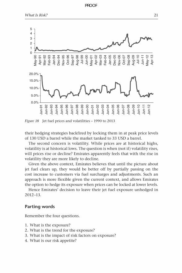
The volatility trend line using this methodology is given in Figure 35.Crude oil price daily volatilities peaked in early 2009, to over 6 percent

for WTI and over 5 percent for Brent. They have fallen to around 1 per-cent since then. Silver currently has the highest volatility among the

Figure 33 Defining the final row for determining non-overlapping intervals for rolling volatilities

Figure 34 Calculating rolling volatilities for non-overlapping intervals

PROOF

What Is Risk? 31

instruments considered here, while EUR–USD exchange rates have expe-rienced a flat, slightly declining, trend for the past 2 to 2.5 years.

2. Rolling correlations

A similar analysis was done with respect to correlations with gold price returns. The trend lines show how correlations of gold with each instru-ment in turn, silver, crude oil, EUR−USD, have varied over time.

Using the return series and EXCEL’s CORREL() function applied to the gold return series and another instrument’s series, the 90-day rolling cor-relations have been calculated in Figure 36.

0.00%

1.00%

2.00%

3.00%

4.00%

5.00%

6.00%

7.00%

01/0

5/04

01/0

9/04

01/0

1/05

01/0

5/05

01/0

9/05

01/0

1/06

01/0

5/06

01/0

9/06

01/0

1/07

01/0

5/07

01/0

9/07

01/0

1/08

01/0

5/08

01/0

9/08

01/0

1/09

01/0

5/09

01/0

9/09

01/0

1/10

01/0

5/10

01/0

9/10

01/0

1/11

01/0

5/11

01/0

9/11

01/0

1/12

01/0

5/12

01/0

9/12

01/0

1/13

01/0

5/13

Gold Silver Crude oil – WTI Crude oil – Brent EUR–USD

Figure 35 Rolling volatilities for non-overlapping discrete intervals

1

–0.40

26/0

5/04

26/0

5/05

26/0

5/06

26/0

5/07

26/0

5/08

26/0

5/09

26/0

5/10

26/0

5/11

26/0

5/12

26/0

5/13

–0.20

–

0.20

0.40

0.60

0.80

1.00

Silver Crude oil – WTI Crude oil – Brent EUR–USD

Figure 36 90-day rolling correlations

PROOF

32 Models at Work

Taking an average of the previous 60 correlations, a series of average rolling correlations is also determined in Figure 37.

–0.40

–0.20

–

0.20

0.40

0.60

0.80

1.00

19/0

8/04

19/0

8/05

19/0

8/06

19/0

8/07

19/0

8/08

19/0

8/09

19/0

8/10

19/0

8/11

19/0

8/12

Silver Crude oil – WTI Crude oil – Brent EUR–USD

Figure 37 60-correlations average rolling correlations

Figure 38 Calculating rolling correlations for non-overlapping intervals

To remove the bias of previous intervals on any given interval, a discrete non-overlapping interval rolling correlation series is also derived. A meth-odology similar to that for identifying discrete intervals for volatilities has been used. The formula at cell AU5 works out to “=CORREL($I5:$I94, $J5:$J94)”, as shown in Figure 38.

A graphical representation of the non-overlapping interval rolling cor-relations is given in Figure 39.

PROOF

What Is Risk? 33

–0.20 –0.10

–0.10 0.20 0.30 0.40 0.50 0.60 0.70 0.80 0.90

01

/05/

040

1/0

9/04

01

/01/

050

1/0

5/05

01

/09/

050

1/0

1/06

01

/05/

060

1/0

9/06

01

/01/

070

1/0

5/07

01

/09/

070

1/0

1/08

01

/05/

080

1/0

9/08

01

/01/

090

1/0

5/09

01

/09/

090

1/0

1/10

01

/05/

100

1/0

9/10

01

/01/

110

1/0

5/11

01

/09/

110

1/0

1/12

01

/05/

120

1/0

9/12

01

/01/

130

1/0

5/13

Silver Crude oil – WTI Crude oil – Brent EUR–USD

Figure 39 Rolling correlations for non-overlapping discrete intervals

PROOF

603

Index

absolute price charts, 10accountability, 164accrual swaps, 506, 555–60advanced fixed income securities,

529–68advanced products, 578–94AIG, see American International

Group (AIG)all or nothing options, 496aluminum, 363–4American International Group (AIG),

204–9American options, 236, 479, 484–6,

513–15amortizing swaps, 503, 504annualized return, 141–2annualized volatility, 142, 424–5antithetic variable technique, 256–8apparel, textiles and footwear prices, 396approximate method, for VaR, 83–4arbitrage free models, 228Asian options, 497, 521–2asset concentration limits, 130asset price, 238, 239, 481, 482asset quality ratio, 128asset swaps, 506assumptions

in financial institutions, 168validation of, 164

AUD-USD exchange rate, 329–34, 339–40

Australian dollar, gold and, 327–34automated exception tracking and

reporting, 163average strike options, 497

bank failures, 195–209Bank for International Settlement

(BIS), 38banking regulation

Basel I, 175–6Basel II, 176–81Basel III, 181–5comprehensive capital analysis and

review (CCAR), 185–7evolution of, 174–89Great Depression and, 174–5

reasons for ineffectiveness of, 187–9Regulation Q, 174–5

bank risk function, 162–4barrier options, 496–7, 523–5Basel I, 175–6Basel II, 176–81

ICAAP requirement, 178–81market discipline, 178minimum capital requirements, 177pillars of, 176–8supervisory review, 177–8

Basel III, 181–5liquidity reforms, 182–5market-related monitoring tools, 185

basis rate swaps, 503, 545–6basket options, 499Bear Stearns, 191, 195–9Bermuda option, 495beta, with respect to market indices,

144–5binary options, 496, 557–8binomial option pricing, 508–10binomial trees, 226–7, 510–11Black Scholes formula, 95, 98–9, 226–7

intuitive derivation of N(d2), 246–9for option pricing, 255–61, 516underlying assumptions, 247, 249

Black Scholes risk adjusted probabilities, 243–6

bond options, 493bonds

risk management, 65–6VaR for, 65–73yield to maturity (YTM), 565–8

bond yieldshistorical spreads in, 404–23inflation and, 404–16

breakeven analysis, 168Brent crude oil prices, 442, 443Broadie, Mark, 57building materials WPI, 403business events risk, 576

callable bonds, 493call options, 236, 237, 470–5, 479–80,

511–14call premium, 23, 519–20

PROOF

604 Index

cancellable swap, 506cap-floor parity, 554–5capital, 102, 169–70

diversified, 172economic, 171for liquidity risk, 194–5marginal, 172minimum capital requirements, 177regulatory, 172shortfall framework, 170sufficiency, 170types of, 172

capital adequacy ratio, 127–8capital estimation, for liquidity risk

management, 189–95capital guaranteed notes, 581–2capital loss limits, 112, 115–19capital market products, limits

applicable to, 129capital protected notes (CPNs), 581–2cap rate, 493–4caps, 553–4cash distributions, 239, 482cash flow mismatches, 130cash flows, 529

determining, 544–5discounting, 529–46matrix, 539–40

cash reserves, 190–4CCAR, see comprehensive capital

analysis and review (CCAR)central bank discount window, 190Central Bank Gold Agreement

(CBGA), 328central banks, risk systems for, 165–7China

coal, 452–3energy consumption, 448energy insights, 448–53gold demand from, 328–9natural gas, 450–1oil, 449–50

chooser options, 499, 523–5CIR (Cox Ingersoll Ross) model, 228–9,

300–3cleaning, laundry, and personal

appearance CPI, 399coal, 452–3coffee, 373–4coin tosses, 214collateralized debt obligations

(CDOs), 594comfort zone, 132

commodities3-sigma band for, 428–9annualized volatility, 424–5cash prices, 350correlations, 429–37correlations between, 350–80gold prices, 327–34, 335–49Monte Carlo simulation models

for, 220price volatility, 345price volatility trends, 424–37relative values, 338–44

commodity linked notes, 560–2, 582–3commodity swaps, 506composite options, 496compounding swaps, 503compound options, 498comprehensive capital analysis and

review (CCAR), 185–7concentration limits, 112, 130–1conditional VaR, 73, 86–8confidence levels, 110confirmation, 575constant maturity swaps, 504constant maturity treasury swaps, 504consumer price index (CPI), 391–400

composition of, 392crude oil prices and, 394–400inflation, 405–11, 412–16inflation and, 392

contagions, 168contingent liability limits, 131contractual maturity mismatch, 184convertibles, 493convexity, 123–4, 142–3copper, 366–7corn, 369–70, 389–90corn oil, 376–8correlation coefficient (r), 146–9, 352correlations, 350–80

aluminum, 363–4coffee, 373–4commodities, 429–37copper, 366–7corn, 369–70corn oil, 376–8cotton, 367–9crude palm oil, 379–80, 384diesel fuel, 355–6fuel oil, 354–5gold prices, 358–9natural gas, 357–8platinum, 361–3

PROOF

Index 605

correlations – continuedsilver, 360–1soybean oil, 378–9steel, 364–5sugar, 375–6West Texas crude oil, 352–3wheat No. 1, 372–3wheat No. 2, 370–2

CORREL() function, 31–3, 58, 62–4cotton, 367–9counterparty limits, 127coupon swaps, 542COVAR() function, 57–8Cox-Ingersoll-Ross (CIR) interest rate

model, 300–3credit approval, 159credit default swaps, 590–3credit management, 157–62credit policy, 158–9credit proposal, 157–8credit risk function, 156–63credit risk limits, 124–8cross-currency interest rate swaps, 503,

546–8cross currency swaps, 578crude oil, 442–6, 453–5, 457crude oil prices, 106–10, 269–70, 277–82,

303, 305–61995–2013, 320–1aluminum and, 363–4apparel, textiles and footwear prices

and, 396Brent prices, 338building materials WPI and, 403cleaning, laundry, and personal

appearance CPI and, 399coffee and, 373–4consumer price index and, 394–400copper and, 366–7corn and, 369–70corn oil and, 376–8correlations with other commodities,

350–80cotton and, 367–9crude palm oil and, 379–80diesel fuel and, 355–6drivers for projecting, 313–26education CPI and, 399equity market and, 317–19excess production capacity and,

314–15, 324–5excess supply and, 315–16, 324food and beverages prices and, 395

food prices and, 401fuel and lightning prices and, 397fuel oil and, 354–5futures contract spreads and, 319, 326gold and, 333–4gold prices and, 335–6, 337–41, 358–9household, furniture, and equipment

prices and, 397house rent and, 396inflation and, 391–403manufactures WPI and, 403Medicare CPI and, 400natural gas and, 357–8, 446–8outlook, 313–19in Pakistan, 458platinum and, 361–3recreation and entertainment prices

and, 398S&P 500 and, 320–2silver and, 360–1soybean oil and, 378–9steel and, 364–5sugar and, 375–6transport and communication prices

and, 398USD-EUR and, 322–3US dollar and, 317volatility, 426West Texas crude oil, 352–3wheat No. 1 and, 372–3wheat No. 2 and, 370–2wholesale price index (WPI) and,

400–3WTI, 323, 338, 339

crude palm oilfutures, 381–90prices, 350, 379–80

cumulative caps, 586–7cumulative probability distribution

percentage, 136currencies, Monte Carlo simulation

models for, 220currency swaps, 490

daily returns, 5–7, 27, 51daily time series data, 47daily VaR, 55–6, 60daily volatilities, 27data, risk management, 103–4default modeling, 97–9default term structure, 538–9deferred swaps, 503delta, 483

PROOF

606 Index

delta normal method, 71–3derivatives

advanced fixed income securities, 529–68

advanced products, 578–94building blocks, 473–5payoff profiles, 467–75pricing, 507–28products and pricing, 476–90template for evaluating, 477–90terminology, 463–75types of, 463–75variations, 491–506

descriptive and prescriptive school, 103diesel fuel, 355–6differential swaps, 505diffusion, 220–6digital options, 496discounting cash flows, 529–46distressed asset sales, 189distribution, 11distribution of returns, 40distribution plots, price volatility, 6diversified capital, 172Dodd-Frank Act, 187drift, 220–6duration, 142duration limits, 123–4

earnings/profitability ratios, 128economic capital, 171education CPI, 399embedded bond options, 493embedded risk function, 162Emirates airline, 14–21, 273–300employee stock options, 492–3energy insights, 438–59

China, 448–53coal, 452–3crude oil, 442–6, 457India, 453–6natural gas, 438–42, 450–1, 455–6,

457–9oil, 449–50Pakistan, 456–9US, 438–48

equilibrium models, 228equity, 98–9equity linked notes, 579–81equity market, crude oil prices and,

317–19equity swap, 505Euro, 12, 328, 345

eurodollar futures, 502European options, 236, 239–40, 249–53,

482–3, 511–13, 515–20European swap options, 495EUR-USD exchange rate, 12, 271–2, 328,

332, 336, 337, 345, 384–5EWMA, see exponentially weighted

moving average (EWMA)EXCEL

building histograms in, 22–5Monte Carlo simulators in, 213–61rolling correlations in, 31–3rolling volatilities in, 26–31

exception handling, 131–2exchange options, 499exercise/strike price, 236, 238–9, 243–4,

481–2exotic options, 495, 520–1exotics, 464expiration date, 236, 479exponentially weighted moving average

(EWMA), 41, 44calculation of variance, 54calculation of volatility, 54–5, 76–8daily VaR, 55determining volatility, 52–3weights used in, 53–4

exports, 306–7exposure

to risk, 12–16, 34trend for, 15–16

exposure limits, 112extendable swaps, 506extreme events, 39

factor sensitivities, 45–6fats and oils volatility, 428Federal Reserve, 186, 346–7fibers and textiles volatility, 427financial analysis ratios, 127–8financial institution (FI) limits, 127financial institutions

assumptions in, 168financial markets and, 168

financial markets, 1685-year treasury note futures, 502fixed currency swaps, 549fixed income securities, 529–68fixed swaps, 502floating currency swaps, 550–3floating swaps, 503, 542, 545–6floor-ceiling agreement, 495floors, 554

PROOF

Index 607

food prices, 393, 395, 401food volatility, 428foreign currency LCR, 185foreign currency options, 491foreign exchange products, limits

applicable to, 129forward contracts, 463–5, 467, 468–70,

473–5, 486–8, 500–1, 533–4forward curve, 542forward price, 487–8forward rate agreement (FRA),

500–1, 533forward rates, 530–1, 542, 544, 562–4forward start options, 499forward swaps, 503four eyes, 574fuel, lighting and lubricants WPI, 402fuel and lightning prices, 397fuel expenses, 14–21fuel hedging problem, 273–300

board requirement and recommendations, 277

case context and background, 273–7identifying relationships to be

examined, 276initial analysis and requirements,

274–5jet fuel price shock estimation, 289–90linking financial model to simulation,

282–7presenting case to client, 294–300shortfall using Monte Carlo

implementation, 290–4simulating crude oil prices, 277–82tweaking model, 287–9two black boxes, 275–6

fuel oil, 354–5full valuation approach, 82–3funding concentration, 184funding concentration limits, 130futures, crude palm oil, 381–90futures contracts, 463, 465–6, 467,

488–9, 501–2futures contract spreads, crude oil prices

and, 319, 326futures options, 492futures prices, 489

gamma, 483gap limits, 130gasoline prices, 444–5generator function, 215–16global economic outlook, 319–20

global financial crisis, 185, 327, 425global liquidity ratio adjustments, 182–4gold, motives for holding, 343–4gold demand, 328–9gold/oil ratio, 333–4gold prices, 265–6

2004–2013, 335Australian dollar and, 329–34crude oil prices and, 333–4, 335–6,

337–41, 358–9crude palm oil futures and, 386–7drivers, trends and future prospects,

327–9EUR-USD exchange rate and, 345gold to silver ratio and, 344–5, 347–9industrial commodities and, 342JPY-USD exchange rates and, 346other commodities and, 342–4relative values, 338–44

gold to silver ratio, 344–5, 347–9grains and feeds volatility, 427Great Depression, 174–5

Halton sequence, 258hedge funds

margin requirements for, 93–5PD for, 95–6portfolio volatility for, 91–2volatility distribution, 92–3

hedging, 34–5fuel hedging problem, 273–300

histogramsbuilding in EXCEL, 22–5daily return, for fuel oil, 7of volatility distribution, 9

historical returns, Monte Carlo simulation using, 229–36, 262–73

historical simulation method, 40, 42–3, 44, 78–80

historical spreads, in bond yields, 404–23

HJM (Heath, Jarrow & Merton), 228–9holding period return, 141household, furniture, and equipment

prices, 397house rent, 396Huygens, Christiaan, 170

ICAAP, see Internal Capital Adequacy Assessment Process (ICAAP)

impact, of risk, 13, 14, 16–18imports, 306incremental VaR, 73, 82–4

PROOF

608 Index

index options, 491–2India

crude oil, 453–5energy insights, 453–6natural gas, 455–6

Indian bond market, 404–23inflation, 309, 328

bond yields and, 404–16consumer price index (CPI), 405–11,

412–16crude oil prices and, 391–403impact of CPI components on, 392impact of WPI components on, 393in India, 411in Pakistan, 407–11wholesale price index (WPI), 405–6,

408–16yield to maturity (YTM), 565–8

Interbank Repurchase (Repo) contract, 190

interest rate caps, 493–4, 553–4interest rate collars, 495interest rate differential (IRD) trades, 585interest rate floors, 494, 554interest rate futures, 501–2interest rate options, 493interest rate return structure, 300–3interest rate risk, limits, 131interest rates

forward rates, 530–1, 562–4option pricing and, 239, 482simulating, 228–9spot rates, 530, 562–4term structure of, 532–3yield to maturity (YTM), 531–2

interest rate swaps (IRS), 489–90, 535–46Internal Capital Adequacy Assessment

Process (ICAAP), 177, 178–81internal/concentration limits, 128in-the-money options, 238intrinsic value, of option, 238inventory age limits, 112inventory losses projections, 110inverted curve instrument, 588

Jensen’s Alpha, 145–6jet fuel prices, 14–21, 289–90Jorian, Philippe, 38JP Morgan, 151JPY-USD exchange rates, 346

know-your-customer (KYC) procedures, 127

ladder options, 525–8LCR, 183LCR by significant currency, 185Lehman Brothers, 199–204less is more school, 102–3leverage, 189LIBOR-in-arrears swaps, 503limits

action plan for trigger zones, 132application to products, 129back testing, 138–40capital loss, 112, 115–19cash flow mismatches, 130concentration, 112, 130–1contingent liability, 131convexity, 123–4counterparty, 127credit risk, 124–8duration, 123–4exception handling, 131–2exposure, 112financial institution (FI), 127hierarchy of, 113–15interest rate risk, 131internal/concentration, 128inventory age, 112liquidity risk, 130–1market risk, 123–4maturity, 130operational, 111–12potential future exposure (PFE), 113pre-settlement risk (PSR), 113, 124–6PVBP, 124regulatory, 128regulatory approach, 122–3repricing, 131review of, 131review triggers, 138–40in risk management, 111–15sensitivity, 112setting, 111, 115–40settlement risk, 126–7stop loss, 37–8, 112, 115–19, 133–40transaction, 112VaR, 120–2

liquidity crises, 195–209liquidity-driven bank failures, 195–209liquidity ratios, 128liquidity reserves, 190–4liquidity risk

capital estimation for management of, 189–95

liquidity run crisis and, 191

PROOF

Index 609

liquidity risk – continuedmetrics for monitoring, 184–5

liquidity risk limits, 130–1liquidity run crisis, 191–2loans, post approval life cycle

of, 159–61logistics industry, 19–21long position, 236, 479long-term interest rates, 301–3look back options, 497–8, 522look back period, 46loss given default (LGD), 89

M2, 308–9management action trigger, 36manufactures WPI, 403marginal capital, 172marginal VaR, 73, 84–6margin lending, case study, 89–97margin requirements, 93–5margin shortfall analysis, 108–9market discipline, 178market-related monitoring tools, 185market risk, 153–6market risk limits, 123–4maturity date, 236, 479maturity limits, 130MC-Normal approach, 264MDURATION() function, 67Medicare CPI, 400Merton structured approach, 96, 97–9metrics, 106–10minimum capital requirements, 177models

risk, 151–3risk management, 103–4, 105–6

monetary policy rate decision, 303–10money market products, limits

applicable to, 129Monte Carlo simulation applications,

262–300fuel hedging problem, 273–300VaR using historical returns, 262–73

Monte Carlo simulation method, 40, 43, 44, 80–2

early days, 262–3fixing the distribution, 263historical returns and, 264–73option pricing using, 515–28

Monte Carlo simulators in Excel, 213–61about, 215binomial trees and, 226–7Black Scholes model, 226–7

Black Scholes risk adjusted probabilities and, 243–6

building your first, 216–20drift, diffusion, and volatility drag,

220–6European call option pricing using,

249–53extending to currencies and

commodities, 220interest rate simulation, 228–9introduction to, 213–14option pricing using, 236–61process or generator function,

215–16using historical returns, 229–36

moving average, for volatility, 8–9MYR-USD exchange rate, 385–6

name crisis, 191–2, 195–9natural gas, 357–8, 438–42, 446–8,

450–1, 455–6, 457–9net foreign asset (NFA), 304, 308Nielsen, Lars Tyge, 243NSFR, 183

oil, 449–50see also crude oil

oil prices, see crude oil pricesOPEC crude oil production, 443–4operational control risk, 576operational limits, 111–12operational risk, 177, 576option premium, 479option pricing, 481–6

American options, 513–15antithetic variable technique, 256–8barrier options, 523–5binomial, 508–10chooser options, 523–5convergence and variance reduction

techniques, 254–61elements of, 238–9European options, 239–40, 249–53,

511–13, 515–20in EXCEL, model framework, 240–3exercise/strike price, 236, 238–9,

243–4exotic options, 520–1ladder options, 525–8receipt of stock and N(d1), 244–6terminology, 236–40using Monte Carlo simulation, 236–61,

515–28

PROOF

610 Index

options, 464, 466, 468, 470–5, 479–86, 491–500

other metals volatility, 427outliers, 352out-of-the money options, 238

Pakistanbond market, 404–23comparative analysis with India,

416–23energy insights, 456–9inflation in, 391–403, 407–11monetary policy rate decision for,

303–10natural gas, 457–9oil production and consumption, 457price indices, 391–403

participating forwards, 578–9part term structure, 537payoff profiles, 467–75Pettis, Michael, 346plain vanilla interest rate swap, 489–90platinum, 361–3policy discount rate, 310portfolio return series, 74–5portfolio VaR, 56–64

calculation of, 58–64theoretical overview, 56–8

portfolio volatility, 91–2, 149–50post loan approval credit life cycle,

159–61potential future exposure (PFE)

limit, 113precious metals volatility, 426pre-settlement risk (PSR) limits, 113,

124–6price changes, 34price discovery, 576price indices

components of, 391–403consumer price index (CPI), 391–400wholesale price index (WPI), 391,

392–3price shocks, 289–90price VaR, 69–73price volatility, 4–9

in commodities, 345rolling volatilities, 26–31

pricing modelscrude oil prices, 313–26gold prices, 327–34gold-silver ratio, 335–49

probability of shortfall, 73, 88–9

profit margins, 290–4proprietary trading, 576put options, 236–8, 470–5, 479, 482–4,

513, 514–15put premium, 144puttable bonds, 493PVBP limits, 124

quantitative easing, 347quanto options, 496quanto swaps, 505, 585quasi-random sequences, 258–61

RAND() function, 233, 234, 279random noise, 280–1random sequences, 258rang accrual notes, 558–60range accruals, 583–4ranges, 589–90rate sensitive assets (RSA), 131rate sensitive liabilities (RSL), 131rate VaR, 68–9, 70–3raw materials WPI, 402recreation and entertainment prices, 398refined products volatility, 426Regulation Q, 174–5regulatory approach limits, 122–3regulatory capital, 172regulatory limits, 128regulatory risk, 576relative pricing, 507relative values, 338–44remittances, 307–8repricing limits, 131reserve currencies, 345–7return series, 49–51, 74–5rho, 484risk

definitions of, 3exposure to, 12–16, 34impact, 13, 14, 16–18models, 151–3operational, 177, 576price volatility and, 4–9survival of, 162understanding, 11ways of thinking about, 3–4, 12–14

risk appetite, 18–19risk assessment, 11–12risk audits, 163–4risk factors, 13, 14

correlations between, 44–5risk functions, 151–2, 162–4

PROOF

Index 611

risk management, 3, 39, 100–50bonds, 65–6data and models, 103–4framework, 13, 100–1, 115limits and control process, 111–15liquidity, 189–95metrics and sensitivities, 106–10models and tools, 105–6objective of, 39risk policy, 101–3setting limits, 115–40systems, 151–67treasury, 154–6

risk measurement, 34–99target accounts, 34–8value at risk (VaR), 37–99

risk metrics, 141–50risk neutral probabilities, 507risk policy, 101–3risk reporting process, 114risk sensitivities, 45–6risk survival information flow

design, 164risk systems

assessment framework, 162–4building, 151–67for central banks, 165–7credit risk function, 156–63risk survival information flow

design, 164treasury and market risk, 153–6

rolling correlations, 31–3rolling volatilities, 9, 26–31

S&P 500, 320–2safe haven currencies, 345–7scaling weights, 53–4scatter plots, 351–2sensitivity limits, 112settlement, 576settlement risk limits, 126–7Sharpe ratio, 143–4short position, 236short rates, 531short-term interest rates, 300–1, 302–3shout options, 500silver

crude oil prices and, 360–1gold to silver ratio, 344–5, 347–9

silver prices, 267–8, 350simple moving average (SMA), 41, 51,

52–3, 55, 57, 75simulation applications, 262–300

forecasting monetary policy rate decision for Pakistan, 303–10

fuel hedging problem, 273–300interest rate return structure, 300–3

SMA, see simple moving average (SMA)Society for Worldwide Interbank

Financial Telecommunications (SWIFT), 575

soybean oil, 378–9spot rates, 530, 562–4standard deviation/volatility (Vol), 141statutory liquidity reserves (SLR), 190–4STDEV() function, 26, 75steel, 364–5steepener/flattener notes, 587–8step-up swaps, 503stock index futures, 501stock options, 491stop loss limits, 37–8, 112, 115–19,

133–40stress testing, 163–4, 168–74, 187

capital and, 170–3framework, 169–74

stress zone, 132strike price, 236, 238–9sugar, 375–6supervisory review, 177–8swaps, 464, 489–90, 502–6, 534–46,

546–62, 590–4switchables, 584synthetic configurations, 473–5synthetic forward contract, 500systems risk, 576

Taleb, Nicholas Nassim, 38, 106, 109, 215

target accounts, 34–8characteristics of, 36definition of, 36forms of, 36–7management action and, 37–8

target liquid reserves, 130theta, 483–4

3-sigma band, 428–9ticket approval, 574ticket authorization, 574ticket verification, 574time series data, 47–8, 49time to expiration, of option, 239, 482tools, risk management, 105–6total return swaps, 593–4transaction risk, 576transaction limits, 112

PROOF

612 Index

transport and communication prices, 398

treasury bill futures, 502treasury bond futures, 501treasury function, 569–77treasury note futures, 502treasury rates, 537treasury risk, 153–6Treynor ratio, 145trigger zones, 132troubled asset relief program

(TARP), 185two-dimensional binomial tree, 510–11

uncertainty, 11, 13underwriting, 159unencumbered assets, 184unit diffusion, 222–4unit drift, 222–4US banking regulation, 185–7US crude oil demand and supply, 444US dollar, 12, 327–8

AUD-USD exchange rate, 329–34, 339–40

crude oil prices and, 317depreciation of, 336EUR-USD exchange rate, 12, 271–2,

328, 332, 336, 337, 345, 384–5JPY-USD exchange rates, 346MYR-USD exchange rate, 385–6outlook for, 320revaluation of, 321–2, 336weakness of, 345–7

US energy insights, 438–48crude oil, 442–6natural gas, 438–42

US gasoline prices, 444–5US Treasury Daily Yield Curve, 48US Treasury interpolated interest

rates, 48

value at risk (VaR), 37–99, 105–6application case study, 89–97approximation to, 83–4for bonds, 65–73calculation of, 46–64, 65–90caveats for, 43–5conditional, 73, 86–8daily, 55–6, 60definition of, 39–40delta normal method, 71–3full valuation approach, 82–3

historical simulation method, 42–3, 44, 78–80

holding period, 56incremental, 73, 82–4introduction to, 38–46limits, 120–2marginal, 73, 84–6methodology, 46–51methods, 40–3Monte Carlo simulation method, 43,

44, 80–2portfolio, 56–64price, 69–73probability of shortfall, 73, 88–9rate, 68–9, 70–3risk or factor sensitivities, 45–6using historical returns, 262–73variance/covariance (VCV) approach,

44, 51–3, 56–8, 60–4, 75–8variance/covariance method, 41–2

vanilla call or put options, 521VaR, see value at risk (VaR)VAR() function, 57–8variance, 39variance/covariance (VCV) approach, 40,

41–2, 44, 51–3, 56–8, 60–4, 75–8variance reduction techniques, 254–61variance swap, 505vega, 484volatility

annualized, 142, 424–5of asset price, 239, 482calculation of, 105commodity prices, 424–37crude palm oil futures, 383daily, 27portfolio, 91–2, 149–50price, 4–9, 345rolling, 26–31

volatility distribution, 92–3volatility drag, 220–6volatility index, 11volatility swap, 505volatility trend analysis, 150

warning zone, 132warrants, 492West Texas crude oil, 352–3West Texas Intermediate (WTI), 443

crude palm oil futures and, 387–8price indices and, 393

wheat No. 1, 372–3

PROOF

Index 613

wheat No. 2, 370–2, 388–9wholesale price index (WPI), 391, 392–3

composition of, 393crude oil prices and, 400–3inflation, 405–6, 408–16inflation and, 393

yield to maturity (YTM), 531–2, 565–8

zero coupon rates, 541, 543–4zero curve, 539, 540–1zero diffusion, 221–2zero drift, 221–3

PROOF

PROOF