continuity properties of the solution map for the generalized reduced ostrovsky equation

J. Differential Equations 252 (2012) 3797–3815

Contents lists available at SciVerse ScienceDirect

Journal of Differential Equations

www.elsevier.com/locate/jde

Continuity properties of the solution mapfor the generalized reduced Ostrovsky equation

Melissa Davidson

Department of Mathematics, University of Notre Dame, Notre Dame, IN 46556, United States

a r t i c l e i n f o a b s t r a c t

Article history:Received 5 August 2011Revised 11 November 2011Available online 25 November 2011

MSC:primary 35Q53

Keywords:Generalized reduced Ostrovsky equationOstrovsky equationShort pulse equationVakhnenko equationCauchy problemSobolev spacesWell-posednessNonuniform dependence on initial dataApproximate solutionsHölder continuity

It is shown that the data-to-solution map for the generalizedreduced Ostrovsky (gRO) equation is not uniformly continuouson bounded sets in Sobolev spaces on the circle with exponents > 3/2. Considering that for this range of exponents the gROequation is well posed with continuous dependence on initial data,this result makes the continuity of the solution map an optimalproperty. However, if a weaker Hr-topology is used then it isshown that the solution map becomes Hölder continuous in Hs .

© 2011 Elsevier Inc. All rights reserved.

1. Introduction and results

We consider the initial value problem for the generalized reduced Ostrovsky equation (gRO)

∂t u + 1

k + 1∂x

(uk+1) − γ ∂−1

x u = 0, (1.1)

u(x,0) = u0(x), x ∈ T, t ∈ R, (1.2)

E-mail address: [email protected].

0022-0396/$ – see front matter © 2011 Elsevier Inc. All rights reserved.doi:10.1016/j.jde.2011.11.013

http://dx.doi.org/10.1016/j.jde.2011.11.013

http://www.ScienceDirect.com/

http://www.elsevier.com/locate/jde

mailto:[email protected]

http://dx.doi.org/10.1016/j.jde.2011.11.013

3798 M. Davidson / J. Differential Equations 252 (2012) 3797–3815

where k is a positive integer, γ is a constant, T = R/2πZ is the torus, and Hs(T) is the Sobolev spaceon the torus with exponent s. For s > 3/2 we prove that the Cauchy problem (1.1)–(1.2) is locallywell posed in Hs(T) and that the data-to-solution map is continuous but not uniformly continuous.Furthermore, we show that the solution map is Hölder continuous in Hs(T) if it is equipped with anHr(T)-norm, 0 � r < s.

The gRO equation appears in the literature more often in the following local form

(ut + ukux

)x = γ u. (1.3)

When k = 1 this equation is obtained from the Ostrovsky equation found in Ostrovsky [20]

(ut + c0ux + αuux + βuxxx)x = γ u. (1.4)

By choosing β = 0, the equation is called the reduced Ostrovsky equation in Cai, Xie, and Yang [2],in Parkes [21] and in Stepanyants [27]. With c0 = 0 = β and α = 1 = γ , it is called the Ostrovsky–Hunter equation by Boyd [1] and the Vakhnenko equation by Morrison, Parkes and Vakhnenko [19]and Vakhnenko and Parkes [32]. This equation was first presented by Vakhnenko [31] to describehigh-frequency waves in a relaxing medium. Furthermore, it has been shown to be integrable inthe sense that an inverse scattering problem can be formulated [32]. Hunter [13] noted that writingthe equation as (1.4) meant that there is no long wave dispersion. The equation would now modelwaves with a wave frequency that is significantly larger than the Coriolis frequency. A numericalsolution was then found with an initial guess of a sine wave for the lowest amplitude wave. Huntershowed that the equation is well posed if the initial condition and the corresponding solution u(x, t)are mean zero. An exact N loop soliton solution was found for an arbitrary integer N � 2 in [19].A transformation of the independent variables enabled the use of Hirota’s method. The solution wasthen found in its implicit form. In Boyd [1], it is noted that the dilational symmetry of the Ostrovsky–Hunter equation allows a restriction to the torus without loss of generality. Since the equation hastraveling wave and limiting wave properties that are found in other wave equations, they are used infinding a solution. The method of matched asymptotic expansions is used to find an approximationand the derived approximations are then tested for accuracy.

For k = 2 this equation becomes the short pulse equation (SPE). It is used in nonlinear optics asa model for very short pulse propagation in nonlinear media by Schäfer and Wayne [25]. It has beenshown that the SPE provides a better approximation to the solution of Maxwell’s equation than thenonlinear Schrödinger equation (NLSE). Sakovich and Sakovich discovered that the SPE is integrable aswell by finding a Lax pair and then transforming the equation into the sine-Gordon equation [23]. Thisallowed the authors then to show it has explicit analytical solutions of loop and breather form [24].Global well-posedness with small initial data was shown in Pelinovsky and Sakovich [22]. Studying theSPE under its guise as the Ostrovsky–Hunter equation, Liu, Pelinovsky and Sakovich found sufficientconditions for wave breaking on an infinite line and in a periodic domain [18]. Local well-posednessfor s � 2 was shown and conditions for wave breaking are found that are sharper than previous re-sults. From an applications standpoint, the accuracy of the SPE increases as the pulse width shortens.This has led to the derivation of a regularized SPE which has smooth traveling wave solutions, underappropriate conditions by Costanzino, Manukian and Jones [4].

Well-posedness for the Ostrovsky equation (γ �= 0) has been presented in many sources. We con-sider a few here and refer the reader to the references of the papers for further study. Local-in-timewell-posedness for Hs(R), s > 3/2, was proved using parabolic regularization while continuous de-pendence came from Bona–Smith approximations in Varlamov and Liu [33]. This result was extendedto s > 3/4 in Linares and Milanés [17]. The result was further extended for s � −1/8 locally andglobally to L2(R) by Huo and Jia [14]. Using a variation of Bourgain’s called the “I-method”, globalwell-posedness in Hs(R) for s > −3/10 is shown in Isaza and Mejía [15]. Other well-posedness resultsare presented in [7,30,34].

M. Davidson / J. Differential Equations 252 (2012) 3797–3815 3799

The first result of our work states that the periodic initial value problem for the gRO equationis well posed in the sense of Hadamard in Sobolev spaces with exponent greater than 3/2. Moreprecisely, we have the following result.

Theorem 1.1. If s > 3/2 and u0 ∈ Hs(T) then there exist T > 0 and a unique solution u ∈ C([0, T ]; Hs(T)) ofthe initial value problem (1.1)–(1.2), which depends continuously on the initial data u0 . Furthermore, we havethe estimate

∥∥u(t)∥∥

Hs(T)� k

√2 · ecs T · ‖u0‖Hs(T), for 0 � t � T � 1

2kcsln

(1 + 1

‖u0‖kHs(T)

), (1.5)

where cs > 0 is a constant depending on s.

Well-posedness of the gRO equation on the line and for s > 3/2 has been proved by Stefanov,Shen and Kevrekidis [26]. Also, in [26] they proved some global well-posedness results. The proofof Theorem 1.1 is based on a Galerkin-type approximation method, which for quasi-linear symmetrichyperbolic systems can be found in Taylor [28,29].

The second result of this paper, which is motivated by the works of Himonas and Holliman [8],Himonas and Kenig [9], Himonas, Kenig and Misiołek [10], Himonas, Misiołek and Ponce [11], andHolliman [12], demonstrates that continuous dependence of the solution on initial data is sharp.

Theorem 1.2. If s > 3/2 then the data-to-solution map for the generalized reduced Ostrovsky equation de-fined by the Cauchy problem (1.1)–(1.2) is not uniformly continuous from any bounded subset of H s(T) intoC([0, T ]; Hs(T)).

The proof of the analogous result for the Camassa–Holm equation relies on the conservation ofthe H1-norm [9,10], while the proof of the corresponding result for the Degasperis–Procesi equationrelies on the conservation of a twisted L2-norm [8]. However, the method of the proof for Theo-rem 1.2 does not invoke any conserved quantities as in Grayshan [6]. To demonstrate the sharpnessof continuity, sequences of approximate solutions that contain terms of both high and low frequencyare constructed. The actual solutions are then found by solving the Cauchy problem with initial datagiven by the approximate solutions at time t = 0. Then the error produced by solving the Cauchyproblem and by using approximate solutions is shown to be inconsequential. The proof is also basedon the well-posedness result Theorem 1.1 and in particular on estimate for the size of the solutionand its lifespan.

We note that our method of proof of well-posedness does not rely upon a fixed point theorem forcontraction mappings. Since there is not uniform continuity on the space where the solutions live,the local well-posedness of gRO in Hs(T) cannot be shown by use of this method.

Although the data-to-solution map is not uniformly continuous on Hs(T), in our third result weshow that if a properly weakened topology is chosen then it becomes Hölder continuous. More pre-cisely, we prove the following result.

Theorem 1.3. Let s > 3/2 and 0 � r < s. Then the data-to-solution map of the Cauchy problem for the gener-alized reduced Ostrovsky equation (1.1)–(1.2) is Hölder continuous with exponent

α ={

1, if 0 � r � s − 1,

s − r, if s − 1 < r < s(1.6)

as a map from B(0,ρ) ⊂ Hs(T), with Hr(T)-norm, into C([0, T ]; Hr(T)). More precisely, we have

∥∥u(t) − w(t)∥∥

r � c∥∥u(0) − w(0)

∥∥αr (1.7)
C([0,T ];H (T)) H (T)


for all u(0), w(0) ∈ B(0,ρ) = {u ∈ Hs(T): ‖u‖Hs(T) < ρ} and u(t), w(t) the solutions corresponding to theinitial data u(0), w(0), respectively. The lifespan T > 0 and the constant c > 0 depend on s, r and ρ .

The proof of Theorem 1.3 follows the work of Chen, Liu, and Zhang [3] and Grayshan [6]. Thepaper is structured as follows. In Section 2, we define the inverse partial and approximate solutions,estimate the Hσ (T) norm of the error, and construct sequences of initial data that demonstrate thenon-uniformity of the data-to-solution map. In Section 3, we provide an overview of the local well-posedness result for s > 3/2 with an accompanying solution size estimate. Finally, in Section 4, weprove Theorem 1.3.

2. Proof of Theorem 1.2

Before giving the proof of the non-uniform dependence for the gRO equation we shall state thedefinition of the inverse ∂−1

x and its basic properties. A more detailed discussion of ∂−1x can be found

in Fokas and Himonas [5] and Holliman [12]. For f ∈ Hs(T) the inverse of ∂x is defined by the formula

∂−1x f (x)

.= ∂−1x f (x) − 1

2π

2π∫0

∂−1y f (y)dy, (2.1)

where ∂−1x is given by

∂−1x f (x)

.=x∫

0

f (y)dy − x

2π

2π∫0

f (y)dy.

It defines a continuous linear map ∂−1x : Hs(T) → H s+1(T) satisfying the estimate∥∥∂−1

x f∥∥

H s+1(T)� ‖ f ‖H s(T) � ‖ f ‖Hs(T). (2.2)

Also, it is both a left and right inverse of the operator ∂x : H s+1(T) → H s(T). Moreover, it satisfies therelations

∂−1x ∂x f (x) = f (x) − f (0), f ∈ Hs(T),

∂x∂−1x f (x) = f (x) − 1

2πf (0), f ∈ Hs(T).

Since for any r � 0 and g ∈ Hr(T) we have ‖g‖Hr(T) � 2r/2‖ f ‖Hr (T) , from (2.2) we also obtain thefollowing inequality ∥∥∂−1

x f∥∥

Hr(T)� 2r/2

∥∥∂−1x f

∥∥Hr(T)

� 2r/2‖ f ‖Hr−1(T). (2.3)

Recall that for any real number s the Sobolev space Hs(T) is defined by the norm

‖ f ‖2Hs(T) = 1

2π

∑k∈Z

(1 + k2)s∣∣ f (k)

∣∣2.

The homogeneous Sobolev space H s(T) is the subspace of Hs(T) defined by the condition f (0) = 0and its norm is defined by


‖ f ‖2H s(T)

=∑k∈Z

|k|2s∣∣ f (k)

∣∣2,

where Z = Z − {0}. Here, the Fourier transform is defined by

f (k) =∫T

e−ixk f (x)dx.

Next, we will prove Theorem 1.2 for Sobolev exponents s > 3/2. The basis of our proof rests uponfinding two sequences of solutions, {un}, {vn} in C([0, T ]; Hs(T)), to the gRO i.v.p. (1.1)–(1.2) thatshare a common lifespan and satisfy

∥∥un(t)∥∥

Hs(T)+ ∥∥vn(t)

∥∥Hs(T)

� 1,

limn→∞

∥∥un(0) − vn(0)∥∥

Hs(T)= 0,

and

lim infn

∥∥u1,n(t) − u−1,n(t)∥∥

Hs(T)�

∣∣sin(t)∣∣ for t ∈ (0, T ] for k-odd,

lim infn

∥∥u1,n(t) − u0,n(t)∥∥

Hs(T)�

∣∣sin(t/2)∣∣ for t ∈ (0, T ] for k-even.

2.1. Approximate gRO solutions

For any n, a positive integer, we define the approximate solution uω,n = uω,n(x, t) as

uω,n(x, t).= ωn−1/k + n−s cos(nx − ωt), (2.4)

where

ω = −1,1 if k is odd and ω = 0,1 if k is even. (2.5)

Then substituting the above approximate solutions into gRO (1.1) gives the error

E(t) = E = ωn−s sin(nx − ωt)

+ [ωn−1/k + n−s cos(nx − ωt)

]k · [−n−s+1 sin(nx − ωt)]

+ γ ∂−1x

[uω,n]. (2.6)

Taking into account that for ω satisfying condition (2.5) we have ωk = ω; thus, the first term in theerror, which has Hs norm of 1, cancels. Therefore, we have

E = −k∑

j=1

(k

j

)ωk− jn− 1

k (k− j)− js−s+1 cos j(nx − ωt) sin(nx − ωt) + γ ∂−1x

[uω,n].


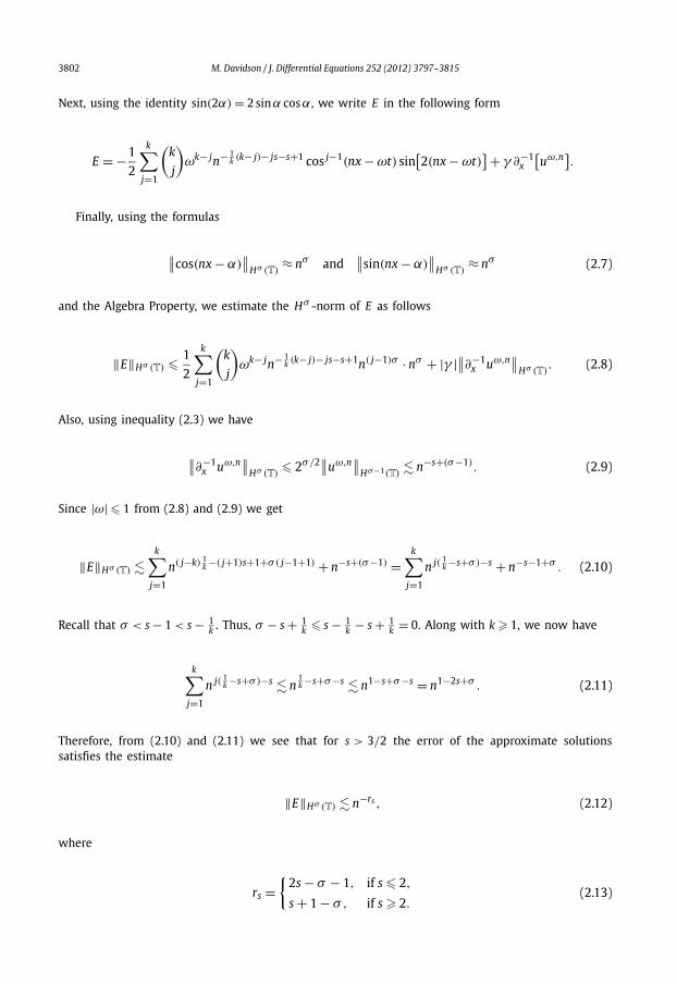
Next, using the identity sin(2α) = 2 sinα cosα, we write E in the following form

E = −1

2

k∑j=1

(k

j

)ωk− jn− 1

k (k− j)− js−s+1 cos j−1(nx − ωt) sin[2(nx − ωt)

] + γ ∂−1x

[uω,n].

Finally, using the formulas

∥∥cos(nx − α)∥∥

Hσ (T)≈ nσ and

∥∥sin(nx − α)∥∥

Hσ (T)≈ nσ (2.7)

and the Algebra Property, we estimate the Hσ -norm of E as follows

‖E‖Hσ (T) � 1

2

k∑j=1

(k

j

)ωk− jn− 1

k (k− j)− js−s+1n( j−1)σ · nσ + |γ |∥∥∂−1x uω,n

∥∥Hσ (T)

. (2.8)

Also, using inequality (2.3) we have

∥∥∂−1x uω,n

∥∥Hσ (T)

� 2σ/2∥∥uω,n

∥∥Hσ−1(T)

� n−s+(σ−1). (2.9)

Since |ω| � 1 from (2.8) and (2.9) we get

‖E‖Hσ (T) �k∑

j=1

n( j−k) 1k −( j+1)s+1+σ ( j−1+1) + n−s+(σ−1) =

k∑j=1

n j( 1k −s+σ )−s + n−s−1+σ . (2.10)

Recall that σ < s − 1 < s − 1k . Thus, σ − s + 1

k � s − 1k − s + 1

k = 0. Along with k � 1, we now have

k∑j=1

n j( 1k −s+σ )−s � n

1k −s+σ−s � n1−s+σ−s = n1−2s+σ . (2.11)

Therefore, from (2.10) and (2.11) we see that for s > 3/2 the error of the approximate solutionssatisfies the estimate

‖E‖Hσ (T) � n−rs , (2.12)

where

rs ={

2s − σ − 1, if s � 2,

s + 1 − σ , if s � 2.(2.13)


2.2. Actual gRO solutions

Let uω,n(x, t) be the actual solutions to the gRO i.v.p. (1.1)–(1.2) with initial data uω,n(x,0) =uω,n(x,0). More precisely, uω,n(x, t) solves

∂t uω,n = −ukω,n∂xuω,n + γ ∂−1

x uω,n, (2.14)

uω,n(x,0) = ωn−1/k + n−s cos(nx), x ∈ T, t ∈ R. (2.15)

Notice that (2.7) implies that the initial data uω,n(x,0) ∈ Hs(T) for all s � 0, since

∥∥uω,n(·,0)∥∥

Hs(T)� ωn−1/k + n−s

∥∥cos(nx)∥∥

Hs(T)≈ 1,

for n sufficiently large. Hence, by Theorem 1.1, there is a T > 0 such that for n > 1, the Cauchyproblem (2.14)–(2.15) has a unique solution in C([0, T ]; Hs(T)) with lifespan T > 0 such that uω,n

satisfies (1.5) for t ∈ [0, T ].To estimate the difference between the actual solutions and the approximate solutions, we define

v = uω,n − uω,n which satisfies the following i.v.p.

∂t v = E −[

1

k + 1∂x

(uω,n)k+1 − 1

k + 1∂x(uω,n)

k+1]

+ γ ∂−1x v,

where

v(x,0) = 0, x ∈ T, t ∈ R.

For ease of notation, we rewrite the i.v.p. as

∂t v = E − 1

k + 1∂x[w · v] + γ ∂−1

x v, (2.16)

where

w = (uω,n)k + (

uω,n)k−1uω,n + · · · + uω,n(uω,n)

k−1 + (uω,n)k

and E satisfies the estimate in (2.12).We will now show that the Hs norm of the difference v decays to zero as n goes to infinity. Apply

the operator Dσ to both sides of (2.16), multiply by Dσ v , and integrate over the torus to get

1

2

d

dt

∥∥v(t)∥∥2

Hσ (T)=

∫T

Dσ E Dσ v dx (2.17)

− 1

k + 1

∫T

Dσ ∂x(w · v)Dσ v dx (2.18)

+ γ

∫T

Dσ ∂−1x v Dσ v dx. (2.19)

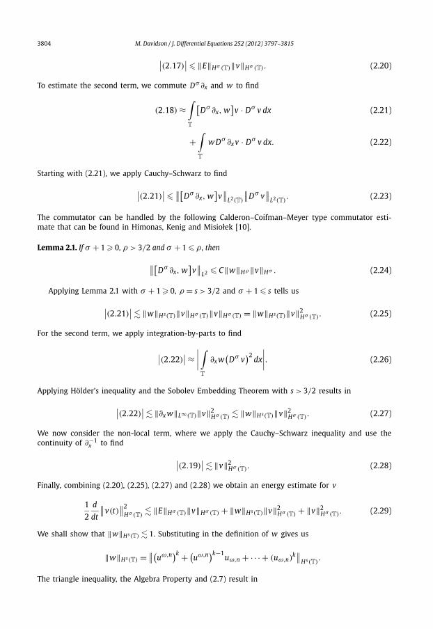
Applying the Cauchy–Schwarz inequality to the first integral, we get (2.17)

∣∣(2.17)∣∣ � ‖E‖Hσ (T)‖v‖Hσ (T). (2.20)
To estimate the second term, we commute Dσ ∂x and w to find

(2.18) ≈∫T

[Dσ ∂x, w

]v · Dσ v dx (2.21)

+∫T

w Dσ ∂x v · Dσ v dx. (2.22)

Starting with (2.21), we apply Cauchy–Schwarz to find∣∣(2.21)∣∣ �

∥∥[Dσ ∂x, w

]v∥∥

L2(T)

∥∥Dσ v∥∥

L2(T). (2.23)

The commutator can be handled by the following Calderon–Coifman–Meyer type commutator esti-mate that can be found in Himonas, Kenig and Misiołek [10].

Lemma 2.1. If σ + 1 � 0, ρ > 3/2 and σ + 1 � ρ , then∥∥[Dσ ∂x, w

]v∥∥

L2 � C‖w‖Hρ ‖v‖Hσ . (2.24)

Applying Lemma 2.1 with σ + 1 � 0, ρ = s > 3/2 and σ + 1 � s tells us∣∣(2.21)∣∣ � ‖w‖Hs(T)‖v‖Hσ (T)‖v‖Hσ (T) = ‖w‖Hs(T)‖v‖2

Hσ (T). (2.25)

For the second term, we apply integration-by-parts to find

∣∣(2.22)∣∣ ≈

∣∣∣∣ ∫T

∂x w(

Dσ v)2

dx

∣∣∣∣. (2.26)

Applying Hölder’s inequality and the Sobolev Embedding Theorem with s > 3/2 results in∣∣(2.22)∣∣ � ‖∂x w‖L∞(T)‖v‖2

Hσ (T) � ‖w‖Hs(T)‖v‖2Hσ (T). (2.27)

We now consider the non-local term, where we apply the Cauchy–Schwarz inequality and use thecontinuity of ∂−1

x to find ∣∣(2.19)∣∣ � ‖v‖2

Hσ (T). (2.28)

Finally, combining (2.20), (2.25), (2.27) and (2.28) we obtain an energy estimate for v

1

2

d

dt

∥∥v(t)∥∥2

Hσ (T)� ‖E‖Hσ (T)‖v‖Hσ (T) + ‖w‖Hs(T)‖v‖2

Hσ (T) + ‖v‖2Hσ (T). (2.29)

We shall show that ‖w‖Hs(T) � 1. Substituting in the definition of w gives us

‖w‖Hs(T) = ∥∥(uω,n)k + (

uω,n)k−1uω,n + · · · + (uω,n)

k∥∥

Hs(T).

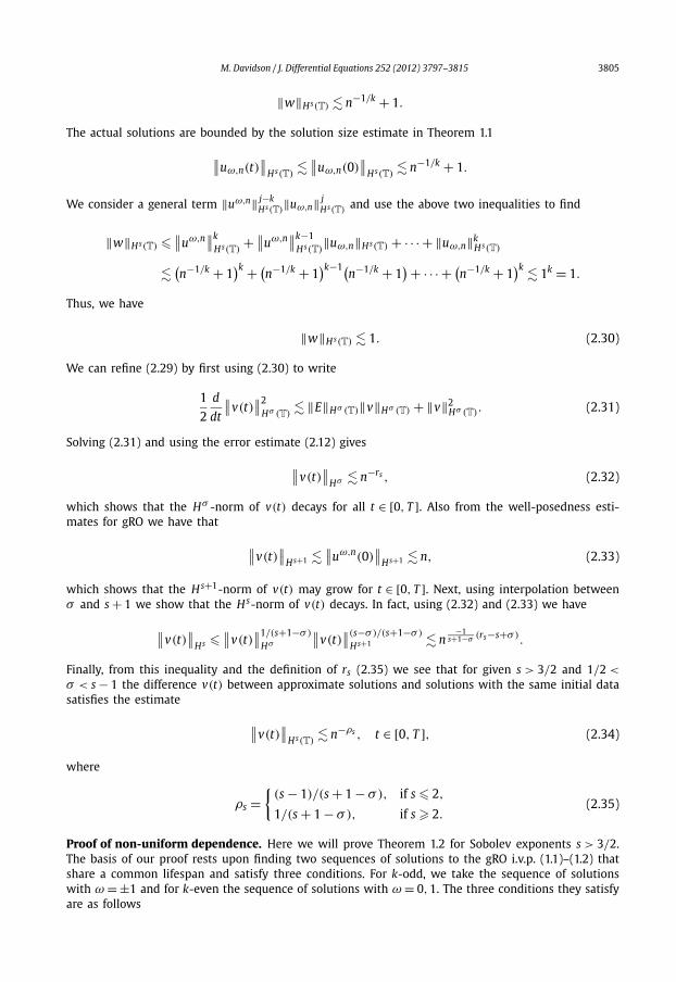
The triangle inequality, the Algebra Property and (2.7) result in


‖w‖Hs(T) � n−1/k + 1.

The actual solutions are bounded by the solution size estimate in Theorem 1.1∥∥uω,n(t)∥∥

Hs(T)�

∥∥uω,n(0)∥∥

Hs(T)� n−1/k + 1.

We consider a general term ‖uω,n‖ j−kHs(T)

‖uω,n‖ jHs(T)

and use the above two inequalities to find

‖w‖Hs(T) �∥∥uω,n

∥∥kHs(T)

+ ∥∥uω,n∥∥k−1

Hs(T)‖uω,n‖Hs(T) + · · · + ‖uω,n‖k

Hs(T)

�(n−1/k + 1

)k + (n−1/k + 1

)k−1(n−1/k + 1

) + · · · + (n−1/k + 1

)k � 1k = 1.

Thus, we have

‖w‖Hs(T) � 1. (2.30)

We can refine (2.29) by first using (2.30) to write

1

2

d

dt

∥∥v(t)∥∥2

Hσ (T)� ‖E‖Hσ (T)‖v‖Hσ (T) + ‖v‖2

Hσ (T). (2.31)

Solving (2.31) and using the error estimate (2.12) gives∥∥v(t)∥∥

Hσ � n−rs , (2.32)

which shows that the Hσ -norm of v(t) decays for all t ∈ [0, T ]. Also from the well-posedness esti-mates for gRO we have that ∥∥v(t)

∥∥Hs+1 �

∥∥uω,n(0)∥∥

Hs+1 � n, (2.33)

which shows that the Hs+1-norm of v(t) may grow for t ∈ [0, T ]. Next, using interpolation betweenσ and s + 1 we show that the Hs-norm of v(t) decays. In fact, using (2.32) and (2.33) we have∥∥v(t)

∥∥Hs �

∥∥v(t)∥∥1/(s+1−σ )

Hσ

∥∥v(t)∥∥(s−σ )/(s+1−σ )

Hs+1 � n−1

s+1−σ (rs−s+σ ).

Finally, from this inequality and the definition of rs (2.35) we see that for given s > 3/2 and 1/2 <

σ < s − 1 the difference v(t) between approximate solutions and solutions with the same initial datasatisfies the estimate ∥∥v(t)

∥∥Hs(T)

� n−ρs , t ∈ [0, T ], (2.34)

where

ρs ={

(s − 1)/(s + 1 − σ), if s � 2,

1/(s + 1 − σ), if s � 2.(2.35)

Proof of non-uniform dependence. Here we will prove Theorem 1.2 for Sobolev exponents s > 3/2.The basis of our proof rests upon finding two sequences of solutions to the gRO i.v.p. (1.1)–(1.2) thatshare a common lifespan and satisfy three conditions. For k-odd, we take the sequence of solutionswith ω = ±1 and for k-even the sequence of solutions with ω = 0,1. The three conditions they satisfyare as follows


(1) ‖uω,n(t)‖Hs(T) � 1 for t ∈ [0, T ],(2) ‖u1,n(0) − u−1,n(0)‖Hs(T) → 0 as n → ∞ for k-odd,

‖u1,n(0) − u0,n(0)‖Hs(T) → 0 as n → ∞ for k-even, and(3) lim infn ‖u1,n(t) − u−1,n(t)‖Hs(T) � |sin(t)| for t ∈ (0, T ] for k-odd,

lim infn ‖u1,n(t) − u0,n(t)‖Hs(T) � |sin(t/2)| for t ∈ (0, T ] for k-even.

Property (1) for k-even or odd follows from the solution size estimate in Theorem 1.1. We have∥∥uω,n(t)∥∥

Hs(T)�

∥∥uω,n(0)∥∥

Hs(T)� 1.

Property (2), for k-odd, follows from the definition of our approximate solutions (2.4). We have∥∥u1,n(0) − u−1,n(0)∥∥

Hs(T)= ∥∥u1,n(0) − u−1,n(0)

∥∥Hs(T)

= ∥∥n−1/k + n−s cos(nx) + n−1/k − n−s cos(nx)∥∥

Hs(T)

= 4πn−1/k → 0 as n → ∞.

Similarly, for k-even we have∥∥u1,n(0) − u0,n(0)∥∥

Hs(T)= ∥∥u1,n(0) − u0,n(0)

∥∥Hs(T)

= ∥∥n−1/k + n−s cos(nx) − n−s cos(nx)∥∥

Hs(T)

= 2πn−1/k → 0 as n → ∞.

For property (3), we consider k-odd first. Using the reverse triangle inequality we get∥∥u1,n(t) − u−1,n(t)∥∥

Hs �∥∥u1,n(t) − u−1,n(t)

∥∥Hs − ∥∥u1,n(t) − u1,n(t)

∥∥Hs − ∥∥u−1,n(t) − u−1,n(t)

∥∥Hs

�∥∥u1,n(t) − u−1,n(t)

∥∥Hs − n−ρs ,

from which we obtain that

lim infn→∞

∥∥u1,n(t) − u−1,n(t)∥∥

Hs � lim infn→∞

∥∥u1,n(t) − u−1,n(t)∥∥

Hs . (2.36)

Since, by the trigonometric identity cos(α − β) − cos(α + β) = 2 sinα sinβ , we have

u1,n(t) − u−1,n(t) = 2n1/k + 2n−s sin(nx) sin(t),

inequality (2.36) gives

lim infn→∞

∥∥u1,n(t) − u−1,n(t)∥∥

Hs(T)� lim inf

n→∞(∣∣sin(t)

∣∣ − n1/k) �∣∣sin(t)

∣∣, (2.37)

which completes the proof of property (3) in the case that k is odd.We now consider k-even. Similarly, using the reverse triangle inequality, the definition of approxi-

mate solutions, and the fact that the difference between solutions and approximate solutions decays,we get

lim inf∥∥u1,n(t) − u0,n(t)

∥∥Hs � lim inf

∥∥u1,n(t) − u0,n(t)∥∥

Hs , (2.38)
n→∞ n→∞


where now

u1,n(t) − u0,n(t) = n1/k + 2n−s sin(nx − t/2) sin(t/2).

Therefore (2.38) gives

lim infn→∞

∥∥u1,n(t) − u0,n(t)∥∥

Hs(T)� lim inf

n→∞(∣∣sin(t/2)

∣∣ − n1/k) �∣∣sin(t/2)

∣∣, (2.39)

which completes the proof of Theorem 1.2. �3. Proof of Theorem 1.1

The generalized reduced Ostrovsky equation (1.1) (as is) cannot be thought of as an o.d.e. on thespace Hs(T). Specifically, we note that for u ∈ Hs(T) the product uk∂xu ∈ Hs−1(T). This difficulty isovercome by showing the existence of solutions to a mollified smooth version of the gRO i.v.p., whichwe later show gives rise to solutions of (1.1)–(1.2). Consider the mollified smooth version of the gROi.v.p.

∂t u = − Jε[( Jεu)k · ∂x Jεu

] + γ ∂−1x u := Fε, (3.1)

u(x,0) = u0(x), u0 ∈ Hs(T), x ∈ T, t ∈ R, (3.2)

where for each ε ∈ (0,1], the operator Jε is the Friedrichs mollifier. We fix a Schwartz functionj ∈ S(R) that satisfies 0 � j(ξ) � 1 for every ξ ∈ R and j(ξ) = 1 for ξ ∈ [−1,1]. This allows us todefine the periodic functions jε as

jε(x) = 1

2π

∑n∈Z

j(εn)einx.

Then Jε is given by Jε f (x) = jε ∗ f (x). This construction of jε results in a lemma that will proverepeatedly useful throughout the paper.

Lemma 3.1. If r � s and I − Jε : Hs → Hr , then

‖ f − Jε f ‖Hr = o(εs−r). (3.3)

Proof. Let f ∈ Hs(T), then applying Hr(T) norm to (I − Jε) f gives us

limε→0

‖ f − Jε f ‖2Hr(T)

ε2(s−r)= lim

ε→0

∑k∈Z

(1 + k2)r | f (k)|2|1 − j(εk)|2ε2(s−r)

� limε→0

∑k∈Z|εk|>1

∣∣1 − j(εk)∣∣2∣∣ f (k)

∣∣2(1 + k2)s = 0. �

Using the Algebra Property, we see that the mollified i.v.p. is an o.d.e. on Hs(T). Moreover, foreach ε ∈ (0,1], the map Fε : Hs(T) → Hs(T) in (3.1) is continuously differentiable with the derivativeat u0 ∈ Hs(T) given by

F ′ε(u0)u = − Jε

(k( Jεu0)

k−1 Jεu · ∂x Jεu0 + ( Jεu0)k · ∂x Jεu

) + γ ∂−1x u.

Hence, for each ε ∈ (0,1], (3.1)–(3.2) has a unique solution uε with lifespan Tε > 0.


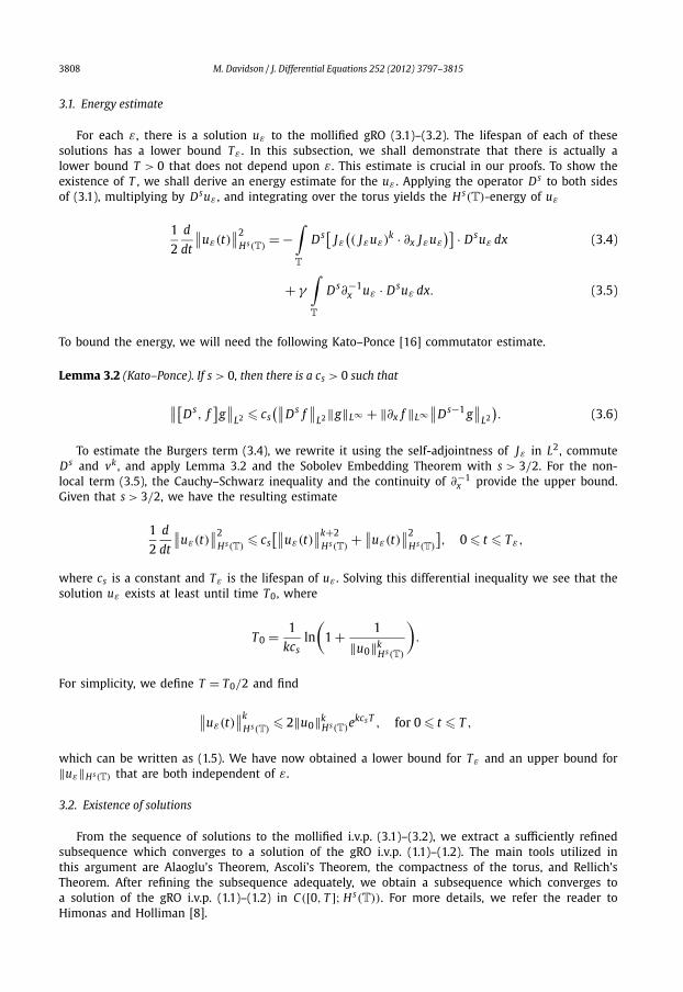
3.1. Energy estimate

For each ε, there is a solution uε to the mollified gRO (3.1)–(3.2). The lifespan of each of thesesolutions has a lower bound Tε . In this subsection, we shall demonstrate that there is actually alower bound T > 0 that does not depend upon ε. This estimate is crucial in our proofs. To show theexistence of T , we shall derive an energy estimate for the uε . Applying the operator Ds to both sidesof (3.1), multiplying by Dsuε , and integrating over the torus yields the Hs(T)-energy of uε

1

2

d

dt

∥∥uε(t)∥∥2

Hs(T)= −

∫T

Ds[ Jε(( Jεuε)

k · ∂x Jεuε

)] · Dsuε dx (3.4)

+ γ

∫T

Ds∂−1x uε · Dsuε dx. (3.5)

To bound the energy, we will need the following Kato–Ponce [16] commutator estimate.

Lemma 3.2 (Kato–Ponce). If s > 0, then there is a cs > 0 such that

∥∥[Ds, f

]g∥∥

L2 � cs(∥∥Ds f

∥∥L2‖g‖L∞ + ‖∂x f ‖L∞

∥∥Ds−1 g∥∥

L2

). (3.6)

To estimate the Burgers term (3.4), we rewrite it using the self-adjointness of Jε in L2, commuteDs and vk , and apply Lemma 3.2 and the Sobolev Embedding Theorem with s > 3/2. For the non-local term (3.5), the Cauchy–Schwarz inequality and the continuity of ∂−1

x provide the upper bound.Given that s > 3/2, we have the resulting estimate

1

2

d

dt

∥∥uε(t)∥∥2

Hs(T)� cs

[∥∥uε(t)∥∥k+2

Hs(T)+ ∥∥uε(t)

∥∥2Hs(T)

], 0 � t � Tε,

where cs is a constant and Tε is the lifespan of uε . Solving this differential inequality we see that thesolution uε exists at least until time T0, where

T0 = 1

kcsln

(1 + 1

‖u0‖kHs(T)

).

For simplicity, we define T = T0/2 and find

∥∥uε(t)∥∥k

Hs(T)� 2‖u0‖k

Hs(T)ekcs T , for 0 � t � T ,

which can be written as (1.5). We have now obtained a lower bound for Tε and an upper bound for‖uε‖Hs(T) that are both independent of ε.

3.2. Existence of solutions

From the sequence of solutions to the mollified i.v.p. (3.1)–(3.2), we extract a sufficiently refinedsubsequence which converges to a solution of the gRO i.v.p. (1.1)–(1.2). The main tools utilized inthis argument are Alaoglu’s Theorem, Ascoli’s Theorem, the compactness of the torus, and Rellich’sTheorem. After refining the subsequence adequately, we obtain a subsequence which converges toa solution of the gRO i.v.p. (1.1)–(1.2) in C([0, T ]; Hs(T)). For more details, we refer the reader toHimonas and Holliman [8].


3.3. Uniqueness

Here we will show the solution to the gRO i.v.p. (1.1)–(1.2) is unique. Our strategy is to develop anenergy estimate for the difference of two solutions. Fix the initial data u0 ∈ Hs(T) and let u and w betwo solutions to the gRO i.v.p. (1.1)–(1.2) with u(x,0) = u0(x) = w(x,0) ∈ Hs(T). Then the differencev = u − w satisfies the following Cauchy problem

∂t v = − 1

k + 1∂x

((u − w) ·

k∑j=0

u j wk− j

)+ γ ∂−1

x v,

with initial data v(0) = 0. For convenience, let w = ∑kj=0 u j wk− j . Then we have

∂t v = − 1

k + 1∂x(v w) + γ ∂−1

x v. (3.7)

Let σ ∈ [0, s − 1]. The Hσ (T)-energy estimate is then given by

1

2

d

dt‖v‖2

Hσ (T) = − 1

k + 1

∫T

Dσ ∂x(v w) · Dσ v dx + γ

∫T

Dσ ∂−1x v · Dσ v dx. (3.8)

To bound (3.8), we commute Dσ ∂x and w , which results in two integrals. The commutator integralis estimated by applying the Cauchy–Schwarz inequality followed by Lemma 2.1 and the solution sizeestimate (1.5). The second integral is bounded using integration by parts, the Sobolev EmbeddingTheorem and the solution size bound (1.5). The non-local term is estimated by the Cauchy–Schwarzinequality and the continuity of ∂−1

x . The resulting energy estimate is

1

2

d

dt

∥∥v(t)∥∥2

Hσ (T)�

∥∥v(t)∥∥2

Hσ (T), (3.9)

which we solve to find the inequality

∥∥v(t)∥∥2

Hσ (T)�

∥∥v(0)∥∥2

Hσ (T)e2cs T .

We recall that v = u − w where u and w are both solutions to the gRO i.v.p. (1.1)–(1.2). This meanswe have

∥∥v(t)∥∥

Hσ (T)�

∥∥v(0)∥∥

Hσ (T)ecs T

� ‖u0 − u0‖Hσ (T)ecs T = 0. (3.10)

Thus, we have uniqueness. �3.4. Continuity of the data-to-solution map

Proposition 3.3. The data-to-solution map for the gRO i.v.p. (1.1)–(1.2) from Hs(T) to C([0, T ]; Hs(T)) givenby u0 �→ u is continuous.


Proof. Fix u0 ∈ Hs(T) and let {u0,n} ⊂ Hs(T) be a sequence such that

limn→∞ u0,n = u0 in Hr(T).

Then if u is the solution to the gRO i.v.p. (1.1)–(1.2) with initial data u0 and if un is the solution tothe gRO i.v.p. with initial data u0,n , we will prove that

limn→∞ un = u, in C

([0, T ]; Hs).Our approach is to use energy estimates. To avoid some of the difficulties of estimating the terminvolving uk∂xu, we will use the Jε convolution operator to smooth out the initial data. Let ε ∈ (0,1].We take uε to be the solution to the gRO i.v.p. with smoothed initial data Jεu0 = jε ∗ u0. Similarly,let uε

n be the solution with initial data Jεu0,n . Applying the triangle inequality, we arrive at

‖u − un‖C([0,T ];Hs) �∥∥u − uε

∥∥C([0,T ];Hs)

+ ∥∥uε − uεn

∥∥C([0,T ];Hs)

+ ∥∥uεn − un

∥∥C([0,T ];Hs)

. (3.11)

We will prove that for any η > 0, there exists an N such that for all n > N , each of these terms canbe bounded by η/3 for suitable choices of ε and N . We note that the choice of a sufficiently small εwill be independent of N and will only depend on η; whereas, the choice of N will depend on bothη and ε. However, after ε has been chosen, N can be chosen so as to force each of the three terms tobe small.

3.4.1. Estimation of ‖uε − uεn‖C([0,T ];Hs(T))

We can bound this term directly using an Hs(T)-energy estimate. Let v = v(n, ε) = uε − uεn . Then

v satisfies the following Cauchy problem

∂t v = − 1

k + 1∂x

[(uε − uε

n

) k∑j=0

(uε

) j(uε

n

)k− j

]+ γ ∂−1

x (v),

where v(0) = uε(0) − uεn(0) = Jεu0 − Jεu0,n . For ease of notation, define

w =k∑

j=0

(uε

) j(uε

n

)k− j(3.12)

and we can write

∂t v = − 1

k + 1∂x(v w) + γ ∂−1

x v. (3.13)

Apply the operator Ds to both sides of (3.13), multiply by Ds v and integrate over the torus to obtainthe Hs(T)-energy

1

2

d

dt

∥∥v(t)∥∥2

Hs(T)= − 1

k + 1

∫T

Ds∂x(v w) · Ds v dx (3.14)

+ γ

∫Ds∂−1

x v · Ds v dx. (3.15)

T


To estimate (3.14), we commute Ds∂x and w and apply Lemma 2.1 and the Sobolev Embedding theo-rem to get

∣∣(3.14)∣∣ � ‖w‖Hs+1(T)‖v‖2

Hs(T). (3.16)

We shall consider ‖w‖Hs+1(T) . From our construction of Jε , we can see that our initial dataJεu0, Jεu0,n ∈ C∞ . Therefore, we may apply our solution size estimate (1.5), in conjunction with theAlgebra Property for s + 1 > 1/2, to the definition of ‖w‖Hs+1(T) to find

‖w‖Hs+1(T) �k∑

j=0

‖ Jεu0‖ jHs+1(T)

‖ Jεu0,n‖k− jHs+1(T)

.

In examining ‖ Jεu0‖Hs+1(T) we shall use that if f ∈ Hs+1(T), then

‖ f ‖Hs+1(T) � ‖ f ‖Hs(T) + ‖∂x f ‖Hs(T).

Using this inequality and ‖∂x Jε f ‖Hs(T) � αε ‖ f ‖Hs(T) , we can write

‖ Jεu0‖Hs+1(T) � ‖ Jεu0‖Hs(T) + ‖∂x Jεu0‖Hs(T) � 1

ε.

Similarly, we have

‖ Jεu0,n‖Hs+1(T) � 1

ε‖u0‖Hs(T) � 1

ε.

Therefore, we have

(3.16) � 1

ε‖v‖2

Hs(T). (3.17)

Now we consider the non-local term (3.15). Using the Cauchy–Schwarz inequality and the continuityof ∂−1

x results in

∣∣(3.15)∣∣ � ‖v‖2

Hs(T). (3.18)

Combining (3.17) and (3.18), we have the following energy estimate

1

2

d

dt

∥∥v(t)∥∥2

Hs(T)� 1

ε‖v‖2

Hs(T), (3.19)

which implies

∥∥v(t)∥∥2

Hs(T)�

∥∥v(0)∥∥2

Hs(T)e2 cs

ε t = ∥∥uε0 − uε

0,n

∥∥2Hs(T)

e2 csε t .

Recalling that the solutions are mollified, we write

∥∥uε0 − uε

0,n

∥∥s e

csε T = ∥∥ Jε

(uε

0 − uε0,n

)∥∥s e

csε T � ‖u0 − u0,n‖Hs(T)e

csε T .
H (T) H (T)


When we bound the first and third terms of (3.11), we will force ε to be small. After ε (independentof N) is chosen, we can bound ‖uε − uε

n‖C([0,T ];Hs(T)) by taking N large enough that

‖u0 − u0,n‖Hs(T) <η

3e− cε T

ε .

Then we have

∥∥uε − uεn

∥∥C([0,T ];Hs(T))

� η

3.

3.4.2. Estimation of ‖uε − u‖C([0,T ];Hs(T)) and ‖uεn − un‖C([0,T ];Hs(T))

Since the arguments will be largely the same for both terms, we will omit the subscript n untilsuch a time as differences in their handlings emerge. For convenience, let v = uε −u. We use Newton’sBinomial and the product rule to write

∂t v = 1

k + 1

[k+1∑j=1

(k + 1

j

)(−1) j j

(uε

)k+1− jv j−1∂x v (3.20)

+k+1∑j=1

(k + 1

j

)(−1) j(k + 1 − j)

(uε

)k− jv j∂xuε

](3.21)

+ γ ∂−1x v, (3.22)

with initial condition v0 = Jεu0 − u0.As in previous arguments, our strategy is to prove an Hs(T)-energy estimate for v . To bound the

terms that arise from the generalized Burgers equation, we consider an arbitrary term within the sum.We rewrite each term as a commutator and then apply the Cauchy–Schwarz inequality before usingLemma 3.2, the Sobolev Embedding Theorem, and the Algebra Property. For the non-local terms, weemploy the Cauchy–Schwarz inequality and the continuity of ∂−1

x . The resulting energy estimate is

1

2

d

dt‖v‖2

Hs(T) �k+1∑j=1

(∥∥uε∥∥k− j+1

Hs(T)‖v‖ j+1

Hs(T)

+ ∥∥uε∥∥k− j

Hs(T)

∥∥uε∥∥

Hs+1(T)‖v‖ j

Hs−1(T)‖v‖Hs(T) + ‖v‖2

Hs(T)

). (3.23)

By interpolating between 0 and s, we have

‖v‖Hs−1(T) � ‖v‖1s

H0(T)‖v‖1− 1

sHs(T)

� ‖v‖1s

L2(T).

Note that the solution size estimate (1.5) implies that ‖v(t)‖Hs(T) � 1. By utilizing an L2-energy es-timate, it can be shown that ‖v(t)‖L2(T) = o(εs). This is used to reduce the energy estimate to thedifferential inequality

dy � y + δ,
dt


where y = y(t) = ‖v(t)‖2Hs(T)

and δ = δ(ε) → 0 as ε → 0. Integrating from 0 to t , with t ∈ [0, T ], wehave

y(t) � y(0)eT + δ(eT − 1

).

3.4.3. Case of y = ‖v(t)‖Hs(T)

We first note that

∥∥v(t)∥∥

Hs(T)= ‖ Jεu0 − u0‖Hs(T) + δ(ε).

We can make δ arbitrary small by our choice of ε. Since

‖ Jεu0 − u0‖Hs(T) = o(εs−s) = o(1),

we have that ‖v(t)‖Hs(T) → 0 as ε → 0. Therefore, if we choose ε sufficiently small, we can boundthe first term of (3.11) by η

3 .

3.4.4. Case of y = ‖vn(t)‖Hs(T)

We first note that

∥∥vn(t)∥∥

Hs(T)= ‖ Jεu0,n − u0,n‖Hs(T) + δ(ε).

Thus, we have

‖ Jεu0,n − u0,n‖Hs(T) + δ �∥∥ Jε(u0,n − u0)

∥∥Hs(T)

+ ‖ Jεu0 − u0‖Hs(T) + ‖u0,n − u0‖Hs(T) + δ

� ‖u0,n − u0‖Hs(T) + ‖ Jεu0 − u0‖Hs(T) + δ.

We pick ε small so that ‖ Jεu0 − u0‖Hs(T) + δ(ε) is bounded. Then we pick n (dependent on ε) largeso that

∥∥uεn − un

∥∥Hs(T)

� ‖u0,n − u0‖Hs(T) + ‖ Jεu0 − u0‖Hs(T) + δ(ε) <η

3

for n sufficiently large and ε sufficiently small.This completes our proof of the well-posedness Theorem 1.1. �

4. Proof of Theorem 1.3

In this section, we will prove that the solution map for the gRO i.v.p. (1.1)–(1.2) is Hölder con-tinuous. We begin with the case 0 � r � s − 1, where s > 3/2. Let u0, w0 ∈ B(0,ρ) ⊂ Hs(T) andu, w ∈ C([0, T ]; Hs(T)) denote the corresponding solutions to the gRO i.v.p. (1.1)–(1.2) with initial datau0, w0, respectively. Notice that we can find a common lifespan T > 0 for all initial data u0 ∈ B(0,ρ).This follows from the fact that the lifespan Tu of any solution u ∈ B(0,ρ) to gRO (1.1)–(1.2) satisfiesthe following inequality

Tu � 1

2kcsln

(1 + 1

‖u0‖Hs(T)

)>

1

2kcsln

(1 + 1

ρ

)= T ,

where T does not depend upon u.


We need to show that there exist constant c and Hölder exponent α such that∥∥u(t) − w(t)∥∥

C([0,T ];Hr(T))� c‖u0 − w0‖α

Hr(T).

If we let v(t) = u(t) − w(t), then v satisfies the following energy estimate

1

2

d

dt

∥∥v(t)∥∥2

Hr(T)�

∥∥v(t)∥∥2

Hr(T),

as shown in the proof of uniqueness, see (3.9), provided that r ∈ [0, s − 1].Solving the differential inequality (3.10) gives∥∥u(t) − w(t)

∥∥Hr(T)

� ecs T ‖u0 − w0‖Hr(T), 0 � t � T , (4.1)

where u0, w0 ∈ B(0,ρ). Thus, we have shown that the data-to-solution map is Lipschitz continuousas a map

Hs(T) ⊃ B(0,ρ)with Hr -norm

→ C([0, T ]; Hr(T)

)for 0 � r � s − 1.

Let s − 1 < r < s, where s > 3/2. Interpolating between s − 1 and s we have

∥∥v(t)∥∥

Hr(T)�

∥∥v(t)∥∥s−r

Hs−1(T)

∥∥v(t)∥∥r+1−s

Hs(T). (4.2)

Since for s − 1 we can apply inequality (4.1), we have∥∥v(t)∥∥

Hs−1(T)� ecs T ‖u0 − w0‖Hs−1(T). (4.3)

Also, using the solution size estimate (1.5), we have∥∥v(t)∥∥

Hs(T)� k

√2 · ecs T (‖u0‖Hs(T) + ‖w0‖Hs(T)

)� k

√2 · ecs T · 2ρ. (4.4)

Combining (4.2), (4.3), and (4.4) gives∥∥v(t)∥∥

Hr(T)� ecs T ·(s−r)( k

√2 · ecs T · 2ρ

)r+1−s‖u0 − w0‖s−rHs−1(T)

.

Finally, taking into consideration the fact that s − 1 < r from the last inequality we obtain∥∥u(t) − w(t)∥∥

Hr(T)� cr,T ,ρ‖u0 − w0‖s−r

Hr(T), 0 � t � T ,

which shows that the solution map is Hölder continuous with exponent s − r. �Acknowledgments

The author would like to thank her advisor, Alex Himonas, for constructive conversations aboutthis paper and the Department of Mathematics at the University of Notre Dame for supporting herdoctoral studies. Also, she would like to thank the referee for helpful suggestions that led to improve-ments of this paper.


References

[1] J. Boyd, Ostrovsky and Hunter’s generic wave equation for weakly dispersive waves: matched asymptotic and pseudospec-tral study of the paraboloidal waves (corner and near-corner waves), European J. Appl. Math. 16 (2005) 65–81.

[2] J. Cai, S. Xie, C. Yang, Two loop soliton solutions to the reduced Ostrovsky equation, Int. Math. Forum 3 (2008) 1529–1536.[3] R.M. Chen, Y. Liu, P. Zhang, The Hölder continuity of the solution map to the b-family equation in weak topology, preprint.[4] N. Costanzino, V. Manukian, C. Jones, Solitary waves of the regularized short pulse and Ostrovsky equations, SIAM J. Math.

Anal. 41 (2009) 2088–2106.[5] A. Fokas, A. Himonas, Well-posedness of an integrable generalization of the nonlinear Schrodinger equation on the circle,

Lett. Math. Phys. 96 (2011) 169–189.[6] K. Grayshan, Continuity properties of the data-to-solution map for the periodic b-family equation, Differential Integral

Equations 25 (2012) 1–20.[7] G. Gui, Y. Liu, On the Cauchy problem for the Ostrovsky equation with positive dispersion, Comm. Partial Differential

Equations 32 (2007) 1895–1916.[8] A. Himonas, C. Holliman, On well-posedness of the Degasperis–Procesi equation, Discrete Contin. Dyn. Syst. 31 (2011)

469–488.[9] A. Himonas, C. Kenig, Non-uniform dependence on initial data for the CH equation on the line, Differential Integral Equa-

tions 22 (2009) 201–224.[10] A. Himonas, C. Kenig, G. Misiołek, Non-uniform dependence for the periodic CH equation, Comm. Partial Differential Equa-

tions 35 (2010) 1145–1162.[11] A. Himonas, G. Misiołek, G. Ponce, Non-uniform continuity in H1 of the solution map of the CH equation, Asian J. Math. 11

(2007) 141–150.[12] C. Holliman, Non-uniform dependence and well-posedness for the periodic Hunter–Saxton equation, J. Diff. Int. Eq. 23

(2010) 1150–1194.[13] J. Hunter, Numerical solutions of some nonlinear dispersive wave equations, Lect. Appl. Math. 26 (1990) 301–316.[14] Z. Huo, Y. Jia, Low-regularity solutions for the Ostrovsky equation, Proc. Edinb. Math. Soc. 49 (2006) 87–100.[15] P. Isaza, J. Mejía, Global Cauchy problem for the Ostrovsky equation, Nonlinear Anal. 67 (2007) 1482–1503.[16] T. Kato, G. Ponce, Commutator estimates and the Euler and Navier–Stokes equations, Comm. Pure Appl. Math. 41 (7) (1988)

891–901.[17] F. Linares, A. Milanés, Local and global well-posedness for the Ostrovsky equation, J. Differential Equations 222 (2006)

325–340.[18] Y. Liu, D. Pelinovsky, A. Sakovich, Wave breaking in the Ostrovsky–Hunter equation, SIAM J. Math. Anal. 42 (2010) 1967–

1985.[19] A.J. Morrison, E.J. Parkes, V.O. Vakhnenko, The N loop soliton solution of the Vakhnenko equation, Nonlinearity 12 (1999)

1427–1437.[20] L.A. Ostrovsky, Nonlinear internal waves in a rotating ocean, Oceanology 18 (1978) 119–125.[21] E.J. Parkes, Explicit solutions of the reduced Ostrovsky equation, Chaos Solitons Fractals 31 (2007) 602–610.[22] D. Pelinovsky, A. Sakovich, Global well-posedness of the short-pulse and sine-Gordon equations in energy space, Comm.

Partial Differential Equations 35 (2010) 613–629.[23] A. Sakovich, S. Sakovich, The short pulse equation is integrable, J. Phys. Soc. Japan 74 (2005) 239–241.[24] A. Sakovich, S. Sakovich, Solitary wave solutions of the short pulse equation, J. Phys. A Math. Gen. 39 (2006) L361–L367.[25] T. Schäfer, C.E. Wayne, Propagation of ultra-short optical pulses in cubic nonlinear media, Phys. D 196 (2004) 90–105.[26] A. Stefanov, Y. Shen, P.G. Kevrekidis, Well-posedness and small data scattering for the generalized reduced Ostrovsky equa-

tion, J. Differential Equations 249 (2010) 2600–2617.[27] Y.A. Stepanyants, On stationary solutions of the reduced Ostrovsky equation: Periodic waves, compactons and compound

solitons, Chaos Solitons Fractals 28 (2006) 193–204.[28] M.E. Taylor, Pseudodifferential Operators and Nonlinear PDE, Birkhäuser, Boston, 1991.[29] M.E. Taylor, Partial Differential Equations, III: Nonlinear Equations, Springer, 1996.[30] K. Tsugawa, Well-posedness and weak rotation limit for the Ostrovsky equation, J. Differential Equations 247 (2009) 3163–

3180.[31] V.A. Vakhnenko, Solitons in a nonlinear model medium, J. Phys. A Math. Gen. 25 (1992) 4181–4187.[32] V.O. Vakhnenko, E.J. Parkes, The calculation of multi-soliton solutions of the Vakhnenko equation by the inverse scattering

method, Chaos Solitons Fractals 13 (2002) 1819–1826.[33] V. Varlamov, Y. Liu, Cauchy problem for the Ostrovsky equation, Discrete Contin. Dyn. Syst. 10 (2004) 731–753.[34] H. Wang, S. Cui, Well-posedness of the Cauchy problem of Ostrovsky equation in anisotropic Sobolev spaces, J. Math. Anal.

Appl. 327 (2007) 88–100.

continuity properties of the solution map for the generalized reduced ostrovsky equation

Documents