continuous energy improvement in motor driven systems · processes for future study. continuous...
TRANSCRIPT

ADVANCED MANUFACTURING OFFICE
Continuous Energy Improvement in Motor Driven Systems
A GUIDEBOOK FOR INDUSTRY

Continuous Energy Improvement in Motor Driven Systems
DISCLAIMERThis publication was prepared by the Washington State University Energy Program and the National Renewable Energy Laboratory for the U.S. Department of Energy’s Office of Energy Efficiency and Renewable Energy. Neither the United States, DOE, the Copper Development Association, the Washington State University Energy Program, National Electrical Manufacturers Association, nor any of their contractors, subcontractors, or employees makes any warranty, express or implied, or assumes any legal responsibility for the accuracy, completeness, or usefulness of any information, apparatus, product, or process described in this guidebook. In addition, no product endorsement is implied by the use of examples, figures, or courtesy photos.

Continuous Energy Improvement in Motor Driven Systems | iii
Cover photos (top to bottom, left to right) from iStock 22180686; Gates; iStock 15631110; iStock 3667220; David Parsons, NREL 05685; iStock 6962363
ACKNOWLEDGMENTSContinuous Energy Improvement in Motor Driven Systems and its companion publication, the Premium Efficiency Motor Selection and Application Guide, have been developed by the U.S. Department of Energy (DOE) Office of Energy Efficiency and Renewable Energy (EERE) with support from the Copper Development Association (CDA). Thanks are extended to the EERE Advanced Manu-facturing Office (AMO) and to Rolf Butters, Scott Hutchins, and Paul Scheihing for their support and guidance. Thanks are also due to Prakash Rao of Lawrence Berkeley National Laboratory, Rolf Butters (AMO) and Vestal Tutterow of Project Performance Corpo-ration for reviewing and providing publication comments.
The primary authors of this publication are Gilbert A. McCoy and John G. Douglass of the Washington State University (WSU) Energy Program. Helpful reviews and comments were provided by Rob Penney of WSU, Vestal Tutterow of Project Performance Corporation, and Richard deFay of CDA. Technical editing, review, and publishing were provided by DOE’s National Renewable Energy Laboratory (NREL).
DOE, CDA, WSU, and NREL thank the staff at the many organizations that generously contributed information and/or review for this publication. Contributions of the following participants are especially appreciated.
• Bruce Benkhart, Director, Applied Proactive Solutions
• Rob Boteler, Director of Marketing, Nidec Motor Corporation
• Dave Brender, National Program Manager, Electrical Applications, CDA
• Wally Brithinee, Brithinee Electric
• Kitt Butler, Director, Motors and Drives, Advanced Energy
• John Caroff, Product Manager, National Electric Manufacturers Association (NEMA) Frame Motors, Siemens Energy and Automation
• Ken Gettman, NEMA
• William Hoyt, Industry Director, NEMA
• John Malinowski, Senior Product Manager AC Motors, Baldor Electric Company
• Howard Penrose, Engineering and Reliability Services, Dreisilker Electric Motors
• Linda Raynes, President and CEO, Electrical Apparatus Service Association
Prepared for: U.S. Department of Energy
Prepared by: WSU Energy Program
This document supersedes and updates DOE’s 1997 publication Energy Management for Motor Driven Systems.
This update includes the following overarching principles within the update:
• All facilities with motor-driven assets are encouraged to use a systems-based approach within any motor management activ-ity regardless of whether that entails new design, assessment of existing systems, or modifications to those systems. Thereby all motor-driven systems and the related motors, drives, and related components are selected and operated in such a way as to match motor-driven system energy needs with the energy delivered by the motor, drive, and related components for optimum life-cycle costs.
• All businesses, as well as public and private entities that either own, manage, or facilitate motor-driven asset efficiency should consider both life-cycle energy costs and the energy management approach contained within the International Organization for Standardization (ISO) 50001-2011 Energy Management Standard and the related American Society of Mechanical Engineers (ASME) assessment standards for pump, fan (under development), and compressor systems.

iv | Continuous Energy Improvement in Motor Driven Systems
INTRODUCTION
Energy Management OverviewAn energy management system is a systematic approach to continuously improve energy efficiency through:
• Gathering and tracking energy use data
• Establishing a benchmark energy performance indicator (EnPI) for your facility
• Understanding how and where energy is used in your plant
• Conducting energy audits and technical assessments to identify energy savings opportunities
• Establishing energy savings targets, objectives, and goals
• Prioritizing energy savings opportunities to create an action plan
• Implementing recommended energy savings measures
• Verifying that expected energy savings occur
• Monitoring and evaluating progress and reporting results to upper management.
Interest in establishing energy management systems at the corporate and individual plant levels has intensified with the adoption of the International Organization for Standard-ization (ISO) 50001–2011 Energy Management Standard, the American National Standards Institute Energy Man-agement Standard (ANSI/MSE) 50021–2012, and with the U.S. Department of Energy (DOE) facilitated Superior Energy Performance Program (SEP).I-1, I-2
A number of paper and electronic publications and guid-ance document are available to assist industries with organizing and establishing their energy management systems.I-3, I-4, I-5, I-6 Some provide a “how-to” guide on creating, strengthening, building, launching, and maintain-ing an energy management team as well as an outline of the process and procedural issues. One such resource is DOE’s eGuide for ISO 50001. For additional information, visit DOE’s Advanced Manufacturing Office (AMO) website at www.manufacturing.energy.gov.
The U.S. Department of Energy funds the research, devel-opment, and demonstration of highly efficient and innova-tive manufacturing technologies.
The Department is also working to create a network of Manufacturing Innovation Institutes (www1.eere.energy.gov/manufacturing/amp/index.html), each of which will create collaborative communities to target a unique technology in advanced manufacturing (www1.eere.energy.gov/ manufacturing/innovation/index.html)
DOE’s eGuide addresses such topics as:
• Securing top management commitment to energy savings
• Appointing an energy manager and energy champions
• Establishing an energy team
• Collecting energy use data
• Defining a normalized facility energy use baseline or benchmark
• Establishing an energy tracking system
• Conducting assessments to identify and prioritize energy savings opportunities
• Developing plans to address staff training needs
• Defining purchasing specifications
• Reviewing and reporting progress to upper management
• Integrating energy management best practices into the corporate culture.
AMO also has established a program to enable partnering manufacturers to obtain technical support and gain national recognition for their energy management efforts. Under the Better Plants (www.eere.energy.gov/manufacturing/tech_assistance/betterplants/) program, partners demonstrate their commitment to saving energy by signing a voluntary pledge to reduce their corporate energy intensity (energy use per unit of product) by 25% over 10 years.
SEP is a certification program that provides facilities with guidance toward achieving continual improvement in energy efficiency while maintaining competitiveness. A basic element of SEP is implementation of the ISO 50001 energy management standard with additional requirements to achieve and document energy performance improve-ment. Certification requires third party verification of conformance to ISO 50001 and energy performance improvement. Learn more about SEP (www.superior energyperformance.net) and the energy management standard (www.eere.energy.gov/energymanagement).
Continuous Energy Improvement in Motor Driven Systems | v
ASME (www.asme.org) has developed a set of standards that support the energy management planning process by providing guidance and protocols for conducting system-level energy efficiency assessments. While use of these standards is not required for ISO or SEP certification, their use helps to ensure that energy efficiency opportunities are properly identified, analyzed, and implemented in a systems-focused and life-cycle cost prioritized fashion. The standards are available through ASME and include:
• ASME EA-1-2009—Energy Assessment for Process Heating Systems
• ASME EA-2-2009—Energy Assessment for Pumping Systems
• ASME EA-3-2009—Energy Assessment for Steam Systems
• ASME EA-4-2010—Energy Assessment for Compressed Air Systems.
DOE also has developed material designed to assist energy managers with achieving results. An energy assessment is only the initial step toward project implementation and the achievement of energy savings. The publication Guiding Principles for Successfully Implementing Indus-trial Energy Assessment Recommendations contains 11 “implementation principles” that help to define assessment expectations and prepare plant staff for ultimate project implementation.I-9 In addition to the resources available through DOE, useful publications are also available from other organizations on related topics such as the depre-ciation aspects of the tax code, itemizing the “lost tax revenue” and other “lost revenue streams” that occur when efficiency projects are not installed.I-10
Motor management—summarized in Chapter 1—is a subset of broader energy management planning activi-ties. It is a logical starting point for initiating an energy management program as it includes such common data gathering elements as understanding your utility bill-ing statement and rate schedule; determining incremen-tal, time-of-day, or seasonal costs for energy in kilowatt hours (kWh), demand (kW), and power factor penalties; conducting a motor survey; taking field measurements (voltage, amperage, kW); estimating annual motor-driven equipment operating hours; and identifying and analyzing motor and drive energy efficiency opportunities. Energy savings verification often involves taking additional mea-surements or power logging at the motor control center.
After completing motor management planning activi-ties, plant staff should know their annual electrical energy use and operating costs associated with all motor-driven equipment. They should be able to track energy flows in their plant to major energy consuming loads, and sum-marize energy use by plant process or type of end use equipment (fans, pumps, air compressors, and convey-ance systems). This information is of use when scheduling energy assessments or targeting major energy consuming processes for future study.
Continuous Energy Improvement in Motor Driven Systems takes the reader through the steps necessary to develop a motor improvement action plan. An action plan indi-cates which motors should be replaced immediately with NEMA Premium® efficiency models; which should be replaced with premium efficient motors when they fail and would otherwise require repair; and which motors should be repaired (following best practice repair standards) and returned to service. The action plan also identifies which motors offer potential adjustable speed drive flow con-trol energy savings opportunities, makes recommenda-tions regarding establishing a premium efficiency-ready spares inventory, discusses the benefits of accelerated replacement of old standard efficiency motors, discusses improvements in maintenance practices and activities, and indicates opportunities for power transmission system efficiency upgrades, and identifies applications suitable for adjustable speed drive retrofits.
Continuous Energy Improvement in Motor Driven Sys-tems is the successor to DOE’s 1997 publication Energy Management for Motor Driven Systems. The updated publication is revised to focus not only on motors, but also includes such topics as power transmission systems (belts and gears), matching driven equipment to process requirements, and the application of adjustable speed drives. While the original publication did include chap-ters on “tuning” your in-plant distribution systems and the benefits of power factor correction, a component approach that considers just the motor within a wire-to-work system is inadequate. Those conducting energy assessments as part of an energy management program must consider a systems approach and recognize and understand compo-nent interactions.

vi | Continuous Energy Improvement in Motor Driven Systems
To support the systems approach, this publication indi-cates how motors of different efficiency classes respond to constant and variable torque loads, illustrates energy efficient power transmission opportunities, and discusses how adjustable speed drives can save energy and reduce costs in fan applications where flow control is currently achieved with inlet guide vanes or discharge dampers and in pumping applications where throttling valves are used. Many other DOE publications, including energy tip sheets, case studies, sourcebooks, and guidebooks are available on completing fan, pumping, chilled water, steam, com-pressed air, and process heating assessments I-11, I-12, I-13,
I-14, I-15, I-16, I-17, I-18, I-19 Access these publications at AMO’s Energy Resource Center (www.eere.energy.gov/ manufacturing/tech_assistance/ecenter.html).
Continuous Energy Improvement in Motor Driven Systems also is designed to complement and support DOE’s Motor-Master+ motor selection and motor management software tool. MotorMaster+ allows users to create or import an inventory of in-plant operating and spare motors. Motor load, efficiency at that load point, annual energy use, and annual operating costs are determined when field measure-ments are available. The software helps you to identify inefficient or oversized motors and computes the savings that would be obtained by replacing older, standard effi-ciency motors with their premium efficiency counterparts. The software tool can complete energy savings analyses for motors with constant or variable loads. Other DOE software tools are available to help users identify savings associated with replacing inefficient pumps, fans, and air compressors.
MotorMaster+ also contains inventory management, main-tenance logging, life-cycle costing, energy accounting, energy savings tracking and trending, and environmental reporting capabilities. The tool includes a manufacturers database that lists motor price and performance data for thousands of motors sold in North America. Obtain Motor-Master+ at no cost from AMO’s Energy Resource Cen-ter. The software runs on local or wide-area networks for access by multiple users.
This document and the MotorMaster+ software were developed through AMO as tools to assist manufacturing and process industries with saving energy and remain-ing competitive. They are most frequently used by plant engineers, facility energy managers, procurement person-nel, electricians, and maintenance staff. These tools also are used by energy managers at military bases, federal buildings, water supply and wastewater treatment plants, irrigation districts, utility power plants, hospitals, universi-ties, and commercial buildings.

Continuous Energy Improvement in Motor Driven Systems | vii
ReferencesI-1 International Organization for Standardization
(ISO), Energy Management Systems—Requirements with Guidance for Use, ISO 50001: 2011, June 2011.
I-2 U.S. Department of Energy, Superior Energy Performancecm Certification Protocol, April 2012.
I-3 U.S. Department of Energy, eGuide for ISO 50001, December 2011.
I-4 U.S. Department of Energy, eGuide Lite, December 2011 ecenter.ee.doe.gov/EM/SSPM/Pages/home.aspx.
I-5 U.S. Environmental Protection Agency, Guide-lines for Energy Management, www.energystar.gov/buildings/about-us/how-can-we-help-you/build-energy-program.
I-6 U.S. Environmental Protection Agency, Teaming Up to Save Energy: Protect Our Environment Through Energy Efficiency, Document #430-K-04-007.
I-7 U.S. Department of Energy, Superior Energy Per-formance Measurement and Verification Protocol for Industry, November 19, 2012, Georgia Tech Research Corporation, “Industrial Facility Best Practice Scorecard,” December 2011.
I-8 U.S. Department of Energy, Guiding Principles for Successfully Implementing Industrial Energy Assess-ment Recommendations, April 2011.
I-9 Sachs, Harvey M., Christopher Russell, Ethan A. Rogers, and Steven Nadel, Depreciation: Impacts of Tax Policy, American Council for an Energy- Efficient Economy, April 2012.
I-10 U.S. Department of Energy, Improving Motor and Drive System Performance: A Sourcebook for Industry, September 2008.
I-11 U.S. Department of Energy, Premium Efficiency Electric Motor Selection and Application Guide, Date to come.
I-12 U.S. Department of Energy, Improving Process Heating Performance: A Sourcebook for Industry, February 2008.
I-13 U.S. Department of Energy, Improving Pumping System Performance: A Sourcebook for Industry, May 2006.
I-14 Casada, Don, “Field Monitoring of Pumping Systems and Application of the Pumping System Assessment Tool,” prepared for the U.S. Department of Energy, Office of Industrial Technologies.
I-15 U.S. Department of Energy, Improving Fan System Performance: A Sourcebook for Industry, April 2003.
I-16 U.S. Department of Energy, Improving Compressed Air System Performance: A Sourcebook for Industry, November 2003.
I-17 U.S. Department of Energy, Improving Steam System Performance: A Sourcebook for Industry, February 2012.
I-18 Harrell, Greg, Oak Ridge National Laboratory, Steam System Survey Guide, prepared for the U.S. Department of Energy Best Practices Steam Program, ORNL/TM-2001/263, May 2002.

viii | Continuous Energy Improvement in Motor Driven Systems
CONTENTS
GLOSSARY . . . . . . . . . . . . . . . . . . . . . . . . . . . . . . . . . . . . . . . . . . . . . . . . . . . . . . . . . . . . . . . . . . . . . . . . . . . . . . . . . . . xiii
LIST OF ACRONYMS . . . . . . . . . . . . . . . . . . . . . . . . . . . . . . . . . . . . . . . . . . . . . . . . . . . . . . . . . . . . . . . . . . . . . . . . xiv
CHAPTER 1: STARTING YOUR MOTOR MANAGEMENT PROGRAM . . . . . . . . . . . . . . . . . . . . . . . . . . . 1-1Benefits of Motor Management . . . . . . . . . . . . . . . . . . . . . . . . . . . . . . . . . . . . . . . . . . . . . . . . . . . . . . . . . . . . . . . . . . 1-2
Motor Energy Management Best Practices . . . . . . . . . . . . . . . . . . . . . . . . . . . . . . . . . . . . . . . . . . . . . . . . . . . . . . . . 1-2
Getting Started: Assembling Your Motor Management Team . . . . . . . . . . . . . . . . . . . . . . . . . . . . . . . . . . . . 1-3
Analyzing Your Utility Bills . . . . . . . . . . . . . . . . . . . . . . . . . . . . . . . . . . . . . . . . . . . . . . . . . . . . . . . . . . . . . . . . . . . . 1-3
Conducting a Motor Survey . . . . . . . . . . . . . . . . . . . . . . . . . . . . . . . . . . . . . . . . . . . . . . . . . . . . . . . . . . . . . . . . . . . 1-3
Motor Load and Operating Hour Estimates . . . . . . . . . . . . . . . . . . . . . . . . . . . . . . . . . . . . . . . . . . . . . . . . . . . .1-4
Identifying Motor Energy Efficiency Opportunities . . . . . . . . . . . . . . . . . . . . . . . . . . . . . . . . . . . . . . . . . . . . . 1-5
Creating Your Motor Management Action Plan . . . . . . . . . . . . . . . . . . . . . . . . . . . . . . . . . . . . . . . . . . . . . . . . .1-6
System Efficiency Improvement Opportunities . . . . . . . . . . . . . . . . . . . . . . . . . . . . . . . . . . . . . . . . . . . . . . . . . 1-8
Power Factor Correction . . . . . . . . . . . . . . . . . . . . . . . . . . . . . . . . . . . . . . . . . . . . . . . . . . . . . . . . . . . . . . . . . . . . . . 1-8
References . . . . . . . . . . . . . . . . . . . . . . . . . . . . . . . . . . . . . . . . . . . . . . . . . . . . . . . . . . . . . . . . . . . . . . . . . . . . . . . . . . . . 1-10
CHAPTER 2: UNDERSTAND YOUR UTILITY BILL . . . . . . . . . . . . . . . . . . . . . . . . . . . . . . . . . . . . . . . . . . . . 2-1Organize Utility Bills and Production Data . . . . . . . . . . . . . . . . . . . . . . . . . . . . . . . . . . . . . . . . . . . . . . . . . . . . . . . 2-2
Establish your Facility Baseline Energy Use . . . . . . . . . . . . . . . . . . . . . . . . . . . . . . . . . . . . . . . . . . . . . . . . . . . . . . 2-4
Interpret Utility Charges . . . . . . . . . . . . . . . . . . . . . . . . . . . . . . . . . . . . . . . . . . . . . . . . . . . . . . . . . . . . . . . . . . . . . . . . 2-5
Service Charge . . . . . . . . . . . . . . . . . . . . . . . . . . . . . . . . . . . . . . . . . . . . . . . . . . . . . . . . . . . . . . . . . . . . . . . . . . . . . . 2-6
Energy Charges . . . . . . . . . . . . . . . . . . . . . . . . . . . . . . . . . . . . . . . . . . . . . . . . . . . . . . . . . . . . . . . . . . . . . . . . . . . . . 2-7
Demand Charge . . . . . . . . . . . . . . . . . . . . . . . . . . . . . . . . . . . . . . . . . . . . . . . . . . . . . . . . . . . . . . . . . . . . . . . . . . . . . 2-7
Power Factor Charges . . . . . . . . . . . . . . . . . . . . . . . . . . . . . . . . . . . . . . . . . . . . . . . . . . . . . . . . . . . . . . . . . . . . . . . 2-9
Optional Rate Schedules . . . . . . . . . . . . . . . . . . . . . . . . . . . . . . . . . . . . . . . . . . . . . . . . . . . . . . . . . . . . . . . . . . . . . . . 2-11
Time-of-Use Rates. . . . . . . . . . . . . . . . . . . . . . . . . . . . . . . . . . . . . . . . . . . . . . . . . . . . . . . . . . . . . . . . . . . . . . . . . . . 2-11
Interruptible, Curtailment, and Customer Generator Rates . . . . . . . . . . . . . . . . . . . . . . . . . . . . . . . . . . . . . 2-11
Use Billing Data to Identify Savings Opportunities . . . . . . . . . . . . . . . . . . . . . . . . . . . . . . . . . . . . . . . . . . . . . . . 2-11
References . . . . . . . . . . . . . . . . . . . . . . . . . . . . . . . . . . . . . . . . . . . . . . . . . . . . . . . . . . . . . . . . . . . . . . . . . . . . . . . . . . . 2-14
CHAPTER 3: CONDUCTING A MOTOR SURVEY . . . . . . . . . . . . . . . . . . . . . . . . . . . . . . . . . . . . . . . . . . . . . 3-1Motor Survey Techniques and Information Requirements . . . . . . . . . . . . . . . . . . . . . . . . . . . . . . . . . . . . . . . . . 3-2
Acquiring Motor Nameplate Data . . . . . . . . . . . . . . . . . . . . . . . . . . . . . . . . . . . . . . . . . . . . . . . . . . . . . . . . . . . . . . . 3-4
Obtaining Application Information . . . . . . . . . . . . . . . . . . . . . . . . . . . . . . . . . . . . . . . . . . . . . . . . . . . . . . . . . . . 3-6
Annual Operating Hour Assumptions . . . . . . . . . . . . . . . . . . . . . . . . . . . . . . . . . . . . . . . . . . . . . . . . . . . . . . . . . 3-6
Estimating Motor Load . . . . . . . . . . . . . . . . . . . . . . . . . . . . . . . . . . . . . . . . . . . . . . . . . . . . . . . . . . . . . . . . . . . . . . 3-7
Taking Field Measurements of In-Service Motors . . . . . . . . . . . . . . . . . . . . . . . . . . . . . . . . . . . . . . . . . . . . . . 3-8
Safety Issues in Data Gathering . . . . . . . . . . . . . . . . . . . . . . . . . . . . . . . . . . . . . . . . . . . . . . . . . . . . . . . . . . . . . . 3-8
Voltage Measurements . . . . . . . . . . . . . . . . . . . . . . . . . . . . . . . . . . . . . . . . . . . . . . . . . . . . . . . . . . . . . . . . . . . . . 3-10

Continuous Energy Improvement in Motor Driven Systems | ix
Current Measurements . . . . . . . . . . . . . . . . . . . . . . . . . . . . . . . . . . . . . . . . . . . . . . . . . . . . . . . . . . . . . . . . . . . . . . . 3-11
Power Factor Measurements . . . . . . . . . . . . . . . . . . . . . . . . . . . . . . . . . . . . . . . . . . . . . . . . . . . . . . . . . . . . . . . . . 3-11
Motor Testing Instruments . . . . . . . . . . . . . . . . . . . . . . . . . . . . . . . . . . . . . . . . . . . . . . . . . . . . . . . . . . . . . . . . . . . . . .3-12
Voltage Meters . . . . . . . . . . . . . . . . . . . . . . . . . . . . . . . . . . . . . . . . . . . . . . . . . . . . . . . . . . . . . . . . . . . . . . . . . . . . . .3-12
Current Meters . . . . . . . . . . . . . . . . . . . . . . . . . . . . . . . . . . . . . . . . . . . . . . . . . . . . . . . . . . . . . . . . . . . . . . . . . . . . . .3-12
Tachometers . . . . . . . . . . . . . . . . . . . . . . . . . . . . . . . . . . . . . . . . . . . . . . . . . . . . . . . . . . . . . . . . . . . . . . . . . . . . . . . .3-13
Power and Power Factor Meters . . . . . . . . . . . . . . . . . . . . . . . . . . . . . . . . . . . . . . . . . . . . . . . . . . . . . . . . . . . . . .3-13
Motor Analyzers . . . . . . . . . . . . . . . . . . . . . . . . . . . . . . . . . . . . . . . . . . . . . . . . . . . . . . . . . . . . . . . . . . . . . . . . . . . . 3-14
References . . . . . . . . . . . . . . . . . . . . . . . . . . . . . . . . . . . . . . . . . . . . . . . . . . . . . . . . . . . . . . . . . . . . . . . . . . . . . . . . . . . .3-15
CHAPTER 4: MOTOR SPECIFICATION AND SELECTION CONSIDERATIONS . . . . . . . . . . . . . . . . 4-1Mandatory Motor Full-Load Efficiency Standards . . . . . . . . . . . . . . . . . . . . . . . . . . . . . . . . . . . . . . . . . . . . . . . . 4-2
Nameplate Efficiency Labeling Protocols . . . . . . . . . . . . . . . . . . . . . . . . . . . . . . . . . . . . . . . . . . . . . . . . . . . . . . . . 4-3
Horsepower Ratings. . . . . . . . . . . . . . . . . . . . . . . . . . . . . . . . . . . . . . . . . . . . . . . . . . . . . . . . . . . . . . . . . . . . . . . . . . . . 4-4
Synchronous Speed . . . . . . . . . . . . . . . . . . . . . . . . . . . . . . . . . . . . . . . . . . . . . . . . . . . . . . . . . . . . . . . . . . . . . . . . . . . . 4-5
Full-Load and Locked-Rotor Torque . . . . . . . . . . . . . . . . . . . . . . . . . . . . . . . . . . . . . . . . . . . . . . . . . . . . . . . . . . . . . 4-5
Full-Load and Locked-Rotor Current . . . . . . . . . . . . . . . . . . . . . . . . . . . . . . . . . . . . . . . . . . . . . . . . . . . . . . . . . . . . 4-6
Frame Size . . . . . . . . . . . . . . . . . . . . . . . . . . . . . . . . . . . . . . . . . . . . . . . . . . . . . . . . . . . . . . . . . . . . . . . . . . . . . . . . . . . . 4-7
Enclosure Type . . . . . . . . . . . . . . . . . . . . . . . . . . . . . . . . . . . . . . . . . . . . . . . . . . . . . . . . . . . . . . . . . . . . . . . . . . . . . . . . 4-8
Insulation Class . . . . . . . . . . . . . . . . . . . . . . . . . . . . . . . . . . . . . . . . . . . . . . . . . . . . . . . . . . . . . . . . . . . . . . . . . . . . . . . . 4-8
Service Factor . . . . . . . . . . . . . . . . . . . . . . . . . . . . . . . . . . . . . . . . . . . . . . . . . . . . . . . . . . . . . . . . . . . . . . . . . . . . . . . . . 4-9
Definite and Special Purpose Motors . . . . . . . . . . . . . . . . . . . . . . . . . . . . . . . . . . . . . . . . . . . . . . . . . . . . . . . . . . . . 4-9
References . . . . . . . . . . . . . . . . . . . . . . . . . . . . . . . . . . . . . . . . . . . . . . . . . . . . . . . . . . . . . . . . . . . . . . . . . . . . . . . . . . . 4-10
CHAPTER 5: MOTOR LOAD AND EFFICIENCY ESTIMATION TECHNIQUES . . . . . . . . . . . . . . . . . 5-1Input Power Measurements . . . . . . . . . . . . . . . . . . . . . . . . . . . . . . . . . . . . . . . . . . . . . . . . . . . . . . . . . . . . . . . . . . . . . 5-2
Line Current Measurements. . . . . . . . . . . . . . . . . . . . . . . . . . . . . . . . . . . . . . . . . . . . . . . . . . . . . . . . . . . . . . . . . . . . . 5-3
The Slip Method . . . . . . . . . . . . . . . . . . . . . . . . . . . . . . . . . . . . . . . . . . . . . . . . . . . . . . . . . . . . . . . . . . . . . . . . . . . . . . . 5-3
Variable Loads . . . . . . . . . . . . . . . . . . . . . . . . . . . . . . . . . . . . . . . . . . . . . . . . . . . . . . . . . . . . . . . . . . . . . . . . . . . . . . . . . 5-5
Determining Motor Efficiency . . . . . . . . . . . . . . . . . . . . . . . . . . . . . . . . . . . . . . . . . . . . . . . . . . . . . . . . . . . . . . . . . . . 5-6
Motor Load and Efficiency Estimation Techniques. . . . . . . . . . . . . . . . . . . . . . . . . . . . . . . . . . . . . . . . . . . . . . . . 5-7
References . . . . . . . . . . . . . . . . . . . . . . . . . . . . . . . . . . . . . . . . . . . . . . . . . . . . . . . . . . . . . . . . . . . . . . . . . . . . . . . . . . . . 5-9
CHAPTER 6: ANALYZING MOTOR EFFICIENCY OPPORTUNITIES . . . . . . . . . . . . . . . . . . . . . . . . . . 6-1Calculating Annual Energy and Demand Savings. . . . . . . . . . . . . . . . . . . . . . . . . . . . . . . . . . . . . . . . . . . . . . . . . 6-2
Assessing Economic Feasibility . . . . . . . . . . . . . . . . . . . . . . . . . . . . . . . . . . . . . . . . . . . . . . . . . . . . . . . . . . . . . . . . . 6-3
References . . . . . . . . . . . . . . . . . . . . . . . . . . . . . . . . . . . . . . . . . . . . . . . . . . . . . . . . . . . . . . . . . . . . . . . . . . . . . . . . . . . . 6-5
CHAPTER 7: MOTOR EFFICIENCY IMPROVEMENT PLANNING . . . . . . . . . . . . . . . . . . . . . . . . . . . . . 7-1Establish a New Motor Purchase Policy . . . . . . . . . . . . . . . . . . . . . . . . . . . . . . . . . . . . . . . . . . . . . . . . . . . . . . . . . . 7-3
In-Service Motor Energy Efficiency Opportunities . . . . . . . . . . . . . . . . . . . . . . . . . . . . . . . . . . . . . . . . . . . . . . . . 7-3
When an Operating Motor Fails . . . . . . . . . . . . . . . . . . . . . . . . . . . . . . . . . . . . . . . . . . . . . . . . . . . . . . . . . . . . . . 7-3
When an Existing Motor Does Not Fail . . . . . . . . . . . . . . . . . . . . . . . . . . . . . . . . . . . . . . . . . . . . . . . . . . . . . . . . 7-6

x | Continuous Energy Improvement in Motor Driven Systems
Motor Downsizing. . . . . . . . . . . . . . . . . . . . . . . . . . . . . . . . . . . . . . . . . . . . . . . . . . . . . . . . . . . . . . . . . . . . . . . . . . . . . . 7-7
Upgrade Old U-Frame to Premium Efficiency T-Frame Motors . . . . . . . . . . . . . . . . . . . . . . . . . . . . . . . . . . . 7-10
Establish a Premium Efficiency-Ready Spares Inventory . . . . . . . . . . . . . . . . . . . . . . . . . . . . . . . . . . . . . . . . . 7-10
Accelerated Replacement of Low-Voltage Standard Efficiency Motors. . . . . . . . . . . . . . . . . . . . . . . . . . . . . 7-11
Improve the Efficiency of your Medium-Voltage Motors . . . . . . . . . . . . . . . . . . . . . . . . . . . . . . . . . . . . . . . . . . 7-13
Examine Motor Repair Practices . . . . . . . . . . . . . . . . . . . . . . . . . . . . . . . . . . . . . . . . . . . . . . . . . . . . . . . . . . . . . . . . 7-13
Prepare an Action Plan . . . . . . . . . . . . . . . . . . . . . . . . . . . . . . . . . . . . . . . . . . . . . . . . . . . . . . . . . . . . . . . . . . . . . . . . . 7-15
References . . . . . . . . . . . . . . . . . . . . . . . . . . . . . . . . . . . . . . . . . . . . . . . . . . . . . . . . . . . . . . . . . . . . . . . . . . . . . . . . . . . .7-16
CHAPTER 8: SYSTEM EFFICIENCY IMPROVEMENT OPPORTUNITIES . . . . . . . . . . . . . . . . . . . . . . 8-1Matching Motor Driven-Equipment to Process Requirements . . . . . . . . . . . . . . . . . . . . . . . . . . . . . . . . . . . . . 8-3
Optimizing the Efficiency of Belted Power Transmission Systems . . . . . . . . . . . . . . . . . . . . . . . . . . . . . . . . . 8-5
Notched Belts . . . . . . . . . . . . . . . . . . . . . . . . . . . . . . . . . . . . . . . . . . . . . . . . . . . . . . . . . . . . . . . . . . . . . . . . . . . . . . . 8-6
Synchronous Belts . . . . . . . . . . . . . . . . . . . . . . . . . . . . . . . . . . . . . . . . . . . . . . . . . . . . . . . . . . . . . . . . . . . . . . . . . . . . . 8-6
Rotating Equipment Speed Considerations . . . . . . . . . . . . . . . . . . . . . . . . . . . . . . . . . . . . . . . . . . . . . . . . . . . 8-6
Gear Speed Reducer Efficiency and Choices . . . . . . . . . . . . . . . . . . . . . . . . . . . . . . . . . . . . . . . . . . . . . . . . . . . . . 8-7
Use Adjustable Speed Drives for Applications with Variable Flow Requirements . . . . . . . . . . . . . . . . . . 8-9
Variable and Constant Torque Loads. . . . . . . . . . . . . . . . . . . . . . . . . . . . . . . . . . . . . . . . . . . . . . . . . . . . . . . . . . 8-11
Fan and Pump Performance Curves, System Curves, and Flow Regulation with Throttling Valves and Inlet or Outlet Dampers . . . . . . . . . . . . . . . . . . . . . . . . . . . . . . . . . . . . . . . . . . . .8-12
Applications with Static Head Requirements . . . . . . . . . . . . . . . . . . . . . . . . . . . . . . . . . . . . . . . . . . . . . . . . 8-14
Duty Cycle and Load Profiles . . . . . . . . . . . . . . . . . . . . . . . . . . . . . . . . . . . . . . . . . . . . . . . . . . . . . . . . . . . . . . . . 8-16
Part-Load Efficiency of Motors and Adjustable Speed Drives . . . . . . . . . . . . . . . . . . . . . . . . . . . . . . . . . . 8-18
Conducting an ASD Energy Savings Analysis . . . . . . . . . . . . . . . . . . . . . . . . . . . . . . . . . . . . . . . . . . . . . . . . . 8-20
ASD Selection Considerations . . . . . . . . . . . . . . . . . . . . . . . . . . . . . . . . . . . . . . . . . . . . . . . . . . . . . . . . . . . . . . 8-22
References . . . . . . . . . . . . . . . . . . . . . . . . . . . . . . . . . . . . . . . . . . . . . . . . . . . . . . . . . . . . . . . . . . . . . . . . . . . . . . . . . . . 8-24
CHAPTER 9: POWER FACTOR CORRECTION. . . . . . . . . . . . . . . . . . . . . . . . . . . . . . . . . . . . . . . . . . . . . . . . 9-1Overview . . . . . . . . . . . . . . . . . . . . . . . . . . . . . . . . . . . . . . . . . . . . . . . . . . . . . . . . . . . . . . . . . . . . . . . . . . . . . . . . . . . . . . 9-2
Power Factor Penalties . . . . . . . . . . . . . . . . . . . . . . . . . . . . . . . . . . . . . . . . . . . . . . . . . . . . . . . . . . . . . . . . . . . . . . . . . 9-2
Power Factor Improvement . . . . . . . . . . . . . . . . . . . . . . . . . . . . . . . . . . . . . . . . . . . . . . . . . . . . . . . . . . . . . . . . . . . . . 9-3
Sizing Capacitors for Individual Motors and Entire Plant Loads . . . . . . . . . . . . . . . . . . . . . . . . . . . . . . . . . 9-6
Benefits of Power Factor Correction. . . . . . . . . . . . . . . . . . . . . . . . . . . . . . . . . . . . . . . . . . . . . . . . . . . . . . . . . . . . . 9-9
Secondary Benefits of Power Factor Correction . . . . . . . . . . . . . . . . . . . . . . . . . . . . . . . . . . . . . . . . . . . . . . . 9-9
Power Factor Correction Costs . . . . . . . . . . . . . . . . . . . . . . . . . . . . . . . . . . . . . . . . . . . . . . . . . . . . . . . . . . . . . . . 9-11
Avoiding Harmonic Resonances When Installing Capacitors . . . . . . . . . . . . . . . . . . . . . . . . . . . . . . . . . . . . . 9-12
References . . . . . . . . . . . . . . . . . . . . . . . . . . . . . . . . . . . . . . . . . . . . . . . . . . . . . . . . . . . . . . . . . . . . . . . . . . . . . . . . . . . 9-13
APPENDICES . . . . . . . . . . . . . . . . . . . . . . . . . . . . . . . . . . . . . . . . . . . . . . . . . . . . . . . . . . . . . . . . . . . . . . . . . . . . . . . . . A-1Appendix A: Motor Nameplate and Field Test Data Form . . . . . . . . . . . . . . . . . . . . . . . . . . . . . . . . . . . . . . A-1
Appendix B: Average Efficiencies for Standard Efficiency Motors at Various Load Points. . . . . . . . . A-2
Appendix C: Motor Energy Savings Calculation Form . . . . . . . . . . . . . . . . . . . . . . . . . . . . . . . . . . . . . . . . . . A-6
Appendix D: Motor Repair versus Replace Breakpoint Worksheet . . . . . . . . . . . . . . . . . . . . . . . . . . . . . . A-7

Continuous Energy Improvement in Motor Driven Systems | xi
FIGURES
Figure 1-1. Motor Efficiency and Power Factor Versus Load . . . . . . . . . . . . . . . . . . . . . . . . . . . . . . . . . . . . . . 1-5
Figure 2-1. Energy Use Profile Reports . . . . . . . . . . . . . . . . . . . . . . . . . . . . . . . . . . . . . . . . . . . . . . . . . . . . . . . . . 2-3
Figure 2-2. Sawmill Energy Consumption Disaggregation . . . . . . . . . . . . . . . . . . . . . . . . . . . . . . . . . . . . . . . 2-5
Figure 2-3. Utility Billing Statement . . . . . . . . . . . . . . . . . . . . . . . . . . . . . . . . . . . . . . . . . . . . . . . . . . . . . . . . . . . . 2-6
Figure 2-4. Electric Demand Meters . . . . . . . . . . . . . . . . . . . . . . . . . . . . . . . . . . . . . . . . . . . . . . . . . . . . . . . . . . . . 2-8
Figure 2-5. Utility Rate Schedule with High Demand Charges . . . . . . . . . . . . . . . . . . . . . . . . . . . . . . . . . . . .2-12
Figure 2-6. Utility Rate Schedule with Moderate Demand Charges . . . . . . . . . . . . . . . . . . . . . . . . . . . . . . .2-12
Figure 3-1. Motor Nameplate . . . . . . . . . . . . . . . . . . . . . . . . . . . . . . . . . . . . . . . . . . . . . . . . . . . . . . . . . . . . . . . . . . 3-4
Figure 3-2. A “Motor Tree” for In-Service and Spare Motors. . . . . . . . . . . . . . . . . . . . . . . . . . . . . . . . . . . . . . 3-6
Figure 3-3. Operating Hour Assumptions Versus Measured Values . . . . . . . . . . . . . . . . . . . . . . . . . . . . . . . 3-7
Figure 3-4. MotorMaster+ Motor Efficiency Status Report . . . . . . . . . . . . . . . . . . . . . . . . . . . . . . . . . . . . . . . 3-9
Figure 3-5. Industrial Three-Phase Circuit. . . . . . . . . . . . . . . . . . . . . . . . . . . . . . . . . . . . . . . . . . . . . . . . . . . . . . . 3-9
Figure 3-6. Instrument Connection Locations . . . . . . . . . . . . . . . . . . . . . . . . . . . . . . . . . . . . . . . . . . . . . . . . . . . 3-9
Figure 4-1. Torque-Speed Curves for NEMA Design A-D Motors. . . . . . . . . . . . . . . . . . . . . . . . . . . . . . . . . . 4-6
Figure 5-1. Relationships Between Power, Current, Power Factor, and Motor Load . . . . . . . . . . . . . . . . 5-3
Figure 5-2. Power Logging Data Displayed in Histogram Format . . . . . . . . . . . . . . . . . . . . . . . . . . . . . . . . 5-5
Figure 5-3. Depiction of Motor Losses . . . . . . . . . . . . . . . . . . . . . . . . . . . . . . . . . . . . . . . . . . . . . . . . . . . . . . . . . 5-6
Figure 7-1. Repair and New Premium Efficiency Motor Costs (for 1,800 RPM TEFC Motors, 2011 Prices). . . . . . . . . . . . . . . . . . . . . . . . . . . . . . . . . . . . . . . . . . . . 7-4
Figure 7-2. Motor Performance at Part-Load . . . . . . . . . . . . . . . . . . . . . . . . . . . . . . . . . . . . . . . . . . . . . . . . . . . . 7-8
Figure 7-3. Coverage Chart for In-Service 50 hp 1,800 RPM Motors . . . . . . . . . . . . . . . . . . . . . . . . . . . . . . 7-11
Figure 7-4. Coverage Chart for In-Service 75 hp 1,800 RPM Motors. . . . . . . . . . . . . . . . . . . . . . . . . . . . . . . 7-11
Figure 7-5. Energy Savings Increase from Accelerated Replacement of Standard Efficiency Motors . . . . . . . . . . . . . . . . . . . . . . . . . . . . . . . . . . . . . . . . . . . . . . . . . . . . . . 7-12
Figure 7-6. Sample In-Service Motor Repair/Replace Tags . . . . . . . . . . . . . . . . . . . . . . . . . . . . . . . . . . . . . . . 7-13
Figure 7-7. Sample Repair Versus Replace Decision Path for General Purpose Motors . . . . . . . . . . . . .7-14
Figure 8-1. Sankey Diagram Showing Motor Driven System Losses . . . . . . . . . . . . . . . . . . . . . . . . . . . . . . . 8-2
Figure 8-2. Pumping System Field Measurements Superimposed on Pump Performance Curve . . . . 8-4
Figure 8-4. Worm Gear Efficiency Versus Gear Ratio and Output Speed . . . . . . . . . . . . . . . . . . . . . . . . . . 8-8
Figure 8-5. Variable Frequency Drive Components and Simulated Voltage Waveform . . . . . . . . . . . . 8-10
Figure 8-6. Variable Torque, Constant Torque, and Constant Horsepower Loads . . . . . . . . . . . . . . . . . . 8-11
Figure 8-7. Discharge Damper Flow Regulation . . . . . . . . . . . . . . . . . . . . . . . . . . . . . . . . . . . . . . . . . . . . . . . . .8-13
Figure 8-8. Inlet Damper or Inlet Guide Vane Flow Control . . . . . . . . . . . . . . . . . . . . . . . . . . . . . . . . . . . . . .8-13
Figure 8-9. Adjustable Speed Flow Control . . . . . . . . . . . . . . . . . . . . . . . . . . . . . . . . . . . . . . . . . . . . . . . . . . . . .8-13
Figure 8-10. System Curve From Friction Losses Only . . . . . . . . . . . . . . . . . . . . . . . . . . . . . . . . . . . . . . . . . . . .8-15
Figure 8-11. System Curve with a Static Head Requirement. . . . . . . . . . . . . . . . . . . . . . . . . . . . . . . . . . . . . . .8-15

xii | Continuous Energy Improvement in Motor Driven Systems
TABLES
Table 2-1. Sawmill Energy End Use Summary . . . . . . . . . . . . . . . . . . . . . . . . . . . . . . . . . . . . . . . . . . . . . . . . . . 2-4
Table 3-1. Motor Nameplate Information . . . . . . . . . . . . . . . . . . . . . . . . . . . . . . . . . . . . . . . . . . . . . . . . . . . . . . 3-5
Table 3-2. Typical Motor Load Types . . . . . . . . . . . . . . . . . . . . . . . . . . . . . . . . . . . . . . . . . . . . . . . . . . . . . . . . . . 3-5
Table 3-3. Coupling Types . . . . . . . . . . . . . . . . . . . . . . . . . . . . . . . . . . . . . . . . . . . . . . . . . . . . . . . . . . . . . . . . . . . . 3-5
Table 4-1. Motor Nameplate Efficiency Marking Standard. . . . . . . . . . . . . . . . . . . . . . . . . . . . . . . . . . . . . . . 4-4
Table 4-2. NEMA Locked-Rotor Code Letter Definitions . . . . . . . . . . . . . . . . . . . . . . . . . . . . . . . . . . . . . . . . 4-7
Table 5-1. Synchronous Speeds (RPM) for Induction Motors . . . . . . . . . . . . . . . . . . . . . . . . . . . . . . . . . . . . 5-4
Table 5-2. Characteristics of Motor Loads . . . . . . . . . . . . . . . . . . . . . . . . . . . . . . . . . . . . . . . . . . . . . . . . . . . . . . 5-5
Table 7-1. Motor Rewind Versus Replacement Analysis (100 hp, 1,800 RPM, TEFC Motor) . . . . . . . . . . . . . . . . . . . . . . . . . . . . . . . . . . . . . . . . . . . . . . . . . . . 7-5
Table 7-2. Operating Motor Replacement Analysis (75 hp, 1,800 RPM, TEFC Motor) . . . . . . . . . . . . . . . . . . . . . . . . . . . . . . . . . . . . . . . . . . . . . . . . . . . . 7-7
Table 7-3. Motor Downsizing Versus Efficiency Class of Replacement Motor . . . . . . . . . . . . . . . . . . . . . 7-8
Table 7-4. Typical U-Frame to T-Frame Transition Base Prices (2011) . . . . . . . . . . . . . . . . . . . . . . . . . . . . 7-9
Table 7-5. Annual Savings and Net Present Value From a 1% Efficiency Gain for Large Medium-Voltage Motors . . . . . . . . . . . . . . . . . . . . . . . . . . . . . . . . . . . . . . . . . . . . . . . . . . 7-12
Table 8-1. Gear Reducer Types, Gear Ratios, and Efficiency Range . . . . . . . . . . . . . . . . . . . . . . . . . . . . . . 8-7
Table 8-2. Energy Savings Due to Retrofit of an ASD onto a Centrifugal Fan with Discharge Damper Flow Control . . . . . . . . . . . . . . . . . . . . . . . . . . . . . . . . . . . . . . . . . . . . . . 8-21
Table 8-3. NEMA Designated Enclosures for Electrical Equipment . . . . . . . . . . . . . . . . . . . . . . . . . . . . . . 8-22
Table 9-1. Industries that Typically Exhibit Low Power Factor . . . . . . . . . . . . . . . . . . . . . . . . . . . . . . . . . . . 9-5
Table 9-2. Sizing Guide for Capacitors on Individual Motors. . . . . . . . . . . . . . . . . . . . . . . . . . . . . . . . . . . . . 9-7
Table 9-3. Multipliers to Determine Capacitor kVAR Required for Power Factor Correction . . . . . . . 9-8
Figure 8-12. A Load Profile that Indicates an Excellent ASD Retrofit Opportunity . . . . . . . . . . . . . . . . . .8-17
Figure 8-13. A Load Profile that Indicates a Good ASD Retrofit Opportunity . . . . . . . . . . . . . . . . . . . . . . .8-17
Figure 8-14. A Load Profile that Indicates a Poor ASD Retrofit Opportunity. . . . . . . . . . . . . . . . . . . . . . . .8-17
Figure 8-15. Pump with Unregulated Flow, Throttled Flow Control, and ASD Flow Regulation . . . . . 8-18
Figure 8-16. Motor Efficiency Versus Load Curves . . . . . . . . . . . . . . . . . . . . . . . . . . . . . . . . . . . . . . . . . . . . . . . 8-20
Figure 8-17. Motor and Adjustable Speed Drive Efficiency Contour Map . . . . . . . . . . . . . . . . . . . . . . . . . . 8-20
Figure 8-18. Load Profile, Baseline, and ASD Power Requirements Curves for a Combustion Air Supply Fan. . . . . . . . . . . . . . . . . . . . . . . . . . . . . . . . . . . . . . . . . . . . . . . . . . . 8-21
Figure 9-1. The Power Triangle. . . . . . . . . . . . . . . . . . . . . . . . . . . . . . . . . . . . . . . . . . . . . . . . . . . . . . . . . . . . . . . . . 9-2
Figure 9-2. Power Factor as a Function of Motor Load. . . . . . . . . . . . . . . . . . . . . . . . . . . . . . . . . . . . . . . . . . . 9-4
Figure 9-3. Locating Capacitors on Motor Circuits . . . . . . . . . . . . . . . . . . . . . . . . . . . . . . . . . . . . . . . . . . . . . . . 9-6
Figure 9-4. Apparent Power Requirements Before and After Adding Power Factor Correction Capacitors . . . . . . . . . . . . . . . . . . . . . . . . . . . . . . . . . . . . . . . . 9-7

Continuous Energy Improvement in Motor Driven Systems | xiii
GLOSSARYcost new motor cost
costINST installation cost
Δcost extra cost for premium efficiency motor
ΔDL percent reduction in distribution losses
ΔE annual electric energy saved, in kWh
ΔP savings from efficiency improvement, in kW
ΔV rms voltage across a junction
E electric energy, in kilowatt-hours, kWh
η efficiency as operated, in %
η2 corrected efficiency
η1 efficiency before correction
ηSTD efficiency of a standard motor as operated, in %
ηEE efficiency of an energy efficient motor as operated, in %
ηPREM efficiency of a NEMA premium motor as operated, in %
ηR efficiency at rated load
hours annual operating hours
hp actual output horsepower
hp1 output horsepower before correction
hp2 corrected output horsepower
hpR nameplate rated horsepower
I rms current
IR nameplate rated current, Amps
load output power as a % of rated power
LF load factor, in %
P power or demand, in kilowatts, kW
p power dissipated in a junction, in Watts, W
P2 corrected input power
PAPP apparent power, in kilovolt amperes, kVA
PAPP1 apparent power or demand before correction, in kVA
PAPP2 apparent power or demand after correction, in kVA
PBILLED adjusted or billable power, in kW
PF power factor as a decimal
PF1 power factor before correction
PF2 power factor after correction
PR input power at full rated load, in kW
PREACT reactive power, in kilovars, kVAR
R resistance, in ohms
RateD monthly demand charge, in $/kW-mo
rateE tailblock energy charge, in $/kWh
rebate utility rebate for premium efficiency motor
S measured speed, in RPM
SR nameplate full load speed
SS synchronous speed, in RPM
savings total savings, in dollars ($)
slip synchronous speed – measured speed, in RPM
SPB simple payback, in years
unbal voltage unbalance, in %
V root-mean-square (rms) voltage, mean line-to-line of 3 phases
VηMAX line to line phase voltage deviating most from mean of 3 phases
VR nameplate rated voltage

xiv | Continuous Energy Improvement in Motor Driven Systems
LIST OF ACRONYMS AC alternating current
AEMT Association of Electrical and Mechanical Trades
AMCA Air Movement and Control Association
AMO Advanced Manufacturing Office
ANSI American National Standards Institute
ASD Adjustable speed drive
BEP best efficiency point
BHP brake horsepower
CDA Copper Development Association
CMMS computerized maintenance management system
CSA Canadian Standards Association
cfm cubic feet per minute
CT current transducer
DC direct current
DOE U.S. Department of Energy
EASA Electrical Apparatus Service Association
EERE Office of Energy Efficiency and Renewable Energy
EnPI energy performance indicator
EISA Energy Independence and Security Act of 2007
EPAct Energy Policy Act of 1992
ePEP Plant Energy Profiler
FSAT Fan System Assessment Tool
gpm gallons per minute
GR gear ratio
Hz hertz
hp horsepower
I2R resistance?
I amperage or current
IEC International Electrotechnical Commission
IEEE Institute of Electrical and Electronics Engineers
IGBT insulated gate bipolar transistor
IP ingress protection
ISO International Organization for Standardization
kW kilowatt
kWh kilowatt-hour
kVA kilovolt-ampere
kVAR kilovolt-ampere reactive
kVARh kilovolt-amp-hour reactive
LED light-emitting diode
LF load factor
mm millimeters
MW megawatt
MMBtu million Btu
MVA megavolt ampere
MVAR megavolt ampere reactive
NEC National Electrical Code
NEMA National Electrical Manufacturers Association
NFPA National Fire Protection Association
ODP open drip proof
OEM original equipment manufacturer
ORMEL Oak Ridge Motor Efficiency and Load
PC personal computer
PEM- premium efficiency motor-ready Ready
PF power factor
PG&E Pacific Gas & Electric
PLC programmable logic controller
PSAT Pumping System Assessment Tool
PWM pulse-width modulated
RMS root-mean-square
rpm revolutions per minute
TEAO totally enclosed air over
TEBC totally enclosed blower-cooled
TEFC totally enclosed fan-cooled
TENV Totally enclosed fan ventilated
TOU time of use
V volt
V/Hz volts to hertz
W watt
WP weather protected
WSU Washington State University

CHAPTER 1 STARTING YOUR MOTOR MANAGEMENT PROGRAM

CHAPTER 1 | STARTING YOUR MOTOR MANAGEMENT PROGRAM
1-2 | Continuous Energy Improvement in Motor Driven Systems
Benefits of Motor ManagementElectric motors tend to be taken for granted and are among the least well-managed industrial equipment, even though motor-driven equipment accounts for approximately 70% of the electrical energy consumed by process industries.1-1,1-2 This percentage increases to approximately 90% for electrical intensive industries such as mining, oil and gas extraction, and for water supply, wastewater treatment plants, and irrigated agriculture.1-3
Motors that are not properly managed can and do result in billions of dollars in wasted energy and operating costs to industry.1-1 Electric motor-driven systems used in U.S. industrial process industries consumed 679 billion kilo-watt-hours (kWh) of electrical energy in 1994.1-3 Motors used in industrial space heating, cooling, and ventilation systems use an additional 68 billion kWh. A detailed anal-ysis of the U.S. motor systems inventory indicates that this energy use could be reduced by 11% to 18% if plant man-agers implement all cost-effective applications of mature and proven energy efficiency technologies and practices.1-3
This chapter describes why and how motor management planning should take place. A large industrial plant may have hundreds or even thousands of motors. These motors operate all kinds of process equipment and their failure can result in losses in plant productivity and reductions in product quality.1-4 All too often, little is known about how these motors are loaded and how much they cost to oper-ate. Electrical costs often are treated as a fixed expense rather than one that can be managed. An old adage states that “you can’t manage what you can’t measure.” Motors typically receive attention only when they fail and shut down a critical operation. Then a hurried decision is made to either repair or replace the failed motor.1-5 Decisions to repair or replace motors consequently are based on motor availability and simple payback analysis, rather than evaluation and planning.1-6
Plant staff must know the appropriate action—repair versus replace—for each motor before it fails. Motor management involves minimizing operating costs while maintaining efficient and reliable production. In most cases, replacing a standard efficiency motor with a pre-mium efficiency motor does pay off—it is just a question of how fast.1-7, 1-8 The more you know about your in-plant motor population, the more you can save. In addition to providing the basis for reducing energy use and increasing profits, information gathered on motors and driven- equipment can be used to establish effective predictive and preventive maintenance programs, allocate costs between departments, and optimize inventories of spare motors and parts.1-4
Motor Energy Management Best PracticesBegin to reduce losses and increase profits by starting a motor management program.1-1 A motor management program involves proactive rather than reactive actions. It requires gathering data, using this data to target efficiency opportunities, and then conducting analyses to determine expected energy and cost savings resulting from install-ing efficiency measures. Information requirements include electrical utility rates, existence of utility efficiency incen-tives, and gathering motor nameplate data, application information, field measurements (to determine the load imposed upon the motor by its driven equipment), repair history, and annual operating hours.
Include these elements in your motor management program:1-4
• Adopt a new motor purchase policy and a motor repair/replace policy based on a commitment to select, purchase, and operate premium efficiency equipment.
• Educate the finance and purchasing departments on the value of energy efficiency improvements. Empower them to make decisions based upon “total cost of ownership” or life cycle costing methodologies.
• Consider “Model Repair Specifications” (such as ANSI/Electrical Apparatus Service Association [EASA] AR100-2010).
• Identify motors that are mismatched to their load requirements.
• Conduct failure analyses to determine the root cause of the failure, correct system issues, and replace “problem” motors (e.g., motors that frequently fail and must be sent out for repair) with motor designs better suited for the application.
• Identify which operable standard efficiency motors should be immediately replaced and which motors should be replaced with premium efficiency motors at their time of failure.
• “Tune” the in-plant electrical distribution system to reduce voltage unbalance to acceptable limits and eliminate voltage drops due to “hot spots.”
• Reduce power factor penalty charges through instal-lation of power factor correction capacitors when economically justified.
• Establish effective maintenance programs that will “lock in” the projected savings.
CHAPTER 1 | STARTING YOUR MOTOR MANAGEMENT PROGRAM
Continuous Energy Improvement in Motor Driven Systems | 1-3
Getting Started: Assembling Your Motor Management TeamA motor management program is a team effort to create energy awareness, to collect and organize information for both motors and driven-equipment, and then to identify, analyze, and implement energy efficiency opportunities. Assembling a team solidifies support for developing and implementing motor management strategies.1-5 At a mini-mum, this team should include the plant energy manager or energy coordinator, plant engineer, plant electrician, and the maintenance manager. Including a representa-tive from finance often is a good decision as he or she can translate energy savings into dollar savings and determine the rate-of-return on investment in efficiency measures.
The team may wish to use in-house staff to complete motor surveys and conduct repair-versus-replace analyses or alternatively, retain an industrial service provider. By conducting an in-house audit and survey process, plant employees will regard energy as a manageable expense, gain the ability to critically analyze the way their facility uses energy, and become more aware of how their day-to-day activities affect plant energy consumption.1-9 The team must obtain motor prices or list price discount factors from their motor distributor, repair costs from their motor service center representative, and information on motor rebates or other efficiency incentive programs from their utility account executive. After motor survey informa-tion has been collected and while new motor purchase and motor repair/replace policies are being developed, the team should expand to include the plant manager, a rep-resentative from upper management, and the purchasing staff responsible for motor and drive procurement. Create or purchase an electronic maintenance management sys-tem where motor inventory and operating history records can be maintained.1-10 Such software is often available from motor manufacturers.
Analyzing Your Utility BillsChapter 2 explains how to interpret your utility bill and understand charges. Most industrial rate schedules include both an energy charge and a demand charge. The energy charge is equal to the energy rate (in $/kWh) times the total energy use over the billing period (usually a month). The demand charge (in $/kW-mo) is applied to the maxi-mum or peak rate of energy use within the billing period. The peak demand is based upon the highest rolling aver-age energy use over a defined time interval (typically 15 or 30 minutes). Many utilities offer rate schedules with energy and demand charges that vary by season. Some utilities vary their energy rates by the time-of-day, while others charge different rates for different quantities or
blocks of energy use. Examine your utility bills and always use the marginal energy cost when evaluating the cost-effectiveness of energy efficiency investments.
Conducting a Motor SurveyChapters 3 and 4 contain information on motor survey techniques and motor selection and specification considerations. A comprehensive motor survey includes collecting motor nameplate information, location, main-tenance records, and application type.1-11 It also involves estimating annual operating hours and taking field measurements such as input power, volts, and amperage per phase, operating speed, and power factor.1-5
Assign an individual who will be responsible for the motor survey. This individual must be familiar with the facility layout and be able to identify general, special, and definite purpose motors. The individual must be aware that some motors that are used in special applications (such as direct current [DC] or NEMA Design C crusher-duty motors and Design D high slip motors) may have unique operational requirements such as high starting torque.1-12 Motors also may feature a variety of enclosure types or be designed for special or definite purpose applications—such as close-coupled pump, C-face, vertical shaft, severe-duty, washdown duty, totally enclosed air over (TEAO), right angle drive gear, or hazardous location motors. The person doing the survey must be able to safely work around electrical equipment and rotating machinery and attach metering equipment to motor leads when the equipment is shut down.1-5 Only the plant electrician should attach measurement devices to energized equipment.
Begin the motor survey by obtaining any motor infor-mation that has previously been collected. Questions to ask include: Does the facility use a computerized mainte-nance management system (CMMS)? If so, has motor nameplate data been entered? Or is motor purchase and repair information kept in card files in the maintenance department? Newer industrial plants may find that motor lists were supplied for their process equipment, or that equipment lists are attached to layout or design drawings. Typically, only partial or incomplete information is available, but the equipment lists may indicate the number of motors in a plant, and may provide their locations and horsepower ratings.
Plant personnel often estimate that they have a certain number of motors at a particular location. However, the experience of auditors shows that, when the motors are counted, the actual number can be up to three times the original presumption.1-5

CHAPTER 1 | STARTING YOUR MOTOR MANAGEMENT PROGRAM
1-4 | Continuous Energy Improvement in Motor Driven Systems
When motor data is available electronically, it can be imported into the U.S. Department of Energy’s (DOE) MotorMaster+ motor energy management software tool (or one of many others available from utilities or motor manufacturers). For those who need to conduct motor surveys and enter data into a motor inventory management system, a Motor Nameplate and Field Test Data Form is included in Appendix A.
Motor Survey Filter Criteria While it might be desirable to inventory all motors in a facility, it is not always possible or necessary.1-5 Focus first on constantly loaded, general purpose, single-speed, three-phase, NEMA or International Electrotechnical Commission (IEC) metric frame alternating current (AC) induction motors rated from 20 through 500 horsepower (hp). Motors of lesser priority from an energy savings standpoint include single-phase, DC, synchronous, her-metically-sealed, centrifuge, crane/hoist, or punch press motors, motors already coupled to an adjustable speed drive, or motors that operate with intermittent, cyclic, or fluctuating loading.
Initially focus on non-specialty motors with easy access and readable nameplates. Place less priority on motors with cost premiums such as high torque/high slip NEMA Design D motors and motors with synchronous speeds of 720 revolutions per minute (RPM) or less, which are often not covered by NEMA’s minimum motor full-load effi-ciency standards.1-13 For these motor classes, there often is no reliable way of knowing the original or replacement motor efficiency. Medium voltage motor efficiency test procedures are defined in NEMA MG 1-2011 and these motors should be included in the overall motor effi-ciency improvement plan. For additional information, see “Improve the Efficiency of your Medium Voltage Motors” in Chapter 7.
Confine your initial motor survey to the “vital few”—the 20% of operating motors that account for 80% of electri-cal energy consumption. First consider the largest motors, running the longest hours, and with the highest constant load.1-13 Given an electricity cost of $0.08/kWh, it costs about $150 per day to operate a continuously operating fully-loaded 100 hp motor.1-5 Many facility managers con-sider 60- to 500-hp motors as large, and 1- through 50-hp motors as small. When 1- through 50-hp motors fail, it may cost more to repair the motors than to purchase a new premium efficient replacement. Consider determining a “horsepower breakpoint” for your facility (for more infor-mation on this decision-making approach, see Chapter 7, “Motor Efficiency Improvement Planning”). Because the motor replacement decision for small general purpose motors is obvious (to replace, depending on availability,
rather than repair) you should focus your information gathering and analysis on the large motor population.
Start with problematic systems. Include systems where motors or components are scheduled for maintenance or replacement.1-4 All large motors operating more than one shift per day or 2,000 hours per year should be invento-ried.1-4, 1-10 Spares should also be included in the survey of large motors. Each motor should be tagged with a perma-nent identification or equipment number and cataloged. Add new motors to the inventory database when they are purchased and note the storage location of spares.1-10 Begin to track motor maintenance actions and identify motors that have required repair in the past.
As time permits, expand your information gathering and analysis efforts to include smaller motors. Look for identi-cal or similar units used in the same application.1-13 Con-sider systems that have blowers, fans, pumps, or compres-sors, especially when the flow is controlled by dampers or throttling valves.1-4 Concentrating attention only on large motors provides an accurate picture of energy flows, but not of energy waste. For example, a 100-hp motor might have a full-load efficiency of 94%—meaning approxi-mately 6% of the energy supplied to the motor—or 4.75 kilowatts (kW)—is converted into electrical resistance heating losses in the copper winding in the stator and in rotor bars, magnetic losses in the stator and rotor, fric-tion in the bearings, and energy absorbed by the cooling fan.1-14 Now consider twenty 5-hp motors, each with a full-load efficiency of 88%. The total wasted energy is equal to 12% of the input energy or 10.1 kW—more than twice the amount lost by the large motor.1-15 The availabil-ity of a complete motor inventory helps plant staff track motor warranties, maintain data for tax depreciation, and ensure that an appropriate and sufficient stock of spares is maintained.
Motor Load and Operating Hour Estimates Just because a motor has a nameplate horsepower rat-ing of 50 hp does not mean that it is loaded to constantly deliver 50 shaft hp. Industrial energy auditors have found that, on average, motors are sized so they deliver about 70%-75% of their rated load.1-5 Actual motor loading in horsepower can be determined by using multi-meters or a true root mean square (RMS) Wattmeter to record the supply voltage, amperage, or power supplied to the motor. Motor load and efficiency estimation techniques are dis-cussed in Chapter 5. Motor loading and efficiency can be determined after entering both motor nameplate and field measurement information into the MotorMaster+ in-plant inventory module.

CHAPTER 1 | STARTING YOUR MOTOR MANAGEMENT PROGRAM
Continuous Energy Improvement in Motor Driven Systems | 1-5
Motors loaded to less than 50% of their rated output are candidates for replacement with a downsized (lower HP) motor. Be cautious when considering downsizing, how-ever; existing motors may have been oversized for legiti-mate reasons, such as high starting torque requirements or occasional short duration peak loads.1-10 Because modern energy efficient and premium efficient motors are efficient over a wide range of loads, motor oversizing does not greatly compromise or sacrifice efficient operation.
Most general purpose three-phase induction motors oper-ate at peak efficiency when they are loaded to about 80% of their full-rated load. The charts on this page show the effect on efficiency and power factor due to both light
motor loading and overloading. The performance of lightly loaded motors will be discussed in more detail in Chapter 8.
Consult with equipment operators to gain their input and support. Ask mechanics, maintenance staff, process equip-ment operators, and facility engineers how each piece of motor-driven equipment is operated.1-13 Identify whether sporadic or continuous operating problems occur.1-4 Ques-tions to ask include:
• Does the motor operate for one, two, or three shifts?
• Is a backup pump available and is the pump operation rotated to produce even wear?
If automatic controls cycle a motor on and off, on-time versus off-time will have to be estimated. A study con-ducted by an electrical utility compared predictions of motor annual operating hours to results obtained with data loggers. The study found a wide variation between estimates provided by the end user and the field-measured annual operating hours. The study concluded that end users have a difficult time providing accurate estimates of annual motor run times.1-16 For constantly loaded motors, remember that projected energy savings are directly pro-portional to the motor’s annual operating hours.
Identifying Motor Energy Efficiency OpportunitiesChapter 6 contains an overview of motor energy, demand, and dollar savings analysis techniques. Motor management involves the immediate or gradual replacement of standard efficiency and energy efficient motors in your plant with higher efficiency models. Before discussing the benefits of replacing operating motors with premium efficiency mod-els, it is useful to summarize some efficiency definitions.
• Standard efficiency motors include many (but not all) motors manufactured before the Energy Policy Act of 1992 (EPAct) took effect in 1997. EPAct required that certain types of motors sold in the United States after October 1997 must meet or exceed minimum full-load efficiency standards for energy efficient motors. EPAct covers general purpose NEMA Design A and B motors, with open or totally enclosed enclosures, rated at 230 or 460 volts (V), sized from 1 to 200 hp, and with synchronous speeds of 3,600, 1,800, and 1,200 RPM. EPAct does not address special purpose motors or require the replacement of older standard efficiency motors. Industrial end users can repair old standard efficiency motors and return them to service if they wish.1-17 Additional information is included in Chapter 4. Figure 1-1. Motor Efficiency and Power Factor Versus Load.
Illustration from Baldor Electric
Perc
ent P
ower
Fac
tor
Percent Load
25 50 75 100 115 125 15091
92
93
94
95
96
97
Motor E�ciency Versus Load
Perc
ent P
ower
Fac
tor
60
65
70
75
80
85
90
95
Motor Power Factor Versus Load
Percent Load
25 50 75 100 115 125 150
EPAct
NEMA Premium
EPAct
NEMA Premium
Perc
ent P
ower
Fac
tor
Percent Load
25 50 75 100 115 125 15091
92
93
94
95
96
97
Motor E�ciency Versus Load
Perc
ent P
ower
Fac
tor
60
65
70
75
80
85
90
95
Motor Power Factor Versus Load
Percent Load
25 50 75 100 115 125 150
EPAct
NEMA Premium
EPAct
NEMA Premium

CHAPTER 1 | STARTING YOUR MOTOR MANAGEMENT PROGRAM
1-6 | Continuous Energy Improvement in Motor Driven Systems
• Energy efficient motors are those with nominal full-load efficiency values that equal or exceed the values contained in Table 12-11 of NEMA MG 1-2011. This table is identical to the EPAct requirements but is expanded to include motor ratings up to 500 hp and motors with a synchronous speed of 900 RPM.
• Premium efficiency motors exceed the performance of the energy efficient motors by 1 or 2 percentage points. The minimum nominal full-load efficiency standards for low voltage premium efficiency motors are given in Table 12-12 of NEMA MG 1. The pre-mium efficiency motor standard has expanded to cover medium voltage (5,000 V or less) form-wound motors rated between 250 and 500 hp, as given in Table 12-13 of NEMA MG 1-2011.
Standard efficiency motors up to approximately 200 hp are often considered “economically obsolete.” You can identify candidates for replacement by entering utility rate, rebate, and motor nameplate and operating information into the MotorMaster+ in-plant inventory module. Then use the software to quantify energy and dollar savings and indicate which standard efficiency motors should be phased out.
Following are some motor energy efficiency strategies:
• Specify premium efficiency motors when purchasing new motors or rotating equipment.
• Immediately replace standard efficiency “problem” motors with premium efficiency motor models. Con-duct a root cause failure analysis for these motors, cor-rect system issues, and consider enclosure upgrades. Chronic motor failures can be due to misuse, mis-application, unsuitability for the operating environ-ment, misalignment/vibration, or poor maintenance practices.
• Immediately replace standard efficiency motors with premium efficiency models when cost-effectiveness criteria are met or replace standard efficiency motors with premium efficiency motor models when standard efficiency motors fail and when cost-effectiveness criteria are met.
• Replace oversized standard efficiency motors with premium efficiency motors that are matched to the load requirements, i.e., operating at about 80% of the rated motor horsepower. This results in the motors operating near their peak efficiency points and pro-vides for longer thermal life. Consider locked rotor or starting torque and load cycling requirements when selecting the replacement motor. Include the cost of
a frame adapter or conversion base when considering motor downsizing.
• Correct adverse operating conditions such as voltage variations, voltage unbalance, and high ambient temperatures.1-7
• Proactively manage your inventory of spare motors.1-6, 1-8
When rewinding standard efficiency motors that will be repaired and returned to service, additional energy and reliability savings are obtained by using “model” repair standards based on best practices.1-18, 1-19 Consider adjust-able speed drives for those in-plant motors connected to variable or constant torque loads (centrifugal fans, pumps, and compressors) that must meet variable process flow requirements. DC motors supplied by a motor-generator (MG) set should be upgraded with solid state controls or replaced by an AC motor with adjustable speed drive flow control.
Creating Your Motor Management Action PlanChapter 7 provides additional details on motor manage-ment planning. One of the major goals of a plant man-ager is to reduce the “total cost of ownership” of plant assets.1-20 Many plant managers, however, do not real-ize that electrical energy costs can account for over 97% of a motor’s lifetime costs.1-8 Significant savings can be achieved through increasing motor and driven-equipment efficiency, resulting in a reduction in the amount of energy required per unit of production. The motor management team should examine energy usage and operating costs for each plant process and piece of motor-driven equipment. They should then determine how purchasing and installing premium efficient motors can reduce these costs.
Some industries have attempted to decrease ownership costs through standardization, e.g., replacing old U-frame motors with T-frame motors or through purchasing only motors with totally enclosed fan-cooled enclosures or establishing a corporate policy to purchase all motors from a single manufacturer. Motor manufacturers or distributors often reward volume purchasers with a larger discount on motor list prices. Another important goal is to improve uptime by installing reliable motors. Many industries are attempting to reduce downtime by specifying the purchase of severe-duty or Institute of Electrical and Electronics Engineers (IEEE) 841 petroleum and chemical duty motors.1-20 The food and beverage and pharmaceutical industries require frequent equipment sanitation, and special washdown duty motors have been developed for that application.

CHAPTER 1 | STARTING YOUR MOTOR MANAGEMENT PROGRAM
Continuous Energy Improvement in Motor Driven Systems | 1-7
Motor repair/replace decision rules are sometimes pre-sented in the form of a “horsepower breakpoint” chart. For a selected number of annual operating hours and for the electrical energy rate in effect at your plant, the breakpoint chart indicates the motor horsepower rating above which you repair failed motors and below which you recycle rather than repair the motors.1-10 Recycled motors are to be replaced with premium efficiency motor models. For additional information on horsepower breakpoint charts, see Chapter 4 “Premium Efficiency Motor Application Considerations” of DOE’s Premium Efficiency Motor Selection and Application Guide.
For the use of breakpoint charts to be an effective repair/replace decision-making tool, separate charts must be con-structed for each motor speed (3,600 RPM, 1,800 RPM, 1,200 RPM) and enclosure type present in your plant. Some breakpoint chart users recommend that the charts be prepared first and used as a motor survey filter. The motor surveys then start at or very near the horsepower break-point. Breakpoint charts can allow an energy management team to develop useful policy directions without gathering a huge quantity of information.
Ultimately, it is recommended that a comprehensive motor survey be completed and then the cost effective repair/replace action for each motor in your plant be determined using the MotorMaster+ software tool. Tag motors so the maintenance staff takes the correct action when an oper-ating motor fails. See Figure 7-6 for Sample In-Service Motor Repair/Replace Tags.
Establish an on-site premium efficiency motor-ready (PEM-Ready) spares inventory to ensure that a premium efficiency motor is installed when it is the recommended replacement for a failed standard efficiency motor. A PEM-Ready spares inventory is established by identifying motor ratings and frame sizes where a number of stan-dard efficiency motors are in operation and no premium efficiency spare is available in the event of a standard efficiency motor failure. Purchasing premium efficiency motors to store in the on-site spares warehouse ensures that a premium efficiency motor is installed when a standard efficiency motor fails and replacement is recom-mended. The failed standard efficiency motor should be recycled and a new premium efficiency motor purchased to replace the premium efficiency motor that was removed from the spares warehouse and put into service. In this manner, the PEM-Ready spare inventory automatically replenishes itself. A PEM-Ready spares inventory is nec-essary when replacement premium efficiency motors are not immediately available from a local distributor.
Implementing your motor management action plan begins with these steps:
• Assemble your motor management team.
• Create motor repair/replace breakpoint charts.
• Conduct a motor survey.
• Create a motor purchase policy.
• Make purchase decisions based on life cycle costing, not on first cost alone.
Helpful Tip
Avoid Decision-Making Based on Outdated Information or Energy “Myths.”
Some industries have adopted “decision rules” to govern motor repair/replace actions. Often, decision rules are invalid because they are based on dated or incorrect information. One rule of thumb often found in motor management publications is that a premium efficiency motor should be purchased when the repair will cost more than 60% of the cost of the new motor.1-10 Other industrial motor management planning guides recommend that when the cost of downtime per hour for a critical application exceeds twice the purchase price of a premium efficiency motor, the premium efficiency motor should be installed at the earliest possible opportunity.1-10 Yet others suggest replacing failed large motors with premium efficiency motors after the motor has been in service for 10 to 15 years.1-20 Another decision rule is that older standard efficiency motors (with full-load efficiency values below MG 1 Table 12-11) should not be rewound. The failed motor should be scrapped and replaced with a premium efficiency motor.1-4 Others recommend that old standard efficiency motors operating for 2 or 3 shifts per day should be immediately replaced with premium efficiency models, while standard efficiency motors operating for a single shift per day should be replaced upon failure.1-21
The adoption of generalized decision “rules of thumb” should be avoided as they can lead to incorrect decisions. Decisions should be based on the motor management action plan, which considers actual operating schedules, utility rates, end-use applications, and motor repair versus new motor purchase costs in effect at your plant.

CHAPTER 1 | STARTING YOUR MOTOR MANAGEMENT PROGRAM
1-8 | Continuous Energy Improvement in Motor Driven Systems
• Adopt best practices repair standards based upon ANSI/EASA AR100-2010.
• Immediately replace problem motors or motors that are shown by predictive maintenance or condition assessment techniques to be progressively deteriorat-ing and/or in danger of failure.
• Consider the immediate replacement of operating motors with premium efficiency motors when the MotorMaster+ software indicates it is cost-effective.
• Consider downsizing motors loaded at less than 50% of full-load.
• Determine the availability of utility incentives.
• Investigate price discounts available through volume purchases.
• Determine the appropriate action to take upon motor failure. Know which motors should be repaired using best practices. Tag standard efficiency motors that should be replaced with premium efficiency models when they fail.
• Establish a PEM-Ready spares inventory.
• Use environmentally acceptable methods for recycling motors.1-4
• After premium efficiency motors have been installed, take the measurements necessary to validate the energy and dollar cost savings. Take the measure-ments necessary to validate the energy and dollar cost savings after premium efficiency motors have been installed.
• Make your program visible. Share successes to build support so that your motor efficiency improvement efforts can be extended to include process modifica-tions and efficiency measures for driven-equipment.
System Efficiency Improvement OpportunitiesChapter 8 addresses energy savings from motor systems. The system definition usually includes a distribution transformer, motor starter, soft starter, or adjustable speed drive, electric motor, mechanical power transmis-sion components (belts/pulleys or gear reducers), and the driven equipment. Energy savings may come from matching motor driven-equipment to load requirements, from mechanical power transmission system (belt and gear) upgrades, and from adjustable speed drive retrofits. The primary energy efficiency opportunities in fluid handling equipment exist beyond the shaft of the motor.
Extend your efforts to optimize the performance of pumping systems, compressed air systems, fan systems, chilled water systems, and fuel-fired equipment such as furnaces, boilers, and ovens. Many systems use constant speed motors with process flows mechanically regulated by throttling valves, discharge dampers, inlet guide vanes, or fluid couplings. These devices are inherently inefficient, as energy dissipates across the throttling device.1-4 Many techniques are available to match fan, pump, and blower operations to actual system requirements, including speed modulation, equipment modifications, equipment resizing, booster or pony pump applications, and changing inlet or outlet conditions.1-22
Power Factor CorrectionChapter 9 includes the definition of power factor, dis-cusses utility imposed low power factor penalties, and provides examples of how to determine the benefits associated with the installation of power factor correction capacitors. The chapter also discusses capacitor sizing for individual motors or entire plant loads and provides tips on locating capacitors. Also included is a section on the secondary benefits due to power factor correction and a discussion of how to avoid harmonic resonances when installing capacitors.
Use the success of your motor management program to launch your inclusive corporate energy manage-ment program. DOE has produced a wealth of tools and information to assist industrial plant staff in their energy management efforts. This information includes eGuide and eGuide lite, energy tip sheets, best practices sourcebooks, technical case studies, and performance spotlights.
In addition to MotorMaster+, DOE makes available the following software tools at no cost. These tools are designed to assist the facility or corporate energy manager with tracking energy use and identifying and analyzing savings from efficiency opportunities. These tools include:
• Plant Energy Profiler (ePEP)
• MotorMaster International
• Pumping System Assessment Tool (PSAT)
• AirMaster+: A Compressed Air System Assessment Tool
• Fan System Assessment Tool (FSAT)
• Steam System Assessment Tool (SSAT)
• 3EPlus Insulation Thickness Optimization Tool

CHAPTER 1 | STARTING YOUR MOTOR MANAGEMENT PROGRAM
Continuous Energy Improvement in Motor Driven Systems | 1-9
• Process Heating Assessment and Survey Tool (PHAST)
• Chilled Water System Analysis Tool (CWSAT)
• Combined Heat and Power (CHP) Tool
• NOx and Energy Assessment Tool (NEAT)
For additional information or resources on efficiency improvement measures for motors or motor-driven equipment, visit DOE’s Advanced Manufacturing Office (AMO) Energy Resource Center (www.eere.energy.gov/manufacturing/tech_assistance/ecenter.html).
CHAPTER 1 | STARTING YOUR MOTOR MANAGEMENT PROGRAM
1-10 | Continuous Energy Improvement in Motor Driven Systems
References1-1 Copper Development Association, Inc., Motor
Management Best Practices, Part 1: Creating a Motor Inventory, Repair/Replace Guidelines, March 2012.
1-2 de Almeida, Anibal, Joao Fong, and Hugh Falkner, Institute for Industrial Productivity, Best Practices in Energy Efficient Industrial Technologies: Motor Systems, August 2011.
1-3 U.S. Department of Energy, United States Industrial Motor Systems Market Opportunities Assessment, December 1998.
1-4 Canadian Industry Program for Energy Conservation, Energy-Efficient Motor Systems Assessment Guide, Office of Energy Efficiency, Natural Resources Canada, 2001.
1-5 Advanced Energy, Motor Survey: How-To Guide, 1997.
1-6 Consortium for Energy Efficiency, Strategies, Tools, and Resources for Developing a Compre-hensive Motor Management Plan, Motor Planning Kit, Version 2.1, developed for the Motor Decisions Matter Campaign, 2007.
1-7 Consortium for Energy Efficiency, Efficient Motors: Selection and Application Considerations, 1999.
1-8 Consortium for Energy Efficiency, The 1-2-3 Approach to Motor Management, Version 6.5, for Motor Decisions Matter, 2007.
1-9 Canadian Industry Program for Energy Conserva-tion, Energy Savings Toolbox—An Energy Audit Manual and Tool, prepared for Natural Resources Canada, 2007.
1-10 Advanced Energy, Horsepower Bulletin… Solutions for Industry: Implementing a Basic Policy for Industrial Motor Repair/Replacement.
1-11 Consortium for Energy Efficiency, Motor Effi-ciency, Selection, and Management: A Guidebook for Industrial Efficiency Programs, May 2011.
1-12 Advanced Energy, Solutions for Industry: Metric Motors, June 1997.
1-13 Nailen, Richard L., How to Conduct a Preliminary Motor Energy Audit, Electrical Apparatus, March 1996.
1-14 Carbon Trust, Motors and Drives, November 2011.
1-15 Nailen, Richard L., “Do the Largest Motors Always Waste the Most Energy?” Electrical Apparatus, June 2001.
1-16 Thompson, Mark and Chris L. Dent, PGE Drive Power Program Evaluation: The Accuracy of Customer-Provided Operating Hours and Motor Loading Assumptions, 1994 ACEEE Summer Study on Energy Efficiency in Buildings, American Coun-cil for an Energy-Efficient Economy, v. 8: Measure-ment and Evaluation, pp. 8.215–8.224.
1-17 Copper Development Association, Inc., “Weyerhaeuser Policy Calls for Premium Efficiency Motors and Transformers,” Copper Applications: A Case Study, 2002.
1-18 U.S. Department of Energy, Model Repair Specifications for Low Voltage Induction Motors, DOE/BP-2748, November 1999.
1-19 Electrical Apparatus Service Association, Inc., Recommended Practice for the Repair of Rotating Electrical Apparatus, ANSI/EASA AR100-2010, October 2010.
1-20 Holmquist, John R., “Forest Products Company Selects IEEE Standard 841 Motors,” IEEE Industry Applications Magazine, May/June 1999.
1-21 Malinowski, John, Electrical Efficiency: Spec the Right Motor and Drive for Lifecycle Performance, Baldor Electric Company, November 2011.
1-22 Ontario Hydro, Performance Optimization Assessment Guide for Fan, Pump, and Blower Systems, 1991.

CHAPTER 2 UNDERSTAND YOUR UTILITY BILL

CHAPTER 2 | UNDERSTAND YOUR UTILITY BILL
2-2 | Continuous Energy Improvement in Motor Driven Systems
This section illustrates various billing strategies that may be applicable at your facility. Contact your utility account repre-sentative for detailed information about your rate schedule.
The first step in reducing energy costs is knowing where your energy dollars are being spent.2-1, 2-2 How much is used for lighting, air conditioning, air compressors, and refrigeration systems? What portion of the electric bill is for electrical energy consumption (kWh) versus peak power demand (kW)? Are demand charges ratcheted, i.e., are monthly charges linked to the highest 15-minute
or 30-minute power draw over the preceding year? Is a power factor penalty or kilovolt-ampere (kVA) charge levied? Are rates seasonally differentiated or higher during certain periods of the day? Is a declining or inverted block structure used for assessing energy charges? The answers to these questions tell you where to look for both energy and cost savings.2-2
Organize Utility Bills and Production DataEnergy accounting involves recording and analyzing both energy use and cost data. This process helps you establish a baseline for energy use at your facility and 2-3
• Accounts for current energy use
• Identifies areas with the greatest savings potential
• Justifies capital expenditure decisions
• Quantifies the results of investments in energy efficiency measures
• Gains management support
• Detects spikes in demand or increases in energy use
• Identifies billing errors
• Allows for comparison of the energy efficiency of your facility or process with that of similar facilities or processes.
To establish an energy accounting program:
• Locate all meters and submeters within your facility.
• Determine which building(s) or process(es) are served by each meter.
• Obtain copies of all utility bills for at least 1-year.
• Ensure the facility is on the proper utility rate sched-ule. Often, electrical utilities offer different sched-ules—such as general service, large general service, primary general service, high-voltage general service, or high-voltage interruptible service—based on the type and reliability of services provided.2-1 The best schedule for your facility may change over time.
• Obtain monthly and annual feedstock, production, or throughput data at the facility or process level (or both).
• Sort utility bills by building or meter and organize bills into 12-month blocks using meter read dates.
• Organize historical energy and production data so that energy management performance can be measured
Helpful Fact
Concepts of Power and Energy
The basic unit of power in electrical terms is a watt (W). Because this unit is very small, a unit 1,000 times as large (the kilowatt or kW) is frequently used. One megawatt (MW) is 1,000 kW. One horsepower is 746 W or 0.746 kW.
Power is the rate of energy use. The amount of energy used by a motor-driven system is directly proportional to the power required by the system times the period of time it is operating. Since power is expressed in kilowatts and time in hours, the conventional unit of energy is kilowatt-hours (kWh).2-1
Power and energy measurements are used to determine loads on equipment, energy consumption, operating costs, and to verify proper system sizing and operation. To measure power, use a power meter or take advantage of the fact that power is proportional to the product of circuit voltage (V), amperage or current (I), and power factor (PF).2-1 For a three-phase system:
Pi = V × I × PF × √3 1,000
Where:
Pi = three-phase power, in kW
V =root-mean-square (RMS voltage, mean line-to-line of 3 phases)
I = RMS current, mean of three phases
PF = power factor as a decimal
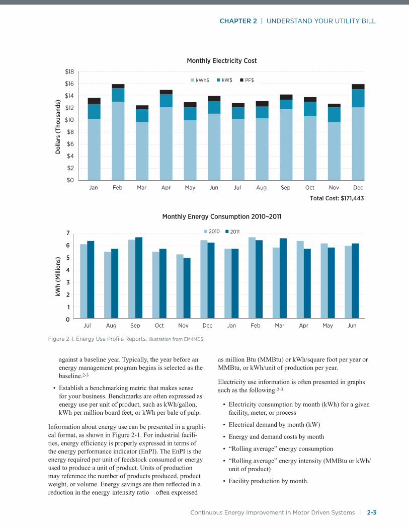
CHAPTER 2 | UNDERSTAND YOUR UTILITY BILL
Continuous Energy Improvement in Motor Driven Systems | 2-3
against a baseline year. Typically, the year before an energy management program begins is selected as the baseline.2-3
• Establish a benchmarking metric that makes sense for your business. Benchmarks are often expressed as energy use per unit of product, such as kWh/gallon, kWh per million board feet, or kWh per bale of pulp.
Information about energy use can be presented in a graphi-cal format, as shown in Figure 2-1. For industrial facili-ties, energy efficiency is properly expressed in terms of the energy performance indicator (EnPI). The EnPI is the energy required per unit of feedstock consumed or energy used to produce a unit of product. Units of production may reference the number of products produced, product weight, or volume. Energy savings are then reflected in a reduction in the energy-intensity ratio—often expressed
as million Btu (MMBtu) or kWh/square foot per year or MMBtu, or kWh/unit of production per year.
Electricity use information is often presented in graphs such as the following:2-3
• Electricity consumption by month (kWh) for a given facility, meter, or process
• Electrical demand by month (kW)
• Energy and demand costs by month
• “Rolling average” energy consumption
• “Rolling average” energy intensity (MMBtu or kWh/unit of product)
• Facility production by month.
Total Cost: $171,443
Monthly Electricity CostD
olla
rs (
Thou
sand
s)
$18
$16
$14
$12
$10
$8
$6
$4
$2
$0Jan Feb Mar Apr May Jun Jul Aug Sep Oct Nov Dec
Monthly Energy Consumption 2010–2011
kWh
(Mill
ions
)
7
6
5
4
3
2
1
0Jul Aug Sep Oct Nov Dec Jan Feb Mar Apr May Jun
kWh$ kW$ PF$
2010 2011
Figure 2-1. Energy Use Profile Reports. Illustration from EM4MDS

CHAPTER 2 | UNDERSTAND YOUR UTILITY BILL
2-4 | Continuous Energy Improvement in Motor Driven Systems
Establish your Facility Baseline Energy UseAn energy baseline is the reference point against which future improvements in plant energy performance must be compared.2-4 A baseline creates a benchmark for compar-ing energy performance from year to year.2-5 The baseline typically encompasses one year’s time period, and can be established at the company, facility, department, or process level.2-4
Energy use over time is often dependent upon one or more independent variables, such as weather, operating
schedule, feedstock variations, or change in product mix. A single or multi-variable regression analysis may be required to track energy use over time.2-4, 2-6 A regression equation allows for an estimate of future energy consump-tion based on changes in these independent variables. This technique provides reliable projections of future energy consumption and is necessary for the subsequent determi-nation of energy savings.2-4
DOE’s EnPI Tool (https://ecenter.ee.doe.gov/EM/tools/Pages/EnPI.aspx) assists industries with their energy baselining and regression analysis efforts.2-7 Access the tool at AMO’s Energy Resource Center (www.eere.energy.gov/manufacturing/tech_assistance/ecenter.html). In addi-tion, the U.S Environmental Protection Agency maintains a database of energy performance indicators for many energy-intensive industries. This database allows you to benchmark your facility against similar production plants by making plant-to-plant energy efficiency comparisons. The EPA database may be accessed at www.energystar.gov/index.cfm?c=in_focus.bus_industries_focus.
Once a baseline energy consumption profile is established, you should break out the total connected horsepower and estimate the quantity of energy used by type of
Helpful Tip
The Plant Energy Profiler (ePEP) software tool is available to help companies profile their energy use and identify potential cost savings. It is available from AMO’s Energy Resource Center (www.eere.energy.gov/manufacturing/tech_assistance/ecenter.html).
Table 2-1. Sawmill Energy End Use Summary.
Process Electricity Use, kWh Percentage of Total Use Cost
Blowers 484,600 4.8% $12,115
Chippers 101,600 1.0% $2,540
Air Compressors 1,911,200 19.0% $47,480
Hog 76,700 0.8% $1,917
Hydraulic Motors 857,800 8.5% $21,445
Saw Motors 2,092,000 20.8% $52,300
Planer Motors 132,700 1.3% $3,317
Kiln Fans 2,033,800 20.2% $50,845
Boiler Fans 268,900 2.7% $6,722
Lights 376,400 3.7% $9,410
Misc. 1,741,390 17.3% $43,534

CHAPTER 2 | UNDERSTAND YOUR UTILITY BILL
Continuous Energy Improvement in Motor Driven Systems | 2-5
plant load (pumps, fans, compressors) or determine the annual energy use for each industrial process. You can then focus your efforts on identifying and analyzing energy efficiency opportunities. You should also verify annual energy and cost savings from installed efficiency measures, examine seasonal loads, consumption trends, and anomalies or unexplained peaks in energy use or demand. Such peaks may indicate equipment malfunction or a meter reading error.2-3 An example of the types of energy end uses at a sawmill is summarized in Table 2-1 and shown in Figure 2-2.
Interpret Utility ChargesA typical electric bill is shown in Figure 2-3. If you look at your own electric bill, it probably tells you how much to pay, but generally does not tell you where the total came from. In contrast, most industrial facility bills include two, three, or more basic charges plus multiple “riders” or energy and demand cost adders.2-1, 2-2 These different charges vary widely from utility to utility. Therefore, your strategies to reduce energy costs depend heavily upon the rate structure applicable to your facility.
Some industries purchase energy from a third-party sup-plier with the local utility only assessing transmission and distribution charges. In this case, the energy manager must obtain monthly billing statements from both the local util-ity and the third-party energy supplier.
While your utility bill indicates how much energy and power you used, the rate structure is your guide for deter-mining how costs are allocated and computed.2-2 Let’s examine the most common charges shown in Figure 2-3, a sample monthly commercial/industrial billing statement. The descriptions below relate to the numbers in Figure 2-3.
1. Service days: The number of days in the billing cycle.
2. Meter number: The number shown on the face of the meter.
3. Meter type: There could be one or more of the following types of meters:
A. Energy consumption and demand: This measures kWh and kW.
B. Reactive energy only: This measures kVARh (kilovolt-amp-hour reactive), which is used to bill for low power factor (generally less than 95%).
C. Energy, demand, and power factor: This meter can measure all three.
4. Meter reading: The actual reading taken from the meter.
5. Multiplier: The multiplier is stamped on the front of the meter and is used in calculating the kW demand, total kWh consumption, or total kVARh consumption.
6. Consumption: The actual meter reading multiplied by the meter multiplier in kWh or kVARh. Reactive power is the nonworking power caused by magnetiz-ing currents required to operate inductive devices such as transformers, motors, and lighting ballasts, and it is used as the basis for power factor charges.
7. Demand: This is the actual kW demand and is cal-culated by multiplying the kW meter reading by the meter multiplier. The demand kW shown is the highest kW recorded by this meter in any 15-minute duration over the monthly billing period.
8. Power factor (PF): The PF percentage shown on the bill is determined from the kVARh consumption described above, along with the real (working) power and apparent (total) power. The actual charge for PF below 95% is calculated by multiplying the kVARh consumption by the kVARh rate.
9. Rate code: This is the rate that applies to the meter number shown. For customers with multiple meters, more than one rate schedule may apply.
10. Unit charge: The rate being charged for the rate code shown. If the rate is not shown, you could have a time-of-use meter. In that case, a second statement is included with your bill that shows the off-peak and on-peak schedule charges.
AirCompressors19%
HydraulicMotors 8%
Saw Motors 21%
Planer Motors 1%
Kiln Fans20% Boiler Fans 3%
Lights 4%
Misc. 17%
Blowers 5%
Chippers 1%
Figure 2-2. Sawmill Energy Consumption Disaggregation.
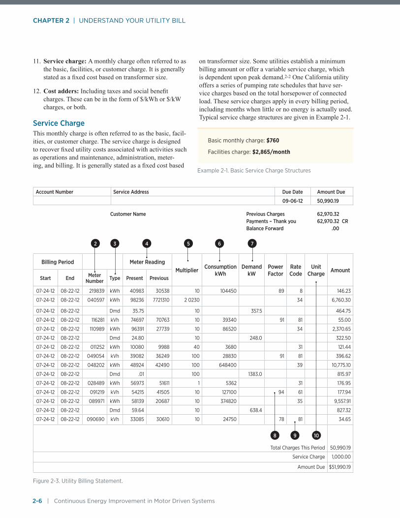
CHAPTER 2 | UNDERSTAND YOUR UTILITY BILL
2-6 | Continuous Energy Improvement in Motor Driven Systems
11. Service charge: A monthly charge often referred to as the basic, facilities, or customer charge. It is generally stated as a fixed cost based on transformer size.
12. Cost adders: Including taxes and social benefit charges. These can be in the form of $/kWh or $/kW charges, or both.
Service ChargeThis monthly charge is often referred to as the basic, facil-ities, or customer charge. The service charge is designed to recover fixed utility costs associated with activities such as operations and maintenance, administration, meter-ing, and billing. It is generally stated as a fixed cost based
on transformer size. Some utilities establish a minimum billing amount or offer a variable service charge, which is dependent upon peak demand.2-2 One California utility offers a series of pumping rate schedules that have ser-vice charges based on the total horsepower of connected load. These service charges apply in every billing period, including months when little or no energy is actually used. Typical service charge structures are given in Example 2-1.
Account Number Service Address Due Date Amount Due
09-06-12 50,990.19
Customer Name Previous Charges 62,970.32 Payments – Thank you 62,970.32 CR Balance Forward .00
Billing Period Meter ReadingMultiplier Consumption
kWhDemand
kWPower Factor
Rate Code
Unit Charge Amount
Start End Meter Number Type Present Previous
07-24-12 08-22-12 219839 kWh 40983 30538 10 104450 89 8 146.23
07-24-12 08-22-12 040597 kWh 98236 7721310 2 0230 34 6,760.30
07-24-12 08-22-12 Dmd 35.75 10 357.5 464.75
07-24-12 08-22-12 116281 kVh 74697 70763 10 39340 91 81 55.00
07-24-12 08-22-12 110989 kWh 96391 27739 10 86520 34 2,370.65
07-24-12 08-22-12 Dmd 24.80 10 248.0 322.50
07-24-12 08-22-12 011252 kWh 10080 9988 40 3680 31 121.44
07-24-12 08-22-12 049054 kVh 39082 36249 100 28830 91 81 396.62
07-24-12 08-22-12 048202 kWh 48924 42490 100 648400 39 10,775.10
07-24-12 08-22-12 Dmd .01 100 1383.0 815.97
07-24-12 08-22-12 028489 kWh 56973 51611 1 5362 31 176.95
07-24-12 08-22-12 091219 kVh 54215 41505 10 127100 94 61 177.94
07-24-12 08-22-12 089971 kWh 58139 20687 10 374820 35 9,557.91
07-24-12 08-22-12 Dmd 59.64 10 638.4 827.32
07-24-12 08-22-12 090690 kVh 33085 30610 10 24750 78 81 34.65
Total Charges This Period 50,990.19
Service Charge 1,000.00
Amount Due $51,990.19
32 4 5 6 7
8 9 10
Figure 2-3. Utility Billing Statement.
Basic monthly charge: $760
Facilities charge: $2,865/month
Example 2-1. Basic Service Charge Structures

CHAPTER 2 | UNDERSTAND YOUR UTILITY BILL
Continuous Energy Improvement in Motor Driven Systems | 2-7
Energy ChargesAll utility rate schedules include an energy charge (some-times called “usage”).2-2 The energy charge is based on the total number of kWh consumed over the billing period. Many utilities offer energy charges that are seasonally differentiated, while some offer rates that vary with the time of day (time of use or TOU schedules). Some utili-ties charge the same rate for all kWh used, while others charge different rates for different quantities or “blocks” of energy. You must use the “tailblock” or marginal energy cost when calculating the cost-effectiveness and feasibility of investments in energy efficiency measures.
With a declining block schedule, the charge per kWh is reduced for each successive block, making the cost per unit less when more electricity is used.2-1 With an “inverted” block structure, the unit price increases for each incremental block. You can consolidate meters to take full advantage of declining block rate schedules. A sample declining block rate structure is shown in Example 2-2.
Demand ChargePeak demand charges can account for more than half of the electric bill in an industrial plant. Demand charges are based on your maximum or peak rate of energy use. The demand charge is similar to a utility “overhead expense” as it is designed to recover costs associated with provid-ing and maintaining enough transmission, switchyard, and distribution infrastructure to meet your peak electrical load.2-8 Demand charges also cover the costs to the utility of building and operating standby electrical generators or peaking plants that must be brought on-line to meet peak loads. Industrial demands can vary greatly, and utility rate schedules are designed so the customers that create peak demands cover the costs to the utility of serving these peak demands.2-9
A typical demand meter averages demand over a specified “demand interval,” usually 15 or 30 minutes. At the end of each interval, the meter resets to zero and the measure-ment begins again.2-2 The meter then stores or records the largest average demand interval in the billing period. Other utilities base their peak demand on the highest “roll-ing average” 15- or 30-minute energy use over the billing
period. These “sliding window” demand meters record demand and then scan for the largest demand interval regardless of starting time.2-2 Short periods of intense use, such as an 8-second motor start-up, have little or no effect on recorded demand. A demand meter is depicted in Fig-ure 2-4.2-3 Utilities are increasingly using digital meters and make billing data available online.
A few utilities base their demand charge on a facility’s instantaneous peak power requirement. In this case, short periods of intense use or motor start-ups after a power out-age can significantly increase demand. You can eliminate demand spikes by sequencing the start-up of large motors so that their individual peak demands are staggered.
Types of Demand Charges
Direct Demand ChargesYou may be billed directly for demand charges at a rate ranging from less than $2/kW per month to more than $25/kW per month, depending on your utility.2-2 In the North-west, both demand and energy charges are higher in the winter months than in the summer months due to the use of electricity for space heating requirements (heat pumps, baseboard heaters, central forced air systems). Winter peak demand charges are rare in the rest of the country as space heating demands are met by natural gas, fuel oil, or wood-fired appliances. In the Atlantic coast, Midwest, South, and Southwest, demand charges peak in the summer because of air-conditioning loads. Utilities often impose season-ally differentiated demand charges or demand cost adders when the facility peak demand occurs during the time of day when the utility load peaks—often during the late afternoon when air conditioning loads are highest.
3.636¢/kWh for the first 40,000 kWh
3.336¢/kWh for all additional kWh
Example 2-2. Declining Block Rate Structure
Helpful Tip
Your plant’s electricity costs may be reduced by revising operating schedules, replacing inefficient equipment, or selecting a different utility rate schedule that better fits your pattern of electricity use.
Ask your electric utility representative for printed rate schedules that describe the various rates available and to illustrate how charges are calculated. Most electric utilities are willing to change a customer’s rate schedule free of charge.2-4 Some utilities require that customers remain on a rate schedule for a contract period of one year.
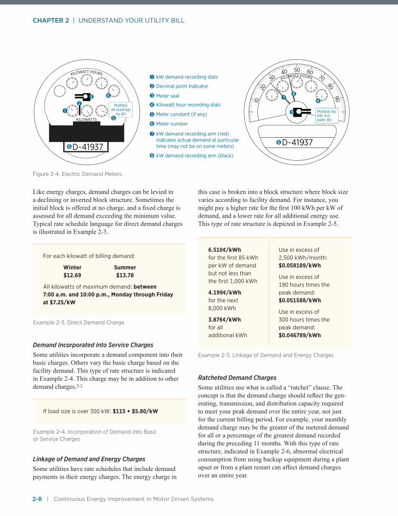
CHAPTER 2 | UNDERSTAND YOUR UTILITY BILL
2-8 | Continuous Energy Improvement in Motor Driven Systems
Like energy charges, demand charges can be levied in a declining or inverted block structure. Sometimes the initial block is offered at no charge, and a fixed charge is assessed for all demand exceeding the minimum value. Typical rate schedule language for direct demand charges is illustrated in Example 2-3.
Demand Incorporated into Service ChargesSome utilities incorporate a demand component into their basic charges. Others vary the basic charge based on the facility demand. This type of rate structure is indicated in Example 2-4. This charge may be in addition to other demand charges.2-2
Linkage of Demand and Energy ChargesSome utilities have rate schedules that include demand payments in their energy charges. The energy charge in
this case is broken into a block structure where block size varies according to facility demand. For instance, you might pay a higher rate for the first 100 kWh per kW of demand, and a lower rate for all additional energy use. This type of rate structure is depicted in Example 2-5.
Ratcheted Demand ChargesSome utilities use what is called a “ratchet” clause. The concept is that the demand charge should reflect the gen-erating, transmission, and distribution capacity required to meet your peak demand over the entire year, not just for the current billing period. For example, your monthly demand charge may be the greater of the metered demand for all or a percentage of the greatest demand recorded during the preceding 11 months. With this type of rate structure, indicated in Example 2-6, abnormal electrical consumption from using backup equipment during a plant upset or from a plant restart can affect demand charges over an entire year.
2 Decimal point indicator
1 kW demand recording dials
4 Kilowatt hour recording dials
Meter constant (if any)5
3 Meter seal
kW demand recording arm (red) indicates actual demand at particular time (may not be on some meters)
7
6 Meter number
kW demand recording arm (black)8
50
D-41937
6070
8090
4030
2010
KILOWATT HOURS
66
78
Multiply by:kW 4.0kWH 80
D-41937
KILOWATT HOURS
KILOWATTS
44
Multiplyall readings
by 801
2
5
3
3
Figure 2-4. Electric Demand Meters.
For each kilowatt of billing demand:
Winter Summer $12.69 $13.78
All kilowatts of maximum demand: between 7:00 a.m. and 10:00 p.m., Monday through Friday at $7.25/kW
Example 2-3. Direct Demand Charge
If load size is over 300 kW: $115 + $5.80/kW
Example 2-4. Incorporation of Demand into Basic or Service Charges
6.510¢/kWh for the first 85 kWh per kW of demand but not less than the first 1,000 kWh
4.199¢/kWh for the next 8,000 kWh
3.876¢/kWh for all additional kWh
Use in excess of 2,500 kWh/month: $0.058189/kWh
Use in excess of 190 hours times the peak demand: $0.051588/kWh
Use in excess of 300 hours times the peak demand: $0.046789/kWh
Example 2-5. Linkage of Demand and Energy Charges
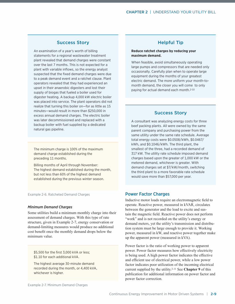
CHAPTER 2 | UNDERSTAND YOUR UTILITY BILL
Continuous Energy Improvement in Motor Driven Systems | 2-9
Minimum Demand ChargesSome utilities build a minimum monthly charge into their assessment of demand charges. With this type of rate structure, given in Example 2-7, energy conservation or demand-limiting measures would produce no additional cost benefit once the monthly demand drops below the minimum value.
Power Factor ChargesInductive motor loads require an electromagnetic field to operate. Reactive power, measured in kVAR, circulates between the generator and the load to excite and sus-tain the magnetic field. Reactive power does not perform “work” and is not recorded on the utility’s energy or demand meters, yet the utility’s transmission and distribu-tion system must be large enough to provide it. Working power, measured in kW, and reactive power together make up the apparent power (measured in kVA).
Power factor is the ratio of working power to apparent power. Power factor measures how effectively electricity is being used. A high power factor indicates the effective and efficient use of electrical power, while a low power factor indicates poor utilization of the incoming electrical current supplied by the utility.2-11 See Chapter 9 of this publication for additional information on power factor and power factor correction.
Success Story
An examination of a year’s worth of billing statements for a regional wastewater treatment plant revealed that demand charges were constant over the last 7 months. This is not expected for a plant with variable inflows, so the energy analyst suspected that the fixed demand charges were due to a peak demand event and a ratchet clause. Plant operators revealed that they had experienced an upset in their anaerobic digesters and lost their supply of biogas that fueled a boiler used for digester heating. A backup 4,000 kW electric boiler was placed into service. The plant operators did not realize that turning this boiler on—for as little as 15 minutes—would result in more than $250,000 in excess annual demand charges. The electric boiler was later decommissioned and replaced with a backup boiler with fuel supplied by a dedicated natural gas pipeline.
Helpful Tip
Reduce ratchet charges by reducing your maximum demand.
When feasible, avoid simultaneously operating large pumps and compressors that are needed only occasionally. Carefully plan when to operate large equipment during the months of your greatest electric demand. The more uniform your month-to-month demand, the closer you will come to only paying for actual demand each month.2-10
Success Story
A consultant was analyzing energy costs for three beef packing plants. All were owned by the same parent company and purchasing power from the same utility under the same rate schedule. Average total energy costs were $0.0508/kWh, $0.0467/kWh, and $0.1046/kWh. The third plant, the smallest of the three, had a recorded demand of 317 kW. The utility rate schedule imposed demand charges based upon the greater of 1,000 kW or the metered demand, whichever is greater. With demand charges set at $7/kW/month, switching the third plant to a more favorable rate schedule would save more than $57,000 per year.
The minimum charge is 100% of the maximum demand charge established during the preceding 11 months.
Billing months of April through November: The highest demand established during the month, but not less than 60% of the highest demand established during the previous winter season.
Example 2-6. Ratcheted Demand Charges
$5,500 for the first 3,000 kVA or less; $1.10 for each additional kVA.
The highest average 30-minute demand recorded during the month, or 4,400 kVA, whichever is higher.
Example 2-7. Minimum Demand Charges

CHAPTER 2 | UNDERSTAND YOUR UTILITY BILL
2-10 | Continuous Energy Improvement in Motor Driven Systems
Utilities often assess a penalty for low power factor on their commercial and industrial rate schedules. Various methods exist for calculating the penalty. Understanding your utility’s calculation method enables you to deter-mine the benefits associated with potential power factor improvements.
Types of Power Factor Penalties
kVA BillingAs shown in Example 2-8, the utility may measure and bill for every kilovolt-amp of apparent power or primary period (peak) kVA supplied, including reactive current.
Direct Reactive Energy ChargesAs indicated in Example 2-9, reactive power may be mea-sured and a reactive energy charge levied (in ¢/kVARh).
Demand Billing with a Power Factor AdjustmentIn the following calculation, the utility bills the customer at normal demand rates with a demand surcharge or multi-plier included to account for low power factor.
Given a facility power factor of 84%, the utility would obtain a 13% increase in billable demand (95/84) = 1.13. With this form of low power factor penalty, a facility with a metered demand of 1,000 kW would have a bill-able demand of 1,130 kW. At $10/kW/month, the pen-alty due to low power factor is 130 kW × $10/kW/month × 12 months/year = $15,600 annually. This low power factor penalty can be eliminated through the installation of capacitors at individual motors or at the plant service entrance.
Example 2-10 shows an example of a rate schedule with a penalty for facilities operating below a power factor of 95%.
Excess kVAR Reactive Demand ChargesWith this low power factor penalty method, the utility imposes a direct charge for the use of magnetizing power in excess of some percentage of kW demand. For example, if the charge was $0.60/kVAR for everything over 40% of kW, and the peak load was 4,000 kW, then the utility would provide up to 1,600 kVAR at no cost. Excess kVAR is billable at the specified rate. This type of rate structure is illustrated in Example 2-11.
Demand charge: $2.49/kVA of billing demand
Primary kVA charge: $24,000, which includes 2,000 primary kVA plus $12.10 for each additional primary kVA.
Example 2-8. kVA Billing
The maximum 15-minute reactive demand for the month in kVAR in excess of 40% of the kilowatt demand for the same month will be billed at $0.45/kVAR of such excess reactive demand.
Example 2-11. Excess kVAR Reactive Demand Charges
The demand charge, before adjustment for power factor, will be increased 1% for each 1% by which the average power factor is less than 0.95 lagging.
The demand charge increases by 1% for each 1% the power factor is less than 85% and decreases by 1% for each percent the power factor is above 90%.
Example 2-10. Demand Billing with a Power Factor Adjustment
kWBILLED = kWDEMAND × 0.95
PF
kWBILLED = Adjusted or billable demand
kWDEMAND = Measured electric demand, in kW
PF = Power factor, as a decimal
Equation 2-1
Reactive power charge: 0.061¢/kVARh
Example 2-9. Direct Reactive Energy Charges

CHAPTER 2 | UNDERSTAND YOUR UTILITY BILL
Continuous Energy Improvement in Motor Driven Systems | 2-11
Optional Rate Schedules
Time-of-Use RatesBy charging more during the peak period, when incremen-tal costs are highest, time-of-use utility rates send accurate marginal-cost price signals to customers. Periods of heavy electricity use are typically defined as “peak” hours; peri-ods of lower use are “shoulder” hours, and times of lowest use are deemed “off-peak.” Energy charges between peak and off-peak times might vary by more than $0.10/kWh.
Similarly, your demand charges may be computed at a much higher rate if your highest-demand interval occurs during the peak hours.2-10
Interruptible, Curtailment, and Customer Generator RatesAt the electric utility’s request, customers on interruptible rates must lower their demand. They can do this by turn-ing off some or all of their large electrically driven equip-ment, or they can use emergency generators or engine-driven pumps instead of utility-supplied power.2-10
To obtain interruptible, curtailment, or customer generator rates, the customer enters into a load management agree-ment to interrupt or reduce plant loads at the request of the power company during the occasional times of peak demand. In return, the power company applies lower rates to the demand charge on the bill for the duration of the agreement. Penalties for nonconformance, however, are high.2-10
Use Billing Data to Identify Savings OpportunitiesUnderstanding your electric utility bill—knowing how your demand meter works and how power factor penalties are assessed—is crucial. Energy and demand costs are controllable, and the benefits of implementing energy conservation, demand management, or power fac-tor correction are directly related to the way your facility operates and the structure of your rate schedule. While power factor correction is not generally undertaken for energy conservation reasons, it can result in a reduction in electrical resistance (I2R) losses within the plant distribution system; it can be very cost-effective and therefore can result in significant reductions in your utility bills.
For a specific utility rate schedule, it is useful to quantify the energy charges and demand charges for a constant 100-kW load operating for a single shift, two shifts, and three shifts, or continuous operation.
Many efficiency measures reduce peak demand and result in energy use reductions. Avoid basing cost savings on “average” energy costs that are based on total monthly or annual utility costs divided by total electrical energy use. Always determine the expected demand reduction and energy savings for an efficiency measure, and then determine cost savings by multiplying the reductions by the appropriate demand and marginal or incremental energy charges.
Another way you can assess the feasibility of demand management measures is by computing your facility load factor. Contact your utility account representative to determine if the utility can provide load data by hour or 15-minute intervals. Often, energy data can be down-loaded from “smart” meters. (A smart meter is an elec-trical meter that records consumption of electric energy in intervals of an hour or less and that provides remote reporting to a Web portal. The portal is often accessible by the facility operator’s personal computer (PC), iPhone, iPod, or Android application.
Helpful Tip
If you are on a time-of-use rate, you should consider shifting as many operations to the off-peak period as possible, along with other demand control measures. Significant investments in added equipment may be justified by savings in energy and demand charges.
If your facility is not on a time-of-use rate, find out whether your electric utility offers such rates. You may be able to reduce costs by switching to time-of-use rates.
Helpful Tip
Find out whether your electric utility offers interruptible, curtailment, or customer generator rates. If you are considering using an emergency generator on a regular basis, analyze operating conditions as well as your ability to maintain the generator. Talk with your utility account representative about a load management agreement.

CHAPTER 2 | UNDERSTAND YOUR UTILITY BILL
2-12 | Continuous Energy Improvement in Motor Driven Systems
Load factor (LF) is the ratio of your facility’s average to peak demand and indicates how effectively demand is allocated. A low load factor indicates a possible potential for demand reduction through load scheduling that results in “clipping peaks” and “filling valleys.” Calculate your monthly load factor for a 12-month period so monthly minimum, maximum, and an annual average load factor can be determined.2-12 A sample load factor calculation is given in Example 2-14.
If your load factor varies significantly from billing period to billing period, you should carefully review your opera-tion. Many software tools and/or commercial services are available to assist a company in analyzing their energy use patterns. Opportunities for in-plant demand reduction measures likely exist when an annual load factor is less than 80%. In contrast, if your facility has a load factor that is constantly above 80%, there is probably little potential for demand-limiting measures.2-12
If your facilities have low load factors, you must deter-mine the load profile—or load variation by time of day or month—for major processes or pieces of equipment within the plant. Compile load data by conducting periodic data logging equipment.
Figure 2-5. Utility Rate Schedule with High Demand Charges
Utility 1
Large General Service (1,000 kW to 10,000 kW)
Demand Charge = $13.43/kW/month (Average Annual)
Avg On-peak Energy Charge = $0.01792/kWh (7 a.m. – 8 p.m.)
Avg Off-peak Energy Charge = $0.00902/kWh
Single Shift
Two Shifts
Three Shifts
Total Demand Cost $16,116 $16,116 $16,116
Total Energy Cost $3,582 $6,275 $10,466
Demand Charges % 81.8% 72% 60.6%
The rate schedule for Utility 1 (shown in Figure 2-5) is characterized by a high demand charge and low energy charges—particularly for off-peak energy. Demand-related charges account for more than 81% of total utility costs for an industrial plant operating a single shift in this utility’s service territory. Energy charges account for only 19% of a typical utility bill. This brief analysis indicates that consideration of demand management measures, such as load limiting controls, energy storage, or chiller cycling could provide significant benefits at this site. Efficiency measures such as light-emitting diode (LED) parking lot and security lighting would provide energy savings, but minimal cost savings for plants purchasing energy under this rate schedule.
Example 2-12. Breakout of Operating Costs for Utility with High Demand Charges
In contrast, demand charges account for less than 50% of total utility costs for a plant running a single shift and purchasing energy and power under Utility 2’s rate schedule (see Figure 2-6). Given a three-shift operation, demand charges account for only 18% of total utility costs. In this instance, investing in efficiency measures that save energy would provide significant utility cost reductions.
Example 2-13. Breakout of Operating Costs for Utility with Moderate Demand Charges
Figure 2-6. Utility Rate Schedule with Moderate Demand Charges
Utility 2
Large General Service
Demand Charge = $7.71/kW/month (June–Sept.), $6.30/kW/month
Energy Charge = $0.04225/kWh
Single Shift
Two Shifts
Three Shifts
Total Demand Cost $8,124 $8,124 $8,124
Total Energy Cost $8,788 $17,576 $37,011
Demand Charges % 48.0% 31.6% 18.0%
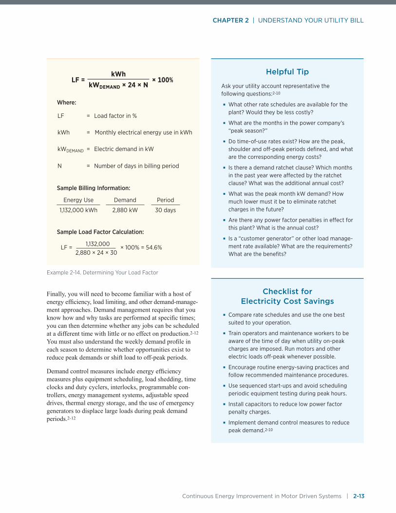
CHAPTER 2 | UNDERSTAND YOUR UTILITY BILL
Continuous Energy Improvement in Motor Driven Systems | 2-13
Finally, you will need to become familiar with a host of energy efficiency, load limiting, and other demand-manage-ment approaches. Demand management requires that you know how and why tasks are performed at specific times; you can then determine whether any jobs can be scheduled at a different time with little or no effect on production.2-12 You must also understand the weekly demand profile in each season to determine whether opportunities exist to reduce peak demands or shift load to off-peak periods.
Demand control measures include energy efficiency measures plus equipment scheduling, load shedding, time clocks and duty cyclers, interlocks, programmable con-trollers, energy management systems, adjustable speed drives, thermal energy storage, and the use of emergency generators to displace large loads during peak demand periods.2-12
Helpful Tip
Ask your utility account representative the following questions:2-10
■■ What other rate schedules are available for the plant? Would they be less costly?
■■ What are the months in the power company’s “peak season?”
■■ Do time-of-use rates exist? How are the peak, shoulder and off-peak periods defined, and what are the corresponding energy costs?
■■ Is there a demand ratchet clause? Which months in the past year were affected by the ratchet clause? What was the additional annual cost?
■■ What was the peak month kW demand? How much lower must it be to eliminate ratchet charges in the future?
■■ Are there any power factor penalties in effect for this plant? What is the annual cost?
■■ Is a “customer generator” or other load manage-ment rate available? What are the requirements? What are the benefits?
LF = kWh
× 100%kWDEMAND × 24 × N
Where:
LF = Load factor in %
kWh = Monthly electrical energy use in kWh
kWDEMAND = Electric demand in kW
N = Number of days in billing period
Sample Billing Information:
Energy Use Demand Period
1,132,000 kWh 2,880 kW 30 days
Sample Load Factor Calculation:
1,132,000 LF = 2,880 × 24 × 30
× 100% = 54.6%
Example 2-14. Determining Your Load Factor
Checklist for Electricity Cost Savings
■■ Compare rate schedules and use the one best suited to your operation.
■■ Train operators and maintenance workers to be aware of the time of day when utility on-peak charges are imposed. Run motors and other electric loads off-peak whenever possible.
■■ Encourage routine energy-saving practices and follow recommended maintenance procedures.
■■ Use sequenced start-ups and avoid scheduling periodic equipment testing during peak hours.
■■ Install capacitors to reduce low power factor penalty charges.
■■ Implement demand control measures to reduce peak demand.2-10

CHAPTER 2 | UNDERSTAND YOUR UTILITY BILL
2-14 | Continuous Energy Improvement in Motor Driven Systems
References 2-1 A & C Consultants, Inc., Managing Energy in Local
Government Facilities, Washington State Energy Office, WAOENG-866686-07, March 1987.
2-2 Washington Energy Extension Service, Under-standing Commercial Electric Bills, January 1986.
2-3 Bonneville Power Administration, “Energy Accounting,” Electric Ideas Clearinghouse Technology Update, November 1991.
2-4 U.S. Department of Energy, eGuide for ISO 50001, available from the AMO Energy Resource Center at ecenter.ee.doe.gov/EM/SPM/Pages/Home.aspx.
2-5 U.S. Department of Energy, Steps to Develop a Baseline: A Guide to Developing an Energy Use and Energy Intensity Baseline and the Reporting Requirements for the Save Energy Now Leader Pledge, October 2008.
2-6 Northwest Energy Efficiency Alliance, Field Guide, April 2012.
2-7 U.S. Department of Energy, EnPI Tool Instruction Guide, February 2011.
2-8 National Grid, Understanding Electric Demand: For National Grid’s Commercial Customers in New York, NY0620, December 2005.
2-9 Wisconsin Focus on Energy, Understanding Your Electric Bill, Technical Data Sheet, BP-1828-0207, 2007.
2-10 Electric Power Research Institute, Understand-ing Your Electric Bill: Cost-Saving Strategies for Industrial and Large Electric Power Consumers, BR-104028, 1994.
2-11 Eaton Electrical, Power Factor Correction: A Guide for the Plant Engineer, November 2010.
2-12 Bonneville Power Administration, “Electrical Demand Control for Industry,” Electric Ideas Clearinghouse Technology Update, February 1993.

CHAPTER 3 CONDUCTING A MOTOR SURVEY

CHAPTER 3 | CONDUCTING A MOTOR SURVEY
3-2 | Continuous Energy Improvement in Motor Driven Systems
Conducting a field evaluation of motors is essential in mak-ing informed decisions regarding motor selection and use. The amount of money you can save by purchasing a pre-mium efficiency motor instead of an energy-efficient motor depends on the horsepower rating of the motor, annual hours of use, load factor, efficiency gain (at the load point), and the serving utility’s charges for electrical energy and demand.3-1 Field measurements are necessary to establish the load imposed on an existing motor by its driven equip-ment and to determine motor efficiency at its load point.
Motor Survey Techniques and Information RequirementsIt is impossible to manage something when you do not know what you have.3-1 Experience shows that facility personnel usually underestimate the number of motors in operation at their plant. When motors are actually counted, the actual number of motors can be two-to-three times the original presumption.3-1, 3-2
The first step in a motor management program is to pre-pare a strategy for obtaining nameplate, application, and operating data for both operating and spare motors. Has your plant electrician or maintenance manager compiled an electronic motors database or does he or she maintain an inventory management system?
Many large organizations use CMMS software that con-tains an equipment list. At many facilities, even when an electronic motor database is available, it is often inaccu-rate, incomplete, outdated, or otherwise not well-main-tained. Medium and small industrial facilities sometimes rely on a card file for record-keeping while a surprising number of facilities have no information on their motor population whatsoever. Do not be surprised if the needed information for each motor is missing or incomplete. Often, only the motor identification number (motor ID), location, horsepower rating, synchronous speed, and full-load current values are recorded and available.
Companies that operate predictive maintenance programs or that employ condition assessment techniques often use a motor analyzer that contains an internal motor database plus a field measurements database that allows for the “health” of individual motors to be monitored and trended. Condition assessment activities often focus on only a sub-set of a plant’s motor population, i.e., on critical motors, larger motors, or motors that are thought to be approach-ing end of life or where an impending failure is thought to be imminent. Use of common equipment identification
numbers allows the condition assessment program’s field measurements library to be merged into the broader motor inventory database.
Even when an electronic motors database is available, it is not unusual for the motor’s full-load efficiency value to be missing. As one plant electrician stated, “That informa-tion is just not useful for me.” Motor full-load efficiency values are critical inputs for a motor energy management team as they indicate the efficiency class (standard, energy efficient, premium efficiency) of the motor.
Sometimes, a motor inventory includes only in-service or operating motors. In these instances, nameplate infor-mation for spare motors must be obtained. Other times, equipment lists or motor inventories include entries for motors, driven equipment, and process lines that have been taken out of service, are obsolete, or are inoperable.
The assignment of equipment numbers is often chrono-logical. Motors are assigned progressively higher num-bers when they are purchased, for example, MO-001…to MO-867. When purchase or installation dates are also available, the motor identification number can then be used to quickly identify the pre-1997 motors that are likely to be of older, standard efficiency designs. Some motor manufacturers stamp the date that the motor was manufac-tured onto the motor nameplate.
Gathering nameplate information and taking field mea-surements can be a daunting task as a large industrial facility may have several thousand operating motors plus hundreds of spares.3-3 While maintenance staff might desire complete information on ALL motors in the plant—for maintenance logging and inventory management purposes—the energy management team may reduce its workload by applying filtering criteria so it focuses on the motors that cost the most to maintain and operate. These are the motors that are large, heavily loaded, run long hours, and are in poor condition.3-4
When initiating a motor survey, first consider the single-speed, three-phase, low voltage AC induction motors in a plant that are rated between 20 to 500 horsepower. These motors are covered by the premium full-load efficiency standards. On the initial survey, do not include single-phase, hermetically sealed, submersible pump, DC or synchronous motors, NEMA Design C and D motors, centrifuge, crane/hoist, or punch press motors, motors with synchronous speeds of 720 RPM or lower, motors already controlled by an adjustable speed drive, motors that operate with intermittent, cyclic, or fluctuating load-ing, or motors designed to operate above 600 V (medium
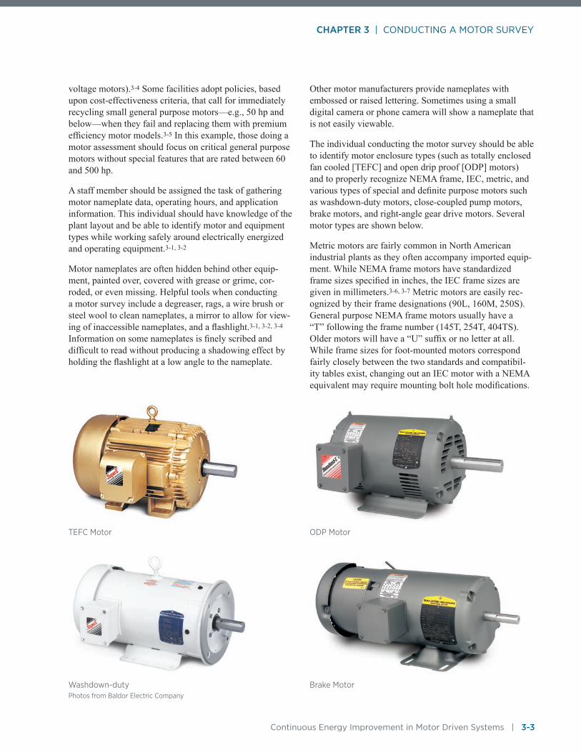
CHAPTER 3 | CONDUCTING A MOTOR SURVEY
Continuous Energy Improvement in Motor Driven Systems | 3-3
voltage motors).3-4 Some facilities adopt policies, based upon cost-effectiveness criteria, that call for immediately recycling small general purpose motors—e.g., 50 hp and below—when they fail and replacing them with premium efficiency motor models.3-5 In this example, those doing a motor assessment should focus on critical general purpose motors without special features that are rated between 60 and 500 hp.
A staff member should be assigned the task of gathering motor nameplate data, operating hours, and application information. This individual should have knowledge of the plant layout and be able to identify motor and equipment types while working safely around electrically energized and operating equipment.3-1, 3-2
Motor nameplates are often hidden behind other equip-ment, painted over, covered with grease or grime, cor-roded, or even missing. Helpful tools when conducting a motor survey include a degreaser, rags, a wire brush or steel wool to clean nameplates, a mirror to allow for view-ing of inaccessible nameplates, and a flashlight.3-1, 3-2, 3-4 Information on some nameplates is finely scribed and difficult to read without producing a shadowing effect by holding the flashlight at a low angle to the nameplate.
Other motor manufacturers provide nameplates with embossed or raised lettering. Sometimes using a small digital camera or phone camera will show a nameplate that is not easily viewable.
The individual conducting the motor survey should be able to identify motor enclosure types (such as totally enclosed fan cooled [TEFC] and open drip proof [ODP] motors) and to properly recognize NEMA frame, IEC, metric, and various types of special and definite purpose motors such as washdown-duty motors, close-coupled pump motors, brake motors, and right-angle gear drive motors. Several motor types are shown below.
Metric motors are fairly common in North American industrial plants as they often accompany imported equip-ment. While NEMA frame motors have standardized frame sizes specified in inches, the IEC frame sizes are given in millimeters.3-6, 3-7 Metric motors are easily rec-ognized by their frame designations (90L, 160M, 250S). General purpose NEMA frame motors usually have a “T” following the frame number (145T, 254T, 404TS). Older motors will have a “U” suffix or no letter at all. While frame sizes for foot-mounted motors correspond fairly closely between the two standards and compatibil-ity tables exist, changing out an IEC motor with a NEMA equivalent may require mounting bolt hole modifications.
TEFC Motor
Washdown-duty Photos from Baldor Electric Company
Brake Motor
ODP Motor
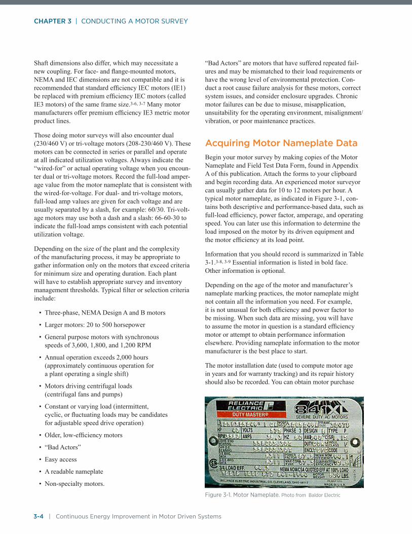
CHAPTER 3 | CONDUCTING A MOTOR SURVEY
3-4 | Continuous Energy Improvement in Motor Driven Systems
Shaft dimensions also differ, which may necessitate a new coupling. For face- and flange-mounted motors, NEMA and IEC dimensions are not compatible and it is recommended that standard efficiency IEC motors (IE1) be replaced with premium efficiency IEC motors (called IE3 motors) of the same frame size.3-6, 3-7 Many motor manufacturers offer premium efficiency IE3 metric motor product lines.
Those doing motor surveys will also encounter dual (230/460 V) or tri-voltage motors (208-230/460 V). These motors can be connected in series or parallel and operate at all indicated utilization voltages. Always indicate the “wired-for” or actual operating voltage when you encoun-ter dual or tri-voltage motors. Record the full-load amper-age value from the motor nameplate that is consistent with the wired-for-voltage. For dual- and tri-voltage motors, full-load amp values are given for each voltage and are usually separated by a slash, for example: 60/30. Tri-volt-age motors may use both a dash and a slash: 66-60-30 to indicate the full-load amps consistent with each potential utilization voltage.
Depending on the size of the plant and the complexity of the manufacturing process, it may be appropriate to gather information only on the motors that exceed criteria for minimum size and operating duration. Each plant will have to establish appropriate survey and inventory management thresholds. Typical filter or selection criteria include:
• Three-phase, NEMA Design A and B motors
• Larger motors: 20 to 500 horsepower
• General purpose motors with synchronous speeds of 3,600, 1,800, and 1,200 RPM
• Annual operation exceeds 2,000 hours (approximately continuous operation for a plant operating a single shift)
• Motors driving centrifugal loads (centrifugal fans and pumps)
• Constant or varying load (intermittent, cyclic, or fluctuating loads may be candidates for adjustable speed drive operation)
• Older, low-efficiency motors
• “Bad Actors”
• Easy access
• A readable nameplate
• Non-specialty motors.
“Bad Actors” are motors that have suffered repeated fail-ures and may be mismatched to their load requirements or have the wrong level of environmental protection. Con-duct a root cause failure analysis for these motors, correct system issues, and consider enclosure upgrades. Chronic motor failures can be due to misuse, misapplication, unsuitability for the operating environment, misalignment/vibration, or poor maintenance practices.
Acquiring Motor Nameplate Data Begin your motor survey by making copies of the Motor Nameplate and Field Test Data Form, found in Appendix A of this publication. Attach the forms to your clipboard and begin recording data. An experienced motor surveyor can usually gather data for 10 to 12 motors per hour. A typical motor nameplate, as indicated in Figure 3-1, con-tains both descriptive and performance-based data, such as full-load efficiency, power factor, amperage, and operating speed. You can later use this information to determine the load imposed on the motor by its driven equipment and the motor efficiency at its load point.
Information that you should record is summarized in Table 3-1.3-8, 3-9 Essential information is listed in bold face. Other information is optional.
Depending on the age of the motor and manufacturer’s nameplate marking practices, the motor nameplate might not contain all the information you need. For example, it is not unusual for both efficiency and power factor to be missing. When such data are missing, you will have to assume the motor in question is a standard efficiency motor or attempt to obtain performance information elsewhere. Providing nameplate information to the motor manufacturer is the best place to start.
The motor installation date (used to compute motor age in years and for warranty tracking) and its repair history should also be recorded. You can obtain motor purchase
Figure 3-1. Motor Nameplate. Photo from Baldor Electric
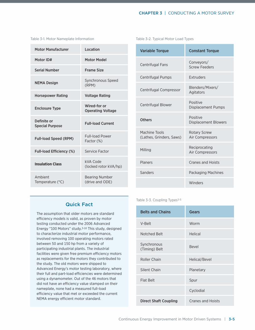
CHAPTER 3 | CONDUCTING A MOTOR SURVEY
Continuous Energy Improvement in Motor Driven Systems | 3-5
Quick Fact
The assumption that older motors are standard efficiency models is valid, as proven by motor testing conducted under the 2006 Advanced Energy “100 Motors” study.3-10 This study, designed to characterize industrial motor performance, involved removing 100 operating motors rated between 50 and 150 hp from a variety of participating industrial plants. The industrial facilities were given free premium efficiency motors as replacements for the motors they contributed to the study. The old motors were shipped to Advanced Energy’s motor testing laboratory, where their full and part-load efficiencies were determined using a dynamometer. Out of the 46 motors that did not have an efficiency value stamped on their nameplate, none had a measured full-load efficiency value that met or exceeded the current NEMA energy efficient motor standard.
Table 3-1. Motor Nameplate Information
Motor Manufacturer Location
Motor ID# Motor Model
Serial Number Frame Size
NEMA Design Synchronous Speed (RPM)
Horsepower Rating Voltage Rating
Enclosure Type Wired-for or Operating Voltage
Definite or Special Purpose Full-load Current
Full-load Speed (RPM) Full-load Power Factor (%)
Full-load Efficiency (%) Service Factor
Insulation Class kVA Code (locked rotor kVA/hp)
Ambient Temperature (°C)
Bearing Number (drive and ODE)
Table 3-2. Typical Motor Load Types
Variable Torque Constant Torque
Centrifugal FansConveyors/ Screw Feeders
Centrifugal Pumps Extruders
Centrifugal CompressorBlenders/Mixers/ Agitators
Centrifugal BlowerPositive Displacement Pumps
Others Positive Displacement Blowers
Machine Tools (Lathes, Grinders, Saws)
Rotary Screw Air Compressors
MillingReciprocating Air Compressors
Planers Cranes and Hoists
Sanders Packaging Machines
Winders
Table 3-3. Coupling Types3-5
Belts and Chains Gears
V-Belt Worm
Notched Belt Helical
Synchronous (Timing) Belt
Bevel
Roller Chain Helical/Bevel
Silent Chain Planetary
Flat Belt Spur
Cyclodial
Direct Shaft Coupling Cranes and Hoists

CHAPTER 3 | CONDUCTING A MOTOR SURVEY
3-6 | Continuous Energy Improvement in Motor Driven Systems
and installation dates and repair histories from maintenance histories from maintenance records, work orders, or from people who have worked at the plant and can recall motor histories. Once motor data have been gathered, a “motor tree” can be used to provide a snapshot of the in-service and spare motor population in the plant (see Figure 3-2.)
Obtaining Application InformationUse the “Motor Nameplate and Field Test Data Form” contained in Appendix A when conducting your motor survey. Describe the motor load (the device being driven), identify the coupling type, indicate whether load modula-tion devices such as throttling valves or inlet guide vanes are in use, and record the driven-equipment speed. This information should prove useful in future energy man-agement efforts, such as replacing V-belts with synchro-nous or notched belts or when considering adjustable speed drives for centrifugal equipment with variable flow requirements. See Tables 3-1 and 3-2 for lists of load and coupling types.
The nature of the load being served by the motor is also important. Motors coupled to variable-speed drives, oper-ating with low load factors, or those that serve intermit-tent, cyclic, or randomly acting loads may not be cost-effective candidates for an efficiency upgrade.
Annual Operating Hour AssumptionsAn estimation of annual operating hours and motor load is needed to determine energy and cost savings from any motor efficiency improvement measure. These are critical pieces of information, as energy savings vary directly with assumptions regarding motor load and annual operating hours. At the same time, an evaluation has shown that customer-provided estimates of operating hours can devi-ate significantly from actual operating hours. One electric utility provided a rebate for the purchase and operation of high efficiency electric motors in commercial and indus-trial settings. The rebates were awarded at the time of pur-chase based on customer-supplied operating hour values. To verify to utility regulators that the predicted energy sav-ings were realized, the utility performed field monitoring
DC Motors5 units24.5 hp
Large hp>=500 hp
2 units
U-Frame Motors70 units1,786 hp
DC Motors12 units295 hp
Large hp> 500 hp9 units
7,100 hp
Old U-Frame Motors31 units1,035 hp
Critical Motor Inventory
In-Service Motors3 to 800 hp
175 units - 13,662 hp
Spare Motors229 units - 7,966 hp
Low Voltage<600 Volts
163 units5,612 hp
Medium Voltage4,000 Volts
12 units8,050 hp
Low Voltage<600 Volts230 units5,093 hp
Medium Voltage4,000 Volts
2 units3,100 hp
Plant Annual Energy Use, 2010–2011
50.4 million kWh
Figure 3-2. A “Motor Tree” for In-Service and Spare Motors

CHAPTER 3 | CONDUCTING A MOTOR SURVEY
Continuous Energy Improvement in Motor Driven Systems | 3-7
of a subset of the installed high efficiency motors.3-12 TOU data loggers were installed to record motor start and stop times by sensing the magnetic field created when the motor is operating. Loggers were left on 59 motors (83% were industrial applications) for an average of about 1,600 hours (9.5 weeks). The study found considerable variance between the customer-reported and measured annual oper-ating hour values, and concluded that “customers have a difficult time accurately estimating annual motor run time” and “customers may not be able to accurately estimate operating hours for individual motors.” 3-12
The wide variation between customer-reported and mea-sured motor operating hour values is shown in Figure 3-3. The vertical axis indicates measured operating hour values with the horizontal axis giving customer-reported hours. With this type of plot, good agreement is evident when the value falls on the 45º line. The plot shows that good agreement was rarely achieved. Measured or “true” values ranged from 0 to 8,000 hours per year for a customer-assumed value of 2,000 hours; and from 500 to 8,760 hours for estimates of 6,500 hours.
Assumptions regarding annual motor operating hours can be improved through talking directly with the plant engineer and plant operations staff. Ask how many hours a motor is used on each shift. In food processing plants, the third shift might involve sanitization activities with a different group of motors being heavily utilized. Does the motor operation change on weekends? Is a backup pump
or redundant process train available for a particular appli-cation? For instance, a boiler might have two feedwater pumps, with the units rotated each week to equalize wear. This type of operation must be reflected in motor operat-ing hour estimates.
Estimating Motor LoadVarious studies have shown that motors are often loaded to between 65% and 75% of their rated output. In this load range, motors often operate at an efficiency that is greater than their full-load efficiency. In addition to monitor-ing operating hours, the PGE study involved taking field measurements at 39 operating motors. On average, the 39 motors were found to be operating at 74% of their rated horsepower. Field measurements taken of 324 motors at a naval shipyard showed an average load of 67.6%.3-13 Mea-surements taken for 102 motors at a pulp mill indicated an average load of 70.1%.3-14
To estimate the actual load imposed upon the motor by its driven equipment, it is necessary to measure all of the following at each motor:
• Power, in kW, or
• Line-to-line voltage between all three phases, and
- Current values for all three phases, or
- Operating speed of the motor and driven equipment.
The equipment necessary for these measurements includes:
• Voltmeter, multimeter, or power meter
• Clamp-on ammeter
• Power factor meter
• Tachometer.
Meters should be of adequate quality to read true root mean square (RMS) values. This guidebook assumes that the electrician uses meters of adequate accuracy.
Methods of determining motor load from field measure-ments are given in Chapter 5. When the motor operates at a constant load, only one set of measurements is necessary. When the motor drives a variable load or operates at two or three distinct load points, data logging of input power or current over time is required. The electrician can then determine the weighted average motor load or develop a load profile that shows the percentage of operating hours at each load point (for additional information on load profiles see Chapter 8).Figure 3-3. Operating Hour Assumptions Versus
Measured Values3-12
Original Program Estimated Hours
Hou
rs B
ased
on
Met
ered
Dat
a
0
4,000
4,0
00
3,000
3,0
00
2,000
2,0
00
1,000
1,00
0
5,000
5,0
00
6,000
6,0
00
7,000
7,0
00
8,000
8,0
00
9,000
9,0
00
Ideal: Measured = Estimated

CHAPTER 3 | CONDUCTING A MOTOR SURVEY
3-8 | Continuous Energy Improvement in Motor Driven Systems
Motor and driven-equipment speeds must be measured as closely as possible, ideally with a strobe tachometer. Motor speed is important, because a replacement motor should duplicate the existing motor speed. When driving centrifu-gal loads (fans and pumps), the motor load is highly sensi-tive to operating speed. A premium efficiency motor usually operates at a slightly higher speed than a standard effi-ciency motor. The higher speed may result in an increase in speed-sensitive loads; this can negate savings resulting from improving motor efficiency. A speed/load correction is necessary to properly evaluate savings from a premium effi-cient motor energy efficiency opportunity.3-15, 3-16
Once you have collected nameplate, annual operating hours, and operating data for each motor in your filtered or short list of motors, you can enter this information into DOE’s MotorMaster+ software tool. MotorMaster+ allows users to create an in-plant motor inventory database with a record for each motor. When utility cost data and field measurements are available, the software tool automati-cally calculates the annual energy use and costs for each motor. When field measurements are entered (see the “Taking Field Measurements” section of this chapter), the software tool determines the load on the motor, average operating voltage, and voltage unbalance. MotorMaster+ load and efficiency estimation algorithms are discussed in the tool users guide and in Chapter 5.3-17 MotorMaster+ motor management capabilities are discussed in detail in Chapter 7.
MotorMaster+ also provides a Motor Efficiency Status Report (see Figure 3-4). This report provides a motor efficiency metric for an industrial plant by showing the number of in-service premium efficiency, energy efficient, and standard efficiency motors—by horsepower rating and in the aggregate. When field measurements are provided for all motors, the report shows the percentage of premium efficiency and energy efficient motors by number, by con-nected horsepower, and by load served.
Taking Field Measurements of In-Service MotorsA diagram of a typical three-phase power system serving a “delta” motor load configuration is shown in Figure 3-5. To evaluate the motor’s operation, you will need to collect nameplate data and use a multimeter and analog power factor meter to record voltage, amperage, and power fac-tor on each service phase or leg. It is best to take readings on all three legs and average them. Figure 3-6 indicates how measurements are taken with hand-held instruments. It is also useful to use a strobe tachometer to measure the speed of both the motor and the driven equipment.
Power supplied to the motor can be measured with a single instrument when a “direct-reading” meter is avail-able. The direct-reading meter uses current transformers and voltage leads to reliably sense and display power in watts or kilowatts.
Quick Fact
Sensitivity of Motor Load to Operating Speed
For centrifugal loads such as fans or pumps, even a minor change in a motor’s full-load speed translates into a significant change in load and annual energy consumption. Fan or “affinity” laws indicate that the horsepower loading imposed on a motor by centrifugal load varies as the third power or cube of its rotational speed. In contrast, the quantity of air flow or water delivered varies linearly with speed.
Some premium efficiency motors tend to operate with reduced “slip” or at a slightly higher speed than their standard-efficiency counterparts. This small difference—on the order of 5 to 10 RPM for 1,800 RPM synchronous speed motors—is significant. A seemingly minor 20 RPM increase in a motor’s full-load rotational speed from 1,740 to 1,760 RPM can result in a 3.5% increase in the load that the rotating equipment places on the motor, completely offsetting the energy and cost savings typically expected as a result of purchasing a premium efficiency motor.3-15 See Chapter 4 of DOE’s Premium Efficiency Motor Selection and Application Guide for an in-depth discussion of variations in motor load with respect to motor operating speed.
To maximize energy savings with variable torque loads, be sure to select a premium efficiency replacement motor with a full-load operating speed that is the same or less than that of your original motor. When a motor is controlled with an adjustable speed drive, replacement motor full-load speed does not change energy consumption. With belt-driven equipment, motor speed is not critical when you can replace pulleys so that the original rotating equipment speed is maintained.

CHAPTER 3 | CONDUCTING A MOTOR SURVEY
Continuous Energy Improvement in Motor Driven Systems | 3-9
Figure 3-4. MotorMaster+ Motor Efficiency Status Report
Figure 3-5. Industrial Three-Phase Circuit. Illustration from EM4MDS
Figure 3-6. Instrument Connection Locations. Illustration from EM4MDS
Phase A
Phase B
Phase C
Tachometer
MotorAmmeter Power
FactorMeter
VoltMeter
Phase A
Phase B
Three- Phase Load
Mot
or S
tart
er
Serv
ice
Entr
ance
Vab
Vbc
Phase C
Vac
CHAPTER 3 | CONDUCTING A MOTOR SURVEY
3-10 | Continuous Energy Improvement in Motor Driven Systems
Safety Issues in Data Gathering Only qualified personnel, following all applicable safety regulations, should make electrical measurements. When-ever possible, de-energize and lock out equipment prior to connecting metering equipment.
• Follow the requirements of NFPA 70E-2012, “Standard for Electrical Safety in the Workplace.” This standard defines Personal Protective Equipment procedures and requirements including a hood with a face shield for arc-flash protection, flame resistant clothing, lineman’s gloves with leather protectors, safety glasses, and hearing protection.
• Hand-held instruments are not recommended for sensing voltage levels above 600 V.
• The unconnected leads of some current transducers (CTs) can inflict a dangerous electrical shock. This is of significance when you are connecting a CT to a separate readout or recording device. The wound or conventional CTs have either a voltage or current output. The safer (voltage output) type is an internally loaded current transformer, i.e., one that has an inter-nal precision shunt resistor shorting the secondary; the output leads are connected across the internal shunt to provide a low voltage output. The current output type is merely an unloaded transformer, so the output is a current, requiring a current-sensing device.
Always connect a current output CT to the recording device before closing it around a live conductor. Other-wise, dangerously high voltage will appear across the open leads.
Safety ConsiderationsThe field measurements recommended in this document should only be performed by qualified personnel.
Safety is an important consideration when using test instruments. Plant electricians and equipment operators should be well trained in safety procedures and guided by company policies for working close to live circuits and moving machinery. This guidebook will occasionally recommend caution in making certain measurements, but this is not intended to be a replacement for thorough safety training and adherence to company policies. Always follow safety requirements imposed by Occupational Safety and Health Administration and the National Electrical Code (National Fire Protection Association [NFPA] 70E-2012 —Standard for Electrical Safety in the Workplace).
The absence of a caution statement certainly does not mean an action is inherently safe, however. Company policies vary depending on plant environment, insurance requirements, government regulations, and management’s commitment to safety. Omit any action in this book that conflicts with your company’s safety procedures, conflicts with your safety training, creates exposure beyond your normal workday experience, or simply seems unsafe!
Particular caution is recommended when working with current- or power-recording devices. Many of these are either assembled from components or designed with the expectation that they will be connected when circuits are not powered, then left alone after they are powered. Some have alligator clips that require your fingers to be close to conductors or that are hard to connect when you are wearing personal protection equipment. Some (particularly multichannel devices intended for research-oriented monitoring) have wiring panels that do not separate 480 V terminal areas from low-voltage sensor wires. Others have metal enclosures that require grounding, which can be a challenge in portable applications. Some have enclosures that may not be sufficient for the environmental exposure they will experience while deployed. Use of any recording device may require that control panel doors be left open, exposing personnel to danger unless you mark the area with ribbon and signs. Most voltage leads are unfused. If possible, leads should be fused, ideally at the clip end. Fuses should be fast-blow and 1/4 amp or less. Even 1/4 amp can be fatal or cause permanent neurological damage if it is sustained for several seconds.
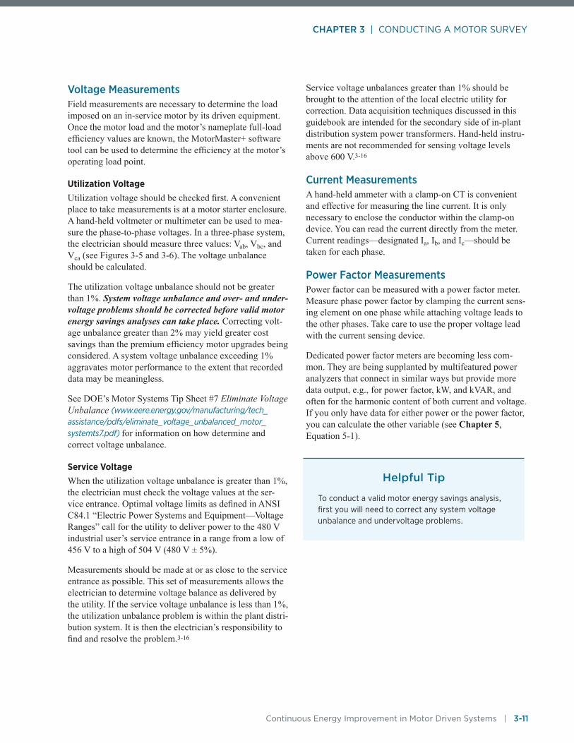
CHAPTER 3 | CONDUCTING A MOTOR SURVEY
Continuous Energy Improvement in Motor Driven Systems | 3-11
Voltage MeasurementsField measurements are necessary to determine the load imposed on an in-service motor by its driven equipment. Once the motor load and the motor’s nameplate full-load efficiency values are known, the MotorMaster+ software tool can be used to determine the efficiency at the motor’s operating load point.
Utilization VoltageUtilization voltage should be checked first. A convenient place to take measurements is at a motor starter enclosure. A hand-held voltmeter or multimeter can be used to mea-sure the phase-to-phase voltages. In a three-phase system, the electrician should measure three values: Vab, Vbc, and Vca (see Figures 3-5 and 3-6). The voltage unbalance should be calculated.
The utilization voltage unbalance should not be greater than 1%. System voltage unbalance and over- and under-voltage problems should be corrected before valid motor energy savings analyses can take place. Correcting volt-age unbalance greater than 2% may yield greater cost savings than the premium efficiency motor upgrades being considered. A system voltage unbalance exceeding 1% aggravates motor performance to the extent that recorded data may be meaningless.
See DOE’s Motor Systems Tip Sheet #7 Eliminate Voltage Unbalance (www.eere.energy.gov/manufacturing/tech_ assistance/pdfs/eliminate_voltage_unbalanced_motor_ systemts7.pdf) for information on how determine and correct voltage unbalance.
Service VoltageWhen the utilization voltage unbalance is greater than 1%, the electrician must check the voltage values at the ser-vice entrance. Optimal voltage limits as defined in ANSI C84.1 “Electric Power Systems and Equipment—Voltage Ranges” call for the utility to deliver power to the 480 V industrial user’s service entrance in a range from a low of 456 V to a high of 504 V (480 V ± 5%).
Measurements should be made at or as close to the service entrance as possible. This set of measurements allows the electrician to determine voltage balance as delivered by the utility. If the service voltage unbalance is less than 1%, the utilization unbalance problem is within the plant distri-bution system. It is then the electrician’s responsibility to find and resolve the problem.3-16
Service voltage unbalances greater than 1% should be brought to the attention of the local electric utility for correction. Data acquisition techniques discussed in this guidebook are intended for the secondary side of in-plant distribution system power transformers. Hand-held instru-ments are not recommended for sensing voltage levels above 600 V.3-16
Current MeasurementsA hand-held ammeter with a clamp-on CT is convenient and effective for measuring the line current. It is only necessary to enclose the conductor within the clamp-on device. You can read the current directly from the meter. Current readings—designated Ia, Ib, and Ic—should be taken for each phase.
Power Factor MeasurementsPower factor can be measured with a power factor meter. Measure phase power factor by clamping the current sens-ing element on one phase while attaching voltage leads to the other phases. Take care to use the proper voltage lead with the current sensing device.
Dedicated power factor meters are becoming less com-mon. They are being supplanted by multifeatured power analyzers that connect in similar ways but provide more data output, e.g., for power factor, kW, and kVAR, and often for the harmonic content of both current and voltage. If you only have data for either power or the power factor, you can calculate the other variable (see Chapter 5, Equation 5-1).
Helpful Tip
To conduct a valid motor energy savings analysis, first you will need to correct any system voltage unbalance and undervoltage problems.
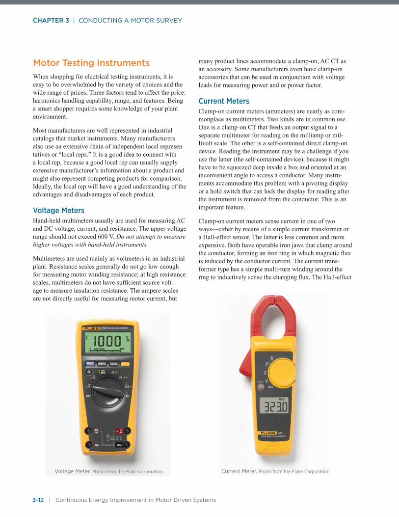
CHAPTER 3 | CONDUCTING A MOTOR SURVEY
3-12 | Continuous Energy Improvement in Motor Driven Systems
Motor Testing InstrumentsWhen shopping for electrical testing instruments, it is easy to be overwhelmed by the variety of choices and the wide range of prices. Three factors tend to affect the price: harmonics handling capability, range, and features. Being a smart shopper requires some knowledge of your plant environment.
Most manufacturers are well represented in industrial catalogs that market instruments. Many manufacturers also use an extensive chain of independent local represen-tatives or “local reps.” It is a good idea to connect with a local rep, because a good local rep can usually supply extensive manufacturer’s information about a product and might also represent competing products for comparison. Ideally, the local rep will have a good understanding of the advantages and disadvantages of each product.
Voltage MetersHand-held multimeters usually are used for measuring AC and DC voltage, current, and resistance. The upper voltage range should not exceed 600 V. Do not attempt to measure higher voltages with hand-held instruments.
Multimeters are used mainly as voltmeters in an industrial plant. Resistance scales generally do not go low enough for measuring motor winding resistance; at high resistance scales, multimeters do not have sufficient source volt-age to measure insulation resistance. The ampere scales are not directly useful for measuring motor current, but
many product lines accommodate a clamp-on, AC CT as an accessory. Some manufacturers even have clamp-on accessories that can be used in conjunction with voltage leads for measuring power and or power factor.
Current MetersClamp-on current meters (ammeters) are nearly as com-monplace as multimeters. Two kinds are in common use. One is a clamp-on CT that feeds an output signal to a separate multimeter for reading on the milliamp or mil-livolt scale. The other is a self-contained direct clamp-on device. Reading the instrument may be a challenge if you use the latter (the self-contained device), because it might have to be squeezed deep inside a box and oriented at an inconvenient angle to access a conductor. Many instru-ments accommodate this problem with a pivoting display or a hold switch that can lock the display for reading after the instrument is removed from the conductor. This is an important feature.
Clamp-on current meters sense current in one of two ways—either by means of a simple current transformer or a Hall-effect sensor. The latter is less common and more expensive. Both have operable iron jaws that clamp around the conductor, forming an iron ring in which magnetic flux is induced by the conductor current. The current trans-former type has a simple multi-turn winding around the ring to inductively sense the changing flux. The Hall-effect
Current Meter. Photo from the Fluke CorporationVoltage Meter. Photo from the Fluke Corporation
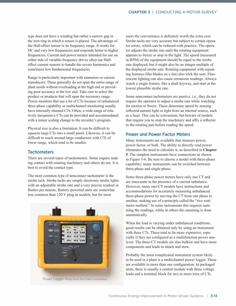
CHAPTER 3 | CONDUCTING A MOTOR SURVEY
Continuous Energy Improvement in Motor Driven Systems | 3-13
type does not have a winding but rather a narrow gap in the iron ring in which a sensor is placed. The advantage of the Hall-effect sensor is its frequency range. It works for DC and very low frequencies and responds better to higher frequencies. Current and power meters intended for use on either side of variable-frequency drives often use Hall-effect current sensors to handle the severe harmonics and sometimes low fundamental frequencies.
Range is particularly important with ammeters or current transducers. These generally do not span the entire range of plant needs without overloading at the high end or provid-ing poor accuracy at the low end. Take care to select the product or products that will span the necessary range. Power monitors that use a lot of CTs because of unbalanced three-phase capability or multichannel monitoring usually have internally shunted CTs. Often, a wide range of rela-tively inexpensive CTs can be provided and accommodated with a minor scaling change to the recorder’s program.
Physical size is also a limitation. It can be difficult to squeeze large CTs into a small panel. Likewise, it can be difficult to reach around large conductors with CTs of lower range, which tend to be smaller.
TachometersThere are several types of tachometers. Some require mak-ing contact with rotating machinery and others do not. It is best to avoid the contact type.
The most common type of noncontact tachometer is the strobe tach. Strobe tachs are simply electronic strobe lights with an adjustable strobe rate and a very precise readout in flashes per minute. Battery-powered units are somewhat less common than 120 V plug-in models, but for most
users the convenience is definitely worth the extra cost. Strobe tachs are very accurate but subject to certain opera-tor errors, which can be reduced with practice. The opera-tor adjusts the strobe rate until the rotating equipment appears to freeze or stop in the light. The speed (measured in RPM) of the equipment should be equal to the strobe rate displayed, but it might also be an integer multiple of the displayed strobe rate. Rotating equipment with repeat-ing features (like blades on a fan) also trick the user. Fluo-rescent lighting can also cause erroneous readings. Always watch a single feature, like a shaft keyway, and start at the lowest plausible strobe rate.
Some noncontact tachometers are passive, i.e., they do not require the operator to adjust a strobe rate while watching for motion to freeze. These determine speed by sensing reflected natural light or light from an internal source, such as a laser. This can be convenient, but beware of models that require you to stop the machinery and affix a reflector to the rotating part before reading the speed.
Power and Power Factor MetersMany instruments are available that measure power, power factor, or both. The ability to directly read power eliminates the need to calculate it, as described in Chapter 5. The simplest instruments have connections as shown in Figure 3-6. Be sure to choose a model with three-phase capability; many instruments can be switched between three-phase and single-phase.
Some three-phase power meters have only one CT and are inaccurate in the presence of a current unbalance. However, many one-CT models have instructions and accommodations for accurately measuring unbalanced three-phase power by moving the CT from one phase to another, making use of a principle called the “two watt meter method.” In some instruments this requires sum-ming the readings, while in others the summing is done automatically.
When the load is varying under unbalanced conditions, good results can be obtained only by using an instrument with three CTs. These tend to be more expensive, espe-cially if they are configured as a multifunction power ana-lyzer. The three-CT models are also bulkier and have more components and leads to attach and stow.
Probably the most complicated instrument system likely to be used in a plant is a multichannel power logger. These are available in more than one configuration. In packaged units, there is usually a central module with three voltage leads and a terminal block for two or more trios of CTs.
Power Logger. Photo from the Fluke Corporation

CHAPTER 3 | CONDUCTING A MOTOR SURVEY
3-14 | Continuous Energy Improvement in Motor Driven Systems
The central module is both a logger and a transducer; it computes power based upon voltage and the current from the CTs and records the power. All loads must be on the same voltage source, since there is only one set of voltage leads. CTs are marked by phase, so phase identification markings must be present at each load.
Among the many variations on the configuration above, some products consist of a central logger with remote power transducers. Interconnections typically follow voltage, current, or pulse conventions used in industrial programmable logic controller (PLC) systems. Often,
they can be equipped with a computer interface, phone modems, or radio transmitters for remote data retrieval. For some tiny battery-powered models, the logger is no bigger than the CTs that attach them. This can be very convenient in an industrial environment, because the entire logger can be closed up in the motor controller box for the monitoring period with no external power connection.
Motor AnalyzersA variety of products fall under the heading of “motor analyzers.” Several portable units recently appeared on the market to measure motor performance, including motor efficiency. Other efficiency analyzers have gone out of production, perhaps because of a market preference for analyzers oriented more toward predictive maintenance. Several current-signature analysis predictive maintenance analyzers that have entered North American markets have features for estimating efficiency.
All high-end analyzers have connections to the motor to sense current, voltage, and speed. Speed is sensed magnet-ically or optically. Certain nameplate information must be entered using a keyboard. These devices all require wind-ing resistance, which must be obtained when the motor is shut down; usually the required micro-ohmmeter is built into the tester. Most require no-load or low-load data, which must be obtained with the motor uncoupled and running at idle. Fortunately, none of them require any sort of torque sensor, because it would be nearly impossible to affix one in many field situations.
Motor analyzers are costly sophisticated products; dif-ferent models have different capabilities and operating requirements. They also vary as to difficulty of use. It is important to study alternatives carefully to find the best match for your budget and staff capabilities.
Metering technologies, equipment, and applications are discussed in DOE’s Federal Energy Management Program publication, Metering Best Practices: A Guide to Achiev-ing Utility Resource Efficiency (www.eere.energy.gov/femp/pdfs/mbpg.pdf). 3-18
Quick Fact
Power Quality Considerations
If variable-speed drives, induction heaters, or other electronic loads are on the system, expect the presence of voltage harmonics. Extreme current harmonics are present in circuits feeding these loads. The purchaser should describe this electrical environment to the equipment supplier and determine the ability of alternative devices to measure such “dirty” power accurately.
At a minimum, devices that sense voltage or current must operate on a true RMS principle. Those that do not will read inaccurately in the presence of harmonics.
Knowing that an instrument operates on a true RMS principle is not completely sufficient, however, as all instruments are limited by the magnitude and frequency of the harmonics they can handle while still reading accurately. One index of this capability is the crest factor, which is the ratio of peak value to RMS value of a wave form. A perfect sine wave has a crest value of 1.414. True RMS instruments should have a crest factor of 3.0 or better.
Unfortunately, crest value alone is not a complete descriptor of harmonic content. Harmonics caused by most electronic loads cause the current crest factor to be higher and the voltage crest factor to be lower than sinusoidal. An instrument needs to be able to measure accurately across the frequency range of the harmonics. The frequency of harmonics is expressed either in hertz (Hz) or in the order of harmonic. To convert order to frequency, simply multiply by 60. Most high-quality electrical testing instruments specify the frequency range over which their accuracy is maintained.

CHAPTER 3 | CONDUCTING A MOTOR SURVEY
Continuous Energy Improvement in Motor Driven Systems | 3-15
References 3-1 Advanced Energy, Motor Survey: How-To Guide,
1997.
3-2 Wayne Stebbins, “Motor Management Strategies,” Energy User News, June 1998.
3-3 Copper Development Association, Motor Management Best Practices, Part 1: Creating a Motor Inventory, Repair/Replacement Guidelines, March 2012.
3-4 Nailen, Richard L., “How to Conduct a Preliminary Motor Energy Audit,” Electrical Apparatus, March 1996.
3-5 Copper Development Association, Weyerhaeuser Policy Calls for Premium-Efficiency Motors and Transformers, A Copper Applications Case Study, A6080-XX/02, 2002.
3-6 Advanced Energy, “Solutions for Industry,” Metric Motors, June 1997.
3-7 Cowern, Howard H., Applications Engineer, Baldor Electric Company, “How to Change-Out Flange-Mount Metric Motors,” EC&M, July 1997.
3-8 Consortium for Energy Efficiency, The 1-2-3 Approach to Motor Management, prepared for Motor Decisions Matter, 2007.
3-9 Consortium for Energy Efficiency, Motor Planning Kit Version 2.1, Strategies, Tools, and Resources for Developing a Comprehensive Motor Manage-ment Plan, prepared for Motor Decisions Matter, 2007.
3-10 Agamloh, Emanuel, Kitt Butler, Nicole Kaufman, Ziba Kellum, Jeremy Morrison, and Dan Welch, Achieving More with Less: Efficiency and Econom-ics of Motor Decision Tools, Advanced Energy, March 2006.
3-11 Ula, Sadrul, Larry E. Birnbaum, and Don Jordan, Energy Efficient Drivepower: An Overview, Bonn-eville Power Administration, Western Area Power Administration.
3-12 Thompson, Mark E and Chris L. Dent, “PGE Drive Power Program Evaluation: The Accuracy of Customer-Provided Operating Hours and Motor Loading Assumptions,” 1994 American Council for an Energy-Efficient Economy (ACEEE) Summer Study on Energy Efficiency in Buildings, v. 8: Measurement and Evaluation, pp. 8.215–8.224.
3-13 McCoy, Gilbert A., Johnny Douglass, and Ron Major, Washington State University Energy Program, Motor Efficiency Improvements at the Bremerton Naval Complex: Motor Survey and NEMA Premium® Motor Replacement Analysis Results, prepared for the Bonneville Power Administration, March 2005.
3-14 McCoy, Gilbert A, and Johnny Douglass, Washington State University Energy Program, Motor Management Plan for the Domtar Kamloops Pulp Mill, prepared for BC Hydro, December 2007.
3-15 U.S. Department of Energy, Energy Efficient Electric Motor Selection Handbook, DOE/GO-10095-290, August 1996.
3-16 Carrol, Hatch & Associates, Inc., A Procedure for Developing an Energy Efficiency Plan for the Use of Industrial Motors in an Industrial Setting, June 1994.
3-17 Washington State University Extension Energy Program, MotorMaster+ 4.0 User Guide, prepared for DOE, 2003.
3-18 U.S. Department of Energy, Metering Best Practices: A Guide to Achieving Utility Resource Efficiency, August 2011.

Continuous Energy Improvement in Motor Driven Systems
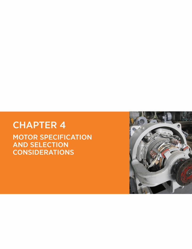
CHAPTER 4 MOTOR SPECIFICATION AND SELECTION CONSIDERATIONS

CHAPTER 4 | MOTOR SPECIFICATION AND SELECTION CONSIDERATIONS
4-2 | Continuous Energy Improvement in Motor Driven Systems
When specifying a motor, the purchaser must indicate the desired motor horsepower rating, nominal voltage, synchronous speed, enclosure type, frame size, insula-tion class, and efficiency class (or minimum full-load efficiency value). For some applications, definite or spe-cial purpose motors are required. This chapter discusses motor choices, performance, and associated efficiency implications.
Motors drive many kinds of loads, which vary greatly as to what they require of the motors. For example, the driven equipment might provide constant fluid flow and be powered by a constant speed general purpose motor. Alternatively, the driven equipment could provide vari-able flows with flow control provided by an inverter-duty motor controlled by an adjustable speed drive. Loads also might create a constant or cyclic torque demand at a given speed. In comparison to its running torque, a load might have high inertia and require high starting and accelerating torque. The motor might operate in a hostile environment where temperature, humidity, dust, or industrial chemicals are present. And it might need to operate continuously or only occasionally. For every load, a motor must be chosen that can successfully start and run under all conditions—one that can endure the stresses of the specific environ-ment and operating requirements. And it must do this at the lowest possible life cycle cost.
Mandatory Motor Full-Load Efficiency StandardsMandatory minimum full-load motor efficiency standards currently in effect in the United States have been estab-lished through two pieces of legislation:
• Energy Independence and Security Act of 2007 (EISA)
• EPAct
The initial set of federal mandatory commercial and industrial motor performance standards were created by the EPAct. By October 1997, new general-purpose, three-phase induction motors and most definite-purpose motors sold in the United States had to equal or exceed the energy efficient motor full-load efficiency levels prescribed by the EPAct. These efficiency levels were identical with those given in Table 12-6c of NEMA Standard Publication MG 1-1989 Motors and Generators. Motors with full-load effi-ciency values below the energy efficient standards were deemed “standard efficiency” motors.
The EPAct applied to single speed, general purpose, T-frame, continuous rated, foot-mounted, polyphase, squirrel-cage induction motors of NEMA Designs A and B. Ratings covered under the legislation include 1 to 200 hp; 230/460 V; 3,600, 1,800, and 1,200 RPM motors in open and closed enclosures. These standards applied to motors manufactured alone and as a component of another piece of equipment.4-1, 4-2
After the mandatory EPAct standard was established, NEMA in 1994 extended the coverage of the “energy effi-cient” efficiency standard through 500 hp and renumbered Table 12-6c (it is currently referred to as Table 12-11). From 250 to 500 hp, the term “energy efficient” still desig-nates relatively high-efficiency motors.
In August 2001, NEMA introduced a premium energy effi-ciency motor standard. Under its program, a motor may be marketed as a premium motor if it meets or exceeds a set of NEMA nominal full-load efficiency levels as defined in NEMA MG 1-2011, Tables 12-12, 12-13, 20-B, and 20-C. These levels are higher than the minimum full-load effi-ciency standards for energy efficient motors incorporated into the EPAct and listed in MG 1-2011, Table 12-11, and 20-A.
Premium efficiency motor standards apply to NEMA Design A and B, three-phase low voltage induction motors rated from 1 hp to 500 hp and designed for service at 600 V or less (see Table 12-12 of NEMA MG 1-2011). Cov-ered products include foot-mounted motors with speeds of 3,600, 1,800, 1,200, and 900 RPM with ODP, explo-sion-proof, and TEFC enclosures. Also covered under the standard are severe-duty, washdown, IEC metric frame motors, and brake motors.
A second premium efficiency standard was developed for medium voltage motors (form wound, rated for service at 5,000 V or less). Minimum nominal full-load efficiency values apply to open and enclosed motors rated from 250 hp to 2,500 hp and with synchronous speeds of 3,600, 1,800, 1,200, and 900 RPM (see Table 12-13, 20-B, and 20-C of NEMA MG 1-2011).
Under EISA, the mandatory minimum nominal full-load efficiency for low-voltage general-purpose motors with a power rating up to 200 hp was raised to the premium efficiency level as given in Table 12-12 of NEMA MG 1-2011. The premium efficiency requirement applies to motors purchased alone, imported into the country, or purchased as a component of another piece of equipment. EISA is much more stringent than EPAct.

CHAPTER 4 | MOTOR SPECIFICATION AND SELECTION CONSIDERATIONS
Continuous Energy Improvement in Motor Driven Systems | 4-3
EISA also requires NEMA Design B motors with power ratings between 201 and 500 hp to have a full-load effi-ciency that meets or exceeds the NEMA energy efficient motor standards (given in Table 12-11 of NEMA MG 1-2011). End users may voluntarily purchase premium efficiency Design B motors in these ratings. The EISA motor efficiency standards took effect in December 2010. Canadian national motor efficiency standards mostly match the EISA requirements (except that they cover all motors rated at <600 V instead of 230/460 V motors).
EISA also expanded the term “general purpose” motor to include a number of motor subtypes that were not covered by the earlier EPAct motor efficiency standards. These motors now must have full-load efficiency values that meet or exceed the NEMA energy efficient motor stan-dards given in Table 12-11 of NEMA MG 1-2011. Motors in the 1 hp to 200 hp ratings that are covered by this man-datory minimum full-load efficiency standard include:4-3, 4-4
• U-frame motors
• Design C motors
• Close-coupled pump motors
• Footless (C-face or D-flange without base) motors
• Vertical solid shaft normal thrust motors (P-base)
• Eight-pole (900 RPM) motors
• Polyphase motors with a voltage of not more than 600 V (other than 230 V or 460 V motors). This applies to 200 V and 575 V motor model lines
• Fire pump motors.
Motor efficiency standards are constantly evolving, both in the United States and overseas. The IEC has proposed an above premium efficiency (or IE4) standard level. The minimum full-load efficiency values under discussion may exceed the performance capability of AC induction motor technology.4-5
In March 2010, DOE adopted energy efficiency standards for fractional horsepower polyphase and single-phase motors. These standards cover motors operating at 3,600, 1,800, and 1,200 RPM and include capacitor-start/induc-tion run and capacitor-start/capacitor run open motors rated between 0.25 hp and 3 hp. These standards will be applicable beginning March 2015.4-6
Nameplate Efficiency Labeling ProtocolsEnergy efficiency, annual operating hours, and motor load are the main factors that determine the lifetime cost of owning and operating a motor. Energy costs typically exceed initial motor purchase costs within a year of con-tinuous operation. NEMA Standard MG1 requires that a “nominal” full-load efficiency value appear on the motor nameplate. This nominal efficiency must be derived from tests conducted in accordance with IEEE Standard 112, test method B. The nameplate efficiency represents the efficiency at full-rated load with all three phases at nomi-nal voltage.
Motors not Covered by EISA4-4
■■ Single-phase motors
■■ DC motors
■■ Two-digit frames (42-48-56)
■■ Multispeed motors
■■ Medium voltage motors
■■ Totally enclosed non-ventilated (TENV) and TEAO enclosures
■■ Motors with customized original equipment manufacturer (OEM) mountings
■■ Intermittent duty motors
■■ Submersible motors
■■ Encapsulated motors
■■ Motors that are integral with gearing or brake where the motor cannot be used separately
■■ Design D motors
Helpful Tip
Always replace single-phase motors with three-phase motors when possible.4-4
Full-load efficiency values for a 5 hp 1,800 RPM motor are given below:
■■ Typical Single Phase: 80.0%
■■ Premium Single Phase: 86.5%
■■ Premium Three Phase: 90.2%

CHAPTER 4 | MOTOR SPECIFICATION AND SELECTION CONSIDERATIONS
4-4 | Continuous Energy Improvement in Motor Driven Systems
A somewhat complex set of procedures is used to deter-mine the exact nominal efficiency that will appear on the nameplate for each model line. IEEE 112B testing is con-ducted on a population of motors within each model line, and an “average efficiency” is determined as the arithmetic mean efficiency of that population. NEMA recognizes that manufacturing tolerances will lead to variations in effi-ciency for individual motors within a population. NEMA has confronted this issue by defining a lower “minimum” efficiency that must be equaled or exceeded by all motors in a motor model line.
One might expect that the nominal (nameplate) efficiency would be the same as the average efficiency, but it is not. NEMA MG 1 has established efficiency bands topped by specific nominal efficiencies that can be placed on the nameplate. Those bands are reproduced here as Table 4-1. After determining the actual average efficiency, the manu-facturer must label the motor with a nominal efficiency from the table that is equal to or less than the average efficiency. For every nominal efficiency band, the table contains a corresponding minimum efficiency value.
The purchaser can be comfortable using NEMA nominal efficiency from the nameplate in making motor purchasing decisions. This is not to imply that all new motors arrive free of manufacturing flaws that reduce efficiency and other performance parameters. Such flaws appear periodi-cally, and purchasers should conduct receiving inspection tests to check for them. Record nameplate information into your motor tracking system when new motors are delivered.
For nearly every category and rating of motor there are multiple manufacturers, and each one offers several mod-els. The various models span a range of nominal efficien-cies. It is important to know what efficiencies are avail-able within each group of competing models and how to specify the highest economically justifiable efficiency. This task is made easier by the adoption of mandatory minimum full-load efficiency standards. Standards also provide a basis for various premium or enhanced effi-ciency motor rebate or incentive programs sponsored by electric utilities.
Horsepower RatingsMotor “size” generally implies a shaft output power or horsepower rating. IEC metric motors are rated in kW. Motors can be oversized and still serve a load satisfac-torily and (to a point) efficiently. They deliver the horse-power the load requires, not their rated horsepower. Most motors above the fractional horsepower range maintain a
Table 4-1. Motor Nameplate Efficiency Marking Standard. Source NEMA MG 1-2011, Table 12-10
Nominal Efficiency
Minimum Efficiency
Nominal Efficiency
Minimum Efficiency
99.0 98.8 91.0 89.5
98.9 98.7 90.2 88.5
98.8 98.6 89.5 87.5
98.7 98.5 88.5 86.5
98.6 98.4 87.5 85.5
98.5 98.2 86.5 84.0
98.4 98.0 85.5 82.5
98.2 97.8 84.0 81.5
98.0 97.6 82.5 80.0
97.8 97.4 81.5 78.5
97.6 97.1 80.0 77.0
97.4 96.8 78.5 75.5
97.1 96.5 77.0 74.0
96.8 96.2 75.5 72.0
96.5 95.8 74.0 70.0
96.2 95.4 72.0 68.0
95.8 95.0 70.0 66.0
95.4 94.5 68.0 64.0
95.0 94.1 66.0 62.0
94.5 93.6 64.0 59.5
94.1 93.0 62.0 57.5
93.6 92.4 59.5 55.0
93.0 91.7 57.5 52.5
92.4 91.0 55.0 50.5
91.7 90.2 52.5 48.0
50.5 46.0

CHAPTER 4 | MOTOR SPECIFICATION AND SELECTION CONSIDERATIONS
Continuous Energy Improvement in Motor Driven Systems | 4-5
high efficiency to about 50% load. You can find full and part-load efficiencies down to 25% of full-load in Motor-Master+. There are some advantages to moderate motor oversizing. You have a greater margin of safety from over-heating, a “cushion” to accommodate errors in estimat-ing or load spikes, faster acceleration to operating speed, greater tolerance to undervoltage operation, and poten-tially higher efficiency.
Motors typically operate at their highest efficiency when loaded to about 70% to 80% of full-load. This perfor-mance characteristic occurs because above 60% load the motor’s shaft or output horsepower varies linearly with current. Resistance losses, however, vary with respect to the square of the current. Motor efficiency is equal to out-put (output + losses) and efficiency increases when resis-tance losses are reduced faster than the delivered output.
Underloaded motors operate at lower power factor, although this disadvantage is minor if power factor is cor-rected with capacitors, low power factor is not penalized by the utility, or the motor is controlled by an adjust-able speed drive that corrects for power factor. Oversized motors draw more current because of their reduced power factor at part-load. In addition, they draw a higher start-ing current, because starting current is a property of the motor and is not affected by the magnitude of the load. Motor efficiency and power factor as a function of load are shown in Figure 1-1. Oversized motor performance is discussed in detail in AMO’s Premium Efficiency Electric Motor Selection and Application Guide.4-7
Synchronous SpeedAC motor speed is controlled primarily by the stator wind-ing configuration, which determines the number of mag-netic poles in the stator. The rotational speed of the mag-netic field is known as the motor’s synchronous speed, and it is always 120 times the line frequency divided by the number of poles. Wherever a 60 Hz line frequency is used, this works out to speeds of 3,600 RPM (two poles), 1,800 RPM (four poles), 1,200 RPM (six poles), and 900 RPM (eight poles). In countries with a 50 Hz power sup-ply, 2-, 4-, 6- , and 8-pole motors would rotate at 3,000, 1,500, 1,000, and 750 RPM, respectively.
For all AC motors except the commonplace induction motor, rotor and shaft speed are exactly the same as synchronous speed. Induction motors have slip; they run slower by a few percent than synchronous speed. That is why induction motor nameplate full-load speeds are a little lower than the motors’ synchronous speeds.
Slip is the difference between a motor’s synchronous speed and its operating speed. The motor’s full-load speed is its synchronous speed less the slip that occurs when the motor is fully loaded. Slip varies from less than 1% of synchronous speed for large premium efficient motors (and lightly loaded motors) to greater than 5% for many fractional horsepower motors and motors used in special applications. Slip represents one of several energy loss categories in a motor. For this reason, induction motor designers try to keep slip low; however, manufacturing costs and other operating parameters, like starting current and torque, tend to move in the wrong direction if slip is too low.
Synchronous speed minus the slip is the motor operating speed. Operating speed is very important in centrifugal pump and fan applications where input power require-ments are speed sensitive. For centrifugal fans and cen-trifugal circulating water pumps (i.e., pumps used in a non-static lift application), fluid flow is proportional to the shaft speed; the power requirement, however, is propor-tional to the cube of the shaft speed. Even small speed differences are significant as a 1% increase in operating speed shifts the fan or pump performance curve so the system curve intersects it at different location. The result is higher flow, and a higher discharge or outlet pressure resulting in an overall 3% power increase. Energy use increases even in applications like a pump filling a tank—where the tank will be filled in less time.
For a given motor, speed and slip are not constant; they vary with load and voltage. See Chapter 5 for information on determining motor load from measurements of its speed.
Full-Load and Locked-Rotor TorqueAll motors of the same horsepower and speed rating have the same full-load torque. They differ, however, in the torque they can provide at start-up and throughout accel-eration. NEMA has several three-phase induction motor design designations, denoted by the letters A, B, C, and D. These should not be confused with other parameters that NEMA also classifies by letter, such as locked-rotor current and insulation temperature tolerance. A variety of motor performance parameters are set by the design letter, horsepower rating, and synchronous speed of a motor, but the most important is the minimum delivered torque at start-up and during acceleration of the motor. Figure 4-1 shows typical torque-speed curves during acceleration of motors of different NEMA designs.

CHAPTER 4 | MOTOR SPECIFICATION AND SELECTION CONSIDERATIONS
4-6 | Continuous Energy Improvement in Motor Driven Systems
At the moment acceleration begins, the torque developed is called the “locked-rotor torque.” For motors in the NEMA Design A, B, and C categories, torque actually drops somewhat as acceleration begins and reaches some minimum value, which is still higher than the steady-state torque at rated load and speed. This minimum is called the “pull-up” torque. As acceleration proceeds, a torque maxi-mum called the “breakdown” torque is reached. The load also has a speed torque curve. When overlaid, the motor torque curve must be greater than the load torque curve at every speed point. Otherwise, the motor will overload and stall before reaching its breakdown torque.
Even within a NEMA Design letter category, motor models of the same rating can differ in locked rotor and accelerating torque—remember that NEMA only specifies minimum locked rotor and pull-up torque values that a motor must equal or exceed. If starting or accelerating torque is criti-cal, you can obtain measured locked rotor torque values from manufacturer’s data or from MotorMaster+.
NEMA has placed a maximum limit on the starting current of Design B, C, and D motors (which are the most com-mon). Design A motors are quite similar in performance to a Design B motor, but there is no limit on starting current. Design C motors are designed for higher starting torque and are most often used in material handling applications,
when an initial high torque is needed to overcome static friction or material compaction. Design A through C motors all have the same maximum allowable slip, but Design C motors tend to exhibit higher slip within that limit.
Design D motors are high-slip machines for use on loads that cycle several times per minute in their torque demand. Such applications include punch presses and rocking beam oil well pumps. In these applications, a flywheel is used to supplement the motor through the high torque moments; otherwise, it would stall. The flywheel decelerates as a result of contributing momentum to the load shaft during the high torque moments. The motor re-accelerates the flywheel during the low torque demand part of the cycle. Figure 4-1 makes it clear that designs other than Design D would reach a breakdown torque with very little decelera-tion of the load. A Design D motor’s breakdown torque is essentially the same as its locked-rotor torque.
Never use a Design C or D motor in an application where a Design A or B motor would work because Designs C and D motors are considerably less efficient.
Full-Load and Locked-Rotor CurrentA motor’s full-load current or amperage rating is impor-tant for sizing the electrical service and protection. At rated load, the current rating is listed on the nameplate in amperes. For multivoltage motors, the amperages for each connectable voltage are given in the same sequence as the voltages to which they correspond.
It is very important to provide for the high locked-rotor current that occurs when a motor starts and acceler-ates. Locked-rotor current varies but tends to be around six times the rated full-load current. The code letter that pertains exclusively to locked-rotor current is usually just designated “Code” on the nameplate, and it should not be confused with the NEMA Design letter. These letter codes are associated with a range of kVA per rated horsepower.
To determine the actual locked-rotor amperage rating, obtain the code letter from the nameplate or catalog and look up the kVA per horsepower (kVA/hp) correspond-ing with the code letter from Table 4-2, which has been taken from NEMA MG 1. Next, multiply the table number by the rated horsepower of the motor and then divide by 1.732 times the motor voltage rating in kV, e.g., 0.46 kV for a 460 V motor. MotorMaster+ provides the locked-rotor or starting current for new motors directly in amps. For multi-voltage rated motors, MotorMaster+ lists the
Speed (Percent synchronous speed)
Torq
ue (
perc
ent o
f ful
l-lo
ad to
rque
)
20 40 80 10060
A or B
C
D
0
100
0
300
200
Figure 4-1. Torque-Speed Curves for NEMA Design A-D Motors

CHAPTER 4 | MOTOR SPECIFICATION AND SELECTION CONSIDERATIONS
Continuous Energy Improvement in Motor Driven Systems | 4-7
full-load and locked-rotor amperage for the highest volt-age connection. The amperage is inversely proportional for other potential utilization voltages, e.g., if the full-load current is 50 amps with the 460 V connection, it will be 100 amps with a 230 V connection.
With the efficiency improvements of the last several years, NEMA and the National Electrical Code (NEC) have dealt with one more important category of motor current. This is the instantaneous inrush current, and it should be care-fully distinguished from locked-rotor current. Locked-rotor current is an RMS current, which means current has to have been established for at least one full AC cycle before it can be defined or measured. Instantaneous inrush current is the peak instantaneous current that occurs on any phase within the first half-cycle after starting contacts close.
A premium efficient motor is liable to have a greater instantaneous inrush current than a standard efficient counterpart with the same locked-rotor current. No NEMA Design limits instantaneous inrush current although many Design B motors must be reclassified as NEMA Design A motors when redesigned as a premium efficient motor.
This is of no consequence in most situations because of its brief duration. But inrush current can be a problem in situ-ations where so-called instantaneous magnetic-only circuit protectors are used. If nuisance tripping occurs after an efficiency upgrade where instantaneous circuit protectors are used, consult Section 430 of the latest revision of the NEC. The code has been modified to allow adjustments to a higher trip setting when nuisance tripping occurs. For additional information, see DOE Motor Systems Tip Sheet #6, Avoid Nuisance Tripping with Premium Efficiency Motors (www.eere.energy.gov/manufacturing/tech_ assistance/pdfs/avoid_nuisance_motorsys_ts6.pdf).
Frame SizeMotor frame sizes were not standardized prior to 1952. In 1952, NEMA established a set of standards for U-frame motors. As upgraded insulation systems were developed, T-frame motor standards were introduced in 1964. T-frame motors are smaller than U-frame motors of a comparable horsepower rating. U-frame motors can be identified by the frame designation on the motor nameplate (for 1- to 100-hp motors, 182, 184, 213, 215, 254U, 256U, 284U, 324U, 326U, 364U, 365U, 404U, 405U, 444U, 445U). T-frame motors have the letter “T” following the frame number (i.e., 143T, 145T, 182T, 184T, 213T, 215T, 254T, 256T, 284T, 284T, 324T, 326T, 364T, 365T, 404T, 405T). A frame number ending in TC designates a ‘C-face’ motor, while LP, HP, or VP indicates a P-base or vertical shaft motor. Close-coupled pump motors have frame numbers ending with JP or JM.
For small machines, the frame number is 16 times the dis-tance of the shaft centerline height above the motor base-plate (when measured in inches). For larger machines (140 frame and above), the first two digits of the frame number are four times the distance that the shaft height is above the motor baseplate (when measured in inches). With IEC motors, the frame designation indicates the shaft height in millimeters (mm).
To be assured of a proper fit without having to modify the mounting, purchase replacement motors with the same frame size designation as that of the original motor. Pre-mium efficiency T-frame and U-frame motors are avail-able in the same range of frame sizes as the older motors they replace. Frame size is predominantly associated with the dimensions of all mounting and contact surfaces, including the shaft height and diameter.
While premium efficiency U-frame motors are available, they are considerably more expensive than equivalent rated T-frame motors. Frame adapters or transition bases
Table 4-2. NEMA Locked-Rotor Code Letter Definitions
Letter Designation kVA/hp* Letter
Designation kVA/hp*
A 0.00–3.15 K 8.0–9.0
B 3.14–3.55 L 9.0–10.0
C 3.54–4.0 M 10.0–11.2
D 4.0–4.5 N 11.2–12.5
E 4.4–5.0 P 12.4–14.0
F 5.0–5.6 R 14.0–16.0
G 5.5–6.3 S 16.0–18.0
H 6.3–7.1 T 18.0–20.0
J 7.1–8.0 U 20.0–22.4
V 22.5 and up
*The locked kVA per horsepower range includes the lower figure up to, but not including, the higher figure. For example, 3.14 is designated by letter A and 3.15 by letter B.

CHAPTER 4 | MOTOR SPECIFICATION AND SELECTION CONSIDERATIONS
4-8 | Continuous Energy Improvement in Motor Driven Systems
are available so that old U-frame motors can be replaced by premium efficiency T-frame motor models. The transi-tion bases accommodate the mounting bolts for both the T-frame and U-frame motors and line the T-frame motor shaft height up with the driven equipment shaft.4-8 Some industries have replaced all of their older U-frame with modern T-frame motors to reduce their spares inventory.
Some exterior dimensions that do not pertain to mount-ing are not controlled by frame size, so take care that your new motor does not interfere with structures having close clearances. Premium efficient motors sometimes extend beyond the opposite-drive-end mounting feet.
Enclosure TypeVarious enclosure designations pertain to the design fea-tures that facilitate the cooling of the motor and protect it from the surrounding environment. The most common NEMA enclosures are TEFC and ODP. NEMA’s MG 1 describes the circumstances and criteria for using each type of enclosure. Basically, an ODP enclosure permits the passage of cooling air around the windings of the machine. The ventilation openings are constructed so operation is not interfered with when drops of liquid or solid particles strike the enclosure at any angle from 0° to 15° from the vertical. A TEFC machine is enclosed to prevent the exchange of cooling air between the inside and outside of the enclosure. The TEFC enclosure is designed to prevent dust from interfering with machine operation. NEMA also includes a “suggested standard for future design” that follows the lead of the IEC. The IEC ingress protection (IP) enclosure rating approach assigns numeric values that indicate the degree of protection against intru-sion of solid objects and the ingress of liquids. For most industrial applications, IP22 relates to ODP motors, IP54 to TEFC, IP45 to weatherproof, and IP55 to washdown duty motors.4-9
Hazardous location is another important type of motor enclosure (often referred to as “explosion-proof” motors by manufacturers). They are designed for use in harsh industrial environments that contain hazardous gas and vapor that may have explosive properties. A common misperception is that explosion-proof motors are sealed so tightly that no dust or other contaminants can enter. This is not true. The motor can breathe as the air inside expands and contracts, just as a TEFC motor does. The explosion-proof motor has a “flame path” at the endplate to frame joint to quench any flames from an internal fire or arcing fault before it can propagate and ignite flammables in the air surrounding the motor.
Explosion-proof motors are designated under the NEC as compatible for use in Class 1 Group C and D environ-ments, or are rated for operation in Class II Group E, F, and G environments. Equivalent IEC motors are desig-nated as “flame-proof” motors.4-9 Premium efficiency explosion-proof motors are available from most manu-facturers. Always make sure that a standard efficiency explosion-proof motor is replaced by a premium efficiency motor that is rated for the same environment.
Additional enclosure types include totally enclosed non-ventilated (TENV), TEAO, totally enclosed blower-cooled (TEBC), and weather protected (WP).
Insulation ClassNEMA has established standards for motor insulation system design, temperature rating, and motor thermal capacity. Four classes of insulation are available, each with an allowable temperature rise above ambient (ambi-ent is defined as 40ºC or 104ºF) and maximum allowable temperature. A motor’s insulation class is a system rating based on insulation materials including the wire coatings, varnish, slot liners, lead wire insulation, and topsticks. Motor insulation systems are based on temperature endur-ance for 20,000 hours and are designated as class A, B, F, or H. Class A insulation systems are shown by experience or test to have a suitable operating life when operated at a maximum temperature of 105ºC. A Class B system shows acceptable thermal life when operated at 130ºC; a Class F system can be operated at a limit of 155ºC; while a Class H system can be operated at a limiting temperature of 180º C.4-1 Class A insulation is rarely used today; Class B is the “baseline” insulation system; while Class F insulation is considered standard for most energy efficient and pre-mium efficiency motors.
Because a motor is supplied with a Class F or H insulation system does not mean that the motor’s actual temperature rise or operating temperature increases. A higher insula-tion class can result in an improved insulation life. The life of the insulation doubles for every 10ºC cooler the motor runs relative to its maximum thermal limits.

CHAPTER 4 | MOTOR SPECIFICATION AND SELECTION CONSIDERATIONS
Continuous Energy Improvement in Motor Driven Systems | 4-9
Service FactorThe service factor of an AC motor is a multiplier which, when applied to the rated motor horsepower, indicates a permissible loading for continuous operation at rated load under usual service conditions. While operation within the service factor is permissible, it is not recommended as a motor operating continuously at any service factor greater than 1 will have a reduced life expectancy. Both insulation life and bearing life are reduced by service factor loads. Most general purpose motors have a service factor of 1.15. This service factor is reduced to 1.0 when the motor is controlled by an electronic pulse-width modulated vari-able frequency drive.
Definite and Special Purpose MotorsA general purpose motor is an AC induction motor designed according to NEMA (or IEC) standards to meet a broad variety of applications. A definite purpose motor is produced in standard ratings and with standard operat-ing characteristics for particular applications or other than usual service conditions.
A special purpose motor is designed with special operat-ing characteristics for a particular application. Examples include inverter-duty motors, brake motors, and integral gear motors.
CHAPTER 4 | MOTOR SPECIFICATION AND SELECTION CONSIDERATIONS
4-10 | Continuous Energy Improvement in Motor Driven Systems
References 4-1 U.S. Department of Energy, Energy Efficient
Electric Motor Selection Handbook, August 1996.
4-2 GE Motors, “Energy Policy Act of 1992 as it Relates to Motors,” Industry Information, GEK-100919, 1993.
4-3 U.S Department of Energy “The 2007 Energy Act: Good News for Motor Users,” Energy Matters, Summer 2008.
4-4 Malinowski, John, Baldor Electric Company, Electrical Efficiency: Spec the Right Motor and Drive for Lifecycle Performance, November 2011.
4-5 Brunner, Conrad, Anibal de Almeida, Rob Boteler, Martin Doppelbauer, and William Hoyt, Motor MEPS Guide, February 2009.
4-6 U.S. Department of Energy, “Energy Conservation Program: Energy Conservation Standards for Small Electric Motors; Final Rule,” Federal Register, March 9, 2010.
4-7 U.S. Department of Energy, Premium Efficiency Electric Motor Selection and Application Guide.
4-8 Copper Development Association, Motor Man-agement Best Practices, Part II: Motor Failure Policies, and Purchasing Specifications, A6148-12, March 2012.
4-9 Clarke, Ron, Leeson Electric Corporation, How to Speak Fluent IEC for Motors.

CHAPTER 5 MOTOR LOAD AND EFFICIENCY ESTIMATION TECHNIQUES

CHAPTER 5 | MOTOR LOAD AND EFFICIENCY ESTIMATION TECHNIQUES
5-2 | Continuous Energy Improvement in Motor Driven Systems
To compare the operating costs of an existing standard efficient motor against those of a premium efficient replacement unit, you must determine operating hours, motor load, and the efficiency of each motor at its load point. Part-load is a term used to describe the actual load served by the motor in comparison to the ability of the motor to deliver shaft horsepower at its rated full load. The actual motor load can be estimated using input power, amperage, or speed measurements. Several load estima-tion techniques are briefly summarized.
Input Power MeasurementsWhen “direct-read” power meters are available, use them to measure the input power supplied to the motor and the load that is imposed upon the motor by the driven equip-ment. With measured parameters taken from hand-held
instruments, you can use Equation 5-1 to calculate the three-phase input power to the loaded motor. You can then quantify the motor’s part-load by comparing the measured input power when operating under load with the power that would be required if the motor was to operate at rated capacity (from Equation 5-2). The relationship that estimates motor loading based on power measurements is shown in Equation 5-3.
P = V × I × PF × √3
1000
Where:
P = Three phase power in kW
V =RMS voltage, mean line-to-line of three phases
I = RMS current, mean of three phases
PF = Power factor as a decimal
PR = HP × 0.7457
ηR
Where:
PR = Input power at full rated load in kW
HP = Nameplate rated horsepower
ηR = Efficiency at full rated load
Equation 5-1. Using Field Measurements to Determine Motor Input Power
Equation 5-2. Calculating the Full-Load Motor Input Power
An existing motor is a 40-hp, 1,800-RPM unit with an open drip-proof enclosure. The motor is 12 years old, has a full-load efficiency of 90.2%, and has not been rewound. The electrician makes the following measurements:
Measured Values:
Vab = 467 Volts Ia = 36 Amperes (A) PFa = 0.75
Vbc = 473 V Ib = 38 A PFb = 0.78
Vca = 469 V Ic = 37 A PFc = 0.76
Average Voltage = (467 + 473 + 469)/3 = 469.7 V
Average Current (I) = (36 + 38 + 37)/3 = 37 A
Power Factor (PF) = (0.75 + 0.78 + 0.76)/3 = 0.763
Equations 5-1 through 5-3 reveal that:
Input Power P = 469.7 × 37 × 0.763 × √3 / 1000 = 22.9 kW
Power at Rated Load PR = 40 × 0.7457 / 0.902 = 33.1
Load = P / PR = (22.9 / 33.1) × 100% = 69.3%
LOAD = P
× 100%PR
Where:
Load =Output power as a % of nameplate rated power
P = Measured three phase power in kW
PR = Input power at full rated load in kW
Equation 5-3. Estimating Motor Load using the Input Power Measurements
Example 5-1. Input Power and Load Calculations

CHAPTER 5 | MOTOR LOAD AND EFFICIENCY ESTIMATION TECHNIQUES
Continuous Energy Improvement in Motor Driven Systems | 5-3
Line Current MeasurementsThe current load estimation method is recommended when only voltage and amperage measurements are available. The amperage draw of a motor varies linearly with respect to load, down to about 50% of full load (see Figure 5-1). Below the 50% load point, power factor degrades due to reactive magnetizing current requirements and the amper-age curve becomes increasingly nonlinear. Below 50% load, current measurements are not a useful indicator of motor load.
Both nameplate full-load and no-load current values apply only at the rated motor voltage. Thus, RMS current mea-surements should always be corrected for over- or under-voltage. If the utilization voltage is below that indicated on the motor nameplate, the measured amperage value is correspondingly higher than expected under rated condi-tions and must be adjusted downwards. The converse is true if the supply voltage at the motor terminals is above the motor rating. Equation 5-4 shows the relationship of motor load to measured current values.
The Slip MethodAs noted earlier, the actual speed of the motor is less than its synchronous speed, with the difference between the synchronous and measured motor operating speed referred to as slip. The amount of slip is proportional to the load imposed on the motor by the driven equipment. Motor rotational speed measurements are generally easy to obtain with a contact tachometer or a strobe light as most motors are constructed so that the shaft is accessible.
The primary reasons to use the slip method to determine motor load are simplicity and safety advantages.5-1 While the voltage-compensated slip method is attractive for its simplicity, it lacks accuracy. The slip method is generally not recommended for determining motor loads in the field and should be used only when motor voltage and operat-ing speed measurements are available.
Perc
ent o
f Rel
ated
Loa
d V
alue
Percent of Full Load
100%
90%
80%
70%
60%
50%
40%
30%
20%
10%
10% 20% 30% 40% 50% 60% 70% 80% 90% 100%
Power Factor
Current
Power
0%
Figure 5-1. Relationships Between Power, Current, Power Factor, and Motor Load. Illustration from EM4MDS
Load = ( I×
V ) × 100%IR VR
Where:
Load = Output power as a % of rated power
I = RMS current
IR = Nameplate rated current
V =RMS voltage, mean line-to-line of three phases
VR = Nameplate rated voltage
Equation 5-4. Voltage Compensated Amperage Ratio Motor Load Estimation Technique

CHAPTER 5 | MOTOR LOAD AND EFFICIENCY ESTIMATION TECHNIQUES
5-4 | Continuous Energy Improvement in Motor Driven Systems
The synchronous speed of an induction motor depends on the frequency of the power supply and on the number of poles for which the motor is wound. The higher the frequency, the faster a motor runs. For a given frequency, the more poles the motor has, the slower it runs. Table 5-1 indicates typical synchronous speeds.
The motor load can be estimated with slip measurements as follows (see Equation 5-5 and Example 5-2).
The accuracy of the slip method is limited by multiple fac-tors. The largest uncertainty relates to the 20% tolerance that NEMA allows manufacturers in reporting nameplate full-load speed.5-1 Given this broad tolerance, manufactur-ers generally round their reported full-load speed values to some multiple of 5 RPM. Although 5 RPM is a small percentage of the full-load speed and might be consid-ered insignificant, the slip method relies on the difference between full-load nameplate and synchronous speeds.
LOAD = SLIP
× 100%(SS − SR )
Where:
Load = Output power as a % of rated power
Slip =Synchronous speed – measured speed in RPM
SS = Synchronous speed in RPM
SR = Nameplate full load speed
Equation 5-5. Slip Motor Load Estimation Technique
Given:
Synchronous speed in RPM = 1,800
Nameplate full load speed = 1,750
Measured speed in RPM = 1,770
Nameplate rated horsepower
= 25 hp
Determine actual output horsepower:
LOAD = ( 1,800 − 1,770 )× 100% = 60%1,800 − 1,750
Actual output horsepower is ( 60% ) × 25 HP = 15 HP
100
LOAD = SLIP
× 100%|(SS− SR) × (VR /V)2 |
Where:
Load = Output power as a % of rated power
Slip =Synchronous speed – measured speed in RPM
SS = Synchronous speed in RPM
SR = Nameplate full load speed
V =RMS voltage, mean line-to-line of three phases
VR = Nameplate rated voltage
Equation 5-6. Voltage Compensated Slip Motor Load Estimation Technique
Example 5-2. Using the Slip Technique to Estimate Motor Load
Table 5-1. Synchronous Speeds (RPM) for Induction Motors
Poles 60 Hz 50 Hz
2 3,600 3,000
4 1,800 1,500
6 1,200 1,000
8 900 750
10 720 600
12 600 500

CHAPTER 5 | MOTOR LOAD AND EFFICIENCY ESTIMATION TECHNIQUES
Continuous Energy Improvement in Motor Driven Systems | 5-5
Given a 40 RPM “correct” slip, a seemingly minor 5 RPM uncertainty results in a 12% change in calculated load.
Slip also varies inversely with respect to the motor termi-nal voltage squared, and voltage is subject to a separate NEMA tolerance of ±10% at the motor terminals. A volt-age correction factor can, of course, be inserted into the slip load equation. The revised slip load can be calculated by using Equation 5-6.5-2
An advantage of using the current-based load estimation technique is that NEMA MG1-12.47 allows a tolerance of only 10% when reporting nameplate full-load current. In addition, motor terminal voltages affect current linearly, while slip varies with the square of the voltage.5-3 While the current ratio technique is superior to the slip method at motor loads above 50%, potential errors are not insignifi-cant. Use input power measurements to determine motor load whenever possible.
Variable LoadsWhen the motor load varies over time, you can determine the average load or load profile imposed on the motor. This can be accomplished through long-term monitor-ing of the input power. If there are two load levels (for instance, a rotary screw compressor with load/unload controls or a water supply pump motor that operates con-tinuously but against two different static heads), the power required at each operating point and the motor load can be determined with a kW meter. Ammeter measurements can then be used to indicate the amount of time spent at each operating point. Determine the weighted average load by timing each motor load period. Characteristics of
various load types are given in Table 5-2.5-3, 5-4 Ammeters are sometimes available on loan from your local utility or from companies operating energy efficiency programs.
When many load levels exist or when loads fluctuate randomly, hand-held instruments provide only a glimpse of the overall load profile. To obtain valid data for vari-able load applications you must conduct power logging over a period of time. Variable power requirements can be displayed in a histogram bar chart as shown in Figure 5-2. This histogram shows the percentage of time during the power logging period that the motor input power falls
Perc
ent O
pera
ting
Tim
e
Power, kW
20
15
10
5
010 20 30 40 50 60 70 80 100
Figure 5-2. Power Logging Data Displayed in Histogram Format
Table 5-2. Characteristics of Motor Loads
Description of Motor Use Type of Load
Centrifugal Supply Air Fan MotorConstant, but will change slightly with outside air temperature
ConveyorsConstant or intermittent operation, load will vary based on weight of the items placed on the conveyor
Boiler Feed Water Pump Motor, “On-Off” Control Starts/stops; constant while on
Hydraulic Power Unit Motor, “On and Bypass” Control Two levels of different but constant values
Air Compressor Motor with “Inlet Valve” Modulation Variable Load
Saws and Machine Tools Variable and random load

CHAPTER 5 | MOTOR LOAD AND EFFICIENCY ESTIMATION TECHNIQUES
5-6 | Continuous Energy Improvement in Motor Driven Systems
within different kW “bins.” The load associated with indi-vidual kW bin values can be determined through use of the load estimation technique given in Equation 5-3. When load values are substituted for the kW values, the resulting plot indicates the load profile or load-duty cycle for the motor-driven application.
The MotorMaster+ software tool inventory module is designed to accommodate field measurements for in-plant motors with variable loading. The user may specify the percentage of operating time for up to six load “bins.” Actual motor loads are automatically determined within the software tool from the measured data entered for each load bin or operating point (The user may enter operat-ing voltage, amperage, power factor, operating speed, or power readings). Both motor load and the efficiency at each load point are determined for the in-service motor. The efficiency values are derived from default part-load efficiency tables that are embedded within the software tool. Default efficiency tables are available for motors of different enclosure types (ODP, TEFC), horsepower rat-ings, synchronous speeds, and efficiency classes.
MotorMaster+ determines energy savings due to replacing the old in-service motor with a premium efficient motor by superimposing the load-duty cycle for the operating motor onto the replacement premium efficient motor. The efficiency of the premium efficient motor is automatically calculated for each operating load point and aggregate energy savings are determined by summing the calcu-lated savings for each operating bin. This “bin analysis” approach considers the existing motor’s load profile, full-load speed, operating hours, and efficiency at each load point to determine the efficiency improvement and operating cost savings given that the incumbent motor is replaced with a specific premium efficient motor. Accurate energy and cost savings results can thus be determined for variable-loaded motors.
Determining Motor EfficiencyMotor loss mechanisms, factors affecting losses, and vari-ations in losses with motor load are discussed in Chap-ter 2 of DOE’s Premium Efficiency Motor Selection and Application Guide. The NEMA definition of energy effi-ciency is the ratio of a motor’s useful mechanical power output to its total electrical power input. This is usually expressed as a percentage, as shown in Equation 5-7.
Motors convert electrical energy to mechanical energy. Motor losses are the difference between the motor input and output power (see Figure 5-3). Once you have deter-mined the motor efficiency and know the input power, you
can calculate motor losses and the shaft power delivered to the rotating equipment. By definition, a motor of a given rated horsepower is expected to have the ability to deliver that quantity of power in a mechanical form (brake horse-power) at the motor shaft.5-5, 5-6
NEMA Design A and B motors up to 500 hp are required to have a full-load efficiency value stamped on the name-plate (selected from the table of nominal efficiencies, Table 4-1). Many analyses of motor energy efficiency improvement savings assume that the existing motor is operating at its nameplate efficiency. This assumption is reasonable above the 50% load point, because motor effi-ciencies generally peak at around 75% to 80% load and, for larger motors, performance at 50% load is almost iden-tical to that at full-load. Some larger horsepower motors can exhibit a relatively flat efficiency curve down to 25% of full-load.
It is more difficult to determine the efficiency of a motor that has been in service a long time. It is not uncommon for the nameplate on the motor to be lost or painted over.
Motor
Power Input Power Output
Motor Losses
Load
η = (0.7457 × HP × LOAD)
P
Where:
η = Efficiency as operated in %
HP = Nameplate rated horsepower
Load = Output power as a % of rated power
P = Input power (in kW)
Equation 5-7. Determination of Motor Efficiency
Figure 5-3. Depiction of Motor Losses.

CHAPTER 5 | MOTOR LOAD AND EFFICIENCY ESTIMATION TECHNIQUES
Continuous Energy Improvement in Motor Driven Systems | 5-7
In that case, it is almost impossible to locate efficiency information. Also, there is a possibility that the motor effi-ciency has been degraded if the motor was rewound prior to the adoption of best practices repair standards.
When nameplate efficiency is missing or unreadable, you must determine the efficiency value at the operating load point for the motor. Record significant nameplate data, if available, and contact the motor manufacturer. With the model, catalog number, type, and serial number, the manu-facturer can identify approximately when the motor was manufactured. Often, the manufacturer will have histori-cal records and can supply nominal efficiency values as a function of load for a family of motors.5-5, 5-6 Prior to 1980, reported motor efficiencies might have been “cata-log” versus tested efficiency values.
If the manufacturer cannot provide motor efficiency values, you may use estimates from Appendix B, which contains nominal efficiency values at full, 75%, 50%, and 25% load for typical standard efficiency motors of various sizes and with synchronous speeds of 3,600, 1,800, 1,200, and 900 RPM. Appendix B is derived from the MotorMas-ter+ database and indicates “industry average” full- and part-load performance values for older (pre-1997 vintage) standard efficiency motors.
Three steps are used to determine motor load and effi-ciency. First, use power, amperage, or slip measurements to estimate the load imposed on the operating motor. Sec-ond, obtain a motor part-load efficiency value consistent with the approximated load either from the manufacturer or by interpolating from the data supplied in Appendix B. Finally, derive your final load estimate using both the power measurement at the motor terminals and the part-load efficiency value, as shown in Equation 5-8. This approach yields load and efficiency values that are con-sistent with the input power measurements. Of course, the easiest way to determine motor load and efficiency at its load point is to enter the motor nameplate information and field measurements into the MotorMaster+ software tool.
Motor efficiency should not change with age or by a motor’s repair history when repair “best practices” are followed. A study conducted by EASA and the Associa-tion of Electrical and Mechanical Trades (AEMT) shows that, when best practices are followed to repair or rewind motors, they can maintain their original efficiency, within the range of accuracy for the efficiency test method. In several instances, efficiency of the repaired motor slightly improved.5-7
Motor Load and Efficiency Estimation TechniquesOak Ridge National Laboratory developed the Oak Ridge Motor Efficiency and Load (ORMEL), a computer pro-gram that uses an equivalent-circuit method to estimate the load and efficiency of an in-service motor. Only name-plate data and a measurement of rotor speed are required to compute both the motor efficiency and load factor. Dynamometer tests have shown that the method produces efficiency estimates that average within ±3 percentage points of actual. This level of accuracy holds for motor loads ranging from 25% to 100% of rated capacity.5-8 The program allows the user to enter optional measured data, such as stator resistance, to improve the accuracy of the load and efficiency estimates. The ORMEL load estima-tion algorithms are embedded in and available with the MotorMaster+ software tool.
Motor efficiency estimation methods and devices were evaluated at the Motor Systems Resource Facility at Ore-gon State University.5-9 Efficiencies calculated by three motor analyzers and several algorithms and computer programs were compared with dynamometer-determined efficiencies on five motors under numerous operating conditions. Motor analyzer errors were less than 3% for all motors and less than 1% for newer motors in good condi-tion on a balanced power supply. (Unfortunately, power supplies are not always balanced in industrial settings). The motor analyzers also were evaluated in the field, but they were not embraced because the need to uncouple motors from the driven equipment disrupted production.
LOAD = | P × η |HP × 0.7457
Where:
Load = Output power as a % of rated power
P = Three phase input power in kW
η = Efficiency as operated in %
HP = Nameplate rated horsepower
Equation 5-8. Determination of Motor Load

CHAPTER 5 | MOTOR LOAD AND EFFICIENCY ESTIMATION TECHNIQUES
5-8 | Continuous Energy Improvement in Motor Driven Systems
Performing a no-load test is also labor intensive. The ana-lytical methods avoid the need to purchase an expensive motor analyzer, but still require a power meter with good accuracy at a very low power factor.
Manufacturers of motor current-signature predictive main-tenance analyzers have introduced products that advertise their capability for determining efficiency without the need for uncoupling motors from their driven equipment. Connecting through existing potential transducers and current transducers also allows testing on medium volt-age motors. These devices also were evaluated at Oregon State’s Motor Systems Resource Facility. The evaluation examined accuracy, lack of intrusion, and ease of use. Both analyzers tested exhibited efficiency errors generally under 2% at high and intermediate motor loading.5-10, 5-11 Errors or uncertainties of this magnitude make it diffi-cult to reliably evaluate potential energy savings due to replacement of an older standard efficiency motor with a new premium efficiency model.
Sophisticated electronic equipment is now available to measure efficiency of motors while they remain connected to their driven equipment. These new efficiency testers are accurate to within 0.5% of the readings one would obtain in a laboratory with a dynamometer.
CHAPTER 5 | MOTOR LOAD AND EFFICIENCY ESTIMATION TECHNIQUES
Continuous Energy Improvement in Motor Driven Systems | 5-9
References 5-1 Kueck, J.D. ., J.R. Gray, R. C. Driver and J. S. Hsu,
Assessment of Available Methods for Evaluating In-Service Motor Efficiency, Oak Ridge National Laboratory, January 1996.
5-2 U.S. Department of Energy, Energy Efficient Electric Motor Selection Handbook, DOE/GO-10095-290, August 1996.
5-3 Nailen, Richard L., “Finding True Power Output Isn’t Easy,” Electrical Apparatus, February, 1994.
5-4 Oak Ridge National Laboratory, MChEff: A Computer Program for In-Service Estimation of Motor Efficiency and Load Using the ORNL Nameplate Equivalent Circuit Method, August 1995.
5-5 Carroll, Hatch & Associates, Inc., An Electric Motor Energy Efficiency Guide and Technical Reference Manual, June 1994.
5-6 Carroll, Hatch & Associates, Inc., A Procedure for Developing an Energy Efficiency Plan for the Use of Electric Motors in an Industrial Setting, June 1994.
5-7 Electrical Apparatus Service Association, “The Effect of Repair/Rewinding on Motor Efficiency,” EASA/AEMT Rewind Study and Good Practice Guide, 2003.
5-8 Otaduy, P.J., ORMEL96 (Oak Ridge Motor Efficiency and Load, 1996) User’s Guide, Oak Ridge National Laboratory, March 1996.
5-9 von Jouanne, Annette, Alan Wallace, Johnny Douglass, Craig Wohlgemuth, and Gary Wainwright, “A Laboratory Assessment on In-Service Motor Efficiency Testing Methods,” submitted for publication at the IEEE-International Electric Machines and Drives Conference, Milwaukee, WI, May 1997.
5-10 Wallace, A., A. von Jouanne, E. Agamloh, K. Anderson, J. Rooks, “Assessment of Non-Intrusive Motor Efficiency Estimators,” PPIC, 2004.
5-11 Motor Systems Resource Facility, Oregon State University, Non-Intrusive Motor Efficiency Estimators, prepared for the Northwest Energy Efficiency Alliance, Report #033303-126, March 2004.

Continuous Energy Improvement in Motor Driven Systems

CHAPTER 6 ANALYZING MOTOR EFFICIENCY OPPORTUNITIES

CHAPTER 6 | ANALYZING MOTOR EFFICIENCY OPPORTUNITIES
6-2 | Continuous Energy Improvement in Motor Driven Systems
This chapter illustrates how to use field measurements to determine demand reductions, energy savings, and the simple payback on investment in a new or replacement premium efficiency motor.
Calculating Annual Energy and Demand SavingsTo determine the annual cost savings from the purchase of a premium efficiency motor, first you need to deter-mine the annual energy consumption and demand savings. Premium efficiency motors require fewer input kilowatts to provide the same horsepower output as a standard efficiency motor. The difference in efficiency between the premium efficiency motor and a comparable standard effi-cient motor determines the demand or kW reduction. For two similar motors operating at the same load but having different efficiencies, you can use Equation 6-1 to calcu-late the reduction in input kilowatts.6-1 With the reduction in input power known, annual energy savings can be cal-culated as shown in Equation 6-2.
Equations 6-1 and 6-2 apply to motors operating at a specified constant load. For varying loads, you can apply the energy savings equation to each portion of the duty
cycle where the load is relatively constant for an apprecia-ble period of time. Total energy savings are then the sum of the savings for each load period. The equations are not applicable to motors operating with pulsating loads or to loads that cycle at rapid intervals.
You can use demand savings and annual energy savings, along with utility rate schedule information, to estimate your annual reduction in operating costs. This general cal-culation of total annual cost savings is shown in Equation
kWSAVED = HP × [ LOAD%/ 100 ] ×
0.7457 × ( 100−
100 ) ηSTD ηPREM
Where:
kWSAVED =Savings from efficiency improvement in kW
hp = Nameplate rated horsepower
Load =Output power as a % of rated power
ηSTD =Efficiency of a standard motor as operated in %
ηPREM =Efficiency of premium efficiency motor as operated in %
Equation 6-1. Determining the Reduction in Electrical Demand due to Replacing a Standard Efficiency with a Premium Efficiency Motor
kWhSAVINGS = kWREDUCTION × HOURS
Where:
kWhSAVINGS =Annual electric energy saved in kWh
kWSAVED =Savings from efficiency improvements in kW
Hours = Annual operating hours
Equation 6-2. Determination of Annual Energy Savings
SAVINGS = (kWSAVED × 12 × RATED) + (kWhSAVINGS × RATEE)
Where:
Savings = Total annual dollar savings
kWSAVED =Savings from efficiency improvements in kW
RateD =Monthly demand charge in $/kW/mo
kWhSAVINGS =Annual electric energy saved in kWh
RateE =Tailblock energy charge in dollars per kWh
Equation 6-3. Calculation of Total Annual Cost Savings
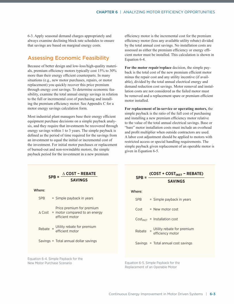
CHAPTER 6 | ANALYZING MOTOR EFFICIENCY OPPORTUNITIES
Continuous Energy Improvement in Motor Driven Systems | 6-3
6-3. Apply seasonal demand charges appropriately and always examine declining block rate schedules to ensure that savings are based on marginal energy costs.
Assessing Economic FeasibilityBecause of better design and low-loss/high-quality materi-als, premium efficiency motors typically cost 15% to 30% more than their energy efficient counterparts. In many situations (e.g., new motor purchases, repairs, or motor replacement) you quickly recover this price premium through energy cost savings. To determine economic fea-sibility, examine the total annual energy savings in relation to the full or incremental cost of purchasing and install-ing the premium efficiency motor. See Appendix C for a motor energy savings calculation form.
Most industrial plant managers base their energy efficient equipment purchase decisions on a simple payback analy-sis, and they require that investments be recovered through energy savings within 1 to 3 years. The simple payback is defined as the period of time required for the savings from an investment to equal the initial or incremental cost of the investment. For initial motor purchases or replacement of burned-out and non-rewindable motors, the simple payback period for the investment in a new premium
efficiency motor is the incremental cost for the premium efficiency motor (less any available utility rebate) divided by the total annual cost savings. No installation costs are assessed as either the premium efficiency or energy effi-cient motor must be installed. This calculation is shown in Equation 6-4.
For the motor repair/replace decision, the simple pay-back is the total cost of the new premium efficient motor minus the repair cost and any utility incentive (if avail-able), divided by the total annual electrical energy and demand reduction cost savings. Motor removal and instal-lation costs are not considered as the failed motor must be removed and a replacement spare or premium efficient motor installed.
For replacement of in-service or operating motors, the simple payback is the ratio of the full cost of purchasing and installing a new premium efficiency motor relative to the value of the total annual electrical savings. Base or “bare” motor installation costs must include an overhead and profit multiplier when outside contractors are used. A labor cost adjustment should be applied to motors with restricted access or special handling requirements. The simple payback given replacement of an operable motor is given in Equation 6-5.
SPB = ∆ COST − REBATE
SAVINGS
Where:
SPB = Simple payback in years
∆ Cost =Price premium for premium motor compared to an energy efficient motor
Rebate =Utility rebate for premium efficient motor
Savings = Total annual dollar savings
SPB = (COST + COSTINST − REBATE)
SAVINGS
Where:
SPB = Simple payback in years
Cost = New motor cost
CostINST = Installation cost
Rebate =Utility rebate for premium efficiency motor
Savings = Total annual cost savings
Equation 6-4. Simple Payback for the New Motor Purchase Scenario Equation 6-5. Simple Payback for the
Replacement of an Operable Motor

CHAPTER 6 | ANALYZING MOTOR EFFICIENCY OPPORTUNITIES
6-4 | Continuous Energy Improvement in Motor Driven Systems
The following analysis for purchasing a new 250-hp TEFC motor operating at 75% of full rated load illustrates how to use Equations 6-1 through 6-4. The analysis determines the cost effectiveness of purchasing a new premium efficiency motor having a 3/4-load efficiency of 96.2% (ηPREM = 96.2) instead of an energy efficient motor (ηEE = 95.5%). The motor is expected to be in operation for 8,000 hours per year. Electrical energy is purchased at a rate of $0.08/kWh with a demand charge of $8.00/kW/month.
Kilowatts saved (from Equation 6-1):
kWREDUCTION = 250 × 0.75 × 0.7457 × (100/95.5 − 100/96.2) = 1.06 kW
This is the amount of power conserved by the premium efficiency motor during each hour of use. Multiply this by the number of operating hours at the indicated load to obtain annual energy savings.
Energy saved (from Equation 6-2):
kWhSAVINGS = 1.06 × 8,000 = 8,480 kWh/year
Assuming utility energy and demand charges of $0.08/kWh and $8.00/kW/month (from Equation 6-3):
Cost Savings = (1.06 kW × 12 mo × $8.00/kW-mo) + (8,480 kWh/year × $0.08/kWh) = $780/year
In this example, installing a premium efficient motor reduces the utility bill by $780 per year. The simple payback for the incremental cost associated with a
premium efficiency motor purchase is the ratio of the price premium or incremental cost to total annual cost savings. Generally, premium efficiency motors might cost up to 15% to 30% more than a motor of an energy efficient design.
Assuming a price premium of $2,500 and no utility incentive, the simple payback on investment is as follows (from Equation 6-4):
SPB = ($2,500 – 0) / $780 = 3.2 years
The additional investment required to purchase a premium efficiency motor is recovered within 3.2 years. Premium efficiency motors often pay for themselves rapidly through reduced energy consumption and operating costs. After this initial payback period, annual savings will continue to be reflected in lower operating costs, and they will add to a company’s total profits.
Although the energy and cost savings associated with purchasing a premium efficiency motor can be impressive in many applications, selecting the premium efficiency unit is not always cost effective. Motors that are lightly loaded or infrequently used—such as motors driving control valves—may not consume enough electricity to allow the premium efficiency model to produce significant energy and cost savings. Remember, for a motor operating under a constant load, the electricity savings associated with an efficiency improvement are directly proportional to annual hours of operation. Special and definite purpose motors may carry a substantial price premium or may not be available in premium efficiency models.
Example 6-1

CHAPTER 6 | ANALYZING MOTOR EFFICIENCY OPPORTUNITIES
Continuous Energy Improvement in Motor Driven Systems | 6-5
References6-1 U.S. Department of Energy, Energy Efficient
Electric Motor Selection Handbook, DOE/GO-10095-290, August 1996.

Continuous Energy Improvement in Motor Driven Systems

CHAPTER 7 MOTOR EFFICIENCY IMPROVEMENT PLANNING

CHAPTER 7 | MOTOR EFFICIENCY IMPROVEMENT PLANNING
7-2 | Continuous Energy Improvement in Motor Driven Systems
An industrial facility should adopt a new motor pur-chase policy and plan ahead in order to implement energy efficiency measures when opportunities arise. Take the following planning steps for each motor in the plant that meets the minimum size requirements:
• Make field measurements necessary to determine actual motor loads.
• Establish the existing motor efficiency at its load point.
• Determine annual operating hours.
• Contact your utility account representative to determine if the utility offers a premium efficient motor rebate or has other energy efficiency incentive programs.
• Identify in-service standard efficiency motors that are cost-effective candidates for immediate replace-ment with a new premium efficient motor.
• Improve plant reliability and productivity through replacement of “problem” motors, i.e., those with a
history of frequent or repeated failures. Conduct fail-ure analyses to determine the root cause of the failure, correct system issues, and replace these motors with motor designs better suited for the application. With-out correcting the root cause of the failures, the reason for the continued failures may be passed along to the new premium efficient motor.
• Consider replacing motors that are less than 50% loaded with a downsized premium efficiency motor and a frame adapter.
• Consider the immediate replacement of older (pre-1964) U-frame motors with new premium efficiency T-frame motors.
• Conduct a repair/replace analysis to determine the cost-effectiveness of purchasing and installing new premium efficient motors versus rewinding or over-hauling failed standard efficiency motors.
• Establish a premium efficiency motor-ready spares inventory.
DOE has supported the development of MotorMaster+, a premium efficient motor selection and energy-management software tool.
MotorMaster+ software supports industrial energy management activities by providing the following:
■■ The ability to select the “best” available new or replacement motors using an internal database of price and performance information for more than 20,000 motors rated from 1 to 2,000 hp
■■ An in-plant motor inventory module in which motor nameplate data, operating hours and application information, and field measurements are linked to utility, facility, and process information
■■ The ability to automatically estimate in-service motor load and efficiency when field measurements are available
■■ The ability to scan for motors that operate under abnormal or sub-optimum power supply conditions
■■ Descriptor search capability to assist you in targeting energy-intensive equipment and replacing inefficient motors
■■ Inventory management functions, including maintenance logging and spares tracking
■■ Analysis features for rapidly determining the annual energy, demand, and dollar savings resulting from selecting and using a premium efficient motor in a new purchase or retrofit application
■■ The ability to conduct energy savings analyses for “batches” or selected populations of operating motors
■■ Energy accounting features, including summary reports on utility billing, plant production, energy efficiency measures installed, energy and dollar savings, and greenhouse gas emissions reductions
■■ Life-cycle costing capability, including the ability to compute the after-tax return on investment in energy efficiency measures.
In addition to MotorMaster+, the MotorMaster International software tool contains performance data for the 50 Hz IEC or metric motors in widespread use outside North America. It has all of MotorMaster+’s motor selection capabilities, including life-cycle costing. Both MotorMaster+ and MotorMaster International can be obtained at the AMO’s Energy Resource Center (www.eere.energy.gov/manufacturing/tech_assistance/ecenter.html).
MotorMaster+ Motor Energy Management Software

CHAPTER 7 | MOTOR EFFICIENCY IMPROVEMENT PLANNING
Continuous Energy Improvement in Motor Driven Systems | 7-3
• Consider the accelerated replacement of in-service standard efficiency motors.
• Prepare an action plan. Mark or tag motors so that the appropriate repair/replace action is taken at the time of motor failure.
Establish a New Motor Purchase PolicyEISA imposes mandatory minimum full-load efficiency standards for most general purpose motors in the 1- to 200-hp size range (see Chapter 4 for additional informa-tion). The result is that motors sold in or imported into the United States must already meet or exceed the premium efficiency motor performance standards. This requirement extends to foot-mounted motors with speeds of 3,600, 1,800, and 1,200 RPM and with ODP, TEFC, and explo-sion-proof enclosures.
EISA requires that general purpose motors with ratings between 201 and 500 hp must have a full-load efficiency that meets or exceeds the NEMA energy efficient motor standards. In addition, 1- to 200-hp U-frame, Design C, close-coupled pump, footless (C-face and D-flange), 900 RPM, vertical shaft normal-thrust, fire pump, and motors designed to operate on utilization voltages of 200 V and 575 V must also meet or exceed the energy efficient motor standards. While premium efficiency motors are available in most of these ratings, purchasing them is voluntary.
Consider a motor purchase policy that requires all new low and medium voltage motors in the 1- to 500-hp size range meet the NEMA premium efficiency motor stan-dards. Premium efficiency motors would be specified when ordering equipment from OEMs or for all imported equipment or process trains.
In-Service Motor Energy Efficiency OpportunitiesAn immediate motor replacement should be scheduled when your analysis indicates that replacing an operating motor with a premium efficiency model yields a simple payback period that meets your company investment criteria. Most of the time, the “triggering event” for an energy decision occurs when an operating motor fails and must be replaced. By planning ahead, you can develop an action plan and treat the motor failure as an opportunity to improve energy efficiency within your plant.
There are two basic scenarios that must be investigated. One assumes the failure of an operating motor; the second assumes there has been no motor failure. Each event calls for a different type of analysis. In each scenario, there are a number of alternatives to consider and analyze. The situ-ations and alternatives are as follows:
• The In-Service Motor Fails
- Repair the motor.
- Replace the motor with a new energy efficient motor (in ratings where they can still be sold).
- Replace the failed motor with a new premium effi-ciency motor.
• The In-Service Motor Does Not Fail
- Allow the motor to continue operating as is.
- Replace the motor immediately with a premium efficiency model.
In either situation, the alternatives can include downsizing if the existing motor is oversized and underloaded.
When an Operating Motor FailsWhen a motor fails, there are two options: repair the motor or replace it with a new one.
Repair the MotorFor larger motors, the least expensive approach in terms of capital costs is to repair the failed motor. Repair some-times means rewinding the stator in addition to making mechanical repairs and replacing bearings. The motor will, of course, be out of service during repairs. To justify a major rebuild, the original stator and rotor must be in serviceable or reasonably repairable condition. Repair of significant rotor or stator core damage usually is cost effective only on larger motors.
It is not unusual to find industries paying more to repair smaller general purpose standard efficiency motors than they would pay to purchase a new premium efficiency motor. Figure 7-1—prepared from actual cost quota-tions—shows that the repair cost (rewind plus bearing replacement) for motors 25 hp and below is about the same as the cost of a new premium efficiency severe duty motor. Taking into account its list price discount for the purchase of new premium efficiency motors, for this industrial facility, 1,800 RPM general purpose motors 25 hp and below should always be replaced when they require rewinding, regardless of their annual operating hours. Note that not all repairs require a motor rewind.

CHAPTER 7 | MOTOR EFFICIENCY IMPROVEMENT PLANNING
7-4 | Continuous Energy Improvement in Motor Driven Systems
Studies indicate that bearing failures account for approxi-mately two-thirds of all motor failures with winding fail-ures accounting for one-fifth of all failures.7-1
Even if a small operating premium efficiency motor were to fail, if it was not under warranty, it should be replaced with another premium efficiency motor instead of being repaired. Only repair the smaller special or definite pur-pose motors that have a significant price premium or are not available in a reasonable time frame. Premium effi-ciency motors generally cost about 15% to 30% more than standard efficiency motors.
Some industries determine a “horsepower breakpoint” that is used to establish and simplify their motor replace-ment policy. Motors larger than the breakpoint horsepower rating are typically rewound and returned to service when they fail; motors smaller than the breakpoint horsepower rating are recycled and replaced with new premium effi-ciency motors. Many process industries have established a horsepower breakpoint based upon cost-effectiveness at 50 hp.
The breakpoint horsepower for your plant is dependent on rewind costs, the list price discount your distributor applies to new premium efficiency motor purchases, utility rates and incentives, and annual operating hours for your motors. Appendix D contains a blank Motor Repair versus Replace Breakpoint worksheet. A completed worksheet provides the annual energy savings and simple payback periods from replacing failed standard efficiency motors
of various horsepower ratings with premium efficiency models. The simple payback lengthens as the horsepower rating increases. Scroll down to the highest horsepower rating where your simple payback criteria are satisfied. This is the horsepower breakpoint for your plant. A tool for determining the horsepower breakpoint is available on the Advanced Energy website (www.advancedenergy.org/portal/hp_breakpoint_tool/).
Industries typically cite simple paybacks in the range of 1 to 3 years for an energy efficiency project to be deemed as cost-effective. Reasons for lengthening the normal accept-able simple payback criteria for premium efficiency motor replacements include the secondary benefits associated with increasing both motor efficiency and durability—par-ticularly when the replacement motor is of severe-duty or IEEE 841 design. While difficult to quantify, these second-ary benefits occur due to the superior performance of the new premium efficiency motor in contrast to the perfor-mance of the rewound standard efficiency motor. The secondary benefits may include improved motor reliability and extended time between motor failures, warranty cov-erage if a motor does suffer an unexpected failure, and the potential for increased plant up-time accompanied by an increase in production.
Replace the Failed Motor with a New Premium Efficiency Model When replacement is needed, it is often cost effective to purchase a new premium efficient motor. Exceptions can include when an energy efficient motor is in the spares
Horsepower
1,800 RPM — Repair Versus New Motor Cost
Cost
$4,000
$3,500
$3,000
$2,500
$2,000
$1,500
$1,000
$500
$05 7.5 10 20 25 30 40 50 60 7515
Repair Cost
Premium Motor Cost
Figure 7-1. Repair and New Premium Efficiency Motor Costs (for 1,800 RPM TEFC Motors, 2011 Prices)

CHAPTER 7 | MOTOR EFFICIENCY IMPROVEMENT PLANNING
Continuous Energy Improvement in Motor Driven Systems | 7-5
inventory or annual operating hours that are very low, or both. When a previously rewound standard efficient motor fails, however, it should always be considered for replace-ment with a premium efficient motor.
The economic analysis for deciding whether to repair or replace a failed motor is straightforward. The “do nothing” alternative doesn’t apply. The least-capital-cost alterna-tive, overhauling (bearing replacement plus clean, dip, and bake) or rewinding and installing new bearings on the failed motor becomes the base case. The biggest chal-lenge is estimating the cost of the repair and the motor’s efficiency after repair. MotorMaster+ can be of help as it provides default motor repair costs (rewind plus bearings) plus default losses that might be incurred during the motor repair process if repair best practices are not followed.
Start your analysis by identifying the operating cost of each alternative action. It is then possible to compare both the incremental cost of the alternative and the operat-ing cost reduction associated with it. Energy consumed in motor losses is given in terms of kWh. Differences in operating costs are easy to compute using information from the utility rate schedule. Always use marginal or incremental energy and capacity costs.
Results of a MotorMaster+ “repair versus replace” analy-sis are summarized in Table 7-1. Comparative perfor-mance values are based on an energy cost of $0.08/kWh and a monthly demand charge of $8.00/kW/month. You can also calculate these values with the equations pro-vided in Chapter 6. Absent utility incentives, the analysis indicates a 2.5 year simple payback on the investment in a premium efficiency replacement motor. The failed motor could be rewound and retained as a spare, recycled, or sold for its salvage value.
The MotorMaster+ compare module allows for a side-by-side comparison of motors with different horsepower ratings. It can even adjust the output power for part-load operating speed differences for motor-driven “affinity law” loads (e.g., centrifugal pumps or fans).
You will have to weigh several factors to make a good repair versus replace decision:
• Cost of the replacement premium efficiency motor
• Efficiency of proposed premium efficiency motor
• Downtime cost for each alternative (if different)
• Cost to overhaul or rewind the existing motor
• Efficiency of the existing motor after repair
• Availability of a utility rebate.
Table 7-1. Motor Rewind Versus Replacement Analysis (100 hp, 1,800 RPM, TEFC Motor)
Repaired Standard Efficiency
Motor
New Premium Efficiency
Motor
Motor Rating (hp) 100 100
Load, % 75 75
Efficiency at Load Point, % 92.2 95.3
Motor Rewind Loss, % 0.51 ---
Annual Operating Hours 6,000 6,000
Cost (Rewind/Purchase) $2,590 $5,9402
Motor Rebate (None)
Annual Energy Use, kWh 366,002 352,256
Annual Energy Cost, $ $29,280 $28,180
Demand Charge, ($/year) $5,856 $5,636
Savings Compared to Repair
Energy (kWh/year) 13,746
Energy Value ($/year) $1,100
Demand Reduction (kW) 2.3
Demand Savings ($/year) $220
Total Savings ($/year) $1320
Simple Payback (years) 2.5
1 If repair best practices are followed, no efficiency loss reduction should be expected.
2Assumes a 50% list price discount.
CHAPTER 7 | MOTOR EFFICIENCY IMPROVEMENT PLANNING
7-6 | Continuous Energy Improvement in Motor Driven Systems
Information on premium efficiency motor costs and efficiency at various load points is available from Motor-Master+, the motor manufacturer, or your local motor distributor. Downtime costs are often the same for each alternative. In general, large or special-purpose motors can be repaired more quickly than they can be replaced, but distributors usually have premium efficiency general purpose motors in stock or can quickly obtain them from a motor manufacturer’s regional warehouse.
The motor comparison window of MotorMaster+ pro-vides a default cost for repair (rewind plus new bearings) for your existing motor, but it can be overwritten. In fact, it usually needs to be overwritten, because motor repair costs vary too much for users to rely on the default num-ber for investment decisions. Repair costs vary with the extent of damage, geographical location, overtime require-ments, and type of stator impregnation. Moreover, repairs are usually done by companies or shops rather than by manufacturers, so there is no annual update of repair costs in the MotorMaster+ database. You can obtain better infor-mation on repair costs in one of two ways. You can main-tain your own cost database using records of recent repairs or request a price list from your local service center. Alter-natively, you can subscribe to a motor repair cost guide that is updated annually. A widely used price estimator is available from Vaughens’ Price Publishing Company.7-2
Motor rewind losses may range from a 0.50% to 1% effi-ciency reduction for 40 hp or smaller motors and 0.25% to 0.50% for motors over 40 hp if repair best practices are not followed.7-4 If good repair practices are followed, no reduc-tion in efficiency should be expected. Require that your service center adheres to the repair practices recommended in ANSI/EASA Standard AR100-2010.7-3 Large industries maintain staff that regularly audit their motor service cen-ters. Look for evidence of a quality management program such as Proven Efficiency Verification (www.advanceden-ergy.org/programs/proven-efficiency-verification-for-motor-repair), the Green Motors Practices Group (www.greenmo-tors.org/gmi.htm), ISO 9000, or EASA-Q.
When an Existing Motor Does Not FailIf the monitor continues to function, the energy manager has two options: let the motor operate as usual or replace it with a new premium efficiency one.
Let the Motor Continue to Operate As IsThere are many demands on an energy manager’s time; thus, reducing motor losses may not be a high priority in comparison to other important duties. In addition, there are no immediate costs associated with keeping a working standard efficiency motor operating. Savings may simply accrue too slowly to justify the investment in a new pre-mium efficiency motor. Each plant is different, so deci-sions concerning the relative importance of projects are best left to those responsible for operating the plant.
Replace Operating Motor with a New Premium Efficiency MotorA premium efficiency replacement motor can often be found in the same frame size as an existing standard effi-ciency T-frame motor, and with comparable starting torque and locked-rotor current. Frame adapters or conversion bases are necessary for pre-1952 motors, U-frame motors, and special designs. The average premium efficiency motor rotates at a fraction of a percent higher speed than its standard efficiency counterpart. In many centrifugal pump and fan applications, this will increase flow and energy consumption, which can offset or diminish the expected energy savings. Full-load speeds do vary among premium efficiency motors, and a model can often be found to closely match the speed of all but the slowest standard efficiency motors. You can change sheave or pul-ley sizes with belt-driven loads so the rotating equipment operates at its original or required speed. An increase in replacement motor full-load speed is not of importance when the motor is controlled by a variable speed drive.
Table 7-2 illustrates the benefits of replacing an exist-ing in-service standard efficiency motor with a premium efficiency model (again, new motor price and performance information comes from MotorMaster+). Comparative performance values are based on an energy cost of $0.08/kWh and a monthly demand charge of $8/kW/month.
Replacing an operating motor is usually not cost effective. The 5.1-year simple payback in the example shown in Table 7-2 is much longer than the simple payback accept-able to most industrial plant managers. Payback, however, is very sensitive to individual circumstances. An operating time of 8,000 hours or availability of a utility rebate would reduce the simple payback period, and higher electrical energy and demand costs would reduce it even further.
Helpful Tip
For more information on the repair process, see the 2003 EASA/AEMT Rewind Study7-4 The Effect of Repair/Rewinding on Motor Efficiency and DOE’s Model Repair Specifications for Low Voltage Induction Motors available at the AMO’s Energy Resource Center (www.eere.energy.gov/manufacturing/tech_assistance/ecenter.html).
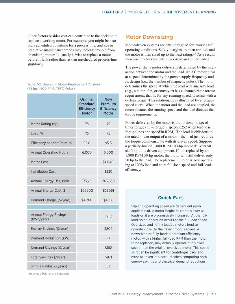
CHAPTER 7 | MOTOR EFFICIENCY IMPROVEMENT PLANNING
Continuous Energy Improvement in Motor Driven Systems | 7-7
Other factors besides cost can contribute to the decision to replace a working motor. For example, you might be near-ing a scheduled downtime for a process line, and age or predictive maintenance trends may indicate trouble from an existing motor. It usually is wise to replace a motor before it fails rather than risk an unscheduled process-line shutdown.
Motor DownsizingMotor-driven systems are often designed for “worst case” operating conditions. Safety margins are then applied, and the motor is then sized up to the next rating.7-5 As a result, in-service motors are often oversized and underloaded.
The power that a motor delivers is determined by the inter-action between the motor and the load. An AC motor turns at a speed determined by the power supply frequency and its design (i.e., the number of magnetic poles). The motor determines the speed at which the load will run. Any load (e.g., a pump, fan, or conveyor) has a characteristic torque requirement; that is, for any running speed, it resists with a certain torque. This relationship is illustrated by a torque-speed curve. When the motor and the load are coupled, the motor dictates the running speed and the load dictates the torque requirements.
Power delivered by the motor is proportional to speed times torque (hp = torque × speed/5,252 when torque is in foot-pounds and speed in RPM). The load is oblivious to the rated power output of a motor—the load just requires the torque commensurate with its driven speed. Suppose a partially-loaded 1,800 RPM 100-hp motor delivers 50 shaft hp to its driven equipment. If it is replaced by an 1,800 RPM 50-hp motor, the motor will still deliver only 50 hp to the load. The replacement motor is now operat-ing at 100% load and at its full-load speed and full-load efficiency.
Table 7-2. Operating Motor Replacement Analysis (75 hp, 1,800 RPM, TEFC Motor)
Original Standard Efficiency
Motor
New Premium Efficiency
Motor
Motor Rating (hp) 75 75
Load, % 75 75
Efficiency at Load Point, % 92.0 95.5
Annual Operating Hours 6,000 6,000
Motor Cost $4,6401
Installation Cost $330
Annual Energy Use, kWh 273,751 263,639
Annual Energy Cost, $ $21,900 $21,091
Demand Charge, ($/year) $4,380 $4,218
Annual Energy Savings (kWh/year)
10,112
Energy Savings ($/year) $809
Demand Reduction (kW) 1.7
Demand Savings ($/year) $162
Total Savings ($/year) $971
Simple Payback (years) 5.1
1Assumes a 50% list price discount.
Quick Fact
Slip and operating speed are dependent upon applied load. A motor begins to rotate slower as loads on it are progressively increased. At the full-load point, operation occurs at the full-load speed. Oversized and lightly loaded motors tend to operate closer to their synchronous speed. A downsized or fully-loaded premium efficiency motor, with a higher full-load RPM than the motor to be replaced, may actually operate at a slower speed than the original oversized motor. This speed shift can be significant for centrifugal loads and must be taken into account when computing both energy savings and electrical demand reductions.

CHAPTER 7 | MOTOR EFFICIENCY IMPROVEMENT PLANNING
7-8 | Continuous Energy Improvement in Motor Driven Systems
Downsizing can be a money-saver for two reasons:
• When purchasing replacement motors, smaller motors tend to cost less.
• An under-loaded motor operates less efficiently and with lower power factor than a motor loaded at 75% to 100% of rated power.
Motor efficiency curves vary by horsepower rating and synchronous speed, but most peak near 75% load and still provide near-nameplate efficiency at half-load. Below half-load, efficiency begins to drop off dramatically. Performance curves for two typical motors are presented in Figure 7-2. When determining energy savings due to replacing an in-service motor with a downsized model, you must determine the appropriate part-load efficiency for each motor. Since larger motors exhibit a higher effi-ciency over their load range, it is possible to find that the larger standard efficiency motor’s half-load efficiency is comparable to or greater than the full-load efficiency of a premium efficiency replacement motor rated at half the power output.7-6
Table 7-3 summarizes the energy savings from replac-ing an in-service 40%-loaded 100-hp motor with down-sized standard and premium efficiency motors of differ-ent horsepower ratings. The table shows the efficiency at the load point given that motors of different horsepower ratings and efficiency classes are used to satisfy the fixed 40-hp load. The analysis takes into account the motor efficiency at the load point and indicates the input power requirements (kW) for all of the replacement motor choices.
When the 100-hp standard efficiency motor is replaced with a 40-hp standard efficiency motor, the result is only a 0.37 kW reduction in input power (33.45 kW – 33.08 kW).
Table 7-3. Motor Downsizing Versus Efficiency Class of Replacement Motor. Source: WSU Motor Training Materials
Motor Rating, hp
Motor Oversizing 40% Load on a 100 Horsepower Motor
Standard Efficiency Premium Efficiency
Efficiency at Load Point, % Input kW Efficiency at Load Point, % Input kW
100 89.2 33.45 93.7 31.84
75 91.1 32.75 95.1 31.37
60 91.5 32.60 94.9 31.44
50 91.6 32.57 94.8 31.47
40 90.2 33.08 94.2 31.67
Percent of Full Load
Perc
ent E
�ci
ency
and
Pow
er F
acto
r
25 50 75 10040
50
60
70
80
90
100
25 hp power factor
100 hp power factor
25 hp e�ciency
100 hp e�ciency
Figure 7-2. Motor Performance at Part-Load. Illustration from EM4MDS
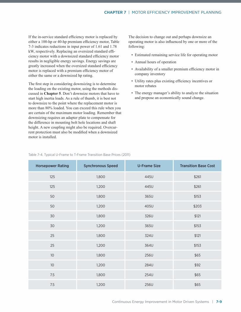
CHAPTER 7 | MOTOR EFFICIENCY IMPROVEMENT PLANNING
Continuous Energy Improvement in Motor Driven Systems | 7-9
If the in-service standard efficiency motor is replaced by either a 100-hp or 40-hp premium efficiency motor, Table 7-3 indicates reductions in input power of 1.61 and 1.78 kW, respectively. Replacing an oversized standard effi-ciency motor with a downsized standard efficiency motor results in negligible energy savings. Energy savings are greatly increased when the oversized standard efficiency motor is replaced with a premium efficiency motor of either the same or a downsized hp rating.
The first step in considering downsizing is to determine the loading on the existing motor, using the methods dis-cussed in Chapter 5. Don’t downsize motors that have to start high inertia loads. As a rule of thumb, it is best not to downsize to the point where the replacement motor is more than 80% loaded. You can exceed this rule when you are certain of the maximum motor loading. Remember that downsizing requires an adapter plate to compensate for the difference in mounting bolt hole locations and shaft height. A new coupling might also be required. Overcur-rent protection must also be modified when a downsized motor is installed.
The decision to change out and perhaps downsize an operating motor is also influenced by one or more of the following:
• Estimated remaining service life for operating motor
• Annual hours of operation
• Availability of a smaller premium efficiency motor in company inventory
• Utility rates plus existing efficiency incentives or motor rebates
• The energy manager’s ability to analyze the situation and propose an economically sound change.
Table 7-4. Typical U-Frame to T-Frame Transition Base Prices (2011)
Horsepower Rating Synchronous Speed U-Frame Size Transition Base Cost
125 1,800 445U $261
125 1,200 445U $261
50 1,800 365U $153
50 1,200 405U $203
30 1,800 326U $121
30 1,200 365U $153
25 1,800 324U $121
25 1,200 364U $153
10 1,800 256U $65
10 1,200 284U $92
7.5 1,800 254U $65
7.5 1,200 256U $65
CHAPTER 7 | MOTOR EFFICIENCY IMPROVEMENT PLANNING
7-10 | Continuous Energy Improvement in Motor Driven Systems
Upgrade Old U-Frame to Premium Efficiency T-Frame MotorsConsider immediately replacing in-service standard effi-cient U-frame motors with premium efficiency T-frame motors. U-frame motors were the industry standard between 1952 and 1964. Eliminating old U-frame motors simplifies the spares inventory as only T-frame motors need to be stocked in the spares warehouse. Although pre-mium efficiency U-frame motors are available from motor manufacturers (they are often referred to as “automotive duty” motors), they carry a significant price premium; in fact, for 10-hp and 15-hp 1,800 RPM motors, the cost for a new U-frame motor is more than double the cost of an equivalent premium efficiency motor of a T-frame design.
A U-frame to T-frame conversion requires a frame adapter or transition base to line up mounting bolt holes on the base and to provide the correct shaft height. While pur-chase of a transition base does incur an additional motor replacement cost, this cost is offset by the typical 15% U-frame price adder to the base price for repair of a stan-dard efficiency T-frame motor.7-2 Transition base prices are given in Table 7-4.7-7
Since no repair or replacement is required, the simple payback for a U-frame motor replacement should include the full cost of purchasing and installing the premium efficiency T-frame motor plus a frame adapter, divided by the annual energy cost savings. Maintenance and plant reliability benefits will also be realized if condition assess-ment tests indicate that the U-frame motor is expected to fail in the near future.
Establish a Premium Efficiency-Ready Spares InventoryA PEM-Ready spares inventory is established by identify-ing motor ratings and frame sizes where a number of stan-dard efficiency motors are in operation and no premium efficiency spare is available in the event of a standard efficiency motor failure. Purchasing a block of premium efficiency motors to store in the on-site spares warehouse should ensure that a premium efficiency motor is installed when any standard efficiency or energy efficient motor fails. A failed standard efficiency motor should be recycled and a new premium efficiency motor purchased to replace the premium efficiency motor that was installed. Failed energy efficient and premium efficiency motors would be repaired and returned to the spares warehouse unless the repair cost exceeds the cost of a new premium efficiency motor. With this process, the PEM-Ready spare inven-tory automatically replenishes itself. The ultimate goal is to remove existing standard efficiency motors from the spares inventory so they cannot be returned to service when a standard efficiency motor fails.
A PEM-Ready spares inventory is only necessary when replacement premium efficiency motors are not imme-diately available from the local distributor. Depending on their size, the distributor usually has general purpose motors up to 50 hp or 100 hp in their warehouse and
Helpful Tip
If the old U-frame motors are not immediately replaced with premium efficient T-frame motors, purchase and maintain an inventory of U- to T-frame adapters or conversion bases. Without ready access to a conversion base, an old standard efficiency U-frame motor from the spares inventory is likely to be installed with the failed U-frame motor rewound and placed into the spares inventory.
Quick Fact
Unless you have a PEM-Ready spares inventory or immediate access to new premium efficiency motors from your motor distributor, a delay can occur before you can begin to capture the energy and operating cost savings expected through modifying repair/replace practices. The delay occurs because, upon the failure of an operating standard efficiency motor, a standard efficiency motor from the spares inventory would be installed whenever a premium efficiency motor was not immediately available. The failed motor would be recycled, and a new premium efficiency motor ordered as a replacement. When the premium efficiency motor arrives at the plant, it would be held in the spares inventory until the next failure of a standard efficiency motor. In the worst case scenario, the failed standard efficiency motor would be repaired and returned to service, which would eliminate the opportunity for energy and operating cost savings.
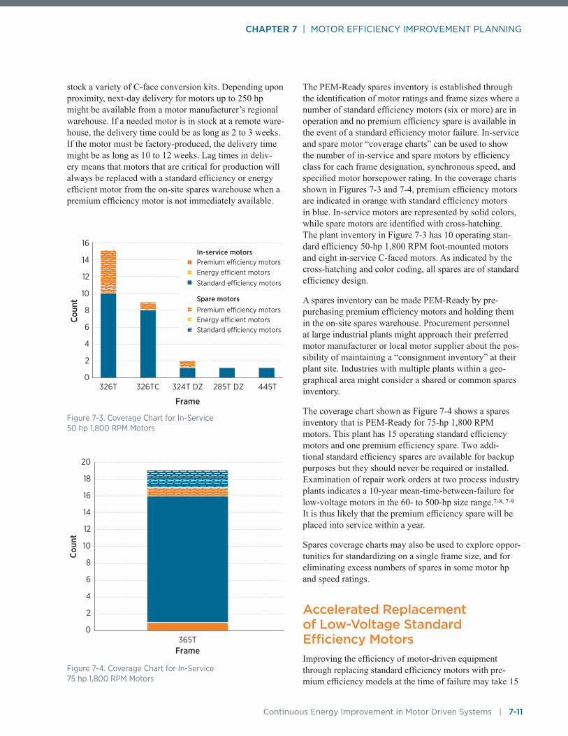
CHAPTER 7 | MOTOR EFFICIENCY IMPROVEMENT PLANNING
Continuous Energy Improvement in Motor Driven Systems | 7-11
stock a variety of C-face conversion kits. Depending upon proximity, next-day delivery for motors up to 250 hp might be available from a motor manufacturer’s regional warehouse. If a needed motor is in stock at a remote ware-house, the delivery time could be as long as 2 to 3 weeks. If the motor must be factory-produced, the delivery time might be as long as 10 to 12 weeks. Lag times in deliv-ery means that motors that are critical for production will always be replaced with a standard efficiency or energy efficient motor from the on-site spares warehouse when a premium efficiency motor is not immediately available.
The PEM-Ready spares inventory is established through the identification of motor ratings and frame sizes where a number of standard efficiency motors (six or more) are in operation and no premium efficiency spare is available in the event of a standard efficiency motor failure. In-service and spare motor “coverage charts” can be used to show the number of in-service and spare motors by efficiency class for each frame designation, synchronous speed, and specified motor horsepower rating. In the coverage charts shown in Figures 7-3 and 7-4, premium efficiency motors are indicated in orange with standard efficiency motors in blue. In-service motors are represented by solid colors, while spare motors are identified with cross-hatching. The plant inventory in Figure 7-3 has 10 operating stan-dard efficiency 50-hp 1,800 RPM foot-mounted motors and eight in-service C-faced motors. As indicated by the cross-hatching and color coding, all spares are of standard efficiency design.
A spares inventory can be made PEM-Ready by pre-purchasing premium efficiency motors and holding them in the on-site spares warehouse. Procurement personnel at large industrial plants might approach their preferred motor manufacturer or local motor supplier about the pos-sibility of maintaining a “consignment inventory” at their plant site. Industries with multiple plants within a geo-graphical area might consider a shared or common spares inventory.
The coverage chart shown as Figure 7-4 shows a spares inventory that is PEM-Ready for 75-hp 1,800 RPM motors. This plant has 15 operating standard efficiency motors and one premium efficiency spare. Two addi-tional standard efficiency spares are available for backup purposes but they should never be required or installed. Examination of repair work orders at two process industry plants indicates a 10-year mean-time-between-failure for low-voltage motors in the 60- to 500-hp size range.7-8, 7-9 It is thus likely that the premium efficiency spare will be placed into service within a year.
Spares coverage charts may also be used to explore oppor-tunities for standardizing on a single frame size, and for eliminating excess numbers of spares in some motor hp and speed ratings.
Accelerated Replacement of Low-Voltage Standard Efficiency MotorsImproving the efficiency of motor-driven equipment through replacing standard efficiency motors with pre-mium efficiency models at the time of failure may take 15
Coun
t
Frame
16
14
12
10
8
6
4
2
0326T 326TC 324T DZ 285T DZ 445T
In-service motors
Spare motors
Standard e�ciency motorsEnergy e�cient motorsPremium e�ciency motors
Standard e�ciency motorsEnergy e�cient motorsPremium e�ciency motors
Coun
t
Frame
20
18
16
14
12
10
8
6
4
2
0365T
Figure 7-3. Coverage Chart for In-Service 50 hp 1,800 RPM Motors
Figure 7-4. Coverage Chart for In-Service 75 hp 1,800 RPM Motors
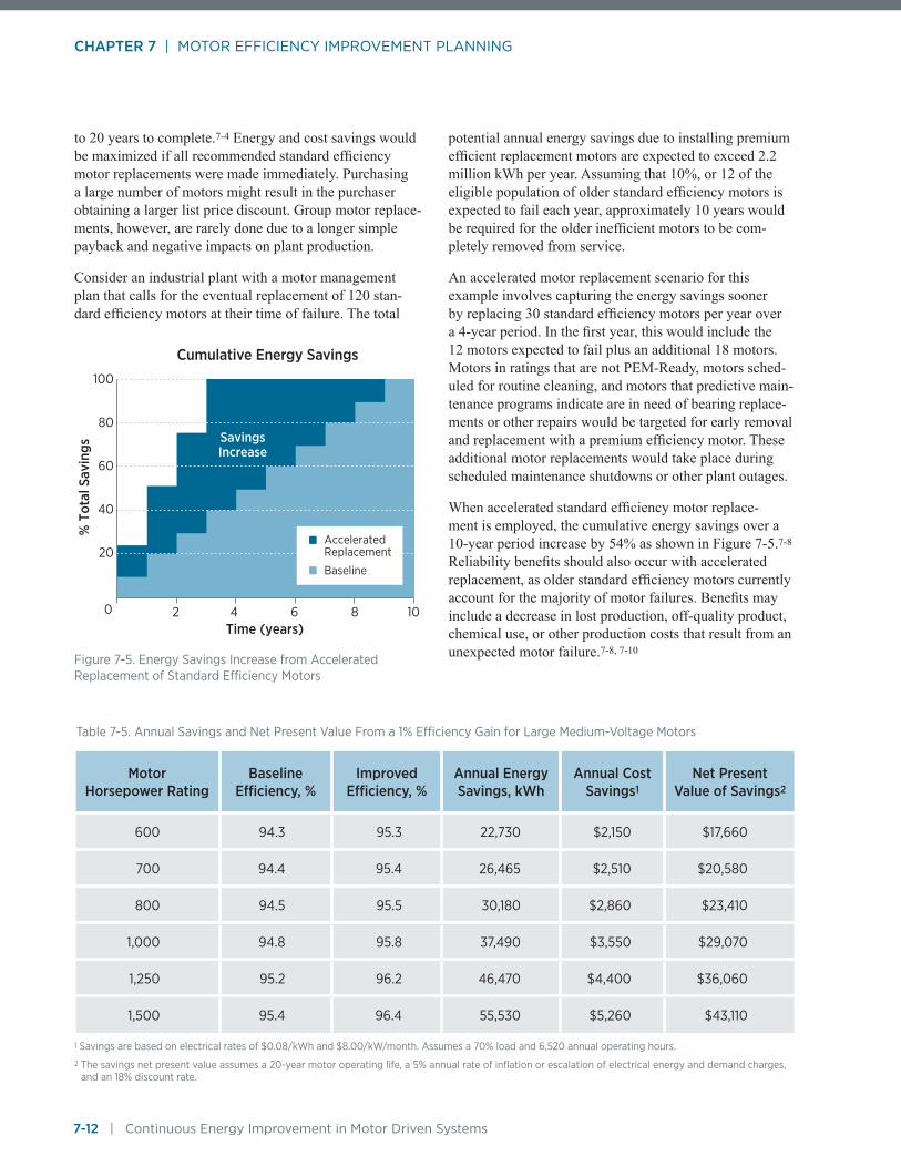
CHAPTER 7 | MOTOR EFFICIENCY IMPROVEMENT PLANNING
7-12 | Continuous Energy Improvement in Motor Driven Systems
to 20 years to complete.7-4 Energy and cost savings would be maximized if all recommended standard efficiency motor replacements were made immediately. Purchasing a large number of motors might result in the purchaser obtaining a larger list price discount. Group motor replace-ments, however, are rarely done due to a longer simple payback and negative impacts on plant production.
Consider an industrial plant with a motor management plan that calls for the eventual replacement of 120 stan-dard efficiency motors at their time of failure. The total
potential annual energy savings due to installing premium efficient replacement motors are expected to exceed 2.2 million kWh per year. Assuming that 10%, or 12 of the eligible population of older standard efficiency motors is expected to fail each year, approximately 10 years would be required for the older inefficient motors to be com-pletely removed from service.
An accelerated motor replacement scenario for this example involves capturing the energy savings sooner by replacing 30 standard efficiency motors per year over a 4-year period. In the first year, this would include the 12 motors expected to fail plus an additional 18 motors. Motors in ratings that are not PEM-Ready, motors sched-uled for routine cleaning, and motors that predictive main-tenance programs indicate are in need of bearing replace-ments or other repairs would be targeted for early removal and replacement with a premium efficiency motor. These additional motor replacements would take place during scheduled maintenance shutdowns or other plant outages.
When accelerated standard efficiency motor replace-ment is employed, the cumulative energy savings over a 10-year period increase by 54% as shown in Figure 7-5.7-8 Reliability benefits should also occur with accelerated replacement, as older standard efficiency motors currently account for the majority of motor failures. Benefits may include a decrease in lost production, off-quality product, chemical use, or other production costs that result from an unexpected motor failure.7-8, 7-10
% T
otal
Sav
ings
Time (years)
100
80
60
40
20
Cumulative Energy Savings
20 4 6 8 10
Accelerated Replacement
Baseline
SavingsIncrease
Figure 7-5. Energy Savings Increase from Accelerated Replacement of Standard Efficiency Motors
Table 7-5. Annual Savings and Net Present Value From a 1% Efficiency Gain for Large Medium-Voltage Motors
Motor Horsepower Rating
Baseline Efficiency, %
Improved Efficiency, %
Annual Energy Savings, kWh
Annual Cost Savings1
Net Present Value of Savings2
600 94.3 95.3 22,730 $2,150 $17,660
700 94.4 95.4 26,465 $2,510 $20,580
800 94.5 95.5 30,180 $2,860 $23,410
1,000 94.8 95.8 37,490 $3,550 $29,070
1,250 95.2 96.2 46,470 $4,400 $36,060
1,500 95.4 96.4 55,530 $5,260 $43,110
1 Savings are based on electrical rates of $0.08/kWh and $8.00/kW/month. Assumes a 70% load and 6,520 annual operating hours.
2 The savings net present value assumes a 20-year motor operating life, a 5% annual rate of inflation or escalation of electrical energy and demand charges, and an 18% discount rate.

CHAPTER 7 | MOTOR EFFICIENCY IMPROVEMENT PLANNING
Continuous Energy Improvement in Motor Driven Systems | 7-13
Improve the Efficiency of your Medium-Voltage MotorsNo mandatory minimum full-load efficiency standards exist for motors rated above 500-hp. While manufactur-ers may market motors exceeding 500 hp as “energy efficient,” “high efficiency,” or “premium efficiency,” these terms historically had no common definitions for either low or medium voltage motors One manufacturer’s “standard efficiency” motor may be found to have a higher full-load efficiency than another manufacturer’s in-service “premium efficiency” motor model. Plant staff indicate that large medium voltage motors are mainly purchased based on availability and matching frame size—not on energy efficiency.
Medium voltage motor manufacturers can often offer price quotations for a “standard” and an “improved efficiency” product. The annual energy and cost savings benefit due to a 1% gain in operating efficiency for large medium volt-age motors is shown in Table 7-5 for a given set of electric rates and other assumptions. The baseline efficiency values have been recommended for use by Pacific Gas & Electric (PG&E) for their incentive programs.
The net present value of a stream of uniform energy sav-ings can be obtained using life cycle costing techniques, such as those available in the MotorMaster+ software tool. Table 7-5 indicates that a 1% efficiency improvement on an 800-hp motor would provide an annual energy sav-ings of more than 30,180 kWh valued at $2,150 annually for the example electric rates. The net present value of these savings is equal to $23,410 for the listed assump-tions. This means that the purchaser of an 800-hp motor should be willing to pay a price premium of up to $23,410 to obtain a single point of efficiency improve-ment. All results are based upon a motor load of 70% with 6,520 hours of operation annually. Net present val-ues given a 1% motor efficiency improvement for other medium voltage motor horsepower ratings are given in Table 7-5. Note that net present values are extremely sen-sitive to changes in future electrical energy rates and the selected discount rate. The net present values shown do not include benefits due to potentially available equipment tax credits or accelerated depreciation.
Examine Motor Repair PracticesRequest that your local service center repair all motors in accordance with ANSI/EASA AR100-2010 repair best practices.7-3 The selected service center should have a phi-losophy of repairing any failed motor to its original design through use of EASA guidelines. They should maintain a large stock of inverter-grade magnet wire in various wire gauges so they can install the correct wire size and replicate the original number of turns in a motor’s wind-ing pattern. A pre-repair core loss test should be conducted to determine the motor’s suitability for repair. Replace-ment may be required if core steel is damaged from the motor failure or from previous repairs. The service center should hold their reclaiming oven temperature to 700°F to prevent core damage and always perform a post-repair core loss test.
The selected repair shop should provide a detailed “general test report” and stator “core loss test report” when a failed motor is repaired and returned to the spares warehouse. The core loss pre- and post-repair tests are desirable, as they provide the core dimensions, identify hot spots with recommendations, provide core loss test setup information, and show metered data including the core loss in watts/pound. The measured value is put into perspective by comparing it against a maximum allowable limit. Differ-ences in watts per pound before and after repair may also indicate quality issues in the repair process.
Figure 7-6. Sample In-Service Motor Repair/Replace Tags. Tags from Advanced Energy
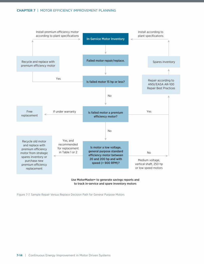
CHAPTER 7 | MOTOR EFFICIENCY IMPROVEMENT PLANNING
7-14 | Continuous Energy Improvement in Motor Driven Systems
Install premium e�ciency motor according to plant specifications
Yes
If under warranty Yes
No
No
No
Medium voltage, vertical shaft, 250 hp or low speed motors
Yes, andrecommended
for replacement in Table 1 or 2
Install according to plant specifications
Free replacement
Recycle old motor and replace with
premium e�ciency motor from strategic spares inventory or
purchase new premium e�ciency
replacement
Use MotorMaster+ to generate savings reports and to track in-service and spare inventory motors
Is failed motor a premium e�ciency motor?
Is motor a low voltage, general purpose standard e�ciency motor between 20 and 200 hp and with
speed (> 900 RPM)?
Recycle and replace with premium e�ciency motor
Failed motor repair/replace.
Is failed motor 15 hp or less? Repair according to ANSI/EASA AR-100
Repair Best Practices
Spares inventory
In-Service Motor Inventory
Figure 7-7. Sample Repair Versus Replace Decision Path for General Purpose Motors

CHAPTER 7 | MOTOR EFFICIENCY IMPROVEMENT PLANNING
Continuous Energy Improvement in Motor Driven Systems | 7-15
A typical general test report might contain comments relat-ing to the cause of the motor failure, nameplate data, elec-trical test results (insulation to ground, hipot test, surge test, phase-to-phase resistance, and a no-load test with volts and amps for each phase), mechanical data including grease type and amount of endplay, temperature readings, and vibration test results (displacement and velocity in the horizontal, vertical, and axial directions for both the drive end and opposite drive end bearings).
Prepare an Action PlanThe action plan should contain a list of recommendations from the motor management plan along with required future actions, the designation of an individual responsible for carrying out those actions, and a completion date.
The motor management plan contains recommendations regarding repair or replacement for each in-service motor. The plan might also recommend investigating the cost-effectiveness of retrofitting adjustable speed control onto motors driving pumps that use throttling valves or recircu-lation lines to provide flow control or with fans that oper-ate with partially closed inlet or discharge dampers. Of particular importance is the “tagging” of these motors. All motors should be tagged so millwrights and maintenance staff can take the appropriate action(s) when an in-service motor fails. Sample motor tags developed by Advanced Energy are depicted in Figure 7-6. Tag durability is of importance. Note that these tags are fastened to the motors with metal reinforced rings and are coated in plastic to protect against moisture and grease.
It is also of use to prepare a flow chart that depicts the adopted repair versus replace practice. A sample post-motor management plan repair versus replace decision-making path is shown in Figure 7-7. Lastly, plant staff should continue to use MotorMaster+ or a comparable software tool for inventory management, maintenance logging, warranty tracking, and energy savings reporting activities.
Continuous Energy Improvement in Motor Driven Systems
References 7-1 Bonnett, Austin H. and Chuck Yung, “A Construc-
tion, Performance and Reliability Comparison for Pre-EPCA, EPCA and Premium-Efficient Motors,” IEEE Paper No. PCIC-2006-7, 2006.
7-2 2011 Pocket Pricing Pal: 2011 USA National Average Prices for Repair of AC and DC Motors, Vaughen’s Price Publishing Co. Inc., 2011.
7-3 Electrical Apparatus Service Association, Inc., ANSI/EASA AR100-2010: Recommended Practice for the Repair of Rotating Electrical Apparatus, October 2010.
7-4 Electrical Apparatus Service Association, Inc., The Effect of Repair/Rewinding on Motor Effi-ciency: EASA/AEMT Rewind Study and Good Practice Guide, 2003.
7-5 Malinowski, John, Baldor Electric Company, Electrical Efficiency: Spec the Right Motor and Drive for Lifecycle Performance, November, 2011.
7-6 Nailen, Richard L., “Bigger Might be Better,” Electrical Apparatus, March 1997.
7-7 McCoy, Gilbert A, Washington State University Energy Program, Motor Management Plan for Blue Ridge Fiberboard, prepared for the GenEDGE Alliance and Blue Ridge Fiberboard, October 2011.
7-8 McCoy, Gilbert A, and Johnny Douglass, Washing-ton State University Energy Program, Motor Management Plan for the Domtar Kamloops Pulp Mill, prepared for BC Hydro, December, 2007.
7-9 McCoy, Gilbert A., Washington State University Energy Program, Motor Management Plan for the Quesnel River Pulp Mill, prepared for BC Hydro, April 2008.
7-10 McCoy, Gilbert A., “Beyond Minimum Energy Performance Standards (MEPS): Getting Premium Efficiency Motors Installed in Your Plant,” pre-sented at the Energy Efficiency in Motor Driven Systems Conference, Nantes, France, September 2009.

CHAPTER 8 SYSTEM EFFICIENCY IMPROVEMENT OPPORTUNITIES

CHAPTER 8 | SYSTEM EFFICIENCY IMPROVEMENT OPPORTUNITIES
8-2 | Continuous Energy Improvement in Motor Driven Systems
While motor efficiency is certainly of importance, it is a relatively small contributor to overall system efficiency. System efficiency is the efficiency of converting electrical input energy into useful mechanical work. It is the useful energy output divided by the energy input. Those doing energy assessments of pumping systems might speak of the efficiency of a single component such as the motor or pump while determining the “wire-to-water” pump-ing plant efficiency. The wire-to-water efficiency of your pumping plant is the water horsepower provided by your pumping plant—which is proportional to the delivered fluid flow (in gallons per minute [gpm]) times the static head produced by the pump (in feet)—divided by the elec-trical input power supplied to the pump drive motor. The greater your overall wire-to-water or system efficiency, the lower your overall pumping costs will be.
A system can be comprised of much more than just a motor, power transmission system, and a pump. The San-key diagram below provides a visual depiction of energy flows and losses in a typical motor-driven system. The width of an arrow in the Sankey diagram is proportional to the magnitude of an energy flow or loss. The diagram provides an illustration of how losses decrease the input energy and result in less energy being available to pro-duce useful work. The largest losses are generally due to low driven equipment efficiency and load modulation losses due to the use of flow control devices such as pump throttling valves, fan inlet guide vanes, and fan discharge dampers.
Various methods of expressing component or system efficiency are summarized in Equation 8-1—they are all equivalent.
An overall fan or pumping system efficiency takes into account the individual efficiencies of the fan or pump, the power transmission system (belts or gear drives), and motor efficiency, as well as load modulation device effi-ciency, adjustable speed drive efficiency (if present), and in-plant electrical distribution system efficiency.8-1 Fans also have an “installation” efficiency or systems effect that accounts for decreases in fan capability due to poor installation practices that result in pressure drops due to fan inlet restrictions or obstructions and fan outlet restric-tions. Examples of poor practices include turns immedi-ately adjacent to the fan inlet or outlet.8-1 Overall fan or pumping system efficiency is the product of the individual component efficiencies and may be determined using Equation 8-2.
Efficiency = Useful Output/Energy Input = Useful Output/(Useful Output + Losses) = (Energy Input − Losses)/Energy Input
Equation 8-1
Motor-driven system Load modulation devices 0 to >50%
Driven load losses 30 to 50% for pumps and fans
Coupling devices losses <1 to >10% for large speed reduction
Motor losses3.5 to >10%
Controller losses<1 to ~5% for ASD
Electrical distribution system losses<1 to 5%
Useful Work
Figure 8-1. Sankey Diagram Showing Motor Driven System Losses

CHAPTER 8 | SYSTEM EFFICIENCY IMPROVEMENT OPPORTUNITIES
Continuous Energy Improvement in Motor Driven Systems | 8-3
The energy savings possible from system efficiency improvements can be up to 10 times the savings due from improving the efficiency of the motor alone. As one senior product manager at a major motor manufacturer puts it, “It doesn’t do much good to put a 95% efficient motor on a 50% efficient pump.”8-2
To maximize system efficiency, one must optimize the entire drive train. By increasing the driven equipment efficiency, improving modulation efficiency, and upgrad-ing the power transmission efficiency, you will reduce the driven equipment shaft horsepower requirements and may be able to supply the useful work with a smaller motor.8-3
Pipe or ducting system design and detailed rotating equipment specification and selection best practices are beyond the scope of this publication. Such energy sav-ings opportunities should always be considered during the design phase of new facility construction or facility expansion, during major retrofit projects, when making process improvements, or at the end-of-life of equipment, such as a furnace rebuild. In addition to specifying an effi-cient pump, drive motor, and power transmission system, energy savings opportunities include measures that reduce the quantity of fluid pumped, decrease pressure require-ments, and/or reduce operating hours. Sometimes equip-ment re-location can eliminate fouling concerns and allow for specification of a higher efficiency unit. For instance, placing an induced draft fan in a fume removal system downstream of the filter baghouse can allow use of a back-ward inclined centrifugal fan with an efficiency of 80% instead of a radial fan with a peak efficiency of 65%.
The remainder of this chapter discusses ways to identify opportunities to optimize the efficiency various compo-nents of your drive train, with an emphasis on pump and fan systems.
Matching Motor Driven-Equipment to Process RequirementsIt is not unusual for motor-driven equipment to be conser-vatively overdesigned relative to actual process require-ments. A process also might undergo radical changes after the pumps, fans, blowers, or air compressors are originally installed.8-4 In many cases process flow requirements change when equipment is added or removed. In-plant flow balances are modified as process industries such as pulp and paper mills recycle and reuse water to achieve “zero discharge” goals or meet environmental regulations. Wastewater flows may be diverted to new on-site treat-ment facilities. Cooling water flows can vary due to the installation of efficient processes with lower heat rejec-tion rates. Cooling water might be re-routed to cooling towers instead of discharged into a receiving water body. Washdown water use might change due to improved sanitary practices. Piping networks are often modified or
ηSystem = ηDistribution system × ηASD × ηMotor × ηGear/Belt × ηEqpt ×
ηModulation × ηInstall
An example of a poorly performing system involves an oversized combustion air fan serving a wood waste burner. The combustion air flow is controlled by an outlet louver damper. Efficiencies of individual components and of the overall system follow:8-1
ηFan = 55% (the fan is not operating at its best efficiency point)
ηDrive = 96%
ηMotor = 90% (the fan is equipped with an old standard efficiency motor)
ηControl = 28% (damper losses)
ηInstall = 89%% (reduction in fan efficiency due to poor installation practices)
ηDistribution = 98% (assumed)
ηSystem = 0.55 × 0.96 × 0.90 × 0.28 × 0.89 × 0.98 = 0.116 or 11.6%
For this example, improving the motor efficiency to 95% would only improve the system efficiency from 11.6% to 12.2%.
Example 8-1. Determining System Efficiency
Equation 8-2

CHAPTER 8 | SYSTEM EFFICIENCY IMPROVEMENT OPPORTUNITIES
8-4 | Continuous Energy Improvement in Motor Driven Systems
cross-connected over time. Surface roughness and friction factors change as fluid piping systems age. Improvements or innovations in technology occur—such as nozzles requiring a high pressure drop for spray atomization being replaced with equally effective low pressure drop nozzles. The overall result is that systems that might have at one time been efficient now operate far from their original design conditions and/or best efficiency point.
To determine pump or fan efficiency, obtain the original performance curves and the impeller diameter from plant maintenance staff or from the OEM. Then gather operat-ing information by taking field measurements or accessing existing archives of plant meter data. Industrial plants vary tremendously in their metering, data capture, analysis, and reporting capabilities.8-5 Taking field measurements requires plant staff or a consultant to be familiar with the use of such equipment as power loggers, recording pres-sure transducers, thermocouples, steam vortex shedding meters, orifice or Venturi differential pressure meters, non-intrusive ultrasonic Doppler or transit time liquid flow meters, and Pitot tubes or annubars. Metering best prac-tices are summarized in the DOE Federal Energy Man-agement Program document, “Metering Best Practices: A Guide to Achieving Utility Resource Efficiency.”8-6
Spot measurements might be adequate for systems with constant flow and on/off control. You should data log for at least a week to document how equipment with variable flow control to document operation by shift and on week-days versus weekends. Sampling rate or interval depends upon the amount of system variability. Those involved with metering should have an understanding of metering standards, protocols, and equipment calibration tech-niques. Those working in process industries must be able to compensate and correct measurements for liquids and gases of varying compositions, densities, gas compress-ibility, temperatures, and fluid viscosities.
One useful technique for identifying mismatched equip-ment is to scale and then overlay or superimpose metered flow and pressure data onto a pump or fan curve. An example of this approach is depicted in Figure 8-2 (the metered data is plotted in blue). This plot was produced as part of a pump system upgrade study at a pulp and paper mill. As the medium voltage 250-hp pump drive motor was thought to be approaching the end of its useful life, mill staff were initially interested in upgrading to a pre-mium efficiency medium voltage motor or a new medium voltage motor with adjustable speed drive flow control.
Dyn
amic
Hea
d in
Fee
t
200
220
17" -0
100
80
60
40
20
-20
120
180
160
140
0
A
5060
7077
8082
8484
82
80
BCD
E
Flow in U.S. Gallons Per Minute
1,0000 2,000 3,000 4,000 5,000 6,000 8,0007,000
Impeller diameter
Best E�ciency Point
20" -0
21" -0
19" -0
18" -0
Figure 8-2. Pumping System Field Measurements Superimposed on Pump Performance Curve
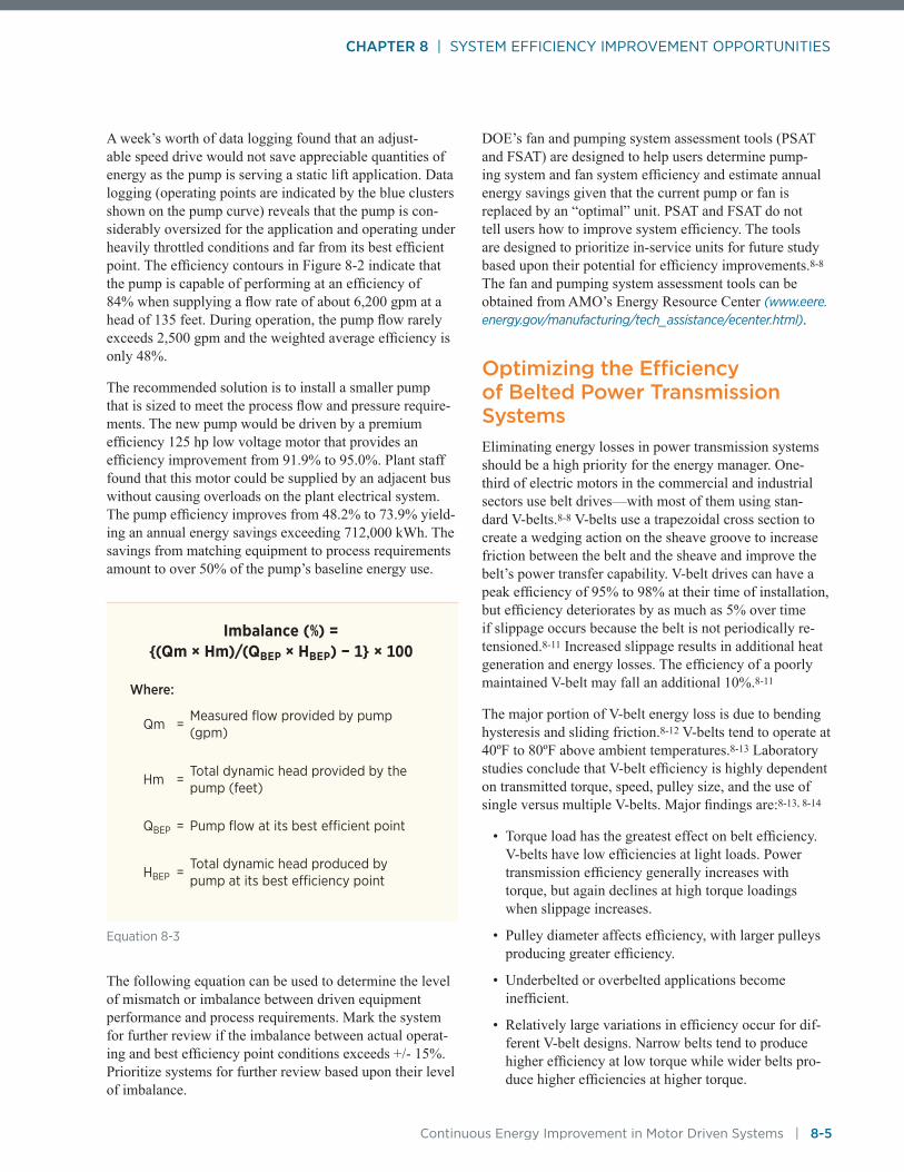
CHAPTER 8 | SYSTEM EFFICIENCY IMPROVEMENT OPPORTUNITIES
Continuous Energy Improvement in Motor Driven Systems | 8-5
A week’s worth of data logging found that an adjust-able speed drive would not save appreciable quantities of energy as the pump is serving a static lift application. Data logging (operating points are indicated by the blue clusters shown on the pump curve) reveals that the pump is con-siderably oversized for the application and operating under heavily throttled conditions and far from its best efficient point. The efficiency contours in Figure 8-2 indicate that the pump is capable of performing at an efficiency of 84% when supplying a flow rate of about 6,200 gpm at a head of 135 feet. During operation, the pump flow rarely exceeds 2,500 gpm and the weighted average efficiency is only 48%.
The recommended solution is to install a smaller pump that is sized to meet the process flow and pressure require-ments. The new pump would be driven by a premium efficiency 125 hp low voltage motor that provides an efficiency improvement from 91.9% to 95.0%. Plant staff found that this motor could be supplied by an adjacent bus without causing overloads on the plant electrical system. The pump efficiency improves from 48.2% to 73.9% yield-ing an annual energy savings exceeding 712,000 kWh. The savings from matching equipment to process requirements amount to over 50% of the pump’s baseline energy use.
The following equation can be used to determine the level of mismatch or imbalance between driven equipment performance and process requirements. Mark the system for further review if the imbalance between actual operat-ing and best efficiency point conditions exceeds +/- 15%. Prioritize systems for further review based upon their level of imbalance.
DOE’s fan and pumping system assessment tools (PSAT and FSAT) are designed to help users determine pump-ing system and fan system efficiency and estimate annual energy savings given that the current pump or fan is replaced by an “optimal” unit. PSAT and FSAT do not tell users how to improve system efficiency. The tools are designed to prioritize in-service units for future study based upon their potential for efficiency improvements.8-8 The fan and pumping system assessment tools can be obtained from AMO’s Energy Resource Center (www.eere.energy.gov/manufacturing/tech_assistance/ecenter.html).
Optimizing the Efficiency of Belted Power Transmission SystemsEliminating energy losses in power transmission systems should be a high priority for the energy manager. One-third of electric motors in the commercial and industrial sectors use belt drives—with most of them using stan-dard V-belts.8-8 V-belts use a trapezoidal cross section to create a wedging action on the sheave groove to increase friction between the belt and the sheave and improve the belt’s power transfer capability. V-belt drives can have a peak efficiency of 95% to 98% at their time of installation, but efficiency deteriorates by as much as 5% over time if slippage occurs because the belt is not periodically re-tensioned.8-11 Increased slippage results in additional heat generation and energy losses. The efficiency of a poorly maintained V-belt may fall an additional 10%.8-11
The major portion of V-belt energy loss is due to bending hysteresis and sliding friction.8-12 V-belts tend to operate at 40ºF to 80ºF above ambient temperatures.8-13 Laboratory studies conclude that V-belt efficiency is highly dependent on transmitted torque, speed, pulley size, and the use of single versus multiple V-belts. Major findings are:8-13, 8-14
• Torque load has the greatest effect on belt efficiency. V-belts have low efficiencies at light loads. Power transmission efficiency generally increases with torque, but again declines at high torque loadings when slippage increases.
• Pulley diameter affects efficiency, with larger pulleys producing greater efficiency.
• Underbelted or overbelted applications become inefficient.
• Relatively large variations in efficiency occur for dif-ferent V-belt designs. Narrow belts tend to produce higher efficiency at low torque while wider belts pro-duce higher efficiencies at higher torque.
Imbalance (%) = {(Qm × Hm)/(QBEP × HBEP) − 1} × 100
Where:
Qm =Measured flow provided by pump (gpm)
Hm =Total dynamic head provided by the pump (feet)
QBEP = Pump flow at its best efficient point
HBEP =Total dynamic head produced by pump at its best efficiency point
Equation 8-3

CHAPTER 8 | SYSTEM EFFICIENCY IMPROVEMENT OPPORTUNITIES
8-6 | Continuous Energy Improvement in Motor Driven Systems
The most important parameter to control in a V-belt drive is the tension. V-belts tend to stretch during their life, causing tension to drop. If belts are too loose, they tend to vibrate, wear rapidly, and waste energy though slippage. If they are too tight, they will also show excessive wear and can dramatically shorten bearing and shaft life. The proper tension of a V-belt is the lowest tension at which the belt will not slip at peak-load conditions.8-10 A properly installed and tensioned V-belt will last from 3 to 5 years. In harsh conditions, service life can decline to a year or less. Belt replacement more than twice a year may be an indication of a serious problem.8-15, 8-16
Notched BeltsTo improve energy efficiency and reduce slippage losses, consider replacing V-belts with notched belts. The simple payback is improved if this action is taken at the time of a belt failure as only the incremental cost of the belt efficiency improvement measure must be considered. A notched V-belt is a direct replacement for a conventional V-belt and can use the same pulleys as an equivalent rated standard V-belt. Notched belts typically have an efficiency 2% higher than the nominal 93% efficiency of standard V-belts.8-17 Notched belts have slots that run perpendicular to the belt’s length (see Figure 8-2). The slots reduce the bending resistance of the belt. They tend to run cooler and last longer than V-belts. While their initial cost is slightly higher, their longer life means that the total cost of pur-chasing new and replacement belts is comparable to that for standard V-belts.
Synchronous BeltsSynchronous belts are toothed and require the installation of mating toothed-drive sprockets. They operate with an efficiency of 98% and maintain that efficiency over a wide torque range.8-17 The recommended tension for a synchro-nous belt is typically less than that for a standard V-belt. This means that motor and driven equipment shaft bear-ings will operate under lower loads, providing a longer service life.8-13 Synchronous belt drives have minimal heat buildup due to low bending stresses and are not prone to efficiency reductions due to slippage. Synchronous belts thus require less maintenance and re-tensioning, can oper-ate in wet and oily environments, and are not affected by abrasive particles. However, they can be noisy, are unsuit-able for shock loads, and transfer vibrations.
Rotating Equipment Speed ConsiderationsCentrifugal fans and pumps exhibit a strong relationship between operating speed and input power requirements. For these applications, synchronous belt sprockets must be selected that take into account the absence of belt slippage. Operating costs would increase if slippage was reduced and the centrifugal load was driven at a slightly higher operating speed. A properly designed synchronous belt drive should ensure that the final rotating equipment speed is equal to the original rotating equipment speed.
For additional information, see DOE’s Motor Systems Energy Tip Sheet #5, Replace V-Belts with Notched or Synchronous Belt Drives (www.eere.energy.gov/ manufacturing/tech_assistance/pdfs/replace_vbelts_motor_systemts5.pdf).
Figure 8-3. Notched and Synchronous Belts. A notched belt, left, runs cooler and has a higher efficiency than a standard V-belt. A synchronous belt, right, can maintain higher efficiency over a wide load range and requires minimal maintenance. Photos from Gates Rubber Company
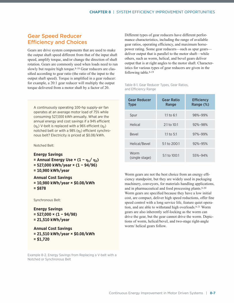
CHAPTER 8 | SYSTEM EFFICIENCY IMPROVEMENT OPPORTUNITIES
Continuous Energy Improvement in Motor Driven Systems | 8-7
Gear Speed Reducer Efficiency and ChoicesGears are drive system components that are used to make the output shaft speed different from that of the input shaft speed, amplify torque, and/or change the direction of shaft rotation. Gears are commonly used when loads need to run slowly but require high torque.8-18 Gear reducers are clas-sified according to gear ratio (the ratio of the input to the output shaft speed). Torque is amplified in a gear reducer: for example, a 20:1 gear reducer will multiply the output torque delivered from a motor shaft by a factor of 20.
Different types of gear reducers have different perfor-mance characteristics, including the range of available gear ratios, operating efficiency, and maximum horse-power rating. Some gear reducers—such as spur gears—deliver output that is parallel to the motor shaft—while others, such as worm, helical, and bevel gears deliver output that is at right angles to the motor shaft. Character-istics for various types of gear reducers are given in the following table.8-19
Worm gears are not the best choice from an energy effi-ciency standpoint, but they are widely used in packaging machinery, conveyors, for materials handling applications, and in pharmaceutical and food processing plants.8-20
Worm gears are specified because they have a low initial cost, are compact, deliver high speed reductions, offer fine speed control with a long service life, feature quiet opera-tion, and are able to withstand high overloads.8-21 Worm gears are also inherently self-locking as the worm can drive the gear, but the gear cannot drive the worm. Depic-tions of worm, helical/bevel, and two-stage right-angle worm/ helical gears follow.
A continuously operating 100-hp supply-air fan operates at an average motor load of 75% while consuming 527,000 kWh annually. What are the annual energy and cost savings if a 94% efficient (η1) V-belt is replaced with a 96% efficient (η2) notched belt or with a 98% (η3) efficient synchro-nous belt? Electricity is priced at $0.08/kWh.
Notched Belt:
Energy Savings = Annual Energy Use × (1 − η1/ η2) = 527,000 kWh/year × (1 − 94/96) = 10,980 kWh/year
Annual Cost Savings = 10,980 kWh/year × $0.08/kWh = $878
Synchronous Belt:
Energy Savings = 527,000 × (1 − 94/98) = 21,510 kWh/year
Annual Cost Savings = 21,510 kWh/year × $0.08/kWh = $1,720
Example 8-2. Energy Savings from Replacing a V-belt with a Notched or Synchronous Belt
Table 8-1. Gear Reducer Types, Gear Ratios, and Efficiency Range
Gear Reducer Type
Gear Ratio Range
Efficiency Range (%)
Spur 1:1 to 6:1 98%–99%
Helical 2:1 to 10:1 92%–98%
Bevel 1:1 to 5:1 97%–99%
Helical/Bevel 5:1 to 200:1 92%–95%
Worm (single stage)
5:1 to 100:1 55%–94%
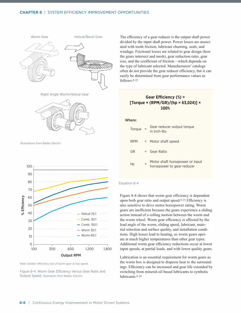
CHAPTER 8 | SYSTEM EFFICIENCY IMPROVEMENT OPPORTUNITIES
8-8 | Continuous Energy Improvement in Motor Driven Systems
The efficiency of a gear reducer is the output shaft power divided by the input shaft power. Power losses are associ-ated with tooth friction, lubricant churning, seals, and windage. Frictional losses are related to gear design (how the gears intersect and mesh), gear reduction ratio, gear size, and the coefficient of friction—which depends on the type of lubricant selected. Manufacturers’ catalogs often do not provide the gear reducer efficiency, but it can easily be determined from gear performance values as follows:8-22
Figure 8-4 shows that worm gear efficiency is dependent upon both gear ratio and output speed.8-23 Efficiency is also sensitive to drive motor horsepower rating. Worm gears are inefficient because the gears experience a sliding action instead of a rolling motion between the worm and the worm wheel. Worm gear efficiency is affected by the lead angle of the worm, sliding speed, lubricant, mate-rial selection and surface quality, and installation condi-tions. High losses lead to heating, so worm gears oper-ate at much higher temperatures than other gear types. Additional worm gear efficiency reductions occur at lower input speeds, at partial loads, and with lower quality gears.
Lubrication is an essential requirement for worm gears as the worm box is designed to disperse heat to the surround-ings. Efficiency can be increased and gear life extended by switching from mineral-oil based lubricants to synthetic lubricants.8-24
Output RPM
% E
�ci
ency
300 600 1,8001,200
Helical 25:1
Comb. 30:1
Comb. 150:1
Worm 30:1
Worm 60:1
100
40
30
20
10
0
50
60
70
80
90
100
Note: Greater efficiency loss of worm gear at low speed
Figure 8-4. Worm Gear Efficiency Versus Gear Ratio and Output Speed. Illustration from Baldor Electric
Gear Efficiency (%) = [Torque × (RPM/GR)/(hp × 63,024)] ×
100%
Where:
Torque =Gear reducer output torque in inch-lbs
RPM = Motor shaft speed
GR = Gear Ratio
hp =Motor shaft horsepower or input horsepower to gear reducer
Equation 8-4
Illustrations from Baldor Electric
Worm Gear Helical/Bevel Gear
Right Angle Worm/Helical Gear

CHAPTER 8 | SYSTEM EFFICIENCY IMPROVEMENT OPPORTUNITIES
Continuous Energy Improvement in Motor Driven Systems | 8-9
Specify high efficiency gear reducers for all new projects or upgrades of existing processes. Retrofit projects are not easy to accomplish as a trained eye and product famil-iarity are needed to identify worm gear drives in a plant setting (helical/bevel gears have a longer box). Focus on applications with high gear ratios. Each gearbox has its own nameplate and sometimes the manufacturer must be provided with a serial number to identify the gear type and operating characteristics. Sometimes just the gearbox can be replaced while other times an integral right angle gear drive motor must be purchased. For a worm gear, the “distance” is measured from the centerline of the worm to the centerline of the worm wheel. Physical constraints—including mounts, couplings, shaft size, and gear reducer centerline to centerline distances—can present retrofit obstacles.
Use Adjustable Speed Drives for Applications with Variable Flow Requirements Historically, applications requiring precise speed con-trol were satisfied by direct current motors, eddy current drives, and hydraulic couplings. Processes that required variable flow control often used a fixed speed motor with flows that regulated the opening or closing of discharge or inlet dampers or throttling valves. Fixed speed changes were obtained by changing out pulley diameters, changing gear ratios, or adjusting variable pitch fan blades.8-26 In the 1980s and 1990s, adjustable or variable speed drives appeared on the market and offered an alternative method of flow control.8-26 Adjustable speed drives (ASDs) are now a mature and widely used energy savings technology.
The speed at which an induction motor rotates is a direct function of the number of poles for which it is wound and the electrical supply frequency. At a constant supply frequency, an induction motor is a fixed speed device.8-27 Because the number of poles on a standard induction motor cannot be changed after it is put into service, the only way to change its speed is to change the frequency of the supplied power.8-27 At a frequency of 60 Hz, a four-pole motor has a synchronous speed of 1,800 RPM. If power is supplied at a frequency of 30 Hz, the motor synchronous speed is reduced to 900 RPM (see Equation 8-5). Providing a variable electrical frequency to a motor turns it from a fixed into a variable speed device. This is the principle used by the predominant form of speed control today, the pulse-width modulated (PWM) variable frequency drive.
Quick Fact
While the energy savings per unit are not huge, the number of gears in operation at a site can be sub-stantial. For example, a large airport might utilize more than 20,000 gear reducers for conveyors and escalators, with 5,000 of these being worm gears.8-23
Consider the energy savings that are possible from changing out a worm gear with an end use or load requirement of 5 hp and a 50:1 gear ratio with a helical/bevel gear. The efficiency of the worm gear is 80% while the equivalent helical/bevel gear efficiency is 95%. The worm gear is driven by a 7.5 hp motor with an efficiency of 91%. Energy savings are determined with the following formula:
Energy Savings (kWh) = (5 hp/0.91) × 0.746 kW/hp × hours/year
× (1/0.8 -1/0.95 )
or
Energy Savings (kWh) = Initial Input kW × hours/year
× (1 –ηWG/ηHB )
Where:
ηWG = the efficiency of the worm gear
ηHB =the efficiency of the helical/bevel gear (in %/100)
Assuming 8,000 hours per year of annual operation, the energy savings are 6,472 kWh/year—equivalent to 15.8% of the initial or baseline annual energy use for the worm gear. At an electrical energy rate of $0.08/kWh, annual savings are $517. Additional energy savings can be obtained when an old standard efficiency gear drive motor is replaced with a new premium efficiency motor. Sometimes, increasing the gear reducer efficiency provides an opportunity to downsize the replacement motor.8-25
Example 8-3 Energy Savings from Use of a Helical/Bevel Gear Instead of a Worm Gear

CHAPTER 8 | SYSTEM EFFICIENCY IMPROVEMENT OPPORTUNITIES
8-10 | Continuous Energy Improvement in Motor Driven Systems
The PWM drive consists of a rectifier, a DC link or inter-mediate circuit, and an inverter (see Figure 8-5). The rectifier converts AC line power to DC power. The DC link conditions the power through the use of harmonic and power ripple filters and also provides power storage using capacitors. The DC voltage is then converted back into AC power at the inverter.
The insulated gate bipolar transistors (IGBTs) used in the inverter section of the ASD have high losses when they create wave shapes other than square waves. To minimize switching losses, drive designers approximate sine waves at different frequencies while operating switches full on or full off. A square wave of much higher frequency than the fundamental is created, usually between 2 kHz and 20 kHz. This is called a carrier wave. Each “on” portion of the carrier wave is called a pulse. The duration of a pulse is called the pulse width. Long pulses produce a high average voltage and brief pulses produce a lower aver-age voltage. The rolling average voltage provided by the
drive is designed to approximate a sinusoidal waveform at the desired frequency.8-28, 8-29 The motor current cannot respond instantaneously, so it tracks the rolling average of voltage over several pulses. Adequate torque is maintained over the entire range of motor operating speeds through regulating the output voltage to maintain a constant volt-age to output frequency (V/Hz) ratio.8-29
In addition to controlling motor speed and torque, PWM ASDs can provide soft start capability (which reduces vibrations and wear on motor bearings), reduced starting current, and correct power factor to 95% upstream of the drive location. Incorporating bypass motor starters into the drive design allows the system to revert to normal constant speed operation in the event of a drive fault. Voltage boost—or the provision of higher than normal voltage to the motor at low speeds—is available for high inertia loads. A common ASD control strategy consists of using sensors and a feedback loop to vary motor and driven equipment speed to maintain pressure, flow, liquid level, torque, dimensions, or temperature at a desired setpoint.8-30 Drives are also well suited for machine tool applications as they allow for continuous and precise speed adjustments.8-27
When considering an ASD for a new or retrofit applica-tion, understanding process requirements is more important than understanding the drive itself.8-27 The remainder of this chapter will focus on factors that influ-ence ASD applicability and energy savings, including:
• Types of loads encountered in industrial applications
• Flow control techniques typically used with pumps and fans
• Static head requirements
Input Converter
Output Inverter
DC Link
Control Circuits
Display Process Feedback/
Control Signal
Operator Controls
Line Voltage
To Motor
Figure 8-5. Variable Frequency Drive Components and Simulated Voltage Waveform
Motor RPM = 120 • f / Poles
Where:
Poles = Number of motor magnetic poles
f = Power supply frequency in Hz
Typical fixed motor speeds at 60 Hz are 3,600 RPM (2-pole), 1,800 RPM (4-pole), 1,200 RPM (6-pole), and 900 RPM (8-pole)
Equation 8-5
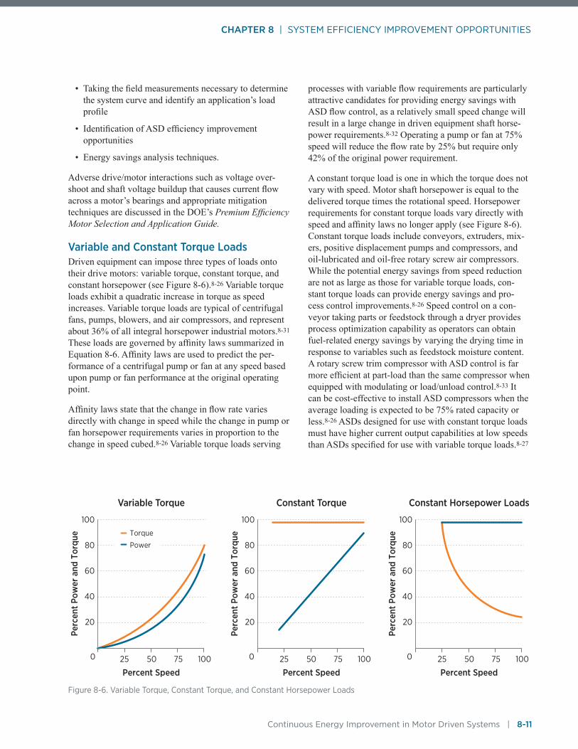
CHAPTER 8 | SYSTEM EFFICIENCY IMPROVEMENT OPPORTUNITIES
Continuous Energy Improvement in Motor Driven Systems | 8-11
• Taking the field measurements necessary to determine the system curve and identify an application’s load profile
• Identification of ASD efficiency improvement opportunities
• Energy savings analysis techniques.
Adverse drive/motor interactions such as voltage over-shoot and shaft voltage buildup that causes current flow across a motor’s bearings and appropriate mitigation techniques are discussed in the DOE’s Premium Efficiency Motor Selection and Application Guide.
Variable and Constant Torque LoadsDriven equipment can impose three types of loads onto their drive motors: variable torque, constant torque, and constant horsepower (see Figure 8-6).8-26 Variable torque loads exhibit a quadratic increase in torque as speed increases. Variable torque loads are typical of centrifugal fans, pumps, blowers, and air compressors, and represent about 36% of all integral horsepower industrial motors.8-31 These loads are governed by affinity laws summarized in Equation 8-6. Affinity laws are used to predict the per-formance of a centrifugal pump or fan at any speed based upon pump or fan performance at the original operating point.
Affinity laws state that the change in flow rate varies directly with change in speed while the change in pump or fan horsepower requirements varies in proportion to the change in speed cubed.8-26 Variable torque loads serving
processes with variable flow requirements are particularly attractive candidates for providing energy savings with ASD flow control, as a relatively small speed change will result in a large change in driven equipment shaft horse-power requirements.8-32 Operating a pump or fan at 75% speed will reduce the flow rate by 25% but require only 42% of the original power requirement.
A constant torque load is one in which the torque does not vary with speed. Motor shaft horsepower is equal to the delivered torque times the rotational speed. Horsepower requirements for constant torque loads vary directly with speed and affinity laws no longer apply (see Figure 8-6). Constant torque loads include conveyors, extruders, mix-ers, positive displacement pumps and compressors, and oil-lubricated and oil-free rotary screw air compressors. While the potential energy savings from speed reduction are not as large as those for variable torque loads, con-stant torque loads can provide energy savings and pro-cess control improvements.8-26 Speed control on a con-veyor taking parts or feedstock through a dryer provides process optimization capability as operators can obtain fuel-related energy savings by varying the drying time in response to variables such as feedstock moisture content. A rotary screw trim compressor with ASD control is far more efficient at part-load than the same compressor when equipped with modulating or load/unload control.8-33 It can be cost-effective to install ASD compressors when the average loading is expected to be 75% rated capacity or less.8-26 ASDs designed for use with constant torque loads must have higher current output capabilities at low speeds than ASDs specified for use with variable torque loads.8-27
Percent Speed
Perc
ent P
ower
and
Tor
que
50 75 100250
20
40
60
80
100
50 75 100250 50 75 100250
Percent Speed
Perc
ent P
ower
and
Tor
que
20
40
60
80
100
Percent Speed
Variable Torque Constant Torque Constant Horsepower Loads
Perc
ent P
ower
and
Tor
que
20
40
60
80
100
Torque
Power
Figure 8-6. Variable Torque, Constant Torque, and Constant Horsepower Loads

CHAPTER 8 | SYSTEM EFFICIENCY IMPROVEMENT OPPORTUNITIES
8-12 | Continuous Energy Improvement in Motor Driven Systems
At constant horsepower load, the delivered torque var-ies inversely with speed. Examples of this type of load include lathes, drilling, or milling machines where heavy cuts are made at low speed and light cuts are made at high speed. These applications do not provide energy savings when the driven equipment speed is reduced.8-29
Fan and Pump Performance Curves, System Curves, and Flow Regulation with Throttling Valves and Inlet or Outlet DampersCentrifugal pumps and fans can serve a wide range of operating conditions. A fan or pump characteristics or performance curve is a plot of possible pressure (head) and delivered flow operating points. Those conducting
energy studies should always ask the maintenance staff for copies of pump and fan curves. If they are not available at the plant, contact the manufacturer and provide nameplate information, including the serial number. A pump curve is referenced to an operating speed and usually indicates impeller diameter, gpm, head in feet, efficiencies at different operating points, and suction head and brake horsepower requirements. A fan performance curve graphically depicts cfm, static or total pressure (in-wg), revolutions per minute, and brake horsepower requirements.8-34 A fan curve might reflect the movement of air or industrial gases at a stated process temperature. Performance curves are independent of the system into which the pump or fan is installed.
A system curve is a representation of the relationship between flow and losses in a given piping or ducting system. Losses are a function of rate of flow, size (diameter or cross-sectional area), surface roughness, length of pipe or duct, and number, size, and type of valves, elbows, and fittings. Additional entrance and exit hydraulic losses occur as well as losses due to changes in pipe size by sudden or gradual enlargements or reductions in pipe diameter.8-35 System curves are developed by those involved in process design or can be obtained by taking field measurements of pump or fan pressure and flow. A system curve shows how much pressure is required from the pump or fan to overcome system losses and produce a given fluid flow.8-32 The system curve is independent of the pump or fan selection. The intersection of the pump or fan performance and system curves defines the actual pump or fan operating point.8-35 This operating point is associated with a specific set of pressure, flow, efficiency, and shaft horsepower values.
Pumps and fans are often oversized. Accurately calculat-ing friction losses or pressure drops in the piping or duct-ing system is a difficult task and safety margins are usually added during the design phase.8-36 Due to this oversiz-ing, pumps and fans are rarely called upon to operate at their rated capacity. In addition, pumps and fans are often installed in systems with multiple operating points that coincide with varying process requirements. This oversiz-ing works against the cardinal rule of fan system effi-ciency: to move only the amount of air necessary because power consumption often varies with the cube of the air flow volume.8-37
Flow control for fans is often provided by discharge or outlet dampers, inlet guide vanes, or a combination of the two. Outlet dampers control the gas after it has passed through the fan by changing the resistance that the fan is working against.8-38 With radial-blade and forward
Affinity Laws that govern centrifugal fan and pump operation are:
Q2 / Q1 = RPM2 / RPM1, H2 / H1 = (RPM2 / RPM1)2
P2 / P1 = (H2 × Q2) / (H1 × Q1) = (RPM2 / RPM1)3
Where:
Q =
Fluid flow in gallons per minute (gpm), gas volume flow in cubic feet per minute (cfm)
RPM =Pump or fan rotational speed, revolutions per minute
H =Head in feet or pressure in inches-wc (inches of water column)
P = Brake or shaft horsepower
Q1, H1, P1, RPM1 =Pump or fan performance at normal (initial) operating point
Q2, H2, P2, RPM2 = Pump or fan performance at final operating point
Equation 8-6. The Affinity Laws

CHAPTER 8 | SYSTEM EFFICIENCY IMPROVEMENT OPPORTUNITIES
Continuous Energy Improvement in Motor Driven Systems | 8-13
Percent Flow
20 40 60 80 100 120 140 1600
Percent Flow
20 40 60 80 100 120 140 1600
140 140
Perc
ent P
ress
ure
20
40
60
80
100
120
Perc
ent I
nput
Pow
er
20
40
60
80
100
120
Fan Performance Curve
60% speed
100% speed
80% speed
Percent Flow
Perc
ent P
ress
ure
20 40 60 80 100 120 140 160
20
40
60
80
100
120
Percent Flow
Perc
ent I
nput
Pow
er
20 40 60 80 100 120 140 1600 0
20
40
60
80
100
120
140 140
Full open
Fan Performance Curve
¼ open
½ open
Percent Flow
Perc
ent P
ress
ure
20 40 60 80 100 120 140 160
20
40
60
80
100
120
140
Percent Flow
Perc
ent I
nput
Pow
er
20 40 60 80 100 120 140 160
20
40
60
80
100
120
140
0 0
Fan Performance Curve
System Curves
Figure 8-7. Discharge Damper Flow Regulation
Figure 8-8. Inlet Damper or Inlet Guide Vane Flow Control
Figure 8-9. Adjustable Speed Flow Control
CHAPTER 8 | SYSTEM EFFICIENCY IMPROVEMENT OPPORTUNITIES
8-14 | Continuous Energy Improvement in Motor Driven Systems
curved-fans, the dampered horsepower will be less than the unregulated horsepower as the fan moves to the left on its performance and brake horsepower (BHP) curves. With backwardly inclined fans, the dampered horsepower may be less, the same, or more than the wide open horsepower, depending upon the original operating point.8-38
Axial fans offer flow modulation when they are equipped with adjustable or variable pitch (adjustable “in flight”) fan blades. Unlike fixed blade fans, adjustable pitch fans allow users to change the blade angle settings and “tune” the flow provided to meet process requirements.8-39 Some large adjustable pitch fans cannot be re-set “on the fly.” They must be shut down to allow the blade angle to be adjusted, and then restarted with the appropriate starter so the correct breakers and circuit protection are functioning. Adjustable and variable pitch blades allow for efficient flow volume control without changing the speed of the fan.8-39
For pumps, a throttling valve is usually employed when the process flow requirement is less than the flow provided at a pumping system’s natural operating point. Similar to discharge dampers on a fan, pump throttling valves mod-ify the system curve and provide flow control by increas-ing the system’s resistance to flow. This increase in pres-sure or head requirements results in a change in the system curve due to the pressure drop and energy loss across the discharge damper or throttling valve. The operating point (defined by the intersection of the system and fan or pump performance curve) shifts to the left along the fan or pump performance curve. Fan horsepower requirements gradu-ally decrease when discharge dampers are used to reduce flow (see Figure 8-7).8-32 Pumps and fans that operate to the left of their best efficiency point (BEP) suffer addi-tional losses in efficiency as operation shifts to a lower efficiency point.
Fan inlet dampers or inlet guide vanes are widely used as they are more efficient than outlet damper flow regula-tion. These dampers are a common volume control device because they are low in cost, require little maintenance, easily adjust airflow during operation, and require little space.8-38 Inlet dampers pre-spin the incoming air in the same direction as the fan wheel rotation.8-38, 8-40 This directed air movement reduces fan output pressure and airflow, thus reducing the shaft horsepower require-ments that the fan imposes on its drive motor. As shown in Figure 8-8, the inlet dampers create a new fan perfor-mance curve for every damper position, intersecting the system curve at different points.8-32, 8-40 Inlet damper flow regulation is more efficient than using outlet dampers as the horsepower requirements at reduced flows drop to a greater extent.8-32
ASDs are almost always more efficient than throttling valves or outlet dampers as they make it possible to adjust the flow to the demand without throttling and its associ-ated losses.8-36 With adjustable speed flow control, fan and pump performance curves follow the Affinity Laws and the operating point occurs at the intersection of the system curve and the reduced speed driven-equipment curve. For variable torque systems with no static lift or fixed pres-sure drop requirements, the input power requirements vary as the cube of the speed ratio. As shown in the “% Input Power versus % Flow” portion of Figure 8-9, ASD flow control can produce significant energy savings at reduced flows when compared to discharge damper or inlet guide van flow control.8-31 ASD flow control is appropriate for retrofit applications or new system designs. For new systems, the capital costs of the ASD may be offset by reductions in control valve costs and conventional motor starters.8-41
Dampers are restricted in their ability to severely restrict airflow. When airflow is reduced by as much as 70%, flow instability or rotating stall may occur.8-40 These condi-tions can result in vibration and fan casing cracking. For existing fan or pumping systems equipped with mechani-cal throttling valve or damper flow control, ASD flow regulation is more efficient and should be considered as a potential energy savings retrofit opportunity. After installing an ASD, a damper or throttling valve can be left fully open (or removed) with flows regulated entirely through speed control. ASD flow control can also save a considerable amount of energy in pumping systems with recirculation or bypass flow control. With this technique, the pump operates at a constant output with unneces-sary discharge returned to the pump inlet or the tank from which the pump takes suction. Overall, centrifugal fan and pump applications are ideal for ASD flow regulation as they usually do not have high startup or breakaway torque requirements, there is rarely a need for high acceleration or deceleration, they are not exposed to shock loading or overloading conditions, and they do not require braking capability.8-42
Applications with Static Head Requirements In a pumping system, the system curve indicates the pumping head that is required to produce a given flow rate. A system curve is comprised of both static head and dynamic or friction loss components. In the absence of static head, the system-head curve starts at zero flow and zero head.8-35 Static head is the pressure required to over-come an elevation change or fixed pressure drop in the system. Static head requirements are independent of flow while friction head losses are generally proportional to the square of the flow rate. The system curve is represented by

CHAPTER 8 | SYSTEM EFFICIENCY IMPROVEMENT OPPORTUNITIES
Continuous Energy Improvement in Motor Driven Systems | 8-15
a horizontal line in a pumping system with only static lift requirements. When both static lift and friction losses are present, the system curve starts at the static head and zero flow point on the head-capacity curve.8-35 Friction losses at each flow point are added to the static life requirements to determine the system curve.
For static head dominated pumping systems, a substantial amount of the input energy is required for lifting fluid or overcoming fixed pressure requirements. An ASD can-not reduce the pumping power required to increase the potential energy of a quantity of fluid when it is raised to a higher elevation. ASD-related power reductions occur
from pumping less fluid per unit of time and thereby decreasing the dynamic or friction losses in the pipes.8-43
Affinity laws do not apply and should not be used to esti-mate energy savings in systems with significant static head requirements. In static lift dominated systems, a small change in pump or fan speed can result in a large variation in fluid flow. Special care must be taken when analyzing systems with a large amount of static head. When speed is reduced with an ASD, the operating point of a pumping system rapidly shifts to the left until no fluid flow occurs and a pump is “dead-headed.” Severe damage can occur if a pump is operated under these conditions for an
Static head
System curve
Pump e�ciency contours100% 90% 80% 70%Speed:
Hea
d in
Fee
t
Flow Rate in Gallons Per Minute
200
150
100
50
1,0000
30% 40%
75%
75%
80.5%(BEP)
2,000 4,0003,000 5,000
70%80%
90%100%
50% 60%70%
Hea
d in
Fee
t
200
150
100
50
30% 40%
75%
80.5%(BEP)
Pump e�ciency contours
System curve
70%80%
90%
100%
100% 90% 80% 70%Speed:
Flow Rate in Gallons Per Minute
1,0000 2,000 4,0003,000 5,000
50% 60% 70%75%
Figure 8-10. System Curve From Friction Losses Only
Figure 8-11. System Curve with a Static Head Requirement

CHAPTER 8 | SYSTEM EFFICIENCY IMPROVEMENT OPPORTUNITIES
8-16 | Continuous Energy Improvement in Motor Driven Systems
extended period of time.8-36 Precise knowledge of the pump curve, pump efficiency at each operating point, and the system curve is required to determine the pump horse-power required at each discharge rate in a static head-dominated system.
Static head applications are common in industrial fan and pumping applications. Pumping examples include submersible well pumps that discharge into a reservoir or directly into a pressurized water distribution pipeline, process or booster pumps that supply water to an elevated or pressurized tank, feedwater pumps that inject returned condensate and makeup water into a fire tube or water tube steam boiler, and pumps that must overcome a fixed pres-sure drop in a sprinkler or spray nozzle for droplet atomi-zation. Blowers at wastewater treatment plants with full bottom coverage aeration systems must overcome the pres-sure due to the water column above the bubble emitter plus the pressure drop across the diffuser. Induced draft fans often must supply a constant negative pressure at the flue of a boiler or other pickup; provide gas flows that yield a fixed pressure drop across a Venturi scrubber; or overcome the pressure drop across the filter fabric in a baghouse.
Figure 8-10 shows a system curve for a system that is totally dominated by friction losses, such as a circulating hot water loop in a heating system.8-41 The operating point (3,500 gpm, 90 feet of head) is just to the right of the BEP for this system. As the pump speed is reduced, deliv-ered flow and pressure decreases but the pump efficiency remains above 80%. This is because efficiency isopleths (lines of constant pump efficiency, shown in white in Fig-ure 8-10) and the system curve (shown in dark blue) both move toward the zero-flow/zero-head origin on the head/capacity graph (see Figure 8-10).8-41
A system dominated by static head requirements behaves in a different manner. Small changes in pump or fan speed result in large changes in flow. The system curve shown in Figure 8-11 has a static requirement of 65 feet and inter-sects the pump curve at the same operating point as Figure 8-10.8-41 In the friction dominated system, the flow rate would be about 2,400 gpm at 70% speed with the pump efficiency maintained at around 80%. When the speed of the pump is reduced to 70% of its original operating speed in the static head application, the flow rate is reduced to about 800 gpm and the pump efficiency decreases to about 55%.
In a system with only static head, the pump efficiency loss effect is even more dramatic and energy use could increase if an ASD was used for flow regulation. In the example shown, the pump would “dead-head” and provide no flow
whatsoever if operated at 70% speed. The pump is not capable of producing enough pressure to overcome static lift requirements and move water. Energy savings poten-tial decreases as static head—expressed as a percentage of total system head requirements—increases.8-27 On-off con-trol of pumps is a very efficient flow control strategy for high static lift applications, such as a well pump delivering water to an elevated reservoir.
Duty Cycle and Load ProfilesThe duty cycle for a system indicates how many hours per year it is in operation. The load profile shows how process flow requirements fluctuate when the system is in opera-tion. Valuable information is often available from operat-ing records, discussions with operating staff, plant supervi-sory control systems, or continuous emissions monitoring equipment. For instance, boiler steam production and exhaust gas flow and temperatures at the plant stack might be available at 14-minute intervals over the preceding operating year. Given variable boiler steam production, a week’s worth of power logging might allow the energy manager to determine baseline the annual energy use and the load profile for the boiler’s forced or induced draft fan.
Field measurements often must be made to determine the load profile. Liquid flow measurements can be logged with a non-intrusive transit-time flowmeter. A recording annubar can be used to determine gas flows over time. An RMS power meter should be used to determine input power to the driven-equipment drive motor over the same time the flow measurements are taken. Recording data for at least a week is recommended.
Once flow measurements are made, separate the avail-able data into flow “bins.” Each bin might represent a range of flow values, for instance greater than or equal (>=)30% and < 35% of full-flow. Count the number of measured flow values in each bin and divide by the total count to determine the fraction of operating time associ-ated with each bin. A histogram graphically depicts an application’s flow profile or variable flow requirements by indicating the percentage of operating time that flows fall within each specified flow range. ASD energy sav-ings increase when duty cycles are high and the system operates far from its full-flow operating point. Figure 8-12 illustrates a load profile that indicates an “excellent” ASD retrofit opportunity. Figure 8-13 shows an application that is not as attractive as the one shown in Figure 8-12, but still offers “good” ASD energy savings potential. A “poor” ASD retrofit candidate is indicated by the load profile in Figure 8-14.8-27 Remember that an ASD will actually increase energy consumption at full-flow due to losses in the drive’s power electronics.
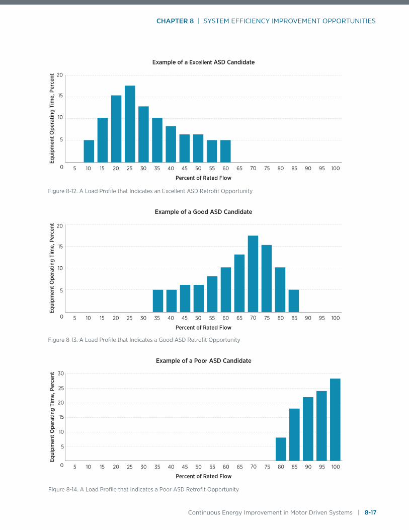
CHAPTER 8 | SYSTEM EFFICIENCY IMPROVEMENT OPPORTUNITIES
Continuous Energy Improvement in Motor Driven Systems | 8-17
0
30
25
20
15
10
5
Equi
pmen
t Ope
ratin
g Ti
me,
Per
cent
Percent of Rated Flow
10 20 30 40 45 503515 255 55 65 75 85 95 1009070 8060
Example of a Poor ASD Candidate
20
15
10
5
Equi
pmen
t Ope
ratin
g Ti
me,
Per
cent
Percent of Rated Flow
0 10 20 30 40 45 503515 255 55 65 75 85 95 1009070 8060
Example of a Excellent ASD Candidate
Equi
pmen
t Ope
ratin
g Ti
me,
Per
cent
Percent of Rated Flow
10 20 30 40 45 503515 255 55 65 75 85 95 1009070 8060
Example of a Good ASD Candidate
20
15
10
5
0
Figure 8-12. A Load Profile that Indicates an Excellent ASD Retrofit Opportunity
Figure 8-13. A Load Profile that Indicates a Good ASD Retrofit Opportunity
Figure 8-14. A Load Profile that Indicates a Poor ASD Retrofit Opportunity

CHAPTER 8 | SYSTEM EFFICIENCY IMPROVEMENT OPPORTUNITIES
8-18 | Continuous Energy Improvement in Motor Driven Systems
A duty cycle that indicates throttling or damper control is employed to provide a constant flow that is less than full-flow indicates that other efficiency measures should be considered. These might include changing out pulley sizes for belted loads, trimming a pump impeller, replacing the equipment drive motor with one with a lower synchro-nous speed (such as replacing an 1,800 RPM motor with a 1,200 RPM motor), or replacement of an oversized fan or pump with one that is matched to load requirements.
Electronic ASDs should be considered as potential replacements for adjustable belt pulley drives, hydraulic or fluid drives, and eddy current clutches.8-44 See DOE Motor Systems Tip Sheet #12, Is it Cost-Effective to Replace Old Eddy-Current Drives? (www.eere.energy.gov/manufactur-ing/tech_assistance/pdfs/motor_tip_sheet12.pdf) for more information on this potential energy savings opportunity.
In addition to duty cycle and load profile, ASD cost-effec-tiveness is strongly affected by utility rates and possible utility incentives for the investment in efficient equipment. ASDs might be desirable to plant management for reasons other than energy savings. When examining an ASD retro-fit project, secondary benefits should be quantified to the degree possible. Advantages of ASDs can include:8-30
• Improved process control
• Better controllability/controls speed variations or swings
• Fast response
• High acceleration and deceleration
• Increased productivity
• Improved product quality/reduction in reject rates
• Increased equipment life
• Eliminates startup impacts causing system vibrations
• Reduced maintenance costs
• Regeneration
• Supports low current soft starts
• Provides fault tolerance
• Power factor improvement
• Can restart spinning loads
• Less downtime.
Part-Load Efficiency of Motors and Adjustable Speed DrivesThe input power to a pump is proportional to the hydraulic horsepower produced divided by the product of the pump efficiency, motor efficiency, and drive efficiency at their respective operating and load points.
When a pump is throttled, its operating point is at the inter-section of the pump performance curve and the desired flow rate. When ASD flow control is used, the operating point is at the intersection of the systems curve and the desired flow rate. The hydraulic horsepower is propor-tional to the product of the delivered head times the flow at the operating point. The pump shown in Figure 8-15 provides about 900 gpm at a head of 41 feet when running
Figure 8-15. Pump with Unregulated Flow, Throttled Flow Control, and ASD Flow Regulation
Flow in Gallons Per Minute
400 600 800 1000200
Hea
d in
Fee
t
10
20
30
40
50
60
0
Flow in Gallons Per Minute
400 600 800 1000200
Hea
d in
Fee
t
Hea
d in
Fee
t
10
20
30
40
50
60
0
Flow in Gallons Per Minute
400 600 800 1000200
10
20
30
40
50
60
0
Pump CurveSystem Curve

CHAPTER 8 | SYSTEM EFFICIENCY IMPROVEMENT OPPORTUNITIES
Continuous Energy Improvement in Motor Driven Systems | 8-19
P = (Q × H × SG) / (K × ηPUMP × ηASD × ηMOTOR)
Where:
P = Input power in kW
Q = Fluid flow in gallons per minute
H = Head developed by the pump in feet
K =Constant equal to 5,308 for the units given
SG =Specific gravity of the fluid being pumped
ηPUMP = Efficiency of the pump at its operating point
ηASD =Efficiency of the ASD at its operating speed and torque
ηMOTOR =Efficiency of the motor at its load point
Equation 8-7
P = (CFM × SP) / (K × ηFAN × ηASD × ηMOTOR)
Where:
P = Input power in kW
CFM = Volume flow rate (ft3/min)
SP = Static pressure produced by the fan (in-wg)
K =Constant equal to 8,520 for the units given
ηFAN =Efficiency of the fan at its operating point
ηASD =Efficiency of the ASD at its operating speed and torque
ηMOTOR =Efficiency of the motor at its load point
Equation 8-8
at its natural operating point. When throttled to provide a flow of 600 gpm, the head increases to about 46 feet. Use of an ASD for flow control provides the same flow (600 gpm) with a head requirement of only 19 feet. Hydrau-lic horsepower requirements—proportional to the shaded areas shown in Figure 8-15—are significantly reduced.
The input power required by a pump drive motor is: Simi-larly, the input power required by a fan drive motor is:8-45
To determine fan or pump input power requirements at each operating point, the fan or pump, ASD, and motor efficiencies must be determined. Fan and pump efficien-cies can be obtained from performance curves, or, in cases where pump wear and loss of performance is expected; by taking electrical, fluid flow, and pressure measurements and then calculating the rotating equipment efficiency using Equations 8-7 and 8-8.
There is currently no recognized standard for ASD effi-ciency although the Canadian Standards Association (CSA) has proposed a draft standard CSA C838 that uses
the output/input method to determine ASD motor and motor/drive system efficiency. The IEC also released draft standard 60034-2-3 for the determination of motor effi-ciency when fed by a converter waveform.8-46
ASD losses are comprised of two components: conduction losses and switching losses.8-47 Conduction losses do not vary with switching frequency and are equal to the product of the voltage drop across the drive and the current pass-ing through the drive. Switching losses increase in propor-tion to switching frequency.8-47 Both losses result in heat production and elevated drive temperatures.
Test laboratories are beginning to test ASDs to determine their efficiency both with and without being coupled to a drive motor. By testing at four speeds (100%, 75%, 50%, and 25% of rated) and four loads (100%, 75%, 50%, and 25% of full-rated torque) an efficiency contour map can be created.8-48 The efficiency map shown in Figure 8-17 is a new approach to presenting drive and motor performance and illustrates how the combined ASD and drive motor
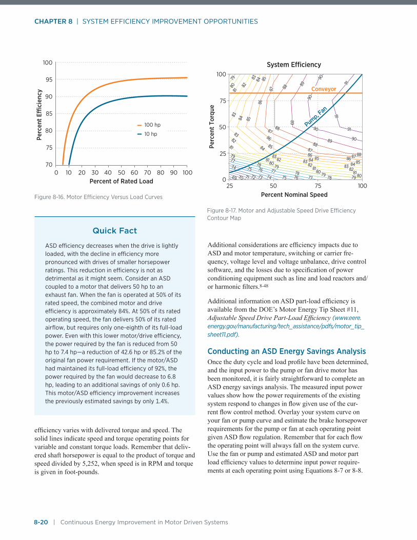
CHAPTER 8 | SYSTEM EFFICIENCY IMPROVEMENT OPPORTUNITIES
8-20 | Continuous Energy Improvement in Motor Driven Systems
efficiency varies with delivered torque and speed. The solid lines indicate speed and torque operating points for variable and constant torque loads. Remember that deliv-ered shaft horsepower is equal to the product of torque and speed divided by 5,252, when speed is in RPM and torque is given in foot-pounds.
Additional considerations are efficiency impacts due to ASD and motor temperature, switching or carrier fre-quency, voltage level and voltage unbalance, drive control software, and the losses due to specification of power conditioning equipment such as line and load reactors and/or harmonic filters.8-48
Additional information on ASD part-load efficiency is available from the DOE’s Motor Energy Tip Sheet #11, Adjustable Speed Drive Part-Load Efficiency (www.eere.energy.gov/manufacturing/tech_assistance/pdfs/motor_tip_sheet11.pdf).
Conducting an ASD Energy Savings AnalysisOnce the duty cycle and load profile have been determined, and the input power to the pump or fan drive motor has been monitored, it is fairly straightforward to complete an ASD energy savings analysis. The measured input power values show how the power requirements of the existing system respond to changes in flow given use of the cur-rent flow control method. Overlay your system curve on your fan or pump curve and estimate the brake horsepower requirements for the pump or fan at each operating point given ASD flow regulation. Remember that for each flow the operating point will always fall on the system curve. Use the fan or pump and estimated ASD and motor part load efficiency values to determine input power require-ments at each operating point using Equations 8-7 or 8-8.
Quick Fact
ASD efficiency decreases when the drive is lightly loaded, with the decline in efficiency more pronounced with drives of smaller horsepower ratings. This reduction in efficiency is not as detrimental as it might seem. Consider an ASD coupled to a motor that delivers 50 hp to an exhaust fan. When the fan is operated at 50% of its rated speed, the combined motor and drive efficiency is approximately 84%. At 50% of its rated operating speed, the fan delivers 50% of its rated airflow, but requires only one-eighth of its full-load power. Even with this lower motor/drive efficiency, the power required by the fan is reduced from 50 hp to 7.4 hp—a reduction of 42.6 hp or 85.2% of the original fan power requirement. If the motor/ASD had maintained its full-load efficiency of 92%, the power required by the fan would decrease to 6.8 hp, leading to an additional savings of only 0.6 hp. This motor/ASD efficiency improvement increases the previously estimated savings by only 1.4%.
Figure 8-16. Motor Efficiency Versus Load Curves
Percent of Rated Load
Perc
ent E
�ci
ency
100 20 30 40 50 60 70 80 90 10070
75
80
85
90
95
100
100 hp
10 hp
Figure 8-17. Motor and Adjustable Speed Drive Efficiency Contour Map
System E�ciency
Percent Nominal Speed
Perc
ent T
orqu
e
100
25
25
50
75
50 75 1000
Conveyor
Pump, Fan
7069 71 72 73
74
74
75
75
76
76
77
77
78
7878
79
797779
79
81
82
83
84
84
85
8384 85
8687
88
88
8986
8788
8182
8385
88
89
84 8586
87
89
90
90
90
90
91
91
91
80
80
8081
8182
82 8383
7980
81
82
83
8485 86 87

CHAPTER 8 | SYSTEM EFFICIENCY IMPROVEMENT OPPORTUNITIES
Continuous Energy Improvement in Motor Driven Systems | 8-21
Table 8-2. Energy Savings Due to Retrofit of an ASD onto a Centrifugal Fan with Discharge Damper Flow Control
% of Rated Flow
% of Operating Time
Annual Operating Hours
Discharge Damper Control, kW
ASD Flow Control, kW
Savings, kWh per year
60 1 80 91 34 4,560
55 2 160 86 30 8,960
50 17 1,360 82 23 80,240
45 12 960 76 15 58,560
40 15 1,314 72 11 80,154
35 13 1,040 70 10 62,400
30 24 1,920 68 9 113,280
25 9 720 65 7 41,760
20 7 560 62 6 31,360
Total Expected Annual Energy Savings, kWh 481,274
Perc
ent o
f Ove
rall
Ope
ratio
nal T
ime
FD F
an M
otor
kW
Combustion Air Fan Flowrate as Percent of Full-Rated Flow
30
25
20
15
10
5
0
100
90
80
70
60
50
40
30
20
10
020 25 30 40 45 50 55 60 70 8035
Percent of Operational Time
Power Curve for Discharge Damper Flow ControlPower Curve for ASD Flow Control
Figure 8-18. Load Profile, Baseline, and ASD Power Requirements Curves for a Combustion Air Supply Fan

CHAPTER 8 | SYSTEM EFFICIENCY IMPROVEMENT OPPORTUNITIES
8-22 | Continuous Energy Improvement in Motor Driven Systems
All of the information necessary for an energy savings analysis is shown on Figure 8-18. The load profile or percent of operating time at each flow point is indicated in blue and is read on the left vertical axis. The orange curve shows how the measured power responds to changes in flow when fan outlet dampers are used. Input kW values are shown on the right vertical axis. The light blue curve shows the estimated input power requirements for the 200 hp drive motor given the use of ASD flow control for the same fan. Expected input kW values are again shown on the right axis. The power savings at each operating or flow
point is the difference between the kW requirements when outlet dampers are deployed less the power required when ASD flow control is provided.
An ASD energy savings analysis can quickly be done on a spreadsheet after using a regression analysis to provide equations that replicate or “fit” the outlet damper and ASD input power responses to changes in flow. A bin analysis is shown in Table 8-2 for the combustion air fan perfor-mance depicted in Figure 8-18 assuming an 8,000-hour duty cycle.
The energy savings analysis shows an expected energy savings of 481,274 kWh per year. This annual energy sav-ings is $38,500 given an energy cost of $0.08/kWh. The total installed cost would be approximately $42,000 for a 200-hp rated ASD in a filtered NEMA 1 enclosure, with automatic bypass control, circuit protection, a 3% line reactor, dV/dt filter, and with a shaft grounding brush for the fan drive motor. The simple payback for this project is about 1.1 years.
Additional information on how to identify and analyze ASD retrofit opportunities is available in the DOE Pump-ing Systems Tips Sheets #11, Adjustable Speed Pumping Applications (www.eere.energy.gov/manufacturing/tech_assistance/pdfs/motor_tip_sheet11.pdf) and #12, Control Strategies for Centrifugal Pumps with Variable Flow Rate Requirements (www.eere.energy.gov/manufacturing/tech_assistance/pdfs/38949.pdf). Also refer to the DOE publica-tion, Improving Motor and Drive System Performance: A Sourcebook for Industry.
Table 8-3. NEMA Designated Enclosures for Electrical Equipment
Designation Protection
NEMA 1Enclosure designed for indoor use protecting components within from physical contact with operating and maintenance personnel.
NEMA 3REnclosure designed for outdoor use. These enclosures protect against falling rain, sleet, and external ice formation.
NEMA 12Enclosure designed for indoor use. Provides protection against dust and dripping liquids, including protection against fibers, lint, dust, dirt, and non-corrosive dripping liquids.
NEMA 4Enclosure designed for indoor and outdoor use. Protects against dirt, dust, splashing water, falling water, seepage, hose-directed water, and external condensation.
NEMA 4X Same as NEMA 4 except the enclosure is corrosion resistant.
Quick Fact
ASDs are sometimes used to slow a large fan or pump drive motor down during short time intervals when process requirements are reduced or do not exist. Large motors cannot be shut down and restarted due to heat production in the motor windings due to high starting currents. Reducing the speed of an 1,800 RPM motor to 400 RPM is almost equivalent to turning it off as, for variable torque loads, the input power requirement of the load drops to only1% of its full-flow value. Examples include washdown or spray systems while a new rail car is being positioned, control of mine ventilation fans during zero staff in mine periods, and control of air pollution control equipment baghouse fans when an electric arc furnace is removed for tapping.

CHAPTER 8 | SYSTEM EFFICIENCY IMPROVEMENT OPPORTUNITIES
Continuous Energy Improvement in Motor Driven Systems | 8-23
ASD Selection Considerations The output rating of an ASD should be based upon the motor nameplate rated full-load current.8-47, 8-49 ASDs should not be selected based upon motor horsepower rat-ing. The motor must be selected and/or protected against ASD-induced voltage overshoots and shaft bearing cur-rents (see “Motor Interactions with Adjustable Speed Drives” and “Guidance for Selecting Motors Controlled by an ASD” sections from DOE’s Premium Efficiency Motor Selection and Application Guide).
Ensure that your ASD comes in an enclosure that is suit-able for your site environmental conditions. Following is a summary of NEMA enclosure designations:8-49
NEMA Standard 250 contains additional information on enclosure classifications. For NEMA 1 enclosures, ventila-tion air may be required for cooling purposes. Depend-ing upon site conditions, filtered air may be required. The ASD enclosure should be equipped with space heaters if the ambient temperature is expected to dip below freezing (0ºC).8-47, 8-49
ASDs can be equipped with a number of control tech-niques. Volts to hertz (V/Hz) control maintains a constant ratio between the drive’s output voltage and frequency to provide a constant full-load torque over the drive’s speed or operating range. Vector control separately controls the magnetizing flux producing and torque producing currents supplied to the motor. The result is accurate speed and torque control that is comparable to that obtained with a DC motor.8-49
Voltage boost is often provided with V/Hz control when the motor is operated at frequencies below 20 Hz. This capability is necessary to provide sufficient locked rotor and breakaway torque without requiring excessive current.8-47
Bypass control (also called isolation and bypass control) is often desirable or required for reliability, redundancy, or safety purposes. This capability allows the motor to be run by the power system when the ASD trips off-line due to a fault condition.
For additional information on operating motors with ASDs, refer to the following:
• NEMA 2001 Standard Publication Application Guide for AC Adjustable Speed Drive Systems
• IEC Technical Specifications Rotating Electrical Machines: Part 17: Cage Induction Motors When Fed From Converters—Application Guide, IEC/TS 60034-17:2006
• IEC Technical Specifications Rotating Electrical Machines: Part 25: Guidance for the Design and Performance of AC Motors Specifically Designed for Converter Supply, IEC/TS 60034-25:2007.

CHAPTER 8 | SYSTEM EFFICIENCY IMPROVEMENT OPPORTUNITIES
8-24 | Continuous Energy Improvement in Motor Driven Systems
References 8-1 Wroblewski, Ronald G., “A Method for Evaluating
Fan System Efficiency,” presented at the Energy Management for Motor Driven Systems Conference, Alexandria, VA, September 12–14, 2011.
8-2 Clamp, Alice, “Getting the Most From Motors,” Public Power, Vol. 70, No. 1, January-February 2012.
8-3 SEW Eurodrive, “The Truth About Energy-Efficient Motors,” January 2010.
8-4 Ontario Hydro Energy Management Challenge Performance Optimization: Fan, Pump & Blower Systems Assessment Guide, 1991.
8-5 Efficiency New Brunswick, Energy Management Information Systems: Planning Manual and Tool, prepared for Natural Resources Canada Office of Energy Efficiency, 2010.
8-6 U.S. Department of Energy, Federal Energy Management Program, Metering Best Practices: A Guide to Achieving Utility Resource Efficiency, August 2011.
8-7 “Energy Efficiency Classification for Fans,” Air Movement and Control Association Standard 204-10 (Rev. 2011), October 2011.
8-8 Casada, Don A. and Robert H. Staunton, Oak Ridge National Laboratory, Pumping System Assessment Tool User Manual prepared for the U.S. Department of Energy Office of Industrial Technologies, February 2000.
8-9 Oman, Brent, Gates Corporation, Calculated Savings: Driving Energy Efficiency, Gates Corporation, July 2011.
8-10 Mleziva, Brian, Greenheck Fan Corporation, “Ensuring Proper Fan-Belt Tension,” HPAC Engineering, July 2011.
8-11 Oman, Brent, Gates Rubber Company, Synchronous Belts vs. V-Belts, Prepared for Plant Services, August 1997.
8-12 Carlisle Power Transmission Products, Inc., Energy Loss and Efficiency of Power Transmission Belts.
8-13 Gates Rubber Company, Synchronous Belt Drives Restore Energy Savings, 1998.
8-14 BC Hydro, Power Smart Guides to Energy Management, Flexible Drives, September 1989.
8-15 Electrical Equipment Company, Let’s Consider What’s Involved in Achieving the Correct Tension of a V-Belt.
8-16 Bjork, Eric, Gates Corporation, Prevent Premature Failure in Power Transmission Belts: Troubleshooting Problems, November 2011.
8-17 Brown, Michael, “Belts are Low-Cost Efficiency Option,” Energy User News, March 1995.
8-18 Singh, Tejindar, Pacific Gas & Electric Company, Motor and Drive Application Notes: The Mechanical System, November 1994.
8-19 Ula, Sadrul et. al., Energy Efficient Drivepower: An Overview, Bonneville Power Administration, Western Area Power Administration, U.S. Department of Energy.
8-20 Werger, Jennifer, Applied Industrial Technologies, “Food Processing Machinery: Improving Energy Efficiency,” Food Processing.com, 2009
8-21 Lytle, John, “Switching Gears to Save Energy Costs,” Material Handling Management, January 2011.
8-22 Stoeber, Bernd and Jim Schumacher, “Gear Efficiency—Key to Lower Drive Cost,” Motion System Design, January 2012.
8-23 Malinowski, John, Baldor Electric Company. “Efficiency From the Motor Up: Considerations for Calculating System Efficiency,” presentation to Darigold, May 16, 2012.
8-24 Siebert, Hermann, Kluber Lubrication, “Worm Gears—Higher Energy Efficiency and Less Strain on Resources,” Gear Technology, May 2011.
8-25 Malinowski, John, Baldor Electric, “Maximizing Energy Savings by Replacing Motors and Reducers,” Plant Services, May 2009.
8-26 “Variable Speed Drives: Technology Guide,” Carbon Trust, November 2011.
8-27 Electrical Power Research Institute, Adjustable Speed Drive Demonstration Office, “ASD Basics Training Module,” May 1998.
CHAPTER 8 | SYSTEM EFFICIENCY IMPROVEMENT OPPORTUNITIES
Continuous Energy Improvement in Motor Driven Systems | 8-25
8-28 Los Angeles Department of Water and Power, “Motors: Adjustable Speed Drives,” Energy Advisor, 2002.
8-29 CEATI International, Variable Speed Drives: Energy Efficiency Reference Guide, prepared for Natural Resources Canada, 2009.
8-30 Ebasco Services and EA Mueller, Adjustable Speed Drive Applications Guidebook, prepared for the Bonneville Power Administration, January 1990.
8-31 U.S. Department of Energy, Office of Industrial Technologies, United States Industrial Motor Systems Market Opportunities Assessment, December, 1998.
8-32 Allen-Bradley, Energy Savings with Adjustable Frequency Drives, Publication DGI-2.1, December 1984.
8-33 Perry, Wayne, Kaeser Compressors, ”Variable Speed Drive Cuts Compressed-Air Costs and Helps Ensure Consistent Quality,” IMPO, January 2008.
8-34 Thompson, John, New York Blower Co., Understanding Fan Performance Curves.
8-35 Mann, Melvin, Peerless Pump Company, “How to Use System-Head Curves,” Technical Information Bulletin Number 7, June 2006.
8-36 Hovstadius, Gunnar, Vestal Tutterow, and Steve Bolles, “Getting it Right, Applying a Systems Approach to Variable Speed Pumping,” presented at the Energy Efficiency in Motor Driven Systems Conference, EEMODS 2005, Heidelberg, Germany, September 2005.
8-37 Puget Power, “Improved Fan Systems Save Energy,” Northwest Currents, Vol. 92, No. 6, Nov/Dec 1992.
8-38 New York Blower Company, “Selection Criteria for Fan Dampers,” Engineering Letter, No. 11.
8-39 Los Angeles Department of Water and Power, “HVAC: Fans,” Energy Advisor, 2002.
8-40 Henderson, Jay, Robinson Industries, “Don’t Blow Money: Make the Correct Fan Airflow Regulating Choice,” Power Engineering, November 2006.
8-41 Hovstadius, Gunnar, Gunnar Hovstadius Consulting, LLC, When to use a VFD and when not to: Benefits and Problems.
8-42 Cowie, Charles, “Centrifugal Pump and Fan Drive Applications,” Drivesmag.com, 1997.
8-43 Europump and the Hydraulic Institute, Variable Speed Pumping: A Guide to Successful Applications, Elsevier Advanced Technology, 2004.
8-44 Pacific Gas & Electric Company, “Efficiency Opportunities with Adjustable Speed Drives,” Application Notes, May, 1997.
8-45 Chicago Blower Company, Engineering Guide: Fan Application Data and Metric Conversions, #EG-2003.
8-46 Angers, Pierre, Hydro Quebec, “Variable Frequency Drives Testing Methods,” Motor Summit 2010, Zurich, Switzerland, October, 2010.
8-47 National Electrical Manufacturers Association, Standards Publication, Application Guide for AC Adjustable Speed Drive Systems, 2001.
8-48 Angers, Pierre, Hydro Quebec, “Variable Speed Drive Testing,” MEPSA 2009, Sydney, Australia, February, 2009.
8-49 Bezesky, David M. and Scott Kreitzer, Siemens Energy & Automation, “NEMA Application Guide for AC Adjustable Speed Drive Systems,” IEEE Paper No. PCIC-2001-7, 2001.

Continuous Energy Improvement in Motor Driven Systems

CHAPTER 9 POWER FACTOR CORRECTION

CHAPTER 9 | POWER FACTOR CORRECTION
9-2 | Continuous Energy Improvement in Motor Driven Systems
OverviewPower factor is a measure of how effectively electrical power is being used. A high power factor (approaching unity) indicates efficient use of the electrical distribution system; a low power factor indicates poor use of the system.9-1
Many loads in industrial electrical distribution systems are inductive. Examples include motors, transformers, fluores-cent lighting ballasts, and induction furnaces.9-1 The line current drawn by an inductive load has two components: magnetizing current and power-producing current.
The magnetizing current is the current required to sustain the electromagnetic flux or field strength in the machine. This component of current creates reactive power that is measured in kilovolt-ampere reactive, or kVAR. Reactive power does not do useful “work,” but it circulates between the generator and the load. It places a heavy drain on the power source, as well as on the distribution system of the power source.
The real (working) power-producing current is the current that reacts with the magnetic flux to produce the mechani-cal output of the motor.9-2, 9-3 Real power is measured in kilowatts and can be read on a wattmeter. Real (work-ing) power and reactive power together make up apparent power. Apparent power is measured in kilovolt-amperes or kVA. See Figure 9-1 and Equation 9-1.
Power factor is the ratio of real power to apparent power. To determine power factor (PF), divide real power (kW) by apparent power (kVA). In a sinusoidal system, the power factor is also referred to as the cosine θ.
Another way to visualize power factor and demonstrate the relationship between kW, kVAR, and kVA is the right “power” triangle illustrated in Figure 9-1. The hypot-enuse of the triangle represents the apparent power (kVA), which is the system voltage multiplied by the amperage times the √3 (for a three-phase system) divided by 1,000. The right side of the triangle represents the reactive power (kVAR). The base of the triangle represents the real or working power (in kW). The angle between the kW and the kVA legs of the triangle is the phase angle θ.9-4
Power factor is also referred to as leading or lagging. In the case of the magnetizing current, the power factor is lagging in that the current follows the voltage waveform. The amount of lag is the electrical phase angle between the voltage and the current. Displacement power factor is equal to the cosine of the phase angle between the voltage and current waveforms.
Power Factor PenaltiesWhen a utility serves an industrial plant that has poor power factor, the utility must supply higher current levels to serve a given load. In a situation in which real power demand (kW) at two plants is the same, but one plant has an 85% power factor while the other has a 70% power
PF = P
= cosine θ PAPP × 24 × N
Where:
PF = Power factor as decimal
P = Three phase power in in kW
PAPP = Apparent power in kVA
θ =Phase angle difference between voltage and current wave forms
Equation 9-1
Figure 9-1. The Power Triangle
If a sawmill requires a metered demand of 1,000 kW and the measured apparent power is 1,250 kVA, you would divide 1,000 by 1,250 to obtain a power factor of 0.80. The phase angle is arc cosine 0.80 or 36.9 degrees.
Example 9-1
kVARkVA
kW
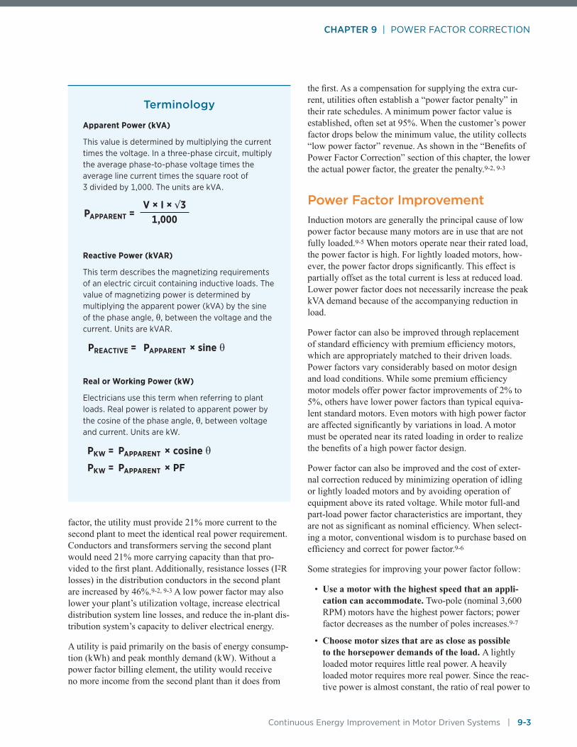
CHAPTER 9 | POWER FACTOR CORRECTION
Continuous Energy Improvement in Motor Driven Systems | 9-3
factor, the utility must provide 21% more current to the second plant to meet the identical real power requirement. Conductors and transformers serving the second plant would need 21% more carrying capacity than that pro-vided to the first plant. Additionally, resistance losses (I2R losses) in the distribution conductors in the second plant are increased by 46%.9-2, 9-3 A low power factor may also lower your plant’s utilization voltage, increase electrical distribution system line losses, and reduce the in-plant dis-tribution system’s capacity to deliver electrical energy.
A utility is paid primarily on the basis of energy consump-tion (kWh) and peak monthly demand (kW). Without a power factor billing element, the utility would receive no more income from the second plant than it does from
the first. As a compensation for supplying the extra cur-rent, utilities often establish a “power factor penalty” in their rate schedules. A minimum power factor value is established, often set at 95%. When the customer’s power factor drops below the minimum value, the utility collects “low power factor” revenue. As shown in the “Benefits of Power Factor Correction” section of this chapter, the lower the actual power factor, the greater the penalty.9-2, 9-3
Power Factor ImprovementInduction motors are generally the principal cause of low power factor because many motors are in use that are not fully loaded.9-5 When motors operate near their rated load, the power factor is high. For lightly loaded motors, how-ever, the power factor drops significantly. This effect is partially offset as the total current is less at reduced load. Lower power factor does not necessarily increase the peak kVA demand because of the accompanying reduction in load.
Power factor can also be improved through replacement of standard efficiency with premium efficiency motors, which are appropriately matched to their driven loads. Power factors vary considerably based on motor design and load conditions. While some premium efficiency motor models offer power factor improvements of 2% to 5%, others have lower power factors than typical equiva-lent standard motors. Even motors with high power factor are affected significantly by variations in load. A motor must be operated near its rated loading in order to realize the benefits of a high power factor design.
Power factor can also be improved and the cost of exter-nal correction reduced by minimizing operation of idling or lightly loaded motors and by avoiding operation of equipment above its rated voltage. While motor full-and part-load power factor characteristics are important, they are not as significant as nominal efficiency. When select-ing a motor, conventional wisdom is to purchase based on efficiency and correct for power factor.9-6
Some strategies for improving your power factor follow:
• Use a motor with the highest speed that an appli-cation can accommodate. Two-pole (nominal 3,600 RPM) motors have the highest power factors; power factor decreases as the number of poles increases.9-7
• Choose motor sizes that are as close as possible to the horsepower demands of the load. A lightly loaded motor requires little real power. A heavily loaded motor requires more real power. Since the reac-tive power is almost constant, the ratio of real power to
Terminology
Apparent Power (kVA)
This value is determined by multiplying the current times the voltage. In a three-phase circuit, multiply the average phase-to-phase voltage times the average line current times the square root of 3 divided by 1,000. The units are kVA.
PAPPARENT = V × I × √3
1,000
Reactive Power (kVAR)
This term describes the magnetizing requirements of an electric circuit containing inductive loads. The value of magnetizing power is determined by multiplying the apparent power (kVA) by the sine of the phase angle, θ, between the voltage and the current. Units are kVAR.
PREACTIVE = PAPPARENT × sine θ
Real or Working Power (kW)
Electricians use this term when referring to plant loads. Real power is related to apparent power by the cosine of the phase angle, θ, between voltage and current. Units are kW.
PKW = PAPPARENT × cosine θPKW = PAPPARENT × PF

CHAPTER 9 | POWER FACTOR CORRECTION
9-4 | Continuous Energy Improvement in Motor Driven Systems
apparent power varies with induction motor load, and power factor ranges from about 10% at no load to as high as 85% or more at full load.9-2, 9-3, 9-7 (see Figure 9-2). An oversized motor draws more reactive current at light load than a smaller motor draws at full load.
Low power factor results when motors are operated at less than full load. This often occurs in cyclic pro-cesses (such as circular saws, ball mills, conveyors, compressors, grinders, extruders, or punch presses) for which motors are sized for the “worst case” or heaviest load expected to be encountered. In these applications, the power factor varies from moment to moment. Examples of situations in which low power factors occur (from 30% to 50%) include a surface grinder performing a light cut, an unloaded rotary screw air compressor, and a circular saw spinning without cutting.9-1 The industries shown in Table 9-1 typically exhibit low power factors and do not fully use the incoming utility-supplied current.9-1, 9-8
• Add power factor correction capacitors to your in-plant distribution system. Low power factors can be corrected by installing external capacitors at the main plant service or at individual pieces of equipment. Power capacitors serve as leading reactive current generators and counter the lagging reactive current in the system. By providing reactive current, they reduce the total amount of current that your system must draw from the utility.9-1
Pow
er F
acto
r
Motor Load
100
90
80
70
60
50
40
30
20
10
0%0% 25% 50% 100%75%
kW
kVA
Power Factor without Capacitor
Power Factor with Capacitor
kVAr
Figure 9-2. Power Factor as a Function of Motor Load
Helpful Tip
To help you improve the power factor of motor-driven systems, the Bonneville Power Administration has produced an Industrial Power Factor Analysis Guidebook.9-8 The guidebook addresses the following topics:
■■ How to tell if your plant could benefit from capacitors
■■ How to select capacitor schemes to eliminate power factor penalties and minimize losses
■■ How to perform detailed plant surveys to collect sufficient data to determine where to put capacitors
■■ Why the power system must be built with extra capacity to supply power
■■ How reactive power contributes to additional losses
■■ How capacitors, synchronous machines, and static (adaptive) power compensators correct for power factor
■■ When to use switched versus fixed capacitors
■■ How and when capacitors contribute to harmonic distortion problems, and how to predict this
■■ How capacitors can fall prey to harmonics and switching transients, and what to do about it.
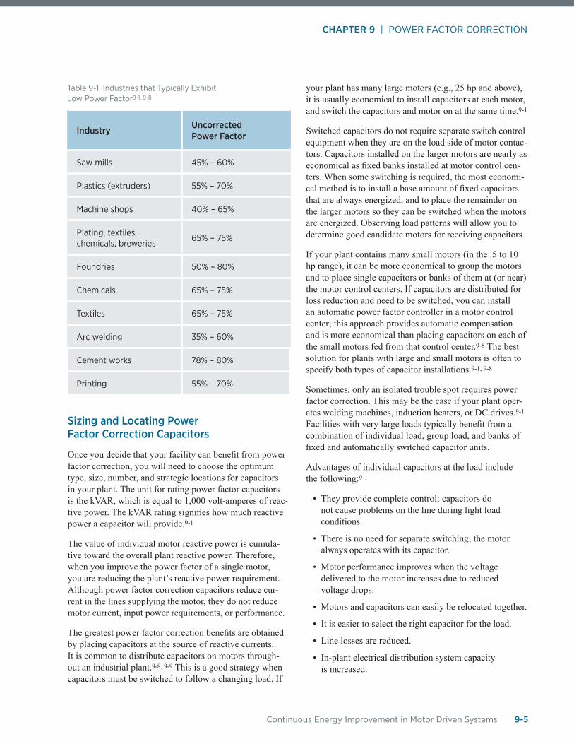
CHAPTER 9 | POWER FACTOR CORRECTION
Continuous Energy Improvement in Motor Driven Systems | 9-5
Sizing and Locating Power Factor Correction Capacitors
Once you decide that your facility can benefit from power factor correction, you will need to choose the optimum type, size, number, and strategic locations for capacitors in your plant. The unit for rating power factor capacitors is the kVAR, which is equal to 1,000 volt-amperes of reac-tive power. The kVAR rating signifies how much reactive power a capacitor will provide.9-1
The value of individual motor reactive power is cumula-tive toward the overall plant reactive power. Therefore, when you improve the power factor of a single motor, you are reducing the plant’s reactive power requirement. Although power factor correction capacitors reduce cur-rent in the lines supplying the motor, they do not reduce motor current, input power requirements, or performance.
The greatest power factor correction benefits are obtained by placing capacitors at the source of reactive currents. It is common to distribute capacitors on motors through-out an industrial plant.9-8, 9-9 This is a good strategy when capacitors must be switched to follow a changing load. If
your plant has many large motors (e.g., 25 hp and above), it is usually economical to install capacitors at each motor, and switch the capacitors and motor on at the same time.9-1
Switched capacitors do not require separate switch control equipment when they are on the load side of motor contac-tors. Capacitors installed on the larger motors are nearly as economical as fixed banks installed at motor control cen-ters. When some switching is required, the most economi-cal method is to install a base amount of fixed capacitors that are always energized, and to place the remainder on the larger motors so they can be switched when the motors are energized. Observing load patterns will allow you to determine good candidate motors for receiving capacitors.
If your plant contains many small motors (in the .5 to 10 hp range), it can be more economical to group the motors and to place single capacitors or banks of them at (or near) the motor control centers. If capacitors are distributed for loss reduction and need to be switched, you can install an automatic power factor controller in a motor control center; this approach provides automatic compensation and is more economical than placing capacitors on each of the small motors fed from that control center.9-8 The best solution for plants with large and small motors is often to specify both types of capacitor installations.9-1, 9-8
Sometimes, only an isolated trouble spot requires power factor correction. This may be the case if your plant oper-ates welding machines, induction heaters, or DC drives.9-1 Facilities with very large loads typically benefit from a combination of individual load, group load, and banks of fixed and automatically switched capacitor units.
Advantages of individual capacitors at the load include the following:9-1
• They provide complete control; capacitors do not cause problems on the line during light load conditions.
• There is no need for separate switching; the motor always operates with its capacitor.
• Motor performance improves when the voltage delivered to the motor increases due to reduced voltage drops.
• Motors and capacitors can easily be relocated together.
• It is easier to select the right capacitor for the load.
• Line losses are reduced.
• In-plant electrical distribution system capacity is increased.
Table 9-1. Industries that Typically Exhibit Low Power Factor9-1, 9-8
Industry Uncorrected Power Factor
Saw mills 45% – 60%
Plastics (extruders) 55% – 70%
Machine shops 40% – 65%
Plating, textiles, chemicals, breweries
65% – 75%
Foundries 50% – 80%
Chemicals 65% – 75%
Textiles 65% – 75%
Arc welding 35% – 60%
Cement works 78% – 80%
Printing 55% – 70%

CHAPTER 9 | POWER FACTOR CORRECTION
9-6 | Continuous Energy Improvement in Motor Driven Systems
The advantages of bank installations downstream of the utility meter at the plant substation or service entry include the following:9-1
• The cost per kVAR is lower.
• Installation costs are also lower.
• The total plant power factor improves, which reduces or eliminates utility power factor penalty charges.
• Total kVAR may be reduced because all capacitors are on line even when some motors are switched off.
• Automatic switching ensures the exact amount of power factor correction and eliminates over capaci-tance and resulting overvoltages.
If your facility operates at a constant load around the clock, fixed capacitors are the best solution. If the load is variable, such as two 7-hour production shifts, followed by a nighttime cleanup shift 5 days per week, you will need switched units to decrease capacitance during times of reduced load.9-1
If your feeders or transformers are overloaded, or if you wish to add additional load to already loaded lines, you should apply power factor correction at the load. If your facility has excess current-carrying capacity, you can install capacitor banks at main feeders.
There are three location options for installing capacitors at the motor, as indicated in Figure 9-3. These options, along with the types of motors applicable to each, are as follows:9-1
Location A — At the motor side of the overload relay
• New motor installations, in which overloads can be sized in accordance with a lower current draw
• Existing motors, when no overload change is required
Location B — Between the starter and overload relay
• Existing motors, when placement at location A would allow overload current to surpass code
Location C — At the line side of the starter
• Motors that are jogged or reversed (jogging refers to service conditions that include repeated starting and stopping of a motor such as moving a crane or a con-veyor to a particular location)
• Multispeed motors
• Starters with open transition, and those that discon-nect/reconnect the capacitor during cycle
• Motors that start frequently
• Motor loads with high inertia.
Sizing Capacitors for Individual Motors and Entire Plant LoadsCapacitors that are installed across the motor terminals and switched with the motor should not be sized larger than the amount of kVAR necessary to raise the motor no-load power factor to 100%.9-7 Use Table 9-2 to size capacitors for individual motor loads; look up the type of motor frame, synchronous speed (RPM), and horsepower.
Motor
MotorFeed
ThermalOverload
A B CFused Safety
Switch or Breaker
MotorStarter
CapacitorC
CapacitorB
CapacitorA
Figure 9-3. Locating Capacitors on Motor Circuits

CHAPTER 9 | POWER FACTOR CORRECTION
Continuous Energy Improvement in Motor Driven Systems | 9-7
The table indicates the kVAR necessary to correct the power factor to 95%.9-1
If you know the total plant load (kW), your present power factor, and the power factor you intend to achieve, you can use Table 9-3 to identify the required capacitance.9-1 This table is useful for sizing banks of capacitors that can be located at motor control centers, feeders, branch circuits, or the plant service entrance.
The power triangle in Figure 9-4 indicates the demands on a plant distribution system before and after adding capaci-tors to improve power factor. Increasing the power factor from 70% to 95% reduces the apparent power from 1,420 kVA to 1,050 kVA, a reduction of 26%.
1000 kW
1420 kVA Before
Cosine Ø =kW
———kVA
Cosine Ø1 = = 70% PF1000———1420
Cosine Ø2 = = 95% PF1000———1050
670 kVARCapacitor
Added
330 kVARAfter
1000 kVARBefore
1050 kVA After
Ø2Ø1
95% PFAfter
70%PF
Figure 9-4. Apparent Power Requirements Before and After Adding Power Factor Correction Capacitors
Table 9-2. Sizing Guide for Capacitors on Individual Motors9-1
NEMA Code
BC D
WoundRotor
Before 1955 U-Frame T-FramePoles 2 4 6 8 10 12 2 4 6 8 10 12 2 4 6 8 10 12 4-6 8 6
RPM 3,600 1,800 1,200 900 720 600 3,600 1,800 1,200 900 720 600 3,600 1,800 1,200 900 720 6001,800
1,200900 1,200
HP=3 1.5 1.5 1.5 2 2.5 3.5 1 1 1 2 1.5 1.5 2.5 3 3 4
5 2 2 2 3 4 4.5 1 2 2 2 2 2.5 3 4 4 5
7.5 2.5 2.5 3 4 5.5 6 1 2 4 4 2.5 3 4 5 5 6
10 3 3 3.5 5 6.5 7.5 2 2 4 5 5 5 4 4 5 6 7.5 8
15 4 4 5 6.5 8 9.5 4 4 4 5 5 5 5 5 6 7.5 8 19 5 5 5 5.5
20 5 5 6.5 7.5 9 12 4 5 5 5 10 10 6 6 7.5 9 10 12 5 6 6 7
25 6 6 7.5 9 11 14 5 5 5 5 10 10 7.5 7.5 8 10 12 18 6 6 6 7
30 7 7 9 10 12 16 5 5 5 10 10 10 8 8 10 14 15 23 7.5 9 10 11
40 9 9 11 12 15 20 5 10 10 10 10 15 12 13 16 18 23 25 10 12 12 13
50 12 11 13 15 19 24 5 10 10 15 15 20 15 18 20 23 24 30 12 15 15 18
60 14 14 15 18 22 27 10 10 10 15 20 25 18 21 23 26 30 35 18 18 18 20
75 17 16 18 21 26 33 15 15 15 20 25 30 20 23 25 28 33 40 19 23 23 25
100 22 21 25 27 33 40 15 20 25 25 40 45 23 30 30 35 40 45 27 27 30 33
125 27 26 30 33 40 48 20 25 30 30 45 45 25 36 35 42 45 50 35 38 38 40
150 33 30 35 38 48 53 25 30 30 40 45 50 30 42 40 53 53 60 38 45 45 50
200 40 38 43 48 60 65 35 40 60 55 55 60 35 50 50 65 68 90 45 60 60 65
250 50 45 53 58 70 78 40 40 60 80 60 100 40 60 63 82 88 100 54 70 70 75
300 58 53 60 65 80 88 45 45 80 80 80 120 45 68 70 100 100 120 65 90 75 85
350 65 60 68 75 88 95 60 70 80 80 50 75 90 120 120 135
400 70 65 75 85 95 105 60 80 80 160 75 80 100 130 140 150
450 75 68 80 93 100 110 70 100 80 90 120 140 160 160
500 78 73 83 98 108 115 70 100 120 150 160 180 180

CHAPTER 9 | POWER FACTOR CORRECTION
9-8 | Continuous Energy Improvement in Motor Driven Systems
Table 9-3. Multipliers to Determine Capacitor kVAR Required for Power Factor Correction9-1
Original Power Factor
Corrected Power Factor
0.80 0.81 0.82 0.83 0.84 0.85 0.86 0.87 0.88 0.89 0.90 0.91 0.92 0.93 0.94 0.95 0.96 0.99 1.0
0.50 0.982 1.008 1.034 1.060 1.086 1.112 1.139 1.165 1.192 1.220 1.248 1.276 1.306 1.337 1.369 1.403 1.440 1.589 1.732
0.51 0.937 0.962 0.989 1.015 1.041 1.067 1.094 1.120 1.147 1.175 1.203 1.231 1.261 1.292 1.324 1.358 1.395 1.544 1.6870.52 0.893 0.919 0.945 0.971 0.997 1.023 1.050 1.076 1.103 1.131 1.159 1.187 1.217 1.248 1.280 1.314 1.351 1.500 1.6430.53 0.850 0.876 0.902 0.928 0.954 0.980 1.007 1.033 1.060 1.088 1.116 1.144 1.174 1.205 1.237 1.271 1.308 1.457 1.6000.54 0.809 0.835 0.861 0.887 0.913 0.939 0.966 0.992 1.019 1.047 1.075 1.103 1.133 1.164 1.196 1.230 1.267 1.416 1.5590.55 0.769 0.795 0.821 0.847 0.873 0.899 0.926 0.952 0.979 1.007 1.035 1.063 1.093 1.124 1.156 1.190 1.227 1.376 1.519
0.56 0.730 0.756 0.782 0.808 0.834 0.860 0.887 0.913 0.940 0.968 0.996 1.024 1.054 1.085 1.117 1.151 1.188 1.337 1.4800.57 0.692 0.718 0.744 0.770 0.796 0.822 0.849 0.875 0.902 0.930 0.958 0.986 1.016 1.047 1.079 1.113 1.150 1.299 1.4800.58 0.655 0.681 0.707 0.733 0.759 0.785 0.812 0.838 0.865 0.893 0.921 0.949 0.979 1.010 1.042 1.076 1.113 1.262 1.4050.59 0.619 0.645 0.671 0.697 0.723 0.749 0.776 0.802 0.829 0.857 0.885 0.913 0.943 0.974 1.006 1.040 1.077 1.226 1.3690.60 0.583 0.609 0.635 0.661 0.687 0.713 0.740 0.766 0.793 0.821 0.849 0.877 0.907 0.938 0.970 1.004 1.041 1.190 1.333
0.61 0.549 0.575 0.601 0.627 0.653 0.679 0.706 0.732 0.759 0.787 0.815 0.843 0.873 0.904 0.936 0.970 1.007 1.156 1.2990.62 0.516 0.542 0.568 0.594 0.620 0.646 0.673 0.699 0.726 0.754 0.782 0.810 0.840 0.871 0.903 0.937 0.974 1.123 1.2660.63 0.483 0.509 0.535 0.561 0.587 0.613 0.640 0.666 0.693 0.721 0.749 0.777 0.807 0.838 0.870 0.904 0.941 1.090 1.2330.64 0.451 0.474 0.503 0.529 0.555 0.581 0.608 0.634 0.661 0.689 0.717 0.745 0.775 0.806 0.838 0.872 0.909 1.068 1.2010.65 0.419 0.445 0.471 0.497 0.523 0.549 0.576 0.602 0.629 0.657 0.685 0.713 0.743 0.774 0.806 0.840 0.877 1.026 1.169
0.66 0.388 0.414 0.440 0.466 0.492 0.518 0.545 0.571 0.598 0.626 0.654 0.682 0.712 0.743 0.775 0.809 0.846 0.995 1.1380.67 0.358 0.384 0.410 0.436 0.462 0.488 0.515 0.541 0.568 0.596 0.624 0.652 0.682 0.713 0.745 0.779 0.816 0.965 1.1080.68 0.328 0.354 0.380 0.406 0.432 0.458 0.485 0.511 0.538 0.566 0.594 0.622 0.652 0.683 0.715 0.749 0.786 0.935 1.0780.69 0.299 0.325 0.351 0.377 0.403 0.429 0.456 0.482 0.509 0.537 0.565 0.593 0.623 0.654 0.686 0.720 0.757 0.906 1.0490.70 0.270 0.296 0.322 0.348 0.374 0.400 0.427 0.453 0.480 0.508 0.536 0.564 0.594 0.625 0.657 0.691 0.728 0.877 1.020
0.71 0.242 0.268 0.294 0.320 0.346 0.372 0.399 0.425 0.452 0.480 0.508 0.536 0.566 0.597 0.629 0.663 0.700 0.849 0.9920.72 0.214 0.240 0.266 0.292 0.318 0.344 0.371 0.397 0.424 0.452 0.480 0.508 0.538 0.569 0.601 0.635 0.672 0.821 0.9640.73 0.186 0.212 0.238 0.264 0.290 0.316 0.343 0.369 0.396 0.424 0.452 0.480 0.510 0.541 0.573 0.607 0.644 0.793 0.9360.74 0.159 0.185 0.211 0.237 0.263 0.289 0.316 0.342 0.369 0.397 0.425 0.453 0.483 0.514 0.546 0.580 0.617 0.766 0.9090.75 0.132 0.158 0.184 0.210 0.236 0.262 0.289 0.315 0.342 0.370 0.398 0.426 0.456 0.487 0.519 0.553 0.590 0.739 0.882
0.76 0.105 0.131 0.157 0.183 0.209 0.235 0.262 0.288 0.315 0.343 0.371 0.399 0.429 0.460 0.492 0.526 0.563 0.712 0.8550.77 0.790 0.105 0.131 0.157 0.183 0.209 0.236 0.262 0.289 0.317 0.345 0.373 0.403 0.434 0.466 0.500 0.537 0.685 0.8290.78 0.052 0.078 0.104 0.130 0.156 0.182 0.209 0.235 0.262 0.290 0.318 0.346 0.376 0.407 0.439 0.473 0.510 0.659 0.8020.79 0.026 0.052 0.078 0.104 0.130 0.156 0.183 0.209 0.236 0.264 0.292 0.320 0.350 0.381 0.413 0.447 0.484 0.633 0.7760.80 0.000 0.026 0.052 0.078 0.104 0.130 0.157 0.183 0.210 0.238 0.266 0.294 0.324 0.355 0.387 0.421 0.458 0.609 0.750
0.81 0.000 0.026 0.052 0.078 0.104 0.131 0.157 0.184 0.212 0.240 0.268 0.298 0.329 0.361 0.395 0.432 0.581 0.7240.82 0.000 0.026 0.052 0.078 0.105 0.131 0.158 0.186 0.214 0.242 0.272 0.303 0.335 0.369 0.406 0.555 0.6980.83 0.000 0.026 0.052 0.079 0.105 0.132 0.160 0.188 0.216 0.246 0.277 0.309 0.343 0.380 0.529 0.6720.84 0.000 0.026 0.053 0.079 0.106 0.134 0.162 0.190 0.220 0.251 0.283 0.317 0.354 0.503 0.6460.85 0.000 0.027 0.053 0.080 0.108 0.136 0.164 0.194 0.225 0.257 0.291 0.328 0.477 0.620
0.86 0.000 0.026 0.053 0.081 0.109 0.137 0.167 0.198 0.230 0.264 0.301 0.450 0.5930.87 0.000 0.027 0.055 0.083 0.111 0.141 0.172 0.204 0.238 0.275 0.424 0.5670.88 0.000 0.028 0.056 0.084 0.114 0.145 0.177 0.211 0.248 0.397 0.5400.89 0.000 0.028 0.056 0.086 0.117 0.149 0.183 0.220 0.369 0.5120.90 0.000 0.028 0.058 0.089 0.121 0.155 0.192 0.341 0.484
0.91 0.000 0.030 0.061 0.093 0.127 0.164 0.313 0.4560.92 0.000 0.031 0.063 0.097 0.134 0.283 0.4260.93 0.000 0.032 0.066 0.103 0.252 0.3950.94 0.000 0.034 0.071 0.220 0.3630.95 0.000 0.037 0.186 0.329
0.96 0.000 0.149 0.2920.97 0.108 0.2510.98 0.060 0.2030.99 0.000 0.143
0.000
Instructions: 1. Find the present power factor in column. 2. Read across to optimum power factor column. 3. Multiply that number by kW demand. Example: If your plant consumed 410 kW, was currently operating at 73% power factor and you wanted to correct power factor to be 95% you would. 1. Find 0.73 in column. 2. Read across to 0.95 column. 3. Multiply 0.607 by 410 = 249 (round to 250.) 4. You need 250 kVAR to bring your plant to 95% power factor If you don’t know the existing power factor level of your plant, you will have to calculate it before using this table. To calculate existing power factor: kW divided by kVA = power factor.

CHAPTER 9 | POWER FACTOR CORRECTION
Continuous Energy Improvement in Motor Driven Systems | 9-9
Benefits of Power Factor CorrectionThe cost-effectiveness of power factor correction depends upon such variables as utility power factor penalties, the need for additional system capacity, energy and demand cost, hours of facility operation, distribution system wire sizes, and the distance between the motor and the electri-cal meter.9-10 As shown in the following examples, it is critical to understand your utility’s rate structure to assess the benefits or reduction in utility billing due to power fac-tor correction.9-1, 9-9
Secondary Benefits of Power Factor CorrectionExcessive line currents due to low power factors cause excessive in-plant distribution system voltage drops and increased resistance losses. Operating motor-driven equip-ment under low-voltage conditions results in decreased
efficiency, motor overheating, and diminished motor life. By adding power factor correction capacitors, you can restore operating voltage to proper design conditions.
When located at motor loads, power factor correction capacitors increase system current-carrying capacity, reduce voltage drops, and decrease distribution system resistance (I2R) losses.9-1 Increasing the power factor from 75% to 95% results in a 21% lower current in the conduc-tors serving the same kW load. By adding power factor correction capacitors at motor loads, you can increase the total kW loading served by the conductors without increasing line currents, wire size, transformer size, or facility kVA charges. By including power factor correction capacitors in new construction or facility expansions, you can reduce project costs through decreasing the sizes of transformers, cables, busses, and switches.9-1 In practice, however, current or ampacity ratings are a function of full-load equipment values; therefore, size reductions may be precluded by electrical codes.
Utility Rate Schedule
In this scenario, the utility charges according to kW demand ($4.50/kW) and includes a surcharge or adjustment for low power factor. The following formula shows a billing adjustment based upon a desired 95% power factor.
Plant Conditions
For our sample facility, the original demand is 4,600 kVA × 0.80, or 3,680 kW.
The multiplier applies to power factors up to 0.95.
Savings are $37,260/year.
Billing Before Power Factor Correction
3,680 kW × 0.95
0.80
= 4,370 × $4.50
= $19,665/month or $235,980/year
Billing After Power Factor Corrected to 95%
3,680 kW × 0.950.95
= 3,680 × $4.50
= $16,560/month or $198,720/year
kWBILLED = kWDEMAND ×0.95PF
Where:
kWBILLED = Adjusted or billable demand
kWDEMAND =Measured electric demand in kW
PF = Power factor as a decimal
Example 9-2

CHAPTER 9 | POWER FACTOR CORRECTION
9-10 | Continuous Energy Improvement in Motor Driven Systems
Utility Rate Schedule
The utility measures and bills based upon total current used (working plus reactive current) at $3.50/kVA demand.
Plant Conditions
Assume a constant 4,600 kVA demand with an 80% power factor. Correct to 95% power factor.
Savings are ($16,100–$13,555) × 12 months = $30,540/year.
Up to $61,000 could be spent on power factor correction equipment if plant management would support a 2-year simple payback on investment.
Billing Before Power Factor Correction
4,600 kVA × $3.50 = $16,000/month
Billing After Power Factor Corrected to 95%
kWDEMAND = kVADEMAND 1 × PF1
= 4,600 × 0.8 = 3,680
kWDEMAND 2 =kWDEMAND
PF2
kWDEMAND 2 =3,680
= 3,8730.95
Where:
kVA DEMAND 1 = kVA demand before PF correction
kVA DEMAND 2 = kVA demand after PF correction
kWDEMAND = Electric demand in kW
PF1 = Original power factor
PF2 = Power factor after correction
Corrected Billing: 3.873 kVA × $3.50 = $13,555/month
Example 9-3

CHAPTER 9 | POWER FACTOR CORRECTION
Continuous Energy Improvement in Motor Driven Systems | 9-11
Poor power factor contributes to power losses in the in-plant distribution system. Calculate the power loss by squaring the line current and multiplying by the circuit resistance (I2R). Generally, distribution system losses are small and are related to the cable length and inverse of the cross sectional area—a typical industrial plant will suf-fer only a 2% loss in the cables if they are loaded to full capacity.9-8 Reductions in losses (upstream of the power factor correction capacitor locations) are calculated by the relationship shown in Equation 9-2.9-1
The Industrial Electrical Distribution Systems Guidebook contains worksheets for calculating the benefits of correct-ing both individual motor and total plant power factor.9-14
Power Factor Correction CostsThe average cost for capacitors on a 480-volt system is about $30 to $40 per kVAR (not including installation costs). Automatic power factor controllers or capacitors with harmonic filters cost more. These features are typi-cally associated with capacitors exceeding 100 kVAR. A single large capacitor bank has a lower installed cost than multiple small installations scattered throughout the plant. The cost per kVAR for small capacitors on individual motors is substantially higher because of labor and materi-als costs. The cost of large banks is lower on a per-kVAR basis because of economies of scale. The installed cost per kVAR of capacitance is also lower at higher voltages. At medium voltage levels (2400 volts and up), unit costs are generally about $3 to $6 per kVAR.
% reduction = 100 − 100 × ( PF1 )2
PF2
Where:
% reduction =Percent reduction in distribution losses
PF1 = Original power factor
PF2 = Power factor after correction
Equation 9-2. Reduction in distribution system losses due to power factor correction at the motor or motor control center
Example 9-4
Assume that installing a power factor correction capacitor at a motor improves power factor from 85% to 95%. Losses are reduced by:
Loss Reduction = 100 − 100 × (85/95)2 or 19.9%
Remember that this is 19.9% of the losses only on the conductor used to serve the motor load. Also note that line losses are proportional to voltage drop. A drop from 480 volts at the transformer tap to 470 volts at the motor indicates a distribution system loss of (10/480) × 100 = 2.0%. Multiplying the loss reduction times the total distribution system losses gives a total energy savings of approximately 0.4% of the energy going down the conductor to serve the motor load.
Quick Fact
Short-circuit megavolt amperes (MVAs) represents system impedance. It is the current (in millions of amperes) that would be drawn by a short circuit, multiplied by the no-load voltage of the system at the point of interest. In reality, circuit protectors would blow before short-circuit current could stabilize, so it is defined by linearly extrapolating the volts-per-amp system voltage drop, at moderate load, down to zero system volts.
Helpful Tip
Beware of sales representatives claiming that their product will “reduce motor energy costs by up to 35%,” as benefits of “black boxes” are often greatly exaggerated.9-12 In reality, the product may reduce in-plant distribution system line losses by up to 35% (and only for the conductor serving an individual motor) or reduce the power supplied to an unloaded motor by up to 35%. Saving a large percentage of a small amount of energy or power may not result in significant or cost-effective dollar savings.9-13
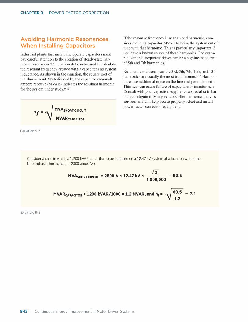
CHAPTER 9 | POWER FACTOR CORRECTION
9-12 | Continuous Energy Improvement in Motor Driven Systems
Avoiding Harmonic Resonances When Installing CapacitorsIndustrial plants that install and operate capacitors must pay careful attention to the creation of steady-state har-monic resonances.9-8 Equation 9-3 can be used to calculate the resonant frequency created with a capacitor and system inductance. As shown in the equation, the square root of the short-circuit MVA divided by the capacitor megavolt ampere reactive (MVAR) indicates the resultant harmonic for the system under study.9-15
If the resonant frequency is near an odd harmonic, con-sider reducing capacitor MVAR to bring the system out of tune with that harmonic. This is particularly important if you have a known source of these harmonics. For exam-ple, variable frequency drives can be a significant source of 5th and 7th harmonics.
Resonant conditions near the 3rd, 5th, 7th, 11th, and 13th harmonics are usually the most troublesome.9-15 Harmon-ics cause additional noise on the line and generate heat. This heat can cause failure of capacitors or transformers. Consult with your capacitor supplier or a specialist in har-monic mitigation. Many vendors offer harmonic analysis services and will help you to properly select and install power factor correction equipment.
Equation 9-3
MVASHORT CIRCUIT
MVARCAPACITOR
hƒ =
Consider a case in which a 1,200 kVAR capacitor to be installed on a 12.47 kV system at a location where the three-phase short-circuit is 2800 amps (A).
Example 9-5
MVASHORT CIRCUIT = 2800 A × 12.47 kV × 3
1,000,000= 60.5
MVARCAPACITOR = 1200 kVAR/1000 = 1.2 MVAR, and hf = 60.51.2
= 7.1

CHAPTER 9 | POWER FACTOR CORRECTION
Continuous Energy Improvement in Motor Driven Systems | 9-13
References 9-1 Eaton Corporation, “Power Factor Correction:
A Guide for the Plant Engineer,” Design it Right, Technical Data SA2607001E, November, 2010.
9-2 Carroll, Hatch & Associates, Inc., “An Electric Motor Energy Efficiency Guide and Technical Reference Manual,” June 1994.
9-3 Carroll, Hatch & Associates, Inc., “A Procedure for Developing an Energy Efficiency Plan for the Use of Electric Motors in an Industrial Setting,” June 1994.
9-4 “Reducing Power Factor Cost,” U.S. Department of Energy, Motor Challenge Program Fact Sheet, DOE/GO-10095-286, 1996.
9-5 Lobodovsky, K.K., “Power Factor Correction Capacitors – What – Why – Where – How,” Pacific Gas & Electric Technical Services Application Note No. 43-46-83.
9-6 Bonnett, Austin H., “Understanding Power Factor in Squirrel Cage Induction Motors,” U.S. Electrical Motors.
9-7 Ader, Edward and William Finley, “Compensating for Low Power Factor.” Plant Engineering, June 17, 1993.
9-8 “Industrial Power Factor Analysis Guidebook,” DOE/BP-42892-1, Bonneville Power Administration, April 1995.
9-9 Portland General Energy Systems, “Power Quality for Electrical Contractors: Application Guide,” Volume 7: Recommended Practices, Electric Power Research Institute, December 1994.
9-10 “Power Factor Correction Equals Big Savings,” Conserver, Georgia Tech Research Institute, March 1991.
9-11 Montgomery, Fred L., “The Dollars and Sense of Power Factor Correction,” AIPE Facilities Management, Operations & Engineering, September/October 1989.
9-12 Nailen, Richard L., “What does power factor ‘correction’ really mean?” Electrical Apparatus, July, 1997.
9-13 Nailen, Richard L., “How good are motor voltage controllers?” Electrical Apparatus, October, 1995.
9-14 Gray, Rob, Washington State Energy Office, “Keeping the Spark in Your Electrical System: An Industrial Electrical Distribution Systems Guidebook,” Funded by the Bonneville Power Administration, U.S. Department of Energy, Pacificorp, Portland General Electric and Tacoma City Light, October 1995.
9-15 PSI Energy, “Avoiding Steady-State Harmonic Resonances When Installing Capacitors,” Power Clinic Tech Tip, Issue Number 7.

Continuous Energy Improvement in Motor Driven Systems

APPENDICES
Continuous Energy Improvement in Motor Driven Systems | A-1
APPENDICES
Appendix A: Motor Nameplate and Field Test Data Form
Employee Name _________________________________________
Company ______________________________________________
Date __________________________________________________
General Data
Serving Electrical Utility ___________________________________
Energy Rate ($/kWh) _____________________________________
Monthly Demand Charge ($/kW/mo) _________________________
Application _____________________________________________
Type of equipment that motor drives
Coupling Type __________________________________________
Motor Type (Design A, B, C, D, AC, DC etc.) ____________________
Motor Purchase Date/Age __________________________________
Rewound Yes No
Motor Nameplate Data
1. Manufacturer _______________________________________
2. Motor ID Number ____________________________________
3. Model _____________________________________________
4. Serial Number ______________________________________
5. NEMA Design Type ___________________________________
6. Size (hp) __________________________________________
7. Enclosure Type ______________________________________
8. Synchronous Speed (RPM) _____________________________
9. Full Load Speed (RPM) ________________________________
10. Voltage Rating ______________________________________
11. Frame Designation ___________________________________
12. Full Load Amperage __________________________________
13. Full Load Power Factor (%) ____________________________
14. Full Load Efficiency (%) _______________________________
15. Service Factor Rating _________________________________
16. Temperature Rise ____________________________________
17. Insulation Class _____________________________________
18. kVA Code __________________________________________
Facility/Location _________________________________________
Department ____________________________________________
Process ________________________________________________
Motor Operating Profile
Weekdays _______________ Wknd/Holiday ________
Days/Year _______________ Days/Year ___________
1st Shift _________________ ___________________
2nd Shift ________________ ___________________
3rd Shift _________________ ___________________
Annual Operating Time____________hours/year
Type of load (Place an “X” by the most appropriate type)
______ 1. Load is quite steady, motor “On” during shift
______ 2. Load starts, stops, but is constant when “On”
______ 3. Load starts, stops, and fluctuates when “On”
Answer the following only if #2 or #3 above was selected:
% of time load is “on” _______%
Answer the following only if #3 was selected:
Estimate average load as a % of motor size _______%
Measured Data
Supply Voltage
By Voltmeter
Vab ______________
Vbc ______________ Vavg______________
Vca ______________
Input Amps
By Ampmeter
Aa ______________
Ab ______________ Aavg _____________
Ac ______________
Power Factor (PF, %) _____________________________________
Input Power (kW) _______________________________________
If available. Otherwise equal to: Vavg × Aavg × (PF/100) × √3/1000
Motor Operating Speed (RPM) ______________________________ By Tachometer
Driven Equipment Operating Speed (RPM) ____________________
HoursPerDay
Line-to-
Line-

APPENDICES
A-2 | Continuous Energy Improvement in Motor Driven Systems
Appendix B: Average Efficiencies for Standard Efficiency Motors at Various Load Points
Efficiencies for 900 RPM, Old Standard Efficiency Motors
Motor Size
Load Level In Percent
ODP TEFC
100% 75% 50% 25% 100% 75% 50% 25%
10 85.3 86.1 84.8 78.3 85.5 85.8 84.8 77.3
15 86.3 87.5 86.6 79.6 86.4 87.2 86.4 79.0
20 87.6 88.3 87.3 81.8 87.9 88.9 88.2 84.4
25 88.3 88.8 88.1 83.0 87.9 88.4 86.8 78.6
30 88.1 89.1 88.5 84.5 88.6 89.2 88.6 85.2
40 87.5 87.6 87.1 84.5 89.0 88.8 87.0 82.5
50 89.3 90.2 89.6 87.1 89.8 89.7 88.5 82.5
60 89.9 90.5 89.9 86.4 90.6 91.1 90.3 86.9
75 90.9 91.4 90.8 85.8 90.6 90.8 89.9 83.6
100 91.3 91.7 91.2 86.8 91.1 91.6 91.0 88.0
125 91.6 92.1 91.6 89.5 91.5 91.4 90.5 87.5
150 91.9 92.6 92.2 89.7 91.5 91.7 91.0 88.0
200 92.6 93.5 93.1 90.2 93.0 93.8 93.1 90.1
250 93.6 94.4 94.2 92.7 94.2 94.5 94.4 91.5
300 94.1 92.4 89.5 86.0 94.2 94.5 94.4 91.5

APPENDICES
Continuous Energy Improvement in Motor Driven Systems | A-3
Efficiencies for 1,200 RPM, Old Standard Efficiency Motors
Motor Size
Load Level In Percent
ODP TEFC
100% 75% 50% 25% 100% 75% 50% 25%
10 87.4 87.9 86.5 79.3 84.9 85.9 84.4 80.0
15 87.0 87.4 86.3 79.6 87.0 87.2 86.0 79.7
20 87.7 88.6 88.3 85.1 87.7 88.8 88.2 83.6
25 89.0 89.5 88.8 85.2 88.9 89.5 88.5 81.3
30 89.5 90.2 89.7 87.6 89.6 90.3 89.0 83.8
40 89.4 89.9 89.2 85.2 89.9 90.4 88.6 84.5
50 89.7 89.2 87.8 71.7 90.6 91.2 90.5 86.0
60 90.8 91.5 90.9 87.5 90.8 91.0 90.2 83.1
75 91.5 91.7 91.8 88.9 91.6 91.6 90.7 86.5
100 92.0 92.5 92.1 88.3 92.1 92.1 91.9 84.5
125 92.0 92.5 92.1 88.3 92.1 92.1 91.9 86.0
150 92.6 93.1 92.6 90.0 93.1 93.3 92.6 90.8
200 92.9 93.1 91.7 89.9 92.6 93.2 92.5 88.4
250 94.1 94.2 93.3 92.7 94.4 94.4 93.9 90.0
300 94.4 94.6 94.5 92.8 94.4 94.4 93.8 91.0

APPENDICES
A-4 | Continuous Energy Improvement in Motor Driven Systems
Efficiencies for 1,800 RPM, Old Standard Efficiency Motors
Motor Size
Load Level In Percent
ODP TEFC
100% 75% 50% 25% 100% 75% 50% 25%
10 86.1 87.4 86.9 81.8 85.7 86.7 85.4 77.4
15 87.8 88.8 88.3 82.0 86.6 87.5 86.0 74.9
20 88.3 89.4 88.7 83.3 88.5 89.3 88.5 82.9
25 88.9 90.0 89.8 86.6 89.3 89.9 88.8 82.1
30 88.9 90.6 90.5 87.4 89.6 90.2 89.2 83.6
40 90.0 90.3 89.4 85.7 90.2 90.4 89.2 81.6
50 90.7 91.2 90.4 87.4 91.3 91.6 90.9 84.1
60 91.3 91.7 90.8 86.8 91.8 91.9 90.8 85.2
75 91.9 92.3 91.6 87.7 91.7 92.0 90.9 85.1
100 92.1 92.7 92.2 89.2 92.3 92.2 91.2 86.2
125 92.2 92.8 92.2 88.2 92.2 91.6 90.5 84.0
150 92.8 93.1 92.4 88.6 93.0 92.8 91.5 86.3
200 93.0 93.4 93.0 90.3 93.5 93.3 92.0 86.3
250 94.4 94.6 93.8 92.0 94.2 94.1 93.0 88.8
300 94.6 94.7 93.8 92.8 94.4 94.2 93.1 89.9

APPENDICES
Continuous Energy Improvement in Motor Driven Systems | A-5
Efficiencies for 3,600 RPM, Old Standard Efficiency Motors
Motor Size
Load Level In Percent
ODP TEFC
100% 75% 50% 25% 100% 75% 50% 25%
10 85.0 86.1 85.0 78.7 85.0 84.7 82.7 74.1
15 86.6 87.7 86.8 80.5 85.7 85.8 83.6 73.2
20 88.1 88.9 88.8 85.4 86.6 87.7 86.1 76.7
25 88.4 89.2 88.7 83.7 87.5 87.4 85.3 75.2
30 87.7 88.9 88.8 84.7 87.7 87.0 84.7 75.4
40 88.6 89.7 899 86.9 88.5 88.0 85.8 75.2
50 89.1 90.1 89.8 88.4 89.0 88.7 86.7 77.8
60 90.4 90.9 90.9 87.8 89.4 88.4 85.8 76.6
75 90.4 90.6 90.1 85.7 90.6 89.9 88.0 78.9
100 90.5 91.2 91.0 89.0 90.9 90.3 88.7 81.9
125 91.2 91.9 91.4 90.3 90.9 90.1 87.9 77.4
150 91.7 91.8 91.9 90.1 91.5 90.9 88.4 81.7
200 91.5 91.7 90.9 83.6 92.7 92.0 90.1 83.5
250 93.0 93.0 92.8 87.4 94.7 94.7 93.8 91.0
300 93.9 94.3 93.5 90.6 94.7 94.4 93.5 89.8

APPENDICES
A-6 | Continuous Energy Improvement in Motor Driven Systems
Appendix C: Motor Energy Savings Calculation Form
Employee Name _________________________________________
Company ______________________________________________
Date __________________________________________________
Motor Nameplate and Operating Information
Manufacturer ___________________________________________
Motor ID Number ________________________________________
Size (hp) _______________________________________________
Enclosure Type __________________________________________
Synchronous Speed (RPM) ________________________________
Full Load Speed (RPM) ____________________________________
Full Load Amperage ______________________________________
Full Load Power Factor (%) _________________________________
Full Load Efficiency (%) ___________________________________
Utility Rates
Energy Rate ($/kWh) _____________________________________
Monthly Demand Charge ($/kW/mo.) _________________________
Annual Operating Hours (hrs./yr.) ____________________________
Annual Energy Use and Cost
Input Power (kW) _______________________________________
Annual Energy Use _______________________________________
Input Power × Annual Operating hours
Annual Energy Cost ______________________________________
Annual Energy Use × Energy Rate
Annual Demand Cost _____________________________________
Input Power × Monthly Demand Charge × 12
Total Annual Cost ________________________________________
Annual Energy Cost + Annual Demand Cost
Facility/Location _________________________________________
Department ____________________________________________
Process ________________________________________________
Motor Load and Efficiency Determination
Load __________________________________________________
Input Power (kW) / [Motor Size (hp) × 0.746/Efficiency at Full Load]
Motor Efficiency at Operating Load __________________________
(Interpolate from Appendix B)
Energy Savings and Value
kW saved ______________________________________________
Input Power − [Load × hp × 0.746/Efficiency of Replacement Motor
at Load Point]
kWh saved _____________________________________________
kW saved × Annual Operating Hours
Total Annual Savings
Total Annual Savings $ ____________________________________
(kW saved × 12 × Monthly Demand Charge) +
(kWh saved x Energy Rate)
Cost for Replacement Motor ________________________________
(or Incremental Cost for New Motor)
Simple Payback (years) ___________________________________
(Cost for Replacement Motor + Installation Charge − Utility Rebate) /
Total Annual Savings
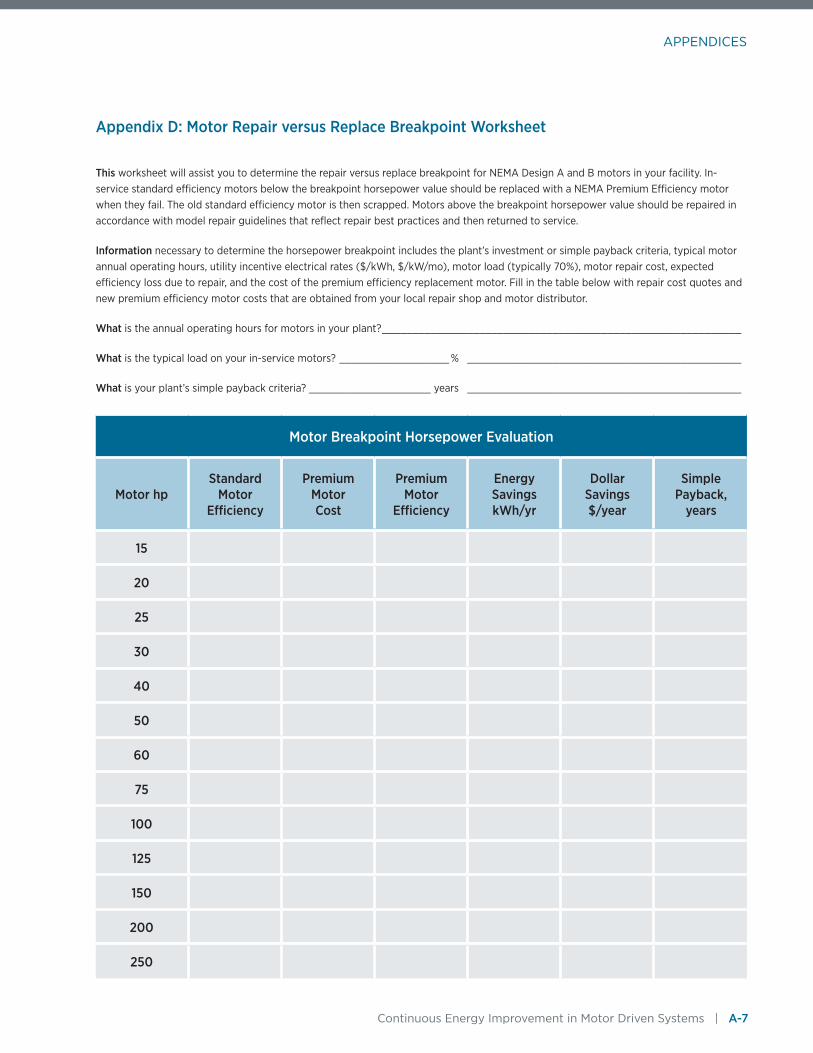
APPENDICES
Continuous Energy Improvement in Motor Driven Systems | A-7
Appendix D: Motor Repair versus Replace Breakpoint Worksheet
This worksheet will assist you to determine the repair versus replace breakpoint for NEMA Design A and B motors in your facility. In-service standard efficiency motors below the breakpoint horsepower value should be replaced with a NEMA Premium Efficiency motor when they fail. The old standard efficiency motor is then scrapped. Motors above the breakpoint horsepower value should be repaired in accordance with model repair guidelines that reflect repair best practices and then returned to service.
Information necessary to determine the horsepower breakpoint includes the plant’s investment or simple payback criteria, typical motor annual operating hours, utility incentive electrical rates ($/kWh, $/kW/mo), motor load (typically 70%), motor repair cost, expected efficiency loss due to repair, and the cost of the premium efficiency replacement motor. Fill in the table below with repair cost quotes and new premium efficiency motor costs that are obtained from your local repair shop and motor distributor.
What is the annual operating hours for motors in your plant? ___________________________________________________________
What is the typical load on your in-service motors? __________________ % _____________________________________________
What is your plant’s simple payback criteria? ____________________ years _____________________________________________
Motor Breakpoint Horsepower Evaluation
Motor hpStandard
Motor Efficiency
Premium Motor Cost
Premium Motor
Efficiency
Energy Savings kWh/yr
Dollar Savings $/year
Simple Payback,
years
15
20
25
30
40
50
60
75
100
125
150
200
250

Improving Steam System Performance: A Sourcebook for Industry, Second Edition One in a series of industrial energy efficiency sourcebooks.
DOE/GO-102014-4357 • February 2014
Printed with a renewable-source ink on paper containing at least 50% wastepaper, including 10% post consumer waste.
About the Office of Energy Efficiency and Renewable Energy The Office of Energy Efficiency and Renewable Energy (EERE) invests in clean energy technologies that strengthen the economy, protect the environment, and reduce dependence on foreign oil.
Advanced Manufacturing Office U.S. Department of Energy Energy Efficiency and Renewable EnergyWashington, D.C. 20585-0121
Co-sponsored by:
Copper Development Association260 Madison AvenueNew York, NY, USA 10016
Photo credits—page 1-1: iStock 6962363; page 2-1: Gates; page 3-1: David Parsons, NREL 05685 ; page 4-1: iStock 5219909; page 5-1: iStock 3667220; page 6-1: iStock 38353; page 7-1: iStock 15631110; page 8-1: Gates; page 9-1: iStock 8797738