continuous maneuvers for spacecraft formation flying
TRANSCRIPT

Acta Astronautica 153 (2018) 311–326
Contents lists available at ScienceDirect
Acta Astronautica
journal homepage: www.elsevier.com/locate/actaastro
Continuous maneuvers for spacecraft formation flying reconfiguration usingrelative orbit elements
G. Di Mauro a,*, R. Bevilacqua a,**, D. Spiller b, J. Sullivan c, S. D'Amico c
a Department of Mechanical and Aerospace Engineering, ADAMUS Laboratory, University of Florida, 939 Sweetwater Dr., Gainesville, FL 32611 – 6250, USAb Department of Mechanical and Aerospace Engineering, Sapienza University of Rome, via Eudossiana 18, 00184, Italyc Department of Aeronautics and Astronautics Engineering, Stanford Space Rendezvous Lab, Stanford University, 496 Lomita Mall, Stanford, CA 94305-4035, USA
A R T I C L E I N F O
Keywords:Spacecraft formation flying reconfigurationRelative orbit elementsRelative motion control
* Corresponding author.** Corresponding author.
E-mail addresses: [email protected] (G. Di Mau
https://doi.org/10.1016/j.actaastro.2018.01.043Received 3 August 2017; Received in revised form 14 JanAvailable online 2 March 20180094-5765/© 2018 The Authors. Published by Elsevier L
A B S T R A C T
This paper presents the solutions to the spacecraft relative trajectory reconfiguration problem when a continuousthrust profile is used, and the reference orbit is circular. Given a piecewise continuous thrust profile, the proposedapproach enables the computation of the control solution by inverting the linearized equations of relative motionparameterized using the mean relative orbit elements. The use of mean relative orbit elements facilitates theinclusion of the Earth's oblateness effects and offers an immediate insight into the relative motion geometry.Several reconfiguration maneuvers are presented to show the effectiveness of the obtained control scheme.
1. Introduction
Spacecraft formation flying concepts have become a topic of interestin recent years given the associated benefits in terms of cost, missionflexibility/robustness, and enhanced performance [1,2] Replacing acomplex, monolithic spacecraft with an array of simpler and highly co-ordinated satellites increases the performance of interferometric in-struments through the aperture synthesis. The configuration offormations can also be adjusted to compensate for malfunctioning vehi-cles without forcing a mission abort or be reconfigured to accomplishnew tasks.
Among the various technical challenges involved in spacecraft for-mation flying, the reconfiguration problem represents a key aspect thathas been intensively studied over the last years [2] Formation reconfi-guration pertains to the achievement of a specific relative orbit in adefined time interval given an initial formation configuration. So far,manymethods have been proposed to solve the aforementioned problem,ranging from impulsive to continuous control techniques. Impulsivestrategies have been widely investigated since they provide a closed-formsolution to the relative motion control problem. Such solutions aregenerally based on 1) the use of the Gauss variational equations (GVE) todetermine the control influence matrix, and 2) on the inversion of thestate transition matrix (STM) associated with a set of linear equations ofrelative motion. In Ref. [1] the authors addressed the issues of
ro), [email protected] (R. Bevilacqu
uary 2018; Accepted 23 January 201
td on behalf of IAA. This is an open a
establishing and reconfiguring a multi-spacecraft formation consisting ofa central chief satellite surrounded by four deputy spacecraft usingimpulsive control under the assumption of two-body orbital mechanics.They proposed an analytical two-impulse control scheme for transferringa deputy spacecraft from a given location in the initial configuration toany given final configuration using the GVE and a linear relative dy-namics model characterized in terms of nonsingular orbital elementdifferences. Ichimura and Ichikawa developed an analytical open-timeminimum fuel impulsive strategy associated with theHill-Clohessy-Wiltshire equations of relative motion. The approach in-volves three in-plane impulses to achieve the optimal in-plane reconfi-guration [2]. Chernick et al. addressed the computation of fuel-optimalcontrol solutions for formation reconfiguration using impulsive maneu-vers [3]. They developed semi-analytical solutions for in-plane andout-of-plane reconfigurations in near-circular J2-perturbed and eccentricunperturbed orbits, using the relative orbit elements (ROE) to parame-terize the equations of relative motion. More recently, Lawn et al. pro-posed a continuous low-thrust strategy based on the input-shapingtechnique for the short-distance planar spacecraft rephasing andrendezvous maneuvering problems [4]. The analytical solution was ob-tained by exploiting the Schweighart and Sedwick (SS) linear dynamicsmodel.
Additionally, the growing use of small spacecraft for formation flyingmissions poses new challenges for reconfiguration maneuvering. Due to
a).
8
ccess article under the CC BY license (http://creativecommons.org/licenses/by/4.0/).

G. Di Mauro et al. Acta Astronautica 153 (2018) 311–326
the vehicles' limited size, small spacecraft are typically equipped withsmall thrusters which only operate in continuous mode to deliver lowthrust. Many numerical methods have been investigated for the compu-tation of the minimum-fuel reconfiguration maneuver using continuouslow-thrust propulsion system. Steindorf et al. proposed a continuouscontrol strategy for formations operating in perturbed orbits of arbitraryeccentricity [5]. They derived a control law based on the Lyapunovtheory and ROE dynamics parameterization, and implemented guidancealgorithms based on potential fields. This approach allowed time con-straints, thrust level constraints, wall constraints, and passive collisionavoidance constraints to be included in the guidance strategy. Richardset al. proposed fuel-optimal control algorithm by using the lineartime-varying Hill–Clohessy–Wiltshire relative dynamics model. The tra-jectory optimization approach were based on the solution of amixed-integer linear programming (MILP) problem [6]. Huntington et al.developed a nonlinear fuel-optimal configuration method for tetrahedralformation based on Gauss variational equations. The associated optimi-zation problem is solved using Gauss pseudospectral method [7]. Massariet al. proposed a nonlinear low-thrust trajectory optimization methodusing a combination of parallel multiple shooting direct transcription anda barrier interior point method. They exploited a nonlinear dynamicsmodel to describe the relative motion considering any kind of positionalforce field [8].
Ultimately, future formation flying missions will need to operateautonomously to enhance the mission performance, increase the missionrobustness/flexibility, and reduce the overall costs. The achievement ofsuch on-board autonomy requires the development of formation controlalgorithms that are able to efficiently provide a solution on-boardwithout scarifying the maneuvering accuracy, [9].
In light of the above challenges, this work addresses the design of acomputationally efficient strategy for the reconfiguration of a formationin J2-perturbed near-circular orbits using a finite number of finite-timemaneuvers. The main contributions of this work are:
� the development of a linearized relative dynamics model and thederivation of the corresponding closed-form solution. In further de-tails, the results previously published in Ref. [10] are extended bycomputing the input matrix and the corresponding convolution ma-trix. In the framework of spacecraft relative motion, different dy-namics models have been developed over the years, based ondifferent state representation and subject to a multitude of constraintsand limitations on the intersatellite range of applicability, the ec-centricity of the satellite orbits, and the type of modeled perturbationforces, [11,12]. In this study the relative motion is parameterized interms of relative orbit elements (ROE) taking into account the J2perturbation and the control accelerations.
� the derivation of the analytical and semi-analytical control solutionsfor the in-plane and out-of-plane formation reconfiguration problems,respectively, using a continuous acceleration profile.
The rest of the paper is organized as follows. In the first section, thedifferential equations (and their associated linearization) describing therelative motion of two Earth orbiting spacecraft under the effects of J2and continuous external accelerations are presented. A closed-form so-lution for the linearized relative motion is derived for near-circular orbitcases, i.e. for very small or zero eccentricity. The subsequent section isdevoted to the derivation of control solutions for the in-plane, out-of-plane, and full spacecraft formation reconfiguration problems. Analyticaland numerical approaches are proposed to efficiently compute a feasiblereconfiguration maneuver. The final section shows the relative trajec-tories obtained using the developed control solutions, pointing out theirperformances in terms of maneuver cost and accuracy. In the same sec-tion a comparison with the minimum-fuel maneuver obtained using aglobal optimizer is also presented.
312
2. Relative dynamics model
In this section the dynamics model used to describe the relative mo-tion between two spacecraft orbiting the Earth is presented. The model isformalized by using the ROE state as defined by D'Amico in Refs. [13,14],and allows for the inclusion of Earth oblateness J2 and external constantacceleration effects.
2.1. Relative orbit elements
The absolute orbit of a satellite can be expressed by the set of classicalKeplerian orbit elements; α ¼ ½a; e; i;ω;Ω;M�T . The relative motion of adeputy spacecraft with respect to another one, referred to as chief, can beparameterized using the dimensionless relative orbit elements defined inRef. [13] and here recalled for completeness,
δα ¼
26666666666664
adac
� 1
ðMd �McÞ þ ðωd � ωcÞ þ ðΩd �ΩcÞcicex;d � ex;c
ey;d � ey;c
id � ic
ðΩd �ΩcÞsic
37777777777775¼
2666664δaδλδexδeyδixδiy
3777775 (1)
In Eq. (1) the subscripts “c” and “d” label the chief and deputy sat-ellites respectively, whereas sð�Þ ¼ sinð�Þ and cð�Þ ¼ cosð�Þ. Moreover,ex;ð�Þ ¼ eð�Þcωð�Þ and ey;ð�Þ ¼ eð�Þsωð�Þ are defined as the components of theeccentricity vector and ω is the argument of perigee. The first twocomponents of the relative state δα, are the relative semi-major axis, δa,and the relative mean longitude δλ, whereas the remaining componentsconstitute the coordinates of the relative eccentricity vector, δe, andrelative inclination vector, δi. It is worth remarking that the use of theROE parameterization facilitates the inclusion of perturbing accelera-tions, such as Earth oblateness J2 effects or atmospheric drag, into thedynamical model and offers an immediate insight into the relative mo-tion geometry [14]. In addition, the above relative state is non-singularfor circular orbits (ec ¼ 0), whereas it is still singular for strictly equa-torial orbits (ic ¼ 0).
2.2. Non-linear equations of relative motion
The averaged variations of mean ROE (i.e. without short- and long-periodic terms) caused by the Earth's oblateness J2 effects can bederived from the differentiation of chief and deputy mean classical ele-ments, αc ¼ ½ac; ec; ic;ωc;Ωc;Mc�T and αd ¼ ½ad; ed; id;ωd;Ωd;Md�Trespectively [15,16],
_αc;J2 ¼
2666664_ac_ec_ic_ωc_Ωc_Mc
3777775 ¼ Kc
266403x1Qc
�2cosðicÞηcPc
3775 _αd;J2 ¼
2666664_ad_ed_id_ωd_Ωd_Md
3777775 ¼ Kd
266403x1Qd
�2cosðidÞηdPd
3775 ;
(2)
where
Kj ¼ γnja2j η
4j
ηj ¼ffiffiffiffiffiffiffiffiffiffiffiffiffi1� e2j
qnj ¼
ffiffiffiffiffiμa3j
s
Qj ¼ 5 cos�ij�2 � 1 Pj ¼ 3 cos
�ij�2 � 1 γ ¼ 3
4J2R2
E
(3)
In Eq. (3) the subscript “j” stands for “c” and “d”. J2 indicates thesecond spherical harmonic of the Earth's geopotential, RE the Earth's

G. Di Mauro et al. Acta Astronautica 153 (2018) 311–326
equatorial radius and μ the Earth gravitational parameter. Computing thetime derivative of mean ROE as defined in Eq. (1) and substituting Eq. (2)yields
δ _αJ2 ¼
26666640�
_Md � _Mc
�þ ð _ωd � _ωcÞ þ�_Ωd � _Ωc
�cic
�edsωd_ωd þ ecsωc _ωc
þedcωd_ωd � eccωc _ωc
0�_Ωd � _Ωc
�sic
3777775 ¼ σJ2ðαc;αdÞ (4)
with
σJ2ðαc;αdÞ ¼
¼
26666640
ðηdPdKd � ηcPcKcÞ þ ðKdQd � KcQcÞ � 2ðKdcid � Kccic Þcic�ey;dKdQd þ ey;cKcQc
ex;dKdQd � ex;cKcQc
0�2ðKdcid � Kccic Þsic
3777775(5)
In this study only the deputy is assumed to be maneuverable andcapable of providing continuous thrust along x, y, and z directions of itsown Radial-Tangential-Normal (RTN) reference frame (also known asLocal Vertical Local Horizontal (LVLH)). The RTN frame consists oforthogonal basis vectors with x pointing along the deputy absolute radiusvector, z pointing along the angular momentum vector of the deputyabsolute orbit, and y ¼ z � x completing the triad and pointing in thealong-track direction. The change of mean ROE caused by a continuouscontrol acceleration vector f can be determined through the well-knownGauss variational equations (GVE) [17,18]. In fact, as widely discussed inRef. [18], the mean orbit elements can be reasonably approximated bythe corresponding osculating elements since the Jacobian of theosculating-to-mean transformation is approximately a 6x6 identity ma-trix, with the off-diagonal terms being of order J2 or smaller. In otherwords, the variations of osculating elements are directly reflected incorresponding mean orbit elements changes. In light of the above, thevariation of mean ROE induced by the external force is
δ _αF ¼
26666666666664
_adac
_Md þ _ωd þ _Ωdcic
_edcωd � edsωd_ωd
_edsωd þ edcωd_ωd
id_Ωdsic
37777777777775¼ σFðαd; f Þ ¼ ΓFðαdÞf ; (6)
where the control acceleration vector f is expressed in the deputy RTNframe components as f ¼ ½fx; fy ; fz�T . The individual terms of the controlinfluence matrix ΓF are reported in Appendix A.
The relative motion between the deputy and chief satellites is givenby adding the contributions from Keplerian gravity, the J2 perturbation,and the external force vector f . The final set of nonlinear differentialequations is
δ _α ¼
266666640
nd � nc0000
37777775þ σJ2ðαc;αdÞ þ σFðαd; f Þ ¼ ξðαc;αdðαc; δαÞ; f Þ: (7)
Note that the function ξðαc;αdðαc; δαÞ; f Þ can be reformulated in termsof αc and δα using the following identities [16],
313
ad ¼ acδaþ ac; ed ¼ffiffiffiffiffiffiffiffiffiffiffiffiffiffiffiffiffiffiffiffiffiffiffiffiffiffiffiffiffiffiffiffiffiffiffiffiffiffiffiffiffiffiffiffiffiffiffiffiffiffiffiffiffiffiffiffiffiffiffiffiffiðeccωc þ δexÞ2 þ
�ecsωc þ δey
�2q
id ¼ ic þ δix; Md ¼ Mc þ δλ� ðωd � ωcÞ � ðΩd �ΩcÞcicδixωd ¼ tan�1
�ecsωc þ δeyeccωc þ δex
�; Ωd ¼ Ωc þ δiy
sic
(8)
such that δ _α ¼ ξðαc;δα; f Þ.
2.3. Linearized equations of relative motion
In order to obtain the linearized equations of relative motion, δ _α inEq. (7) can be expanded about the chief orbit (i.e., δα ¼ 0 and f ¼ 0) tofirst order using a Taylor expansion,
δ _αðtÞ ¼ ∂ξ∂δα
�δα ¼ 0f ¼ 0
δαðtÞ þ ∂ξ∂f
�δα ¼ 0f ¼ 0
f ¼ AðαcðtÞÞ δαðtÞ þ BðαcðtÞÞf :
(9)
The matrices A and B represent the plant and input matrices,respectively. Under the assumption of near-circular chief orbit (i.e.,ec→0), these matrices are given by
ANC ¼
2666666666666666664
0 0 0 0 0 0
�Λc 0 0 0 �KcFcSc 0
0 0 0 �KcQc 0 0
0 0 KcQc 0 0 0
0 0 0 0 0 0
7KcSc2
0 0 0 2KcTc 0
3777777777777777775
; (10)
BNC ¼ 1ncac
2666666666664
0 2 0
�2 0 0
suc 2cuc 0
�cuc 2suc 0
0 0 cuc
0 0 suc
3777777777775; (11)
where uc ¼ ωc þMc denotes the mean argument of latitude of chief orbitand the following substitutions are applied for clarity
Fc ¼ 4þ 3ηc; Ec ¼ 1þ ηc; Sc ¼ sinð2icÞ;
Tc ¼ sinðicÞ2; Λc ¼ 32nc þ 7
2EcKcPc:
(12)
For an analysis of the applicability range of the linear relative dy-namics model (9)–(11) we address the reader to [14].
2.4. Analytical solution for near-circular linear dynamics model
The solution of the linear system (9), δαðtÞ; can be expressed as afunction of the initial ROE state vector δαðt0Þ, and the constant forcingvector, f , i.e. as
δαðtÞ ¼ Φðt; t0Þδαðt0Þ þ Ψ ðt; t0Þf (13)
where Φðt; t0Þ and Ψ ðt; t0Þ indicate the STM and the convolution matrix,respectively. As widely discussed in Refs. [10,16], Floquet theory can beexploited to derive the STM. The STM associatedwith near-circular linearrelative dynamics model is reported here for completeness
G. Di Mauro et al. Acta Astronautica 153 (2018) 311–326
6 1 0 0 0 0 07
ΦNCðt; t0Þ ¼2666666666664
�ΛcΔt 1 0 0 �KcFcScΔt 0
0 0 cΔω �sΔω 0 0
0 0 sΔω cΔω 0 0
0 0 0 0 1 072KcScΔt 0 0 0 2KcTcΔt 1
3777777777775
(14)
where Δt ¼ t � t0 and Δω ¼ KcQcΔt. According to linear dynamics sys-tem theory [19], the convolution matrix, Ψ ðt; t0Þ, can be computed bysolving the following integral,
ΨNCðt; t0Þ ¼ ∫ tt0ΦNCðt; τÞBNCðαcðτÞÞdτ (15)
Note that the integrand of the integral (15) does not include thecontrol vector since f is assumed to be constant over the interval ½t0; t�.Substituting the STM and the BNC matrices reported in Eqs. (14) and (10),respectively, into Eq. (15) yields
ΨNCðt ; t0Þ ¼
26666666666666666666666664
02Δu
ncacWc0
� 2ΔuncacWc
� ΛcΔu2
ncacW2c
ψ23
� cuc;t � cuc;0þCΔu
ncacð1� CÞWc2suc;t � suc;0þCΔu
ncacð1� CÞWc0
� suc;t � suc;0þCΔu
ncacð1� CÞWc�2
cuc;t � cuc;0þCΔu
ncacð1� CÞWc0
0 0suc;t � suc;0ncacWc
072KcScΔu2
ncacW2c
ψ63
37777777777777777777777775
(16)
ψ23 ¼FcKcSc
�cuc;t � cuc;0 þ suc;0Δu
�ncacW2
c
ψ63
¼��ðWc þ 2KcTcÞ
�cuc;t � cuc;0
�ncacW2
c
� 2KcTcsuc; 0Δu
ncacW2c
�
where uc;t and uc;0 are the mean argument of latitude of chief orbit at theinstant t and t0, respectively, and Δu ¼ uc;t � uc;0. In Eq. (16) the terms Cand Wc are constant coefficients that depend on the mean semi-majoraxis, eccentricity, and inclination of the chief orbit as follows
Wc ¼ nc þ KcQc þ ηcKcPc; C ¼ KcQc
Wc: (17)
314
Note that the mean argument of the latitude can be written as afunction of time using the relationships reported in Eq. (2), i.e., uc;t ¼uc;0 þ Wcðt� t0Þ.
3. Reconfiguration control problem
This section presents the derivation of a control solution for thereconfiguration problem, using a finite number of finite-time maneuvers.Recall that the trajectory reconfiguration problem denotes the achieve-ment of a certain user-defined set of ROE after a given time interval.Again, only the deputy is assumed to be maneuverable and capable ofproviding a piecewise continuous thrust along the x, y, and z directions ofits own RTN reference frame.
3.1. General approach
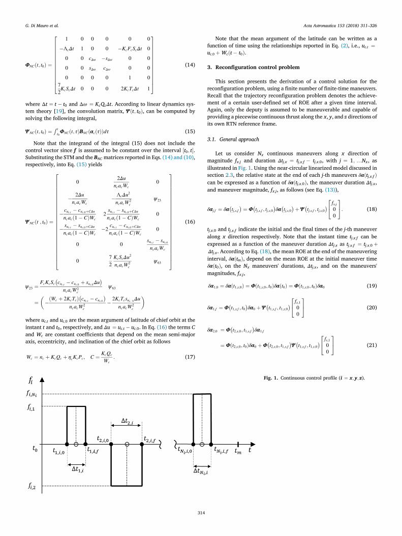
Let us consider Nx continuous maneuvers along x direction ofmagnitude fx;j and duration Δtj;x ¼ tj;x;f � tj;x;0, with j ¼ 1; …Nx, asillustrated in Fig. 1. Using the near-circular linearized model discussed insection 2.3, the relative state at the end of each j-th maneuvers δαðtj;x;f Þcan be expressed as a function of δαðtj;x;0Þ, the maneuver duration Δtj;x,and maneuver magnitude, fx;j, as follows (see Eq. (13)),
δαj;f ¼ δα�tj;x;f
� ¼ Φ�tj;x;f ; tj;x;0
�δα
�tj;x;0
�þ Ψ�tj;x;f ; tj;x;0
�24 fx;j00
35: (18)
tj;x;0 and tj;x;f indicate the initial and the final times of the j-th maneuveralong x direction respectively. Note that the instant time tj;x;f can beexpressed as a function of the maneuver duration Δtj;x as tj;x;f ¼ tj;x;0 þΔtj;x. According to Eq. (18), the mean ROE at the end of the maneuveringinterval, δαðtmÞ, depend on the mean ROE at the initial maneuver timeδαðt0Þ, on the Nx maneuvers' durations, Δtj;x, and on the maneuvers'magnitudes, fx;j,
δα1;0 ¼ δαðt1;x;0Þ ¼ Φðt1;x;0; t0Þδαðt0Þ ¼ Φðt1;x;0; t0Þδα0 (19)
δα1;f ¼ Φ�t1;x;f ; t0
�δα0 þ Ψ
�t1;x;f ; t1;x;0
�24 fx;100
35 (20)
δα2;0 ¼ Φ�t2;x;0; t1;x;f
�δα1;f
¼ Φðt2;x;0; t0Þδα0 þΦ�t2;x;0; t1;x;f
�Ψ�t1;x;f ; t1;x;0
�24 fx;100
35 (21)
Fig. 1. Continuous control profile (i ¼ x; y; z).

G. Di Mauro et al. Acta Astronautica 153 (2018) 311–326
δα2;f ¼ Φ�t2;x;f ; t2;x;0
�δα2;0 þ Ψ
�t2;x;f ; t2;x;0
�4 fx;20 5
203
¼ Φðt2;x;0; t0Þδα0 þ Φ�t2;x;f ; t1;x;f
�Ψ�t1;x;f ; t1;x;0
�24 fx;100
35þ Ψ�t2;x;f ; t2;x;0
�
�24 fx;2
00
35(22)
δαtm ¼ Φðtm; t0Þδα0 þXNx
j¼1
Φ�tm; tj;x;f
�Ψ�tj;x;f ; tj;x;0
�24 fx;j00
35: (23)
When the control thrust has a component along each RTN referenceframe axis, the change of mean ROE vector at the end of the maneuveringinterval is given by,
δαtm ¼ Φðtm; t0Þδα0 þ ςx þ ςy þ ςz (24)
where
ςx ¼XNx
j¼1
Φ�tm; tj;x;f
�Ψ�tj;x;f ; tj;x;0
�24 fx;j00
35ςy ¼
XNy
j¼1
Φ�tm; tj;y;f
�Ψ�tj;y;f ; tj;y;0
�24 0fy;j0
35ςz ¼
XNz
j¼1
þΦ�tm; tj;z;f
�Ψ�tj;z;f ; tj;z;0
�24 00fz;j
35:(25)
with ςi ¼�ςipiςoopi
�2 ℝ6, ςipi 2 ℝ4, ςoopi 2 ℝ2, and i ¼ x; y; z. The reconfi-
guration problem is described by the following expression
Δδαdes ¼ δαdes �Φðtm; t0Þδα0 ¼ ςx þ ςy þ ςz; (26)
where the term δαdes is the desired mean ROE vector at the end of themaneuvering interval. Eq. (26) represents a set of 6 nonlinear equationsin 3Nx þ 3Ny þ 3Nz unknowns, i.e. the maneuvers' magnitudes fi;j, theirapplication times, tj;i;0 (or alternatively the time of the middle point of themaneuver, i.e. ðtj;i;0 þ tj;i;f Þ=2), and the maneuvers' durations, Δtj;i, withi ¼ ; x; y; z. Note that the maneuvers-locations and durations will beexpressed in terms of mean argument of latitude throughout the paper,since the linear relationship that exists between the time and meanargument of latitude, i.e. uc;t ¼ uc;0 þ Wcðt� t0Þ. The vector δα0 isassumed to be known. According to Eq. (26), at least two maneuvers areneeded to obtain a finite number of analytical solutions.
In Ref. [3] the authors derived the semi-analytical solutions for thein-plane and out-of-plane reconfiguration problems in near-circularperturbed orbits using an impulsive maneuver scheme. This paper pre-sents the analytical and semi-analytical solutions for the same class ofproblems using continuous thrust maneuvers, and addresses the problemof full spacecraft formation reconfiguration. More specifically, thefollowing reconfiguration problems are considered:
� In-plane reconfiguration:
S1 ¼Δδbα ip
des ¼Δδades;Δδλdes;Δδex;des;Δδey;des
�T � Δδαdes
�;
� Out-of-plane reconfiguration:
S2 ¼Δδbαoop
des ¼Δδix;des;Δδiy;des
�T � Δδαdes
�;
315
� Full reconfiguration:
S3 ¼Δδbαfull
des ¼ ½Δδades;Δδλdes;Δδedes;Δδides�T�
The control solutions are obtained using the STM and convolutionmatrices associated with the near-circular dynamics model (see Eq. (14)and Eq. (16)).
3.2. In-plane reconfiguration
In this section the in-plane reconfiguration problem is addressed. Letus consider that only three tangential maneuvers are performed by thedeputy spacecraft fy;1, fy;2, and fy;3. This choice allows an analytical so-lution to be computed. Moreover, as discussed by Chernick et al. inRef. [3], the use of three tangential impulses allows finding a minimumdelta-V solution when the reconfiguration cost is driven by the variationof relative eccentricity vector. For this reason, the approach in this paperfocuses on a similar tangential maneuvering scheme.
According to Eq. (24), the equations governing the evolution of the in-plane mean ROE are
~u1;yfy;1 þ ~u2;yfy;2 þ ~u3;yfy;3 ¼ Wcncac4
Δδades (27)
��2Λc
�utm � bu1;y
�~u1;y
�fy;1 �
�2Λc
�utm � bu2;y
�~u2;y
�fy;2 �
�2Λc
�utm
� bu3;y
�~u3;y
�fy;3
¼ W2c ncac2
Δδλdes (28)
�cos
�Cutm þ ð1� CÞbu1;y
�sin
�ð1� CÞ~u1;y��fy;1 þ
�cos
�Cutm
þ ð1� CÞbu2;y
�sin
�ð1� CÞ~u2;y��fy;2 þ
�cos
�Cutm þ ð1� CÞbu3;y
�sin
��ð1� CÞ~u3;y
��fy;3
¼ ð1� CÞWcncac4
Δδex;des (29)
�sin
�Cutm þ ð1� CÞbu1;y
�sin
�ð1� CÞ~u1;y��fy;1 þ
�sin
�Cutm
þ ð1� CÞbu2;y
�sin
�ð1� CÞ~u2;y��fy;2 þ
�sin
�Cutm þ ð1� CÞbu3;y
�sin
��ð1� CÞ~u3;y
��fy;3
¼ ð1� CÞWcncac4
Δδey;des (30)
where
buj;y ¼ uj;f þ uj;02
~uj;y ¼ uj;f � uj;02
j ¼ 1;…3 (31)
and uj;0 and uj;f denote the chief mean argument of latitude at times tj;y;0and tj;y;f , respectively. Defining the variables
Uj;0;y ¼ ð1� CÞuj;0;y þ Cutm ; Uj;f ;y ¼ ð1� CÞuj;f ;y þ Cutm (32)
eUj;y ¼ Uj;f ;y � Uj;0;y
2¼ ð1� CÞ~uj;y j ¼ 1; ::; 3
bUj;y ¼ Uj;f ;y þ Uj;0;y
2¼ Cutm þ ð1� CÞbuj;y
(33)
allows for rearranging Eqs. (27)–(31) into a more convenient form, givenby
bU 1;yfy;1 þ eU2;yfy;2 þ eU3;yfy;3 ¼ ð1� CÞWcncac4
Δδades (34)

G. Di Mauro et al. Acta Astronautica 153 (2018) 311–326
��2Λc
�utm � bU 1;y
�~U1;y
�fy;1 �
�2Λc
�utm � bU 2;y
�~U2;y
�fy;2
��2Λc
�utm � bU 3;y
�~U3;y
�fy;3 ¼ ð1� CÞ2W2
c ncac2
Δδλdes (35)
�cos
bU 1;y
�sin
�eU1;y
��fy;1 þ
�cos
bU 2;y
�sin
�eU2;y
��fy;2
þ�cos
bU 3;y
�sin
�eU3;y
��fy;3
¼ ð1� CÞWcncac4
Δδex;des (36)
�sin
bU 1;y
�sin
�eU1;y
��fy;1 þ
�sin
bU 2;y
�sin
�eU2;y
��fy;2
þ�sin
bU 3;y
�sin
�eU3;y
��fy;3
¼ ð1� CÞWcncac4
Δδey;des (37)
It is worth noting that Eqs. (34)–(37) match the expressions obtainedfor three tangential impulses maneuver in Ref. [3]. Accordingly, the so-lution of the above system will have the same structure. In light of this,the locations (expressed as mean argument of latitude) of the maneuvermiddle points, buj;y , are given by
buj;y ¼bUj;y
1� C� Cutm1� C
j ¼ 1;…; 3
U ¼ atan�Δδey;desΔδex;des
�bU 1;y ¼ U þ k1π bU 2;y ¼ bU 1;y þ k2π bU 3;y ¼ bU 1;y þ k3π
(38)
where kj must be an integer number. The thrust magnitudes are
fy;j ¼ �nð�1Þk1 ð1� CÞWcacncΞj
oD
: (39)
where the quantities Ξj and D are detailed in Appendix B. It is worthremarking that the solution (38)–(39) is determined by assuming that the
maneuvers' locations, ~uj;y (or eUj;y) with j ¼ 1;…;3, are user-defined pa-rameters, i.e. by reducing the number of unknowns from 9 to 6. Other-wise, a numerical approach should be used to solve nonlinear system(38)–(39).
3.3. Out-of-plane reconfiguration
In this section the out-of-plane control solution is presented. In orderto achieve the desired x and y components of the relative inclinationvector at the end of the maneuver, the control solution must include acomponent in the cross-track (z) direction. In fact, the only way to modifythe difference in chief and deputy orbit inclination (i.e., δix) is to providea control acceleration along the z-axis of deputy RTN frame. This isimmediately evident from inspection of the linearized equations ofrelative motion (see Eq. (10)). If only a single cross-track maneuver isperformed by the deputy satellite, the equations governing the change ofrelative inclination vector are (see Eq. (24))
cosðbu1;zÞsinð~u1;zÞfz;1 ¼ Wcncac2
Δδix;des (40)
0@ 2KcTcðutm � bu1;z � ~u1;zÞcosðbu1;zÞsinð~u1;zÞþðWc þ 2KcTcÞsinðbu1;zÞsinð~u1;zÞ�2KcTc sinðbu1;z � ~u1;zÞ~u1;z
1Afz;1 ¼ W2c ncac2
Δδiy;des: (41)
The magnitude of the maneuver can be computed by inverting Eq.(40),
316
fz;1 ¼ Wcncac2½cosðbu1;zÞsinð~u1;zÞ�Δδix;des: (42)
If the maneuver duration, ~u1;z, is a user-defined parameter, the loca-tion of the maneuver, bu1;z, can be found by substituting Eq. (42) into Eq.(41) to obtain the following transcendental expression,
2KcTcðutm �bu1;z�~u1;zÞþ ðWcþ2KcTcÞtgðbu1;zÞ�2KcTc sinðbu1;z�~u1;zÞ~u1;zcosðbu1;zÞsinð~u1;zÞ
¼WcΔδiy;desΔδix;des
:
(43)
Eq. (43) can be numerically solved by using an iterative algorithmsuch as the bisection or Newton-Raphson methods [20]. In this study theBrent's method [20] implemented in fzero Matlab routine is used for thesolution of Eq. (43). The single out-of-plane maneuver solution for un-perturbed orbits provides useful insight into choosing a good initial guessfor quick convergence of the iterative approach. Alternatively, a para-metric analysis of the error function,
J ¼ 2KcTcðutm � bu1;z � ~u1;zÞ þ ðWc þ 2KcTcÞtgðbu1;zÞ
� 2KcTc sinðbu1;z � ~u1;zÞ~u1;zcosðbu1;zÞsinð~u1;zÞ �Wc
Δδiy;desΔδix;des
; (44)
is needed to determine the initial guess for the iterative algorithm.It is worth pointing out that, under the assumptions of using a single
finite-time maneuver with a given duration, the out-of-plane reconfigu-ration problem is reduced to the solution of a nonlinear equation (see Eq.(43)) for the determination of the maneuver location. In fact, the ma-neuver magnitude is analytically computed through the expression (42).It must be remarked, however, that the proposed approach only gua-rantees the achievement of the final desired relative configuration.
3.4. Full reconfiguration
In this section the solution of the full reconfiguration problem ispresented. Without loss of generality, the full reconfiguration is achievedthrough three tangential finite-time maneuvers and one single out-of-plane maneuver. At least one cross-track maneuver is needed to changethe relative inclination vector. Moreover, no radial maneuvers areconsidered since they are more demanding in terms of delta-V thantangential ones for the in-plane motion control, [13]. Assuming that themaneuvers' durations are user-defined parameters, the following set ofsix equations must be solved with respect to the unknowns magnitudesand locations, fy;j, fz;1, buj;y and bu1;z (j ¼ 1;…3), respectively
~u1;yfy;1 þ ~u2;yfy;2 þ ~u3;yfy;3 ¼ Wcncac4
Δδades (45)
��2Λc
�utm � bu1;y
�~u1;y
�fy;1 �
�2Λc
�utm � bu2;y
�~u2;y
�fy;2 �
�2Λc
�utm
� bu3;y
�~u3;y
�fy;3
þ FcKcSc
��sinðbu1;zÞsinð~u1;zÞ þ sinðbu1;z � ~u1;zÞ~u1;z þ ::::::� ðutm � bu1;z � ~u1;zÞcosðbu1;zÞsinð~u1;zÞ
�fz;1
¼ W2c ncac2
Δδλdes (46)
�cos
�Cutm þ ð1� CÞbu1;y
�sin
�ð1� CÞ~u1;y��fy;1 þ
�cos
�Cutm
þ ð1� CÞbu2;y
�sin
�ð1� CÞ~u2;y��fy;2 þ
�cos
�Cutm
þ ð1� CÞbu3;y
�sin
�ð1� CÞ~u3;y��fy;3
¼ ð1� CÞWcncac4
δex;des (47)

G. Di Mauro et al. Acta Astronautica 153 (2018) 311–326
sin Cutm þ ð1� CÞbu1;y sin ð1� CÞ~u1;y fy;1 þ sin Cutm� � �� � �
Table 1Initial mean chief orbit.
ac (km) ex (dim) ey (dim) ic (deg) Ωc (deg) uc (deg)
6578 0 0 8 0 0
� � � � �� � �þ ð1� CÞbu2;y sin ð1� CÞ~u2;y fy;2 þ sin Cutm
þ ð1� CÞbu3;y
�sin
�ð1� CÞ~u3;y��fy;3
¼ ð1� CÞWcncac4
Δδey;des (48)
cosðbu1;zÞsinð~u1;zÞfz;1 ¼ Wcncac2
Δδix;des (49)
�7KcSc
�utm � bu1;y
�~u1;y
�fy;1 þ
�7KcSc
�utm � bu2;y
�~u2;y
�fy;2 þ
�7KcSc
�utm
� bu3;y
�~u3;y
�fy;3 þ
0@ 2KcTcðutm � bu1;z � ~u1;zÞcosðbu1;zÞsinð~u1;zÞþþðWc þ 2KcTcÞsinðbu1;zÞsinð~u1;zÞþ
�2KcTc sinðbu1;z � ~u1;zÞ~u1;z
1Afz;1
¼ W2c ncac2
Δδiy;des (50)
The system (45)–(50) of 6 equations in 8 unknowns can be solvednumerically using a nonlinear least-squares problemmethod [21]. In thiswork, the Levenberg-Marquardt algorithm [22] implemented in thefsolveMatlab routine is used. Note that the proposed numerical approachonly guarantees the achievement of the desired relative configuration ina computationally efficient way. However, it does not enable the mini-mization of the fuel consumption. Ultimately, it is worth remarking thatthe obtained solution takes into account the dynamics coupling betweenthe in-plane and out-of-plane motion.
4. Numerical validation of the control solutions
In this section the relative trajectories obtained using the developedcontrol solutions are presented, pointing out their performances in termsof maneuver cost and accuracy. Fig. 2 illustrates the simulation setupexploited for the validation of the proposed maneuvering solutions.
First, the initial mean orbit elements of the chief and the mean ROEstate are set. Then, the initial mean orbit elements of the deputy arecomputed using the identities in Eq. (8). A numerical propagatorincluding the Earth's oblateness J2 effects is used to obtain the history ofposition and velocity of chief and deputy spacecraft expressed in EarthCentered Inertial (ECI) reference frame (J2000). The initial Cartesianstate of both satellites are derived using the linear mapping developed byBrouwer and Lyddane to transform the mean orbit elements into oscu-lating and the nonlinear relations between Cartesian state and osculatingelements [23–25]. The control thrust profile is projected into the ECIframe and added as external accelerations to the deputy's motion. Notethat 100 (kg) class of spacecraft are considered in this work, equippedwith cold gas propulsion system [26] for the relative maneuvering. Afterthe simulation, the absolute position and velocity of the spacecraft areconverted into the mean orbit elements to compute the accuracy at theend of the maneuvering interval, defined as
εδαk ¼��δαnum
k ðtmÞ � δαk;des
��acðt0Þ k ¼ 1;…; 6: (51)
In order to verify the effectiveness of the continuous thrust maneuversdiscussed in section 3, three test cases are carried out, involving the in-plane, out-of-plane, and full reconfiguration maneuvers defined in
317
section 3.1. Moreover, a comparison with the corresponding impulsivecontrol scheme reported in Ref. [3] is presented for in-plane andout-of-plane reconfiguration problems. A numerical optimizer is alsoused to verify the cost efficiency of the proposed solutions. However, itmust be said that a detailed study of the optimality of the solution is notcarried out in the frame of this work. The following minimum-fuelreconfiguration problems are investigated in the next sections:
� In-plane minimum-fuel reconfiguration. Find fj;y , ~uj;y and buj;y with j ¼ 1;
…;Ny that minimize ΔvTOT ¼ PNyj¼12fy;j~uj;y=Wc subject to
Δδbαipdes ¼ ςipy��fy;j�� < f ipmax; bujþ1;y > buj;y;
��~ujþ1;y þ ~uj;y�� < ��bujþ1;y � buj;y
�� : (52)
� Out-of-plane minimum-fuel reconfiguration. Find fj;z, ~uj;z and buj;z that
minimize ΔvTOT ¼ PNzj¼12fz;j~uj;z=Wc subject to
Δδbαoopdes ¼ ςoopz��fz;j�� < f oopmax ; bujþ1;z > buj;z;
��~ujþ1;z þ ~uj;z�� < ��bujþ1;z � buj;z
�� : (53)
� Full minimum-fuel reconfiguration. Find fj;y , ~uj;y and buj;y with j ¼ 1;…;
Ny , and fj;z, ~uj;z and buj;z that minimize ΔvTOT ¼ PNyj¼12fy;j~uj;y=Wc þPNz
j¼12fz;j~uj;z=Wc subject to
Δδbαfulldes ¼ ςy þ ςz��fy;j�� < f fullmax; bujþ1;y > buj;y;
��~ujþ1;y þ ~uj;y�� < ��bujþ1;y � buj;y
����fz;j�� < f fullmax; bujþ1;z > buj;z;��~ujþ1;z þ ~uj;z
�� < ��bujþ1;z � buj;z
�� : (54)
where the term fmax in Eqs. (52)–(54) denotes the maximum availableacceleration at the beginning of the maneuvering interval and rangesfrom 5x10�4 (m/s2) for the in-plane simulated scenario to 5x10�3 (m/s2)for the out-of-plane and full test cases. In this study, the global optimizerMultiStart provided by the Global Optimization Toolbox [27] is exploitedto solve the above optimization problems. MultiStart implements sto-chastic search methods to find the global minimum. It uses multiplerandom start points (including the user-defined initial guess) to samplemultiple basins of attraction and starts a local solver, such as fmincon,from those starting points, [28]. In the presented test cases 400 startpoints are used.
4.1. In-plane reconfiguration control problem
This section presents the trajectories obtained using the analytical
Fig. 2. Numerical validation scheme.

Table 2Initial and desired relative orbit.
acδa(m)
acδλ (m) acδex(m)
acδey(m)
acδix(m)
acδiy(m)
Initial relativeorbit, δα0
30 � 11e3 0 � 50 0 0
Desired relativeorbit, δαdes
0 �10:5e3
45 70 – –
Fig. 3. Control profile for in-plane maneuver.
G. Di Mauro et al. Acta Astronautica 153 (2018) 311–326
control solution reported in Eqs. (38) and (39) and the numerical solutiongiven by MultiStart solver. The initial conditions used in the simulationsare listed in Tables 1 and 2 (see first row), along with the desired meanROE vector. The initial mean state is expressed in terms of quasi-nonsingular orbital elements [17] in Table 1. Note that the values ofδα0 and δαdes lead to
acΔδbαdes ¼ ac
2664ΔδadesΔδλdesΔδex;desΔδey;des
3775 ¼ ½ � 0:03; 1:9172; 0:0403; 0:1198�T ðkmÞ: (55)
The reconfiguration maneuver lasts 5 orbits, i.e. uf ¼ 10π (rad),corresponding to tm ¼ 439:92 (min). In this simulation a maximum ac-celeration of 5e� 4 (m/s2) is considered, compatible with the maximumthrust provided by the cold gas propulsion system [26]. The analyticalsolution is obtained by choosing the parameters k ¼ ½k1; k2; k3� ¼ ½0; 1;6�(see Eq. (38)), corresponding to the maneuvers' locations, bUj;y , listed inTable 3. This choice derive from the analysis conducted in Ref. [3],wherein an impulsive solution is computed considering three tangentialimpulses placed at the same instants. In addition, the analytical solutionis computed assuming the maneuvers durations Δty ¼ ½11:01; 22:02;22:02� (min), corresponding to ~u1;y ¼ π=4 (rad) and ~u2;y ¼ ~u2;y ¼ π=2(rad). The maneuvers' magnitudes given by Eq. (39) are fy;1 ¼1:865 x 10�5 (m/s2), fy;2 ¼ �3:774 x 10�5 (m/s2), and fy;3 ¼1:499 x 10�5 (m/s2) (see Fig. 3), corresponding to a total delta-V of0:0820 (m/s). As discussed in previous section, the MultiStart solver al-lows the computation of the maneuvers' magnitudes, locations, and du-rations that minimize the total delta-V. As illustrated in Fig. 3 andconfirmed by the results reported in Table 3, the numerical approachbased on the global optimizer MultiStart reduces the maneuvers' dura-tions and increases the maneuvers' magnitudes in order to decrease thefuel consumption. In further details, the MultiStart algorithm provides acontrol profile consisting of three maneuvers of magnitude f MS
y;1 ¼ �2:62 x 10�4 (m/s2), fMS
y;2 ¼ 3:563 x 10�4 (m/s2), and f MSy;3 ¼ 4:509 x 10�4
(m/s2) and duration ΔtMSy ¼ ½2:94; 0:48; 0:67� (min), with a total ma-
neuver cost of about 0:0749 m/s (ΔvMSTOT ¼ 0:07489 (m/s)). In other
words, the MultiStart solution tends to the impulsive optimal one,decreasing the maneuver delta-V of 8.6% with respect to the analytical
Table 3Comparison between the analytical and numerical control solution for the in-plane maneuver.
Man. Loc.bUj;y
(rad)Δvj;y (m/s) ΔvTOT (m/
s)
Analytical Continuous Solution24 1:245
4:3820:09
35 24 0:0123�0:04980:0198
35 0:0820
Numerical Continuous Solution(MultiStart)
24 10:6720:1426:34
35 24 �0:04630:01020:0182
35 0:0749
Analytical Impulsive Solution([3])
24 1:2454:3820:09
35 24 0:0092�0:04630:0194
35 0:0748
318
solution). It must be pointed out that the MultiStart approach providesbetter performance in terms of maneuver cost even when the maneuvers'durations are constrained to be equal to those chosen for the computationof the analytical solution, i.e. ΔtMS
y ¼ Δty ¼ ½11:01;22:02;22:02� (min). Inthis case, the MultiStart method provides a reconfiguration strategyrequiring a delta-V of 0:0791 m/s (about the 3.5% lower than the delta-Vrequired by the analytical solution), and consisting of three maneuvers ofmagnitude f MS
y;1 ¼ �0:7331 x 10�4 (m/s2), f MSy;2 ¼ 0:1628 x 10�4 (m/s2),
and f MSy;3 ¼ 0:0694 x 10�4 (m/s2) placed at bU1;y ¼ 4:356 (rad), bU2;y ¼
7:5937 (rad), and bU3;y ¼ 26:4049 (rad).Figs. 4 and 5 illustrate the mean relative semi-major axis and longi-
tude, and the x- and y-component of mean relative eccentricity vectorrespectively. Both osculating and mean ROE are shown in the same plots.From these figures, both analytical and minimum-fuel continuous controlsolutions guarantee the achievement of the desired in-plane conditions inthe given interval of 5 orbits.
Table 4 shows the accuracy for the in-plane reconfiguration maneu-vers, i.e. the difference between the mean ROE at the end of the ma-neuver, tm, as computed by the numerical propagator, and the desiredROE multiplied by the chief mean-semi-major axis (see Eq. (51)). Thefinal error is at the meter level and is mainly due to the approximationsintroduced by the osculating-to-mean transformation at the end of thesimulations.
Ultimately, Fig. 6 shows the evolution of relative position in along-track/cross-track plane of chief RTN frame. In the same figure thefinite-time maneuvers are depicted (see green markers). The initial andthe desired relative positions are indicated by the cyan and blackmarkers, respectively.
4.2. Out-of-plane reconfiguration control problem
Here, the relative motion given by the cross-track maneuver pre-sented in section 3.3 is shown. In this scenario, a maneuver lasting 7orbits is considered, corresponding to tm ¼ 655:2 (min). The initial anddesired states listed in Tables 5 and 6 are used to run the verificationsimulations. The values of δα0 and δαdes yield the following change ofROE
acΔδbαdes ¼ ac
�Δδix;desΔδiy;des
�¼ ½0:3950; 0:0497�TðkmÞ: (56)
Eq. (43) is solved using the Brent's method [20] implemented in fzero

Fig. 4. Relative mean semi-major axis and longitudedue to in-plane reconfiguration maneuver.
Fig. 5. x- and y-component of mean relative eccen-tricity vector due to in-plane reconfigurationmaneuver.
Table 4Accuracy of control solutions for in-plane maneuver.
εδa (m) εδλ (m) εδex (m) εδey (m)
Analytical Continuous Solution 0:0449 2:182 0:197 0:034Numerical Continuous Solution 0:0451 2:187 0:192 0:035
G. Di Mauro et al. Acta Astronautica 153 (2018) 311–326
Matlab routine (referred to as semi-analytical continuous solution fromnow on). It is worth remarking that a parametric analysis of the errorfunction, J (see Eq. (44)), is carried out to determine a good initial guess
319
for the “fzero” solver. Differently, the author of [3] used the closed-formcontrol solution for unperturbed orbit as initial guess for the iterativealgorithm, i.e. bu1;z ¼ atanðΔiy;des=Δix;desÞ. The semi-analytical solution iscomputed setting a maneuver duration of about 23 (min) (correspondingto ~u1;z ¼ π=2 (rad)) and provides a control profile made of a maneuver ofmagnitude fz;1 ¼ 3:505 x 10�4 (m/s2) located at bu1;z ¼ 12:649 (rad) (seeTable 7), corresponding to a total delta-V of 0:492 m/s. The Brent's al-gorithm converges after 8 iterations. Table 7 shows also the maneuverlocation and the delta-V associated to the continuous solution given bythe MultiStart solver and to the semi-analytical impulsive solutioncomputed in Ref. [3]. The numerical approach based on the MultiStarttends to decrease the maneuver duration and increase the magnitude.

Fig. 6. Relative orbit projected on x-y plane of chiefRTN frame.
Table 5Initial mean chief orbit.
ac (km) ex (dim) ey (dim) ic (deg) Ωc (deg) uc (deg)
6828 0 0 78 0 0
Table 6Initial and desired relative orbit.
acδa(m)
acδλ(m)
acδex(m)
acδey(m)
acδix(m)
acδiy(m)
Initial relative orbit, δα0 0 0 0 � 50 5 70Desired relative orbit,δαdes
– – – – 400 120
Table 7Comparison between the semi-analytical and numerical control solutions for theout-of-plane maneuver.
Man. Loc. bu1;z
(rad)Δv1;z (m/s)
ΔvTOT (m/s)
Semi-analytical Continuous Solution(fzero)
12:649 0:492 0:492
Numerical Continuous Solution(MultiStart)
0:0661 0:443 0:443
Semi-analytical Impulsive Solution([3])
0:1275 0:443 0:443
Fig. 7. Control profile for out-of-plane maneuver.
G. Di Mauro et al. Acta Astronautica 153 (2018) 311–326
More specifically, the MultiStart solver gives an extremal solution, i.e.f MSz;1 ¼ fmax ¼ 5 x 10�3 (m/s2), consisting of a maneuver of 1:47 (min)located at the beginning of the maneuvering interval (see Fig. 7). Notethat the continuous semi-analytical solution is employed to initialize theMultiStart optimizer in this simulation. As expected, the MultiStartmethod reduces the total maneuver delta-V with respect to the
320
semi-analytical solution of about 12%, achieving the fuel consumptionobtained by the optimal impulsive solution (see Table 7). However, whenthe maneuver duration is constrained to be equal to 23 (min), i.e. to thevalue set for the computation of the semi-analytical solution, the Multi-Start solver does not provide an improvement in terms of delta-V, i.e.ΔvMS
TOT ¼ 0:492 (m/s), even though the cross-track maneuver has adifferent position and magnitude (f MS
z;1 ¼ �3:5019 x 10�4 (m/s2) andbuMS1;z ¼ 3:2119 (rad)).Fig. 8 shows the change of mean and osculating relative vector over
the maneuvering interval. Accordingly, both the continuous semi-analytical solution and the numerical one given by the MultiStart solverallow the achievement of the desired formation configuration within the7 orbits maneuvering interval. Table 8 reports the accuracy at the end ofthe maneuvering interval for the designed out-of-plane maneuver. Here,

Fig. 8. x- and y-component of mean relative inclination vector due to out-of-plane maneuver.
Table 8Accuracy of the control solutions for the out-of-plane maneuver.
εδix (m) εδiy (m)
Semi-analytical Continuous Solution (fzero) 0:3014 0:0134Numerical Continuous Solution (MultiStart) 0:3555 0:0165
Table 9Initial mean chief orbit.
ac (km) ex (dim) ey (dim) ic (deg) Ωc (deg) uc (deg)
6578 0 0 20 0 0
Table 10Initial and desired relative orbit.
acδa(m)
acδλ(m)
acδex(m)
acδey(m)
acδix(m)
acδiy(m)
Initial relative orbit, δα0 30 � 11e3 0 � 0:05 5 70Desired relative orbit,δαdes
0 �10:5e3
45 70 400 120
G. Di Mauro et al. Acta Astronautica 153 (2018) 311–326
the final error is at the centimeter level at most.Fig. 9 illustrates the trajectory projected on the cross-track/radial
plane of the chief RTN reference frame, along with its location. Theinitial and the aimed relative positions are indicated by the cyan andblack markers, respectively.
4.3. Full reconfiguration control problem
In this section the full reconfiguration results are discussed. Here, a
321
maneuver interval of 7 orbits is considered, i.e. uf ¼ 14π (rad). Tables 9and 10 report the initial and desired mean ROE respectively. In thisscenario, a simple analytical solution cannot be computed, as discussed insection 3.4. Consequently, the Matlab built-in routine fsolve is used toderive the continuous control solution, i.e. to solve the nonlinear systemof equations (45–(50) with respect to the variables bu1;z, fz;1, bu1;y , bu2;y ,bu3;y , and fy;j with j ¼ 1;…;3. It is worth recalling that the fsolve solverdoes not minimize the fuel consumption but only guarantees theachievement of the desired relative conditions. As discussed in section3.4, the maneuvers' durations are known parameters and, in this studiedcase, they are set equal to Δty ¼ ½11:01;22:03; 22:03� (min) (corre-sponding to ~u1;y ¼ π= 4 (rad), ~u2;y ¼ ~u2;y ¼ π= 2 (rad)) and Δtz ¼ 22:03(min) (corresponding to ~u1;z ¼ π= 2 (rad)) for tangential and cross-trackmaneuvers, respectively. The position of the second and third along-track maneuvers are enforced to have the form bu2;y ¼ bu1;y þ k2π=ð1� CÞ and bu3;y ¼ bu1;y þ k3π=ð1� CÞ, being k2 ¼ 1 and k3 ¼ 6 integernumbers. This allows reducing the numbers of variables to 6.
Table 11 reports the maneuvers' locations and cost obtained usingboth numerical approaches. The fsolve solver provides three tangentialmaneuvers of magnitude fy;1 ¼ 0:1716 x 10�4 (m/s2), fy;2 ¼ �0:3765 x 10�4 (m/s2), and fy;3 ¼ 0:1564 x 10�5 (m/s2) and a single cross-
Fig. 9. Relative orbit projected on x-z plane of RTNframe.

Table 11Comparison between the two numerical control solutions for out-of-planemaneuver.
Man.Loc.buj;y
(rad)
Man.Loc. bu1;z
(rad)
Δvj;y (m/s) Δv1;z(m/s)
ΔvTOT(m/s)
fsolveContinuousSolution
241:1424:2920:04
35 12.68 " 0:0113�0:04970:0206
# 0:523 0:604
MultistartContinuousSolution
24 4:27932:65942:078
35 31.54 " �0:03220:0285�0:0140
# 0:427 0.546
Fig. 10. Control profile for full reconfiguration maneuver.
Fig. 11. Relative mean semi-major axis and longitude due to full reconfigura-tion maneuver.
Fig. 12. x- and y-component of mean relative eccentricity vector due to fullreconfiguration maneuver.
Fig. 13. x- and y-component of mean relative inclination vector due to fullreconfiguration maneuver.
G. Di Mauro et al. Acta Astronautica 153 (2018) 311–326
track maneuver of magnitude fz;1 ¼ 3:955 x 10�4 (m/s2), with a totaldelta-V of 0:604 (m/s) (see Fig. 10). As can be seen, MultiStart-basedapproach produces an improvement of 6.6% in terms of delta-V withrespect to the fsolve solution. Again, the optimizer tends to reduce themaneuvers' duration and raise the magnitudes to decrease the delta-V.
However, the obtained minimum-fuel solution is not extremal, i.e.���fy;j���
with j ¼ 1;…;3 and��fz;1�� are lower than the maximum value fmax ¼
322
5x10�3 (m/s2). It is worth remarking that the numerical continuous so-lution obtained through the fsolve routine is exploited as initial guess ofMultiStart solver.
Figs. 11–13 illustrate the variation of the mean and osculating ROEover the time, whereas Fig. 10 shows the component x and z of thecontrol thrust vector given by the two employed numerical approaches.From these figures, both numerical approaches guarantee the achieve-ment of the desired formation configuration within the maneuveringinterval of 7 orbits.
Figs. 14 and 15 illustrate the relative orbit projected on radial/along-track and radial/cross-track planes of chief RTN frame, respectively.From these plots, the dynamical coupling between the in-plane and out-of-plane motion can be clearly observed. Thus, with reference to Fig. 15,the out-of-plane trajectory is modified by the along-track maneuvers(green markers).
Finally, Table 12 summarizes the accuracy of the designed maneu-vers. Here it is shown that the proposed maneuvering scheme controlsthe mean relative longitude with comparatively coarse accuracy

Fig. 14. Relative orbit projected on x-y plane of RTN frame.
Fig. 15. Relative orbit projected on x-z plane of RTN frame.
G. Di Mauro et al. Acta Astronautica 153 (2018) 311–326
(εfsolveδλ ¼ 17 m, εMSδλ ¼ 6 m). However, the errors on the other components
of final ROE vector remain small (at the centimeter level).Note that the full formation reconfiguration might be achieved by
combining the solutions detailed in sections 3.2 and 3.3. However,considering the cross-track and along-track maneuvers separately doesn'taccount for the dynamics coupling between the out-of-plane and in-planerelative motions. For the sake of the example, let us assume to tackle the
323
same full reconfiguration problem here studied by solving separately thein-plane and out-of-plane reconfiguration problems using the analyticaland semi-analytical methods described in sections 3.2 and 3.3 respec-tively. Table 13 shows the maneuvers' location and magnitudes as well asthe corresponding delta-V, assuming the maneuvers' durations are thesame chosen to determine the maneuvering strategy through the fsolve-based approach. In this case, a decrease of the relative longitude and

Table 12Accuracy of control solutions for full maneuver.
εδa(m)
εδλ(m)
εδex(m)
εδey(m)
εδix(m)
εδiy(m)
fsolve ContinuousSolution
0:349 17:13 0:444 0:060 0:683 0:689
Multistart ContinuousSolution
0:348 6:21 0:423 0:056 0:696 0:528
Table 13Separately computed in-plane and out-of-plane solutions for the full-reconfiguration maneuver.
Man. Loc.(rad)
Man. Δv(m/s)
Man.Magnitudex10�4
(m/s2)
ΔvTOT(m/s)
In-planeSolution(analytical)
buy ¼24 1:142
4:29220:040
35Δvy ¼24 0:012�0:0490:0197
35fy ¼
24 0:1847�0:3760:149
35 0:0817
Out-of-planeSolution(fzero)
bu1;z ¼12:68
Δv1;z ¼0:522
fz;1 ¼ 3:955 0:522
Table 14Accuracy of control solutions for out-of-plane maneuver.
εδa (m) εδλ (m) εδex (m) εδey (m)
Continuous Solution 0:045 2:459 0:189 0:039Impulsive Solution 0:047 2:474 16:665 50:901
G. Di Mauro et al. Acta Astronautica 153 (2018) 311–326
relative inclination accuracies could be observed, i.e. εip=oopδλ ¼ 25:89 (m)
and εip=oopδiy ¼ 1:25 (m), even though the total maneuver cost remains the
same, i.e. Δvip=oopTOT ¼ 0:0817þ 0522 ¼ 0:604 (m/s).
4.4. Accuracy comparison between continuous and impulsive approaches
The impulsive scheme implies an instantaneous variation of thedeputy velocity with no change of position, i.e. an instantaneous changeof mean ROE ([3]). In fact, an impulsive maneuver is only amathematicalmodel that doesn't allow accounting for the effects due to finite durationthrust on the relative dynamics. In light of this, the impulsive approachcan be adopted only when the firing interval is small as compared withthe orbital period, otherwise it might fail in achieving the desired level ofaccuracy. Many real applications might require a long time maneuver inorder to meet some specific constraints, e.g. the maximum thrust pro-vided by onboard actuators. The proposed continuous approach over-comes this problem by including the input matrix, BNC; in the derivationof control solution. To show the increased maneuver accuracy of thecontinuous approach over the impulsive one, let consider the same sce-nario described in section 4.1 (see Tables 1 and 2). Without loss ofgenerality, the in-plane reconfiguration is assumed to be performed by
three tangential maneuvers located at bUj;y ¼ ½4:39;16:96; 26:38� (rad)(i.e., k ¼ ½k1; k2; k3� ¼ ½1;4;7�). Note that the instantaneous velocitychange computed by the impulsive approach is transformed into a con-stant acceleration dividing the delta-V by firing duration, i.e.
f impy;j ¼ Δvimpy;j
Δtj;y¼ Δvimpy;j Wc
2~uy;j; j ¼ 1;…3 : (57)
Here, the maneuver durations are Δty ¼ ½22:02;44:04;66:07� (min),
corresponding to ~uy ¼�π2; π;
34 π
�(rad). Table 14 reports the reconfigura-
tion accuracy as defined in Eq. (51) for both continuous and impulsiveschemes. As can be seen, the impulsive strategy produces a high error on
the final relative eccentricity (εδe ¼ffiffiffiffiffiffiffiffiffiffiffiffiffiffiffiffiffiffiffiffiε2δex þ ε2δey
q¼ 53:55 m), whereas it
provides the same accuracy level on the mean semi-major axis andlongitude. In fact, the equations describing the variation of δex and δey(29)–(30) are nonlinear in terms of parameter ~uj;y with j ¼ 1;…3. Since
324
the mapping between the continuous thrust f impy;j and the impulse Δvimp
y;j islinear, substituting Eq. (57) into Eqs. (29) and (30) doesn't cancel theparameter ~uj;y . Hence, the relationships obtained by imposing Eq. (57) toEqs. (29) and (30) do not match the corresponding equations of impul-sive model reported in Ref. [3]. However, the above linear map allowsreducing Eqs. (27) and (28) to the corresponding equations obtained bythe impulsive scheme.
Finally, it is noteworthy that when the firing duration decreases theaccuracies of continuous and impulsive solutions tend to be the same. Infact, sinð~uj;yÞ � ~uj;y when ~uj;y→0 (i.e., Δtj;y→0), reducing Eqs. (27) and(28) to the corresponding impulsive equations.
5. Conclusion
This paper addressed the computation of control solutions forspacecraft formation reconfiguration problems using finite-time maneu-vers. A fully analytical solution for in-plane reconfiguration maneuverswas derived by inverting the relative orbit element-based linearizedequations of relative motion and considering three tangential maneuvers.A semi-analytical approach was proposed for out-of-plane relative mo-tion control with a single maneuver. In addition, a solution for the fullreconfiguration problemwas numerically computed taking advantages ofthe results obtained for the in-plane and out-of-plane problems. Aminimum-fuel solution was also derived for in-plane, out-of-plane, andfull reconfiguration problems using a global optimization algorithm.
Numerical simulations showed the performances of the proposedcontrol schemes in terms of maneuver cost and accuracy. The analyticaland semi-analytical solutions derived for the in-plane and out-of-planeproblems, respectively, guarantee a final accuracy at the centimeterlevel, whereas the numerical solution derived for the full reconfigurationproblem provides an accuracy at the meter level. In addition, the iterativealgorithms used for solving the out-of-plane and full reconfigurationproblems could be easily implemented onboard given their proven fastconvergence capability (at most 11 iterations). The main drawback of theproposed approaches is that they only allow finding a feasible maneu-vering strategy, i.e. only guarantee the achievement of the desired finalrelative configuration. In other words, they do not enable the minimi-zation of the maneuvering cost. The results presented in this paper,however, showed that the maximum increase of 12% of the total delta-Vwith respect to the corresponding minimum-fuel solution can be reached.
Finally, the results showed that the use of a dynamics model takinginto account the dynamical effects of a continuous control accelerationenables increasing the accuracy of the maneuver, with respect to theimpulsive strategy. More specifically, for the studied scenario it turnedout that the use of the developed linear dynamics model improves theaccuracy on the mean relative eccentricity vector.
Future work on the topic will include a thorough optimality assess-ment of the solutions derived in this work, as well as the extension of thecontinuous scheme to orbits of arbitrary eccentricity.
Acknowledgments
The authors would like to thank the United States Air Force ResearchLaboratory, Space Vehicles Directorate, for sponsoring this investigationunder contract FAA9453-16-C-0029.
G. Di Mauro et al. Acta Astronautica 153 (2018) 311–326
Appendix A. Control influence matrix Γ
The elements of control influence matrix ΓF (see Eq. (6)) are
γ13 ¼ γ51 ¼ γ52 ¼ γ61 ¼ γ62 ¼ 0
γ11 ¼2edsfdndηdac
γ12 ¼2�1þ edcfd
�ndηdac
γ21 ¼ � ηdedcfdadndð1þ ηdÞ
� 2η2dadnd
�1þ edcfd
�γ22 ¼ � ηded
�2þ edcfd
�sfd�
adndð1þ ηdÞ�1þ edcfd
� γ23 ¼ � ηsθd ðcic � cid Þadnd
�1þ edcfd
�sid
γ31 ¼ηdsθdadnd
γ32 ¼ηd�2þ edcfd
�cθd þ ηdex;d
adnd�1þ edcfd
�γ33 ¼
ηdey;dsθd cotgðidÞadnd
�1þ edcfd
� γ41 ¼ �ηdcθdadnd
γ42 ¼ηd�2þ edcfd
�sθd þ ηdey;d
adnd�1þ edcfd
� ; γ43 ¼ �ηdex;dsθd cotgðidÞadnd
�1þ edcfd
�γ53 ¼
ηdsθdadnd
�1þ edcfd
� γ63 ¼ηdcθd sic
adnd�1þ edcfd
�sid
(A.1)
where fd and θd represent the deputy satellite's true anomaly and true argument of latitude respectively, and ex;d ¼ edcosðωdÞ and ey;d ¼ edsinðωdÞ. Thesymbols sð:Þ and cð:Þ denote the sinð:Þ and cosð:Þ functions respectively.
Appendix B. In-plane reconfiguration
This appendix details the quantities Ξj with j ¼ 1;…3 andD needed to compute the analytical solution for the in-plane reconfiguration (see Eq. (39)).
Ξ1 ¼ ð�1Þk1 ð�1Þk2ΛceU3;y sin
�eU2;y
� utm � bU 3;y
�Δδadesþ
¼ �ð�1Þk1 ð�1Þk3ΛceU2;y sin
�eU3;y
� utm � bU 2;y
�Δδadesþ
¼ �πΛcΔδedesðk2 � k3ÞeU2;yeU3;yþ
¼ þð�1Þk1 ð�1Þk2 ð1� CÞWceU3;y sin
�eU2;y
�Δλdesþ
¼ �ð�1Þk1 ð�1Þk3 ð1� CÞWceU2;y sin
�eU3;y
�Δλdes
(B.1)
Ξ2 ¼ ð�1Þk1ΛceU3;y sin
�eU1;y
� utm � bU 3;y
�Δδadesþ
¼ �ð�1Þk1 ð�1Þk3ΛceU1;y sin
�eU3;y
� utm � bU 1;y
�Δδadesþ
¼ þπΛcðk3ÞeU1;yeU3;yΔδedesþ
¼ þð�1Þk1 ð1� CÞWceU3;y sin
�eU1;y
�Δλdesþ
¼ �ð�1Þk1 ð�1Þk3 ð1� CÞWceU1;y sin
�eU3;y
�Δλdes
(B.2)
Ξ3 ¼ ð�1Þk1ΛceU2;y sin
�eU1;y
� utm � bU 2;y
�Δδadesþ
¼ �ð�1Þk1 ð�1Þk2ΛceU1;y sin
�eU2;y
� utm � bU 1;y
�Δδadesþ
¼ þπΛcðk2ÞeU1;yeU2;yΔδedesþ
¼ þð�1Þk1 ð1� CÞWceU2;y sin
�eU1;y
�Δλdesþ
¼ �ð�1Þk1 ð�1Þk2 ð1� CÞWceU1;y sin
�eU2;y
�Δλdes
(B.3)
325

G. Di Mauro et al. Acta Astronautica 153 (2018) 311–326
D ¼ 4πΛceU2;y
eU3;y sin eU1;y ðk2 � k3Þ þ ð�1Þk2 eU1;yeU3;yk3
� � �D ¼ ð�1Þk2 eU1;y
eU3;yk3 sin�eU2;y
�� ð�1Þk3 eU1;y
eU2;yk2 sin�eU3;y
�� (B.4)
where
Δδedes ¼ffiffiffiffiffiffiffiffiffiffiffiffiffiffiffiffiffiffiffiffiffiffiffiffiΔδe2x þ Δδe2y
q: (B.5)
References
[1] S. Vaddi, K. Alfriend, S. Vadali, P. Sengupta, Formation establishment andreconfiguration using impulsive control, J. Guid. Contr. Dynam. 28 (no. 2) (2005)262–268, https://doi.org/10.2514/1.6687.
[2] Y. Ichimura, A. Ichikawa, Optimal impulsive relative orbit transfer along a circularorbit, J. Guid. Contr. Dynam. 31 (no. 4) (2008) 1014–1027, https://doi.org/10.2514/1.32820.
[3] M. Chernick and S. D'Amico, "New Closed-form Solutions for Optimal ImpulsiveControl of Spacecraft Relative Motion," AIAA Space and Astronautics Form andExposition, SPACE 2016, Long Beach Convention Center California.
[4] M. Lawn, G. Di Mauro and R. Bevilacqua, "Guidance solutions for spacecraft planarrephasing and rendezvous," 27th AAS/AIAA Space Flight Mechanics Meeting, SanAntonio, Texas, February 5-9, 2017.
[5] L. Steindorf, S. D'Amico, J. Scharnagl, F. Kempf and K. Schilling, "Constrained low-thrust satellite formation-flying using relative orbit elements," 27th AAS/AIAASpace Flight Mechanics Meeting, San Antonio, Texas, February 5–9.
[6] A. Richards, T. Schouwenaars, J.P. How, E. Feron, Spacecraft trajectory planningwith avoidance constraints using mixed-integer linear programming, J. Guid. Contr.Dynam. 25 (4) (2002) 755–764, https://doi.org/10.2514/2.4943.
[7] G.T. Huntington, A.V. Rao, Optimal reconfiguration of spacecraft formations usingthe Gauss pseudospectral meth-od, J. Guid. Contr. Dynam. 31 (3) (2008) 689–698,https://doi.org/10.2514/1.31083.
[8] M. Massari, F. Bernelli-Zazzera, Optimization of Low-thrust Trajectories forFormation Flying with Parallel Multiple Shooting, AIAA/AAS AstrodynamicsSpecialist Conference and Exhibit, Keystone, Colorado, 2006, https://doi.org/10.2514/6.2006-6747.
[9] G. Di Mauro, M. Lawn, R. Bevilacqua, Survey on guidance navigation and controlrequirements, J. Guid. Contr. Dynam. (2017), https://doi.org/10.2514/1.G002868.
[10] A.W. Koenig, T. Guffanti, S. D'Amico, New State Transition Matrices for RelativeMotion of Spacecraft Formations in Perturbed Orbits, AIAA/AAS AstrodynamicsSpecialist Conference, SPACE Conference and Exposition, AIAA, 2016, https://doi.org/10.2514/6.2016-5635.
[11] K.T. Alfried, H. Yan, Evaluation and comparison of relative motion theories, J. Guid.Contr. Dynam. 28 (2) (2005) 254–261, https://doi.org/10.2514/1.6691.
[12] S. Sullivan, S. Grimberg, S. D'Amico, Comprehensive survey and assessment ofspacecraft relative motion dynamics models, J. Guid. Contr. Dynam. 40 (8) (2017)1837–1859, https://doi.org/10.2514/1.G002309.
326
[13] S. D'Amico, Autonomous Formation Flying in Low Earth Orbit, Ph.D. Dissertation,University of Delft, Delft, Netherlands, 2010.
[14] S. D'Amico, Relative Orbital Elements as Integration Constants of Hill's Equations,DLR-GNSOC TN 05-08, Oberpfaffenhofen, 2005.
[15] G. Gaias, J.-S. Ardaens, O. Montenbruck, Model of J2 perturbed satellite relativemotion with time-varying differential drag, Celestial Mech. Dyn. Astron. (2015)411–433, https://doi.org/10.1007/s10569-015-9643-2.
[16] J. Sullivan, A.W. Koening, S. D'Amico, Improved maneuver free approach angles-only navigation for Space rendezvous, Adv. Astronautical Sci. Spaceflight Mech.158 (2016).
[17] C.W.T. Roscoe, J.J. Westphal, J.D. Griesbach, H. Schaub, Formation establishmentand reconfiguration using differential elements in j2-perturbed orbits, J. Guid.Contr. Dynam. 38 (no. 9) (2015) 1725–1740, https://doi.org/10.2514/1.G000999.
[18] H. Schaub, J.L. Junkins, Analytical Mechanics of Space Systems, AIAA, Reston,Virginia (USA), 2014. Chap. 14.
[19] J. Crassidis, J.L. Junkins, Optimal Estimation of Dynamic Systems, CRC Press, 2004.[20] J. Kiusalaas, Numerical Methods in Engineering with MATLAB, Cambrige
University Press, 2005.[21] K. Madsen, H.B. Nielsen, O. Tingleff, Methods for Non-linear Least Squares
Problems, second ed., Informatics and Mathematical Modelling, TechnicalUniversity of Denmark, DTU, 2004.
[22] J.J. More, The Levenberg-marquardt Algorithm: Implementation and Theory, vol.630, Numerical Analysis, Notes in Mathematics (Springer Berlin Heidelberg), 1977,pp. 105–116, https://doi.org/10.1007/BFb0067700.
[23] D. Brouwer, Solution of the problem of artificial satellite theory without drag,Astronautical J. 64 (1274) (1959) 378–397.
[24] R. Lyddane, Small eccentricities or inclinations in the brouwer theory of theartificial satellite, Astron. J. 68 (8) (1963) 555–558.
[25] D. Vallado, Fundamentals of Astrodynamics and Applications, Springer-Verlag, NewYork, 2007.
[26] NASA, Small Spacecraft Technology State of the Art, 2015. NASA/TP–2015–216648/REV1.
[27] MathWorks, "MathWorks, Global Optimization Toolbox: User's Guide R2017a," TheMathWorks, Inc., Natick, Massachusetts, United States.
[28] Z. Ugray, L. Lasdon, J. Plummer, F. Glover, J. Kelly, R. Marti, Scatter search andlocal NLP solvers: a multistart framework for global optimization, Inf. J. Comput. 19(3) (2007) 328–340, https://doi.org/10.1287/ijoc.1060.0175.