continuous monitoring of biophysical eucalyptussp...

Continuous monitoring of biophysicalEucalyptus sp. parameters usinginterferometric synthetic apertureradar data in P and X bands

Fábio Furlan GamaJoão Roberto dos SantosJosé Claudio Mura

Fábio Furlan Gama, João Roberto dos Santos, José Claudio Mura, “Continuous monitoring of biophysicalEucalyptus sp. parameters using interferometric synthetic aperture radar data in P and X bands,”J. Appl. Remote Sens. 10(2), 026002 (2016), doi: 10.1117/1.JRS.10.026002.

Downloaded From: http://remotesensing.spiedigitallibrary.org/ on 06/02/2016 Terms of Use: http://spiedigitallibrary.org/ss/TermsOfUse.aspx

Continuous monitoring of biophysical Eucalyptus sp.parameters using interferometric synthetic aperture

radar data in P and X bands

Fábio Furlan Gama,* João Roberto dos Santos, and José Claudio MuraNational Institute for Space Research-INPE, Av. dos Astronautas, 1758, P.O. BOX 515,

São José dos Campos, SP, São Paulo CEP 12227-010, Brazil

Abstract. This work aims to verify the applicability of models obtained using interferometricsynthetic aperture radar (SAR) data for estimation of biophysical Eucalyptus saligna parameters[diameter of breast height (DBH), total height and volume], as a method of continuous forestinventory. In order to obtain different digital elevation models, and the interferometric height(Hint) to retrieve the tree heights, SAR surveying was carried out by an airborne interferometricSAR in two frequencies X and P bands. The study area, located in the Brazilian southeast region(S 22°53′22″/W 45°26′16″ and S 22°53′22″/W 45°26′16″), comprises 128.64 hectares ofEucalyptus saligna stands. The methodological procedures encompassed: forest inventory, topo-graphic surveying, radar mapping, radar processing, and multivariable regression techniques tobuild Eucalyptus volume, DBH, and height models. The statistical regression pointed out Hintand interferometric coherence as the most important variables for the total height and DBH esti-mation; for the volume model, however, only the Hint variable was selected. The performance ofthe biophysical models from the second campaign, two years later (2006), were consistent and itsresults are very promising for updating annual inventories needed for managing Eucalyptusplantations. © The Authors. Published by SPIE under a Creative Commons Attribution 3.0 UnportedLicense. Distribution or reproduction of this work in whole or in part requires full attribution of the origi-nal publication, including its DOI. [DOI: 10.1117/1.JRS.10.026002]

Keywords: remote sensing; synthetic aperture radar; interferometry; Eucalyptus stands; forestinventory; biophysical modeling.

Paper 16013 received Jan. 6, 2016; accepted for publication Mar. 15, 2016; published onlineApr. 7, 2016.

1 Introduction

Conventional forest inventory is a time consuming job which must be performed at least once ayear for commercial Eucalyptus plantations, whose results are usually an extrapolation of the treestructural measurements of some small transects.

Remote sensing techniques make the forest inventory process efficient at inferring tree bio-physical parameters, which also allows a synoptic view of the area under analysis. Among thevarious remote sensing techniques, the use of microwave sensors synthetic aperture radar (SAR)has developed very rapidly in recent years, especially using polarimetry and/or interferometry tostudy the relationships of biomass and volumetric content of tropical forests in Brazil (Santoset al..;1 Neeff et al.;2 Sexton et al.3).

Gama et al.4 used the interferometric airborne SAR data in 2004, from Orbisat Company,operating in X and P bands to obtain models to estimate biophysical parameters (biomass andvolume) of homogeneous Eucalyptus stands.

Bispo et al.5 generated a predictive model for biomass estimation in a forested area of CentralAmazonia based on the integration of incoherent target scattering decomposition polarimetricattributes, extracted from ALOS-PALSAR data, and geomorphometric variables derived fromshuttle radar topography mission, thus improving biomass estimation.

*Address all correspondence to: Fábio Furlan Gama, E-mail: [email protected]

Journal of Applied Remote Sensing 026002-1 Apr–Jun 2016 • Vol. 10(2)


http://dx.doi.org/10.1117/1.JRS.10.026002





mailto:[email protected]



Joshi et al.6 attempted to quantify the effect of forest structure (density, height, and cover frac-tion) variables by relating ALOS-PALSARHV backscattering and LIDAR data over broadleaf andconifer stands (planted and natural regeneration forests) to map aboveground biomass (AGB).Santoro et al.7 looked into the multitemporal datasets from ALOS/PALSAR to assess stem volumeretrieval of the boreal forests (Norway spruce, Scotch pine, and deciduous tree species, e.g., birch).

Based on Gama et al.4 methodology used in 2004, and with data from an interferometricsurvey carried out in 2006, in X and P bands, with the same radar (Orbisar-1), test site, andflight configuration, it was possible to assess the capacity of the biophysical models generatedin 2004 to infer the changes in biophysical parameters in 2006.

The aim of this paper is to verify the applicability of models generated by interferometricSAR data for estimation of biophysical parameters of the Eucalyptus saligna stands [diameter atbreast height (DBH), height, and volume], as a suitable method for continuous forest inventory.

2 Background

Many approaches have been used to estimate biophysical forest parameters, using SAR data in Pand L bands in different polarizations, as well as comparing the correlation between backscatterand biophysical parameters of a pine forest, the results of which pointed out that the estimation ofthe biomass of branches, trunks, needles, and total biomass was better explained with P-bandbackscatter than with L-band.

Studies developed by Rauste et al.,8 in Pinus forest, using different frequencies verified thatcross-polarized P-band obtained the best correlation between backscatter and forest volume ifcompared to those of L- and C-bands. A radiometric saturation in C-band of areas with 50 t∕habiomass, and 70 t∕ha for L band was also observed.

Pope et al.,9 using polarimetric SAR data, created some indexes, which showed some rela-tionship with special forest parameters, such as biomass index (BMI), volume scattering index(VSI), canopy scattering index (CSI), and interaction index (ITI).

Borgeaud and Wegmuller,10 using the interferometric coherence (Coh) obtained by ERS-1and ERS-2 (C-band), observed that it could help target discrimination. They noticed that decidu-ous and coniferous forests show the same backscatter intensity, but different coherences, due tothe fact that winter season causes leaf loss of deciduous forest, increasing the coherence inC-band.

Kasischke et al.11 pointed out the occurrence of five types of backscattering mechanisms invegetation areas: the response from the top of the canopy, from inside the canopy (volume back-scatter), from soil through the canopy gaps, from the interaction of soil and trunk, and fromshading effects. According to this study, such effects vary with radar wavelength, target surfaceroughness, soil moisture, vegetation structure and its orientation.

Cloude and Pottier,12 based on Pauli decomposition and on covariance coherence matrices,could obtain entropy, anisotropy, and alpha angle in order to describe all scattering mechanisms,as the sum of all independent scattering elements thus enabling them to describe the scatteringbehavior by different regions of the graph of entropy versus alpha angle, where the interactionsof dihedral and surface type could be identified.

Le Toan and Floury13 and Santos et al.1 observed in their studies a saturation volume of250 m3 for P-band in tropical and pine forests. Using SIR-B mission data, Leckie andRanson14 observed that P-band beam had a lower attenuation due to coniferous forest compo-nents, when compared with C- and L-bands’ behavior. According to the authors, as P-band beamhad a great penetration in the forest, the correlation coefficient in relation to the trunk was higherif compared with the other spectral bands.

Mura et al.15 combined P-band coherence, interferometric height (Hint) (digital surfacemodel minus digital terrain model), and X-band image in an IHS image (intensity, hue, andsaturation), and used it in a rainforest area in Para State/Brazil, during the AeroSensingRadarsysteme Company surveying. This product allowed distinguishing between primaryand secondary forests, increasing the classification rate confidence.

Santos et al.1 using the AES-1 P-band data from AeroSensing Company in the TapajosNational Forest, Pará state, Brazil, were able to estimate the aerial biomass for the primary

Gama, dos Santos, and Mura: Continuous monitoring of biophysical. . .



and secondary forest. Based on the statistical analysis, a third-order biomass regression modelwas carried out from field inventory data and from polarimetric radiometric response. P-bandamplitude response in HH and HV polarizations showed a higher correlation with biomass, witha higher determination coefficient (r2 ¼ 0.77) than that of VV polarization (r2 ¼ 0.59).

Neeff et al.2 and Gama et al.,4 used interferometric data survey in X- and P-bands, and radio-metric response in HH polarization to estimate the biomass of tropical and Eucalyptus forests,respectively. An important advantage of using SAR interferometry is that the biomass estimationshowed a better result than that of radiometry because it did not show the saturation effect andtherefore the prediction models were highly accurate.

Treuhaft et al.16 reported the sensitivity of X-band interferometric synthetic aperture radar(INSAR) data from the first dual-spacecraft radar interferometer, TanDEM-X, to variations intropical-forest AGB.

3 Area Under Study

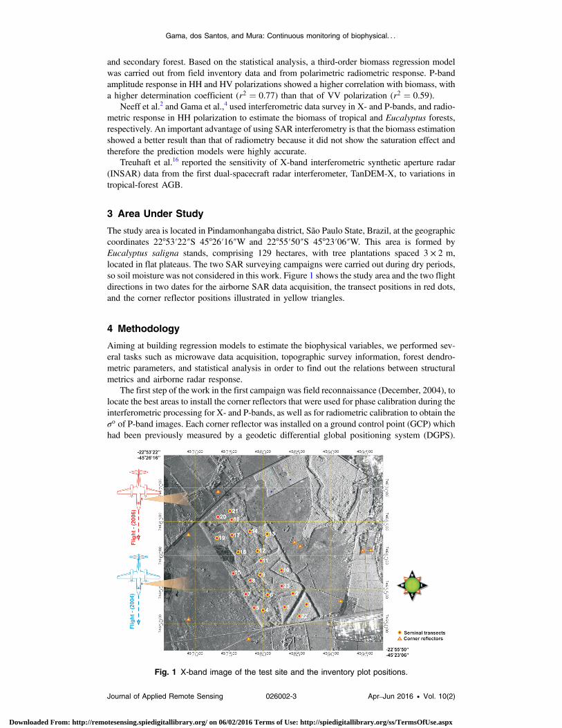
The study area is located in Pindamonhangaba district, São Paulo State, Brazil, at the geographiccoordinates 22°53′22″S 45°26′16″W and 22°55′50″S 45°23′06″W. This area is formed byEucalyptus saligna stands, comprising 129 hectares, with tree plantations spaced 3 × 2 m,located in flat plateaus. The two SAR surveying campaigns were carried out during dry periods,so soil moisture was not considered in this work. Figure 1 shows the study area and the two flightdirections in two dates for the airborne SAR data acquisition, the transect positions in red dots,and the corner reflector positions illustrated in yellow triangles.

4 Methodology

Aiming at building regression models to estimate the biophysical variables, we performed sev-eral tasks such as microwave data acquisition, topographic survey information, forest dendro-metric parameters, and statistical analysis in order to find out the relations between structuralmetrics and airborne radar response.

The first step of the work in the first campaign was field reconnaissance (December, 2004), tolocate the best areas to install the corner reflectors that were used for phase calibration during theinterferometric processing for X- and P-bands, as well as for radiometric calibration to obtain theσo of P-band images. Each corner reflector was installed on a ground control point (GCP) whichhad been previously measured by a geodetic differential global positioning system (DGPS).

Fig. 1 X-band image of the test site and the inventory plot positions.




These DGPS trackings were carried out by the static relative method, using an official first ordersatellite base, which allowed obtaining a 5.0-cm plani-altimetric coordinate precision.

In addition to setting up the GCPs, it was necessary to use a high-precision geographic refer-ence point at the same airport used by the airplane. This point was tracked by a geodetic GPSduring the flight survey to allow the generation of the attitude vector radar by the airborne inertialmeasurement unit (IMU) processing.

A topographic survey was carried out using a Topcon total station, model GTS-701, with 3″of accuracy and 10-m spacing, covering all transects and some pasture areas in order to locate theplots in the images and to evaluate the digital elevation models (DEMs). The measured startingpoint was the same as the one used to support the corner reflector and to perform the final meas-urement, which allowed topographic adjustments describing a closed polygon, and whichobtained a 5-cm precision in the final adjustments.

For the acquisition of radar data, the OrbiSAR-1 radar from BRADAR Company (Orbisat)was used, which allowed us to generate DEM by SAR interferometry at two different frequen-cies, X (λ ¼ 3 cm) and P (λ ¼ 72 cm) bands.

OrbiSAR-1 operates in four polarizations in P-band, so it was possible to obtain the DEMand the Coh in four different polarizations (CohPHH, CohPHV, CohPVH, and CohPVV). Bothsurveying campaigns (2004 and 2006) obtained final mappings in scale 1: 25,000 forP-band and 1: 10,000 for X-band, whose end pixel size was 2.0 m for P-band and 1.0 mfor X-band, with the same values for the respective altimetry. The X-band interferometrywas performed in one-pass acquisition with 2.77 m of baseline, generating coherence image,DEM and complex image in HH polarization; while for P-band interferometry, 50 m of baselinewas used in two-passes. The difference of the DEM by interferometry in X- and P-bands wasconsidered as Hint, and used as a variable during the building of the regression models.

The biophysical models were built by statistics regression from the SAR surveying and forestinventory in 2004 (Gama et al.4), in which the parameters DBH, height, and volume could beestimated from interferometric radar data (σo, DEM, and Coh).

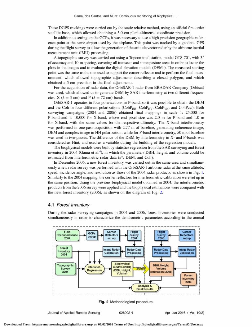
In December 2006, a new forest inventory was carried out in the same area and simultane-ously a new radar survey was performed with the OrbiSAR-1 airborne radar at the same altitude,speed, incidence angle, and resolution as those of the 2004 radar products, as shown in Fig. 1.Similarly to the 2004 mapping, the corner reflectors for interferometric calibration were set up inthe same position. Using the previous biophysical model obtained in 2004, the interferometricproducts from the 2006 survey were applied and the biophysical estimations were compared withthe new forest inventory (2006), as shown on the diagram of Fig. 2.

4.1 Forest Inventory

During the radar surveying campaigns in 2004 and 2006, forest inventories were conductedsimultaneously in order to characterize the dendrometric parameters according to the annual

Fig. 2 Methodological procedure.




inventory tracking. The inventory was carried out in 23 independent plots of ∼400 m2 each, inwhich the DBH and total tree height were measured. Allometric equations based on height,diameter, and form factor were used to calculate tree volume. Equation (1) shows the allometricequation for volume estimation and the corresponding form factors used for each range of DBHmeasured in the inventory.

EQ-TARGET;temp:intralink-;e001;116;675

Volume ¼�

DBH2�π4

�� TotalHeight � FF DBH FF

FF ¼ Formfactor 4.0 − 12.0 0.46

12.0 − 20.0 0.44

20.0 − 28.0 0.42

(1)

4.2 Radar Data Processing

The Orbisat Company provided the software to process the SAR raw data in order to obtain theimages and the interferometry SAR products. The images were processed with four looks tominimize the speckle noise, and then converted to ground range and orthorectified using thecorresponding DEM generated during the interferometric processing. Rombach et al.17 describedthe details of the data transcription, IMU processing, and SAR data processing to obtain SARproducts.

The radiometry of P-band complex images was calibrated by the Radar Tools software (RAT0.16.2 version), which provided cross talk processing, channel imbalance processing, and polari-metric calibration using a corner reflector response based on Quegan18 approach.

To calibrate the SAR data, nine corner reflectors of the same size, 1.5-m side length, weredistributed between near and far ranges in the area and used for the polarimetric and interfero-metric calibrations. To acquire σo images, the corner reflector peak response was used (Zinket al.,19 Santos et al.1) obtaining a correction factor to transform the P band amplitude imagesby interactive data language (IDL) routines.

The azimuth and elevation angles of the corner reflectors were calculated based on the flightplan and on the high-accuracy (5 cm) GCP geographic coordinates, the incidence angle of whichdid not present large variations.

The SAR data was generated using the Orbisat Company software, which allowed obtainingorthorectified SAR images using the corresponding digital elevation models. Details about theOrbisat software for data transcription, IMU and SAR data processing to obtain DEM, orthoi-mages, and coherences are described by Rombach et al.17

The radar cross section of each corner reflector was measured and a linearity behavior wasverified. The signal to noise ratio, the antenna pattern, radar losses, and radar illumination geom-etry were also considered.

The corner reflector responses were also used for the phase calibration during the interfero-metric calibration in order to obtain the DEM in X and P bands. For polarimetric calibration, theQuegan18 methodology was used for the cross-talk processing and channel imbalance by thesecorner reflector responses.

4.3 Statistical Modeling

To build the regression models, the variable selection criteria suggested by Neter et al.20 wereused, such as coefficient of determination (r2), adjusted coefficient of determination (r2a), Cpcriterion (Neter et al.20), and Stepwise criterion, using Statistica 6.0 version software.

The coefficient r2a employs a weighting for the extent of regression adjustment, making itmore relevant than the coefficient r2. Cp criterion involves the concept of total mean square errorfor each subset of the adjusted regression models, which considers the total error in each valueset. Cp criterion can identify subsets of dependent variables in which the total mean squared erroris small, i.e., when the Cp value is equal or close to the number of p parameters, this model willbe less biased. The forward stepwise procedure gradually adds a new variable to the model, andextracts that part whose contribution was not considered significant by an F-test. Equation (2)shows the Cp criterion estimation




EQ-TARGET;temp:intralink-;e002;116;735Cp ¼�

SSEp

MSEðX1; : : : : : : Xp−1Þ�− ðn − 2pÞ; (2)

where SSEp is the error sum of squares for the fitted subset regression model with p parameters(with p − 1 × variables), and mean squared error (MSE).

Levene’s test was used for the heteroscedasticity evaluation (constancy of residue variance),which performs the comparison t-test of two subgroups of data set samples to determine whetherthe average absolute deviation of a subgroup differs from the other. Cook’s distance method wasused to assess the existence of outliers in the data set (Neter et al.20), which considers the in-fluence of a specific observation in all other adjusted values. A sample can be considered anoutlier when its percentile of F distribution exceeds 20%.

For model validation of small data sets, prediction sum of squares (PRESS) criterion is usedas a way to evaluate the prediction model. The test works by eliminating the i’th case of the dataset, estimating the regression function with the remaining observations, then using the adjustedregression equation to obtain the predicted value. The quadratic sum of all these n predictionerrors defines the PRESS value. According Neter et al.,20 the closeness between PRESS anderror sum of squares (SSE) values, indicates that the MSE value can be a reasonable indicatorof the model predictive ability.

5 Results and Discussion

5.1 Forest Inventory

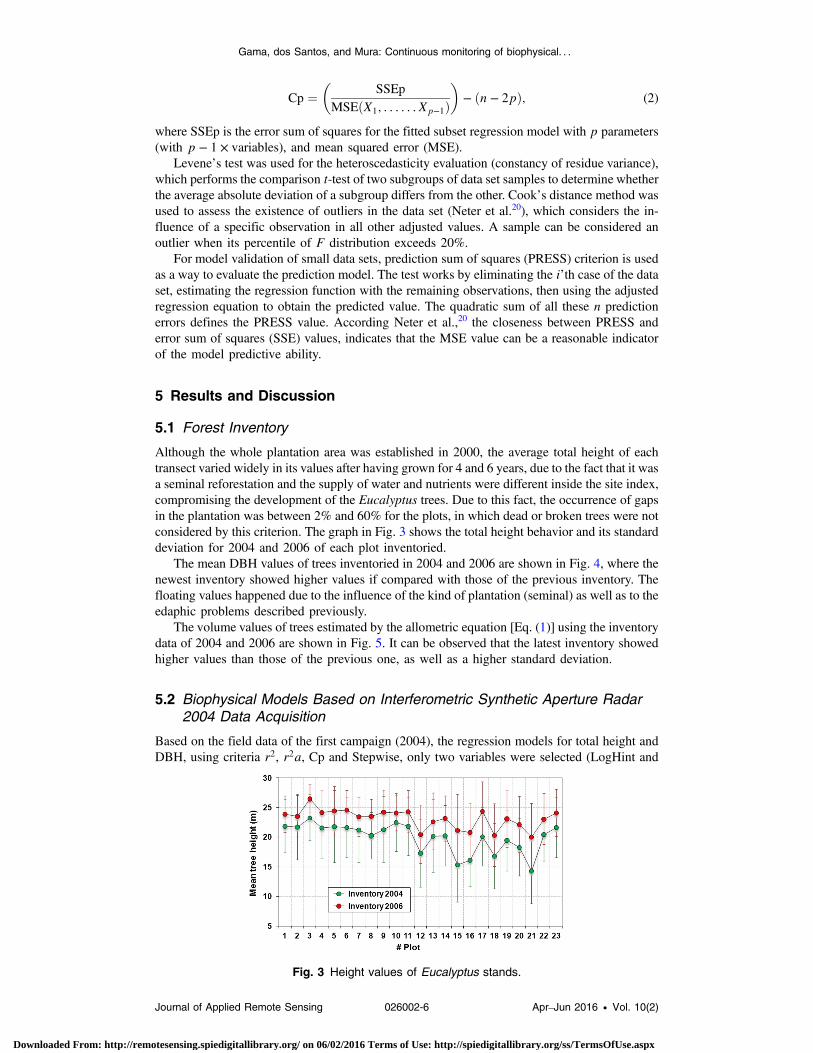
Although the whole plantation area was established in 2000, the average total height of eachtransect varied widely in its values after having grown for 4 and 6 years, due to the fact that it wasa seminal reforestation and the supply of water and nutrients were different inside the site index,compromising the development of the Eucalyptus trees. Due to this fact, the occurrence of gapsin the plantation was between 2% and 60% for the plots, in which dead or broken trees were notconsidered by this criterion. The graph in Fig. 3 shows the total height behavior and its standarddeviation for 2004 and 2006 of each plot inventoried.

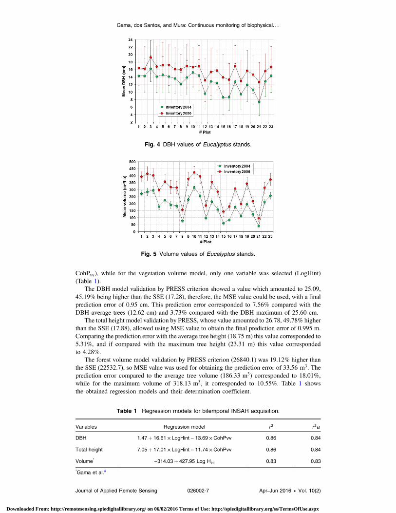
The mean DBH values of trees inventoried in 2004 and 2006 are shown in Fig. 4, where thenewest inventory showed higher values if compared with those of the previous inventory. Thefloating values happened due to the influence of the kind of plantation (seminal) as well as to theedaphic problems described previously.

The volume values of trees estimated by the allometric equation [Eq. (1)] using the inventorydata of 2004 and 2006 are shown in Fig. 5. It can be observed that the latest inventory showedhigher values than those of the previous one, as well as a higher standard deviation.

5.2 Biophysical Models Based on Interferometric Synthetic Aperture Radar2004 Data Acquisition

Based on the field data of the first campaign (2004), the regression models for total height andDBH, using criteria r2, r2a, Cp and Stepwise, only two variables were selected (LogHint and

Fig. 3 Height values of Eucalyptus stands.




CohPvv), while for the vegetation volume model, only one variable was selected (LogHint)(Table 1).

The DBH model validation by PRESS criterion showed a value which amounted to 25.09,45.19% being higher than the SSE (17.28), therefore, the MSE value could be used, with a finalprediction error of 0.95 cm. This prediction error corresponded to 7.56% compared with theDBH average trees (12.62 cm) and 3.73% compared with the DBH maximum of 25.60 cm.

The total height model validation by PRESS, whose value amounted to 26.78, 49.78% higherthan the SSE (17.88), allowed using MSE value to obtain the final prediction error of 0.995 m.Comparing the prediction error with the average tree height (18.75 m) this value corresponded to5.31%, and if compared with the maximum tree height (23.31 m) this value correspondedto 4.28%.

The forest volume model validation by PRESS criterion (26840.1) was 19.12% higher thanthe SSE (22532.7), so MSE value was used for obtaining the prediction error of 33.56 m3. Theprediction error compared to the average tree volume (186.33 m3) corresponded to 18.01%,while for the maximum volume of 318.13 m3, it corresponded to 10.55%. Table 1 showsthe obtained regression models and their determination coefficient.

Fig. 5 Volume values of Eucalyptus stands.

Table 1 Regression models for bitemporal INSAR acquisition.

Variables Regression model r 2 r 2a

DBH 1.47þ 16.61 × LogHint − 13.69 × CohPvv 0.86 0.84

Total height 7.05þ 17.01 × LogHint − 11.74 × CohPvv 0.86 0.84

Volume* −314.03þ 427.95 Log Hint 0.83 0.83

*Gama et al.4

Fig. 4 DBH values of Eucalyptus stands.




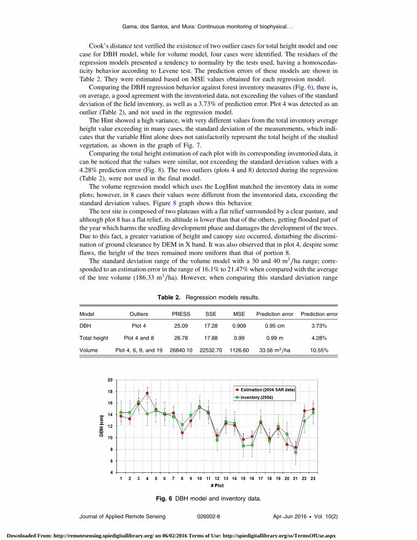
Cook’s distance test verified the existence of two outlier cases for total height model and onecase for DBH model, while for volume model, four cases were identified. The residues of theregression models presented a tendency to normality by the tests used, having a homoscedas-ticity behavior according to Levene test. The prediction errors of these models are shown inTable 2. They were estimated based on MSE values obtained for each regression model.

Comparing the DBH regression behavior against forest inventory measures (Fig. 6), there is,on average, a good agreement with the inventoried data, not exceeding the values of the standarddeviation of the field inventory, as well as a 3.73% of prediction error. Plot 4 was detected as anoutlier (Table 2), and not used in the regression model.

The Hint showed a high variance, with very different values from the total inventory averageheight value exceeding in many cases, the standard deviation of the measurements, which indi-cates that the variable Hint alone does not satisfactorily represent the total height of the studiedvegetation, as shown in the graph of Fig. 7.

Comparing the total height estimation of each plot with its corresponding inventoried data, itcan be noticed that the values were similar, not exceeding the standard deviation values with a4.28% prediction error (Fig. 8). The two outliers (plots 4 and 8) detected during the regression(Table 2), were not used in the final model.

The volume regression model which uses the LogHint matched the inventory data in someplots; however, in 8 cases their values were different from the inventoried data, exceeding thestandard deviation values. Figure 8 graph shows this behavior.

The test site is composed of two plateaus with a flat relief surrounded by a clear pasture, andalthough plot 8 has a flat relief, its altitude is lower than that of the others, getting flooded part ofthe year which harms the seedling development phase and damages the development of the trees.Due to this fact, a greater variation of height and canopy size occurred, disturbing the discrimi-nation of ground clearance by DEM in X band. It was also observed that in plot 4, despite someflaws, the height of the trees remained more uniform than that of portion 8.

The standard deviation range of the volume model with a 30 and 40 m3∕ha range; corre-sponded to an estimation error in the range of 16.1% to 21.47% when compared with the averageof the tree volume (186.33 m3∕ha). However, when comparing this standard deviation range

Table 2. Regression models results.

Model Outliers PRESS SSE MSE Prediction error Prediction error

DBH Plot 4 25.09 17.28 0.909 0.95 cm 3.73%

Total height Plot 4 and 8 26.78 17.88 0.99 0.99 m 4.28%

Volume Plot 4, 6, 9, and 19 26840.10 22532.70 1126.60 33.56 m3∕ha 10.55%

Fig. 6 DBH model and inventory data.




with the volume of the biggest trees (318.13 m3∕ha), the error corresponded to a range of 9.43%to 12.57%.

5.3 Models Performance with Interferometric Synthetic Aperture Radar 2006Data

Using the regression model generated in 2004, the DBH estimation for 2006 showed agreementwith the inventoried data in relation to the mean values for a great number of cases except 4,which showed an overestimation that surpassed the inventory standard deviation. The graph inFig. 9 shows the obtained results.

Similar to the DBH estimation, the tree height estimation showed four cases with an over-estimation that surpassed the inventory standard deviation. The remaining 19 cases were similarto the inventory or were inside the inventory standard deviation values. The graph in Fig. 10shows the obtained results.

Analyzing the behavior of the Eucalyptus mean height of each plot with its correspondingDBH, a linear relationship between these biophysical variables was observed without significantoutliers, whose linear regression showed an r2 of 0.987 for the 2004 inventory and 0.997 for the2006 inventory. A progression of height and DBH responses can also be observed, indicatingthat the vegetative growth at the study area elapsed 2 years. The estimation values of the meantree heights and the mean DBH, also showed a linear behavior (Fig. 11), like the inventory data,with a continuity of the tendency of the regressions; the 2004 r2 estimation was 0.991 while itwas 0.995 for 2006.

Fig. 8 Volume estimated and inventory data.

Fig. 7 Total height estimated and inventory data.




Fig. 10 Mean values of tree height estimation and the inventory data.

Fig. 9 Mean values of DBH estimation and inventory data.

Fig. 11 Mean values of tree height and DBH of Eucalyptus stands.




On the other hand, when comparing the inventoried and estimated volume for these twodates, the result was linear with little dispersion, i.e., 0.948 of r2, while 0.968 for inventoriedvolume.

Analyzing the tree volume model response, it can be noticed that inventoried and estimatedvalues (Fig. 12) had a linear behavior with a high r2 value, but an error estimation of 10.55%,acceptable for forest surveying, which considers 10% as a typical inventory error.

Based on the obtained regression models, a hypsometric image for the total height, DBH andvolume was generated using the CohPvv and LogHint images, achieving a final image whosepixel values corresponded to numerical values of the regression. For the visualization of a com-bination of results of the regression model image data and the radiometric response in the X bandwas performed using the IHS technique (I = intensity, H = hue, S = saturation), which, for allmodels, was defined: 50% for saturation (S) and the X-band amplitude image as the intensity (I).

The result of the IHS image referring to total height estimation using the SAR from 2004 isshown in Fig. 13(a), along with a range of colors that corresponds to the total height estimated.Color gradients with predominance on the heights of ∼14 and ∼20 m are shown. The regions ofimage in blue color correspond to zero point, resulting from settlement failures.

The hypsometric image of Fig. 13(b) corresponds to the total height estimated using theregression model generated in 2004 with the 2006 SAR data. Analyzing the linear regressionof the 2006 inventory data and the total height model results, MSE value of 1.39 m was obtained,

Fig. 12 Tree volume inventoried and estimated.

Fig. 13 IHS (I = X-band, H = total height estimation, S = 50%): (a) 2004 estimation and (b) 2006estimation.




which represented 1.18 m, or 4.84% of prediction error, when compared with higher values oftree heights.

The hypsometric image of Fig. 14(a) was generated using the DBH regression model, and thecorresponding SAR data from 2004, obtaining an image whose pixel values correspond tonumerical values of the regression, with a spatial resolution of 1.9 m. It can be noticedfrom Fig. 14(a) that part of the test site has predominance in the DHP values ∼10 to∼15 cm. The regions of the image in blue correspond to DHP null values, resulting fromthe failure of the stand.

The hypsometric image of Fig. 14(b) corresponds to the DBH estimated for 2006, using theregression model generated in 2004, and the SAR data from 2006. Using linear regression withthe 2006 inventory data and the DBH model results, MSE of 1.63 cm was obtained, whichrepresented 1.28 cm, or 6.62% of prediction error, when compared with higher values of DBH.

Using the regression model generated in 2004, it was possible to yield an IHS image of theforestry volume, whose results were shown in the hypsometric image of Fig. 15(a). For theobtained color image gradients, it can be noticed that the volume values ranged between 0and ∼400 m3∕ha. The stand failures are represented in blue color, corresponding to low volumevalues.

The hypsometric image of Fig. 15(b) is an IHS image that corresponded to the volume esti-mated for 2006, using the regression model generated in 2004, and the SAR data from 2006. The

Fig. 14 IHS (I = X-band, H = DBH estimation, S = 50%): (a) 2004 estimation and (b) 2006estimation.

Fig. 15 IHS (I = X-band, H = volume estimation, S = 50%): (a) 2004 estimation and (b) 2006estimation.




linear regression of the 2006 inventory data and the volume model results, presented a MSEvalue of 2448.01 m3∕ha, which represented 49.48 m3∕ha, or 11.96% of prediction error if com-pared with higher values of tree volume.

Although the planting occurred in the same period, the average total height of each transectpresented a wide range of values after 4 and 6 years of development, since it is a seminal refor-estation and the provision of water and nutrients varies in the area, which hinders the Eucalyptusdevelopment. Additionally the occurrence of gaps between 2% and 60% inside the plots wasverified. So, this characteristic induced intermediate height measurements rather than groundheight, disturbing the Hint measurement (X-band DEM minus P-band DEM) that wouldinfer the tree heights, as illustrated in Fig. 16(a) and observed in Fig. 16(b).

As in the regions with trees the Coh in the P-band is high, and in clear areas the P-bandcoherence is low, the presence of this variable in the total height and DBH models compensatedthe gap effects, improving the model performance as shown in graphs of Figs. 6 and 7.

When these models were used with the second acquisition data from airborne radar (2006),the estimation errors were a little higher if compared with those of 2004 used as a reference basis.One of the reasons for the slight decrease in performance can be explained by significantdifferences between Eucalyptus stands of different ages, which result in variations of the mor-phometric parameters canopy. With the growth of the individual trees tend to have a faster devel-opment of the trunk, compared to the development of the crown; i.e., the coverage ratio, salienceindex and living space index decrease with the growth of trees and the increasing size inside theforest stand. Thus, due to these variations of the percentage of the gaps, consequently theCohPvv and/or Hint contribution did not fit in some cases.

Nevertheless, the errors for DBH and total height models would still be suitable for forestsurveying, which considers 10% as a typical inventory error. For volume prediction the error was1.96% beyond this limit.

6 Conclusions

The use of the biophysical models created in the first imaging campaign, along with field andradar data from the second campaign carried out two years later, were consistent and the resultsare very promising for updating annual inventories required in Eucalyptus planting managementaiming at cellulose production.

For the vegetation volume model, only the X-band interferometric surveying would be nec-essary for the annual volume estimations, because the model only uses the logHint variable.Therefore, this approach decreases surveying costs, once the generation and processing ofnew data in P-band would not be necessary, since P-band interferometry demands two passesand X-band interferometry demands only one pass. Another possibility to be evaluated would bethe use of X-band interferometry by the satellites TerraSAR/TanDEM or Cosmo SKYMED, in

Fig. 16 (a) Gaps and ground truth (red and blue lines: X-band DEM, black line: P-band DEM) and(b) Hint (X-band DEM minus P-band DEM) of the plot showing the gaps effect.




order to generate the DEM, but it would be necessary to have a P-band or L-band DEM inadvance.

We recommend carrying out further research for steep relief, in order to verify its effect onprediction models due to the fact that the area under study in this article is practically flat. Asrelief variations modify local incidence angle, they can change the target interaction, and inextreme cases cause foreshortening and shadowing effects.

Acknowledgments

The authors acknowledge the help of the 5th Surveying Army Division (Brazilian Army),Nobrecel Celulose and Papel S.A., Diâmetro Biometria & Inventário Florestal, BRADARAerolevantamento S.A. (ORBISAT) for their support in this research, and CNPq for a grantreceived by the second author.

References

1. J. R. Santos et al., “Airborne P-band SAR applied to the above ground biomass studies in theBrazilian tropical rainforest,” Remote Sens. Environ. 87, 482–493 (2003).

2. T. Neeff et al., “Tropical forest measurement by interferometric height modeling and P-bandbackscatter,” Forest Sci. 51(6), 585–594 (2005).

3. J. O. Sexton et al., “A comparison of LIDAR, radar, and field measurements of canopyheight in pine and hardwood forests of southeastern North America,” For. Ecol.Manage. 257, 1136–1147 (2009).

4. F. F. Gama, J. R. dos Santos, and J. C. Mura, “Eucalyptus biomass and volume estimationusing interferometric and polarimetric SAR data,” Remote Sens. 2, 939–956 (2010).

5. P. C. Bispo et al., “Integration of polarimetric PALSAR attributes and local geomorpho-metric variables derived from SRTM for forest biomass modeling in central amazonia,”Can. J. Remote Sen.: J. Can. de Teledetection 40(1), 26–42 (2014).

6. N. P. Joshi et al., “L-band SAR backscatter related to forest cover, height and abovegroundbiomass at multiple spatial scales across Denmark,” Remote Sens. 7, 4442-4472 (2015).

7. M. Santoro, L. E. B. Eriksson, and J. E. S. Fransson, “Reviewing ALOS PALSAR back-scatter observations for stem volume retrieval in swedish forest,” Remote Sens. 7, 4290–4317 (2015).

8. Y. Rauste et al., “Radar-based forest biomass estimation,” Int. J. Remote Sens. 15, 2797–2808 (1994).

9. K.O. Pope, J.M. Rey-Benayas, and J.F. Paris, “Radar remote sensing of forest and wetlandecosystems in the central American tropics,” Remote Sens. Environ. 48, 205–219 (1994).

10. M. Borgeaud and U. Wegmueller, “On the use of ERS SAR interferometry for retrieval ofgeo- and biophysical information,” in Proc. of the ‘FRINGE 96’ Workshop on ERS SARInterferometry, Zurich, Switzerland (1996).

11. E. S. Kasischke, J. M. Melack, and M. C. Dobson, “The use of imaging radars for ecologicalapplications—a review,” Remote Sens. Environ. 59, 141–156 (1997).

12. S.R. Cloude and E. Pottier, “An entropy based classification scheme for land applications ofpolarimetric SAR,” IEEE Trans. Geosci. Remote Sens. 35, 68–78 (1997).

13. T. Le Toan and N. Floury, “On the retrieval of forest biomass from SAR data,” in Proc. of the2nd Int. Symp. on Retrieval of Bio- and Geo-physical Parameters from SAR data for LandApplications, ESTEC, Noordwijk, The Netherlands (1998).

14. D. G. Leckie and K. J. Ranson, “Forestry applications using imaging radar,” in Principles &Applications of Imaging Radar: Manual of Remote Sensing, R. A. Ryerson, Ed., 3th ed.,Vol. 2, pp. 435–509, John Wiley & Sons, Inc., New York, NY (1998).

15. J. C. Mura et al., “Identification of the tropical forest in Brazilian Amazon based on theMNT difference from P and X bands interferometric data,” In Proc. of IEEE Geoscience andRemote Sensing Symp., Sydney, Australia (2001).

16. R. Treuhaft et al., “Tropical-forest biomass estimation at X-Band from the spaceborneTanDEM-X interferometer,” IEEE Geosci. Remote Sens. Lett. 12(2), 239–243 (2015).




http://dx.doi.org/10.1016/j.rse.2002.12.001

http://dx.doi.org/10.1016/j.foreco.2008.11.022

http://dx.doi.org/10.1016/j.foreco.2008.11.022

http://dx.doi.org/10.3390/rs2040939

http://dx.doi.org/10.1080/07038992.2014.913477

http://dx.doi.org/10.3390/rs70404442

http://dx.doi.org/10.3390/rs70404290

http://dx.doi.org/10.1080/01431169408954285

http://dx.doi.org/10.1016/0034-4257(94)90142-2

http://dx.doi.org/10.1016/S0034-4257(96)00148-4

http://dx.doi.org/10.1109/36.551935

http://dx.doi.org/10.1109/LGRS.2014.2334140

17. M. Rombach et al., “Newest Technology of mapping by airborne interferometric syntheticaperture radar system,” IEEE Trans. Geosci. Remote Sens. 7, 4450–4452 (2003).

18. S. A. Quegan, “Unified algorithm for phase and cross-talk calibration of polarimetricdata—Theory and observations,” IEEE Trans. Geosci. Remote Sens. 32, 89–99 (1994).

19. M. Zink and R Bamler, “X-SAR radiometric calibration and data quality,” IEEE Trans.Geosci. Remote Sens. 33, 840–847 (1995).

20. J. Neter et al., “Applied Linear Statistical Models,” 4th ed., McGraw-Hill, Boston, MA(1996).

Fábio Furlan Gama graduated in electronic engineering from the Vale do Paraiba University,Sao Jose dos Campos, Brazil, in 1986 and received his MS and PhD degrees in remote sensingfrom the National Institute for Space Research (INPE), Sao Jose Campos, Brazil, in 1996 and2007, respectively. He currently works at INPE, as a senior researcher in the Image ProcessingDepartment in development and applications of polarimetry and interferometry SAR. Hisresearch interests include SAR interferometry, differential SAR interferometry, SAR polarim-etry, and applications of SAR surveying for land use/cover.

João Roberto dos Santos received his BSc degree in forestry engineering from the FederalRural University of Rio de Janeiro, Brazil—UFRRJ in 1974. He received his MSc degree inremote sensing from INPE in 1979 and his PhD in forest science from the FederalUniversity of Paraná—UFPR, 1988. He is a senior researcher in the Remote SensingDivision of INPE, whose current activities are optical and SAR applications for the inventoryand monitoring of forest typologies

José Claudio Mura graduated in electrical engineering from the School of Engineering of SãoCarlos USP, 1978, received his master’s degree in electronics and computer engineering from theTechnological Institute of Aeronautics, 1985, and his PhD in applied computing from the INPE,2000. He is a senior researcher at INPE. He has experience in computer science, with emphasison methodology and technical computing, acting on the following topics: SAR interferometry,SAR polarimetry, and SAR calibration. Currently, he is working in the field of differential inter-ferometric SAR images to estimate surface deformation using orbital radar sensor data




http://dx.doi.org/10.1109/IGARSS.2003.1295543

http://dx.doi.org/10.1109/36.285192

http://dx.doi.org/10.1109/36.406670

http://dx.doi.org/10.1109/36.406670

continuous monitoring of biophysical eucalyptussp...

Documents