continuous wave radars–monostatic, …€¦ · · 2005-07-29abstract radar technology was...

CONTINUOUS WAVE

RADARS–MONOSTATIC,

MULTISTATIC AND NETWORK

Krzysztof KulpaWarsaw University of Technology

00-665 Warsaw, Poland

Abstract Radar technology was designed to increase public safety on sea and inthe air. Today radars are used in many fields of application, such as air-defense, air-traffic-control, zone protection (in military bases, airports,industry), people search and others. Classic pulse radars are often be-ing replaced by continuous wave radars. Unique features of continuouswave radars, such as the lack of ambiguity, very low transmitted powerand good electromagnetic compatibility with other radio-devices, en-hance this trend. This chapter presents the theoretical background ofcontinuous wave radar signal processing (for FMCW and noise radars),highlights the most important features of this type of radar and showstheir abilities in the field of security.

Keywords: continuous wave radar; linear frequency modulation; noise radar; noise;modulation; correlation function; ambiguity function; synthetic aper-ture; radar; target identification.

1. Introduction

Today security technology migrates from strictly military areas tomany different civil applications. On one hand this migration is causedby the high risk of terrorist threats, on the other one observes the grow-ing interest of society in protecting personal life regardless of the costs ofrescue operations. Many sophisticated technologies are in everyday useto protect people in airports, shopping centers, schools and other pub-lic places. Strong efforts have been made to locate people in buildingsand ruins during rescue and peacekeeping missions. One of the mostimportant security problems is to remotely detect and localize objectsof interest (often referred to as targets) and to distinguish between thetarget and its environment. Another issue is to extract as much use-ful information about the object as possible and to classify it properly.

2

The process of detection can be performed by using different sensingtechnologies and different sensors.

One very common and mature technology is based on optical sens-ing, which is used in many military and civilian areas such us “citysurveillance”. Optical cameras convert the electromagnetic object sig-nature into an image of the target, which can be further processed andstored by the computer. However, this technology faces many limita-tions. Working in the visual light region it is necessary to illuminate thetarget either by natural light sources (sunlight, moonlight) or artificialilluminators (street lights, reflectors etc). Some interesting results canbe achieved by using other parts of the electromagnetic spectrum. Deepinfrared cameras can provide images in a completely dark environment,but they require a temperature difference between the target and its sur-roundings. Their detection range is usually very limited and detectionis impossible or very difficult in bad weather conditions or behind fire,smoke and obstacles.

For a long time radio frequency emission has been used for targetdetection and tracking. Classical radar senses the object by emittingshort, powerful electromagnetic pulses towards the target and listeningto the return echo. The distance to the target is calculated from thedelay of the echo signal. It is also possible to estimate the direction ofthe target, its velocity and, using more sophisticated synthetic apertureradar (SAR)/Inverse SAR (ISAR) technology, the target size and shape.Having all this information, it is possible to recognize and track differentobjects. This radar technology is independent of weather and day/nightconditions, and may be used to detect targets hidden by obstacles, wallsor even buried in the ground. However, pulse radar technology has manydisadvantages. To achieve large detection range, high power transmittersare required. Due to the pulse nature of such radars, there are manyambiguity problems. Pulse radars can be easily detected by very simpleelectronic support measurement devices, which is a big disadvantage forcovert security missions.

A present trend in radar technology is to decrease the emitting peakpower. Instead of emitting a train of high power pulses, it is possible toemit a low-power continuous signal with appropriate modulation. Ad-vanced signal processing of the received signal allows radars to detecttarget echoes far below the surrounding noise level and to extract all re-quired target parameters. It is also possible to produce high-resolutiontarget pictures. In some applications it is even not necessary to emit anilluminating signal, but to exploit existing radio, TV or other emissions.

A single sensor usually has limited range and accuracy — especially inthe cross-range direction. The use of bistatic ideas, where the transmit-

Continuous wave radars–monostatic, multistatic and network 3

ter and receiver are separated in space, leads to a new technology withincreased sensitivity and accuracy in selected regions. Increasing thenumber of sensors (multistatics) yields much bigger surveillance volume,much higher probability of detection and proper target classification.This technology is also much more robust to target shadowing, multi-path signal fading and jamming. To fully use the information producedby the set of sensors, it is necessary to exchange information betweensensors and generalize this information. This leads to the net-centricsensor concept.

Radar devices were primary designed to increase public safety and noware used in many security applications. The most obvious applicationfields are air traffic control (ATC) and air defense. Battlefield short ormiddle-range radar can now detect, track and identify slow moving tar-gets such as tanks, cars, pedestrians and animals. Using micro-Doppleranalysis, it is possible to identify vehicles, and using vibration analy-sis, to even distinguish between two cars of the some brand. Heartbeatanalysis is used for people identification and, together with breathinganalysis, can even provide information on the emotional state of eachperson. Walk analysis based on Doppler processing and walk modelingare being used for person tracking even in crowded areas. Ground-penetrating and wall-penetrating radars are used to search for people inrescue operations, when it is necessary to search big areas of ruins oravalanches. One of the most important security issues is to distinguishbetween people and animals, in order to save human life first. A bigarea of security is connected with trespass control as well. It is very im-portant for border protection, airport and military base protection andelsewhere.

2. Radar fundamentals

The concept of radar was discovered in the beginning of the 20th cen-tury. The “father” of radar was Christian Huelsmeyer, who applied for apatent for his “telemobiloscope” on 30 April 1904. He was motivated inhis work by a ship accident and his intention was to construct a deviceto boost the level of safety. His device worked reasonably well, detectingships at ranges up to 3 km in all weather conditions, but he had no suc-cess in selling telemobiloscopes and that early radar concept faded frommemory. The reinvention of radar was done almost simultaneously inmany countries in the 1920’s and 30’s. In Great Britain, work on radartechnology was carried out by the physicist Sir Edward Victor Appleton,who used radio echoes to determine the height of the ionosphere in 1924.The first demonstration of aircraft detection was done by Watson-Watt

4

and Wilkins, who had used radio-wave transmissions from the powerfulBBC short-wave station at Daventry and measured the power reflectedfrom a Heyford bomber. Detection was achieved at at distance of up to 8miles. As a matter of fact, this was the first demonstration of a bistatic,continuous wave passive radar. The first British radar patent was issuedin April 1935. In the United States radar research was carried out in theearly 1920’s by Dr. A. Hoyt Taylor at the Naval Research Laboratory inWashington, D.C. Radar research was also carried out in France and in1934 the French liner “Normandie” was equipped with a “radio obstacledetector”. Work on radar technology was also carried out in many othercountries, but usually such research was classified.

Early radars were non-coherent pulse radars. To obtain long rangedetecting capability, the radar emits short pulses with very high peakpower — up to several megawatts. The detection range limitation usu-ally comes from the inadequacy of the maximum peak power. Availablemicrowave valves and waveguides limit this parameter. To decrease therequired peak power pulse compression techniques have been worked out.The first radars were used for air defense to indicate moving targets. Allground echoes were unwanted, and to distinguish between ground clutterand moving targets Doppler processing was introduced. Long distancepulse radar suffered from range or Doppler ambiguity. It is not pos-sible to measure instantaneously both range to the target and targetradial velocity, without the ambiguity given by the sampling theorem.The pulse radar concept was relatively simple and pulse radars couldbe designed using only analogue components. The problem with signalstorage, required for Doppler processing, was solved by using acousticdelay lines (e.g. mercury tubes) or memo-scope bulbs.

Rapid progress in digital signal processing (DSP) hardware and algo-rithms enabled designers to exploit more complicated ideas. One suchidea was to use continuous wave (CW) instead of high power short pulses.The idea was not new — the first Daventry experiment was based onCW radio emission, but practical implementation of CW radars was im-possible without digital technology. The first practical continuous waveradars were constructed as Doppler-only radars. The well known policeradar belongs to that group. Further development in CW radars leadto linear frequency modulated CW radars (LMCW), in which both tar-get range and range velocity can be measured. But again, due to theperiodicity in modulation, the ambiguity problem was still there.

CW radars have a very big advantage — very low peak power. Asthe transmitted power can be below 1 W (many of them work with 1mW power), they belong to the low probability of intercept (LPI) classof radars, which can detect targets while they remain undetected.


The search for ambiguity-free waveforms has lead to the conceptof random-waveform radars, often referred to as noise or pseudo-noiseradars. In this kind of radar, the target is illuminated by continuousnoise-like radiation. The reflected power is collected by the radar re-ceive antenna, and detection is based on match filtering of the receivedsignals. The single filter is matched to the particular value of range andrange velocity. Because the target’s distance and speed are unknown, itis necessary to apply a set of filters matched to all possible range-velocitypairs. The computational power required by the noise radars is muchhigher than for other radar types, so to date noise radars have not beenused very much. There are also other drawbacks of noise radars. Due tothe fact that the noise radar has to emit and receive signals simultane-ously, good separation between transmitting and receiving antennas isrequired. Furthermore, this radar simultaneously receives strong echoesoriginating from close targets, buildings and ground, and weak echoesfrom distant targets. Thus, a large receiver dynamic range is needed.

The noise-radar concept may be used for moving target detectionand also for many other applications. There are several works showingpossible implementation of noise technology for imaging radar workingin SAR or ISAR mode, passive detection and identification of targetsand space radiometric applications. Noise radars will also be used in thefuture in other fields, including air traffic control, pollution control, andespecially security applications.

2.1 Radar range equation

Classical pulse radar emits high power (PT ) short electromagneticpulses using a directional transmitting antenna of gain GT . The powerdensity at the target at distance R from the transmitter is equal to [44]

p(R) =PT GT

4πR2. (1)

The total power illuminating the target of effective cross-section So isequal to

PS =PT GT

4πR2So. (2)

Assuming that the target reflects all illumination power omni-direct-ionally, the power received by the receiving radar antenna with effectivesurface SR is equal to

PR =PT GT

16π2R4LSoSR, (3)

6

where L stands for all losses in the radar system, including transmission,propagation and receiving losses. Substituting the antenna gain for theantenna effective surface in (3) one obtains the classical radar equationin the form

PR =PT GT GRλ2

(4π)3R4LSo. (4)

The receiver’s equivalent noise can be expressed as

PN = kTRB, (5)

where TR is the effective system noise temperature (dependent on thereceiver’s temperature, receiver’s noise figure, antenna and outer spacenoise), B is the receiver’s bandwidth (assuming that at the receiver’send match filtering is used) and k is the Boltzmann’s constant (1.3806505 x 10−23 [JK−1]). Using the Neyman-Pearson detector it is possibleto assume that there is a target echo in the signal when the echo poweris higher than the noise power multiplied by the detectability factorDo, usually having a value of 12–16 dB, depending on the assumedprobability of false alarm. The radar range equation can be written inthe form

PT GT GRλ2

(4π)3R4LSo > kTRBDo, (6)

and the maximum detection range is equal to

Rmax = 4

√

PT GT GRλ2

(4π)3LkTRBDoSo. (7)

For pulse radar, the receiver’s bandwidth B is inversely proportionalto the pulse width tp. Substituting the receiver’s bandwidth by pulsetime in (7), one obtains the equation

Rmax = 4

√

ET GT GRλ2

(4π)3LkTRDoSo. (8)

The detection range depends on transmitted pulse energy ET , trans-mitter and receiver antenna gains and wavelength, and does not dependon the pulse length or receiver’s bandwidth. Thus, Equation 8 is verygeneral and can be used to predict the detection range for all kinds ofradars, including continuous wave ones. For continuous emissions theenergy ET is equal to the product of the transmitter power and the timeof target illumination or coherent signal integration.


Figure 1. Transmitted power versus transmitted pulse length for X-band radar (30dB antenna gain) — detection of 1dBsm (1 square meter) target at distance 50 km.

An example of required radar peak power for different pulse/illumi-nation times, for X band radar equipped with a 30 dB antenna, is pre-sented in Figure 1. For X band radar, emitting a 1 µs pulse, the peakpower must be at the level of 1 MW. A continuous wave radar having 1s integration time requires only 1 W emission.

A large group of radars are surveillance radars which have to search acertain surveillance solid angle αs in time ts. Let us assume that a radaris equipped with a transmitter having mean transmitted power Ptm. Theideal transmission antenna with gain GT emits electromagnetic radiationin the solid angle αT = 4π/GT . To scan the whole surveillance space itis necessary to scan ns = αs/αT = αsGT /4π directions, so the time of asingle direction illumination (time on target) is equal to tt = ts

ns= 4πts

αsGT,

and the total energy associated with the single scan direction is equal toEt = ttPTs = 4πtsPTs

αsGT. The detection range of surveillance radar can be

calculated using the formula:

Rmax = 4

√

PTstsGRλ2So

(4π)2αsLkTRDo= 4

√

PTstsSRSo

4παsLkTRDo. (9)

8

It is easy to observe that the detection range depends on the receivingantenna gain, mean transmitter power, scanning angle and scanningtime. The gain of the transmitting antenna does not contribute to thedetection range, but influences the time-on-target.

In many radar systems a single antenna is used both for transmittingand receiving signals, and thus GT = GR. To extend effective radarrange it is possible to use a set of highly directional, high gain antennasinstead of a single receiving antenna. This leads directly to the conceptof multi-beam or stack-beam antenna, very popular in 3-D surveillanceradar. The multi-beam radar idea can be further extended. It is possibleto develop a system with an omni-directional transmitter and a circularmulti-beam receiving antenna set.

2.2 Radar range measurement and rangeresolution

The range to the target is determined in radar by measuring the timein which a radar pulse is propagated from the radar to the target andback to the radar. The time delay between the transmitted and receivedsignal is equal to τ = 2R/c, where R is the radar-target distance and cis the velocity of light, equal to 299,792,458 [ms−1]. The radar-targetdistance can be easily calculated knowing the received signal delay bythe formula

R =τc

2. (10)

The time delay between two signals can be estimated using differentmethods; among them the most popular is finding the maximum of thecross-correlation function

r(τ) =

∫

xR(t)x∗

T (t − τ)dt (11)

between transmitted signal xT and received signals xR (∗ denotes com-plex conjugation of the signal). Using pulse radar, two objects can beseparated if their distance is greater than the distance corresponding topulse width ∆R = tT c/2. The theoretical spectrum of a boxcar shapedpulse signal is described by the sinc function. The width of the mainlobe of the spectrum is equal to B = 1/tT . For other types of trans-mitted waveforms, such as pulses with phase or frequency modulationor continuous waves with frequency or noise modulation, the range res-olution depends on the width of the main lobe of the transmitted signalautocorrelation function. The typical range resolution for pulse-coded


and continuous waveforms is equal to

r(τ) =c

2B. (12)

2.3 Radar range velocity measurement andrange velocity resolution

The radar return signal is a delayed copy of the transmitted one onlywhen the signal is reflected from a stationary (not moving) target. Inmost practical cases, the radar should detect moving targets. The re-flection from moving targets modifies the return signal, which can nowbe written in the form

xHFR (t) = A(r(t))xHF

T (t −2r(t)

c), (13)

where xHFT is the transmitted (high frequency) signal, xHF

R is the re-ceived signal, r(t) is the distance between the radar and the target andA is the amplitude factor, which can be calculated using Equation (4).Most radars emit narrow band signals, which can be described by theformula

xHFT (t) = xT (t)ej(2πF t+φ), (14)

where x(t) is the transmitted signal complex envelope, F is the carrierfrequency and φ is the starting phase. For a constant velocity target(r(t) = ro + vot) the narrowband received signal can be written in theform

xHFR (t) = A(r(t))xT (t −

2r(t)

c)ej2π(F−2voF/c)t+jφR , (15)

where φr = φ − 4πroF/c is the received signal starting phase, and4voF/c = 2vo/λ is a Doppler frequency shift. For short pulse radarsthe Doppler shift is usually much smaller than the reciprocal of the timeduration of the transmitted pulse (4voF/c << 1/tT ), and that Dopplershift has a very limited effect on a single pulse — it changes only thephase of the received pulse. Doppler frequency, and thus target radialvelocity, can be estimated using a train of pulses and analyzing the phasedifference between consecutive pulses. For long pulses, or for continuouswaveforms, target movement introduces a Doppler shift of the carrierfrequency, which can be measured by analyzing the received signal.

Velocity resolution is limited by the coherent signal processing time,which is smaller or equal to the time the target is illuminated by theradar (time-on target). Using classical filtering it is possible to separatetwo targets in velocity when the Doppler frequency difference is greater

10

than the reciprocal of the coherent integration time. The velocity reso-lution is then equal to

∆v =2λ

ti=

2c

tiF. (16)

For example, for a 10 cm wavelength and integration time 10 ms thevelocity resolution is 20 m/s, while for 1 s integration the resolution is0.2 m/s.

3. Linear Frequency Modulated ContinuousWave Radar

Frequency modulated continuous wave (FMCW) radar is most com-monly used to measure range R and range (radial) velocity of a target[42, 43]. The most common structure of a homodyne FMCW radar ispresented in Figure 2.

Figure 2. FMCW homodyne radar diagram

The microwave oscillator is frequency-modulated and serves simulta-neously as transmitter and as the receiver’s local oscillator. To estimateboth the target range and velocity the triangle or sawtooth modulationis used. The echo signal is a delayed and Doppler shifted copy of thetransmitted signal. After mixing the received signal with the transmit-ted one, the video (beat) signal is filtered and processed. Let us assumethat the signal transmitted by the FMCW radar in time interval [0, Ts],


having linear frequency modulation, is in the form

s(t) = ejφ(t). (17)

The signal phase can be described by the second order time polyno-mial

φ(t) = ao + a1t + a2t2. (18)

The instantaneous frequency f(t) = dφ(t)dt

12π of the signal (17) is equal

to

f(t) =a1 + a2t

2π, (19)

where a1/2π is the starting (carrier) frequency fo, and 2a2/2π is theslope of the frequency modulation. The signal bandwidth is equal to2a2Ts/2π. After mixing the signal s(t) with the return echo originatingfrom a stationary target at distance R (which is equivalent to time delayτ = 2R/c) one obtains

y(t) = s(t)s∗(t − τ) = Yoej(b0+b1t), (20)

where Yo depends on the return signal amplitude and

b0 = a1τ − a2τ2, (21)

b1 = 2a2τ1. (22)

It is easy to notice that the video signal is the harmonic one, withfrequency proportional to target range. To detect targets at differentranges, the Fast Fourier Transform (FFT) is often used [39, 13]. Formoving targets, the range and time delay are continuously changingwith time. This changes the starting phase of the video signal for eachsaw-tooth and shifts the video frequency. The video frequency shift,caused by the target movement, is equivalent to a change of the mea-sured target range. The moving target range and velocity can thus becalculated using the 2-dimensional FFT. The dimension connected with“fast time” (time within each saw-tooth) gives a pseudo-range, whiledimension connected with “slow time” (sawtooth count) gives informa-tion on the target velocity. The true range to the target is calculated bycorrecting the pseudo-range using velocity information.

LFMCW radar has many limitations [45, 41]. Minimum sawtoothlength is limited by the maximum target distance. Usually the sawtooth

12

length is 3-9 times longer than the maximum signal delay. This leads toa relatively low frequency of sawtooth modulation, which consequentlylimits the maximum unambiguous Doppler frequency (range velocity).It is possible to measure target velocity far beyond this ambiguity lim-itation, but this requires sawtooth modulation frequency diversity anduse of the Chinese Reminder Theorem.

Classical FMCW radar can also be used for target acceleration esti-mation [45]. Constant target acceleration introduces a second order timepolynomial to the starting phase of each sawtooth video signal. Usingthe Generalized Chip Transform (GCT) or Polynomial Phase Transform(PPT) it is possible to estimate not only range to target and target rangevelocity, but also target range acceleration.

4. Noise Radar

The name “noise radar” refers to a group of radars using randomor pseudo-random waveforms for target illumination. In many papersthis type of radar is referred to as a random signal radar (RSR) [5]. Itcan be used in a wide range of applications. It is possible to constructsurveillance, tracking, collision warning, sub-surface and other radars us-ing noise waveforms. Noise radars have several advantages over classicalpulse, pulse-Doppler and FMCW radars. Noise waveforms guaranteethe absence of range or Doppler ambiguity, low peak power and verygood electromagnetic compatibility with other devices sharing the samefrequency band. Due to the low peak power, noise radars also have verygood electronic counter-countermeasures capability and very low proba-bility of interception. This type of radar also has several disadvantages.Signal processing in noise radar is much more difficult and requires muchhigher computational-power than in traditional radar. Noise radars suf-fer from the near-far object problem. The received power changes withthe reciprocal of the fourth power of the range, so for long-range radarvery high effective dynamic range (usually much higher than 100 dB) isrequired. For smaller effective dynamic range the masking effect will beclearly visible; strong and close objects will mask weak and distant ones[38].

The first paper on noise radar was published in 1959 by B.M. Horton[1], who presented the concept of a range measuring radar. Further pa-pers on that subject were published in the 1960s and 1970s [2, 15, 21].At this time, the concept of noise radar had not attracted radar engi-neers, due to the fact that correlation signal processing was very difficultto implement using analog circuits. In the last decade, the noise radarconcept has been “rediscovered” [4, 6, 18]. High-speed Digital Signal


Processors (DSP) and Programmable Logic Devices (PLD), equippedwith hardware multipliers, make it possible to calculate transmitted andreceived signal cross-ambiguity functions in real time [12, 23] and to ex-ploit Low Probability of Intercept (LPI) properties of noise radars fully.At present, the noise waveform concept is applied in many different typesof radars. Many papers have been published on short-range surveillanceradar, on imaging radar working in both SAR [9, 16, 17, 19, 20, 30,31] and ISAR mode [10, 14], ground penetrating radars [3, 7] and oth-ers [22]. Noise radar may be used with a mechanically or electronicallyscanning antenna as well as with a multi-beam antenna. To avoid strongcross talk between transmitter and receiver, separate transmitting andreceiving antennas are usually used. A noise signal is transmitted contin-uously, and the received signal, which is a delayed and Doppler-shiftedcopy of the transmitted signal, is divided into blocks and processed ina correlation processor. The ranges and radial velocities of the targetsare evaluated directly by the correlation processor while the targets’ az-imuths are estimated using sigma-delta antenna angle estimation, beampower ratio or other techniques.

The detection process in noise radar is based on a correlation process[11]. The correlation-based radar diagram is presented in Figure 3.

Figure 3. The structure of correlation-based noise radar

14

At the receiver the cross-correlation function between the transmittedand the received signal is calculated by

yr(τ) =

ti∫

t=0

xT (t)xT (t − τ)dt, (23)

where xT is the transmitted signal complex envelope, xR - received signalcomplex envelope, and ti - integration time. While radar is a device thatshould estimate range to target, Equation (23) can be rewritten in theform

yr(r) =

ti∫

t=0

xT (t)xT (t −2r

c)dt. (24)

A correlation receiver enhances the signal-to-noise ratio (S/N) by thefactor tiB, where B is the bandwidth of the transmitted noise signal. InFig. 4, the output of a correlator with a tiB factor of 100 is presented.To detect the useful signal in most radar systems the constant false alarmRayleigh detector is being used. This detector compares the signal withthe threshold. The hypothesis H0 (there is only thermal noise and nouseful signal) is assumed when the signal is below the threshold, andhypothesis H1 (there is thermal noise plus target echo in the receivedsignal) is assumed when the signal exceeds the threshold. It can be easilyfound that for a 10−6 probability of false alarm, the threshold level Do

should be at least 12 dB over the correlator output noise rms voltage.This simple correlation processing can be used only for a short integra-

tion time radar. For longer correlation times Equation (24) can only beused for motionless targets. To detect moving targets, the Doppler fre-quency shift must be incorporated into the detection process. Assumingthat the transmitted signal can be treated as a narrow-band one, thenthe received signal, reflected from the moving target, is a delayed andDoppler shifted copy of the transmitted signal. The complex envelopeof the received signal can be expressed by the formula

xR(τ) = AxT (t −2r

c)ej2π(− 2vF

c)t+jφ. (25)

The optimal (in the mean-square sense) detector is based on thematched filter concept. The output of the filter matched to the sig-nal echo described by Equation (23) can be calculated as an integral inthe form

y =

ti∫

t=0

xRx∗

T (t −2r

c)e−j2π(− 2vF

c)t. (26)


Figure 4. Example of noise correlation function for Bti = 100

The single matched filter can be used only when the target’s positionand velocity are known. To detect a target at an unknown position, itis necessary to utilize a bank of filters matched to all possible targetranges and velocities. This approach leads directly to the range-Dopplercorrelation function, described by the formula

y(r, v) =

ti∫

t=0

xRx∗

T (t −2r

c)e−j2π(− 2vF

c)t. (27)

The above equation is very similar to the cross-ambiguity function,but here the time-delay is introduced only in the transmitted signal. Thisform of the transform is more convenient for digital implementation andwill be referred to below as a range-Doppler correlation function.

Equation (27) can be treated as a set of correlation functions of thereceived signal and the Doppler shifted transmitted signal, or as a setof Fourier transforms of products of the received signal and the complexconjugate of the time shifted transmitted signal. An example plot ofthe absolute value of the range-Doppler correlation function for a singletarget at distance 10 km and radial velocity 100 m/s, calculated directly

16

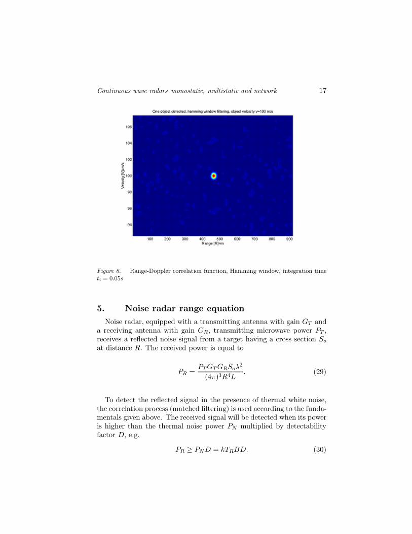
from Equation (27), is presented in Figure 5. It is easy to see the presenceof very high side lobes along the frequency dimension, caused by theboxcar window introduced by integration limits. To decrease side lobelevels, more elaborate time windows (Hamming, Blackman and others)can be used. The windowing can be applied either at the transmissionside (by changing the transmitted signal amplitude) or during signalprocessing. The second approach leads to the concept of unmatchedfiltering, described by the formula

y(r, v) =

ti∫

t=0

w(t)xRx∗

T (t −2r

c)e−j2π(− 2vF

c)t, (28)

where w(t) is a time windowing function [13]. The result of applying theHamming window to range-Doppler correlation processing is presentedin Figure 5. The first side-lobe level is decreased from -13 dB to -60 dB.

Figure 5. Range-Doppler correlation function, boxcar window, integration timeti=0.05 s


Figure 6. Range-Doppler correlation function, Hamming window, integration timeti = 0.05s

5. Noise radar range equation

Noise radar, equipped with a transmitting antenna with gain GT anda receiving antenna with gain GR, transmitting microwave power PT ,receives a reflected noise signal from a target having a cross section So

at distance R. The received power is equal to

PR =PT GT GRSoλ

2

(4π)3R4L. (29)

To detect the reflected signal in the presence of thermal white noise,the correlation process (matched filtering) is used according to the funda-mentals given above. The received signal will be detected when its poweris higher than the thermal noise power PN multiplied by detectabilityfactor D, e.g.

PR ≥ PND = kTRBD. (30)

18

The correlation receiver’s property described above shows that thedetectability factor is equal to

D =Do

tiB. (31)

For medium integration time the time-bandwidth product is limitedby the range migration effect [40]:

tiB ≤c

2Vmax. (32)

Assuming that the maximum target velocity is equal to 3M (1000m/s),the maximum value of the time-bandwidth product is limited to 150,000.The maximum processing gain is then equal to 51.7 dB. The use of awindowing function will decrease this value by a few dB. The maximumdetection range for the noise radar is given by the formula

Rmax = 4

√

PT GT GRSoλ2tt(4π)3LDokT

. (33)

To increase the detection range one can increase the transmittedpower, antenna gain or integration time.

To achieve a longer correlation time it is necessary to incorporaterange and Doppler cell migration effects into the detection process.Let us first consider the range cell migration problem. Assuming con-stant target radial velocity vo, the range to target can be expressed asr = ro + vot. In Equation (27) the target’s velocity influence is limitedonly to the Doppler effect. For a longer integration time it is neces-sary to take into consideration the fact that the time delay of the signalchanges considerably during the integration time. Incorporating timedelay changes the detection process; one can obtain a modified correla-tion expression in the form

y(r, v) =

ti∫

t=0

w(t)xRx∗

T (t − 2r + vt

c)e−j2π(− 2vF

c)t. (34)

The computational complexity required to compute the range-Dopplercorrelation plane is now much higher than the computational cost of cal-culating results using equation (27), where it is necessary to time-scalethe transmitted function. Time scaling may be performed in the timedomain by resampling the transmitted signal or by using a chirp trans-form. For very long integration times it is hard to justify an assumption


of a target’s constant range velocity motion. The target’s range velocitychanges (range acceleration) can cause both velocity cell migration andadditional range cell migration. Proper target detection can be achievedonly when the target’s velocity remains in the velocity resolution cell,which leads to the constraint

ti <

√

2λ

amax, (35)

where amax is the target’s maximum range acceleration. For example,for a 10 cm wavelength and target acceleration of 1g (9.81 m/s), thecoherent integration time is limited to 0.14 s, while for 10 g it is limitatedto 0.045 s. Acceleration may also cause additional range migrations, ifthe integration time exceeds the limit

ti <

√

2∆r

amax=

√

c

Bamax. (36)

To extend the integration time further, it is necessary to introduceacceleration into the target’s motion model. The range to the targetshould now be expressed as r = ro + vot + aot

2/2. The matched fil-ter concept now leads to the three-dimensional range-Doppler-velocitycorrelation function in the form

y(r, v, a) =

ti∫

t=0

w(t)xRx∗

T (t −2r + 2vt + at2

c)e−j2π(−

(2vt+at2)F

c). (37)

Long integration time is important in multibeam radar. The trans-mitting antenna in this type of radar is either sector or omni-directional,and the transmitting gain is at the level of a few dB. The receiver an-tenna should be designed as a multi-beam antenna. Signals from eachbeam are passed to a multi-channel receiver where a correlation processaccording to Equation (37) is performed.

6. Bi-static and multi-static continuous waveradars

Monostatic radar is a radar which has the transmitter and receiverin one place. This idea has many advantages. For example it is easyto use a single clock source for both the transmitter and receiver andthus it is relatively easy to make a fully coherent device. There is noneed to transmit the reference signal to the remote site; the entire pro-cessing can be done locally. The radar can send data to the command

20

and control center at the track level, which requires very low transmis-sion throughput (1-20 kb/s), or on the plot level (10-100 kb/s). Forcontinuous wave radar, the mono-static configuration also has severaldisadvantages. For example, very good separation (usually better than60 dB) between transmitter and receiver antennas is required. Echopower changes as the reciprocal of the fourth power of the range. If theratio between the maximum and the minimum targets’ distance is atthe level of 1000 (e.g. maximum distance 100 km, minimum distance100 m), then the required dynamic range exceeds 120 dB. Additionally,there exist stealth targets, which reflect energy in different directionsthan the direction towards the radar. It is very difficult or even impossi-ble to detect such targets using mono-static radars. The accuracy of thetarget’s position estimation in monostatic radar is limited. The rangeto the target is calculated usually with good accuracy (estimation error1-30 m), but cross-range accuracy is usually very poor (error of a fewkilometers at 100 km distance).

Using the bi-static concept can reduce all of the above mentionedproblems. The spatial separation of the transmitter and receiver anten-nas leads to significant attenuation of the direct path signal. In addition,the near-far target problem is reduced, while the target signal can beexpressed by the formula

PR =PT GT GRSoλ

2

(4π)3R21R

22L

, (38)

where R1 is the transmitter-target distance and R2 is the target-receiverdistance. The required dynamic range for the maximum and minimumtargets’ distance ratio equal to 1000 (e.g. the maximum target’s distancefrom receiver 100 km, the minimum distance 100 m, the transmitter-receiver distance 10 km) is now reduced to 80 db (40 dB smaller than forthe mono-static case). The maximum target detection range is describedby the formula

R1maxR2max =

√

PT GT GRSoλ2tt(4π)3LDokT

. (39)

The bi-static theoretical coverage diagram forms the so-called Cassinicurve, presented in Figure 7. In practice it is not possible to detecttargets in the direction of the transmitter line-of-sight, and practicalbi-static radar coverage is presented in Figure 8.

With the receiving antenna in a different place than the transmit-ting one it is possible to increase the effective radar cross-section ofstealth targets. Increasing the number of receiving antennas and form-ing a multi-static constellation, it is possible to decrease the detection


Figure 7. Bistatic theoretical coverage diagram, detected RCS [dBsm]

losses caused by signal fading, multi-path effects and target scatteringdirectivity. It is also possible to locate and track targets very accuratelyusing the multi-static concept. Expected errors in almost all surveillancespaces are at the level of 1–20 m. Using an adequate number of sensors(4 or more), it is possible to estimate the target’s height, even in thecase when the sensors do not have 3D measurement capabilities.

To use a multi-static configuration, it is necessary to have the referencesignal at each receiving site. The reference signal can be received by thespecial reference channel or can be sent from the transmitter using highthroughput (10-100 Mb/s) digital links.

Multi-static radar is usually combined with the net-centric approachto data exchange. All sensor sites have to be connected by high-through-put, self-configuring data links. The data links should also provide a verystable clock to make all processing coherent, and very accurate time datato synchronize all events in the distributed system.

22

Figure 8. Bistatic coverage diagram — direct illumination attenuation effect, de-tected RCS [dBsm]

7. Target identification in continuous waveradars

Identification of the target is the final stage of radar signal processing.Parameters of the identified target can be displayed on the sensor screenor can be sent to a remote command center. There is no one superioridentification procedure, so identification processes are designed usingdifferent approaches. Almost all of them are based on Doppler processingof the received radar signal.

One widely-used identification method is based on the SAR concept.The radar is mounted on a moving platform. Platform motion is perpen-dicular to the line-of-sight of the fixed radar antenna, and the antennabeam is scanning the target during platform motion. The distance fromthe radar to the selected scatterer is almost a hyperbolic function of time.The Doppler frequency of the target’s signal is then a linear function oftime, and as a result, each echo signal has a chirp form. Applying matchfiltering, it is possible to obtain a high-resolution image of the target.The classical angular resolution of the radar is equal to the product ofthe target’s range and the antenna beam width. For a distance of 10


km and antenna beam width 50 [mrad] the angular resolution is equalto 500 m. Using SAR technology, it is possible to improve resolutionto D/2, where D is the antenna length. Using a low-gain, small sizeantenna it is possible to obtain a sub-meter cross-range resolution and avery detailed image of the target. A SAR image example is presented inFigure 9. The raw radar image used for the SAR processing is presentedin Figure 10.

Figure 9. SAR image of arrow shaped object

Figure 10. Raw radar data of arrow shaped object

In this example, the SAR compression factor was 1000. It is possibleto achieve even higher compression ratios and a better cross-range resolu-tion by using spotlight-SAR. In this mode the radar antenna tracks thetarget and observation time (time-on-target) is significantly enlarged.SAR is often used for air-borne and space-borne remote sensing. It isalso used for ground penetrating radar and for imaging hidden targets.

24

An interesting modification of the above is ISAR (Inverse SyntheticAperture Radar). The ISAR scenario is opposite to the SAR scenario.The radar is now placed in a fixed position and the target changes itsposition in time. The Doppler history of each scatterer on the target’ssurface is different, and the target image is reconstructed using a bankof digital filters matched to the signal originating from each target’sscatterer. This technology is used for ship, airplane and space satelliteimaging. Very often the radar, placed on a moving platform, is observinga moving target. For such a scenario it is possible to combine both ofthe above technologies.

Doppler processing is also used for vehicle and people identification.The identification can be achieved using micro-Doppler analysis. Micro-Doppler vibration analyses are based on detecting Doppler frequencymodulations caused by vibration of the vehicle body resulting from en-gine or gearbox frequencies. Analyzing the Doppler signal originatingfrom the vehicle it is possible to detect all characteristic frequencies,and even to make a mechanical diagnosis of the state of the engine andshafts.

Figure 11. Wire model of human body used for walk Doppler signature analysis

Micro-Doppler analyses can also be used for people identification. Inthat case, it is possible to detect Doppler frequency modulation causedby heartbeats, breathing and body motion (walk, run, head turns etc.).

For people identification, it is also possible to combine micro-Doppleranalyses with ISAR processing. During walk and run, there is a verycharacteristic movement of legs and hands. Making even a very sim-ple “wire-model” of the human body (see Figure 11), it is possible topredict a human Doppler signature. The modeled signature of humanwalk is presented in Figure 12. The signature obtained using a real-life signal, registered in X-band radar, is presented in Figure 13. By


Figure 12. Simulated Doppler signature of human walk - x-axis: time, y-axis:Doppler frequency

Figure 13. Registered Doppler signature of human walk - x-axis: time, y-axis:Doppler frequency

comparing the predicted signature with the recorded one it is possibleto recognize individual behavior, and combining it with heartbeat, walkand breathing analysis it is possible to identify people and even estimatetheir emotional state.

References

[1] B.M. Horton, “Noise-modulated distance measuring system”, Proc. IRE, V0147,pp. 821–828, May 1959.

[2] G.R. Cooper and C.D. McGillem, “Random signal radar”, School Electr. Eng.,Purdue Univ., Final Report, TREE67-11, June 1967.

26

[3] R.M. Naryanan et al., “Design and performance of a polarimetric random noiseradar for detection of shallow buried targets”, Proc. SPIE Meeting on DetectionTechn. Mines, Orlando, April 1995, vol. 2496, pp. 20–30.

[4] I.P. Theron et al., “Ultra-Band Noise Radar in the VHF/UHF Band”, IEEEAP-47, June 1999, pp. 1080–1084.

[5] S.R.J. Axelsson, “On the Theory of Noise Doppler Radar”, Proc. IGARSS 2000,Honolulu, 24-28 July 2000, pp. 856–860.

[6] R. M. Narayanan, Y. Xu, P. D. Hoffmeyer, and J. O. Curtis, “Design, perfor-mance, and applications of a coherent ultra wide-band random noise radar”,Opt. Eng., vol. 37, no. 6, pp. 1855–1869, June 1998.

[7] Y. Xu, R. M. Narayanan, X. Xu, and J. O. Curtis, “Polarimetric processingof coherent random noise radar data for buried object detection”, IEEE Trans.Geosci. Remote Sensing, vol. 39, no. 3, pp. 467–478, Mar. 2001.

[8] R. M. Narayanan and M. Dawood, “Doppler estimation using a coherent ultrawide-band random noise radar”, IEEE Trans. Antennas Propagat., vol. 48, pp.868–878, June 2000.

[9] D. Garmatyuk and R. M. Narayanan, “Ultrawide-band noise synthetic radar:Theory and experiment”, in IEEE Antennas Propagat. Soc. Int. Symp. 1999,vol. 3, Orlando, FL, July 1999, pp. 1764–1767.

[10] D. C. Bell and R. M. Narayanan, “ISAR turntable experiments using a coherentultra wide-band random noise radar”, in IEEE Antennas Propagat. Soc. Int.Symp. 1999, Orlando, July 1999, pp. 1768–1771.

[11] D. J. Daniels, “Resolution of ultra wide-band radar signals”, Proc. Inst. Elec.Eng.-Radar, Sonar Navig., vol. 146, no. 4, pp. 189–194, Aug 1999.

[12] M. E. Davis, “Technical challenges in ultra wide-band radar development fortarget detection and terrain mapping”, in Proc. IEEE 1999 Radar Conf., Boston,MA, April 1999, pp. 1–6.

[13] F. J. Harris, “On the use of windows for harmonic analysis with the discreteFourier transform”, Proc. IEEE, vol. 66, no. 1, pp. 51–83, Jan. 1978.

[14] B. D. Steinberg, D. Carlson, and R. Bose, “High resolution 2-D imaging withspectrally thinned wide-band waveforms”, in Ultra Wideband Short-Pulse Elec-tromagnetics 2, L. Carin and L. B. Felsen, Eds. New York: Plenum , 1995, pp.563–569.

[15] Craig. S.E, Fishbein, W., Rittenbach, O.E., “Continuous-Wave Radar with HighRange Resolution and Unambiguous Velocity Determination”, IRE Trans. MilElectronics, vol. MIL 6. No. 2. April 1962, pp. 153–161.

[16] D. S. Garmatyuk and R. M. Narayanan, “SAR imaging using acoherent ul-trawideband random noise radar”, in Radar Processing, Technology, ond Ap-plications IV, (William I. Miceli, Editor), Proceedings of SPIE Vol. 3810. pp.223–230, Denver, CO, July 1999.

[17] M Soumekh, “Reconnaissance with ultra wideband UHF synthetic apertureradar”, in IEEE Signal Proc. Mag.. Vol. 12, No. 4, pp. 21–40, July 1995.

[18] L. Y. Astanin and A . A. Kostylev, “Ultrawideband Radar Measurements, Anal-ysis and Processing”, The Institution of Electrical Engineers, London, 1997.


[19] Garmatyuk, D.S.; Narayanan, R.M., “SAR imaging using fully random ban-dlimited signals”, Antennas and Propagation Society International Symposium,2000. IEEE Vol. 4 (2000), pp. 1948–1951.

[20] Mogila, A.A.; Lukin, K.A.; Kovalenko, N.P.; Kovalenko, R.P., “Ka-band noiseSAR simulation”, Physics and Engineering of Millimeter and Sub-MillimeterWaves, 2001. The Fourth International Kharkov Symposium, 4–9 June 2001,Volume 1, pp. 441–443.

[21] M. P. Grant, G. R. Cooper, and A. K. Kamal, “A class of noise radar systems”,Proc. IEEE, vol. 51, pp. 1060–1061, July 1963.

[22] R. M. Narayanan, R. D. Mueller, and R. D. Palmer, “Random noise radarinterferometry”, in Proc. SPIE Conf. Radar Processing, Technol. Appl., vol.2845, W. Miceli, Ed., Denver, CO, Aug. 1996, pp. 75–82.

[23] R. M. Narayanan, Y. Xu, P. D. Hoffmeyer, and J. O. Curtis, “Design, perfor-mance, and applications of a coherent ultrawideband random noise radar”, Opt.Eng., vol. 37, no. 6, pp. 1855–1869, June 1998.

[24] R. M. Narayanan and M. Dawood, “Doppler estimation using a coherentultrawide-band random noise radar”, IEEE Trans. Antennas Propagat., vol.48, pp. 868–878, June 2000.

[25] I. P. Theron, E. K. Walton, and S. Gunawan, “Compact range radar cross-section measurements using a noise radar”, IEEE Trans. Antennas Propagat.,vol. 46, pp. 1285–1288, Sept. 1998.

[26] I. P. Theron, E. K. Walton, S. Gunawan, and L. Cai, “Ultrawide-band noiseradar in the VHF/UHF band”, IEEE Trans. Antennas Propagat., vol. 47, pp.1080–1084, June 1999.

[27] L. Guosui, G. Hong, and S. Weimin, “Development of random signal radars”,IEEE Trans. Aerosp. Electron. Syst., vol. 35, pp. 770–777, July 1999.

[28] J. D. Sahr and F. D. Lind, “The Manastash Ridge radar: A passive bistatic radarfor upper atmospheric radio science”, Radio Sci., vol. 32, no. 6, pp. 2345–2358,Nov. 1997.

[29] M. A. Ringer and G. J. Frazer, “Waveform analysis of transmissions of oppor-tunity for passive radar,” in Proc. ISSPA, Brisbane, Australia, Aug. 1999, pp.511–514.

[30] D. S. Garmatyuk and R. M. Narayanan, “Ultra wide-band continuous-wave ran-dom noise arc-SAR”, in IEEE Transactions on Geoscience and Remote Sensing,Volume 40, Issue 12, Dec. 2002, pp. 2543–2552.

[31] Xu Xiaojian and R. M. Narayanan, “FOPEN SAR imaging using UWB step-frequency and random noise waveforms”, IEEE Transactions on Aerospace andElectronic Systems, Volume 37, Issue 4, Oct. 2001, pp. 1287–1300.

[32] S. R. J. Axelsson, “Noise radar using random phase and frequency modula-tion”, Proc. of IEEE International Geoscience and Remote Sensing Symposium(IGARSS) 2003, Volume 7, 21–25 July 2003, pp. 4226–4231.

[33] S. R. J. Axelsson, “Suppressed ambiguity in range by phase-coded wave-forms”, Proc. of IEEE International Geoscience and Remote Sensing Symposium(IGARSS) 2001, Volume 5, 9–13 July 2001, pp. 2006–2009.

[34] K.S. Kulpa, Z. Czekala, “Ground Clutter Suppression in Noise Radar”, Proc.Int. Conf. RADAR 2004, 18–22 October2004, Toulouse, France, p. 236.

28

[35] M.Nalecz, K. Kulpa, A. Piatek, “Hardware/Software Co-designin DSP-BasedRadar and Sonar Systems”, International Radar Symposium 2004 19-21 Maj,Warsaw, Poland, pp. 137–142.

[36] K. Kulpa, “Adaptive Clutter Rejection in Bi-static CW Radar”, InternationalRadar Symposium 2004 19–21 Maj, Warszawa Polska, pp. 61–68.

[37] M. Nalecz, K. Kulpa, R. Rytel-Andrianik, S. Plata, B. Dawidowicz, “Datarecording and processing in FMCW SAR system”, International Radar Sym-posium 2004 19–21 Maj, Warsaw, Poland, pp. 171–177.

[38] K. Kulpa, Z. Czekala, “Short Distance Clutter Masking Effects in Noise Radars”,Proceedings of the International Conference on the Noise Radar Technology.Kharkiv, Ukraine, 21–23 October 2003.

[39] A. Wojtkiewicz, M. Nalecz, K. Kulpa, R. Rytel-Adrianiuk, “A novel Approach toSignal Processing in FMCW Radar”, Bulletin of the Polish Academy of Science,Technical Sciences, Vol. 50, No. 4, Warszawa 2002, pp. 346-359.

[40] K. Kulpa, Z. Czekala, M. Smolarczyk, “Long-Time-Integration SurveillanceNoise Radar”, First International Workshop On The Noise Radar Technology(NRTW 2002), Yalta, Crimea, Ukraine, September 18–20, 2002, pp. 238–243.

[41] K.Kulpa, A.Wojtkiewicz, M.Nalecz, J.Misiurewicz, “The simple analysis methodof nonlinear frequency distortions in FMCW radar”, Journal of Telecommuni-cations and Information Technology, No. 4, 2001, pp. 26–29.

[42] A. Wojtkiewicz, M. Nalecz, K. Kulpa, “A novel approach to signal processing inFMCW radar”, Proc. Int. Conf. on Signals and Electronic Systems ICSES’2000,Ustron, Poland, 17–20 Oct. 2000, pp. 63–68.

[43] Stove A.G., “Linear FMCW radar techniques”, IEE Proceedings-F, Vol. 139,No. 5, Oct. 1992, pp. 343–350.

[44] M. J. Skolnik, “Radar Handbook”, McGraw-Hill Professional; 2nd edition, Jan-uary 1990.

[45] A.Wojtkiewicz, M.Nalecz, K.Kulpa, W.Klembowski, “Use of Polynomial PhaseModeling to FMCW Radar. Part C: Estimation of Target Acceleration inFMCW Radars”, NATO Research and Technology Agency, Sensors and Elec-tronics Technology Symposium on Passive and LPI (Low Probability Of In-tercept) Radio Frequency Sensors, Warsaw, Poland, April 23–25, 2001, paper#40C.

[46] K. Kulpa, “Novel Metchod of Decreasing Influence of Phase Noise on FMCWRadar”, 2001 CIE International Conference on Radar Processing, Oct. 15–18,2001, Beijing, China, pp. 319–323.

continuous wave radars–monostatic, …€¦ · · 2005-07-29abstract radar technology was...

Documents