Continuum Methods 1

John Lowengrub

Dept MathUC Irvine

Membranes, Cells, Tissues

Micro scale•Cell: ~10 micron•Sub cell (genes, large proteins): nanometer

Macro scaleTissues:

billion to 1000 billion cellsor

1—10 centimeter

Processes at cell scale

Signals at sub-cell scale cell aggregation,organ development

•complex micro-structured soft matter

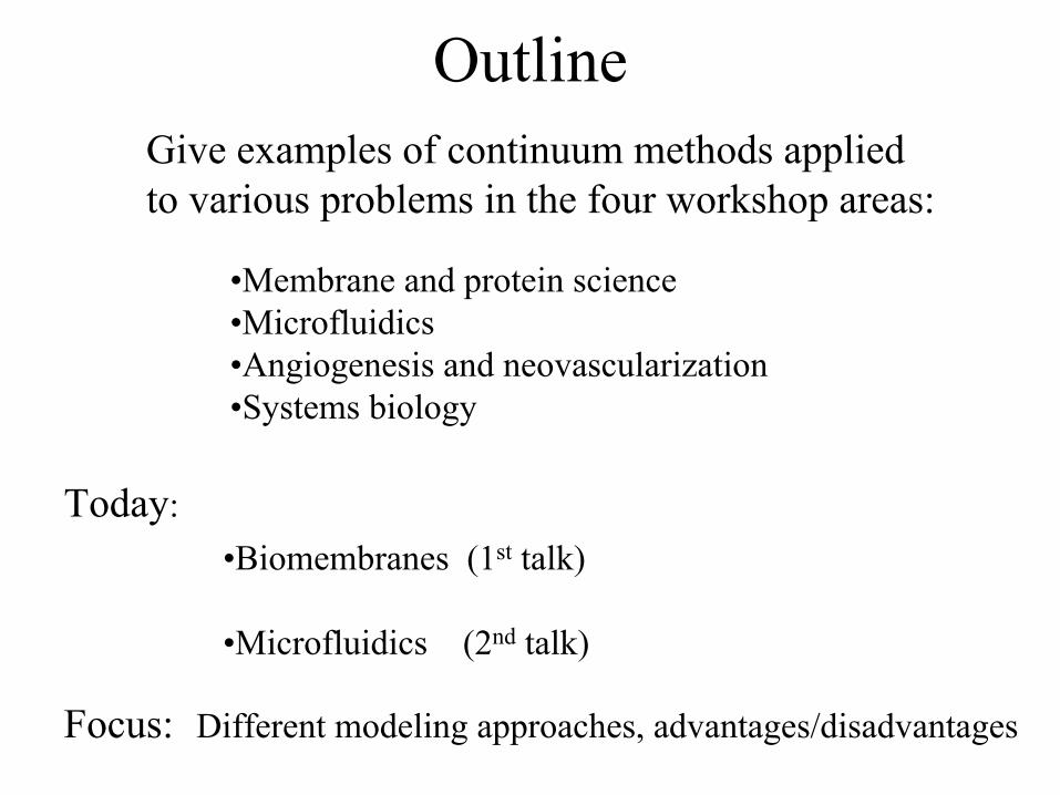
OutlineGive examples of continuum methods appliedto various problems in the four workshop areas:

•Membrane and protein science•Microfluidics•Angiogenesis and neovascularization•Systems biology

Today:•Biomembranes (1st talk)

•Microfluidics (2nd talk)

Focus: Different modeling approaches, advantages/disadvantages

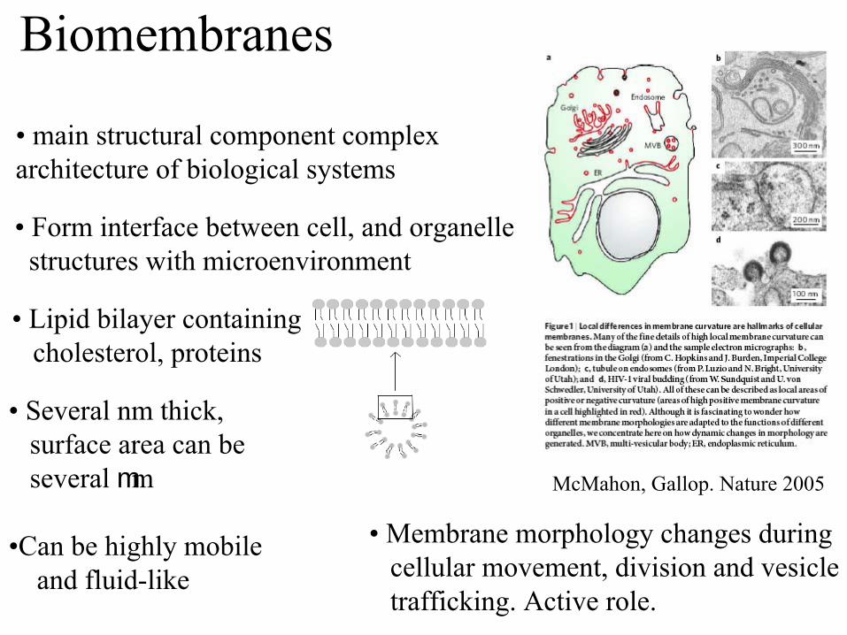
Biomembranes

• Form interface between cell, and organelle structures with microenvironment

• Lipid bilayer containingcholesterol, proteins

• main structural component complex architecture of biological systems

McMahon, Gallop. Nature 2005

• Membrane morphology changes duringcellular movement, division and vesicletrafficking. Active role.

• Several nm thick, surface area can beseveral mm

•Can be highly mobileand fluid-like

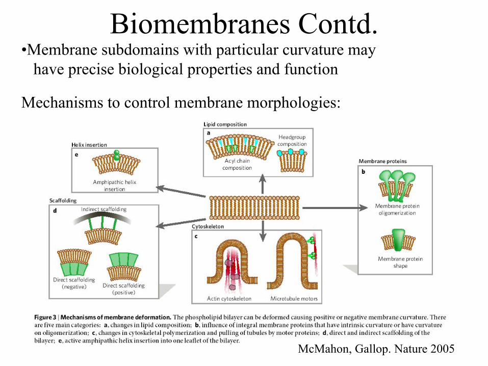
Biomembranes Contd.•Membrane subdomains with particular curvature may

have precise biological properties and function

Mechanisms to control membrane morphologies:

McMahon, Gallop. Nature 2005

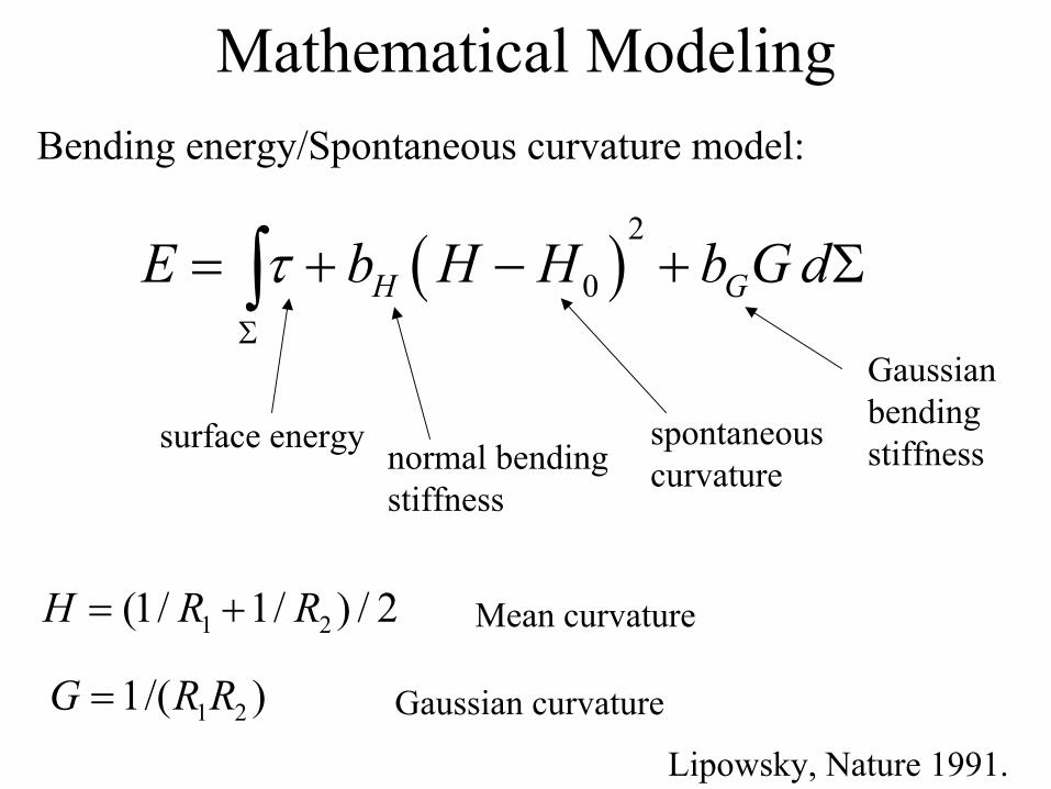
Mathematical ModelingBending energy/Spontaneous curvature model:

( )2

0H GE b H H b G dτΣ

= + − + Σ∫

surface energy normal bendingstiffness

spontaneouscurvature

Gaussianbendingstiffness

1 2(1/ 1/ ) / 2H R R= + Mean curvature

1 21/( )G R R= Gaussian curvature

Lipowsky, Nature 1991.

Constraints

0A d AΣ

= Σ =∫•Area constraint

(exchange of lipids with surrounding microenvironment is typically very slow)

•Volume constraint

0( ) 1/ 3Vol d VΣ

Σ = • Σ =∫ x n

(limited osmosis, can be controlled however)

Morphology: Minimization of E subject to above constraints.

Related Problems

•Willmore flow

•Surface diffusion in materials

•Image processing

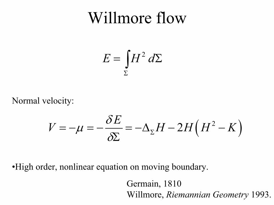
Willmore flow

2E H dΣ

= Σ∫

Normal velocity:

( )22EV H H H Kδµδ Σ= − = − = −∆ − −Σ

•High order, nonlinear equation on moving boundary.

Germain, 1810Willmore, Riemannian Geometry 1993.

Surface diffusion in materials

( ),E H dτΣ

= Σ∫ n

n Normal vector (reflects crystalline anistropy)

( )2

2, ( )2

H Hδτ γ θ= +nExample (2D):

Then, chemical potential given by (2D)

( ) ( )2 3( ) ''( ) ssE H H Hδµ γ θ γ θ δδ

= = − + + +Σ

Normal velocity:ssV µ=

DiCarlo, Gurtin, Podio-Duidugli, SIAM J. Appl. Math. (1992);Gurtin,Jabbour, Arch. Rat. Mech. Anal. (2002); Spencer, Phys. Rev. E (2004)

6th order system!

Wulff Shapes for 4-fold Anisotropy

Wulff Shapes:

Nonphysical“ears” form for

(given enclosed area)

increasing

increasing

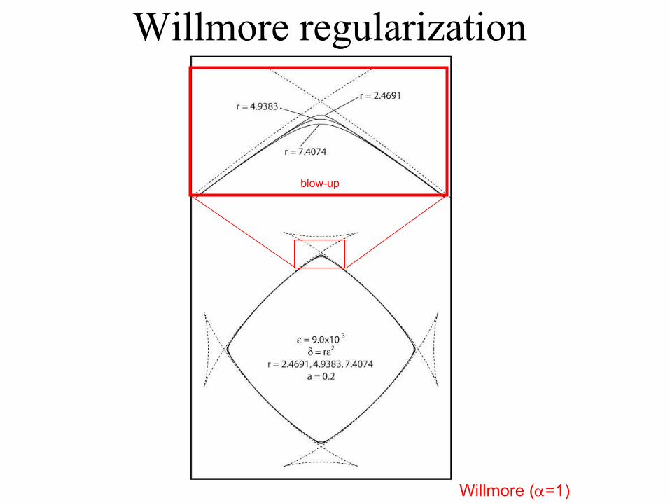
Willmore regularization

Willmore (α=1)

blow-up

Image processing

Clarenz, et al, C. A. Geom.Design 2004

Xu, Pan, C.A.D. 2006

Difficulties

V HΣ−∆∼

Numerical stiffness:

4t s∆ ≤ ∆

•Surface diffusion V HΣ= −∆

Computational Methods

•Sharp interface/front-tracking

•Level-set methods/front capturing

•Phase-field methods/front capturing

with Willmore regularization2V HΣ

∆∼

Sharp interface methods

Implicit discretizations, marker-point redistribution

Mayer, Simonett. 2001

Bansch, Morin, Nochetto JCP 2005

•Small scale decomposition (2D, Axisymmetric). Hou, Lowengrub, Shelley JCP 1994

•To overcome stiffness:

Surface diffusion Axisymmetric Willmore

t

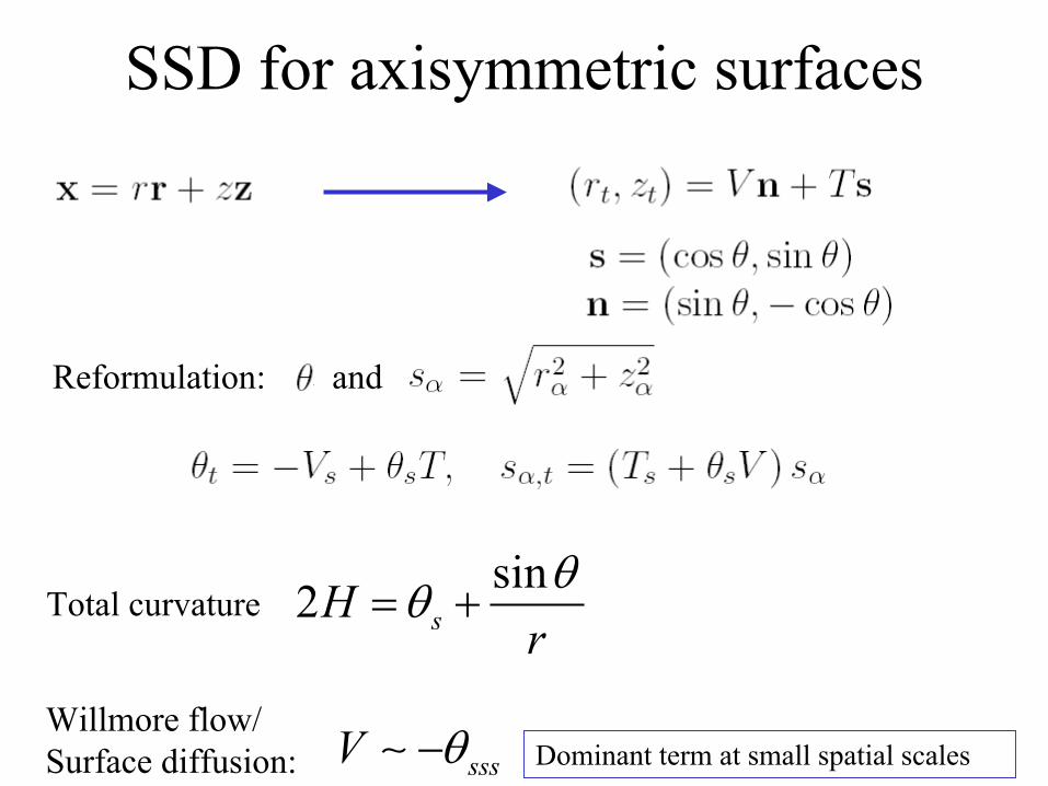
SSD for axisymmetric surfaces

Reformulation: and

Willmore flow/Surface diffusion: sssV θ−∼ Dominant term at small spatial scales

Total curvaturesin2 sH

rθθ= +

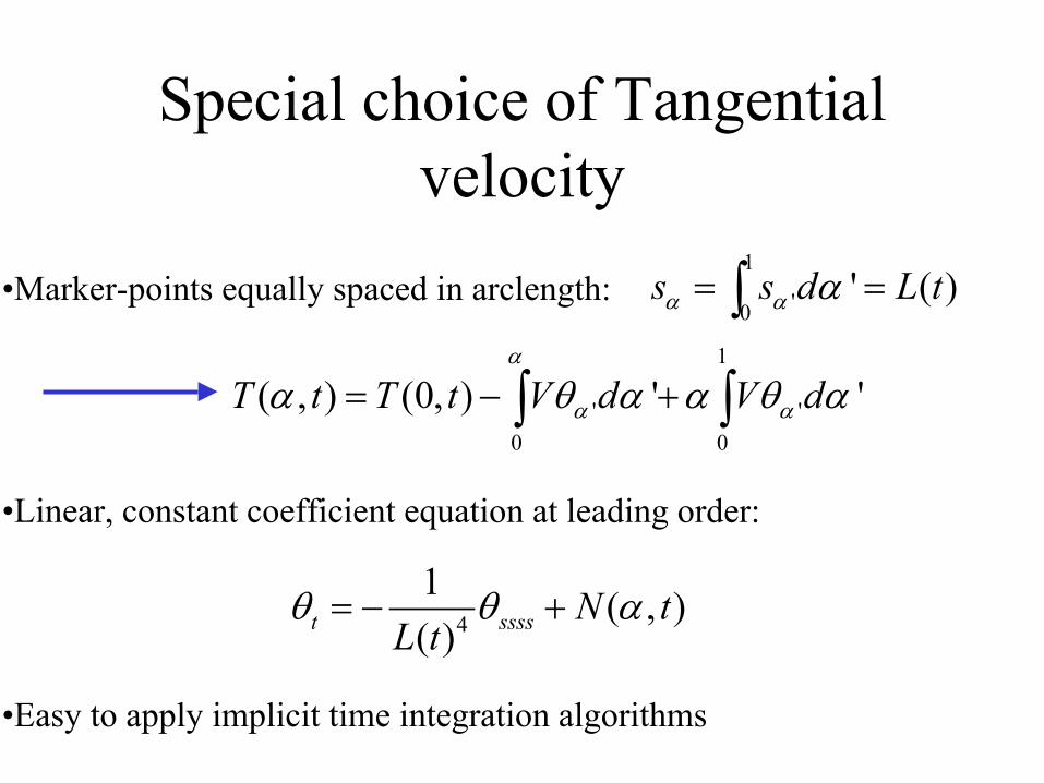
Special choice of Tangential velocity

•Marker-points equally spaced in arclength:1

'0' ( )s s d L tα α α= =∫

1

' '0 0

( , ) (0, ) ' 'T t T t V d V dα

α αα θ α α θ α= − +∫ ∫

•Linear, constant coefficient equation at leading order:

4

1 ( , )( )t ssss N t

L tθ θ α= − +

•Easy to apply implicit time integration algorithms

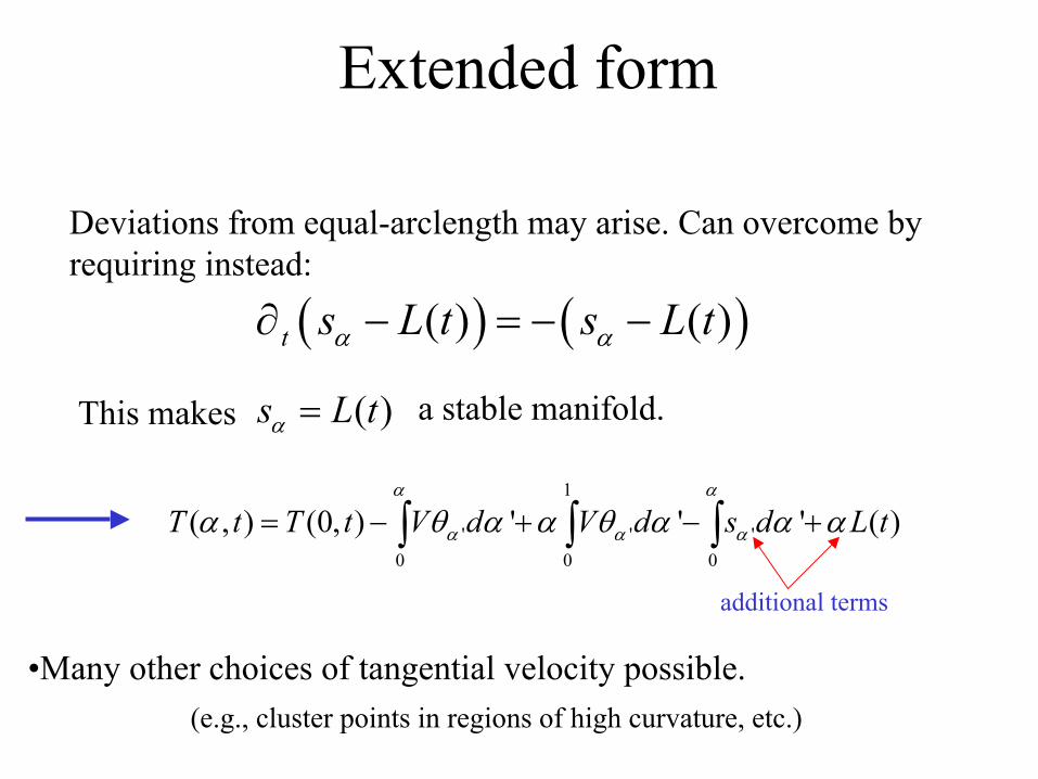
Extended form

Deviations from equal-arclength may arise. Can overcome byrequiring instead:

( ) ( )( ) ( )t s L t s L tα α∂ − = − −

This makes ( )s L tα = a stable manifold.

1

' ' '0 0 0

( , ) (0, ) ' ' ' ( )T t T t V d V d s d L tα α

α α αα θ α α θ α α α= − + − +∫ ∫ ∫

•Many other choices of tangential velocity possible.(e.g., cluster points in regions of high curvature, etc.)

additional terms

3D

Finite element approach.

Update:

Bansch, Morin, Nochetto JCP 2005.

Solve:

By:

Using C0 elements.

Evaluated on current (time n) surface

Extension to Willmore flowBurger, Voigt et al (2006)

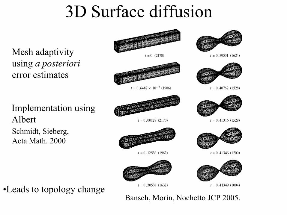
3D Surface diffusion

Bansch, Morin, Nochetto JCP 2005.

Mesh adaptivityusing a posteriorierror estimates

Implementation usingAlbertSchmidt, Sieberg,Acta Math. 2000

•Leads to topology change

Level-set methods

{ }( ) | ( , ) 0t tφΣ = =x x

•Interface capturing.

| | 0t extVφ φ+ ∇ =

•Interface moves with speed V:

extVwhere is an extension of V off Σ

Osher, Sethian 1988

Droske, Rumpf IFB 2004

Willmore flow.

weighted meancurvature •Semi-implicit discretization

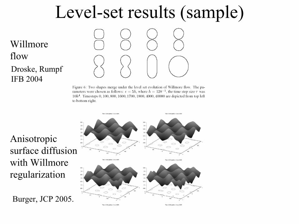
Level-set results (sample)Willmoreflow

Anisotropicsurface diffusionwith Willmoreregularization

Burger, JCP 2005.

Droske, Rumpf IFB 2004

Phase-field methodsc is a smooth order parameter

y

c = 0.5(Γ)

y

xx

y=const cross-section

Why Phase-field?

• Allows the easy capture of interface dynamics.

• Avoid explicit tracking.• Easy to add more physics (e.g., elasticity, multiple

phases).

• Downside: introduce finite thickness.diffuse interface

Phase-field Willmore Problem

Qiang Du et al, A phase field formulation of the Willmore problem, Nonlinearity (2005).

Du et al. showed rigorous asymptotic convergence ( ) of solutions of

to solutions of the classical Willmore problem

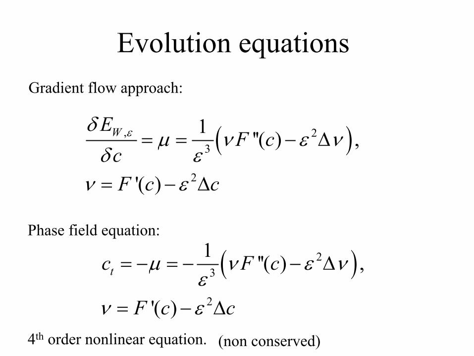
Evolution equationsGradient flow approach:

( ), 23

2

1 ''( ) ,

'( )

WEF c

cF c c

εδµ ν ε ν

δ εν ε

= = − ∆

= − ∆

Phase field equation:

( )23

2

1 ''( ) ,

'( )

tc F c

F c c

µ ν ε νε

ν ε

= − = − − ∆

= − ∆4th order nonlinear equation. (non conserved)

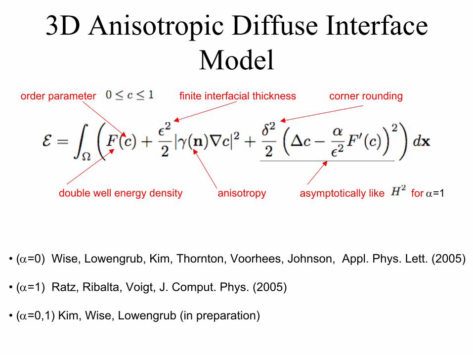
3D Anisotropic Diffuse Interface Model

• (α=0) Wise, Lowengrub, Kim, Thornton, Voorhees, Johnson, Appl. Phys. Lett. (2005)

• (α=1) Ratz, Ribalta, Voigt, J. Comput. Phys. (2005)

• (α=0,1) Kim, Wise, Lowengrub (in preparation)

double well energy density

order parameter finite interfacial thickness corner rounding

anisotropy asymptotically like for α=1

Evolution: 6th-order Cahn-Hilliard Eqn

Asymptotic convergence to the sharp interface surface diffusion model?

diagonal anisotropymatrix

mass conservation:M = 1, bulk diff.; M = c(1-c), surface diff.

linear biharmonicfor α = 0

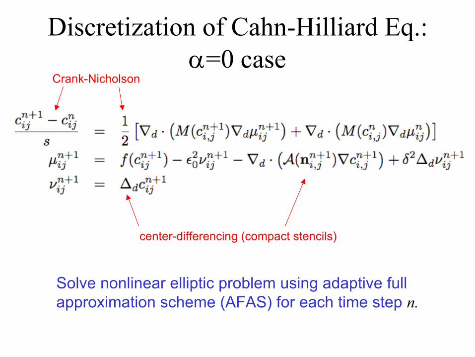
Discretization of Cahn-Hilliard Eq.: α=0 case

Crank-Nicholson

center-differencing (compact stencils)

Solve nonlinear elliptic problem using adaptive full approximation scheme (AFAS) for each time step n.

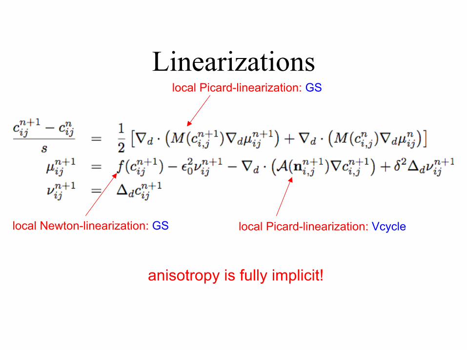
Linearizationslocal Picard-linearization: GS

local Newton-linearization: GS local Picard-linearization: Vcycle

anisotropy is fully implicit!

Details• Mild solvability time-step restriction (being remedied)

• No time-step restriction owing to anisotropy

• Tests indicate 2nd order accuracy method (c, a posteriori in l2)

•J.S. Kim, K. Kang, and J.S. Lowengrub, Conservative multigrid methods for Cahn-Hilliard fluids, J. Comput. Phys., (2004)

•Wise et al., Appl. Phys. Lett. (2005) (QD self assembly)

•Kim, Wise, Lowengrub, Adaptive Method for Strong Anisotropy (in preparation)

30% volume fraction

Uniform mesh

Adaptive mesh

4107×

time

Num

ber of mesh points

7e+04

Isotropic Spinodal Decomposition (a=0, δ=0)

• base level = 642

• 2 levels of refinement• effective 2562

1/6 cost (long times)

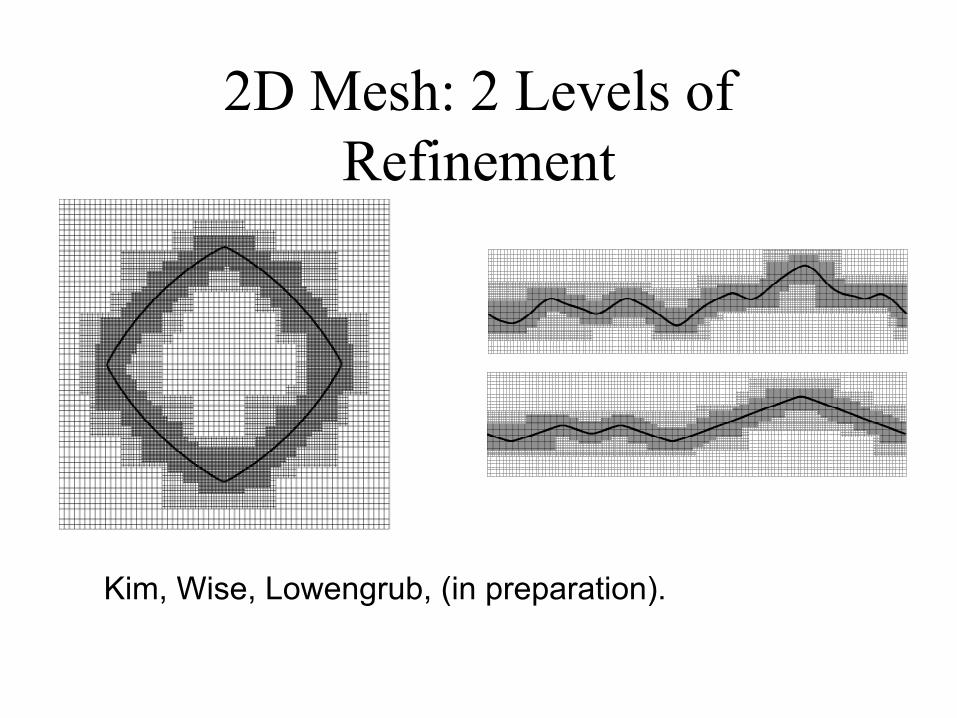
2D Mesh: 2 Levels of Refinement

Kim, Wise, Lowengrub, (in preparation).

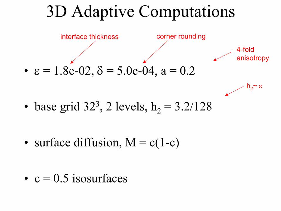
3D Adaptive Computations

• ε = 1.8e-02, δ = 5.0e-04, a = 0.2

• base grid 323, 2 levels, h2 = 3.2/128

• surface diffusion, M = c(1-c)

• c = 0.5 isosurfaces

interface thickness corner rounding

4-foldanisotropy

h2~ ε

Anisotropic surface energy + Willmore regularization

•Evolution to Wulff shape

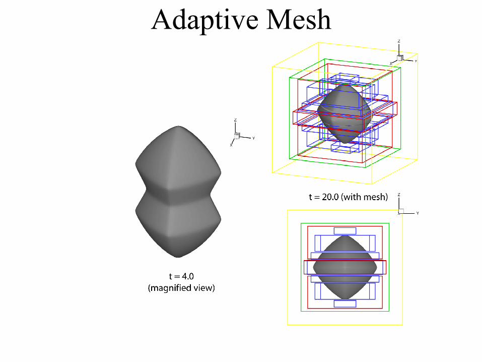
Adaptive Mesh

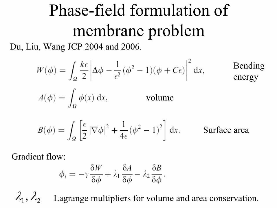
Phase-field formulation of membrane problem

Bendingenergy

volume

Surface area

Du, Liu, Wang JCP 2004 and 2006.

Gradient flow:

1 2,λ λ Lagrange multipliers for volume and area conservation.

Numerical methods•Implicit time discretization,

•Discrete energy law,

•Periodic BC, pseudo-spectral methods

•Evolution to adiscocyte

•Evolutionto a torus

Du, Liu, WangJCP 2006

Further directions•Effects of fluid flow

Du et al. for single-component membranes (to appear)Lowengrub et al for multicomponent membranes

(in progress)

•Multicomponent membranesMore than one lipid component

Baumgart, Hess, WebbNature 2003

Du et al., phase-field models Lowengrub, Voigt et al., sharp interface models