Abstract. Contour integration in low-level vision isbelieved to occur based on lateral interaction betweenneurons with similar orientation tuning. How suchinteractions could arise in the brain has been an openquestion. Our model suggests that the interactions canbe learned through input-driven self-organization, i.e.,through the same mechanism that underlies many otherdevelopmental and functional phenomena in the visualcortex. The model also shows how synchronized firingmediated by these lateral connections can represent thepercept of a contour, resulting in performance similar tothat of human contour integration. The model furtherdemonstrates that contour integration performance candiffer in different parts of the visual field, depending onwhat kinds of input distributions they receive duringdevelopment. The model thus grounds an importantperceptual phenomenon onto detailed neural mecha-nisms so that various structural and functional proper-ties can be measured and predictions can be made toguide future experiments.

1 Introduction

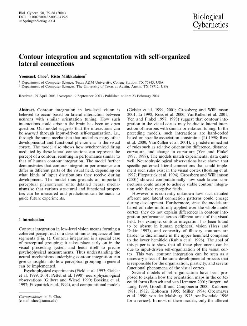
Contour integration in low-level vision means forming acoherent percept out of a discontinuous sequence of linesegments (Fig. 1). Contour integration is a special caseof perceptual grouping; it takes place early on in thevisual processing system and lends itself to precisepsychophysical measurements. Thus understanding theneural mechanisms underlying contour integration cangive us insights into how perceptual grouping in generalcan be implemented.

Psychophysical experiments (Field et al. 1993; Geisleret al. 1999, 2001; Pettet et al. 1998), neurophysiologicalobservations (Gilbert and Wiesel 1990; Bosking et al.1997; Fitzpatrick et al. 1994), and computational models

(Geisler et al. 1999, 2001; Grossberg and Williamson2001; Li 1998; Ross et al. 2000; VanRullen et al. 2001;Yen and Finkel 1997, 1998) suggest that contour inte-gration in the visual cortex may be due to lateral inter-action of neurons with similar orientation tuning. In thepreceding models, such interactions are hard-codedbased on specific association constraints (Li 1998; Rosset al. 2000; VanRullen et al. 2001), a predetermined setof rules such as relative orientation difference, distance,curvature, and change in curvature (Yen and Finkel1997, 1998). The models match experimental data quitewell. Neurophysiological observations have shown thatspecific patterned lateral connections that could imple-ment such rules exist in the visual cortex (Bosking et al.1997; Fitzpatrick et al. 1994). Grossberg and Williamson(2001) showed computationally how such lateral con-nections could adapt to achieve stable contour integra-tion with fixed receptive fields.

However, it is currently unknown how such detailedafferent and lateral connection patterns could emergeduring development. Furthermore, since the models arebased on rules uniformly applied over the whole modelcortex, they do not explain differences in contour inte-gration performance across different areas of the visualfield. For example, contour integration has been foundto be absent in human peripheral vision (Hess andDakin 1997), and convexity of illusory contours areharder to discriminate in the upper hemifield comparedto the lower hemifield (Rubin et al. 1996). The goal ofthis paper is to show that all these phenomena can bedue to input-driven self-organization of the visual cor-tex. This way, contour integration can be seen as anecessary effect of the same developmental process thatis responsible for the organization, plasticity, and severalfunctional phenomena of the visual cortex.

Several models of self-organization have been pro-posed to explain how the orientation maps in the cortexcould form (Bartsch and van Hemmen 2001; Burger andLang 1999; Goodhill and Cimponeriu 2000; Kohonen1981, 1982; Kohonen 1995; Miller 1994; Obermayeret al. 1990; von der Malsburg 1973; see Swindale 1996for a review). In most of these models, only the afferent

Correspondence to: Y. Choe(e-mail: choe@tamu.edu)

Biol. Cybern. 90, 75–88 (2004)DOI 10.1007/s00422-003-0435-5� Springer-Verlag 2004

Contour integration and segmentation with self-organizedlateral connections

Yoonsuck Choe1, Risto Miikkulainen2

1 Department of Computer Science, Texas A&M University, College Station, TX 77843, USA2 Department of Computer Sciences, The University of Texas at Austin, Austin, TX 78712, USA

Received: 29 April 2003 /Accepted: 9 September 2003 / Published online: 23 February 2004

connections self-organize while the lateral interactionsare represented as a fixed, uniform interaction kernel. Inthose models where the lateral connections adapt aswell, the final connectivity pattern is elongated, but notpatchy like the patterns in the visual cortex. Therefore,such models cannot account for functional phenomenathat depend on the specific patterns of lateral connec-tions. With this goal in mind, we recently developed amodel with explicit self-organizing lateral connections,showing that patches of strong lateral connections de-velop between neurons with similar orientation prefer-ence, and that these connections can serve as afoundation for segmentation and binding (RF-SLIS-SOM, or Receptive Field Spiking Laterally Intercon-nected Synergetically Self-Organizing Map) (Bednar andMiikkulainen 2000b; Choe and Miikkulainen 1998;Miikkulainen et al. 1997; Sirosh 1995; Sirosh et al. 1996;Sirosh and Miikkulainen 1997). Self-organization oflaterally connected maps is the first main principle of thecontour integration model presented in this paper.

Patterned lateral interactions are strongly believed tocontribute to contour integration, but how does the vi-sual system represent a contour as a coherent object withits neural activity? A separate line of research has pro-duced a possible answer to this question. Experimentshave shown that feature binding and segmentation in thevisual system may be based on temporal coding pro-duced by synchronous and desynchronous populationactivity (Eckhorn et al. 1988; Engel et al. 1991; Grayand Singer 1987; Gray et al. 1989 (see Singer and Gray1995; Gray 1999; and Singer 1999 for a review)). Locallysynchronous firing has been observed, for example, inthe visual cortex of cats and monkeys. Recordings ofsingle-unit activities, multiunit activities (MUAs), andlocal field potentials (LFPs) in different areas of the vi-sual cortex were taken, and neurons with nonoverlap-ping receptive fields were found most likely to besynchronized when the receptive field properties weresimilar or when the firing represented global stimulusproperties. Computational models also demonstratedthat such behavior could be obtained in a network ofneurons with temporal dynamics (Eckhorn et al. 1990;Gerstner 1998; Grossberg and Grunewald 1997; Hornand Opher 1998; Reitboeck et al. 1993; von derMalsburg 1986, 1987; von der Malsburg and Buhmann1992; Wang 1995, 1996, 2000). Therefore, segmentation

and binding by synchronized firing is the second mainprinciple of our contour integration model.

In this paper, the above two principles are unified intoa single model. We demonstrate that the orientationmap and the lateral connections self-organize so that thefunctional statistics of lateral connections become simi-lar to edge co-occurrence statistics in natural images.These connections mediate synchronized firing of neu-rons, so that the contour integration performance of themodel closely matches psychological data. This way, themodel (i) shows how the circuitry for contour integra-tion could arise from general self-organization mecha-nisms in the brain, (ii) provides further computationalevidence for synchronization as the substrate for seg-mentation and binding, and (iii) grounds an importantperceptual grouping phenomenon on a detailed neuralarchitecture, where various functional properties can bemeasured and predictions made to guide future experi-ments.

2 Model description

2.1 Motivation and overview

The contour integration model is based on the RF-SLISSOM model of self-organization and segmentationin the primary visual cortex Choe and Miikkulainen(1998). In this model, each cortical neuron receivesafferent connections from the input layer and lateralexcitatory and inhibitory connections from neighboringneurons in the cortex. The connection strengths self-organize based on correlations in the activity. In the finalordered map, the lateral excitation has a short range andcauses neurons responding to the same connected inputobject to fire synchronously, effectively binding thespikes into a single coherent representation. The lateralinhibitory connections have a long range and establishcompetition between representations of differentobjects.1 Neurons representing different objects fire atdifferent times, and the input is thereby segmented intodifferent objects.

This previous model showed how self-organizationand segmentation could be achieved in a single unifiedframework. The lateral interactions play a crucial role inboth behaviors: they establish competition that drivesself-organization, and they establish desynchronizationthat drives segmentation. The model did not include anylong-range excitatory connections because they were notfound necessary to model the above behaviors. How-ever, it turns out that such a parsimonious model cannotaccount for filling-in phenomena such as contour inte-gration. The network has to be able to bind togetherrepresentations that are separated by gaps: that is, it has

Fig. 1. Contour integration task. This figure shows a typical inputimage used in psychophysical experiments on contour integration.Human subjects are instructed to find the longest continuous contourconsisting of separate line segments embedded in a background ofrandomly oriented distractors. In this example, the contour consists ofsix segments, running diagonally from middle left to bottom right

1 Although long-range connections in the cortex appear to bemostly excitatory, their effect can be inhibitory through inhibitoryinterneurons (Grinvald et al. 1994; Hata et al. 1988; Hirsch andGilbert 1991; Weliky et al. 1995). RF-SLISSOM abstracts suchinterneurons and models the overall inhibitory effect as oneconnection.

76

to have long-range excitatory connections that linktogether the representations of the different segments ofa fragmented contour.

The model is extended in this paper with such long-range excitatory connections (Fig. 2). The extendedmodel is called PGLISSOM (or Perceptual GroupingLISSOM Choe 2001). The cortical network is dividedinto two separate components: MAP1 and MAP2.MAP1 is similar to the RF-SLISSOM cortex withshort-range excitatory and long-range inhibitory con-nections. This map has the task of driving the self-organization of the network into an ordered map.MAP2 performs the task of long-range segmentationand binding, with long-range excitatory connectionsthat perform contour integration and long-rangeinhibitory connections that implement segmentation ofseparate objects. The two maps are assumed to beoverlaid in one cortical network: such a functionalspecialization across laminar layers of the visual cortexis consistent with known neuroanatomical data fromlayers IV, VI, and II/III of the visual cortex (seeGrossberg and Williamson 2001). In other words, themodel is based on the hypothesis that some of theneurons in each cortical column are involved in estab-lishing and maintaining organization, whereas othersperform visual segmentation and binding.

2.2 Neuron model

The details of the neuron model are illustrated inFig. 2a. Each connection is a leaky integrator thatperforms exponentially decayed summation of incomingspikes (i.e., convolution with an exponential kernel,Eckhorn et al. 1990):

sðtÞ ¼Xt

n¼0xðt � nÞe�kn ; ð1Þ

where sðtÞ is the current decayed sum at time step t,xðt � nÞ is the input spike (either 0 or 1) n time steps inthe past, and k is the decay rate. Different types ofconnections have distinct decay rates: ke for excitatoryand ki for inhibitory lateral connections, and kc forintracolumnar connections. The sum can be defined in acomputationally more practical form as a recurrenceequation, which is used in the current implementation:

sðtÞ ¼ xðtÞ þ sðt � 1Þe�k ; ð2Þwhere sðtÞ and sðt � 1Þ are the current and previousdecayed sums, xðtÞ is the current input spike and k is thedecay rate (Eckhorn et al. 1990). The leaky integratormodels the postsynaptic potential (PSP) that decaysexponentially over time in biological neurons. Byadjusting the decay rate k, the synapse can function aseither a coincidence detector or as a temporal integrator.When the synaptic decay rate is high, the neuron canonly fire when there is a sufficient number of inputscoming in from many synapses simultaneously. On theother hand, when the decay rate is low, the neuronaccumulates the input. Thus presynaptic neurons canhave a lingering influence on the postsynaptic neuron.By varying the decay rates for different types of con-nections, the relative time scales of the different con-nection types can be controlled to obtain desirablesynchronization behavior.

The spike generator compares the input to a thresh-old and decides whether to fire a spike. The threshold isdynamic, depending on the previous firing activity at the

Fig. 2a, b. Overview of the PGLISSOM model. a Neuron model.Leaky integrators at each synapse perform decayed summation ofincoming spikes, and the outgoing spikes are generated by comparingthe sum of weighted sums to the dynamic spiking threshold. Fourtypes of inputs contribute to the activity: afferent, excitatory lateral,inhibitory lateral, and intracolumnar connections. The dynamicthreshold consists of the base threshold hbase, the absolute refractorycomponent habs, and the relative refractory component hrel. b Overall

organization of the network. The cortical network consists of twolayers (or maps): MAP1 has short-range excitation and long-rangelateral inhibition and drives the self-organization of the model. InMAP2, both excitation and inhibition have a long range, establishingbinding and segmentation. Both maps receive input from a modelretina, and neurons in the vertically corresponding locations on thetwo maps are connected via intracolumnar connections representing acortical column

77

neuron, in order to model the refractory period and toimprove synchronization. It consists of three terms:

hðtÞ ¼ hbase þ habsðtÞ þ shrelðtÞ ; ð3Þ

where hbase is the base threshold, habsðtÞ implements theabsolute refractory period during which the neuroncannot fire, hrelðtÞ implements the relative refractoryperiod during which firing is possible but requiresextensive input, and s is a scaling constant. The absoluterefractory component habsðtÞ is defined as:

habsðtÞ ¼ 1 if yðt � iÞ ¼ 1 for any i � jabs

0 otherwise ,

�ð4Þ

where jabs determines the length of the absolute refrac-tory period and yðtÞ represents whether a spike occurredat time t:

yðtÞ ¼HðrðtÞ � hðt � 1ÞÞ ; ð5Þ

where Hð�Þ is the Heaviside step function, rðtÞ is theweighted input sum (7), and hðt � 1Þ is the dynamicthreshold. The relative refractory component hrelðtÞ isimplemented as an exponentially decayed sum of theoutput spikes (Fig. 2a), i.e., a leaky integrator similar tothe leaky synapses:

hrelðtÞ ¼ yðtÞ þ hrelðt � 1Þe�krel ; ð6Þ

where krel is the decay rate.Eckhorn et al.(1990) and Reitboeck et al. (1993) de-

scribed a similar dynamic thresholdmechanism consistingof hbase and hrel only. The absolute refractory period wasincluded in our model to ensure that the neurons did notfire too rapidly. An added benefit is that synchronizationis more robust against noise (Choe 2001).

2.3 Network activation and learning

The organization of the network is shown in Fig. 2b.The input ri;jðtÞ to the spike generator of the corticalneuron (in each map) at location (i; j) at time t consistsof (i) the input from a fixed-size receptive field in theretina2 centered at the location corresponding to theneuron’s location in the cortical network, (ii) fromneurons around the same relative location in theopposite map, (iii) excitation, and (iv) inhibition fromneighboring neurons in the same map:

ri;jðtÞ ¼ g�caX

r1;r2

nr1;r2lij;r1r2

þ ccX

p1;p2

fðt � 1Þp1;p2mij;p1p2

þ ceX

k;l

gklðt � 1ÞEij;kl

� ciX

k;l

gklðt � 1ÞIij;kl

�; ð7Þ

where ca; cc, ce, and ci are, respectively, the relativestrengths of the afferent, intracolumnar, and excitatoryand inhibitory lateral contributions, nr1;r2 is the inputlevel of retinal neuron (r1; r2), lij;r1r2 is the correspondingafferent connection weight, fp1;p2 is the decayed sum ofspikes of the cortical neuron (p1; p2) of the other corticalmap, mij;p1p2 is the corresponding intracolumnar connec-tion weight, gklðt � 1Þ is the decayed sum of spikesfrom the map neuron (k; l) at time t � 1, Eij;kl is thecorresponding excitatory and Iij;kl the inhibitory lateralconnection weight, and gð�Þ is a piecewise linearapproximation of the sigmoid function that squashesthe net input sum between 0.0 and 1.0:

gðxÞ ¼0 if x < d1 if x > bx�db�d otherwise ;

8<

: ð8Þ

where d is the threshold and b is the ceiling.The inputs to the model consist of activation patterns

with activation values ranging between 0 and 1. A fixedsuch input is presented on the retina at each iterationand the cortical neurons are allowed to generate andexchange spikes. After several iterations, the short-termspiking rate of the neurons in a small window is calcu-lated:

V ðtÞ ¼ savgV ðt � 1Þ þ ð1� savgÞyðtÞ ; ð9Þ

where savg is the window size, V ðt � 1Þ is the previousaverage firing rate, and yðtÞ is the output spike at time t.The afferent, lateral, and intracolumnar weights are thenmodified according to the normalized Hebbian learningrule:

wij;mnðtÞ ¼wij;mnðt � 1Þ þ aVijðtÞVmnðtÞPij ½wij;mnðt � 1Þ þ aVijðtÞVmnðtÞ�

; ð10Þ

where wij;mnðtÞ is the connection weight from neuronðm; nÞ to ði; jÞ, wij;mnðt � 1Þ is the previous weight, a is thelearning rate (aa for afferent, ac for intracolumnar, ae forexcitatory, and ai for inhibitory connections), and VijðtÞand VmnðtÞ are the average spiking rates of the neurons.

This process of weight adaptation is repeated withinputs at random locations and orientations, and theneurons gradually become sensitive to particular orien-tations at particular locations, resulting in a global re-tinotopic orientation map similar to that found in thevisual cortex. The self-organized map will then syn-chronize and desynchronize the firing of neurons toindicate binding and segmentation of visual features todifferent objects present in the scene. The lateral con-nections that survive connection death play an impor-tant role in this process by mediating synchronizationand desynchronization among populations of neurons.

3 Experiments

A Stacked RF-SLISSOM network with a 46� 46 retinaand a 136� 136 cortex was trained for 40,000 itera-tions with straight elongated Gaussian bars at random

2 The preprocessing in the retinal ganglion cells and lateralgeniculate nucleus (LGN) was bypassed for simplicity.

78

locations in the retina. Although natural images could inprinciple be used as well (Bednar 2002), such abstractinput is computationally more efficient while stillrepresenting the essential local features of naturalstimuli after the edge detection and enhancementmechanisms in the retina and LGN. During eachtraining presentation, the network was allowed to settlefor 15 time steps (through Eq. 7.) and all connectionsexcept the inhibitory lateral connections in MAP2 wereupdated according to Eq. 10. The fixed inhibition inMAP2 provides a baseline similar to global inhibition inother cortical models (Eckhorn et al. 1988; Kammenet al. 1989; Terman and Wang 1995; von der Malsburgand Buhmann 1992; Wang 1995, 1996, 2000): it allowsinput elements to be segmented by default, unless lateralexcitation binds them together. The details of the modeland the simulation details are given in the Appendix.

3.1 Orientation map and functional connection statistics

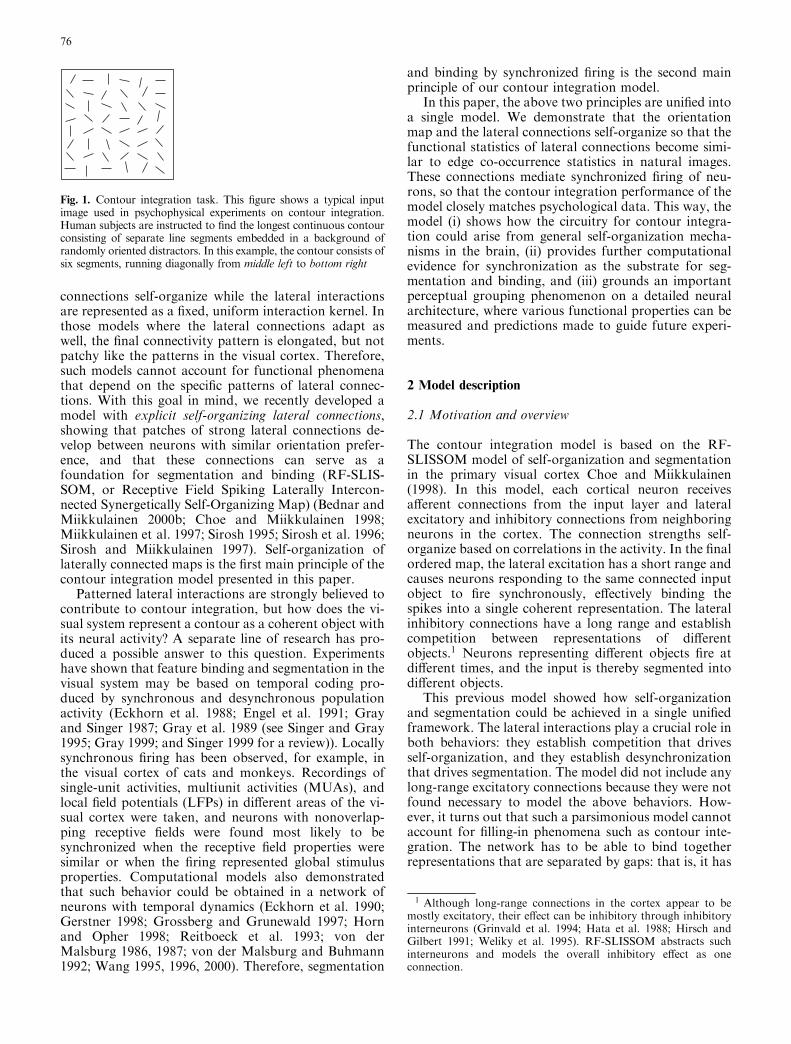
A well-formed orientation map emerged in the trainingprocess (Fig. 3). The map is qualitatively similar to theorientation map in the primary visual cortex withfeatures such as linear zones where orientation prefer-ence changes continuously along one direction, pinwheelcenters around which a full 360� of orientation prefer-ences can be observed, and fractures where orientationpreference changes abruptly (Blasdel 1992; Blasdel andSalama 1986). Because of the intracolumnar connec-tions, similar activity patterns formed on both mapsduring self-organization, and they developed almostidentical global organizations (Fig. 3). After training,lateral connections with weights less than 0.001 werekilled, leaving a patchy connection profile (Fig. 4a–c).Like connectivity patterns found in the visual cortex(Bosking et al. 1997; Fitzpatrick et al. 1994), theremaining lateral connections target those neurons that

have a similar orientation preference as their sourceneuron, and they are distributed mainly along thedirection of the source neuron’s preferred orientation.In other words, connections link areas with highlycorrelated activity, such as those along a continuouscontour.

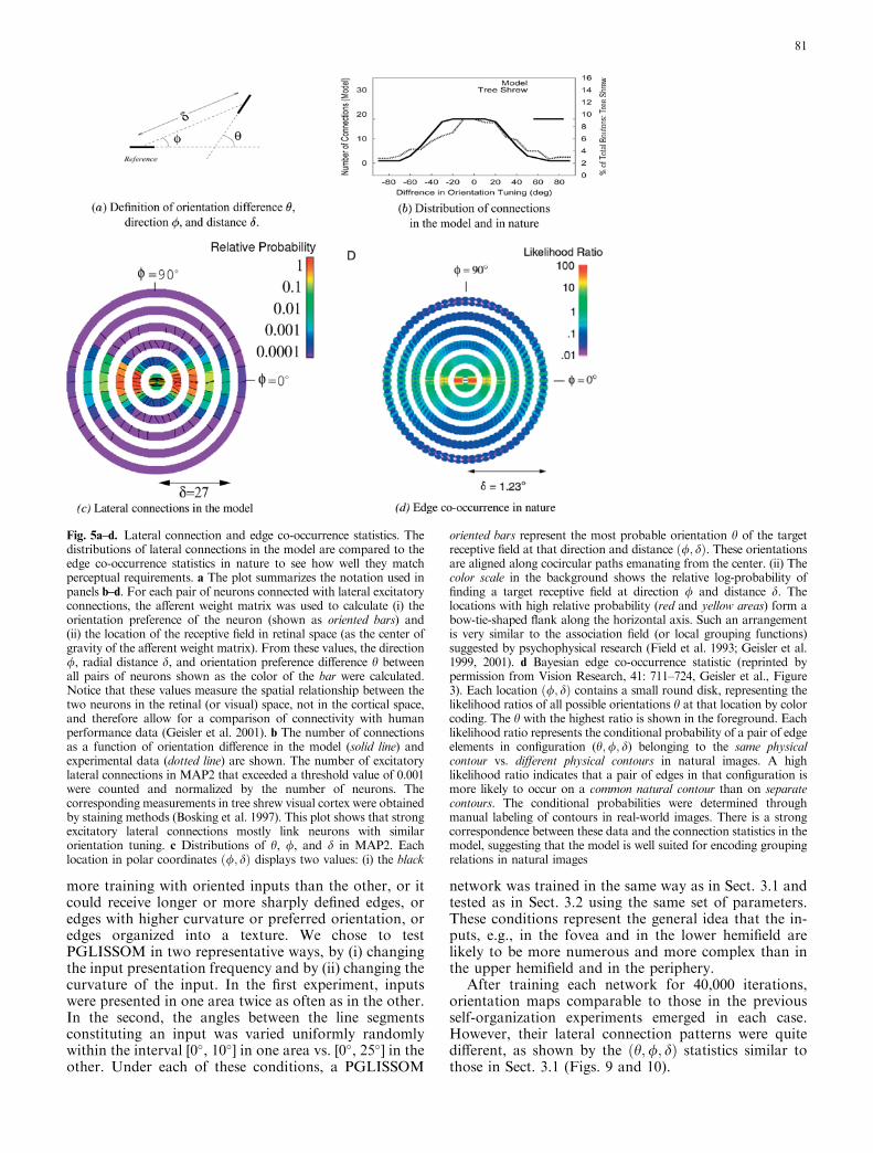
To quantify the grouping rules implemented by thelateral excitatory connections, their distributions in finalMAP2 were measured in detail (Fig. 5). Since thesedistributions are obtained from the receptive fields of theneurons, they describe the functional connectivity of theneurons in the retinal (i.e., visual) space rather thansimple cortical wiring statistics. The results confirm that(i) the lateral connections more often connect neuronswith similar orientation tuning (Fig. 5b) and (ii) con-nections go to target neurons with receptive fieldsaligned along the preferred orientation of the sourceneuron, with a small flank (Fig. 5c). In other words,neurons whose receptive fields fall on a smooth (cocir-cular) contour are most likely to be connected withstrong lateral excitatory connections in MAP2.

Interestingly, these connection statistics are verysimilar to the edge co-occurrence statistics in naturalimages (Geisler et al. 2001) (Fig. 5d). Combined withtransitive grouping rules, such edge co-occurrence sta-tistics can accurately predict human contour integrationperformance (Geisler et al. 1999, 2001). Therefore, weexpect the model to perform like humans as well. If thisprediction is confirmed, it lends computational supportto the idea that self-organized lateral connectivity in V1underlies contour integration performance in humans.

3.2 Contour integration

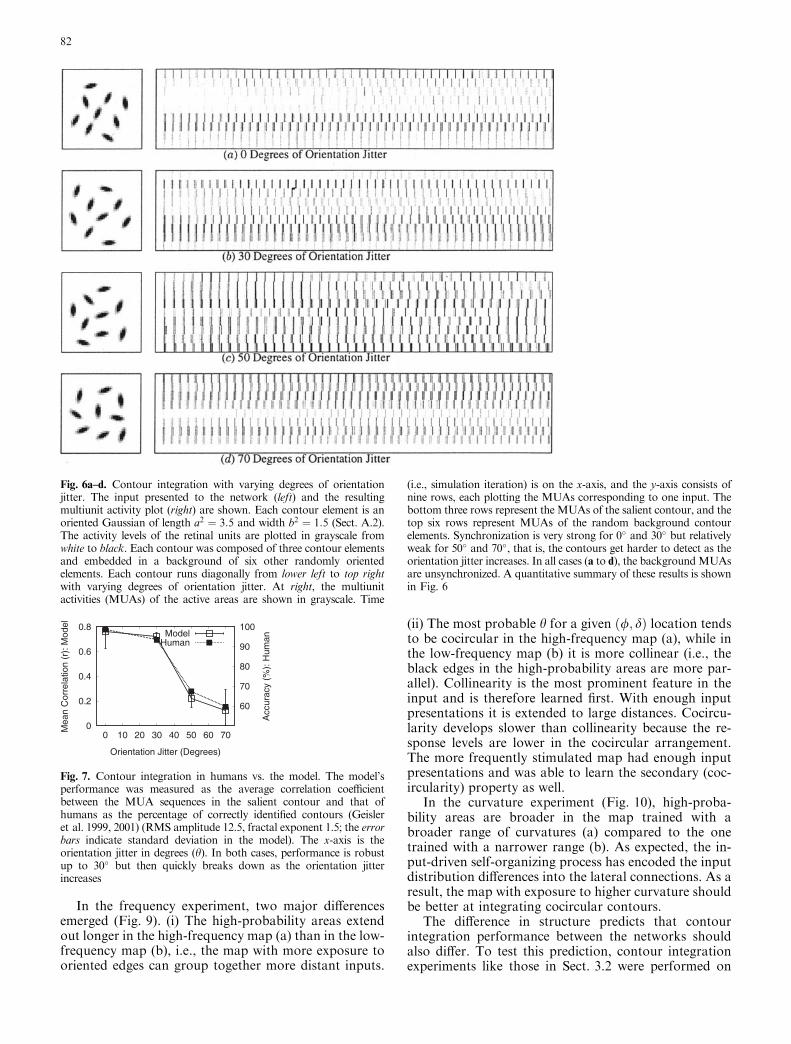
Psychological experiments by Field et al.(1993) andGeisler et al. (1999, 2001) have shown that contourintegration accuracy is maximal when orientation jitterin the physical contour is 0�, and the accuracy decreasesas a function of increasing orientation jitter. The lateralconnection statistics in the previous section are consis-tent with such behavior, but does the model actuallyperform that way? To answer this question, we ranseveral contour integration experiments with varyingdegrees of orientation jitter (Fig. 6).

To measure the performance of the model, for eachinput bar, the number of spikes generated by the area ofthe cortex that responded to the bar was counted at eachtime step. This quantity is called the multiunit activity ofthe response, or MUA, and it can be used to identifywhich area of the cortex is active at each time step. Todetermine the degree of synchronization between twoareas, the linear correlation coefficient r between theirMUA sequences was calculated as follows:

r ¼P

iðxi � �xÞðyi � �yÞffiffiffiffiffiffiffiffiffiffiffiffiffiffiffiffiffiffiffiffiffiffiffiffiPiðxi � �xÞ2

q ffiffiffiffiffiffiffiffiffiffiffiffiffiffiffiffiffiffiffiffiffiffiffiffiPiðyi � �yÞ2

q ; ð11Þ

where xi and yi, i ¼ 1; . . . ;N are the MUA values at timei for the two areas representing the two different objectsin the scene, and �x and �y are the mean of each sequence.

Fig. 3a,b. Orientation preferences in MAP1 and MAP2. The orien-tation preference at each location on the cortex is coded in color,according to the color key in the middle. The orientation preference ofeach neuron was calculated by taking a dot product of its afferentweight matrix and six different elongated Gaussians: the preferencewas the vector sum of six polar vectors, each consisting of the angle ofone Gaussian and its dot product (Bednar 1997; Blasdel 1992). Thesame organization of orientation preferences developed in both maps.The global and local features such as pinwheel centers and fractures ineach map closely match those found in the visual cortex

79

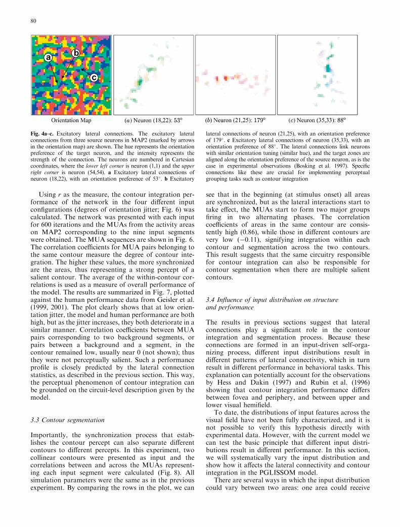
Using r as the measure, the contour integration per-formance of the network in the four different inputconfigurations (degrees of orientation jitter; Fig. 6) wascalculated. The network was presented with each inputfor 600 iterations and the MUAs from the activity areason MAP2 corresponding to the nine input segmentswere obtained. The MUA sequences are shown in Fig. 6.The correlation coefficients for MUA pairs belonging tothe same contour measure the degree of contour inte-gration. The higher these values, the more synchronizedare the areas, thus representing a strong percept of asalient contour. The average of the within-contour cor-relations is used as a measure of overall performance ofthe model. The results are summarized in Fig. 7, plottedagainst the human performance data from Geisler et al.(1999, 2001). The plot clearly shows that at low orien-tation jitter, the model and human performance are bothhigh, but as the jitter increases, they both deteriorate in asimilar manner. Correlation coefficients between MUApairs corresponding to two background segments, orpairs between a background and a segment, in thecontour remained low, usually near 0 (not shown); thusthey were not perceptually salient. Such a performanceprofile is closely predicted by the lateral connectionstatistics, as described in the previous section. This way,the perceptual phenomenon of contour integration canbe grounded on the circuit-level description given by themodel.

3.3 Contour segmentation

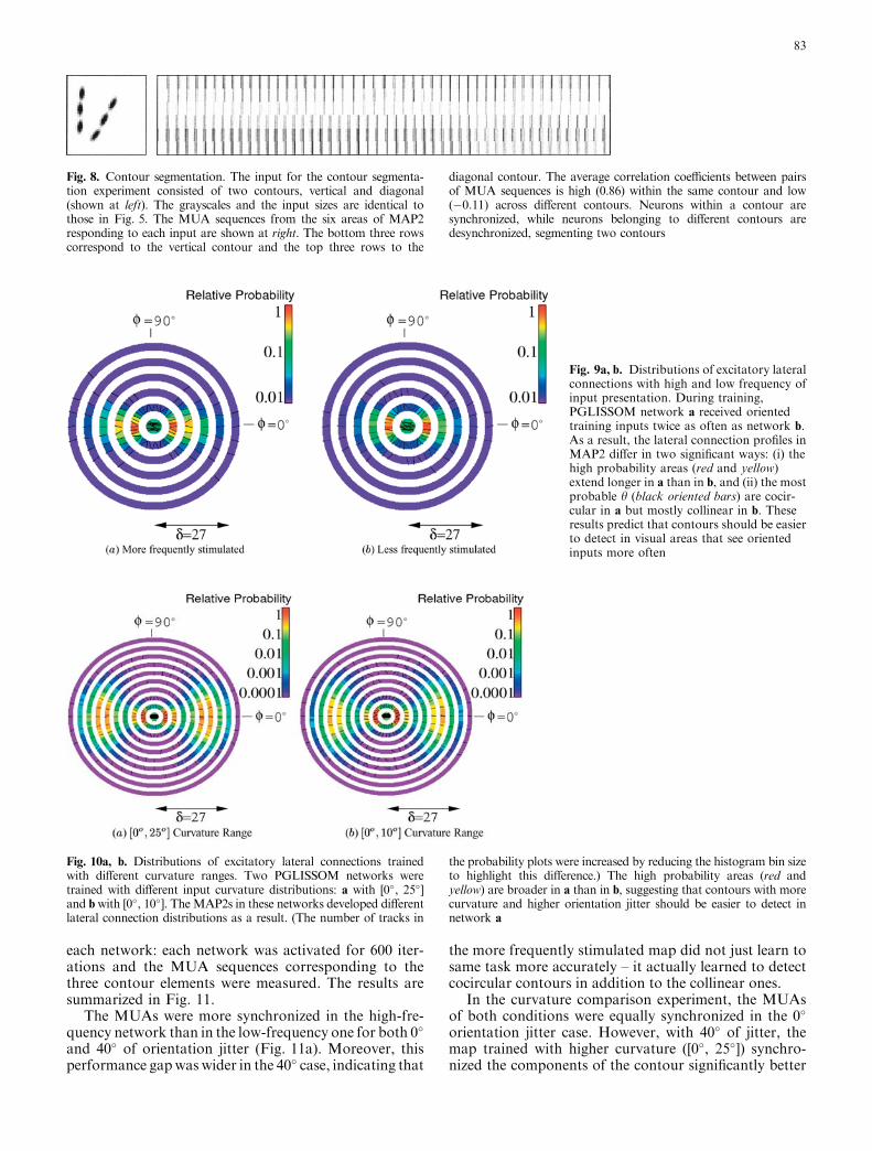
Importantly, the synchronization process that estab-lishes the contour percept can also separate differentcontours to different percepts. In this experiment, twocollinear contours were presented as input and thecorrelations between and across the MUAs represent-ing each input segment were calculated (Fig. 8). Allsimulation parameters were the same as in the previousexperiment. By comparing the rows in the plot, we can

see that in the beginning (at stimulus onset) all areasare synchronized, but as the lateral interactions start totake effect, the MUAs start to form two major groupsfiring in two alternating phases. The correlationcoefficients of areas in the same contour are consis-tently high (0.86), while those in different contours arevery low (�0:11), signifying integration within eachcontour and segmentation across the two contours.This result suggests that the same circuitry responsiblefor contour integration can also be responsible forcontour segmentation when there are multiple salientcontours.

3.4 Influence of input distribution on structureand performance

The results in previous sections suggest that lateralconnections play a significant role in the contourintegration and segmentation process. Because theseconnections are formed in an input-driven self-orga-nizing process, different input distributions result indifferent patterns of lateral connectivity, which in turnresult in different performance in behavioral tasks. Thisexplanation can potentially account for the observationsby Hess and Dakin (1997) and Rubin et al. (1996)showing that contour integration performance differsbetween fovea and periphery, and between upper andlower visual hemifield.

To date, the distributions of input features across thevisual field have not been fully characterized, and it isnot possible to verify this hypothesis directly withexperimental data. However, with the current model wecan test the basic principle that different input distri-butions result in different performance. In this section,we will systematically vary the input distribution andshow how it affects the lateral connectivity and contourintegration in the PGLISSOM model.

There are several ways in which the input distributioncould vary between two areas: one area could receive

Fig. 4a–c. Excitatory lateral connections. The excitatory lateralconnections from three source neurons in MAP2 (marked by arrowsin the orientation map) are shown. The hue represents the orientationpreference of the target neuron, and the intensity represents thestrength of the connection. The neurons are numbered in Cartesiancoordinates, where the lower left corner is neuron (1,1) and the upperright corner is neuron (54,54). a Excitatory lateral connections ofneuron (18,22), with an orientation preference of 53�. b Excitatory

lateral connections of neuron (21,25), with an orientation preferenceof 179�. c Excitatory lateral connections of neuron (35,33), with anorientation preference of 88�. The lateral connections link neuronswith similar orientation tuning (similar hue), and the target zones arealigned along the orientation preference of the source neuron, as is thecase in experimental observations (Bosking et al. 1997). Specificconnections like these are crucial for implementing perceptualgrouping tasks such as contour integration

80

more training with oriented inputs than the other, or itcould receive longer or more sharply defined edges, oredges with higher curvature or preferred orientation, oredges organized into a texture. We chose to testPGLISSOM in two representative ways, by (i) changingthe input presentation frequency and by (ii) changing thecurvature of the input. In the first experiment, inputswere presented in one area twice as often as in the other.In the second, the angles between the line segmentsconstituting an input was varied uniformly randomlywithin the interval [0�, 10�] in one area vs. [0�, 25�] in theother. Under each of these conditions, a PGLISSOM

network was trained in the same way as in Sect. 3.1 andtested as in Sect. 3.2 using the same set of parameters.These conditions represent the general idea that the in-puts, e.g., in the fovea and in the lower hemifield arelikely to be more numerous and more complex than inthe upper hemifield and in the periphery.

After training each network for 40,000 iterations,orientation maps comparable to those in the previousself-organization experiments emerged in each case.However, their lateral connection patterns were quitedifferent, as shown by the ðh;/; dÞ statistics similar tothose in Sect. 3.1 (Figs. 9 and 10).

Fig. 5a–d. Lateral connection and edge co-occurrence statistics. Thedistributions of lateral connections in the model are compared to theedge co-occurrence statistics in nature to see how well they matchperceptual requirements. a The plot summarizes the notation used inpanels b–d. For each pair of neurons connected with lateral excitatoryconnections, the afferent weight matrix was used to calculate (i) theorientation preference of the neuron (shown as oriented bars) and(ii) the location of the receptive field in retinal space (as the center ofgravity of the afferent weight matrix). From these values, the direction/, radial distance d, and orientation preference difference h betweenall pairs of neurons shown as the color of the bar were calculated.Notice that these values measure the spatial relationship between thetwo neurons in the retinal (or visual) space, not in the cortical space,and therefore allow for a comparison of connectivity with humanperformance data (Geisler et al. 2001). b The number of connectionsas a function of orientation difference in the model (solid line) andexperimental data (dotted line) are shown. The number of excitatorylateral connections in MAP2 that exceeded a threshold value of 0.001were counted and normalized by the number of neurons. Thecorresponding measurements in tree shrew visual cortex were obtainedby staining methods (Bosking et al. 1997). This plot shows that strongexcitatory lateral connections mostly link neurons with similarorientation tuning. c Distributions of h, /, and d in MAP2. Eachlocation in polar coordinates ð/; dÞ displays two values: (i) the black

oriented bars represent the most probable orientation h of the targetreceptive field at that direction and distance ð/; dÞ. These orientationsare aligned along cocircular paths emanating from the center. (ii) Thecolor scale in the background shows the relative log-probability offinding a target receptive field at direction / and distance d. Thelocations with high relative probability (red and yellow areas) form abow-tie-shaped flank along the horizontal axis. Such an arrangementis very similar to the association field (or local grouping functions)suggested by psychophysical research (Field et al. 1993; Geisler et al.1999, 2001). d Bayesian edge co-occurrence statistic (reprinted bypermission from Vision Research, 41: 711–724, Geisler et al., Figure3). Each location ð/; dÞ contains a small round disk, representing thelikelihood ratios of all possible orientations h at that location by colorcoding. The h with the highest ratio is shown in the foreground. Eachlikelihood ratio represents the conditional probability of a pair of edgeelements in configuration (h;/; d) belonging to the same physicalcontour vs. different physical contours in natural images. A highlikelihood ratio indicates that a pair of edges in that configuration ismore likely to occur on a common natural contour than on separatecontours. The conditional probabilities were determined throughmanual labeling of contours in real-world images. There is a strongcorrespondence between these data and the connection statistics in themodel, suggesting that the model is well suited for encoding groupingrelations in natural images

81

In the frequency experiment, two major differencesemerged (Fig. 9). (i) The high-probability areas extendout longer in the high-frequency map (a) than in the low-frequency map (b), i.e., the map with more exposure tooriented edges can group together more distant inputs.

(ii) The most probable h for a given ð/; dÞ location tendsto be cocircular in the high-frequency map (a), while inthe low-frequency map (b) it is more collinear (i.e., theblack edges in the high-probability areas are more par-allel). Collinearity is the most prominent feature in theinput and is therefore learned first. With enough inputpresentations it is extended to large distances. Cocircu-larity develops slower than collinearity because the re-sponse levels are lower in the cocircular arrangement.The more frequently stimulated map had enough inputpresentations and was able to learn the secondary (coc-ircularity) property as well.

In the curvature experiment (Fig. 10), high-proba-bility areas are broader in the map trained with abroader range of curvatures (a) compared to the onetrained with a narrower range (b). As expected, the in-put-driven self-organizing process has encoded the inputdistribution differences into the lateral connections. As aresult, the map with exposure to higher curvature shouldbe better at integrating cocircular contours.

The difference in structure predicts that contourintegration performance between the networks shouldalso differ. To test this prediction, contour integrationexperiments like those in Sect. 3.2 were performed on

Fig. 7. Contour integration in humans vs. the model. The model’sperformance was measured as the average correlation coefficientbetween the MUA sequences in the salient contour and that ofhumans as the percentage of correctly identified contours (Geisleret al. 1999, 2001) (RMS amplitude 12.5, fractal exponent 1.5; the errorbars indicate standard deviation in the model). The x-axis is theorientation jitter in degrees (h). In both cases, performance is robustup to 30� but then quickly breaks down as the orientation jitterincreases

Fig. 6a–d. Contour integration with varying degrees of orientationjitter. The input presented to the network (left) and the resultingmultiunit activity plot (right) are shown. Each contour element is anoriented Gaussian of length a2 ¼ 3:5 and width b2 ¼ 1:5 (Sect. A.2).The activity levels of the retinal units are plotted in grayscale fromwhite to black. Each contour was composed of three contour elementsand embedded in a background of six other randomly orientedelements. Each contour runs diagonally from lower left to top rightwith varying degrees of orientation jitter. At right, the multiunitactivities (MUAs) of the active areas are shown in grayscale. Time

(i.e., simulation iteration) is on the x-axis, and the y-axis consists ofnine rows, each plotting the MUAs corresponding to one input. Thebottom three rows represent the MUAs of the salient contour, and thetop six rows represent MUAs of the random background contourelements. Synchronization is very strong for 0� and 30� but relativelyweak for 50� and 70�, that is, the contours get harder to detect as theorientation jitter increases. In all cases (a to d), the backgroundMUAsare unsynchronized. A quantitative summary of these results is shownin Fig. 6

82

each network: each network was activated for 600 iter-ations and the MUA sequences corresponding to thethree contour elements were measured. The results aresummarized in Fig. 11.

The MUAs were more synchronized in the high-fre-quency network than in the low-frequency one for both 0�

and 40� of orientation jitter (Fig. 11a). Moreover, thisperformance gapwas wider in the 40� case, indicating that

the more frequently stimulated map did not just learn tosame task more accurately – it actually learned to detectcocircular contours in addition to the collinear ones.

In the curvature comparison experiment, the MUAsof both conditions were equally synchronized in the 0�

orientation jitter case. However, with 40� of jitter, themap trained with higher curvature ([0�, 25�]) synchro-nized the components of the contour significantly better

Fig. 9a, b. Distributions of excitatory lateralconnections with high and low frequency ofinput presentation. During training,PGLISSOM network a received orientedtraining inputs twice as often as network b.As a result, the lateral connection profiles inMAP2 differ in two significant ways: (i) thehigh probability areas (red and yellow)extend longer in a than in b, and (ii) the mostprobable h (black oriented bars) are cocir-cular in a but mostly collinear in b. Theseresults predict that contours should be easierto detect in visual areas that see orientedinputs more often

Fig. 10a, b. Distributions of excitatory lateral connections trainedwith different curvature ranges. Two PGLISSOM networks weretrained with different input curvature distributions: a with [0�, 25�]and bwith [0�, 10�]. TheMAP2s in these networks developed differentlateral connection distributions as a result. (The number of tracks in

the probability plots were increased by reducing the histogram bin sizeto highlight this difference.) The high probability areas (red andyellow) are broader in a than in b, suggesting that contours with morecurvature and higher orientation jitter should be easier to detect innetwork a

Fig. 8. Contour segmentation. The input for the contour segmenta-tion experiment consisted of two contours, vertical and diagonal(shown at left). The grayscales and the input sizes are identical tothose in Fig. 5. The MUA sequences from the six areas of MAP2responding to each input are shown at right. The bottom three rowscorrespond to the vertical contour and the top three rows to the

diagonal contour. The average correlation coefficients between pairsof MUA sequences is high (0.86) within the same contour and low(�0:11) across different contours. Neurons within a contour aresynchronized, while neurons belonging to different contours aredesynchronized, segmenting two contours

83

(Fig. 11b). The more cocircular lateral connections al-lowed this map to synchronize line segments that wereless perfectly aligned.

These results show that if the input distribution variesacross different areas of the visual field, the input-drivenself-organization process will shape the connectionsaccordingly, and such structural differences will lead todifferent performance in contour integration. This is animportant prediction of the model that in the future canbe tested with input variation in natural visual input.Such studies can eventually lead to a computationalexplanation of why visual performance differs across thevisual field, and perhaps to some extent even in differentspecies.

4 Discussion

Our results show that the specific lateral connectivitynecessary for contour integration can be due to input-driven self-organization. The same self-organizationmechanism was previously shown to be potentiallyresponsible for orientation, ocular dominance, andfrequency columns and patchy connections betweenthem, for repair after cortical and retinal damage, andfor tilt aftereffects (Miikkulainen et al. 1997), providinga unified explanation of several different phenomena inthe visual cortex. The main new idea advanced in thispaper is that long-range excitatory lateral connectionscan also self-organize into highly specific patterns thatserve a perceptual grouping function.

The connection patterns that emerge in the modelclosely approximate those found in neurophysiologicalexperiments (Bosking et al. 1997; Fitzpatrick et al. 1994)and are very similar to the local contour grouping sta-tistics found in natural images (Geisler et al. 1999, 2001).They also generally agree with connection patternshypothesized in hand-coded computational models (Li1998; Ross et al. 2000; Yen and Finkel 1997, 1998). Wealso demonstrated that synchronized firing of neuronalpopulations can represent the percept of contour verywell by comparing correlations to human contour inte-gration accuracy with varying degrees of orientationjitter (Field et al. 1993; Geisler et al. 1999; Geisler et al.2001).

The input patterns studied in this paper are decidedlysimple for two reasons: (i) they make it is possible tocharacterize and measure model behavior clearly, with-out confounding factors, and (ii) more complex patternswould require larger networks, which are computation-ally too expensive to simulate at the moment. Forexample, the current self-organization simulationsrequired about 200 MB of memory and took about 20 hon a 1.7-GHz Pentium PC. To represent more complexinputs, the number of rows and columns would have tobe scaled up by a factor of four, resulting in a simulationwith over 40 GB of memory and a training time of over4800 h. However, there is good reason to believe that themodel will scale up well: it is based on regular patterns ofconnectivity that can be duplicated horizontally, result-ing in a larger-scale model with similar behavior. In a

parallel line of research, we have developed methods forsuch incremental scaling of self-organizing firing-ratemodels (Bednar et al. 2002); applying these methods tothe contour integration task is a most interesting direc-tion of future work. The temporal behavior of the modelshould also scale up well. Campbell et al. (1999) recentlyshowed that time to synchronization in locally con-nected integrate-and-fire neurons is logarithmicallyproportional to the network size. Since the dynamicthreshold neuron used in the current model is equivalentto integrate-and-fire neurons, we expect our model toshow similar, manageable temporal scaling behavior asthe network size is increased. In the near future, suffi-cient computational power might exist to train themodel with natural images. Based on analogous resultswith firing-rate models (Bednar et al. 2002), we expectthe results with more complex images to be similar tothose of the current model.

Whether or not contour integration in the modeloccurs depends on whether the appropriate lateral con-nections exist. Integration is possible only if focused(i.e., patchy) lateral connections link neurons with sim-ilar orientation preferences. Even though the integrationand adaptation mechanisms might be the samethroughout the cortex, if the input to the different areasdiffers during development, different contour integrationperformance results. The model therefore suggests whythe performance, e.g., in the upper vs. lower hemifield(or in fovea vs. periphery) might differ: if the upper vi-sual field does not receive sufficiently dense visual inputduring development, its lateral connections remain dif-fuse, resulting in weaker integration. We plan to test thishypothesis in the future with a model that also takes intoaccount the structural differences in these areas, such asdifferent receptor densities. In this way, the observeddifferences in contour integration performance canpossibly be explained as an effect of input-driven self-organization.

Statistics of images projected on the retina indeedsupport the idea that input distributions may differamong different visual areas. Reinagel and Zador (1999)showed that human gaze most often falls upon areaswith high contrast and low pixel correlation. As a result,sharper images may project more often on the foveathan the periphery, allowing more specific connectionsto form. A similar method can be used to find out ifthere is a difference in statistical distribution of imagefeatures in the lower vs. upper hemisphere. This seemslikely, based on the observation that primates mostlymanipulate objects in their lower hemifield (Previc1990). Such statistical differences together with Hebbianself-organization would then result in different contourintegration capability in different visual areas, as wasdemonstrated in Sect. 3.4.

A competing hypothesis would be that the differencesbetween hemifields (as well as those between fovea andperiphery) are genetically determined. One way of dis-tinguishing between these hypotheses would be to rearan animal with eye glasses that flip the input to the upperand lower hemifield. After the critical period, the ani-mal’s performance on contour detection task could be

84

measured and the connectivity patterns formed in theupper and lower hemifield compared to normally rearedcontrol animals. With genetic determination thereshould be no noticeable difference, whereas PGLISSOMpredicts that high connectivity and good integrationwould occur in the upper hemifield, instead of the lowerhemifield as in control animals.

The fact that even simple patterns such as straightGaussian bars shape the circuitry for contour integrationis an interesting result. It supports a previous proposal byBednar and Miikkulainen (1998, 2000a) that simpleinternally generated patterns in the developing nervoussystem may pretrain the cortex before birth, explainingwhy a certain degree of organization and functionalityalready exists in a newborn cortex. However, since thePGLISSOM model was trained with straight Gaussianbars, one would expect only collinear properties toemerge in the connection profile, instead of the cocircularpatterns actually observed (Fig. 5). Such an unexpectedresult follows fromHebbian learning on graded responses(Fig. 12). Neurons coactivate even if their receptive fieldsare not perfectly aligned, allowing cocircular connectionsto develop along with the collinear ones. Such gradedtraining in general matches the regularities in the visualenvironment, forming a robust starting point for learningmore refined regularities in the visual input.

As we have seen in this paper, connection statistics,feature co-occurrence statistics, and performance arevery closely related. It may be possible to measure co-occurrence statistics of visual features other than ori-entation as well, and such statistics could be used toderive hypotheses about the functional connectivity ofvisual cortical areas. Thus perceptual grouping rulesemployed by the brain can be systematically investigatedby examining the statistical structure in natural scenes.

5 Conclusion

This paper shows how the specific connection patternsthat may facilitate contour integration and segmentation

in the visual cortex can be due to the same generalprocess of input-driven self-organization as in manyother cortical structures. The contour integration per-formance measured by the degree of synchronization inthe model matches human performance data very well,lending further support to the idea that segmentationand binding could be due to synchronized firing ofneuronal groups. The model also suggests that differ-ently distributed input presentations and the resultinglateral connections may be the cause of the differentdegrees of contour integration observed in the differentvisual areas. It should be possible to account for otherlow-level Gestalt phenomena with similar computationalprinciples.

Acknowledgement Thanks to Wilson Geisler for the human dataand to James Bednar for insightful comments on an earlier versionof the manuscript. We would also like to thank the anonymousreviewer for helpful comments on Sect. 3.4. This research wassupported in part by National Science Foundation grant IRI-9811478, National Institutes of Mental Health (Human BrainProject) grant 1R01-MH66991, and Texas Higher EducationCoordinating Board grant 000512-0217-2001.

A Appendix: Simulation setup

This section describes the simulation setup in detail foraccurate replication of the results presented in thispaper. The code and simulation configuration files canbe found on the World Wide Web at http://www.cs.tamu.edu/faculty/choe.

A.1 Network

While MAP1 consisted of 136� 136 neurons, MAP2was reduced to 54� 54 to save simulation timeand memory. The intracolumnar connections betweenMAP1 and MAP2 were proportional to scale, so thatthe relative locations of corresponding neurons in thetwo maps were the same. However, different parameter

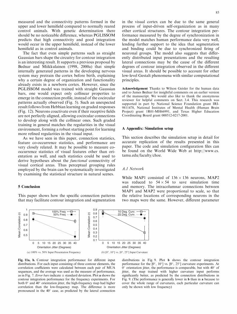
Fig. 11a, b. Contour integration performance for different inputdistributions. For each input consisting of three contour elements, thecorrelation coefficients were calculated between each pair of MUAsequences, and the average was used as the measure of performance,as in Fig. 7. Error bars indicate� standard deviation. Plot a shows thecontour integration performance for the frequency experiments. Forboth 0� and 40� orientation jitter, the high-frequency map had highercorrelation than the low-frequency map. The difference is morepronounced in the 40� case, as predicted by the lateral connection

distributions in Fig. 9. Plot b shows the contour integrationperformance for the [0�, 10�] vs. [0�, 25�] curvature experiments. At0� orientation jitter, the performance is comparable, but with 40� ofjitter, the map trained with higher curvature input performssignificantly better, as predicted by the connection distributions inFig. 9. (The performance is generally lower in b than in a because tocover the whole range of curvatures, each particular curvature canonly be shown with low frequency)

85

values were required for the two maps, corresponding totheir different sizes. Excitatory lateral connections inMAP1 had an initial radius of 7 and gradually reducedto 3, and inhibitory lateral connections had a fixedradius of 10. Initially, large areas have correlated activityso that global order can be formed, and later on thereduced lateral excitatory connections help fine-tune thelocal order in the map (Kohonen 1982, 1989, 1993;Sirosh and Miikkulainen 1997). In MAP2, excitatorylateral connections had a radius of 40 and 54 inhibitoryconnections. Afferent connections to the retina had aradius of 6 in both maps and intracolumnar connectionsa radius of 2 in both maps. The retina consisted of46� 46 receptors, except for Sect. 3.4 where it was72� 72 to have sufficiently large lower and upperhemifields for the experiments. As long as the relativesizes of the map, the retina, and the lateral connectionradii are similar to these values, the maps self-organizewell (see Bednar et al. 2002 for precise equations thatallow scaling maps to different sizes).

A.2 Self-organization

This section describes the simulation setup used inSects. 3.1 and 3.4. The input in the training experimentconsisted of straight oriented Gaussians:

nr1;r2 ¼ expð� ððr1 � xÞ cosð/Þ � ðr2 � yÞ sinð/ÞÞ2

a2

� ððr1 � xÞ sinð/Þ þ ðr2 � yÞ cosð/ÞÞ2

b2Þ ; ð12Þ

where nr1;r2 is the desired activity of the retinal neuron atlocation (r1; r2), a2 and b2 specify the length along themajor and minor axes of the Gaussian, and / specifiesits orientation. These axis lengths were a2 ¼ 15:0 andb2 ¼ 0:6 for the first 1,000 iterations, and they wereincreased to 45.0 and 0.45 thereafter, except for Sect. 4where the axis lengths were a2 ¼ 15:0 and b2 ¼ 1:3 at thebeginning and increased to 50.0 and 0.8 by iteration10,000, to compensate for the enlarged retina size. Allweights were initialized with uniform random numberswithin ½0::1�. The relative contributions of afferent,lateral excitatory, lateral inhibitory, and intracolumnarconnections were ca ¼ 1:1, ce ¼ 0:8, ci ¼ 0:9, andcc ¼ 0:5 for MAP1 and ca ¼ 1:1, ce ¼ 0:2, ci ¼ 2:5, and

cc ¼ 0:9 for MAP2. The learning rates of afferent, lateralexcitatory, lateral inhibitory, and intra-columnar con-nections were aa ¼ 0:012, ae ¼ 0:008, ai ¼ 0:008, andac ¼ 0:012 for MAP1 and aa ¼ 0:012, ae ¼ 0:008,ai ¼ 0:0, and ac ¼ 0:012, for MAP2. At 5,000 iterations,aa and ac in both maps were decreased to 0.008 so thatthe global order in the map could start stabilizing. Initialbase threshold hbase for both maps was 0.05. At thebeginning of each settling iteration, the hbase wasadjusted to 50% of maxi;jðri;jðtÞÞ so that the networkwould not become too active or totally silent. Later, thepercentage was increased to 57.5% at 15,000 iterationsfor MAP1 and 65% at 5,000 for MAP2. Whileorganized maps can be obtained without such parameteradaptation, using them generally leads to better results.Interestingly, biological evidence also supports suchadaptation processes during learning, including boththreshold adaptation (Azouz and Gray 2000; Prince andHuguenard 1988) and synaptic plasticity (Caleo andMaffei 2002).

The synaptic decay rates were different for differenttypes of connections. Previous sum was decayed by e�k,where k ¼ 3:0; 0:5; and 1.0 for lateral excitatory, inhib-itory, and intracolumnar connections, respectively, forboth maps. The decay rate in the spike generator’sinhibitory feedback krel ¼ 0:5 in both maps. The relativecontribution of the inhibitory feedback in dynamicthreshold calculation was s ¼ 0:4 in both maps. Thethreshold and ceiling of the linear approximation of thesigmoid function gð�Þ were d ¼ 0:01 and b ¼ 1:3 in bothmaps. For the average spiking rate of neurons, a runningaverage with the rate savg ¼ 0:92 was calculated.

A.3 Contour integration and segmentation

This section describes the setup for contour integrationexperiments in Sects. 3.2, 3.3, and 3.4. The input to thenetwork consisted of oriented Gaussians of lengtha2 ¼ 3:5 and width b2 ¼ 1:5 (Eq. 12). Examples areshown in Fig. 6. For the training, a long Gaussian wasnecessary, but for the contour integration experiments,they were short enough to fit into a single receptive field(afferent connection radius = 6).

The network configuration and parameters were thesame as in Sect. A.2, except for the following changes:The lateral excitatory connections in MAP2 with weightsless than 0.001 were deleted, modeling death of unusedconnections Katz and Callaway (1992), and ce in MAP2was increased to 0.8. In addition, the excitatory learningrate ae in MAP2 was set to 0.1. Although not strictlynecessary for grouping, this fast learning makes thepatchy connections more uniform and helps promotesynchrony among the connected regions; it does notaffect the patchy structure of the connections or theorganization of the map. Fast adaptation has been pro-posed to be useful in several forms (von der Malsburg1981; Crick 1984; Wang 1996), but it remains to be ver-ified in biological systems, and its role in smoothing theresponse constitutes a further prediction of the model. Tohelp desynchronization (segmentation) and model

Fig. 12a, b. Simultaneous activation of neurons. The plot shows tworepresentative cases of coactivation (i.e., when two neurons areactivated simultaneously), when a long (dashed line) input is presentedacross the two receptive fields. a Collinear arrangement: the tworeceptive fields (thick bars) are precisely aligned. If a long input ispresented along the same direction, the two neurons will respondmaximally, and the connection between them becomes stronger.b Cocircular arrangement: even though the two receptive fields areslightly misaligned, they are still weakly activated and their connectionis strengthened, although less so than in a

86

synaptic noise, MAP2 ci was increased to 5.0 and 4%noise was added. Previously, for self-organization, theabsolute refractory period (jabs) was set to 0. The firingrates of the neurons were high as a result and the simu-lation proceeded in a fast time scale. For the contourintegration experiments, a finer degree of temporal res-olution was necessary, so jabs was increased to 4.

References

Azouz R, Gray CM (2000) Dynamic spike threshold reveals amechanism for synaptic coincidence detection in cortical neu-rons in vivo. Proc Natl Acad Sci USA 97: 8110–8115

Bartsch AP, van Hemmen JL (2001) Combined Hebbian develop-ment of Geniculocortical and lateral connectivity in a model ofprimary visual cortex. Biol Cybern 84: 41–55

Bednar JA (1997) Tilt aftereffects in a self-organizing model of theprimary visual cortex. Master’s thesis, Department of Com-puter Sciences, University of Texas at Austin, Austin, TXTechnical Report AI97-259

Bednar JA (2002) Learning to see: genetic and environmentalinfluences on visual development. PhD thesis, Department ofComputer Sciences, University of Texas at Austin, Austin, TX

Bednar JA, Kelkar A, Miikkulainen R (2002) Modeling largecortical networks with growing self-organizing maps. In: BowerJM (ed) Computational neuroscience: trends in research.Elsevier, New York (in press)

Bednar JA, Miikkulainen R (1998) Pattern-generator-driven devel-opment in self-organizing models. In: Bower JM (ed) Compu-tational neuroscience: trends in research. Plenum,NewYork, pp317–323

Bednar JA, Miikkulainen R (2000a) Self-organization of innate facepreferences: could genetics be expressed through learning? In:Proceedings of the 17th national conference on artificial intelli-gence (AAAI-2000), Austin, TX, July–August 2000. MIT Press,Cambridge, MA, pp 117–122

Bednar JA, Miikkulainen R (2000b) Tilt aftereffects in a self-organizing model of the primary visual cortex. Neural Comput12 (7): 1721–1740

Blasdel GG (1992) Orientation selectivity, preference, and conti-nuity in monkey striate cortex. J Neurosci 12: 3139–3161

Blasdel GG, Salama G (1986) Voltage-sensitive dyes reveal amodular organization in monkey striate cortex. Nature 321:579–585

Bosking WH, Zhang Y, Schofield B, Fitzpatrick D (1997) Orien-tation selectivity and the arrangement of horizontal connec-tions in tree shrew striate cortex. J Neurosci 17 (6): 2112–2127

Burger T, Lang EW (1999) An incremental Hebbian learningmodel of the primary visual cortex with lateral plasticity andreal input patterns. Zeitschrift fu r Naturforschung C – J Biosci54: 128–140

Caleo M, Maffei L (2002) Neurotrophins and plasticity in thevisual cortex. Neuroscientist 8: 52–61

Campbell SR, Wang DL, Jayaprakash C (1999) Synchrony anddesynchrony in integrate-and-fire oscillators. Neural Comput11: 1595–1619

Choe Y (2001) Perceptual grouping in a self-organizing map ofspiking neurons. PhD thesis, Department of Computer Sci-ences, University of Texas at Austin, Austin, TX. TechnicalReport AI01-292

Choe Y, Miikkulainen R (1998) Self-organization and segmenta-tion in a laterally connected orientation map of spiking neu-rons. Neurocomputing 21: 139–157

Crick F (1984) Function of the thalamic reticular complex: Thesearchlight hypothesis. Proc Natl Acad Sci USA 81: 4586–4950

Eckhorn R, Bauer R, Jordan W, Kruse M, Munk W, Reitboeck HJ(1988) Coherent oscillations: a mechanism of feature linking inthe visual cortex? Biol Cybern 60: 121–130

Eckhorn R, Reitboeck HJ, Arndt M, Dicke P (1990) Featurelinking via synchronization among distributed assemblies:Simulations of results from cat visual cortex. Neural Comput 2:293–307

Engel AK, Kreiter AK, Konig P, Singer W (1991) Synchronizationof oscillatory neuronal responses between striate and extras-triate visual cortical areas of the cat. Proc Natl Acad Sci USA88: 6048–6052

Field DJ, Hayes A, Hess RF (1993) Contour integration by thehuman visual system: evidence for a local association field.Vision Res 33: 173–193

Fitzpatrick D, Schofield BR, Strote J (1994) Spatial organizationand connections of iso-orientation domains in the tree shrewstriate cortex. Soc Neurosci Abstr 20: 837

Geisler WS, Thornton T, Gallogly DP, Perry JS (1999) Imagestructure models of texture and contour visibility. In: NATOworkshop on search and target acquisition, 1999

Geisler WS, Perry JS, Super BJ, Gallogly DP (2001) EdgeCo-occurrence in natural images predicts contour groupingperformance. Vision Res 41: 711–724

Gerstner W (1998) Spiking neurons. In: Maass W, Bishop CM(eds) Pulsed neural networks, chap 1. MIT Press, Cambridge,MA, pp 3–54

Gilbert CD, Wiesel TN (1990) The influence of contextual stimulion the orientation selectivity of cells in primary visual cortex ofthe cat. Vision Res 30 (11): 1689–1701

Goodhill GJ, Cimponeriu A (2000) Analysis of the elastic netmodel applied to the formation of ocular dominance and ori-entation columns. Network 11: 153–168

Gray CM, Konig P, Engel A, Singer W (1989) Oscillatory re-sponses in cat visual cortex exhibit inter-columnar synchroni-zation which reflects global stimulus properties. Nature 338:334–337

Gray CM (1999) The temporal correlation hypothesis of visualfeature integration: still alive and well. Neuron 24: 31–47

Gray CM, Singer W (1987) Stimulus specific neuronal oscillationsin the cat visual cortex: a cortical functional unit. Soc NeurosciAbstr 13: 404.3

Grinvald A, Lieke EE, Frostig RD, Hildesheim R (1994) Corticalpoint-spread function and long-range lateral interactions re-vealed by real-time optical imaging of macaque monkeyprimary visual cortex. J Neurosci 14: 2545–2568

Grossberg S, Grunewald A (1997) Cortical synchronization andperceptual framing. J Cogn Neurosci 9: 106–111

Grossberg S, Williamson JR (2001) A neural model of how hori-zontal and interlaminar connections of visual cortex developinto adult circuits that carry out perceptual grouping andlearning. Cereb Cortex 9: 878–895

Hata Y, Tsumoto T, Sato H, Hagihara K, Tamura H (1988)Inhibition contributes to orientation selectivity in the visualcortex of the cat. Nature 335: 815–817

Hess RF, Dakin SC (1997). Absence of contour linking inperipheral vision. Nature 390: 602–604

Hirsch JA, Gilbert CD (1991) Synaptic physiology of horizontalconnections in the cat’s visual cortex. J Neurosci 11: 1800–1809

Horn D, Opher I (1998) Collective excitation phenomenon and theirapplications. In: Maass W, Bishop CM (eds) Pulsed neural net-works, chap 11. MIT Press, Cambridge, MA, pp 297–320

Kammen DM, Holmes PJ, Koch C (1989) Origin of oscillations invisual cortex: feedback versus local coupling. In: Cotterill RMJ(ed) Models of brain functions. Cambridge University Press,Cambridge, UK, pp 273–284

Katz LC, Callaway EM (1992) Development of local circuits inmammalian visual cortex. Annu Rev Neurosci 15: 31–56

Kohonen T (1981) Automatic formation of topological maps ofpatterns in a self-organizing system. In: Proceedings of the 2ndScandinavian conference on image analysis, Espoo, Finland,June 1981, pp 214–220

Kohonen T (1982) Self-organized formation of topologically cor-rect feature maps. Biol Cybern 43: 59–69

87

Kohonen T (1989) Self-organization and associative memory, 3rdedn. Springer, Berlin Heidelberg New York

KohonenT (1993) Physiological interpretation of the self-organizingmap algorithm. Neural Netw 6: 895–905

Kohonen T (1995) Self-organizing maps. Springer, Berlin Heidel-berg New York

Li Z (1998) A neural model of contour integration in the primaryvisual cortex. Neural Comput 10: 903–940

Miikkulainen R, Bednar JA, Choe Y, Sirosh J (1997) Self-organi-zation, plasticity, and low-level visual phenomena in a laterallyconnectedmapmodel of the primary visual cortex. In:GoldstoneRL, Schyns PG, Medin DL (eds) Perceptual learning, vol 36 ofPsychology of learning and motivation. Academic, San Diego,CA, pp 257–308

Miller KD (1994) A model for the development of simple cellreceptive fields and the ordered arrangement of orientationcolumns through activity-dependent competition betweenON- and OFF-center inputs. J Neurosci 14: 409–441

Obermayer K, Ritter HJ, Schulten KJ (1990) A principle for theformation of the spatial structure of cortical feature maps. ProcNatl Acad Sci USA 87: 8345–8349

Pettet MW, McKee SP, Grzywacz NM (1998) Constraints on longrange interactions mediating contour detection. Vision Res 38:865–879

Previc FH (1990) Functional specialization in the lower and uppervisual fields in humans: Its ecological origins and neurophysi-ological implications. Behav Brain Sci 13: 519–575

Prince DA, Huguenard JR (1988) Functional properties of neo-cortical neurons. In: Rakic P, Singer W (eds) Neurobiology ofneocortex. Wiley, New York, pp 153–176

Reinagel P, Zador AM (1999) Natural scene statistics at the centerof gaze. Netw Comput Neural Sys 10: 1–10

Reitboeck H, Stoecker M, Hahn C (1993) Object separation indynamic neural networks. In: Proceedings of the IEEE inter-national conference on neural networks, San Francisco, CA, 2:638–641. IEEE, Piscataway, NJ

Ross WD, Grossberg S, Mingolla E (2000) Visual cortical mech-anisms of perceptual grouping: interacting layers, networks,columns, and maps. Neural Netw 13: 571–588

Rubin N, Nakayama K, Shapley R (1996) Enhanced perception ofillusory contours in the lower versus upper visual hemifields.Science 271: 651–653

Singer W (1999) Neuronal synchrony: a versatile code for thedefinition of relations? Neuron 24: 49–65

Singer W, Gray CM (1995) Visual feature integration and thetemporal correlation hypothesis. Annu Rev Neurosci 18: 555–586

Sirosh J (1995) A self-organizing neural network model of theprimary visual cortex. PhD thesis, Department of Computer

Sciences, University of Texas at Austin, Austin, TX. TechnicalReport AI95-237

Sirosh J, Miikkulainen R (1997) Topographic receptive fields andpatterned lateral interaction in a self-organizing model of theprimary visual cortex. Neural Comput 9: 577–594

Sirosh J, Miikkulainen R, Choe Y (eds) (1996) Lateral interactionsin the cortex: structure and function. The UTCS Neural Net-works Research Group, Austin, TX. Electronic book, ISBN 0-9647060-0-8, http://www.cs.utexas.edu/users/nn/web-pubs/htmlbook96

Swindale NV (1996) The development of topography in the visualcortex: a review of models. Netw Comput Neural Sys 7: 161–247

Terman D, Wang D (1995) Global competition and local cooper-ation in a network of neural oscillators. Physica D 81: 148–176

VanRullen R, Delorme A, Thorpe SJ (2001) Feed-forward contourintegration in primary visual cortex based on asynchronousspike propagation. Neurocomputing 38–40: 1003–1009

Von der Malsburg C (1973) Self-organization of orientation-sensitive cells in the striate cortex. Kybernetik 15: 85–100

Von der Malsburg C (1981) The correlation theory of brainfunction. Internal Report 81-2, Department of Neurobiology,Max-Planck-Institute for Biophysical Chemistry, Gottingen,Germany

Von der Malsburg C (1986) A neural cocktail-party processor. BiolCybern 54: 29–40

Von der Malsburg C (1987) Synaptic plasticity as basis of brainorganization. In: Changeux J-P, Konishi M (eds) The neuraland molecular bases of learning. Wiley, New York, pp 411–432

Von der Malsburg C, Buhmann J (1992) Sensory segmentationwith coupled neural oscillators. Biol Cybern 67: 233–242

Wang DL (1995) Emergent synchrony in locally coupled neuraloscillators. IEEE Trans Neural Netw 6: 941–948

Wang D (1996) Synchronous oscillations based on lateral connec-tions. In: Sirosh J, Miikkulainen R, Choe Y (eds) Lateralinteractions in the cortex: structure and function. UTCS NeuralNetworks Research Group, Austin, TX. Electronic book,ISBN 0-9647060-0-8, http://www.cs.utexas.edu/users/nn/web-pubs/htmlbook96

Wang D (2000) On connectedness: a solution based on oscillatorycorrelation. Neural Comput 12: 131–139

Weliky M, Kandler K, Fitzpatrick D, Katz LC (1995) Patterns ofexcitation and inhibition evoked by horizontal connections invisual cortex share a common relationship to orientationcolumns. Neuron 15: 541–552

Yen S-C, Finkel LH (1997) Identification of salient contours incluttered images. Comput Vision Patt Recog volume: 273–279

Yen S-C, Finkel L (1998) Extraction of perceptually salientcontours by striate cortical networks. Vision Res 38: 719–741

88