contractual pricing problems for retail distribution under …
TRANSCRIPT

CONTRACTUAL PRICING PROBLEMS FOR RETAIL DISTRIBUTION
UNDER DIFFERENT CHANNEL STRUCTURES
A Dissertation
by
SU ZHAO
Submitted to the Office of Graduate and Professional Studies ofTexas A&M University
in partial fulfillment of the requirements for the degree of
DOCTOR OF PHILOSOPHY
Chair of Committee, Sıla CetinkayaCo-Chair of Committee, Eylem TekinCommittee Members, Abhijit Deshmukh
Catherine YanHead of Department, Cesar O. Malave
December 2014
Major Subject: Industrial and System Engineering
Copyright 2014 Su Zhao

ABSTRACT
In many industries, including the retail industry, the profits of a supply chain
primarily come from the revenue determined by pricing decisions, while the costs of
a supply chain are mainly determined by production and inventory decisions. Lack of
coordination between the involved parties concerning pricing and inventory decisions
may cost all parties in the supply chain system. Historically, contracts have been
viewed and served as effective mechanisms to achieve supply chain coordination. In
particular, a coordination contract is such that the total profit of the entities under
the contract is equal to the optimal supply chain profit (a.k.a., system profit) under
centralized control. Hence, profit potential of each entity is in fact maximized under
a coordination contract. Also, a coordination contract is said to achieve the so-called
channel coordination objective.
In this context, we consider supplier-buyer (e.g., manufacturer-retailer) systems
and take into account a recent trend shifting the leadership in contract design from
the supplier to the buyer. In particular, we are interested in powerful entities (e.g.,
mass retailers or government) leading contractual efforts in various practical settings.
We consider two classes of problems related to such powerful entities.
We first study coordination efforts through contracts in single- and multi-product
settings from the supplier- and buyer-driven perspectives by considering supplier-
and buyer-driven contracts. Previous literature on the leadership shift focuses on
the single-product setting while overlooking general buyer-driven contracts under
full information. We propose more general buyer-driven contracts and provide a
comparison of supplier- and buyer-driven settings in terms of the realized profit and
prices while taking into account for not only the supplier’s and buyer’s but also the
ii

consumers’ perspectives. Our results lead to a new buyer-driven contract called the
generic contract: a simple, general, effective, and practical coordination contract
which is amenable to generalization for handling multi-product, multi-supplier, and
multi-buyer settings. Also, the generic contract offers room for negotiation between
the buyer and supplier because even when the supplier is the more powerful entity.
Last but not least, the generic contract is advantageous not only for the buyer and
the supplier but also for the consumers.
We next study a newsvendor problem for a private retailer where government
interventions are implemented to induce the retailer to make socially optimal deci-
sions. Very limited literature has studied the social welfare issue for public interest
goods with random price-dependent demand, especially in the multiplicative form.
We develop a model and methodology for designing government intervention mecha-
nisms that improve/maximize the expected social welfare and analyze the impact of
demand uncertainty on coordination performance. We consider two new government
regulatory mechanisms, and a new market intervention along with two existing mar-
ket interventions. Our results demonstrate that government regularity mechanisms
are effective in improving the expected social welfare and using any combination of
two market interventions achieves the optimal expected social welfare.
iii

DEDICATION
To my parents, my husband, and my parents-in-law,
iv

ACKNOWLEDGEMENTS
First of all, I would like to express my sincere gratitude to my advisor Dr. Sıla
Cetinkaya for her invaluable advice and help during my PhD study. As a well-
established researcher, she gives me a lot of insightful guidance on my research. She
is my advisor not only in the academic sense, but more importantly a personal one,
who teaches me how to overcome weakness in my personality. When a mistake was
made by the mindless me, she patiently guides me to face and fix it. Her great
carefulness and strict requirement on the correctness of details inspire me so much
during our collaboration.
Also, I would like to show my sincere appreciation to my co-advisor Dr. Eylem
Tekin for the great amount of help and encouragement. Besides her guidance in
research, I greatly appreciate all her endless patience in helping me improving my
English and technical writing.
I would also like to take this opportunity to thank my advisory committee mem-
bers, Dr. Abhijit Deshmukh and Dr. Catherine Yan, for providing insightful sugges-
tions on the dissertation.
Last but not least, I owe my deepest gratitude to my parents and my husband
for their love, support, and encouragement. Without them, this dissertation would
not be possible.
v

TABLE OF CONTENTS
Page
ABSTRACT . . . . . . . . . . . . . . . . . . . . . . . . . . . . . . . . . . . . ii
DEDICATION . . . . . . . . . . . . . . . . . . . . . . . . . . . . . . . . . . . iv
ACKNOWLEDGEMENTS . . . . . . . . . . . . . . . . . . . . . . . . . . . . v
TABLE OF CONTENTS . . . . . . . . . . . . . . . . . . . . . . . . . . . . . vi
LIST OF FIGURES . . . . . . . . . . . . . . . . . . . . . . . . . . . . . . . . ix
LIST OF TABLES . . . . . . . . . . . . . . . . . . . . . . . . . . . . . . . . . x
1. INTRODUCTION . . . . . . . . . . . . . . . . . . . . . . . . . . . . . . . 1
1.1 Setting 1. The basic bilateral monopolistic contractual setting . . . . 31.2 Setting 2. Multi-product generalization of Setting 1 . . . . . . . . . . 41.3 Setting 3. The exclusive dealer contractual setting . . . . . . . . . . . 51.4 Setting 4. The newsvendor problem setting under social welfare ob-
jective . . . . . . . . . . . . . . . . . . . . . . . . . . . . . . . . . . . 6
2. RELATED LITERATURE . . . . . . . . . . . . . . . . . . . . . . . . . . . 8
2.1 Literature related to Setting 1 . . . . . . . . . . . . . . . . . . . . . . 82.2 Literature related to Setting 2 . . . . . . . . . . . . . . . . . . . . . . 142.3 Literature related to Setting 3 . . . . . . . . . . . . . . . . . . . . . . 172.4 Literature related to Setting 4 . . . . . . . . . . . . . . . . . . . . . . 21
3. PRELIMINARIES AND THE GENERIC CONTRACT . . . . . . . . . . 28
3.1 Setting 1. The basic bilateral monopolistic contractual setting (a.k.a.single-product setting) . . . . . . . . . . . . . . . . . . . . . . . . . . 28
3.2 Supplier- and buyer-driven contracts . . . . . . . . . . . . . . . . . . 293.3 Profit functions . . . . . . . . . . . . . . . . . . . . . . . . . . . . . . 30
3.3.1 Centralized problem . . . . . . . . . . . . . . . . . . . . . . . 323.4 Contract-based optimization problems . . . . . . . . . . . . . . . . . 34
3.4.1 Wholesale price contract s1 . . . . . . . . . . . . . . . . . . . 343.4.2 Margin-only contract b1 . . . . . . . . . . . . . . . . . . . . . 37
vi

3.4.3 Multiplier-only contract b2 . . . . . . . . . . . . . . . . . . . . 413.4.4 Generic contract b3 . . . . . . . . . . . . . . . . . . . . . . . . 47
3.5 Optimal contract parameters . . . . . . . . . . . . . . . . . . . . . . . 543.5.1 Optimal solution of (Ps1) . . . . . . . . . . . . . . . . . . . . 543.5.2 Optimal solution of (Pb1) . . . . . . . . . . . . . . . . . . . . 593.5.3 Optimal solution of (Pb2) . . . . . . . . . . . . . . . . . . . . 633.5.4 Optimal solution of (Pb3) . . . . . . . . . . . . . . . . . . . . 75
3.6 Discussion and insights regarding b3 . . . . . . . . . . . . . . . . . . . 833.6.1 Advantages of b3 relative to b1, b2, b4, and b5 . . . . . . . . . 833.6.2 Conditions under which b3 is superior to s1 for the supplier . . 873.6.3 Conditions under which b4 is superior to s1 for the supplier . . 893.6.4 Contract b3 is beneficial from consumers’ perspectives . . . . . 90
3.7 Conclusion . . . . . . . . . . . . . . . . . . . . . . . . . . . . . . . . . 94
4. THE GENERIC CONTRACT IN THE CASE OF MULTIPLE PRODUCTS 99
4.1 Setting 2. The multi-product bilateral monopolistic setting . . . . . . 994.2 Modeling the case of symmetric two products . . . . . . . . . . . . . 101
4.2.1 Profit functions . . . . . . . . . . . . . . . . . . . . . . . . . . 1024.2.2 Centralized problem . . . . . . . . . . . . . . . . . . . . . . . 1034.2.3 Wholesale price contract s1 . . . . . . . . . . . . . . . . . . . 1054.2.4 Generic contract b3 . . . . . . . . . . . . . . . . . . . . . . . . 115
4.3 Modeling the case of symmetric n products . . . . . . . . . . . . . . . 1214.3.1 Wholesale price contract s1 . . . . . . . . . . . . . . . . . . . 1224.3.2 Generic contract b3 . . . . . . . . . . . . . . . . . . . . . . . . 127
4.4 Relation between the multi-product and single-product contractualsettings . . . . . . . . . . . . . . . . . . . . . . . . . . . . . . . . . . 129
4.5 Modeling the case of asymmetric two products . . . . . . . . . . . . . 1314.6 Conclusion . . . . . . . . . . . . . . . . . . . . . . . . . . . . . . . . . 136
5. THE GENERIC CONTRACT IN THE EXCLUSIVE DEALER SETTING 137
5.1 Setting 3. The exclusive dealer contractual setting . . . . . . . . . . . 1375.2 Supplier- and buyer-driven contracts . . . . . . . . . . . . . . . . . . 1375.3 Profit functions . . . . . . . . . . . . . . . . . . . . . . . . . . . . . . 1425.4 The generic contract in the generalized asymmetric case . . . . . . . . 143
5.4.1 Formulation of (Pb3− ai) . . . . . . . . . . . . . . . . . . . . 1435.4.2 Optimal solution of (Pb3− ai) . . . . . . . . . . . . . . . . . . 1505.4.3 Nash equilibrium of (Pb3− a1) and (Pb3− a2) . . . . . . . . 157
5.5 Conclusion . . . . . . . . . . . . . . . . . . . . . . . . . . . . . . . . . 160
6. INTERVENTIONMECHANISMS IN A NEWSVENDOR PROBLEM FORPUBLIC INTEREST GOODS . . . . . . . . . . . . . . . . . . . . . . . . . 161
vii

6.1 Setting 4. The newsvendor problem setting under social welfare ob-jective . . . . . . . . . . . . . . . . . . . . . . . . . . . . . . . . . . . 161
6.2 Demand function in welfare analysis . . . . . . . . . . . . . . . . . . . 1656.3 The model . . . . . . . . . . . . . . . . . . . . . . . . . . . . . . . . . 1676.4 Optimal decisions in centralized and decentralized controls . . . . . . 171
6.4.1 Expressions of objective functions . . . . . . . . . . . . . . . . 1716.4.2 Comparison between centralized and decentralized decisions . 174
6.5 Intervention mechanisms . . . . . . . . . . . . . . . . . . . . . . . . . 1836.5.1 Regulatory intervention mechanisms . . . . . . . . . . . . . . 1846.5.2 Market intervention mechanisms . . . . . . . . . . . . . . . . . 1946.5.3 Coordination performance under market intervention mecha-
nisms . . . . . . . . . . . . . . . . . . . . . . . . . . . . . . . . 2006.6 Application on diversified products . . . . . . . . . . . . . . . . . . . 2076.7 Conclusion . . . . . . . . . . . . . . . . . . . . . . . . . . . . . . . . . 208
7. CONCLUSION AND FUTURE DIRECTIONS . . . . . . . . . . . . . . . 213
REFERENCES . . . . . . . . . . . . . . . . . . . . . . . . . . . . . . . . . . . 216
APPENDIX A. REVENUE-SHARING CONTRACT . . . . . . . . . . . . . . 225
viii

LIST OF FIGURES
FIGURE Page
3.1 The basic bilateral monopolistic contractual setting. . . . . . . . . . . 28
3.2 An illustration of f(k) in (3.47) when a− bs− 2bc < 0. . . . . . . . . 45
3.3 An illustration of f(k) in (3.47) when a− bs− 2bc > 0. . . . . . . . . 46
3.4 An illustration of πs1s in Case 1: ws1 = ws1+. . . . . . . . . . . . . . . 57
3.5 An illustration of πs1s in Case 2: ws1 = ws1−. . . . . . . . . . . . . . . 58
3.6 An illustration of πb1b in Case 1: mb1 = mb1+. . . . . . . . . . . . . . . 62
3.7 An illustration of πb1b in Case 2: mb1 = mb1−. . . . . . . . . . . . . . . 62
3.8 An illustration of πb2b in Case 1.1.a: s = 0, kb2 = kb2−. . . . . . . . . . 66
3.9 An illustration of πb in Case 1.2: s = 0, infeasible setting. . . . . . . . 67
3.10 An illustration of g(k) in (3.94). . . . . . . . . . . . . . . . . . . . . . 68
3.11 An illustration of πb2b in Case 2.1: s > 0, kb2 = kb2+. . . . . . . . . . . 73
3.12 An illustration of πb2b in Case 2.2: s > 0, kb2 = kb2−. . . . . . . . . . . 74
3.13 An illustration of πb in Case 2.3: s > 0, infeasible setting. . . . . . . . 74
3.14 An illustration of πb under b3. . . . . . . . . . . . . . . . . . . . . . . 80
4.1 The multi-product bilateral monopolistic setting. . . . . . . . . . . . 100
5.1 The exclusive dealer contractual setting. . . . . . . . . . . . . . . . . 138
6.1 The newsvendor problem setting under social welfare objective. . . . 162
6.2 The framework of government intervention mechanisms. . . . . . . . . 184
ix
LIST OF TABLES
TABLE Page
2.1 Buyer-driven contracts of interest in the single-product setting. . . . . 12
2.2 Summary of entities’ decisions under the basic supplier- and buyer-driven contracts in the single-product setting. . . . . . . . . . . . . . 13
2.3 Related work on the margin-only contract considering multiple products. 16
2.4 Most closely related work in Setting 3 classified by leadership andentities’ decision. . . . . . . . . . . . . . . . . . . . . . . . . . . . . . 18
2.5 Quantitative work related to inventory pricing models. . . . . . . . . 22
2.6 Most closely related work considering social welfare classified by demand. 25
2.7 Most closely related work classified by intervention mechanism. . . . . 26
3.1 Summary of notation in the single-product setting. . . . . . . . . . . 96
3.2 Summary of results under s1 and b1 in the single-product setting. . . 97
3.3 Summary of results under b2 and b3 in the single-product setting. . . 98
4.1 Summary of notation in the multi-product setting. . . . . . . . . . . . 100
5.1 Summary of notation in the exclusive dealer setting. . . . . . . . . . . 138
6.1 Generalized expressions of terms under market intervention mechanisms.199
6.2 Characteristics of six different public interest products. . . . . . . . . 209
x

1. INTRODUCTION
In many industries, including the retail industry, the profits of a supply chain
primarily come from the revenue determined by pricing decisions, while the costs of
a supply chain are mainly determined by production and inventory decisions. Lack
of coordination between the involved parties concerning pricing and inventory deci-
sions may lead to inefficiencies in terms of costs and profits. Historically, contracts
are viewed as facilitators of “long-term partnerships by delineating mutual conces-
sions that favor the persistence of the business relationship, as well as specifying
penalties for non-cooperative behavior” (Tsay et al. (1999)). Hence, contracts have
served as effective mechanisms, when designed and implemented carefully, for achiev-
ing supply chain coordination. In this dissertation, we consider supplier-buyer (e.g.
manufacturer-retailer) systems and investigate coordination efforts through contracts
in supplier- and buyer-driven channels. In the supplier-driven channel the supplier
moves first to specify a contract and then the buyer makes decisions accordingly.
Likewise, in the buyer-driven channel the buyer moves first to specify a contract and
then the supplier makes decisions accordingly (Liu and Cetinkaya (2009)).
Liu and Cetinkaya (2009) argue that “In the context of supply contract design,
the more powerful party usually has the ability to assume the leadership position.
Traditionally, the supplier (e.g., manufacturer) has been more powerful, and, hence,
the existing literature in the area emphasizes supplier-driven contracts”. They also
note that “in some current markets, such as the B2B grocery channel, the power has
shifted to the buyer (e.g., retailer)”. Other powerful buyers include the government
and military. With these current trends in mind, we also focus on supply chain
contracts that are of interest for powerful entities leading contractual efforts and
1

aiming for coordination in the context of four closely related problem settings:
Setting 1. The basic bilateral monopolistic contractual setting under price-
sensitive demand (shown in Chapter 3),
Setting 2. Multi-product generalization of Setting 1 (shown in Chapter 4),
Setting 3. The exclusive dealer contractual setting under price-sensitive de-
mand (shown in Chapter 5),
Setting 4. The newsvendor problem setting for a private retailer where contrac-
tual government interventions are implemented for social welfare maximization
(shown in Chapter 6).
The first three settings consider deterministic demand and full information while
the last setting takes into account for stochastic demand. Of particular interest is
the case where reservation profits are modeled explicitly for the contractual enti-
ties involved. The underlying contractual problems are modeled using the principles
of leader-follower games which are also known as Stackelberg games (Tirole (1988)
and Fudenberg and Tirole (1991)). Stackelberg game is proposed by von Stackel-
berg (1934). It represents a sequential leader-follower game, in which, one player,
the Stackelberg leader, moves first, and then the other player, the Stackelberg fol-
lower, moves sequentially after observing the leader’s choice (Vardy (2004)). Also,
see Chapter 3, Section 1 in Fudenberg and Tirole (1991) for discussion of Stackelberg
game. Since reservation profits are modeled explicitly, the resulting models are pre-
sented formally as non-linear programming formulations. Based on a careful account
of the existing literature,
• Both supplier- and buyer-driven contracts are investigated in the context of
Settings 1, 2, and 3, while
2

• Alternative government interventions, including regularity interventions and
market interventions, are investigated in Setting 4.
Of particular interest in the supplier-driven setting is the wholesale price con-
tract (e.g., Bresnahan and Reiss (1985), Choi (1991), Lee and Staelin (1997), and
Corbett and Tang (1999)). In the buyer-driven setting, a comprehensive account
of existing contracts are summarized and a new contract called the generic con-
tract is introduced. Significant advantages of the generic contract are established
in Settings 1, 2, and 3 through a careful analysis of the underlying game-theoretic
non-linear programming formulations. The new interventions targeting coordina-
tion for Setting 4 include price and quantity regulations along with a tax cut
mechanism. The goal in all four settings is to establish methods for achieving con-
tractual coordination and realizing the ideal performance as implied by centralized
system-wide profit (Settings 1, 2, and 3) or expected social welfare (Setting 4).
We next proceed with an overview of each one of the four settings introduced
above. It is worthwhile to note that the complete analysis for these settings is
presented in Chapters 3, 4, 5, and 6.
1.1 Setting 1. The basic bilateral monopolistic contractual setting
This setting built on the results developed by Liu and Cetinkaya (2009) who
compare the supplier- and buyer-driven channels in the single-product setting under
price-sensitive demand. Our eventual goal is to extend Setting 1 to consider multiple
products and price competition explicitly. Following Liu and Cetinkaya (2009), an
accompanying goal is to provide a comparison of supplier- and buyer-driven settings.
To this end, we review the existing results on the supplier-driven wholesale price
contract, as well as the buyer-driven margin-only and multiplier-only contracts that
appear in the previous literature (e.g., Ingene and Parry (2004), Ertek and Griffin
3
(2002), and Liu and Cetinkaya (2009)). As noted earlier, of particular interest is the
case where reservation profits are modeled explicitly. Based on a detailed account
of existing literature, we propose the new generic contract and demonstrate that it
is a generalization of both the margin-only and multiplier-only contracts. Hence,
it increases the so-called contract flexibility for the single-product setting analyzed.
While the idea of contract flexibility has been investigated in the previous literature by
Liu and Cetinkaya (2009) in the context of buyer-driven contracts and by Corbett and
Tang (1999) and Corbett et al. (2004) in the context of supplier-driven contracts, the
focus of the earlier work on contract flexibility is addressing information asymmetry.
Our goal is to explore fully the case of complete information by offering a more
general contract that is also amenable to generalization so that it is effective in
multi-product, multi-supplier, and multi-buyer settings. A careful investigation of
Setting 1 considering the single-product case is useful to demonstrate these potential
benefits of the generic contract and to justify its value.
In a nutshell, in Setting 1, we demonstrate that the generic contract is a sim-
ple, general, effective, and practical coordination contract which is amenable to
generalization. We also demonstrate that it offers room for negotiation between the
buyer and supplier because even when the supplier is the more powerful entity. Last
but not least, the generic contract is advantageous not only for the buyer and the
supplier but also for the consumers.
1.2 Setting 2. Multi-product generalization of Setting 1
This setting is a straightforward generalization of Setting 1 to consider multiple
symmetric and asymmetric substitutable products, referred as the multi-product
setting. While the multi-product problems of interest here have been investigated
in the context of supplier-driven channel under wholesale price contract, there is
4
no previous work considering the buyer-driven channel. Our results document the
conditions under which the generic contract remains to be a simple, yet, effective
contract when multiple substitutable products are considered.
1.3 Setting 3. The exclusive dealer contractual setting
This setting deals with the exclusive dealer channel with two suppliers (e.g., man-
ufacturers) and two buyers (e.g., dealers), where each supplier produces one product
and each buyer sells one supplier’s product exclusively. Here, we are interested in the
generic contract under the fully asymmetric assumption with an emphasis on explor-
ing generality and practicality of the generic contract relative to the buyer-driven
contracts examined in the prior literature.
It is worthwhile to note that while there is previous work (Lee and Staelin (1997),
Trivedi (1998), and Zhang et al. (2012)) examining buyer-driven contracts in this
setting, existing studies only consider the margin-only contract under symmetric as-
sumptions and ignore reservation profits for all entities. In this dissertation, we study
a more general contract than the margin-only contract under the fully asymmetric
assumption where reservation profits for suppliers are considered explicitly.
Though there is also previous work (e.g., McGuire and Staelin (1983), Choi
(1996), and Wu and Mallik (2010)) examining this setting under the wholesale price
contract from supplier-driven perspective, the prior work considers Bertrand com-
petition (Bertrand (1883)) between buyers. That is, “In the Bertrand model, firms
simultaneously choose prices and then must produce enough output to meet demand
after the price choices become known” (Fudenberg and Tirole (1991)). Another com-
monly used competition strategy is Cournot competition (Cournot (1838)). That is,
“In the Cournot model, firms simultaneously choose the quantities they will produce,
which they then sell at the market-clearing price” (Fudenberg and Tirole (1991)).
5

Considering these two strategies, in the supplier-driven channel, as the channel fol-
lower, the buyers are free of competing on quantities or prices after observing the
suppliers’ wholesale prices. However, either Cournot or Bertrand competition is not
involved in the buyer-driven channel. It is because after observing the suppliers’
wholesale prices, the buyers’ retail prices and quantities are determined by the con-
tract and committed by the buyers due to the nature of buyer-driven contract.
1.4 Setting 4. The newsvendor problem setting under social welfare objective
A large body of literature exists on the price-setting newsvendor problem (Khouja
(1999) and Cachon (2003)). The bulk of existing work takes the viewpoint of a seller
who aims to maximize the expected profit. When the product at hand is of public
interest, e.g., a safety/health related product and an energy efficient appliance, its
“production and consumption imposes an indirect involuntary benefits or costs on
other economic agents who are outside the market place for that good” (Ovchinnikov
and Raz (2014)). Hence, social welfare, the total benefits or costs for all entities
involved in the society should be considered explicitly. Setting 4 deals with the ques-
tion how the government should intervene in the seller’s decisions on the retail price
and the order quantity to maximize the expected social welfare in the context of the
newsvendor problem dealing with a public interest good. The problem at hand is
based on the analysis presented by Ovchinnikov and Raz (2014) who consider the
same problem with the exception that they focus on the case of stochastic addi-
tive demand while our focus is on the stochastic multiplicative demand. Our
goal is also the same in the sense that we are interested in alternative intervention
mechanisms achieving contractual coordination.
To this end, extending the results presented by Ovchinnikov and Raz (2014), we
propose alternative interventions, including regulatory and market interventions, to
6

align the seller’s decisions with the socially optimal ones. We consider two new regu-
latory interventions, including the maximum price and the minimum quantity, and a
new market intervention called the tax cut along with the two market interventions,
i.e., the cost subsidy and the consumer rebate, considered by Ovchinnikov and Raz
(2014). We demonstrate that simultaneously applying
• Two regulatory interventions together or
• Any combination of two market interventions
allows the government to achieve coordination. Considering the empirical and theo-
retical importance of multiplicative demand in the welfare analysis, our results extend
the knowledge on contractual coordination under the social welfare objective.
The remainder of this dissertation is organized as follows: In Chapter 3, we study
the basic bilateral monopolistic setting and focus on the development of the generic
contract. In Chapter 4, we focus on the multiple product generalizations for the
basic bilateral monopolistic setting, and we present the relation of optimal contracts
in the basic and multi-product bilateral monopolistic settings. In Chapter 5, we
study the exclusive dealer setting by examining and comparing supplier- and buyer-
driven channels. In Chapter 6, we study a newsvendor setting with social welfare
objective and propose alternative intervention mechanisms for channel coordination.
7

2. RELATED LITERATURE
Four streams of closely related work are reviewed in this chapter, and they are
organized as follows:
• Literature related to Setting 1, i.e., supplier- and buyer-driven contracts in the
basic bilateral monopolistic setting under price-sensitive demand for a single
product.
• Literature related to Setting 2, i.e., multiple product generalizations consider-
ing the bilateral monopolistic setting under price-sensitive demand.
• Literature related to Setting 3, i.e., multiple product generalizations consider-
ing the exclusive dealer setting under price-sensitive demand.
• Literature related to Setting 4, i.e., quantitative work related to inventory pric-
ing models as they relate to newsvendor problem under social welfare objective.
2.1 Literature related to Setting 1
In the single-product setting, the buyer’s price-sensitive demand function is given
by q = a− bp (a, b > 0), where q and p denote the demand quantity and retail price,
respectively. The decisions of interest to the buyer are p and q. Clearly, q dictates
the buyer’s order quantity which, in turn, is filled by the supplier at wholesale price,
denoted by w. Hence, the decision of interest to the supplier is w.
This setting has a long history since Cournot (1838). Machlup and Taber (1960)
review the early work. They indicate that if the supplier decides w and the buyer
decides p and q under the wholesale price contract, then p would exceed the
8

retail price under vertical integration. Jeuland and Shugan (1983) emphasize chan-
nel coordination between the two entities, i.e., supplier and buyer, through various
mechanisms, e.g., joint ownership, transfer pricing schemes, and contracts.
Also, this setting has appeared in recent literature (e.g., Corbett and Tang (1999),
Ertek and Griffin (2002), Corbett et al. (2004), and Liu and Cetinkaya (2009)). Of
particular interest for us are the results presented by Liu and Cetinkaya (2009) who
examine the counterpart supplier- and buyer-driven contracts arising in the single-
product setting.
Liu and Cetinkaya (2009) build on Corbett and Tang (1999) and Corbett et al.
(2004) who assume the supplier-driven channel where the supplier moves first to
specify a contract and then the buyer makes decisions accordingly. In particular,
Corbett and Tang (1999) and Corbett et al. (2004) consider three general types of
supplier-driven contracts: the one-part linear contract, the two-part linear contract,
and the two-part nonlinear contract. We note that the two-part nonlinear contract
is introduced to handle the case of asymmetric information which is out the scope of
this dissertation. Under the supplier-driven one-part linear contract (also, known as
the wholesale price contract), the supplier specifies w independent of q; under
the supplier-driven two-part linear (nonlinear) contract, the supplier specifies both
w and a fixed lump-sum side payment independent (dependent) of q.
In contrast, Liu and Cetinkaya (2009) develop the counterpart buyer-driven
contracts corresponding to these three contracts. While related buyer-driven con-
tracts have been studied (e.g., Ertek and Griffin (2002) and Ingene and Parry (2004)),
the counterpart buyer-driven contracts are different and nontrivial as we discuss next.
For example, consider the counterpart buyer-driven contract corresponding to the
wholesale price contract. As noted by Liu and Cetinkaya (2009), when the buyer
moves first and announces q and p, the supplier would respond with a very high w
9

which is equal to p. Then, the buyer would not gain any profit. If the buyer is at the
liberty of choosing w first, however, the buyer would set w equal to the supplier’s
product cost. Then, the supplier would not make any profit. Therefore, designing a
meaningful counterpart contracting scheme requires a careful thought process. That
is, announcing the values of w, q, or p does not lead to a meaningful counterpart
buyer-driven contract.
Liu and Cetinkaya (2009) demonstrate that a meaningful scheme can be con-
structed by considering the buyer’s optimal response for a given w. It is easy to
verify that, for a given w, the buyer’s optimal q is given by q = a − θw − ξ, where
θ = b/2, ξ = a/2 + bc/2 (see (2) on p. 690 of Liu and Cetinkaya (2009)), and c is
the buyer’s unit distribution cost. Then, under the counterpart buyer-driven con-
tract, the buyer moves first and announces the relationship q = a − θw − ξ with
sensitivity parameters θ and ξ (θ, ξ ≥ 0). Next, the supplier announces w. For
any w announced by the supplier as the follower, the buyer’s optimal q is uniquely
determined by q = a− θw − ξ, and, hence, the buyer has no incentive to deviate.
Under this buyer-driven contract, it is optimal for the buyer to set ξ = 0 (see
Liu and Cetinkaya (2009), p. 691, Remark 1), i.e., q = a − θw. Interestingly, Liu
and Cetinkaya (2009) also show that this scheme (q = a − θw) is equivalent to
having the buyer decide a non-negative price multiplier k = θ/b ≥ 0 and commit
the market pricing mechanism p = kw. Hence, while Liu and Cetinkaya (2009)
call this contract as the buyer-driven one-part linear contract, we refer to it as the
multiplier-only contract. It is worthwhile to note that Liu and Cetinkaya (2009)
extend this contract to generate buyer-driven two-part linear and two-part nonlinear
contracts in the spirit of the supplier-driven counterparts examined by Corbett and
Tang (1999) as well as Corbett et al. (2004). Also, it is worthwhile to note that the
analysis presented by Liu and Cetinkaya (2009) and Corbett et al. (2004) considers
10

reservation profits explicitly while Corbett and Tang (1999) ignore this practical
consideration.
The pricing scheme p = kw is also considered by Ertek and Griffin (2002) in the
context of designing a buyer-driven contract without a specific focus on a compar-
ative analysis of counterpart supplier- and buyer-driven contracts. While Liu and
Cetinkaya (2009) address the credibility issue that the buyer cannot deviate from
the contractual retail price after obtaining supply, Ertek and Griffin (2002) do not.
Liu and Cetinkaya (2009) demonstrate that leadership benefits the leader in both
supplier- and buyer-driven channels and leadership creates more value for the leader
under more general contract types (such as the two-part linear contracts) if infor-
mation is complete. However, with this finding, Liu and Cetinkaya (2009) move on
to examining the case of asymmetric information, and, hence, do not explore other
potentially more general contracts which is the focus of this dissertation.
Building on Liu and Cetinkaya (2009)’s results summarized above, in contrast
to considering p = kw, we allow a more general pricing scheme p = kw +m in the
single-product setting. We propose a new contract, called the generic contract,
under which the buyer decides on the values of k, k ∈ ℜ, and m, m ∈ ℜ, while also
committing that the retail price would be set such that p = kw +m and the order
quantity would be set such that q = a−bp = a−b(kw+m). Next, the supplier decides
w. Here m can be positive or negative representing a margin (mark-up) or rebate
(mark-down) and k is allowed to be positive or negative for the sake of generality.
However, it is shown later that due to the natural and practical assumptions of the
problem setting at hand, k and m have upper and lower bounds.
Obviously, the pricing scheme p = kw considered by Ertek and Griffin (2002)
and Liu and Cetinkaya (2009) is a special case of the pricing scheme in the generic
contract. It has been called the multiplier-only contract (k ≥ 1 is required to gain
11
a nonnegative profit for the buyer). Another special case with p = w +m is called
the margin-only contract (m ≥ 0 is required to gain a nonnegative profit for the
buyer), which has been studied by Ingene and Parry (2004) and Lau et al. (2007)
previously in the setting we analyze here. Ingene and Parry (2004) show that the
system profit is the same under the wholesale price and margin-only contracts, and
Lau et al. (2007) show that the buyer’s profit under the margin-only contract is twice
of that under the wholesale price contract.
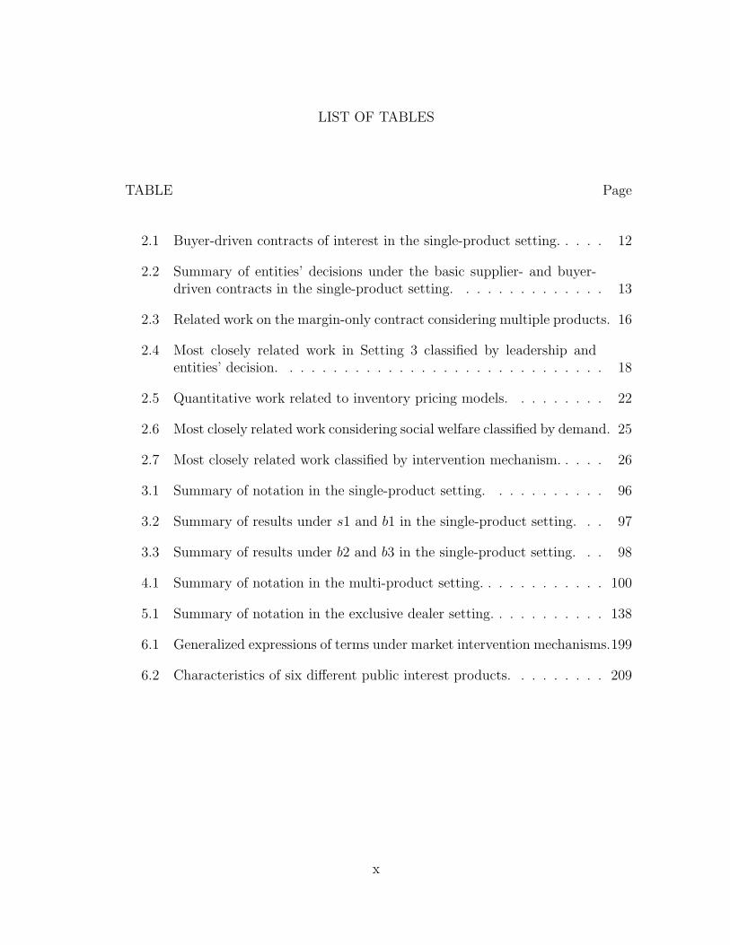
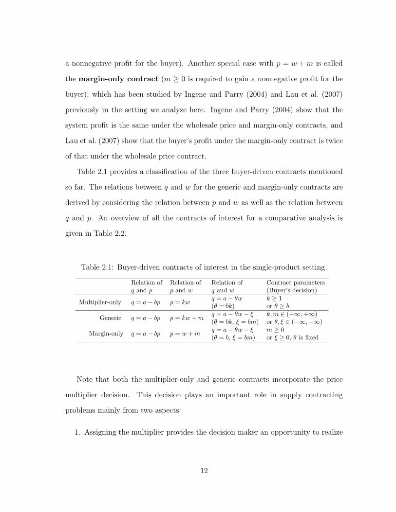
Table 2.1 provides a classification of the three buyer-driven contracts mentioned
so far. The relations between q and w for the generic and margin-only contracts are
derived by considering the relation between p and w as well as the relation between
q and p. An overview of all the contracts of interest for a comparative analysis is
given in Table 2.2.
Table 2.1: Buyer-driven contracts of interest in the single-product setting.
Relation of Relation of Relation of Contract parametersq and p p and w q and w (Buyer’s decision)
Multiplier-only q = a− bp p = kwq = a− θw k ≥ 1(θ = bk) or θ ≥ b
Generic q = a− bp p = kw +mq = a− θw − ξ k,m ∈ (−∞,+∞)(θ = bk, ξ = bm) or θ, ξ ∈ (−∞,+∞)
Margin-only q = a− bp p = w +mq = a− θw − ξ m ≥ 0(θ = b, ξ = bm) or ξ ≥ 0, θ is fixed
Note that both the multiplier-only and generic contracts incorporate the price
multiplier decision. This decision plays an important role in supply contracting
problems mainly from two aspects:
1. Assigning the multiplier provides the decision maker an opportunity to realize
12

Table 2.2: Summary of entities’ decisions under the basic supplier- and buyer-drivencontracts in the single-product setting.
Leader Contract Supplier’s decision Buyer’s decisionSupplier Wholesale price Wholesale price w Quantity q
BuyerMargin-only Wholesale price w Margin m
Multiplier-only Wholesale price w Multiplier kGeneric Wholesale price w Multiplier k and Margin m
more profit (Irmen (1997)a, Tyagi (2005)b, Ertek and Griffin (2002), and Liu
and Cetinkaya (2009)c); and
2. The multiplier represents a practicable profit-driven measure (Liu and Cetinkaya
(2009)) commonly used in the retail industry. In the retail industry, the buyer’s
multiplier p/w and its variants have been commonly used as practicable profit-
driven measures for buyers, according to surveys and articles on industry ap-
plications (e.g., Steiner (1973) and Hall et al. (1997)). The variants of the
multiplier include gross profit margin percentage (GPMP), which is defined as
(unit price- unit purchasing cost)/unit price = (p− w)/p = 1− w/p (Liu and
Cetinkaya (2009)), and the percentage price margin (Tyagi (2005)).
Overall, we consider the basic bilateral monopolistic setting and propose a new
aIrmen (1997) investigates the single-product setting under Nash competition (Fudenberg andTirole (1991)), under which the supplier and buyer move and make decisions simultaneously. Theauthor proves that the retail price is lower and the buyer’s profit is higher if both entities competeon the percentage price margins (i.e., the price multiplier minus one) than if they compete on theprice margins.
bTyagi (2005) considers a multi-product channel where multiple suppliers sell multiple productsthrough a common buyer. The author considers a buyer-driven contract under which the buyerdecides the percentage price margin, i.e., (unit retail price - unit wholesale price)/unit wholesaleprice = (p− w)/w = p/w − 1. The contract is obviously equivalent to the multiplier-only contractunder which the buyer decides the multiplier, i.e., p/w. Tyagi (2005) shows that it is better for thebuyer to decide the percentage price margin than to decide the price margin m = p−w. However,the paper does not show how to derive the optimal contract.
cErtek and Griffin (2002) and Liu and Cetinkaya (2009) demonstrate that the buyer is betteroff by assigning the price multiplier than the price margin decision in single-product channels.
13
contract in the buyer-driven channel called the generic contract. The contract has
a more general pricing scheme than the two existing buyer-driven contracts in the
literature: the margin-only and the multiplier-only contracts. The generic contract
reduces to the margin-only contract when k = 1 and it reduces to the multiplier-only
contract when m = 0. We compare the generic contract with other buyer-driven
contracts in the literature and provide evidence that the generic contract has better
contractual performance than others from several aspects. We demonstrate that the
generic contract is not only optimal for the system and the buyer, it also benefits
consumers and even the supplier.
2.2 Literature related to Setting 2
In the multi-products setting, the supplier’s decisions pertain to the wholesale
prices w1 and w2, and the buyer’s decisions pertain to the order quantities q1 and q2
and the retail prices p1 and p2. The order quantities are dictated by the more general
demand function that depends linearly on the retail prices following qi = a−αpi+βpj
(α > β ≥ 0, i, j = 1, 2, and i = j), where a, α, and β are the parameters of the
demand function.
This type of demand function has been frequently used in the literature on price
competition (e.g., McGuire and Staelin (1983), Choi (1991), Choi (1996), Trivedi
(1998), Pan et al. (2010), and Wu et al. (2012)). In the multi-product setting of
interest, price competition between the substitutable products results from cross-
price effects, where each product’s demand depends on both products’ retail prices.
Hence, the demand function is known as the “symmetric linear demand function
with cross-price effects”, which is the special case of the generalized “linear demand
function with cross-price effects” (e.g., Pashigian (1961), Ingene and Parry (1995),
Tyagi (2005), and Yang and Zhou (2006)). The symmetry assumption for products’
14

demands has been widely adopted in the literature on channel management to keep
the problem formulation simple.
In the supplier-driven multi-product setting, Bresnahan and Reiss (1985) and
Yang and Zhou (2006) consider the wholesale price contract. Bresnahan and Reiss
(1985) make the first attempt to extend the single-product setting by considering
one supplier selling multiple substitutable products to one buyer. Although they
show a property that the buyer’s profit is one-half the supplier’s profit if demand is
linear, they do not characterize the optimal contract explicitly as we do. Yang and
Zhou (2006) consider a similar setting to ours with the exceptions that the supplier’s
wholesale price is not differentiated by products and they do not consider the buyer’s
distribution cost. More importantly, both studies only analyze the channel from the
supplier’s perspective and do not consider any buyer-driven channel.
In this dissertation we take the wholesale price contract as the benchmark supplier-
driven contract when we compare supplier- and buyer-driven contracts, because it has
been widely applied in the supplier-driven price competition models (e.g., McGuire
and Staelin (1983), Ingene and Parry (1995), Saggi and Vettas (2002), Yang and
Zhou (2006), and Adida and DeMiguel (2011)), as well as used as a benchmark to
evaluate buyer-driven contracts (e.g., Choi (1991), Trivedi (1998), Ertek and Griffin
(2002), Tyagi (2005), Pan et al. (2010), and Wu et al. (2012)). Its prevalence is
mainly due to the less cost than other contracts, e.g., the revenue-sharing contract
(Pan et al. (2010)) and the quantity discount contract (Jeuland and Shugan (1983)),
which require more information exchanged between entities.
To the best of our knowledge, the buyer-driven channel has not been analyzed
in the multi-product setting of interest. Several existing papers on buyer-driven
channels have considered the margin-only contract as summarized in Table 2.3 that
provides an overview of the related work on the contract considering multiple prod-
15

ucts. However, the papers in Table 2.3 consider different multi-product problem
settings than ours, i.e., with either multiple suppliers and/or multiple buyers, and
their results cannot be directly applied to our setting. Also, although all the pa-
pers in Table 2.3 make an attempt to investigate the benefit of leadership, they do
not consider the generic and multiplier-only contracts with the exception of Tyagi
(2005)b.
Table 2.3: Related work on the margin-only contract considering multiple products.
Our work (one-supplier-one-buyer) One-supplier-multi-buyer
N/APan et al. (2010)Wu et al. (2012)
Multi-supplier-one-buyer Multi-supplier-multi-buyerChoi (1991)
Lee and Staelin (1997)Tyagi (2005)
Pan et al. (2010)
Choi (1996)Lee and Staelin (1997)
Trivedi (1998)
Overall, we consider three different scenarios in the multi-product setting: sym-
metric two-product, symmetric n-product (n ≥ 2), and asymmetric two-product
scenarios. We focus on analyzing the generic contract in the multi-product setting
with three different scenarios while also consider the wholesale price contract by in-
corporating the buyer’s reservation profit. We show that the optimal generic contract
is easy to calculate even in the asymmetric two-product setting. Furthermore, we
prove that a contractual problem in a symmetric n-product (n ≥ 2) setting can be
reduced to a single-product setting. Hence, in the multi-product setting of interest,
without solving an n-product contractual problem, one can directly use the results
derived in Setting 1 to identify the optimal contract of interest in Setting 2.
16

2.3 Literature related to Setting 3
In practice, the exclusive dealer setting can be seen in many industries. It is par-
ticularly applicable in the automobile industry, where an automobile manufacturer
usually distributes products through its own dealer (Bresnahan and Reiss (1985))
and the manufacturer-dealer pairs in different brands compete on substitutable ve-
hicles. This channel structure also represents other numerous diverse markets, e.g.,
sewing machines, agricultural machinery, and gasoline (Ridgway (1969)).
The comparative analysis of supplier- and buyer-driven contracts on the exclu-
sive dealer setting also has practical importance. It is because in this setting two
manufacturer-dealer pairs distribute two products exclusively and compete with each
other on retail prices and quantities. Each manufacturer-dealer pair forms a vertical
strategic alliance that the manufacturer provides a product to the dealer exclusively
(Bresnahan and Reiss (1985)). Due to the exclusiveness, selecting the right partner
to become a pair is especially important for both entities, and, hence, leadership
and contract settings between the two entities are obviously also important to their
profitabilities. Hence, the comparison of the supplier- and buyer-driven channels is
important due to the simultaneous existence of vertical strategic alliance and hori-
zontal competition.
Next, we proceed with a detailed discussion of the literature on the exclusive
dealer setting and on related contracts in the following two streams:
1. Work related to this setting classified by leadership and entities’ decisions, and
2. Literature that supports the use of the wholesale price contract with Cournot
competition as the benchmark supplier-driven contract.
In the first stream, Table 2.4 lists the most related work to the exclusive dealer
setting classified by leadership and entities’ decisions under a contract. The main
17

Table 2.4: Most closely related work in Setting 3 classified by leadership and entities’decision.
Leadership Work Supplier’s decision Buyer’s decision
Supplier-driven
McGuire and Staelin (1983) Wholesale price Retail priceLee and Staelin (1997) Margin Margin
Trivedi (1998) Wholesale price MarginWu and Mallik (2010) Wholesale price Retail price
Buyer-drivenChoi (1996) Wholesale price Margin
Lee and Staelin (1997) Margin MarginTrivedi (1998) Wholesale price Margin
Zhang et al. (2012) Wholesale price Margin
difference between contracts relies in the different decisions. As we can see, all the
studies in Table 2.4 assume decisions of interest for entities are related to prices.
That is, suppliers decide either the wholesale prices or the manufacture margins
(i.e., difference of the wholesale price and the production cost), and buyers decide
either the retail prices or the price margins (i.e., difference of the retail price and the
wholesale price). While McGuire and Staelin (1983), Lee and Staelin (1997), Trivedi
(1998), and Zhang et al. (2012) study the exclusive dealer setting, Choi (1996) and
Wu and Mallik (2010) consider two-supplier-two-buyer settings different than ours:
Choi (1996) considers the duopoly common retailer channel, where each supplier sells
a product to both buyers with cross sales. Wu and Mallik (2010) consider a setting
where one retailer is owned by one manufacturer under vertical integration and the
other retailer is privately owned.
In fact, McGuire and Staelin (1983) point out that margin decisions can be easily
rescaled to price decisions. Therefore, all the buyer-driven contracts in Table 2.4
are equivalent to the margin-only contract in terms of the equilibrium outcomes.
Specifically, Lee and Staelin (1997), Trivedi (1998), and Zhang et al. (2012) study the
margin-only contract under symmetric assumptions in this setting. All the supplier-
driven contracts in Table 2.4 are equivalent to the wholesale price contract with
18

Bertrand competition, under which the suppliers decide the wholesale prices and then
the buyers decide the retail prices, recalling the definition of Bertrand competition
in Section 1.3.
Regarding the comparative analysis between leaderships, Lee and Staelin (1997)
and Trivedi (1998) demonstrate that each entity is better off to possess leadership.
Lee and Staelin (1997) show that the retail prices and system profits under different
leaderships are the same, i.e., the system efficiency is independent of whether the
suppliers or the buyers play as channel leaders. Lee and Staelin (1997) also claim
that the suppliers and buyers’ profits are symmetric under different leaderships, i.e.,
the leaders’ profits are the same under both leaderships and so as the followers’
profits. Focusing on the duopoly common retailer channel, Choi (1996) shows that
each entity is better off to possess leadership.
In the second stream, as a classic economic model, Bertrand competition de-
scribes a competition structure in which entities decide prices simultaneously, as we
mentioned earlier. Another commonly used economic model, Cournot competition,
describes interactions between entities that set quantities simultaneously. Recall that
the seminal work of Cournot and Bertrand competition goes back to the nineteenth
century by Cournot (1838) and Bertrand (1883), respectively.
A comparison of Cournot and Bertrand competition (i.e., Bertrand-Cournot com-
parison) appears since Singh and Vives (1984) on a one-tier channel. Singh and Vives
(1984) demonstrate the standard conclusion in regard to the comparison. The con-
clusion is that higher prices, lower quantities, and higher profits are obtained in
Cournot than Bertrand and mixed Cournot-Bertrand competition for duopolies if
products are substitutes with linear demand functions. Using a geometric approach,
Cheng (1985) confirms that it is better for duopoly entities to choose a quantity strat-
egy (Cournot competition) than a price strategy (Bertrand competition) if goods are
19

substitutes with given costs (i.e., wholesale prices). Vives (1985) extends the stan-
dard conclusion to oligopolies with arbitrary numbers of entities and more general
demand functions in a symmetric setting. The robustness of the standard conclusion
has been intensely investigated in the economic literature by considering variations of
problem settings, e.g., cost asymmetries, quality difference (Hackner (2000)), mixed
duopolies between private and public firms (Matsumura and Ogawa (2012)).
Although all the literature mentioned above focuses on one-tier channels, the
standard conclusion can be applied to the two-tier channel in the following way. In
a two-tier supplier-buyer channel, after wholesale prices are determined by the sup-
plier(s), the buyers face the same problem as that in a one-tier channel, and, hence,
it is always better for the buyers to compete on quantities (i.e., Cournot compe-
tition) according to the standard conclusion assuming that the buyers are rational
decision makers. Since the buyers are followers who are at the liberty of choosing
a competition strategy after observing wholesale prices, Cournot competition would
be always implemented. Limited work explicitly examines two-tier channels. Man-
asakis and Vlassis (2014) consider the exclusive dealer setting with a more general
objective function for the suppliers. Consistent with the results in one-tierm chan-
nels, they show that Cournot competition is the equilibrium strategy between the
buyers while Bertrand competition can never be an equilibrium strategy. This result
directly supports the use of the wholesale price contract with Cournot competition
as the benchmark contract in the supplier-driven channel.
As we can see, Cournot-Bertrand comparison in one-tier channels has been fully
examined in prior literature, and the comparison under the wholesale price contract
based on downstream entities’ profits in two-tier channels can be also derived ac-
cordingly. However, how the competition strategy adopted by downstream entities
(i.e., buyers) affects upstream entities’ profits (i.e., supplier-tier profit) and system
20

efficiency has not been paid enough attention.
Overall, we currently focus on the buyer-driven channel. While only the margin-
only contract under symmetric assumptions has been studied in the exclusive dealer
setting, we examine the more general contract (the generic contract) under the fully
asymmetric assumption.
2.4 Literature related to Setting 4
We consider a price-setting newsvendor facing stochastic multiplicative demand
in the social welfare setting. Two streams of literature provide background for our
work:
• The empirical work (e.g., Tellis (1988), Mulhern and Lenone (1991), and Hoch
et al. (1995)) supporting the wide applicability of multiplicative demand, and
• The quantitative work on inventory pricing models.
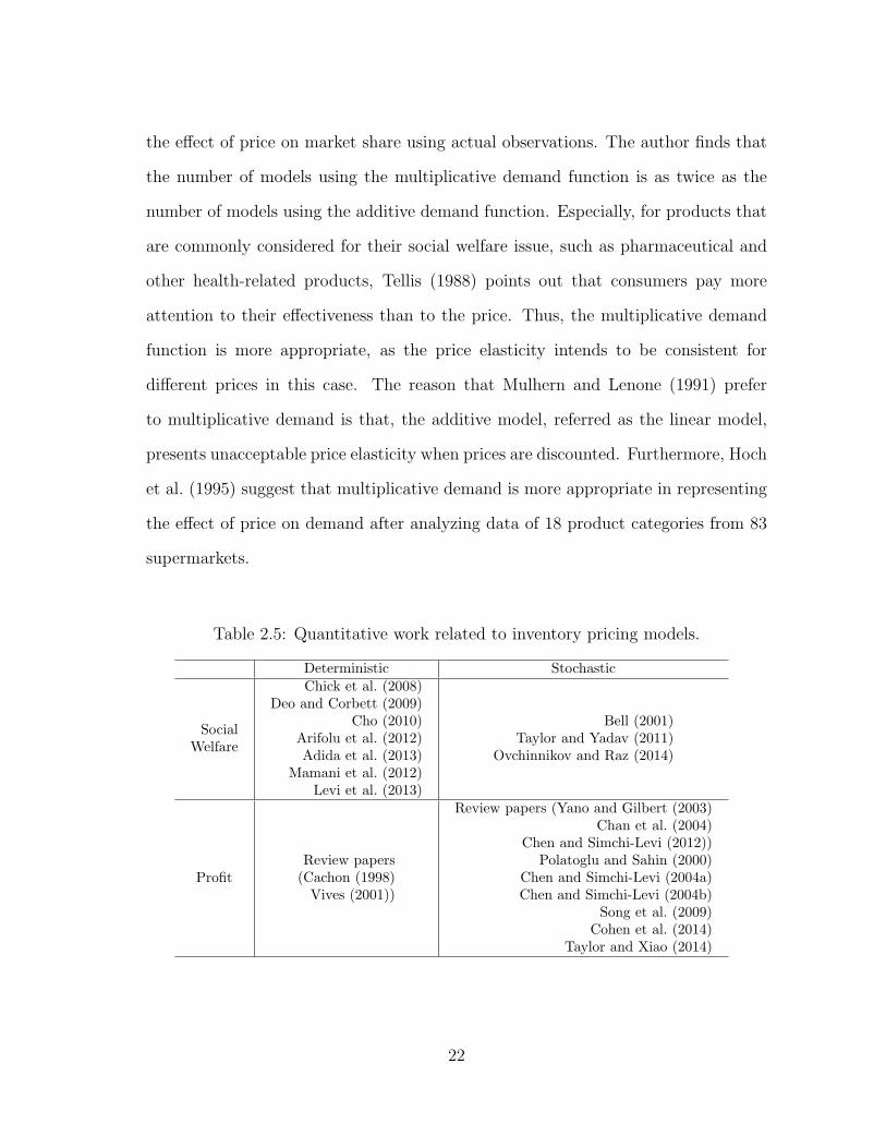
The existing quantitative work on inventory pricing models can be roughly clas-
sified by the optimization objective and by the demand, as shown in Table 2.5. In
the interest of brevity, our emphasis is on previous work that motivates our problem
setting (social welfare and multiplicative demand) by omitting details of less rela-
tive work, such as profit-maximization models under deterministic demand, on the
bottom left hand side of Table 2.5. We refer readers to review papers in this area,
including Cachon (1998) and Vives (2001). In the sequel, we will first review both
the empirical and quantitative work that supports the application of multiplicative
demand, and then review the exiting work focusing on social welfare problems.
Substantial evidence for the importance of multiplicative demand is provided by
the empirical work (e.g., Tellis (1988), Mulhern and Lenone (1991), and Hoch et al.
(1995)). Specifically, Tellis (1988) reviews 424 models from 42 studies on estimating
21
the effect of price on market share using actual observations. The author finds that
the number of models using the multiplicative demand function is as twice as the
number of models using the additive demand function. Especially, for products that
are commonly considered for their social welfare issue, such as pharmaceutical and
other health-related products, Tellis (1988) points out that consumers pay more
attention to their effectiveness than to the price. Thus, the multiplicative demand
function is more appropriate, as the price elasticity intends to be consistent for
different prices in this case. The reason that Mulhern and Lenone (1991) prefer
to multiplicative demand is that, the additive model, referred as the linear model,
presents unacceptable price elasticity when prices are discounted. Furthermore, Hoch
et al. (1995) suggest that multiplicative demand is more appropriate in representing
the effect of price on demand after analyzing data of 18 product categories from 83
supermarkets.
Table 2.5: Quantitative work related to inventory pricing models.
Deterministic Stochastic
SocialWelfare
Chick et al. (2008)Deo and Corbett (2009)
Cho (2010)Arifolu et al. (2012)Adida et al. (2013)
Mamani et al. (2012)Levi et al. (2013)
Bell (2001)Taylor and Yadav (2011)
Ovchinnikov and Raz (2014)
ProfitReview papers(Cachon (1998)Vives (2001))
Review papers (Yano and Gilbert (2003)Chan et al. (2004)
Chen and Simchi-Levi (2012))Polatoglu and Sahin (2000)
Chen and Simchi-Levi (2004a)Chen and Simchi-Levi (2004b)
Song et al. (2009)Cohen et al. (2014)
Taylor and Xiao (2014)
22

On the bottom right hand side of Table 2.5, the literature on inventory pricing
models using stochastic demand functions is vast. The work in this area has been
reviewed by Yano and Gilbert (2003), Chan et al. (2004), and Chen and Simchi-Levi
(2012). The models in this stream can be divided into two groups based on how the
uncertainty is modeled in the demand function, using additive demand and multi-
plicative demand. A large number of studies consider multiplicative demand (e.g.,
Polatoglu and Sahin (2000), Chen and Simchi-Levi (2004a), Chen and Simchi-Levi
(2004b), Song et al. (2009), and Taylor and Xiao (2014)). Though these papers are
devoted to profit maximization problems, they definitely support the use of multi-
plicative demand. In addition, the empirical importance of multiplicative demand
has also been noticed by other analytical work, such as Cachon and Kok (2007),
Driver and Valletti (2003), and Huang and Van Mieghem (2013). Specifically, Ca-
chon and Kok (2007) argue that the multiplicative function, especially in the forms
of D(p, ξ) = x(ξ)αp−β and D(p, ξ) = x(ξ)αe−βp, fits actual data better than the
additive demand function. In the continuous discussion on which function is more
realistic, Driver and Valletti (2003) prefer to the multiplicative demand, as the price
elasticity of demand remains constant to any demand realization. This favor is also
supported by Huang and Van Mieghem (2013). Cohen et al. (2014) consider both
additive and multiplicative demand in a problem where a retailer sells a public in-
terest good and the government applies the rebate mechanism to stimulate the sale
to achieve a given target level. They examine how demand uncertainty (additive
and multiplicative) impacts optimal decisions of the government, industry, and con-
sumers. Our work is different with Cohen et al. (2014)’s work in that we consider
impacts of demand uncertainty on decisions maximizing social welfare, while they
consider the impacts on decisions on achieving a given target sales level.
23

Besides its applicability, the theoretical importance of the multiplicative demand
cannot be ignored as well. Several commonly-used demand functions in stochas-
tic models are multiplicative, e.g., the willingness-to-pay model (e.g., Kocabiyikoglu
and Popescu (2011)), referred as the reservation-price model (e.g., Van Ryzin (2005)).
The reservation-price model is critical in representing demand for a new product or
an existing product using demand forecasts (e.g., Kalish (1985)). Argued by Ko-
cabiyikoglu and Popescu (2011), both the exponential model d(p) = e(z−bp) and the
semilogarithmic function popularly used in the marketing literature, are classified as
or can be transformed into the multiplicative specification. In addition, managerial
insights are usually different respective of demand function, and some of the insights
are even contrasting (e.g., Driver and Valletti (2003), and Salinger and Ampudia
(2011)). To complement the existing work on additive demand and for the com-
parative analysis, it is necessary to study multiplicative demand and investigate the
impact of demand uncertainty on decisions in the social welfare setting.
As this dissertation concentrates on the operational issues in the social welfare
setting, we proceed with a detailed review on existing work in the operation man-
agement area, while the fundamental work on the social welfare in economics (e.g.,
Arrow (1950) and Andersen (1977)) will be not our emphasis. In the social welfare
setting of interest, the newsvendor model is considered by Taylor and Yadav (2011)
and Ovchinnikov and Raz (2014). Taylor and Yadav (2011) consider both the price-
fixed and price-setting newsvendor problems with the additive demand, and Ovchin-
nikov and Raz (2014) also consider the additive demand. With different objectives,
Ovchinnikov and Raz (2014) aim to maximize the expected social welfare, while Tay-
lor and Yadav (2011) are interested in maximizing both the donor’s expected profit
and the expected social welfare. Bell (2001) incorporates the demand uncertainty in
another way by assuming demand depending on consumers’ expected surplus. Prior
24

work on social welfare issues assuming deterministic demand is comparatively rich,
as shown in Table 2.6. Most of the work concentrates in the vaccine market with the
random production yield and deterministic demand of vaccine, while assuming dif-
ferent problem settings. For example, Cho (2010) considers a multi-period problem,
Arifolu et al. (2012) incorporate the consumption externality, and Adida et al. (2013)
consider the effect of network and the consumers’ purchase preference. Mamani et al.
(2012) assume the deterministic demand depending on both price and coverage of
the product.
Table 2.6: Most closely related work considering social welfare classified by demand.
Deterministicdemand
Chick et al. (2008) (random production yield)Deo and Corbett (2009) (random production yield)
Cho (2010) (random production yield)Arifolu et al. (2012) (random production yield)Adida et al. (2013) (random production yield)
Mamani et al. (2012) (demand depending on price and coverage)Levi et al. (2013) (random production yield)
Stochasticdemand
Bell (2001) (demand depending on consumers’ surplus)Taylor and Yadav (2011) (price-fixed/setting and additive)
Ovchinnikov and Raz (2014) (price-setting and additive)Our work (price-setting and multiplicative)
As intervention mechanisms play an important role in coordinating the price and
quantity decisions for a public interest good, the work related to social welfare can be
also classified based on the type of intervention, as shown in Table 2.7. Specifically,
Taylor and Yadav (2011), Adida et al. (2013), and Ovchinnikov and Raz (2014)
employ the subsidies (cost subsidies and purchase subsidies), the rebates (consumer
rebates and sales subsidies) and their combination. Mamani et al. (2012) adopt
the taxes, the subsidies, and their combination. Regards to the effectiveness of a
single intervention, Ovchinnikov and Raz (2014) observe that the consumer rebate
25

is better than the cost subsidy in terms of the less social welfare loss when either
price or quantity is coordinated. Taylor and Yadav (2011) have a similar result
that the sales subsidy is better for both donors and the whole society under specific
conditions. Respect to joint interventions, Adida et al. (2013), Mamani et al. (2012)
and Ovchinnikov and Raz (2014) all prove combinations of interventions achieving
the system coordination and maximizing the expected social welfare. We summarize
the most related work to our work in Table 2.7 by emphasizing our differences on
intervention mechanisms of interest.
Table 2.7: Most closely related work classified by intervention mechanism.
Regulation Market interventionTaxes Subsidies Rebates
Ovchinnikov and Raz (2014) ✓ ✓Taylor and Yadav (2011) ✓ ✓
Adida et al. (2013) ✓ ✓Mamani et al. (2012) ✓ ✓
Our work ✓ ✓ ✓ ✓
Realizing the empirical and theoretical importance of the multiplicative demand
and the significance of social welfare for marketing a public interest good, to the best
of our knowledge, this dissertation is the first to combine the two characteristics and
to investigate government intervention mechanisms that maximize the expected so-
cial welfare. As mentioned earlier, we prove that the multiplicative demand function
is feasible in modeling the social welfare. The proof is built on results by Krishnan
(2010) and Mas-Colell et al. (1995).
Overall, we revisit Ovchinnikov and Raz (2014) by considering a social welfare
setting, in which a public interest good is distributed by a newsvendor-type seller to
26

consumers with stochastic demand depending on retail price under the multiplicative
demand function. We propose two new government regularity intervention and one
new market intervention for channel coordination to maximize the expected social
welfare. We investigate contractual performance under various interventions in terms
of effectiveness, efficiency and the government cost.
27

3. PRELIMINARIES AND THE GENERIC CONTRACT
3.1 Setting 1. The basic bilateral monopolistic contractual setting (a.k.a.
single-product setting)
We consider the basic bilateral monopolistic setting, i.e., the supplier-buyer
channel, with a single product and price-sensitive deterministic demand illustrated in
Figure 3.1 and referred as the single-product setting here. The buyer’s price-sensitive
demand function is given by
q = a− bp, (3.1)
where q and p denote the demand quantity and retail price, respectively. Naturally,
0 ≤ p ≤ a/b, so that q ≥ 0. Parameter a, a > 0, represents the market potential
which is the demand when price approaches zero (Swartz and Iacobucci (2000)).
Hence, a also represents the part of demand that is not affected by price (Adida
and Perakis (2010)). Parameter b, b > 0, represents the sensitivity of demand with
respect to price (Ingene and Parry (2004) and Adida and Perakis (2010)). Hence, b
measures how the demand is affected by price. The decisions of interest to the buyer
are q and p. Clearly, q dictates the buyer’s order quantity, which in turn, is filled by
the supplier at wholesale price, denoted by w, so that the decision of interest to the
supplier is w. The notation introduced so far and used frequently in the remainder
of this chapter is summarized in Table 3.1.
BuyerSupplierq = a � bp
w p
Figure 3.1: The basic bilateral monopolistic contractual setting.
28

We are interested in studying contractual settings related to the buyer’s decisions
(i.e., p and q) as well as the supplier’s decision (i.e., w) in this setting. Of particular
interest is an explicit comparison of buyer- and supplier-driven contracts as discussed
in the next section.
3.2 Supplier- and buyer-driven contracts
In the supplier-driven channel, the supplier moves first to specify a contract and
then the buyer makes decisions accordingly. In contrast, in the buyer-driven channel,
the buyer moves first to specify a contract and then the supplier makes decisions
accordingly (Liu and Cetinkaya (2009)).
For an explicit comparison of buyer- and supplier-driven channels, we consider
four specific contracts. Namely, we consider the wholesale price contract, denoted by
s1, in the supplier-driven channel, and the margin-only, multiplier-only, and generic
contracts, denoted by b1, b2, and b3, respectively, in the buyer-driven channel:
s1. Under the wholesale price contract, the supplier decides w and then the buyer
decides p.
b1. Under the margin-only contract, the buyer decides the price margina, denoted
by m, m ≥ 0, representing the difference between the retail and wholesale
prices, while also committing that the retail price would be set such that p =
w+m and the order quantity would be set such that q = a−bp = a−b(w+m)b.
Next, the supplier decides w.
b2. Under the multiplier-only contract, the buyer decides the price multiplierc, de-
aThe term price margin is used because m ≥ 0 adds a per unit profit to the wholesale price. Asshown later, under b1, m satisfies (3.22).
bAlthough we mention that the buyer commits on both relationships for p and q, we will showlater that it suffices for the buyer to commit only on the latter relationship regarding q so thatthere is no credibility issue under this contract.
cThe term price multiplier is used because k ≥ 1 marks up the wholesale price through multi-
29

noted by k, k ≥ 1, representing the ratio of the retail and wholesale prices,
while also committing that the retail price would be set such that p = kw and
the order quantity would be set such that q = a − bp = a − bkwb. Next, the
supplier decides w.
b3. Under the generic contract, the buyer decides on the valuesd of k, k ∈ ℜ, and
m, m ∈ ℜ, while also committing that the retail price would be set such that
p = kw + m and the order quantity would be set such that q = a − bp =
a− b(kw +m)b. Next, the supplier decides w.
Contracts s1, b1, and b2 are commonly utilized in practice and analyzed in pre-
vious literaturee. Contract b3 is inspired by b1 and b2 in an attempt to propose a
more general pricing scheme and analyzed here for the sake of generality. We are
interested in computing the optimal contract parameters under s1, b1, b2, and b3.
To this end, we develop basic optimization models, and we utilize the principles of
Stackelberg games because the contracting processes are representative of sequential
leader-follower games (see Chapter 3 of Fudenberg and Tirole (1991)).
3.3 Profit functions
In the single-product setting, using (3.1), the supplier’s profit function is given
by
πs = (w − s)q = (w − s)(a− bp), (3.2)
plication. As shown later, under b2, k also satisfies (3.49).dObserve that, under b3, m can be positive or negative representing a margin (mark-up) or
rebate (mark-down). Likewise, under b3, k is allowed to be positive or negative for the sake ofgenerality. However, it is shown later that due to the natural and practical assumptions of theproblem setting at hand (e.g., see assumption (3.5)), k and m are such that (3.60) and (3.71) hold.Also, the optimal value of k satisfies k ≥ 1.
eFor example, s1 has been studied by Corbett et al. (2004) among others; b1 has been studiedby Lau et al. (2007) among others; and b2 has been studied by Liu and Cetinkaya (2009) amongothers. The details of earlier work on these contracts as they apply to our work are given in Sections3.4 and 3.2.
30

where s is the supplier’s unit production cost, s ≥ 0. The buyer’s profit function is
given by
πb = (p− w − c)q = (p− w − c)(a− bp), (3.3)
where c is the buyer’s unit distribution cost, c ≥ 0. The system profit function is
given by
Π = πs + πb = (p− s− c)q = (p− s− c)(a− bp). (3.4)
Recalling (3.1), (3.2), and (3.3), in order to guarantee q ≥ 0, πb ≥ 0, and πs ≥ 0, we
assume p ≤ a/b, w ≥ s, and p ≥ w + c so that
s+ c ≤ w + c ≤ p ≤ a
b. (3.5)
We pay particular attention to ensure that the contractual problems at hand
lead to nonnegative profits πb, πs, and Π for the sake of practical realism. We
also incorporate the notion of reservation profits, denoted by π−b ≥ 0 for the buyer
and π−s ≥ 0 for the supplier, so that not only the profits are nonnegative but also
they exceed minimum expectations of the entities involved. Then, considering the
fact that s1 is a supplier-driven contract, the buyer would not accept s1 unless the
buyer’s corresponding profit exceeds π−b . Likewise, considering the fact that b1 (b2
and b3) is a buyer-driven contract, the supplier would not accept b1 (b2 and b3)
unless the supplier’s corresponding profit exceeds π−s .
We are primarily interested in the more general case where all external model
parameters, i.e., a, b, s, c, π−b , and π−
s , are positive. However, when appropriate
or necessary, we comment on the cases where s = 0, π−b = 0, and π−
s = 0 for three
specific reasons to include
• These cases have appeared in the literature (e.g., Corbett and Tang (1999)
31

ignore π−b ≥ 0 under s1 and Lau et al. (2007) assume π−
s = 0 under b1),
• They make practical sense (e.g., the case s = 0 is applicable if the supplier is a
wholesale distributer, i.e., not a manufacturer. Raju and Zhang (2005) assume
s = 0 in a channel with a supplier, a dominant retailer and multiple fringe
retailers.), and
• The technical derivations of optimal contract parameters are different (e.g., see
the derivations under b2 for s = 0 and s > 0).
3.3.1 Centralized problem
Under centralized control, p is decided by the central planner to maximize the
system profit Π in (3.4). This is a hypothetical assumption but it is useful to obtain
an upper bound on the system profit so that we have a benchmark on the overall
performance under the contracts of interest. Hence, using (3.4) and assumption (3.5),
the centralized optimization problem can be stated as
(Pc) : maxs+c≤p≤a/b
Π = (p− s− c)q = (p− s− c)(a− bp).
Clearly, w is immaterial for Π in (3.4), and, hence, by assumption (3.5), we are only
interested in p values that satisfy
s+ c ≤ p ≤ a
b. (3.6)
We refer to (3.6) as the main constraint on the decision variable p of the central-
ized problem. Now, recalling (3.1) and considering (3.6), we note that
0 ≤ q ≤ a− b(s+ c). (3.7)
32

Also, we note that (3.6) as well as (3.7) assure that Π in (3.4) is nonnegative. In
fact, this is the leastf the centralized decision maker should target.
Using (3.4), note that
dΠ
dp= a− 2bp+ b(s+ c) and (3.8)
d2Π
dp2= −2b < 0.
It is easy to see that Π is concave in p and setting dΠ/dp = 0 in (3.8) leads to
pc =a+ b(s+ c)
2b. (3.9)
Observe that pc defined in (3.9) is the centralized optimal retail price. This
is because by assumption (3.5),
a
b− pc =
a− b(s+ c)
2b≥ 0 and
pc − (s+ c) =a− b(s+ c)
2b≥ 0,
so that pc in (3.9) is realizable over the region (3.6). Using (3.1) and (3.9), the
centralized optimal order quantity is given by
qc =a− b(s+ c)
2. (3.10)
Clearly, by assumption (3.5),
a− b(s+ c)− qc =a− b(s+ c)
2≥ 0,
fAs we have noted earlier, when we develop optimization models for the contracts of interest,we eventually incorporate the notion of reservation profits so that not only the profits are positivebut also they exceed minimum expectations of the entities involved.
33

so that qc defined in (3.10) lies over the region (3.7). Substituting (3.9) in (3.4), the
centralized optimal system profit, denoted by Πc, is given by
Πc =[a− b(s+ c)]2
4b. (3.11)
It is important to note that (Pc) is also solved by Lau et al. (2007) leading to pc
in (3.9) and Πc in (3.11) (see the expressions in (2) on p. 850 of Lau et al. (2007)).
Ingene and Parry (2004) also consider a variant of (Pc) but allowing a more general
cost structure where each entity has a per unit cost as well as a fixed cost. By
setting the fixed costs equal zero, their problem (see the problem in (2.3.2) on p. 35
of Ingene and Parry (2004)) is reduced to (Pc) leading to pc in (3.9) and Πc in (3.11)
(see (2.3.4) on p. 35 and (2.3.6) on p. 36 of Ingene and Parry (2004)).
3.4 Contract-based optimization problems
3.4.1 Wholesale price contract s1
As we have noted in Section 3.2, under s1, the supplier decides w first and then
the buyer decides p. By assumption (3.5), under s1, we are only interested in w and
p values that satisfy
s ≤ w ≤ a
b− c and (3.12)
w + c ≤ p ≤ a
b. (3.13)
Also, recalling (3.1) and considering (3.13), we have
0 ≤ q ≤ a− b(w + c). (3.14)
We refer to (3.12) as the main constraint on the decision variable w of the contract
34

design problem under s1. Also, we note that (3.13) as well as (3.14) assure πb in (3.3)
is nonnegative. In fact, this is the leastf the supplier should consider in designing
the supplier-driven contract s1.
For a given w that satisfies (3.12), using (3.3), we have
πb = (p− w − c)(a− bp),
so that
dπb
dp= a− 2bp+ b(w + c) and (3.15)
d2πb
dp2= −2b < 0.
Clearly, πb is concave in p and setting dπb/dp = 0 in (3.15) leads to
ps1(w) =a+ b(w + c)
2b. (3.16)
Observe that for any w such that (3.12) is true, ps1(w) defined in (3.16) is the
buyer’s optimal response, i.e., the optimal retail price, under s1. This is
because w satisfies (3.12) so that
a
b− ps1(w) =
a− b(w + c)
2b≥ 0 and
ps1(w)− (w + c) =a− b(w + c)
2b≥ 0.
Hence, ps1(w) in (3.16) is realizable over the region (3.13). Substituting (3.16) in
(3.1), the buyer’s optimal order quantity under s1 for a given w that satisfies
35

(3.12) can be written as
qs1(w) =a− b(w + c)
2. (3.17)
Again, since w satisfies (3.12),
a− b(w + c)− qs1(w) =a− b(w + c)
2≥ 0,
so that qs1(w) defined in (3.17) lies over the region (3.14).
Also, given the main constraint (3.12) on the decision variable w, it is easy to
verify that assumption (3.5) holds true for p = ps1(w), where ps1(w) is as defined
in (3.16). Hence, the buyer’s optimal price-quantity response tuple (ps1(w), qs1(w))
does not violate the fundamental assumptions of the problem at hand.
Using (3.16) and (3.17) in (3.2) and (3.3), we have
πs =(w − s)[a− b(w + c)]
2and
πb =[a− b(w + c)]2
4b.
As noted earlier, considering the fact that s1 is a supplier-driven contract, the buyer
would not accept s1 unless the buyer’s corresponding profit exceeds π−b . Then, recall-
ing (3.12) and considering the two above expressions for πs and πb, the supplier’s
optimization problem under s1 can be stated as
(Ps1) : maxs≤w≤a/b−c
πs =(w − s)[a− b(w + c)]
2(3.18)
s.t. πb =[a− b(w + c)]2
4b≥ π−
b . (3.19)
Clearly, (Ps1) makes sense only for reasonable values of π−b . That is, a natural
36
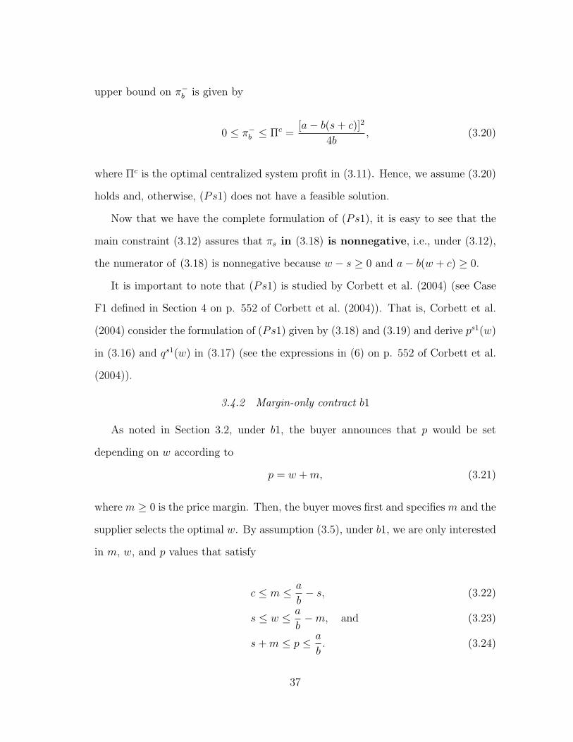
upper bound on π−b is given by
0 ≤ π−b ≤ Πc =
[a− b(s+ c)]2
4b, (3.20)
where Πc is the optimal centralized system profit in (3.11). Hence, we assume (3.20)
holds and, otherwise, (Ps1) does not have a feasible solution.
Now that we have the complete formulation of (Ps1), it is easy to see that the
main constraint (3.12) assures that πs in (3.18) is nonnegative, i.e., under (3.12),
the numerator of (3.18) is nonnegative because w − s ≥ 0 and a− b(w + c) ≥ 0.
It is important to note that (Ps1) is studied by Corbett et al. (2004) (see Case
F1 defined in Section 4 on p. 552 of Corbett et al. (2004)). That is, Corbett et al.
(2004) consider the formulation of (Ps1) given by (3.18) and (3.19) and derive ps1(w)
in (3.16) and qs1(w) in (3.17) (see the expressions in (6) on p. 552 of Corbett et al.
(2004)).
3.4.2 Margin-only contract b1
As noted in Section 3.2, under b1, the buyer announces that p would be set
depending on w according to
p = w +m, (3.21)
where m ≥ 0 is the price margin. Then, the buyer moves first and specifies m and the
supplier selects the optimal w. By assumption (3.5), under b1, we are only interested
in m, w, and p values that satisfy
c ≤ m ≤ a
b− s, (3.22)
s ≤ w ≤ a
b−m, and (3.23)
s+m ≤ p ≤ a
b. (3.24)
37

Also, recalling (3.1) and considering (3.24), we have
0 ≤ q ≤ a− b(s+m). (3.25)
We refer to (3.22) as the main constraint on the decision variablem of the contract
design problem under b1. Also, we note that (3.23) along with (3.24)–(3.25) assure
that πs in (3.2) is nonnegative. In fact, this is the leastf the buyer should consider
in designing the buyer-driven contract b1.
For a given m that satisfies (3.22), using (3.21), πs in (3.2) can be rewritten as
πs = (w − s)q = (w − s)(a− bp) = (w − s)[a− b(w +m)]
so that
dπs
dw= a− 2bw + b(s−m) and (3.26)
d2πs
dw2= −2b < 0. (3.27)
Clearly, πs is concave in w and setting dπs/dw = 0 in (3.26) leads to
wb1(m) =a+ b(s−m)
2b. (3.28)
Observe that for any m such that (3.22) is true, wb1(m) defined in (3.28) is the
supplier’s optimal response, i.e., the optimal wholesale price, under b1.
This is because m satisfies (3.22) so that
a
b−m− wb1(m) =
a− b(s+m)
2b≥ 0 and
wb1(m)− s =a− b(s+m)
2b≥ 0.
38
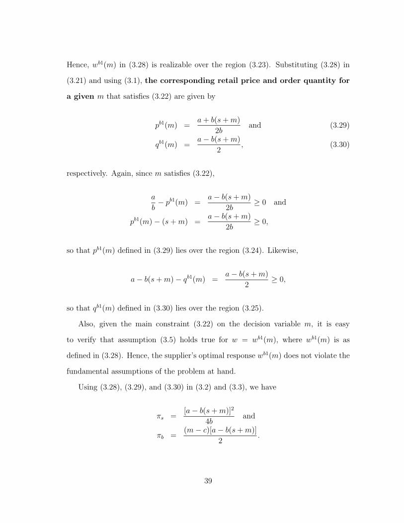
Hence, wb1(m) in (3.28) is realizable over the region (3.23). Substituting (3.28) in
(3.21) and using (3.1), the corresponding retail price and order quantity for
a given m that satisfies (3.22) are given by
pb1(m) =a+ b(s+m)
2band (3.29)
qb1(m) =a− b(s+m)
2, (3.30)
respectively. Again, since m satisfies (3.22),
a
b− pb1(m) =
a− b(s+m)
2b≥ 0 and
pb1(m)− (s+m) =a− b(s+m)
2b≥ 0,
so that pb1(m) defined in (3.29) lies over the region (3.24). Likewise,
a− b(s+m)− qb1(m) =a− b(s+m)
2≥ 0,
so that qb1(m) defined in (3.30) lies over the region (3.25).
Also, given the main constraint (3.22) on the decision variable m, it is easy
to verify that assumption (3.5) holds true for w = wb1(m), where wb1(m) is as
defined in (3.28). Hence, the supplier’s optimal response wb1(m) does not violate the
fundamental assumptions of the problem at hand.
Using (3.28), (3.29), and (3.30) in (3.2) and (3.3), we have
πs =[a− b(s+m)]2
4band
πb =(m− c)[a− b(s+m)]
2.
39

As noted earlier, considering the fact that b1 is a buyer-driven contract, the supplier
would not accept b1 unless the supplier’s corresponding profit exceeds π−s . Hence, we
have the constraint πs ≥ π−s . Then, recalling (3.22) and considering the two above
expressions for πs and πb, the buyer’s optimization problem under b1 can be
stated as
(Pb1) : maxc≤m≤a/b−s
πb =(m− c)[a− b(s+m)]
2(3.31)
s.t. πs =[a− b(s+m)]2
4b≥ π−
s . (3.32)
Clearly, (Pb1) makes sense only for reasonable values of π−s . That is, a natural
upper bound on π−s is given by
0 ≤ π−s ≤ Πc =
[a− b(s+ c)]2
4b, (3.33)
where Πc is the optimal centralized system profit in (3.11). Hence, we assume (3.33)
holds and, otherwise, (Pb1) does not have a feasible solution.
Now that we have the complete formulation of (Pb1), it is easy to see that the
main constraint (3.22) assures that πb in (3.31) is nonnegative, i.e., under (3.22),
the numerator of (3.31) is nonnegative because m− c ≥ 0 and a− b(s+m) ≥ 0.
It is important to note that (Pb1) is studied by Lau et al. (2007) who assume
π−s = 0. That is, Lau et al. (2007) consider πb in (3.31) and derive wb1(m) in (3.28)
(see the expression in (5) on p. 852 of Lau et al. (2007)). Ingene and Parry (2004)
also consider a variant of (Pb1) again assuming π−s = 0 but allowing a more general
cost structure, where each entity has a per unit cost as well as a fixed cost. By setting
the buyer’s fixed cost equal zero, their problem (see the problem in (2.3.29) on p.
39 of Ingene and Parry (2004)) is reduced to (Pb1) with π−s = 0. Hence, qb1(m) in
40

(3.30) is also derived by Ingene and Parry (2004) (see the expression in (2.3.28) on
p. 39 of Ingene and Parry (2004)).
3.4.3 Multiplier-only contract b2
As noted in Section 3.2, under b2, the buyer announces that p would be set
depending on w according to
p = kw, (3.34)
where k ≥ 1 is the price multiplier. Then, the buyer moves first and specifies k and
the supplier selects the optimal w. Substituting (3.34) in (3.1), we have
q = a− bp = a− bkw ≥ 0. (3.35)
By assumption (3.5), we have w ≥ s. Hence, using (3.35),
a− bsk ≥ a− bkw ≥ 0.
Then, under b2, we are only interested in k and w values that satisfy
1 ≤ k ≤ a
bsand (3.36)
s ≤ w ≤ a
bk. (3.37)
Also, using (3.34) in (3.37), we have
sk ≤ p ≤ a
b. (3.38)
41

Then, recalling (3.1) and considering (3.38) leads to
0 ≤ q ≤ a− bsk. (3.39)
We refer to (3.36) as the main constraint on the decision variable k of the contract
design problem under b2. However, unlike in the case of b1, the main constraint (3.36)
along with the accompanying constraints (3.42)–(3.44) do not assure that πb in (3.3)
is nonnegativeg under b2. We address this concern momentarily once we compute
the supplier’s optimal response.
For a given k that satisfies (3.36), using (3.34), πs in (3.2) can be rewritten as
πs = (w − s)q = (w − s)(a− bp) = (w − s)(a− bkw),
so that
dπs
dw= a+ bsk − 2bkw and (3.40)
d2πs
dw2= −2bk < 0. (3.41)
Clearly, πs is concave in w and setting dπs/dw = 0 in (3.40) leads to
wb2(k) =a+ bsk
2bk. (3.42)
Observe that for any k such that (3.36) is true, wb2(k) defined in (3.42) is the
supplier’s optimal response, i.e., the optimal wholesale price, under b2.
gThis is simply because the lower limit of k in (3.36) is specified as k ≥ 1 so that p = kw ≥ w.However, the lower limit k ≥ 1 alone does not assure p = kw ≥ w+ c which is in fact the conditionassuring that πb in (3.3) is nonnegative. We momentarily ignore this more strict lower limit onk but later we establish its equivalent (see (3.46)) and incorporate it in our analysis.
42

This is because k satisfies (3.36) so that
a
bs− wb2(k) =
a− bsk
2bk≥ 0 and
wb2(k)− s =a− bsk
2bk≥ 0.
Hence, wb2(k) in (3.42) is realizable over the region (3.37). Substituting (3.42) in
(3.34) and using (3.1), the corresponding retail price and order quantity for
a given k that satisfies (3.36) are given by
pb2(k) =a+ bsk
2band (3.43)
qb2(k) =a− bsk
2, (3.44)
respectively. Again, since k satisfies (3.36),
a
b− pb2(k) =
a− bsk
2b≥ 0 and
pb2(k)− sk =a− bsk
2b≥ 0,
so that pb2(k) defined in (3.43) lies over the region (3.38). Likewise,
a− bsk − qb2(k) =a− bsk
2≥ 0,
so that qb2(k) defined in (3.44) lies over the region (3.39).
Now, as before, we need to verify that assumption (3.5) holds true for w = wb2(k),
where wb2(k) is as defined in (3.42). Unlike in the case of b1, the main constraint
(3.36) on the decision variable k is not sufficienth for this verification under b2. For
hAlso, see footnote g.
43

this reason, rewriting assumption (3.5) while using (3.42), we need to ensure
s+ c ≤ a+ bsk
2bk+ c ≤ p =
a+ bsk
2b≤ a
b(3.45)
holds true. Examining the above inequalities, it is easy to validate that if the lower
limit of (3.36) is revised such that
k ≥ 1 +2bck
a+ bsk
then (3.45) is ensured. Hence, the main constraint (3.36) needs to be replaced with
1 +2bck
a+ bsk≤ k ≤ a
bs, (3.46)
so that assumption (3.5) holds true for w = wb2(k).
For obvious reasons, we now refer to (3.46) as the main constraint on the decision
variable k of the contract design problem under b2. Using the newly established lower
limit of k in (3.46), we note that
1 +2bck
a+ bsk= k
is equivalent to f(k) = 0 where f(k) is defined as
f(k) = bsk2 + (a− bs− 2bc)k − a. (3.47)
Observe that
df(k)
dk= 2bsk + a− bs− 2bc and
d2f(k)
dk2= 2bs.
44

Hence, f(k) is convex in k. Also, limk→+∞ f(k) → +∞ and f(0) = −a < 0. Function
f(k) is illustrated in Figures 3.2 and 3.3 when the minimizer k∗f of f(k) is positive
and negative, respectively. It is easy to verify that
k∗f = −a− bs− 2bc
2bs(3.48)
so that k∗f ≥ 0 if a − bs − 2bc ≤ 0 and k∗
f < 0 if a − bs − 2bc > 0. As illustrated
in Figures 3.2 and 3.3, for both cases, there exists a unique positive kl such that
f(kl) = 0 so that (3.46) can be rewritten as
kl ≤ k ≤ a
bs. (3.49)
It then follows that, given the final main constraint (3.49) on the decision variable
k, assumption (3.5) holds true for w = wb2(k).
lka−
)(kf
bs
bcbsak f 2
2* −−−= k0
Figure 3.2: An illustration of f(k) in (3.47) when a− bs− 2bc < 0.
45

lka−
)(kf
bs
bcbsak f 2
2* −−−= k
0
Figure 3.3: An illustration of f(k) in (3.47) when a− bs− 2bc > 0.
Using (3.42), (3.43), and (3.44) in (3.2) and (3.3), we have
πs =(a− bsk)2
4bkand
πb =(a− bsk)[a(k − 1) + bk(sk − s− 2c)]
4bk.
Then, recalling (3.49) and considering the two above expressions for πs and πb, the
buyer’s optimization problem under b2 can be stated as
(Pb2) : maxkl≤k≤a/(bs)
πb =(a− bsk)[a(k − 1) + bk(sk − s− 2c)]
4bk(3.50)
s.t. πs =(a− bsk)2
4bk≥ π−
s . (3.51)
Now that we have the complete formulation of (Pb2), it is easy to see that the
main constraint (3.49) assures that πb in (3.50) is nonnegative. This is because
• The first term a − bsk that appears in the numerator of (3.50) is such that
a− bsk ≥ 0 under (3.49), and
• By definition of kl and the properties of f(k) discussed above, the next term
46

that appears in the numerator of (3.50) is such that
a(k − 1) + bk(sk − s− 2c) = bsk2 + (a− bs− 2bc)k − a ≥ 0
under (3.49).
It is important to note that (Pb2) is formulated and solved by Liu and Cetinkaya
(2009) (see (BPBF1) on p. 692 of Liu and Cetinkaya (2009)). That is, they also
derive wb2(k) in (3.42) (see the expression in (4) on p. 691 of Liu and Cetinkaya
(2009)) along with (3.50) and (3.51) (see expressions in (BPBF1) on p. 692 of Liu
and Cetinkaya (2009)).
It is worthwhile to note that the lower limit of k in the main constraint (3.49)
is omitted by Liu and Cetinkaya (2009) as they implicitly assume that π−b = 0 by
arguing that the buyer will not trade if the resulting profit is negative, whereas
we provide the region of k given in (3.49) that guarantees the resulting profit is
nonnegative. As wee have noted earlier (see footnote f), we pay particular attention
to ensure that the contractual problems at hand lead to nonnegative profits for both
entities for the sake of practical realism.
3.4.4 Generic contract b3
As noted in Section 3.2, under b3, the buyer announces that p would be set
depending on w according to
p = kw +m, (3.52)
where k ∈ ℜ is the unconstrained multiplier and m ∈ ℜ is the unconstrained value
representing a margin (mark-up) or rebate (mark-down). Then, the buyer moves
first and decides k and m and the supplier selects the optimal w.
It is important to note that here k ∈ ℜ and m ∈ ℜ are defined as unconstrained
47

values for the sake of generality because the purpose of this contract is to capture
a more general pricing scheme than implied by b1 and b2. As we demonstrate next,
k and m are subject to constraints as in the case of the parameters of the other
contracts (e.g., see the upper/lower bounds given by (3.22) under b1 and given by
(3.49) under b2.)
Substituting (3.52) in (3.1), we have
q = a− bp = a− b(kw +m) ≥ 0, (3.53)
and, hence,
kw +m ≤ a
b. (3.54)
Also, by assumption (3.5), we have
s ≤ w ≤ a
b− c and (3.55)
s+ c ≤ p ≤ a
b. (3.56)
Then, recalling (3.1) and considering (3.56),
0 ≤ q ≤ a− b(s+ c). (3.57)
Given (3.54)–(3.57), for reasons that will become apparent momentarily, let us
consider the cases k ≤ 0 and k > 0, separately:
• If k ≤ 0 then (3.54) and (3.55) imply that k and m should satisfy
k(ab− c)+m ≤ a
b, (3.58)
48
while w, p, and q should satisfy (3.55), (3.56), and (3.57), respectively.
• If k > 0 then (3.54) and (3.55) imply that
sk +m ≤ kw +m ≤ a
b. (3.59)
Using (3.59) along with (3.55) and (3.56), we then conclude that k, m, w, and
p should be such that
sk +m ≤ a
b(3.60)
s ≤ w ≤ a
bk− m
k, and (3.61)
sk +m ≤ p ≤ a
b. (3.62)
Also, recalling (3.1) and considering (3.62), for the case k > 0, we have
0 ≤ q ≤ a− b(sk +m). (3.63)
We then conclude that the natural constraints on the decision variables and
parameters of interest are given
• By (3.55), (3.56), (3.57), and (3.58) if k < 0, and
• By (3.60), (3.61), (3.62), and (3.63) if k > 0.
Initially, we refer to (3.58) and (3.60) as the main constraints on the decision
variables k and m of the contract design problem under b3. Clearly, (3.58) applies
to the case k ≤ 0 whereas (3.60) applies to the case k > 0. Similar to the case of
b2, under b3, (3.58) or (3.60) alone does not assure that πb in (3.3) is nonnegative.
49

We proceed with addressing this concern by first computing the supplier’s optimal
response under b3.
To this end, let us examine πs in (3.2) under b3. For given values of k ∈ ℜ and
m ∈ ℜ, using (3.52), πs in (3.2) can be rewritten as
πs = (w − s)q = (w − s)(a− bp) = (w − s)[a− b(kw +m)], (3.64)
so that
dπs
dw= [a− b(kw +m)]− bk(w − s) and (3.65)
d2πs
dw2= −2bk. (3.66)
For reasons that will become apparent shortly, this end, let us again consider the
cases k ≤ 0 and k > 0, separately:
Case 1: k ≤ 0
In this case, considering (3.66) and using (3.53) and (3.55) in (3.65), it can be
easily verified that πs is convex and increasing in w over the region (3.55). For given
values of k ≤ 0 and m ∈ ℜ such that (3.58) holds, the maximizer of πs in (3.64) is
then given by a/b − c which is the upper limit of (3.55). In turn, using (3.1) and
substituting w = a/b− c in (3.3),
πb = (p− w − c)q =(p− a
b
)(a− bp) = −(a− bp)2
b≤ 0,
regardless of the value of p. Therefore, if k ≤ 0 then the buyer does not make any
profit. Hence, we can discard the case k ≤ 0 and restrict our attention to
the case k > 0.
50

Case 2: k > 0
In this case, it follows from (3.66) that πs is concave in w. Setting dπs/dw = 0
in (3.65) leads to
wb3(k,m) =a+ b(sk −m)
2bk. (3.67)
Now, observe that for given values of k > 0 and m ∈ ℜ such that (3.60) is true,
we have
( a
bk− m
k
)− wb3(k,m) =
a− b(sk +m)
2bk≥ 0 and
wb3(k,m)− s =a− b(sk +m)
2bk≥ 0.
Then, wb3(k,m) defined in (3.67) is the supplier’s optimal response, i.e., the
optimal wholesale price, under b3 because it is realizable over the region (3.61).
Substituting (3.67) in (3.52) and using (3.1), the corresponding retail price and
order quantity for given values of k > 0 and m ∈ ℜ that satisfy (3.60) are
given by
pb3(k,m) =a+ b(sk +m)
2band (3.68)
qb3(k,m) =a− b(sk +m)
2, (3.69)
respectively. Again, since we assume (3.60),
a
b− pb3(k,m) =
a− b(sk +m)
2b≥ 0 and
pb3(k,m)− (sk +m) =a− b(sk +m)
2b≥ 0,
51

so that pb3(k,m) defined in (3.68) lies over the region (3.62). Likewise,
a− b(sk +m)− qb3(k,m) =a− b(sk +m)
2≥ 0,
so that qb3(k,m) defined in (3.69) lies over the region (3.63).
Last but not least, we need to verify that assumption (3.5) holds true for w =
wb3(k,m), where wb3(k,m) is as defined in (3.67). Similar to the case of b2, the main
constraint (3.60) derived earlier is not sufficient to verify this under b3. For this
reason, recalling assumption (3.5) and using (3.67), we need to ensure
s+ c ≤ a+ b(sk −m)
2bk+ c ≤ p =
a+ b(sk −m)
2b+m ≤ a
b(3.70)
holds true. Examining the above inequalities, if
[a+ b(sk −m)](k − 1)
2bk+m ≥ c
then (3.70) is ensured. Obviously, the above inequality is equivalent to
bsk2 + [a+ b(m− s− 2c)]k − a+ bm ≥ 0. (3.71)
Hence, (3.60) and (3.71) are the main constraints of the problem at hand. Under
these two main constraints, assumption (3.5) holds true under b3, too, as in the cases
of b1 and b2.
Using (3.67), (3.68), and (3.69) in (3.2) and (3.3), we have
πs =[a− b(sk +m)]2
4bkand
πb =[a− b(sk +m)][a(k − 1) + b(km+m+ sk2 − sk − 2ck)]
4bk.
52

Finally, recalling (3.60) and (3.71) and considering the above expressions for πs,
πb and the constraint k > 0, the buyer’s optimization problem under b3 can
be stated as
(Pb3) :
maxk>0,m∈ℜ
πb =[a− b(sk +m)][a(k − 1) + b(km+m+ sk2 − sk − 2ck)]
4bk(3.72)
s.t. bsk2 + [a+ b(m− s− 2c)]k − a+ bm ≥ 0,
sk +m ≤ a
b,
πs =[a− b(sk +m)]2
4bk≥ π−
s . (3.73)
Now that we have the complete formulation of (Pb3), it is easy to see that the
main constraints (3.60) and (3.71) together also assure that πb in (3.72) is nonneg-
ative. That is,
• The first term in square brackets that appears in the numerator of (3.72) is
such that a− b(sk +m) ≥ 0 under (3.60), and
• The next term in square brackets that appears in the numerator of (3.72) is
such that
a(k−1)+b(km+m+sk2−sk−2ck) = bsk2+[a+b(m−s−2c)]k−a+bm ≥ 0
under (3.71).
Hence, πb in (3.72) is nonnegative.
A visual investigation of (Pb3) given by (3.72), (3.71), (3.60), and (3.73) reveals
that b3 is a generalization of both b1 and b2. Hence, (Pb3) reduces to (Pb1) when
k = 1 and to (Pb2) when m = 0.
53
3.5 Optimal contract parameters
In this section, we present the optimal solutions of (Ps1), (Pb1), (Pb2), and
(Pb3) formulated in the previous section. These optimal solutions represent optimal
contract parameters under each one of the four contracts of interest.
3.5.1 Optimal solution of (Ps1)
Recall (Ps1) given by (3.18) and (3.19). Using (3.18), observe that
dπs
dw=
a− 2bw + b(s− c)
2and (3.74)
d2πs
dw2= −b < 0.
Hence, πs in (3.18) is concave in w. Letting ws1+ denote the solution for dπs/dw = 0
in (3.74), we have
ws1+ =a+ b(s− c)
2b. (3.75)
Using assumption (3.5) it can be easily verified that
a
b− c− ws1+ =
a− b(s+ c)
2b≥ 0 and
ws1+ − s =a− b(s+ c)
2b≥ 0.
Hence, ws1+ defined in (3.75) is realizable over the region (3.12) which appears in
(3.18). Substituting (3.75) in (3.19), the corresponding buyer’s profit is then given
by
πs1+b =
[a− b(s+ c)]2
16b=
Πc
4, (3.76)
54

where Πc is the optimal centralized system profit in (3.11). Next, we need to consider
πs1+b given by (3.76) in relation to constraint (3.19) in (Ps1).
• If πs1+b ≥ π−
b then (3.19) is satisfied for ws1+ so that the optimal wholesale
price under s1, denoted by ws1, is simply given by ws1+ in (3.75).
• Otherwise, i.e., πs1+b < π−
b , ws1 occurs at the boundary of (3.19). That is, it
follows from (3.19) that ws1 is dictated by the solution of the polynomial
[a− b(w + c)]2 − 4bπ−b = 0,
whose roots are given by
ws1− =a− 2
√bπ−
b
b− c and
a+ 2√bπ−
b
b− c. (3.77)
Now, observe that the latter root is eliminated because it violates (3.12) for
π−b > 0 and it is equal to the former root for π−
b = 0. Since π−b satisfies (3.20),
using assumption (3.5) it is easy to verify that
a
b− c− ws1− =
2√bπ−
b
b≥ 0, and
ws1− − s =a− b(s+ c)
b− 2
√π−b
b
≥ a− b(s+ c)
b−√
[a− b(s+ c)]2
b2= 0,
so that ws1− is realizable over the region (3.12) which appears in (3.18). There-
fore, ws1 is given by ws1− in (3.77) and the corresponding buyer’s profit is then
given by π−b .
55

Using πb in (3.19), we have
dπb
dw= −[a− b(w + c)],
and, hence, πb is decreasing in w over the region (3.12). That is,
• πb ≥ π−b only for those w such that w ≤ ws1−, and
• If πs1+b < π−
b then ws1− < ws1+.
Consequently, recalling (3.75) and (3.77), we have
ws1 = min{ws1−, ws1+} = min
{a− 2
√bπ−
b
b− c,
a+ b(s− c)
2b
}. (3.78)
Recalling (3.20), we have π−b ∈ [0,Πc] by assumption. Then, considering (3.76)
and (3.78), it is easy to show that the optimal solution of (Ps1) depends on the value
of π−b . That is,
• Case 1: ws1 = ws1+. If π−b ∈ [0,Πc/4] then ws1+ ≤ ws1− so that ws1 = ws1+,
and
• Case 2: ws1 = ws1−. If π−b ∈ [Πc/4,Πc] then ws1+ ≥ ws1− so that ws1 = ws1−.
Note that the above range in terms of π−b in Case 1: ws1 = ws1+ is equivalent to
c ≤ a− 4√
bπ−b
b− s, (3.79)
and the above range in terms of π−b in Case 2: ws1 = ws1− is equivalent to
a− 4√bπ−
b
b− s ≤ c ≤ a− 2
√bπ−
b
b− s. (3.80)
56

Cases 1 and 2 discussed above are illustrated in Figures 3.4 and 3.5, respectively.
In Case 1, the buyer’s reservation profit is relatively small so that the unconstrained
maximizer ws1+ of the supplier’s profit satisfies the constraint on the buyer’s resulting
profit. Hence, the optimal wholesale price ws1 is such that the constraint is not
binding leading to ws1 = ws1+. However, in Case 2, the buyer’s reservation profit is
relatively large so that ws1+ violates the constraint. Hence, the optimal wholesale
price is dictated by the binding constraint so that ws1 = ws1−.
cb
a −ws +1s ws −1
wsw −≤ 1π s
w
π 1s
s
Figure 3.4: An illustration of πs1s in Case 1: ws1 = ws1+.
57

cb
a −ws +1s ws −1
wsw −≤ 1π s
w
π 1s
s
Figure 3.5: An illustration of πs1s in Case 2: ws1 = ws1−.
Recalling (3.16), (3.17), (3.18), and (3.19) and using (3.78), the corresponding
retail price, order quantity, supplier’s, buyer’s and system profits under
the optimal s1 are given by
ps1 = min
{a−
√bπ−
b
b,3a+ b(s+ c)
4b
},
qs1 = max
{√bπ−
b ,a− b(s+ c)
4
},
πs1s =
[a−b(s+c)−2
√bπ−
b
]√bπ−
b
bif π−
b ∈ [Πc/4,Πc]
[a−b(s+c)]2
8b= Πc
2if π−
b ∈ [0,Πc/4]
, (3.81)
πs1b = max
{π−b ,
[a− b(s+ c)]2
16b
}, and
Πs1 =
[a−b(s+c)−
√bπ−
b
]√bπ−
b
bif π−
b ∈ [Πc/4,Πc]
3[a−b(s+c)]2
16bif π−
b ∈ [0,Πc/4]
.
As noted previously, (Ps1) is solved by Corbett et al. (2004) leading to the
optimal wholesale price in (3.78) and the supplier’s optimal profit in (3.81) (see the
58

expressions of Proposition 1 on p. 553 of Corbett et al. (2004)). Corbett et al. (2004)
also derive the ranges in terms of c given by (3.79) and (3.80) (see Proposition 1 on
p. 553 of Corbett et al. (2004)).
3.5.2 Optimal solution of (Pb1)
Recall (Pb1) given by (3.31) and (3.32). Using (3.31), observe that
dπb
dm=
a− 2bm− b(s− c)
2and (3.82)
d2πb
dm2= −b < 0.
Hence, πb in (3.31) is concave in m. Letting mb1+ denote the solution for dπb/dm = 0
in (3.82), we have
mb1+ =a− b(s− c)
2b. (3.83)
Using assumption (3.5) it can be easily verified that
a
b− s−mb1+ =
a− b(s+ c)
2b≥ 0 and
mb1+ − c =a− b(s+ c)
2b≥ 0.
Hence, mb1+ defined in (3.83) is realizable over the region (3.22). Substituting (3.83)
in (3.32), the corresponding supplier’s profit is given by
πb1+s =
[a− b(s+ c)]2
16b. (3.84)
Next, we need to consider πb1+s given by (3.84) in relation to constraint (3.32) in
(Pb1).
• If πb1+s ≥ π−
s then (3.32) is satisfied for mb1+ so that the optimal price
59

margin under b1, denoted by mb1, is given by mb1 = mb1+ defined in (3.83).
• Otherwise, i.e., πb1+s < π−
s , mb1 occurs at the boundary of (3.32). That is, it
follows from (3.32) that mb1 is dictated by the solution of the polynomial
[a− b(s+m)]2 − 4bπ−s = 0,
whose roots are given by
mb1− ≡a− 2
√bπ−
s
b− s and
a+ 2√
bπ−s
b− s. (3.85)
Now, observe that the latter root is eliminated because it violates (3.22) for
π−s > 0 and it is equal to the former root for π−
s = 0. Since π−s satisfies (3.33),
using assumption (3.5) it is easy to verify that
a
b− s−mb1− =
2√
bπ−s
b≥ 0 and
mb1− − c =a− b(s+ c)
b− 2
√π−s
b
≥ a− b(s+ c)
b−√
[a− b(s+ c)]2
b2= 0,
so that mb1− is realizable over the region (3.22) which appears in (3.31). There-
fore, mb1 is given by mb1− in (3.85) and the corresponding supplier’s profit is
then given by π−s .
Using πs in (3.32), we have dπs/dm = −[a−b(s+m)], and, hence, πs is decreasing
in m over the region (3.22). That is,
• πs ≥ π−s only for those m such that m ≤ mb1−, and
• πb1+s < π−
s then mb1− < mb1+.
60

Consequently, recalling (3.83) and (3.85), we have
mb1 = min{mb1−,mb1+} = min
{a− 2
√bπ−
s
b− s,
a− b(s− c)
2b
}. (3.86)
Recalling (3.33), we have π−s ∈ [0,Πc] by assumption. Then, considering (3.86),
it is easy to show that the optimal solution of (Pb1) depends on the value of π−s .
That is,
• Case 1: mb1 = mb1+. If π−s ∈ [0,Πc/4] then mb1+ ≤ mb1− so that mb1 = mb1+,
and
• Case 2: mb1 = mb1−. If π−s ∈ [Πc/4,Πc] then mb1+ ≥ mb1− so that mb1 =
mb1−.
Cases 1 and 2 discussed above are illustrated in Figures 3.6 and 3.7, respectively.
In Case 1, the supplier’s reservation profit is relatively small so that the unconstrained
maximizermb1+ of the buyer’s profit satisfies the constraint on the supplier’s resulting
profit. Hence, the optimal price margin mb1 is such that the constraint is not binding
leading to mb1 = mb1+. However, in Case 2, the supplier’s reservation profit is
relatively large so that mb1+ violates the constraint. Hence, the optimal price margin
is dictated by the binding constraint so that mb1 = mb1−.
61

sb
a −mb +1c mb −1
mbm −≤ 1π b
m
π 1b
b
Figure 3.6: An illustration of πb1b in Case 1: mb1 = mb1+.
sb
a −mb +1c mb −1
mbm −≤ 1π b
m
π 1b
b
Figure 3.7: An illustration of πb1b in Case 2: mb1 = mb1−.
Recalling (3.28), (3.29), (3.30), (3.31), and (3.32) and using (3.86), the corre-
sponding wholesale price, retail price, order quantity, supplier’s, buyer’s, and system
62

profits under the optimal b1 are given by
wb1 = max
{s+
√π−s
b,a+ b(3s− c)
4b
}, (3.87)
pb1 = min
{a−
√bπ−
s
b,3a+ b(s+ c)
4b
}, (3.88)
qb1 = max
{√bπ−
s ,a− b(s+ c)
4
},
πb1s = max
{π−s ,
[a− b(s+ c)]2
16b
}, (3.89)
πb1b =
[a−b(s+c)−2
√bπ−
s
]√bπ−
s
bif π−
s ∈ [Πc/4,Πc]
[a−b(s+c)]2
8bif π−
s ∈ [0,Πc/4]
, and (3.90)
Πb1 =
[a−b(s+c)−
√bπ−
s
]√bπ−
s
bif π−
s ∈ [Πc/4,Πc]
3[a−b(s+c)]2
16bif π−
s ∈ [0,Πc/4]
. (3.91)
As noted previously, (Pb1) is solved by Lau et al. (2007) by assuming π−s = 0
leading to the optimal margin in (3.83), retail price in (3.88), and resulting profits
in (3.89), (3.90), and (3.91) with π−s = 0 (see the expressions in Table 1 on p. 851 of
Lau et al. (2007)).
3.5.3 Optimal solution of (Pb2)
Recall (Pb2) given by (3.50) and (3.51). Using (3.50), observe that
dπb
dk=
(a− bsk)2
4bk2+
s[a− b(sk − c)k]
2kand (3.92)
d2πb
dk2= −a2 + k3s2b2
2bk3< 0. (3.93)
63

Hence, πb in (3.50) is concave over k > 0. Using (3.92), it is easy to verify that
dπb
dk= 0 ⇒ g(k) ≡ 2s2b2k3 − s(s+ 2c)b2k2 − a2 = 0. (3.94)
If s = 0 then g(k) < 0 regardless of the value of k, i.e., there does not exist a solution
for g(k) = 0. For this reason, let us consider the cases s = 0 and s > 0, separately.
Case 1: s = 0.
Substituting s = 0 in (3.51) and (3.92), we have
πs =a2
4bk≥ π−
s ⇒ k ≤ a2
4bπ−s
and (3.95)
dπb
dk=
a2
4bk2> 0. (3.96)
It then follows that πs is decreasing while πb is increasing over k > 0. Letting kb2−
denote the value of k such that the reservation profit constraint (3.51) is tight, we
have
kb2− =a2
4bπ−s
. (3.97)
It then follows that if kb2− is realizable over the region (3.49) (also referred as the
main constraint) of (Pb2) then it is also optimal. Using s = 0 in the definition of kl
(i.e., kl is the root of f(k) in (3.47)), it is easy to see that (3.49) reduces to
k ≥ a
a− 2bc. (3.98)
Hence, we refer (3.98) as the main constraint of (Pb2) for the case s = 0. This
constraint is sufficient to ensure that the buyer’s profit πb in (3.50) is nonnegative
for the case s = 0.
64

Using (3.97), it can be easily seen that kb2− is realizable over the region (3.98)
only if
π−s ≤ a2 − 2abc
4b. (3.99)
Recalling (3.33), we have π−s ∈ [0, [a− b(s+ c)]2/(4b)] by assumption, so that when
s = 0
π−s ∈
[0,
a2 − 2abc+ b2c2
4b
].
Clearly, the original upper limit of π−s in the above equation is higher than the upper
limit of π−s in (3.99). Hence, kb2− is realizable over the region (3.98) only if
π−s ∈
[0,
a2 − 2abc
4b
].
As a result, we have the following conclusions.
• Case 1.1: s = 0, kb2 = kb2−. If π−s ∈ [0, (a2 − 2abc)/(4b)] then the buyer’s
optimal k under b2, denoted by kb2, is given by kb2 = kb2− as defined in
(3.97). Furthermore,
– Case 1.1.a: If π−s ∈ (0, (a2 − 2abc)/(4b)] then kb2 is given by (3.97), and
– Case 1.1.b: If π−s = 0 then kb2 is unbounded, i.e., limπ−
s →0 kb2 → +∞.
Then, we say that b2 does not offer a meaningful solution. Nonetheless,
this case (both s = 0 and π−s = 0) does not make practical sense, and,
hence, can be safely omitted.
• Case 1.2: s = 0, infeasible setting. If π−s ∈ ((a2 − 2abc)/(4b)], (a2 − 2abc+
b2c2)/(4b)] then there does not exist a feasible solution for (Pb2). While this
case makes practical sense (π−s is relatively large, say due to fixed costs), b2
does not offer a feasible solution. We revisit this result shortly (see Case
65
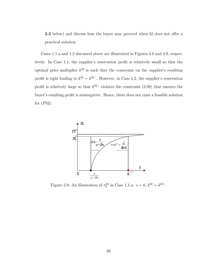
2.3 below) and discuss how the buyer may proceed when b2 does not offer a
practical solution.
Cases 1.1.a and 1.2 discussed above are illustrated in Figures 3.8 and 3.9, respec-
tively. In Case 1.1, the supplier’s reservation profit is relatively small so that the
optimal price multiplier kb2 is such that the constraint on the supplier’s resulting
profit is tight leading to kb2 = kb2−. However, in Case 1.2, the supplier’s reservation
profit is relatively large so that kb2− violates the constraint (3.98) that ensures the
buyer’s resulting profit is nonnegative. Hence, there does not exist a feasible solution
for (Pb2).
kb −2
0
π b
k
Π 2b
πba
s
bkk4
2
2−
− =≤
π 2b
b
bca
ak
2−≥
bca
a
2−
Figure 3.8: An illustration of πb2b in Case 1.1.a: s = 0, kb2 = kb2−.
66

kb −20
π b
k
Π 2b
πba
s
bkk4
2
2−
− =≤bca
ak
2−≥
bca
a
2−
Figure 3.9: An illustration of πb in Case 1.2: s = 0, infeasible setting.
Recalling (3.42), (3.43), (3.44), (3.50), and (3.95) and using (3.97), the corre-
sponding wholesale price, retail price, order quantity, supplier’s, buyer’s,
and system profits under the optimal b2 for s = 0 and π−s ∈ (0, (a2−2abc)/(4b)]
are given by
wb2 =2π−
s
a,
pb2 =a
2b,
qb2 =a
2,
πb2s = π−
s ,
πb2b =
a2
4b− ac
2− π−
s , and
Πb2 =a2
4b− ac
2.
For the case s = 0, if π−s ∈ (0, (a2 − 2abc)/(4b)] then either the setting (i.e. as in
Case 1.1.b) or the contract (i.e., as in Case 1.2) is impractical.
67

Case 2: s > 0.
Recalling (3.94), it is easy to verify that
g(0) < 0 and limk→+∞g(k) = +∞,
as well as
dg(k)
dk= 6s2b2k2 − 2s(s+ 2c)b2k. (3.100)
It then follows that there are two stationary points k01 and k0
2 of g(k) such that k01 = 0
and 0 < k02 = (s + 2c)/(3s) < +∞. Function g(k) as defined in (3.94) is illustrated
in Figure 3.10, where k0 denotes the reflection point such that
d2g(k)
dk2= 12s2b2k − 2s(s+ 2c)b2 = 0 (3.101)
for k = k0. As we can see from Figure 3.94, g(k) has a unique positive root, denoted
by kb2+, such that
g(kb2+) = 0. (3.102)
s
csk
3
202
+=2a−
)(kg
k001 =k
+2bk
s
csk
620 +=
Figure 3.10: An illustration of g(k) in (3.94).
68

Let us verify if kb2+ is realizable over the region (3.49) which appears in (3.50). We
know from the development of (Pb2) that this verification is equivalent to ensuring
that πb in (3.50) is nonnegative for k = kb2+, i.e., it suffices to verify that
πb |k=kb2+ ≥ 0.
To this end,
• Recall that πb is concave (by (3.93)),
• Note that
dπb
dk
∣∣∣∣k= a
bs
= −s[a− b(s+ c)]
2≤ 0 (by (3.92) and assumption (3.5)), and
• Note that
πb
∣∣k= a
bs= 0 (by (3.50)).
Hence, πb is not only decreasing but also it reaches zero at k = a/(bs). It then follows
from the concavity of πb and the definition of kb2+i that πb ≥ 0 for kb2+ ≤ k ≤ a/(bs).
Hence, kb2+ is realizable over the region (3.49).
Substituting k = kb2+ in (3.51), the corresponding supplier’s profit is given by
πb2+s =
(a− bskb2+
)24bkb2+
. (3.103)
Next, we need to consider πb2+s given by (3.103) in relation to constraint (3.51)
in (Pb2).
• If πb2+s ≥ π−
s then (3.51) is satisfied for kb2+ so that the optimal price
ii.e., kb2+ is the unique positive stationary point of πb in (3.50).
69
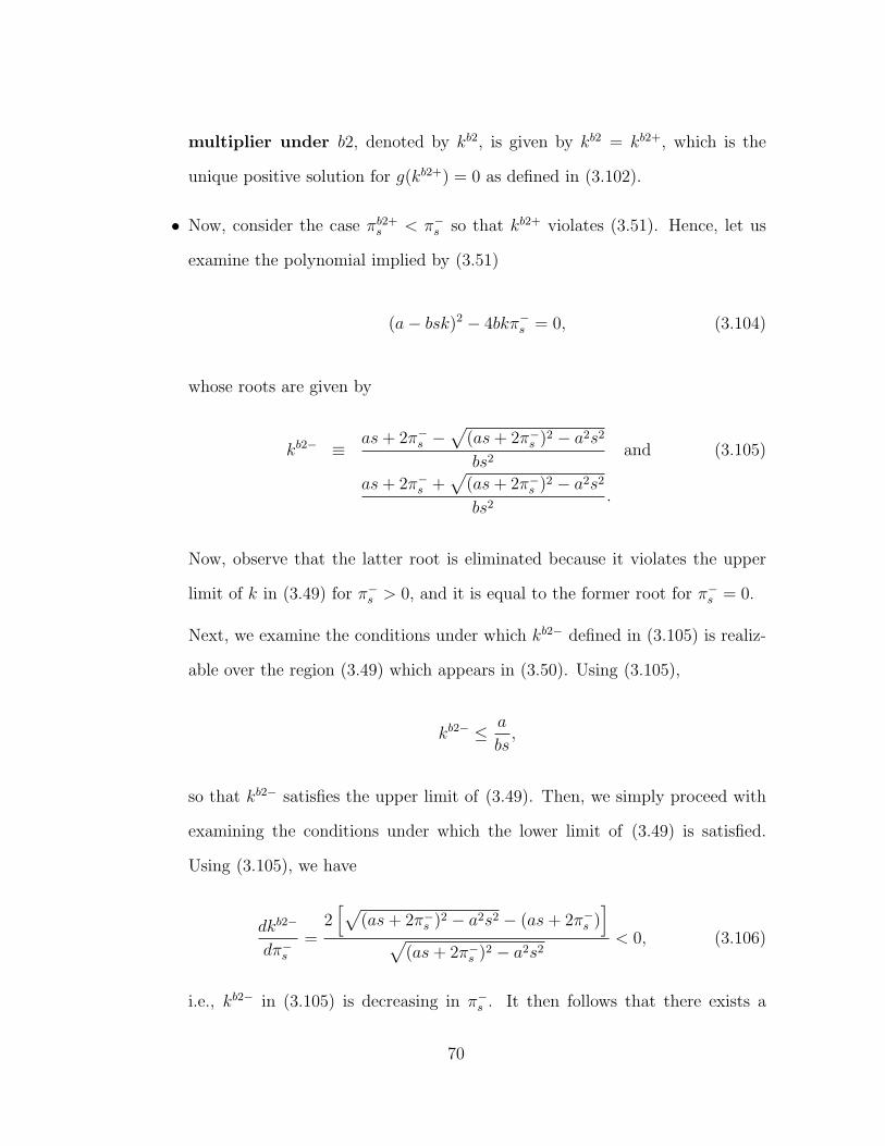
multiplier under b2, denoted by kb2, is given by kb2 = kb2+, which is the
unique positive solution for g(kb2+) = 0 as defined in (3.102).
• Now, consider the case πb2+s < π−
s so that kb2+ violates (3.51). Hence, let us
examine the polynomial implied by (3.51)
(a− bsk)2 − 4bkπ−s = 0, (3.104)
whose roots are given by
kb2− ≡as+ 2π−
s −√(as+ 2π−
s )2 − a2s2
bs2and (3.105)
as+ 2π−s +
√(as+ 2π−
s )2 − a2s2
bs2.
Now, observe that the latter root is eliminated because it violates the upper
limit of k in (3.49) for π−s > 0, and it is equal to the former root for π−
s = 0.
Next, we examine the conditions under which kb2− defined in (3.105) is realiz-
able over the region (3.49) which appears in (3.50). Using (3.105),
kb2− ≤ a
bs,
so that kb2− satisfies the upper limit of (3.49). Then, we simply proceed with
examining the conditions under which the lower limit of (3.49) is satisfied.
Using (3.105), we have
dkb2−
dπ−s
=2[√
(as+ 2π−s )
2 − a2s2 − (as+ 2π−s )]
√(as+ 2π−
s )2 − a2s2
< 0, (3.106)
i.e., kb2− in (3.105) is decreasing in π−s . It then follows that there exists a
70

threshold value of π−s such that if π−
s is greater than the threshold value then
kb2− ≤ kl. Letting πkls denote this threshold value and using (3.104) along with
(3.33),
πkls =
(a− bskl)2
4bkl≤ Πc, (3.107)
so that
– If π−s ∈ [0, πkl
s ] then kb2− ≥ kl and
– If π−s ∈ (πkl
s ,Πc] then kb2− < kl.
Hence, kb2− lies over the region (3.49) if π−s ∈ [0, πkl
s ]. Otherwise, if π−s ∈
(πkls ,Π
c], there does not exist a feasible solution for (PB2).
Using πs in (3.51), we have
dπs
dk=
−2bs(a− bsk)k − (a− bsk)2
4bk2= −(a− bsk)(a+ bsk)
4bk2. (3.108)
Hence, πs is decreasing in k over the region (3.49). That is,
• πs ≥ π−s only for those k such that k ≤ kb2−, and
• If πb2+s < π−
s then kb2− < kb2+.
Consequently, when π−s ∈ [0, πkl
s ], where πkls is defined in (3.107), recalling kb2+
defined in (3.102) and kb2− defined in (3.105),
kb2 = min{kb2−, kb2+} = min
{as+ 2π−
s −√
(as+ 2π−s )
2 − a2s2
bs2, kb2+
}. (3.109)
Recalling (3.42), (3.43), (3.44), (3.50), and (3.51), the corresponding whole-
sale price, retail price, order quantity, supplier’s, buyer’s, and system
71

profits under the optimal b2 for s > 0 and π−s ∈ [0, πkl
s ] are given by
wb2 =a+ bskb2
2bkb2= max
s+
√(as+ 2π−
s )2 − a2s2 − 2π−
s
2(as+ 2π−
s −√(as+ 2π−
s )2 − a2s2
) , a+ bskb2+
2bkb2+
,
pb2 =a+ bskb2
2b= min
{2as+ 2π−
s −√
(as+ 2π−s )
2 − a2s2
2bs,a+ bskb2+
2b
}, (3.110)
qb2 =a− bskb2
2= max
{√(as+ 2π−
s )2 − a2s2 − 2π−
s
2s,a− bskb2+
2
},
πb2s =
(a− bskb2)2
4bkb2= max
{π−s ,
(a− bskb2+)2
4bkb2+
},
πb2b =
(a− bskb2)[a(kb2 − 1) + bkb2(skb2 − s− 2c)]
4bkb2, and
Πb2 =(a− bskb2){a+ b[skb2 − 2(s+ c)]}
4b.
Also, recalling (3.33), we have π−s ∈ [0,Πc] by assumption. Then, considering
(3.103), (3.109) and the conditions on π−s under which πb2−
b defined in (3.105) is
realizable, we conclude that the optimal solution of (Pb2) depends on the value of
π−s :
• Case 2.1: s > 0, kb2 = kb2+. If π−s ∈ [0, πb2+
s ] then kb2+ ≤ kb2− so that
kb2 = kb2+,
• Case 2.2: s > 0, kb2 = kb2−. If π−s ∈ [πb2+
s , πkls ] then kb2+ ≥ kb2− so that
kb2 = kb2−, and
• Case 2.3: s > 0, infeasible setting. If π−s ∈ (πkl
s ,Πc] then there does not
exist a feasible solution for (Pb2). As for Case 1.2 above, while this case also
makes practical sense (perhaps, due to high profit expectation), b2 does not
offer a feasible solution. Note that this issue does not arise under b1 which
offers a meaningful solution for the buyer for all π−s such that π−
s ∈ [0,Πc].
72

Hence, the buyer can turn to b1 when π−s is relatively large. However, there is
a clear need for the buyer to pursue a more general contract than b1 and b2. As
we will show in the next section, the more general form of the generic contract
b3 does not only provide a practical solution but also it allows the buyer to
obtain more profit for π−s ∈ [0,Πc].
The three cases discussed above are illustrated in Figures 3.11, 3.12, and 3.13
respectively. In Case 1, the supplier’s reservation profit is relatively small so that
the unconstrained maximizer kb2+ of the buyer’s profit satisfies the constraint on the
supplier’s resulting profit. Hence, the optimal price multiplier kb2 is such that the
constraint is not binding leading to kb2 = kb2+. In Case 2, the buyer’s reservation
profit is relatively large so that kb2+ violates the constraint. Hence, the optimal price
multiplier is dictated by the binding constraint so that kb2 = kb2−. However, in Case,
the supplier’s reservation profit is very high, unlike b1 under which (Pb1) always has
a feasible solution for π−s ∈ [0,Πc], under b2, (Pb2) does not have a feasible solution
for π−s ∈ (πkl
s ,Πc].
bs
a
kb +2k l kb −2
kbk −≤ 2π b
k
π 2b
b
Figure 3.11: An illustration of πb2b in Case 2.1: s > 0, kb2 = kb2+.
73
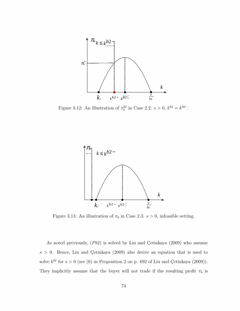
bs
a
kb +2k l kb −2
kbk −≤ 2π b
k
π 2b
b
Figure 3.12: An illustration of πb2b in Case 2.2: s > 0, kb2 = kb2−.
bs
akb +2k l k b −2
kbk −≤ 2π b
k
Figure 3.13: An illustration of πb in Case 2.3: s > 0, infeasible setting.
As noted previously, (Pb2) is solved by Liu and Cetinkaya (2009) who assume
s > 0. Hence, Liu and Cetinkaya (2009) also derive an equation that is used to
solve kb2 for s > 0 (see (6) in Proposition 2 on p. 692 of Liu and Cetinkaya (2009)).
They implicitly assume that the buyer will not trade if the resulting profit πb is
74

negative, while we provide the region of π−s that guarantees πb is nonnegative under
the optimal b2.
3.5.4 Optimal solution of (Pb3)
We believe that there is a clear need to examine the optimal b3 for three reasons:
• Contract b3, inspired by b1 and b2, proposes a more general pricing scheme.
• Contract b2 does not offer a practical solution for the buyer when the supplier’s
reservation profit is relatively high. We propose b3 in order to overcome this
issue while improving on the profit potential for the buyer (i.e., as another
alternative contract for the buyer).
• As we show momentarily, b3 is a coordination contract (see Cachon (2003)
and Tsay et al. (1999) for a formal discussion of coordination contracts). This
is because the total profit of the two entities is equal to the optimal centralized
system profit Πc so that profit potential of each party is in fact maximized
under b3. A coordination contract is said to achieve the so-called chan-
nel coordination objective (a phrase coined in the marketing literature as
indicated by Tsay et al. (1999)).
Recall (Pb3) given by (3.72) and (3.73). We present two approaches for deriving
the optimal solution of (Pb3). In the first approach, we examine the optimal solution
for the unconstrained problem associated with (Pb3) and then we incorporate
the main constraints (3.60) and (3.71) as well as the supplier’s reservation profit
constraint in (3.73). In the second approach, we establish an upper bound on the
objective function given by (3.72) and develop a feasible solution such that the ob-
jective function value of this solution achieves the upper bound. Hence, the feasible
solution at hand is also optimal.
75

Approach 1:
Using (3.72), for any given value of k > 0, observe that
∂πb
∂m=
a− b(km+m+ k2s− kc)
2kand (3.111)
∂2πb
∂m2= −b(k + 1)
2k< 0,
i.e., πb in (3.72) is concave in m for any k > 0. Letting m(k) denote the solution for
dπb/dm = 0 in (3.111), we have
m(k) =a+ b(kc− k2s)
b(k + 1). (3.112)
Substituting (3.112) in (3.71) and (3.60) and using assumption (3.5), it can be
easily verified that
[a+ b(sk −m(k))](k − 1)
2bk+m(k) =
a+ bc− bs
2b≥ c and
sk +m(k) = sk +a+ b(kc− k2s)
b(k + 1)=
a+ bk(s+ c)
b(k + 1)≤ a
b.
Hence, for any given k > 0, k and the corresponding m(k) in (3.112) satisfy the main
constraints (3.60) and (3.71) which appear in (Pb3).
Substituting (3.112) in (3.72), the buyer’s profit is given by
πb =k[a− b(s+ c)]2
4b(k + 1)=
[a− b(s+ c)]2
4b− [a− b(s+ c)]2
4b(k + 1), (3.113)
which is increasing over k > 0. Hence, the maximizer of πb in (3.113) is unbounded
76
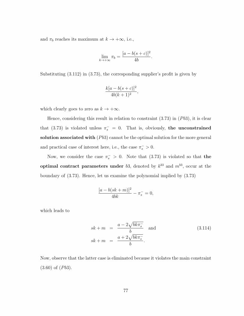
and πb reaches its maximum at k → +∞, i.e.,
limk→+∞
πb =[a− b(s+ c)]2
4b.
Substituting (3.112) in (3.73), the corresponding supplier’s profit is given by
k[a− b(s+ c)]2
4b(k + 1)2,
which clearly goes to zero as k → +∞.
Hence, considering this result in relation to constraint (3.73) in (Pb3), it is clear
that (3.73) is violated unless π−s = 0. That is, obviously, the unconstrained
solution associated with (Pb3) cannot be the optimal solution for the more general
and practical case of interest here, i.e., the case π−s > 0.
Now, we consider the case π−s > 0. Note that (3.73) is violated so that the
optimal contract parameters under b3, denoted by kb3 and mb3, occur at the
boundary of (3.73). Hence, let us examine the polynomial implied by (3.73)
[a− b(sk +m)]2
4bk− π−
s = 0,
which leads to
sk +m =a− 2
√bkπ−
s
band (3.114)
sk +m =a+ 2
√bkπ−
s
b.
Now, observe that the latter case is eliminated because it violates the main constraint
(3.60) of (Pb3).
77

Substituting (3.114) in (3.72), the buyer’s profit is given by
πb =
√bkπ−
s
[a−
√bkπ−
s − b(s+ c)]
b− π−
s . (3.115)
Then, we solve the optimal k that maximizes πb in the above equation. Letting
x =√bkπ−
s , πb in the above equation can be rewritten as a function of x such that
πb =x[a− x− b(s+ c)]
b− π−
s . (3.116)
It is equivalent for the buyer to solving the optimal x in (3.116) and solving the
optimal k in (3.115). Using (3.116), observe that
dπb
dx=
a− 2x− b(s+ c)
band
d2πb
dx2= −2
b< 0.
Hence, πb in (3.116) is concave and letting dπb/dx = 0 leads to x = [a− b(s+ c)]/2.
Substituting x = [a− b(s+ c)]/2 in√bkπ−
s = x and using (3.11) and (3.114), we
have
kb3 =[a− b(s+ c)]2
4bπ−s
=Πc
π−s
and (3.117)
mb3 = s+ c− s[a− b(s+ c)]2
4bπ−s
= c− s
(Πc
π−s
− 1
). (3.118)
Let us verify if kb3 and mb3 defined in (3.117) and (3.118) satisfy the main con-
straints (3.60) and (3.71) in (Pb3). We know from the development of (Pb3) that
this verification is equivalent to ensuring that πb in (3.72) is nonnegative for k = kb3
78
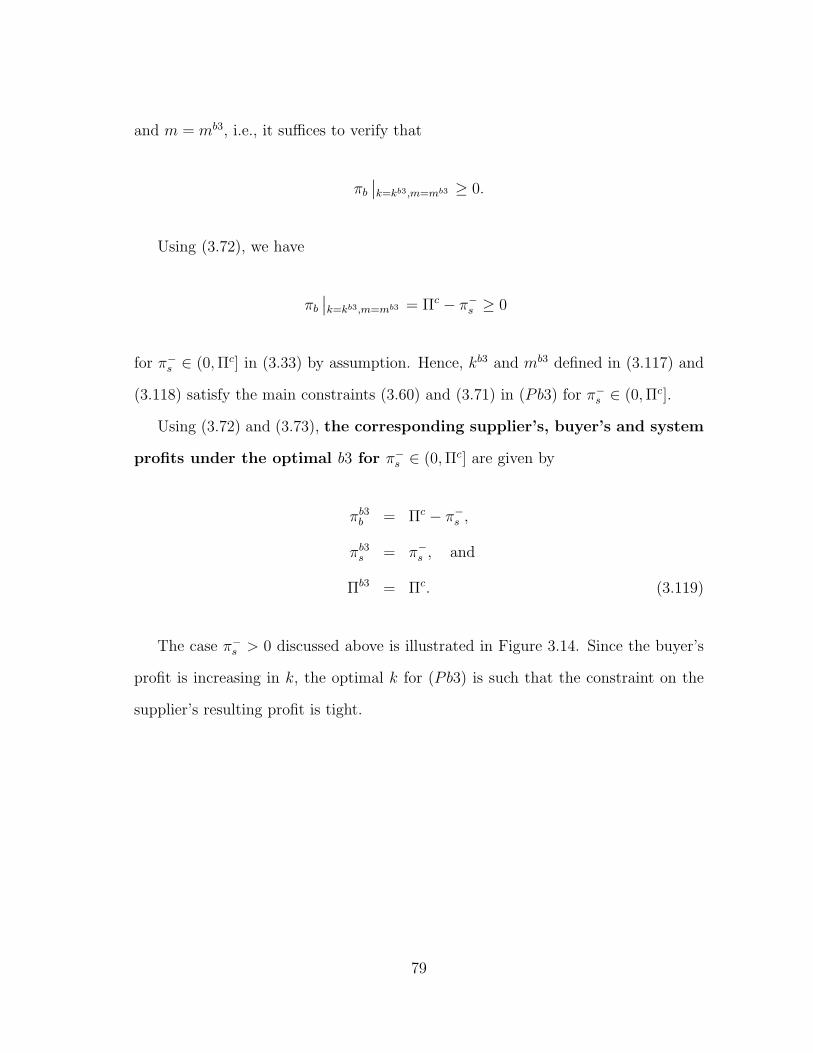
and m = mb3, i.e., it suffices to verify that
πb
∣∣k=kb3,m=mb3 ≥ 0.
Using (3.72), we have
πb
∣∣k=kb3,m=mb3 = Πc − π−
s ≥ 0
for π−s ∈ (0,Πc] in (3.33) by assumption. Hence, kb3 and mb3 defined in (3.117) and
(3.118) satisfy the main constraints (3.60) and (3.71) in (Pb3) for π−s ∈ (0,Πc].
Using (3.72) and (3.73), the corresponding supplier’s, buyer’s and system
profits under the optimal b3 for π−s ∈ (0,Πc] are given by
πb3b = Πc − π−
s ,
πb3s = π−
s , and
Πb3 = Πc. (3.119)
The case π−s > 0 discussed above is illustrated in Figure 3.14. Since the buyer’s
profit is increasing in k, the optimal k for (Pb3) is such that the constraint on the
supplier’s resulting profit is tight.
79
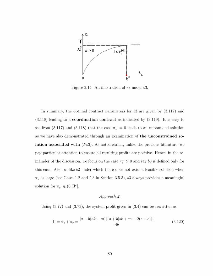
kb30
kbk 3≤
π b
k
Πc
0>kπ 3b
b
Figure 3.14: An illustration of πb under b3.
In summary, the optimal contract parameters for b3 are given by (3.117) and
(3.118) leading to a coordination contract as indicated by (3.119). It is easy to
see from (3.117) and (3.118) that the case π−s = 0 leads to an unbounded solution
as we have also demonstrated through an examination of the unconstrained so-
lution associated with (Pb3). As noted earlier, unlike the previous literature, we
pay particular attention to ensure all resulting profits are positive. Hence, in the re-
mainder of the discussion, we focus on the case π−s > 0 and say b3 is defined only for
this case. Also, unlike b2 under which there does not exist a feasible solution when
π−s is large (see Cases 1.2 and 2.3 in Section 3.5.3), b3 always provides a meaningful
solution for π−s ∈ (0,Πc].
Approach 2:
Using (3.72) and (3.73), the system profit given in (3.4) can be rewritten as
Π = πs + πb =[a− b(sk +m)]{a+ b[sk +m− 2(s+ c)]}
4b(3.120)
80

for k > 0 and m ∈ ℜ. Obviously, Π ≤ Πc always holds true, where Πc is the optimal
centralized system profit given in (3.11). Therefore, using (3.120), we observe that
πb = Π− πs =[a− b(sk +m)]{a+ b[sk +m− 2(s+ c)]}
4b− πs ≤ Πc − π−
s ,(3.121)
so that the best profit the buyer can achieve under b3 is given by Πc − π−s .
Next, we will provide a feasible solution of k and m such that πb = Πc − π−s is
true. Then, the feasible solution is also optimal under b3. Letting sk +m = x, the
system profit given in (3.120) can be written as
Π =(a− bx){a+ b[x− 2(s+ c)]}
4b, (3.122)
so that
dΠ
dx=
b(s+ c− x)
2and
d2Π
dx2= − b
2.
Hence, Π is concave in x. The maximizer of Π is given by x = s + c by solving
dΠ/dx = 0. It is easy to verify that Π = Πc at x = s+ c. Therefore, the equality in
(3.121) holds true if sk +m = s+ c and πs = π−s .
Next, we will show a feasible solution for k and m that satisfy these two equations
above. Substituting sk +m = s+ c in (3.73) and using (3.11), we have
πs =[a− b(sk +m)]2
4bk=
[a− b(s+ c)]2
4bk=
Πc
k. (3.123)
81

It can be easily verified that πs = π−s holds true if k = kb3, where
kb3 =Πc
π−s
, (3.124)
and sk +m = s+ c holds true if m = mb3, where
mb3 = s+ c− skb3 = c− s
(Πc
π−s
− 1
). (3.125)
Let us verify if kb3 and mb3 satisfy the main constraints (3.60) and (3.71) of
(Pb3). We know that the development of (Pb3) that this verification is equivalent
to ensuring that πb in (3.72) is nonnegative for k = kb3 and m = mb3. Recalling
πs = π−s and sk +m = s+ c for k = kb3 and m = mb3, we have
πb = Πc − π−s ≥ 0. (3.126)
It is because π−s ∈ [0,Πc] by assumption given by (3.33). Hence, kb3 and mb3 satisfy
the main constraints (3.60) and (3.71) of (Pb3). Since kb3 and mb3 are feasible, they
are also optimal as noted earlier.
Therefore, the optimal contract parameters under b3 are given by kb3 and
mb3 defined in (3.124) and (3.125), respectively. Using (3.67), (3.68), (3.69), (3.72),
and (3.73), the corresponding wholesale price, retail price, order quantity,
82

supplier’s, buyer’s and system profits under the optimal b3 are given by
wb3 =[a− b(s+ c)]π−
s
2bΠc+ s (3.127)
pb3 =a+ b(s+ c)
2b, (3.128)
qb3 =a− b(s+ c)
2,
πb3s = π−
s , (3.129)
πb3b = Πc − π−
s , and (3.130)
Πb3 = Πc. (3.131)
Last but not least, using (3.131), we reiterate that b3 is a coordination con-
tract. Hence, b3 is optimal from the system perspective.
3.6 Discussion and insights regarding b3
Now that we have developed the optimal contracts j under s1, b1, b2, and b3, we
provide a general discussion of these contracts while first emphasizing the advantages
of b3.
3.6.1 Advantages of b3 relative to b1, b2, b4, and b5
First, we note that while b3 has never been studied previously, two other coordi-
nation contracts have been investigated in the context of the buyer-driven channel
of interest here. These include the following two contracts:
b4. Under the buyer-driven two-part linear contract, the buyer decides the value of
k, k > 0, and the value of a lump-sum side payment, denoted by L, L ∈ ℜ,
while also committing that the retail price would be set such that p = kw and
the order quantity would be set such that q = a − bp = a − bkw. Next, the
jA summary of all formal results regarding these contracts is shown in Tables 3.2 and 3.3.
83

supplier decides w. Note that if L > 0 then a payment is transferred from
the supplier to the buyer, and if L < 0 then a payment is transferred from
the buyer to the supplier. This contract has been investigated by Liu and
Cetinkaya (2009) who demonstrate that b4 is a coordination contract for
the buyer-driven channel analyzed here.
b5. Under the buyer-driven revenue-sharing contract, the buyer proposes ϕ, ϕ ∈
[0, 1], and commits to share a portion (1 − ϕ) of the selling revenue with the
supplier. Next, in return the supplier commits to set a wholesale price lower
than the supplier’s unit cost, i.e., w = ϕs. This contract was studied by Pan
et al. (2010). In fact, it was inspired by Cachon and Lariviere (2005) who
illustrate some conditions under which it is a coordination contract.
Note that while b3 merely specifies a unit wholesale price, b4 and b5 involve both
a wholesale and a lump-sum side payment. Hence, we argue that b3 is a simpler,
yet, general, effective and practical contract:
• We say that b3 is simpler than b4 and b5 because of the following reason: In
a widely cited review paper, Cachon (2003) argues that “the contract designer
may actually prefer to offer a simple contract even if that contract does not
optimize the supply chain’s performance. A simple contract is particularly de-
sirable if the contract’s efficiency is high (the ratio of supply chain profit with
the contract to the supply chains optimal profit) and if the contract designer
captures the lions share of supply chain profit.” Under b3, once the optimal
contract parameters are computed and the contract is signed, the only trans-
action between the supplier and the buyer is based on the wholesale price. Also,
the contract’s efficiency under the optimal b3 is one. While more sophisticated
contracts, e.g., a contract with a side payment such as b4 or a revenue sharing
84

contract such as b5, are expected to offer increased flexibility for coordination,
b3 achieves channel coordination via a single transaction. We refer to Cor-
bett and Tang (1999) for a detailed discussion of progressively sophisticated
contracts.
• We say that b3 is more general than not only b1 and b2 but also b5 because of
two specific reasons:
– The formulation in (Pb3) is such that b3 is a generalization of both b1 and
b2, i.e., (Pb3) reduces to (Pb1) when k = 1 and to (Pb2) when m = 0.
– The idea of revenue sharing in a contractual setting is first introduced
by Cachon and Lariviere (2005) who treat ϕ as an external parameter.
They examine both the single-product setting of interest in Figure 3.1 and
the more general newsvendor setting while they ignore reservation profits.
They are able to prove that b5 is a coordination contract if the distribution
cost c is negligible, i.e., c = 0. Since their results do not immediately
extend to the case with explicit reservation profits and distribution cost
c, we demonstrate that b5 is not a coordination contract unless c = 0
(see Appendix A). Pan et al. (2010) analyze b5 explicitly in two different
settings with two products:
∗ One-supplier-two-buyer setting, and
∗ Two-supplier-one-buyer setting
with linear price-sensitive deterministic demand functions. They also ig-
nore reservation profits and assume that the distribution costs of the buy-
ers are negligible. Since b5 is not a coordination contract neither for the
problem settings analyzed by Pan et al. (2010) nor for our problem setting
85

with explicit reservation profits and distribution cost c, we argue that b3
is a more promising coordination contract amenable to generalization.
• We say that b3 is effective because of the following two reasons:
– Only if π−s = Πc, the optimal b3 is equivalent to optimal b1 (see footnote
k).
– Only if π−s = sΠc/(s+ c), the optimal b3 is equivalent to optimal b2 (see
footnote l).
That is, it is very unlikely for b1 or b2 to be optimal in general while the optimal
b3 is system optimal as it is a coordination contract. Hence, we argue that
b3 is an effective contract, and
• We say that b3 is practical because: b3 offers a practical solution for all realistic
levels of the supplier’s reservation profit while for example b2 may fail to do so
(see Cases 1.2 and 2.3 in Section 3.5.3).
Next, in Section 3.6.2, we also argue that b3 offers flexibility for negotiation
between the supplier and the buyer. That is, not only b3 beats s1, b1, and b2 in
terms of the system-wide profit and the buyer’s profit, b3 can be utilized to create an
environment for negotiation when the supplier is the dominant party. Last but not
least, in Section 3.6.4, we also prove that b3 benefits consumers in terms of generating
a low retail price.
kSuppose π−s = Πc. Using (3.86), the optimal m under b1 is given by mb1 = c. Using (3.124)
and (3.125), the optimal k and m under b3 are given by kb3 = 1 and mb3 = c. Recalling k = 1under b1, the optimal contracts under b1 and b3 are equivalent if π−
s = Πc.lSuppose π−
s = sΠc/(s + c). Using (3.109), it can be shown that the optimal k under b2 isgiven by kb2 = (s + c)/s. Using (3.124) and (3.125), the optimal k and m under b3 are given bykb3 = (s+ c)/s and mb3 = 0. Recalling m = 0 under b2, the optimal contracts under b2 and b3 areequivalent if π−
s = sΠc/(s+ c).
86

3.6.2 Conditions under which b3 is superior to s1 for the supplier
We next show that b3 is superior to s1 not only for the buyer but also for the
supplier under a specific condition on the supplier’s reservation profit. This specific
condition is an important finding we wish to elaborate on because Liu and Cetinkaya
(2009) argue that leadership is always beneficial for the lead in both supplier and
buyer-driven channels when reservation profits are assumed to be equal to zero.
We proceed with comparing s1 and b3 to identify the condition. First, observe
that b3 is superior to s1 for the supplier if the supplier has an opportunity to set
π−s ≥ πs1
s , where π−s ∈ [0,Πc] is the supplier’s reservation profit under b3 and πs1
s
is the supplier’s optimal profit under s1 given by (3.81). Using πs1s in (3.81) and
Figures 3.4 and 3.5 and considering Cases 1 and 2 discussed in Section 3.5.1, it is
easy to see that
• πs1s = Πc/2 if π−
b ∈ [0,Πc/4] and
• πs1s ≤ Πc/2 if π−
b ∈ [Πc/4,Πc].
It then follows that
πs1s ≤ Πc
2
for all π−b ∈ [0,Πc]. Then, if the supplier has an opportunity to set
Πc
2≤ π−
s ≤ Πc (3.132)
under b3, b3 is superior to s1 from the supplier’s perspective, too.
Next, observe that the buyer would hold on to b3 if
πb3b ≥ πs1
b (3.133)
87

for the given level of π−s in (3.132), where πs1
b here is given by (3.76) and it is the
buyer’s corresponding profit when the supplier achieves the maximum profit under
s1, i.e., πs1b = Πc/4. Clearly, for the given level of π−
s in (3.132), we have
πb3b = Πc − π−
s .
Then, using the above equation in (3.133) and combining (3.133) with (3.132), we
have
Πc
2≤ π−
s ≤ 3Πc
4, (3.134)
which ensures that b3 is superior to s1 for the supplier. That is, the maximum profit
the supplier can achieve under s1 is 3Πc/4. In particular,
• As a rational decision maker, the supplier should set π−s = 3Πc/4 under b3. In
this case, πb3b = Πc/4, and, hence, the buyer is indifferent between s1 and b3.
• If the supplier sets π−s = Πc/2 then πb3
b = Πc/2. In this case, the supplier is
indifferent between s1 and b3, while the buyer obtains the best profit among
all cases when the supplier agrees to switch from s1 to b3.
Now that we have established the condition in (3.134) under which b3 is superior
to s1 for the supplier, we question if b4 (i.e., the other buyer-driven coordination
contract) is ever superior to s1 perhaps under a condition similar to (3.134). We
do not raise this question for b5 because b5 is not a coordination contract for our
problem setting with explicit reservation profits and distribution cost c.
88
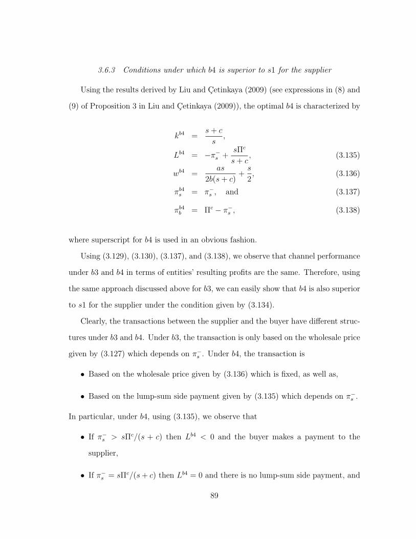
3.6.3 Conditions under which b4 is superior to s1 for the supplier
Using the results derived by Liu and Cetinkaya (2009) (see expressions in (8) and
(9) of Proposition 3 in Liu and Cetinkaya (2009)), the optimal b4 is characterized by
kb4 =s+ c
s,
Lb4 = −π−s +
sΠc
s+ c, (3.135)
wb4 =as
2b(s+ c)+
s
2, (3.136)
πb4s = π−
s , and (3.137)
πb4b = Πc − π−
s , (3.138)
where superscript for b4 is used in an obvious fashion.
Using (3.129), (3.130), (3.137), and (3.138), we observe that channel performance
under b3 and b4 in terms of entities’ resulting profits are the same. Therefore, using
the same approach discussed above for b3, we can easily show that b4 is also superior
to s1 for the supplier under the condition given by (3.134).
Clearly, the transactions between the supplier and the buyer have different struc-
tures under b3 and b4. Under b3, the transaction is only based on the wholesale price
given by (3.127) which depends on π−s . Under b4, the transaction is
• Based on the wholesale price given by (3.136) which is fixed, as well as,
• Based on the lump-sum side payment given by (3.135) which depends on π−s .
In particular, under b4, using (3.135), we observe that
• If π−s > sΠc/(s + c) then Lb4 < 0 and the buyer makes a payment to the
supplier,
• If π−s = sΠc/(s+ c) then Lb4 = 0 and there is no lump-sum side payment, and
89

• If π−s < sΠc/(s + c) then Lb4 > 0 and the supplier makes a payment to the
buyer.
3.6.4 Contract b3 is beneficial from consumers’ perspectives
We prove that b3 generates the lowest wholesale and retail prices among s1, b1,
b2, and b3, when π−s = π−
b = 0 and s > 0. Hence, b3 is beneficial from both buyer’s
and consumers’ perspectives in terms of the low prices. In particular, we show that
when π−s = π−
b = 0 and s > 0,
• wb3 ≤ wb2 ≤ wb1 ≤ ws1 and
• pb3 ≤ pb2 ≤ pb1 = ps1.
Since we do not have closed-form expressions for wb2 and pb2, we first prove that
• wb3 ≤ wb1 ≤ ws1 and
• pb3 ≤ pb1 = ps1.
Recalling (3.78) and (3.81), when π−b = 0, we have
ws1 =a+ b(s− c)
2band ps1 =
3a+ b(s+ c)
4b,
recalling (3.87) and (3.88), when π−s = 0, we have
wb1 =a+ b(3s− c)
4band pb1 =
3a+ b(s+ c)
4b,
and recalling (3.127) and (3.128), when π−s = 0, we have
wb3 = w and pb3 =a+ b(s+ c)
2b. (3.139)
90

Using the above equations, we have
ws1 − wb1 =a− b(s+ c)
4b≥ 0, wb1 − wb3 =
a− b(s+ c)
4b≥ 0,
ps1 − pb1 = 0, and pb1 − pb3 =a− b(s+ c)
4b≥ 0
using assumption (3.5). Hence we obtain
wb3 ≤ wb1 ≤ ws1 and pb3 ≤ pb1 = ps1. (3.140)
Next, we need to prove that
• wb3 ≤ wb2 ≤ wb1 and
• pb3 ≤ pb2 ≤ pb1.
To this end, recall (3.2) and note that the optimal wholesale price satisfies
dπs
dw=
[q + (w − s)
dq
dp
dp
dw
]= 0 (3.141)
under b1 and b2 according to (3.27) and (3.41), respectively. Note that under b1,
deciding on w is equivalent to deciding on p = w +m using (3.21) for the supplier
given m. Also, under b2, deciding on w is equivalent to deciding on p = kw using
(3.34) given k. Then, the optimal retail price satisfies
dπs
dp=
dw
dpq + (w − s)
dq
dp+ (w − s)
dq
dp= 0. (3.142)
1. Proof of wb3 ≤ wb2 ≤ wb1.
91

Under b1, p = w +m implies dp/dw = 1. Then, dπs/dw in (3.141) becomes
▽b1w =
[q + (w − s)
dq
dp
].
Under b2, p/w = k implies dp/dw = k ≥ 1 and dπs/dw in (3.141) becomes
▽b2w =
[q + k(w − s)
dq
dp
].
From ▽b1w and ▽b2
w we observe that the optimal wholesale price wb1 under b1
that satisfies ▽b1w = 0 would result in ▽b2
w ≤ 0, since k ≥ 1 and q ≥ 0 by
assumption. Recalling that πs is concave in w under b1 using (3.27) and under
b2 using (3.41), we have wb1 ≥ wb2. Also, ▽b2w = 0 implies wb2 ≥ s = wb3.
Then, we conclude wb3 ≤ wb2 ≤ wb1.
2. Proof of pb3 ≤ pb2 ≤ pb1.
Under b1, w = p−m implies dw/dp = 1 and dπs/dp in (3.142) becomes
▽b1p =
[q + (w − s)
dq
dp
].
Under b2, w/p = 1/k implies dw/dp = 1/k ≤ 1 and dπs/dp in (3.142) becomes
▽b2p =
[q
k+ (w − s)
dq
dp
].
From ▽b1p and ▽b2
p we observe that the optimal retail price pb1 under b1 that
satisfies ▽b1p = 0 would result in ▽b2
p ≤ 0, since k ≥ 1 and q ≥ 0 by assumption.
Hence, pb2 ≤ pb1.
Next, we need to show pb2 ≥ pb3. Using (3.110), when π−s = 0 and s > 0, we
92

have
pb2 =a+ bskb2
2b. (3.143)
In order to show pb2 ≥ pb3, using (3.139) and (3.143), we need to show that
kb2 ≥ (s + c)/s. Under b2, using (3.93), πb in (3.50) is concave in k and
kb2 satisfies the first-order condition of πb if π−s = 0 and s > 0. Note that
πb = Π − πs, where Π is the system profit. Using (3.50) and (3.51), under b2,
we have
Π =(a− bsk){a+ b[sk − 2(s+ c)]}
4band
dΠ
dk=
sb(s+ c− sk)
2⇒ dΠ
dk
∣∣∣∣k=(s+c)/s
= 0.
By (3.108), dπs/dk ≤ 0 at k = (s + c)/s by assumption (3.5). Therefore, we
have
dπb
dk
∣∣∣∣k=(s+c)/s
=dΠ
dk
∣∣∣∣k=(s+c)/s
− dπs
dk
∣∣∣∣k=(s+c)/s
≥ 0.
Due to the concavity of πb shown in (3.93), kb2 ≥ (s+c)/s. Therefore, pb2 ≥ pb3.
Then, we conclude pb3 ≤ pb2 ≤ pb1.
In summary, not only b3 beats s1, b1, and b2 in terms of the system-wide profit,
the buyer’s profit, and the supplier’s profit, it is also beneficial from the consumers’
perspectives. Also, the optimal wholesale and retail prices under buyer-driven con-
tracts, b1, b2, and b3, are not more than those under the supplier-driven contract
s1. The buyer-driven contracts regardless of contract type is more efficient than s1,
since they mitigate the double marginalization problem (Spengler (1950) and Tirole
(1988)) which raises the retail price and harms the system profit. The reason why the
buyer-driven channel is more efficient is explained by Liu and Cetinkaya (2009): “In
the supplier-driven channel, the buyer is the follower and responds to the suppliers
93

wholesale price. Since the supplier seeks to maximize the profit, the buyer is pushed
to select a higher than system optimal retail price which limits the market demand.
On the other hand, when the buyer is the leader, she selects the k value (determines
the quantity-price relation first) before the supplier declares the wholesale price, and
thus, the buyer has more freedom to warrant a higher market demand by choosing
a relatively smaller retail price which is closer to the system optimal retail price.”
3.7 Conclusion
In this chapter, we consider the basic bilateral monopolistic setting and propose
a new contract in the buyer-driven channel. The new contract referred as the generic
contract, b3, has a more general pricing scheme than the two existing buyer-driven
contracts in the literature: the margin-only and the multiplier-only contracts, i.e., b1
and b2. Considering the reservation profit for the supplier, we formulate the buyer’s
optimization problem (Pb3) under b3. We show that (Pb3) reduces to (Pb1) (the
problem under b1) when k = 1 and to (Pb2) (the problem under b2) when m = 0.
Examining (Pb1), (Pb2), and (Pb3), we study the optimal contracts under b1, b2,
and b3. Our work attempts to contribute the literature regarding the following:
• Contract b3 has never been studied previously;
• We incorporate the supplier’s reservation profit consideration under b1;
• We consider both cases s = 0 and s > 0 under b2 and provide the conditions
on the supplier’s reservation profit under which b2 is practical.
Finally, we provide an explicit comparison of the buyer- and supplier-driven chan-
nels by considering the wholesale price contract s1 in the supplier-driven channel,
and b1, b2, b3, as well as, existing coordination contracts in the buyer-driven channel:
the buyer-driven two-part linear contract, b4, and the buyer-driven revenue-sharing
94

contract, b5. We demonstrate that b3 is not only optimal for the system and the
buyer, it also benefits consumers and even the supplier. In summary,
• Contract b3 is a coordination contract and it is effective than b1 and b2.
• Contract b3 is more general than b1, b2, and b5.
• Contract b3 is simpler to implement than b4 and b5.
• Contract b3 is even superior to s1 for the supplier under a specific condition.
• Contract b3 benefits consumers by generating the lowest retail price among the
contracts of interest. It also solves the double marginalization problem.
95

Table 3.1: Summary of notation in the single-product setting.
Symbol Explanationp the retail priceq the order quantity, q = a− bpw the wholesale prices the supplier’s unit production cost, s ≥ 0c the buyer’s unit distribution cost, c ≥ 0k the price multiplier, k > 0m the price marginπs the supplier’s profit functionπb the buyer’s profit functionΠ the system profit function, Π = πs + πb
s1 index representing the wholesale price contract in the supplier-driven channelb1 index representing the margin-only contract in the buyer-driven channelb2 index representing the multiplier-only contract in the buyer-driven channelb3 index representing the generic contract in the buyer-driven channelΠc the centralized optimal system profitpc the centralized optimal retail priceqc the centralized optimal order quantity
ps1(w) the optimal retail price under s1 for a given wqs1(w) the optimal order quantity under s1 for a given wwb1(m) the optimal wholesale price under b1 for a given mpb1(m) the corresponding retail price under b1 for a given mqb1(m) the corresponding order quantity under b1 for a given mwb2(k) the optimal wholesale price under b2 for a given kpb2(k) the corresponding retail price under b2 for a given kqb2(k) the corresponding order quantity under b2 for a given k
wb3(k,m) the optimal wholesale price under b3 for given k and mpb3(k,m) the corresponding retail price under b3 for given k and mqb3(k,m) the corresponding order quantity under b3 for given k and m
kl the optimal k under contract l = b2, b3ml the optimal m under contract l = b1, b3wl the optimal wholesale price under contract l = s1, b1, b2, b3pl the optimal retail price under contract l = s1, b1, b2, b3πls the supplier’s profit under the optimal contract l = s1, b1, b2, b3
πlb the buyer’s profit under the optimal contract l = s1, b1, b2, b3
Πl the system profit under the optimal contract l = s1, b1, b2, b3π−s the supplier’s reservation profit, π−
s ≥ 0π−b the buyer’s reservation profit, π−
b ≥ 0
96

Table 3.2: Summary of results under s1 and b1 in the single-product setting.
Contract Decisions
Wholesale priceContract
(π−b ∈ [0,Πc])
ws1 = min{ws1−, ws1+} = min
{a−2
√bπ−
b
b− c, a+b(s−c)
2b
}ps1 = min
{a−√
bπ−b
b, 3a+b(s+c)
4b
}qs1 = max
{√bπ−
b ,a−b(s+c)
4
}πs1s =
[a−b(s+c)−2
√bπ−
b
]√bπ−
b
bif π−
b ∈ [Πc/4,Πc][a−b(s+c)]2
8bif π−
b ∈ [0,Πc/4]
πs1b = max
{π−b ,
[a−b(s+c)]2
16b
}Πs1 =
[a−b(s+c)−
√bπ−
b
]√bπ−
b
bif π−
b ∈ [Πc/4,Πc]3[a−b(s+c)]2
16bif π−
b ∈ [0,Πc/4]
Margin-onlyContract
(π−s ∈ [0,Πc])
mb1 = min{mb1−,mb1+} = min
{a−2
√bπ−
s
b− s, a−b(s−c)
2b
}wb1 = max
{s+
√π−s
b, a+b(3s−c)
4b
}pb1 = min
{a−√
bπ−s
b, 3a+b(s+c)
4b
}qb1 = max
{√bπ−
s ,a−b(s+c)
4
}πb1s = max
{π−s ,
[a−b(s+c)]2
16b
}πb1b =
[a−b(s+c)−2
√bπ−
s
]√bπ−
s
bif π−
s ∈ [Πc/4,Πc][a−b(s+c)]2
8bif π−
b ∈ [0,Πc/4]
Πb1 =
[a−b(s+c)−
√bπ−
s
]√bπ−
s
bif π−
s ∈ [Πc/4,Πc]3[a−b(s+c)]2
16bif π−
b ∈ [0,Πc/4]
97

Table 3.3: Summary of results under b2 and b3 in the single-product setting.
Contract Decisions
Multiplier-onlyContract(s = 0,
π−s ∈ (0, a
2−2abc4b
])
kb2 = a2
4bπ−s
wb2 = 2π−s
a
pb2 = a2b
πb2s = π−
s
πb2b = a2
4b− ac
2− π−
s
Πb2 = a2
4b− ac
2
Multiplier-onlyContract(s > 0,
π−s ∈ [0, πkl
s ])
kb2 = min{kb2−, kb2+}
kb2− =as+2π−
s −√
(as+2π−s )2−a2s2
bs2
2s2b2{kb2+}3 − s(s+ 2c)b2{kb2+}2 − a2 = 0
wb2 = max
{s+
√(as+2π−
s )2−a2s2−2π−s
2(as+2π−
s −√
(as+2π−s )2−a2s2
) , a+bskb2+
2bkb2+
}pb2 = min
{2as+2π−
s −√
(as+2π−s )2−a2s2
2bs, a+bskb2+
2b
}qb2 = max
{√(as+2π−
s )2−a2s2−2π−s
2s, a−bskb2+
2
}πb2s = max
{π−s ,
(a−bskb2+)2
4bkb2+
}πb2b = (a−bskb2)[a(kb2−1)+bkb2(skb2−s−2c)]
4bkb2
Πb2 = (a−bskb2){a+b[skb2−2(s+c)]}4b
GenericContract
(π−s ∈ (0,Πc])
kb3 = Πc
π−s
mb3 = c− s(
Πc
π−s− 1)
wb3 = [a−b(s+c)]π−s
2bΠc + s
pb3 = a+b(s+c)2b
qb3 = a−b(s+c)2
πb3s = π−
s
πb3b = Πc − π−
s
Πb3 = Πc
98

4. THE GENERIC CONTRACT IN THE CASE OF MULTIPLE PRODUCTS
4.1 Setting 2. The multi-product bilateral monopolistic setting
We extend the basic bilateral monopolistic setting (the single-product set-
ting) by considering the more general multi-product bilateral monopolistic set-
ting referred as the two-product setting in Figure 4.1. Suppose that the two products
are substitutable. The supplier’s decisions pertain to the wholesale prices w1 and
w2, and the buyer’s decisions pertain to the order quantities q1 and q2 and the retail
prices p1 and p2. The order quantities are dictated by the general demand function
that depends linearly on the retail prices following
q1
q2
=
a1
a2
−
α1 −β1
−β2 α2
p1
p2
. (4.1)
Price competition occurs between the two substitutable products and it results
from cross-price effects (Ingene and Parry (2004)), i.e., each product’s demand de-
pends on both products’ retail prices. The demand function in (4.1) is the generalized
”linear demand function with cross-price effects” (e.g., Pashigian (1961), Ingene and
Parry (1995), Tyagi (2005), and Yang and Zhou (2006)). In (4.1), ai, αi, and βi are
parameters, i = 1, 2. Parameter ai can be considered as the maximum demand of
product i in market when prices for both products are zero (McGuire and Staelin
(1983)). Parameter αi represents the sensitivity of demand of product i to its own re-
tail price and βi represents the sensitivity of demand of product i to the substitutable
product’s retail price (Ingene and Parry (2004)), i = 1, 2.
Let si and ci denote the supplier’s unit production cost and the buyer’s unit
distribution cost, respectively, for product i, i = 1, 2. The notation introduced so far
99

and used frequently in the remainder of this document is summarized in Table 4.1.
BuyerSupplier
w1
w2
p1, q1 = a� - α�p1 + ��p2
p2, q2 = a� - α�p2 + β�p1
Figure 4.1: The multi-product bilateral monopolistic setting.
Table 4.1: Summary of notation in the multi-product setting.
Symbol Explanationi the index of a product, i = 1, 2pi the retail price for product iqi the order quantity for product i, qi = ai − αipi + βipj, j = 1, 2, j = iαi the sensitivity of demand of product i to piβi the sensitivity of demand of product i to pj, j = 1, 2 and j = iwi the wholesale price for product isi the supplier’s unit production cost for product ici the buyer’s unit distribution cost for product iki the price multiplier for product i, ki > 0mi the price margin for product i, mi ∈ ℜ
We focus on the examination of the wholesale price contract in the supplier-driven
channel and the generic contract in the buyer-driven channel, denoted by s1 and b3,
respectively:
s1. Under the wholesale price contract, the supplier decides w1 and w2 and then
the buyer decides p1 and p2.
b3. Under the generic contract, the buyer decides on the values of ki, ki ∈ ℜ and
mi, mi ∈ ℜ, while also committing that the retail price for product i would be
100

set such that pi = kiwi +mi and the order quantity for product i would be set
such that qi = ai − αi(kiwi +mi) + βi(kjwj +mj), i, j = 1, 2 and j = i. Next,
the supplier decides wi, i = 1, 2.
4.2 Modeling the case of symmetric two products
We start the analysis by considering the so-called symmetric setting (Choi (1991))
for the two products. In the symmetric setting, ai = a, αi = α, βi = β, si = s, and
ci = c, i = 1, 2. Then, the demand function in (4.1) for product i can be rewritten
as
qi = a− αpi + βpj, (4.2)
i, j = 1, 2 and j = i. Hence, (4.2) is known as the “symmetric linear demand function
with cross-price effects”, which is the special case of the generalized “linear demand
function with cross-price effects” as shown in (4.1). The symmetry assumption for
products’ demands as applied in (4.2) has been widely adopted in the literature on
channel management to keep the problem formulation simple (e.g., McGuire and
Staelin (1983), Choi (1991), Choi (1996), Trivedi (1998), Pan et al. (2010), and Wu
et al. (2012)).
Due to the nature of price competition between substitutable products, α > 0
and β ≥ 0 are required, i.e., each product’s demand decreases in its own price and
increases in its competitor’s price. Assuming a product’s demand impacted by its
own price more heavily than by its competitor’s price, we set α > β (e.g., McGuire
and Staelin (1983), Choi (1991), Choi (1996), Trivedi (1998), Pan et al. (2010), and
Wu et al. (2012)). Hence, we assume α and β such that
α > β ≥ 0. (4.3)
101

In the following, we first examine the symmetric two-product setting. Next, we
generalize the symmetric two-product setting to the symmetric n-product setting,
n ≥ 2, and the asymmetric two-product setting. We analyze b3 in these two settings
in Sections 4.3 and 4.5. We conclude by summarizing the relations of these settings
to the single-product setting in Section 4.4.
4.2.1 Profit functions
In the symmetric two-product setting, using (4.2), the supplier’s profit function
is given by
πs =∑i=1,2
(wi − s)qi =∑
i,j=1,2,j =i
(wi − s)(a− αpi + βpj). (4.4)
The buyer’s profit function is given by
πb =∑i=1,2
(pi − wi − c)qi =∑
i,j=1,2,j =i
(pi − wi − c)(a− αpi + βpj). (4.5)
The centralized profit function is given by
Π =∑i=1,2
(pi − s− c)qi =∑
i,j=1,2,j =i
(pi − s− c)(a− αpi + βpj). (4.6)
Note that using (4.2), pi can be written as a function of order quantities such that
pi =a
α− β− αqi
α2 − β2− βqj
α2 − β2, (4.7)
i, j = 1, 2 and j = i.
Recalling (4.4), (4.5), (4.6), and (4.7), in order to guarantee qi ≥ 0 and the
supplier’s and buyer’s profits on product i are nonnegative, we assume pi ≤ a/(α−
102

β), wi ≥ s, and pi ≥ wi + c so that
s+ c ≤ wi + c ≤ pi ≤a
α− β, (4.8)
i = 1, 2. We pay particular attention to ensure that the contractual problems at
hand lead to nonnegative profits πs, πb, and Π for the sake of practical realism. The
inequalities in (4.8) are proposed to guarantee the nonnegative profits.
4.2.2 Centralized problem
Using (4.6) and assumption (4.8), the centralized optimization problem in the
symmetric two-product setting can be stated as
(Pc− 2s) : maxp1,p2∈[s+c,a/(α−β)]
Π =∑
i,j=1,2,j =i
(pi − s− c)(a− αpi + βpj).
Clearly, wi is immaterial for Π in (4.6), and, hence, by assumption (4.8), we are only
interested in pi values that satisfy
s+ c ≤ pi ≤a
α− β, (4.9)
i = 1, 2.
Using (4.6), note that
∂Π
∂pi= a− 2αpi + 2βpj + (α− β)(s+ c), (4.10)
i, j = 1, 2 and j = i, and the Hessian matrix of Π is given by
∂2Π∂p21
∂2Π∂p1∂p2
∂2Π∂p2∂p1
∂2Π∂p22
=
−2α 2β
2β −2α
.
103

The determinant of the Hessian matrix is given by 4α2−4β2 > 0 using (4.3). Hence,
Π in (4.6) is negative-definite. Setting ∂Π/∂pi = 0 in (4.10) for i = 1, 2 leads to
pci =a+ (α− β)(s+ c)
2(α− β). (4.11)
Observe that pci defined in (4.11) is the centralized optimal retail price for
product i, i = 1, 2. This is because by assumption (4.8),
a
α− β− pci =
a− (α− β)(s+ c)
2(α− β)≥ 0 and
pci − (s+ c) =a− (α− β)(s+ c)
2(α− β)≥ 0,
so that pci defined in (4.11) is realizable over the region (4.9), i = 1, 2. Using (4.11)
in (4.2), the centralized optimal order quantity for product i is given by
qci =a− (α− β)(s+ c)
2, (4.12)
i = 1, 2. Substituting (4.11) in (4.6), the centralized optimal system profit is
given by
Πc =[a− (α− β)(s+ c)]2
2(α− β). (4.13)
It is important to note that the optimal retail prices and order quantities given
by (4.11) and (4.12) for both products are the same, i.e., free of the index i, i = 1, 2.
It is because the two products are symmetric and it does not make sense to make
different decisions for them.
Ingene and Parry (2004) consider a variant of (Pc−2s) by allowing a more general
cost structure where each entity has a per unit cost as well as a fixed cost for each
product and using a more general demand function where a1 = a2 is possible. By
104

setting the fixed costs equal zero and letting a1 = a2, their problem (see the problem
in (5.3.1) on p. 199 of Ingene and Parry (2004)) is reduced to (Pc − 2s) leading to
pc in (4.11) (see (5.3.2) on p. 199 of Ingene and Parry (2004)).
4.2.3 Wholesale price contract s1
Under s1, the supplier decides w1 and w2 first and then the buyer decides p1 and
p2. By assumption (4.8), we are only interested in wi and pi values that satisfy
s ≤ wi ≤a
α− β− c and (4.14)
wi + c ≤ pi ≤a
α− β, (4.15)
i = 1, 2. We refer to (4.14) as the main constraint on the decision variables of the
contract design problem under s1.
4.2.3.1 Formulation of (Ps1− 2s)
For a given wi, i = 1, 2, such that (4.14) is true, using (4.5), we have
∂πb
∂pi= a− 2αpi + 2βpj + αwi − βwj + (α− β)c, (4.16)
i, j = 1, 2 and j = i, and the Hessian matrix of πb in (4.5) is given by
∂2πb
∂p21
∂2πb
∂p1∂p2
∂2πb
∂p2∂p1
∂2πb
∂p22
=
−2α 2β
2β −2α
.
The determinant of the Hessian matrix is given by 4α2−4β2 > 0 using (4.3). Hence,
πb in (4.5) is negative-definite. Setting ∂πb/∂pi = 0 in (4.16) for i = 1, 2 leads to
ps1−2si (wi) =
a+ (α− β)(wi + c)
2(α− β). (4.17)
105

Observe that for any wi such that (4.14) is true, ps1−2si (wi) defined in (4.17) is
the buyer’s optimal response, i.e., the optimal retail price for product i,
i = 1, 2. This is because wi satisfies (4.14) so that
a
α− β− ps1−2s
i (wi) =a− (α− β)(wi + c)
2(α− β)≥ 0 and
ps1−2si (wi)− (wi + c) =
a− (α− β)(w + c)
2(α− β)≥ 0,
i = 1, 2. Hence, ps1−2si (wi) in (4.17) is realizable over the region (4.15), i = 1, 2.
Using (4.2), the buyer’s optimal order quantity for product i is given by
qs1−2si (wi, wj) =
a− αwi + βwj − (α− β)c
2, (4.18)
i, j = 1, 2 and j = i.
Using (4.17) in (4.4) and (4.5), we have
πs =∑
i,j=1,2,j =i
(wi − s)[a− αwi + βwj − (α− β)c]
2and
πb =∑
i,j=1,2,j =i
[a− (α− β)(wi + c)][a− αwi + βwj − (α− β)c]
4(α− β).
Considering the main constraint (4.14) and the buyer’s reservation profit π−b
and using the two above expressions for πs and πb, the supplier’s optimization
106

problem under s1 in the symmetric two-product setting can be stated as
(Ps1− 2s) :
maxs≤w1,w2≤a/(α−β)−c
πs =∑
i,j=1,2,j =i
(wi − s)[a− αwi + βwj − (α− β)c]
2(4.19)
s.t. πb =∑
i,j=1,2,j =i
[a− (α− β)(wi + c)][a− αwi + βwj − (α− β)c]
4(α− β)
≥ π−b . (4.20)
Clearly, (Ps1 − 2s) makes sense only for reasonable values of π−b . That is, a
natural upper bound on π−b is given by
0 ≤ π−b ≤ Πc =
[a− (α− β)(s+ c)]2
2(α− β), (4.21)
where Πc is the optimal centralized system profit in (4.13).
It is important to note that a variant of (Ps1− 2s) is studied by Yang and Zhou
(2006). They consider a channel where a supplier sells a single product with cross-
price effects to two buyers who collude to make retail price decisions. The supplier’s
problem in their work can be considered as a variant of (Ps1−2s), where the supplier
makes only one wholesale price decision. Also, they assume π−b = 0 and c = 0 (see
Section 3.2 on p. 108 of Yang and Zhou (2006)). That is, setting w1 = w2 = w, πb in
(4.20) and ps1−2si (wi) in (4.17) also appear in their work (see expressions (11), (12),
and (13) on p. 108 of Yang and Zhou (2006)) with c = 0, i = 1, 2 .
4.2.3.2 Optimal solution of (Ps1− 2s)
Next, we present two approaches to identify the optimal solution for (Ps1− 2s)
given by (4.19) and (4.20). In the first approach, we prove that the optimal solution is
the same as that for (Ps1−2s) in the single-product setting. In the second approach,
107

we apply the method of Lagrange Multiplier to directly solve this problem.
Approach 1
Using (4.19), we have
πs =1
2
∑i=1,2
{(wi − s)[a− αwi − (α− β)c]− βswi}+ βw1w2. (4.22)
Note that
2w1w2 ≤ w21 + w2
2 (4.23)
for w1, w2 ∈ ℜ, where the equality holds true if w1 = w2. Using (4.22), we have
πs ≤ 1
2
∑i=1,2
{(wi − s)[a− αwi − (α− β)c]− βswi}+β
2(w2
1 + w22)
=∑i=1,2
(wi − s)[a− (α− β)(wi + c)]
2=∑i=1,2
f(wi), (4.24)
where the equality holds true if w1 = w2 and
f(x) =(x− s)[a− (α− β)(x+ c)]
2. (4.25)
108

Using (4.20) and (4.23), we have
πb =1
4(α− β)·∑
i=1,2
{[a− (α− β)(wi + c)][a− αwi − (α− β)c] + [a− (α− β)c]βwi}
−(α− β)βw1w2
2(α− β)
≥ 1
4(α− β)·∑
i=1,2
{[a− (α− β)(wi + c)][a− αwi − (α− β)c] + [a− (α− β)c]βwi}
−(α− β)β(w21 + w2
2)
4(α− β)
=∑i=1,2
[a− (α− β)(wi + c)]2
4(α− β)=∑i=1,2
g(wi), (4.26)
where the equality holds true if w1 = w2 and
g(x) =[a− (α− β)(x+ c)]2
4(α− β). (4.27)
Clearly, if
g(wi) ≥ π−b /2
for i = 1, 2 then using (4.26)
πb ≥∑i=1,2
g(wi) ≥ π−b .
Recalling (4.24), we have
πs ≤∑i=1,2
f(wi) ≤ maxw1,w2
∑i=1,2
f(wi) =∑i=1,2
maxwi
f(wi), (4.28)
109

where πs =∑
i=1,2 f(wi) if w1 = w2. Hence, the upper bound of πs in (4.19) when
πb ≥ π−b is satisfied is given by
∑i=1,2
maxwi
f(wi)
s.t. g(wi) ≥π−b
2, i = 1, 2.
Let w∗i denote the optimal solution to the above optimization problem, i = 1, 2.
Since this problem is separable based on wi, we have w∗i = w∗, i = 1, 2, where w∗ is
the optimal solution to the following optimization problem
maxw
f(w) =(w − s)[a− (α− β)(w + c)]
2
s.t. g(w) =[a− (α− β)(w + c)]2
4(α− β)≥ π−
b
2,
using (4.25) and (4.27). It is important to note that this optimization problem is
the same as (Ps1) in the single-product setting, when b = α− β and the buyer’s
reservation profit is given by π−b /2, where π−
b is the buyer’s reservation profit in the
symmetric two-product setting.
Since w1 = w2 = w∗, using (4.28), πs = f(w∗) + f(w∗) =∑
i=1,2maxwif(wi) =
2maxw f(w). In this case, πs achieves its upper bound. Hence, the optimal whole-
sale price for product i under s1 in the symmetric two-product setting is given by
ws1−2si = w∗, i = 1, 2, where w∗ is the optimal solution to (Ps1) in the single-product
setting with b = α− β and the buyer’s reservation profit is given by π−b /2.
110

Approach 2
Using (4.19), observe that
∂πs
∂wi
=(a− 2αwi + 2βwj + (α− β)(s− c))
2, (4.29)
i, j = 1, 2 and j = i, and the Hessian matrix of πs in (4.19) is given by
∂2πs
∂w21
∂2πs
∂w1∂w2
∂2πs
∂w2∂w1
∂2πs
∂w22
=
−α β
β −α
.
Hence, the Hessian matrix is negative-definite using (4.3). Letting ws1+i denote the
solution for ∂πs/∂wi = 0 in (4.29), we have
ws1+i = ws1+ ≡ a+ (α− β)(s− c)
2(α− β), (4.30)
i = 1, 2. Note that ws1+i is free of the index i, i = 1, 2. Hence, the subscript can be
omitted. Using assumption (4.8), it can be easily verified that ws1+i defined in (4.30)
is realizable over the region (4.14) which appears in (4.19), i = 1, 2. Substituting
(4.30) in (4.20), the corresponding buyer’s profit is the given by
πs1+b =
[a− (α− β)(s+ c)]2
8(α− β). (4.31)
Next, we need to consider πs1+b given by (4.31) in relation to constraint (4.20) in
(Ps1− 2s).
• If πs1+b ≥ π−
b then (4.20) is satisfied for wi = ws1+ so that the optimal
wholesale price for product i under s1, denoted by ws1−2si , is simply given
by ws1+ in (4.30), i = 1, 2.
111

• Otherwise, i.e., πs1+b < π−
b , ws1−2si occurs at the boundary of (4.20), i = 1, 2.
Then, we solve for ws1−2si using the method of Lagrange multiplier, i = 1, 2.
Let
f(·) = πs + λ(πb − π−b ),
where πs and πb are given by (4.19) and (4.20), λ ≥ 0 is the Lagrange multiplier,
and f(·) is a simplified notation for f(w1, w2, λ). Setting △wi,λf(·) = 0 leads
to
∂f(·)∂wi
=∂πs
∂wi
+λ∂πb
∂wi
=(1− λ)[a− (α− β)c] + (λ− 2)(αwi − βwj) + (α− β)s
2= 0,(4.32)
∂f(·)∂λ
= πb − π−b = 0, (4.33)
i, j = 1, 2 and j = i. Then, (4.32) leads to
wi =(λ− 1)[a− (α− β)c]− (α− β)s
(λ− 2)(α− β),
i = 1, 2. It is obvious that w1 = w2 by the above equation. Hence, ws1−2s1 =
ws1−2s2 and let ws1−2s
i = ws1−2s, i = 1, 2. Letting wi = w, i = 1, 2, in (4.20) and
(4.33), we have
[a− (α− β)(w + c)]2 − 2(α− β)π−b = 0.
Therefore, ws1−2s is dictated by the solution of the above polynomial. The root
of the polynomial are given by
ws1− =a−
√2(α− β)π−
b
α− β− c and
a+√2(α− β)π−
b
α− β− c. (4.34)
112
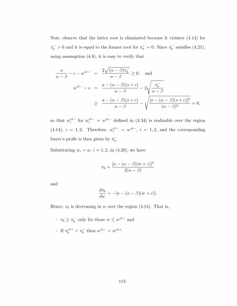
Now, observe that the latter root is eliminated because it violates (4.14) for
π−b > 0 and it is equal to the former root for π−
b = 0. Since π−b satisfies (4.21),
using assumption (4.8), it is easy to verify that
a
α− β− c− ws1− =
2√(α− β)π−
b
α− β≥ 0, and
ws1− − s =a− (α− β)(s+ c)
α− β− 2
√π−b
α− β
≥ a− (α− β)(s+ c)
α− β−
√[a− (α− β)(s+ c)]2
(α− β)2= 0,
so that ws1−i for ws1−
i = ws1− defined in (4.34) is realizable over the region
(4.14), i = 1, 2. Therefore, ws1−i = ws1−, i = 1, 2, and the corresponding
buyer’s profit is then given by π−b .
Substituting wi = w, i = 1, 2, in (4.20), we have
πb =[a− (α− β)(w + c)]2
2(α− β)
and
dπb
dw= −[a− (α− β)(w + c)].
Hence, πb is decreasing in w over the region (4.14). That is,
– πb ≥ π−b only for those w ≤ ws1− and
– If πs1+b < π−
b then ws1− < ws1+.
113

Consequently, recalling (4.30) and (4.34), we have
ws1−2si = min{ws1−, ws1+}
= min
{a−
√2(α− β)π−
b
α− β− c,
a+ (α− β)(s− c)
2(α− β)
}. (4.35)
Recalling (4.21), we have π−b ∈ [0,Πc] by assumption. Then, considering (4.31)
and (4.35), it is easy to show that the optimal solution of (Ps1− 2s) depends on the
value of π−b . That is,
• Case 1: ws1−2si = ws1+. If π−
b ∈ [0,Πc/4] then ws1+ ≤ ws1− so that ws1−2si =
ws1+, and
• Case 2: ws1−2si = ws1−. If π−
b ∈ [Πc/4,Πc] then ws1+ ≥ ws1− so that ws1−2si =
ws1−, i = 1, 2.
Recalling (4.17), (4.18), (4.19), and (4.20) and using (4.35), the corresponding
retail price, order quantity, supplier’s, buyer’s and system profits under
114

the optimal contract s1 are given by
ps1−2si = min
{2a−
√2(α− β)π−
b
2(α− β),3a+ (α− β)(s+ c)
4(α− β)
}, (4.36)
qs1−2si = max
{√(α− β)π−
b
2,a− (α− β)(s+ c)
4
},
πs1−2ss =
[a−(α−β)(s+c)−
√2(α−β)π−
b
]√2(α−β)π−
b
α−βif π−
b ∈ [Πc/4,Πc]
[a−(α−β)(s+c)]2
4(α−β)= Πc
2if π−
b ∈ [0,Πc/4]
, (4.37)
πs1−2sb = max
{π−b ,
[a− (α− β)(s+ c)]2
8(α− β)
}, and (4.38)
Πs1−2s =
[a−(α−β)(s+c)−
√(α−β)π−
b /2]√
2(α−β)π−b
α−βif π−
b ∈ [Πc/4,Πc]
3[a−(α−β)(s+c)]2
8(α−β)if π−
b ∈ [0,Πc/4]
.(4.39)
As noted previously, (Ps1− 2s) is solved by Yang and Zhou (2006) by assuming
π−b = 0 and c = 0 leading to the optimal wholesale price in (4.35), retail price in
(4.36), resulting profits in (4.37), (4.38), and (4.39) with π−b = 0 and c = 0 (see the
expressions in Table 1 on p. 110 of Yang and Zhou (2006)).
4.2.4 Generic contract b3
Under b3, the buyer announces that pi would be set depending on wi according
to
pi = kiwi +mi, (4.40)
where ki ∈ ℜ is the unconstrained multiplier and mi ∈ ℜ is the unconstrained value
representing a margin (mark-up) or rebate (mark-down), i = 1, 2. Then, the buyer
moves first and decides ki and mi and the supplier selects the optimal wi, i = 1, 2.
In the single-product setting, we show that if the unconstrained multiplier
for the single product is non-positive, i.e., k ≤ 0, then the buyer does not make any
115

profit. Hence, we restrict our attention to the case k > 0 under b3. It is natural
to argue the same result in the symmetric/assymetric two-product setting as well as
the symmetric n-product setting. Hence, we focus on ki > 0 under b3, i = 1, 2.
Substituting (4.40) in assumption (4.8), we have
s+ c ≤ wi + c ≤ pi = kiwi +mi ≤a
α− β,
i = 1, 2. Since wi ≥ s and ki > 0,
kis+mi ≤ kiwi +mi,
i = 1, 2. Hence, using the above inequalities, we conclude that ki, mi, wi, and pi
should be such that
kis+mi ≤a
α− β, (4.41)
s ≤ wi ≤a
α− β− c, and (4.42)
s+ c ≤ pi ≤a
α− β, (4.43)
i = 1, 2.
Let us examine πs in (4.4) under b3. For given ki > 0 and mi ∈ ℜ, i = 1, 2, using
(4.40), πs in (4.4) can be rewritten as
πs =∑
i,j=1,2,i =j
(wi − s)[a− αkiwi + βkjwj − (αmi − βmj)]. (4.44)
Note that
∂πs
∂wi
= a− 2αkiwi + β(ki + kj)wj + (α− β)kis− (αmi − βmj), (4.45)
116

i, j = 1, 2 and j = i, and the Hessian matrix of πs in (4.44) is given by
∂2πs
∂w21
∂2πs
∂w1∂w2
∂2πs
∂w2∂w1
∂2πs
∂w22
=
−2αk1 β(k1 + k2)
β(k1 + k2) −2αk2
.
The determinant of the Hessian matrix is given by
4α2k1k2 − β2(k1 + k2)2.
Here, we momentarily assume this quantity is greater than zero, and, hence, the
Hessian matrix is negative-definite. Later, we will show that under the optimal
contract the buyer would set k1 = k2, so that determinant of the Hessian matrix
reduces to
4(α2 − β2)k21 > 0,
since k1 > 0 by definition and (4.3).
Setting ∂πs/∂wi = 0 for i = 1, 2 in (4.45) leads to
wb3−2si (·) = [(kimi + kjmi − k2
j s− kjkis)β2 + (kjmj − kimj − kikjs+ k2
j s)αβ
+(2kikjs− 2mikj)α2 + (ki + kj)aβ + 2akjα] ·
1
4kikjα2 − (ki + kj)2β2, (4.46)
where wb3−2si (·) is a simplified notation for wb3−2s
i (k1,m1, k2,m2), i, j = 1, 2 and j = i.
Let us verify if wb3−2si (·) is realizable over the region (4.42), i = 1, 2. We know
from the development of (4.42) that this verification is equivalent to ensuring that
πs in (4.44) is nonnegative for wi = wb3−2si (·), i = 1, 2. Since wi = s, i = 1, 2, is
obviously a feasible solution under which πs = 0. Therefore, using the definition of
117

wb3−2si , πs ≥ 0 is true for wi = wb3−2s
i (·), i = 1, 2. Then, wb3−2si defined in (4.46) is the
supplier’s optimal response, i.e., the optimal wholesale price for product
i, under b3 because it is realizable over the region (4.42). Substituting (4.46) in
(4.40) and using (4.2), the corresponding retail price and order quantity for
product i for given values of ki > 0 and mi ∈ ℜ that satisfy (4.41) are given by
pb3−2si (·) = ki[(kimi + kjmi − k2
j s− kjkis)β2 + (kjmj − kimj − kikjs+ k2
j s)αβ
+(2kikjs− 2mikj)α2 + (ki + kj)aβ + 2akjα]/[4kikjα
2 − (ki + kj)2β2]
+mi and (4.47)
qb3−2si (·) = a− αpb3−2s
i (·) + βpb3−2sj (·), (4.48)
i, j = 1, 2 and j = i.
As noted in the single-product setting, (4.41), (4.42), and (4.43) are not sufficient
to guarantee πb ≥ 0 in (4.5). In order to guarantee πb ≥ 0, recalling assumption
(4.8) and using (4.46) and (4.47), we need to ensure
wb3−2si (·) + c ≤ pb3−2s
i (·), (4.49)
i = 1, 2. Hence, we refer to (4.41) and (4.49) as the main constraints for the problem
at hand.
Using (4.4) and (4.5), we have
πs =∑i=1,2
[wb3−2s
i (·)− s]qb3−2si (·) and
πb =∑i=1,2
[pb3−2si (·)− wb3−2s
i (·)− c]qb3−2si (·),
where wb3−2si (·), pb3−2s
i (·), and qb3−2si (·) are given by (4.46), (4.47), and (4.48), i = 1, 2.
118

Finally, considering (4.41), (4.49), the above expressions for πs and πb, and the
constraint ki > 0, the buyer’s optimization problem under b3 for the sym-
metric two-product setting can be stated as
(Pb3− 2s) : maxki>0,mi∈ℜ
πb =∑i=1,2
[pb3−2si (·)− wb3−2s
i (·)− c]qb3−2si (·) (4.50)
s.t. pb3−2si (·)− wb3−2s
i (·)− c ≥ 0
ski +mi ≤a
α− β
πs =∑i=1,2
[wb3−2s
i (·)− s]qb3−2si (·) ≥ π−
s , (4.51)
where wb3−2si (·), pb3−2s
i (·), and qb3−2si (·) are given by (4.46), (4.47), and (4.48), re-
spectively, i = 1, 2.
Clearly, (Pb3 − 2s) makes sense only for reasonable values of π−s . That is, a
natural upper bound on π−s is given by
0 ≤ π−s ≤ Πc =
[a− (α− β)(s+ c)]2
2(α− β), (4.52)
where Πc is the optimal centralized system profit in (4.13).
Next, we identify the optimal solution to (Pb3− 2s) given by (4.50) and (4.51).
To this end, we establish an upper bound on the objective function given by (4.50)
and develop a feasible solution such that the objective function value of this solution
achieves the upper bound. Hence, the feasible solution at hand is also optimal.
Using (4.50) and (4.51), the system profit under b3 is given by Π = πs + πb.
Obviously, Π ≤ Πc always holds true, where Πc is the optimal centralized system
profit given in (4.13). Therefore, under b3, we have
πb = Π− πs ≤ Πc − π−s ,
119
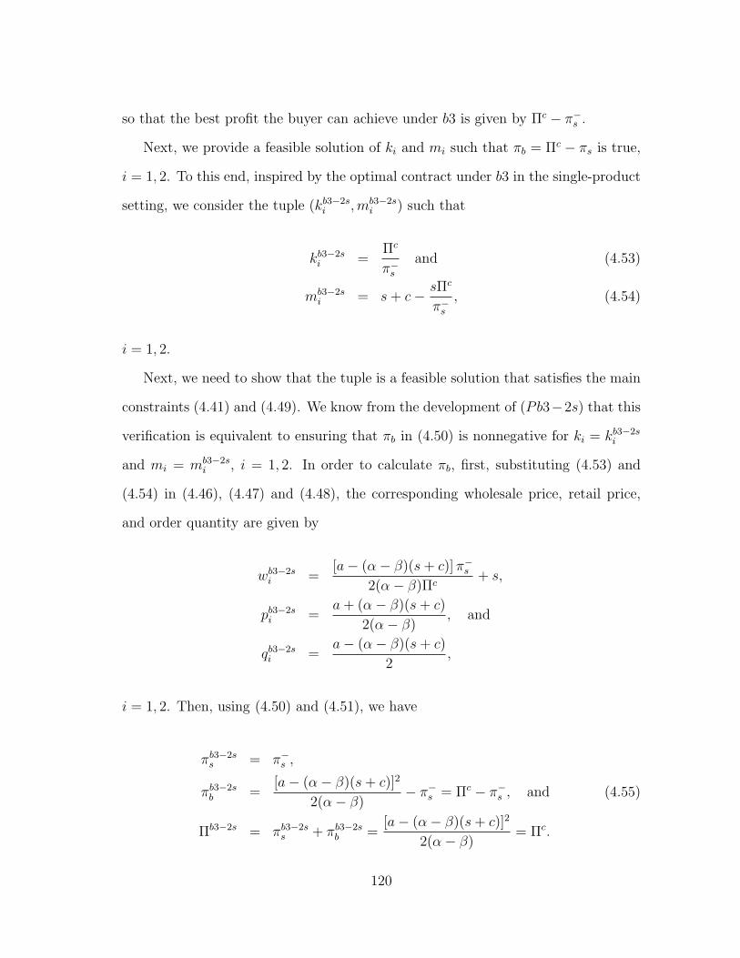
so that the best profit the buyer can achieve under b3 is given by Πc − π−s .
Next, we provide a feasible solution of ki and mi such that πb = Πc − πs is true,
i = 1, 2. To this end, inspired by the optimal contract under b3 in the single-product
setting, we consider the tuple (kb3−2si ,mb3−2s
i ) such that
kb3−2si =
Πc
π−s
and (4.53)
mb3−2si = s+ c− sΠc
π−s
, (4.54)
i = 1, 2.
Next, we need to show that the tuple is a feasible solution that satisfies the main
constraints (4.41) and (4.49). We know from the development of (Pb3−2s) that this
verification is equivalent to ensuring that πb in (4.50) is nonnegative for ki = kb3−2si
and mi = mb3−2si , i = 1, 2. In order to calculate πb, first, substituting (4.53) and
(4.54) in (4.46), (4.47) and (4.48), the corresponding wholesale price, retail price,
and order quantity are given by
wb3−2si =
[a− (α− β)(s+ c)] π−s
2(α− β)Πc+ s,
pb3−2si =
a+ (α− β)(s+ c)
2(α− β), and
qb3−2si =
a− (α− β)(s+ c)
2,
i = 1, 2. Then, using (4.50) and (4.51), we have
πb3−2ss = π−
s ,
πb3−2sb =
[a− (α− β)(s+ c)]2
2(α− β)− π−
s = Πc − π−s , and (4.55)
Πb3−2s = πb3−2ss + πb3−2s
b =[a− (α− β)(s+ c)]2
2(α− β)= Πc.
120

Using (4.55), it is easy to verify that πb3−2sb ≥ 0 since π−
s ≤ Πc in (4.52). Hence
the tuple (kb3−2si , mb3−2s
i ) defined in (4.53) and (4.54), i = 1, 2, is a feasible solution,
under which the upper bound of the objective function in (4.50) is achieved, i.e.,
πb = Πc − π−s . Hence, it is also optimal.
It is important to note that the optimal contract parameters given by (4.53)
and (4.54) for the two products are the same, i.e., free of the index i, i = 1, 2. It is
because the two products are symmetric and it does not make sense to make different
decisions for them.
4.3 Modeling the case of symmetric n products
Now that we have illustrated specific approaches simplifying the symmetric two-
product problems (Ps1−2s) and (Pb3−2s) in Section 4.2, we utilize the approaches
to derive the symmetric n-product problems (Ps1− ns) and (Pb3− ns), n ≥ 2.
In the symmetric n-product setting, we assume the order quantity for product i
is given by
qi = a− αpi +β
n− 1
∑j=1,··· ,n,j =i
pj, (4.56)
i = 1, · · · , n (Bresnahan and Reiss (1985)). Note that when n = 2, the demand
function in (4.56) is reduced to the demand function in (4.2) in the symmetric two-
product setting.
Profit functions:
In the symmetric n-product setting, the supplier’s profit function is given by
πs =∑
i=1,··· ,n
(wi − s)qi =∑
i=1,··· ,n
(wi − s)
(a− αpi +
β
n− 1
∑j=1,··· ,n,j =i
pj
). (4.57)
121
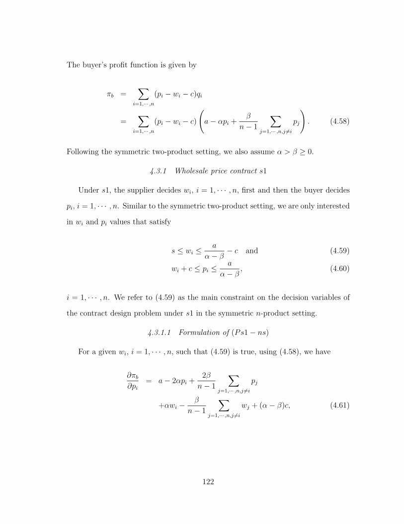
The buyer’s profit function is given by
πb =∑
i=1,··· ,n
(pi − wi − c)qi
=∑
i=1,··· ,n
(pi − wi − c)
(a− αpi +
β
n− 1
∑j=1,··· ,n,j =i
pj
). (4.58)
Following the symmetric two-product setting, we also assume α > β ≥ 0.
4.3.1 Wholesale price contract s1
Under s1, the supplier decides wi, i = 1, · · · , n, first and then the buyer decides
pi, i = 1, · · · , n. Similar to the symmetric two-product setting, we are only interested
in wi and pi values that satisfy
s ≤ wi ≤a
α− β− c and (4.59)
wi + c ≤ pi ≤a
α− β, (4.60)
i = 1, · · · , n. We refer to (4.59) as the main constraint on the decision variables of
the contract design problem under s1 in the symmetric n-product setting.
4.3.1.1 Formulation of (Ps1− ns)
For a given wi, i = 1, · · · , n, such that (4.59) is true, using (4.58), we have
∂πb
∂pi= a− 2αpi +
2β
n− 1
∑j=1,··· ,n,j =i
pj
+αwi −β
n− 1
∑j=1,··· ,n,j =i
wj + (α− β)c, (4.61)
122

i, j = 1, · · · , n and j = i, and the Hessian matrix of πb in (4.58) is given by
∂2πb
∂p21· · · ∂2πb
∂p1∂pn
.... . .
...
∂2πb
∂pn∂p1· · · ∂2πb
∂p2n
=
−2α · · · 2β
.... . .
...
2β · · · −2α
.
The determinant of the Hessian matrix is given by (2α)n− (2β)n > 0 by assumption.
Hence, πb in (4.58) is negative-definite. Setting ∂πb/∂pi = 0 in (4.61) for i = 1, · · · , n
leads to
ps1−nsi (wi) =
a+ (α− β)(wi + c)
2(α− β). (4.62)
Observe that for any wi such that (4.59) is true, ps1−nsi (wi) defined in (4.62) is
the buyer’s optimal response, i.e., the optimal retail price for product i,
i = 1, · · · , n. This is because wi satisfies (4.59) so that
a
α− β− ps1−ns
i (wi) =a− (α− β)(wi + c)
2(α− β)≥ 0 and
ps1−nsi (wi)− (wi + c) =
a− (α− β)(w + c)
2(α− β)≥ 0,
i = 1, · · · , n. Hence, ps1−nsi (wi) in (4.62) is realizable over the region (4.60), i =
1, · · · , n. Using (4.56), the buyer’s optimal order quantity for product i is
given by
qs1−nsi (w1, · · · , wn) =
a− αwi +β
n−1
∑j=1,··· ,n,j =iwj − (α− β)c
2, (4.63)
i, j = 1, · · · , n and j = i.
123

Using (4.62) in (4.57) and (4.58), we have
πs =∑
i=1,··· ,n
(wi − s)[a− αwi +β
n−1
∑j=1,··· ,n,j =i wj − (α− β)c]
2and
πb =∑
i=1,··· ,n
[a− (α− β)(wi + c)][a− αwi +β
n−1
∑j=1,··· ,n,j =i wj − (α− β)c]
4(α− β).
Considering the main constraint (4.59) and the buyer’s reservation profit π−b
and using the two above expressions for πs and πb, the supplier’s optimization
problem under s1 in the symmetric n-product setting can be stated as
(Ps1− ns) :
maxs≤wi≤a/(α−β)−c,i=1,··· ,n
πs =∑
i=1,··· ,n
(wi − s)[a− αwi +β
n−1
∑j=1,··· ,n,j =iwj − (α− β)c]
2(4.64)
s.t. πb =∑
i=1,··· ,n
[a− (α− β)(wi + c)][a− αwi +β
n−1
∑j=1,··· ,n,j =i wj − (α− β)c]
4(α− β)
≥ π−b . (4.65)
Clearly, (Ps1 − ns) makes sense only for reasonable values of π−b . That is, a
natural upper bound on π−b is given by
0 ≤ π−b ≤ Πc−n (4.66)
124

where Πc−n is the centralized optimal system profit, which can be calculated by
Πc−n = maxpi∈[s+c,a/(α−β)],i=1,··· ,n
Π
=∑
i=1,··· ,n
(pi − s− c)
(a− αpi +
β
n− 1
∑j=1,··· ,n,j =i
pj
). (4.67)
4.3.1.2 Optimal solution of (Ps1− ns)
Using (4.64), we have
πs =1
2
∑i=1,··· ,n
{(wi − s)[a− αwi − (α− β)c]− βswi +
β
n− 1wi
∑j=1,··· ,n,j =i
wj
}.
(4.68)
Note that
2wiwj ≤ w2i + w2
j (4.69)
for wi, wj ∈ ℜ, where the equality holds true if wi = wj, i, j = 1, · · · , n, i = j. Using
(4.68), we have
πs
≤ 1
2
∑i=1,··· ,n
{(wi − s)[a− αwi − (α− β)c]− βswi +
β
2w2
i +β
2(n− 1)
∑j=1,··· ,n,j =i
w2j
}
=∑
i=1,··· ,n
(wi − s)[a− (α− β)(wi + c)]
2=
∑i=1,··· ,n
f(wi), (4.70)
where the equality holds true if w1 = · · · = wn and
f(x) =(x− s)[a− (α− β)(x+ c)]
2. (4.71)
125
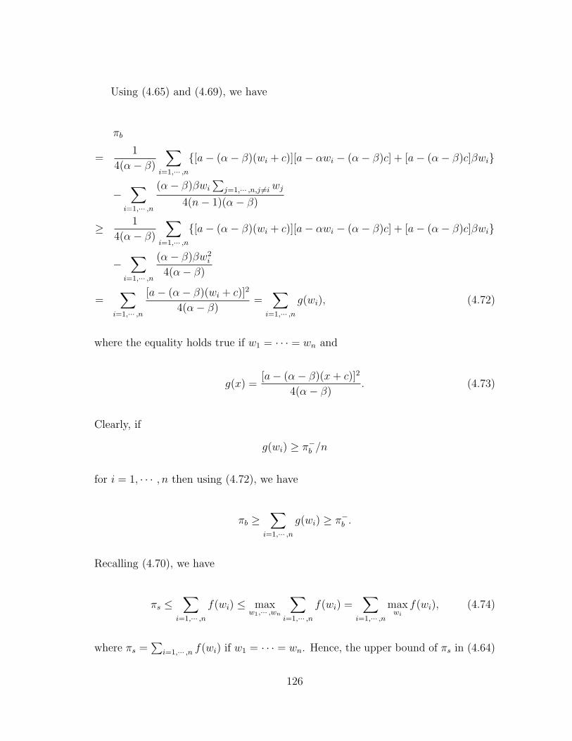
Using (4.65) and (4.69), we have
πb
=1
4(α− β)
∑i=1,··· ,n
{[a− (α− β)(wi + c)][a− αwi − (α− β)c] + [a− (α− β)c]βwi}
−∑
i=1,··· ,n
(α− β)βwi
∑j=1,··· ,n,j =iwj
4(n− 1)(α− β)
≥ 1
4(α− β)
∑i=1,··· ,n
{[a− (α− β)(wi + c)][a− αwi − (α− β)c] + [a− (α− β)c]βwi}
−∑
i=1,··· ,n
(α− β)βw2i
4(α− β)
=∑
i=1,··· ,n
[a− (α− β)(wi + c)]2
4(α− β)=
∑i=1,··· ,n
g(wi), (4.72)
where the equality holds true if w1 = · · · = wn and
g(x) =[a− (α− β)(x+ c)]2
4(α− β). (4.73)
Clearly, if
g(wi) ≥ π−b /n
for i = 1, · · · , n then using (4.72), we have
πb ≥∑
i=1,··· ,n
g(wi) ≥ π−b .
Recalling (4.70), we have
πs ≤∑
i=1,··· ,n
f(wi) ≤ maxw1,··· ,wn
∑i=1,··· ,n
f(wi) =∑
i=1,··· ,n
maxwi
f(wi), (4.74)
where πs =∑
i=1,··· ,n f(wi) if w1 = · · · = wn. Hence, the upper bound of πs in (4.64)
126

when πb ≥ π−b is satisfied is given by
∑i=1,··· ,n
maxwi
f(wi)
s.t. g(wi) ≥π−b
n, i = 1, · · · , n.
Let w∗i denote the optimal solution to the above optimization problem, i = 1, · · · , n.
Since this problem is separable based on wi, we have w∗i = w∗, i = 1, · · · , n, where
w∗ is the optimal solution to the following optimization problem
maxw
f(w) =(w − s)[a− (α− β)(w + c)]
2(4.75)
s.t. g(w) =[a− (α− β)(w + c)]2
4(α− β)≥ π−
b
n, (4.76)
using (4.71) and (4.73). It is important to note that this optimization problem is
the same as (Ps1) in the single-product setting, when b = α− β and the buyer’s
reservation profit is π−b /n.
Since wi = w∗, i = 1, · · · , n, using (4.74), πs = nf(w∗) =∑
i=1,··· ,nmaxwif(wi) =
nmaxw f(w). In this case, πs achieves its upper bound. Hence, the optimal whole-
sale price for product i under s1 in the symmetric n-product setting is given
by
ws1−nsi = w∗, (4.77)
i = 1, · · · , n, where w∗ is the optimal solution to (Ps1) in the single-product setting
with b = α− β and the buyer’s reservation profit is π−b /n.
4.3.2 Generic contract b3
Since the symmetric n-product setting is a generalization of the symmetric two-
product setting, the procedure of derivation for the optimal b3 should be the same.
127
One of the main differences in the derivation is to extend the ranges of indices
i, j = 1, 2 and j = i to i, j = 1, · · · , n and j = i. To avoid repetition, we summarize
the main results without presenting the details.
The expression of πs:
For given ki > 0 and mi ∈ ℜ, i = 1, · · · , n, using (4.40), the supplier’s profit πs
can be written as
πs =∑
i=1,··· ,n
(wi − s)
[a− α(kiwi +mi) +
β
n− 1
∑j=1,··· ,n,j =i
(kjwj +mj)
]. (4.78)
The buyer’s optimization problem:
The buyer’s optimization problem under b3 for the symmetric n-product
setting can be stated as
(Pb3− ns) : maxki>0,mi∈ℜ
πb =∑
i=1,··· ,n
[pb3−nsi (·)− wb3−ns
i (·)− c]qb3−nsi (·) (4.79)
s.t. pb3−nsi (·)− wb3−ns
i (·)− c ≥ 0,
siki +mi ≤a
α− β,
πs =∑
i=1,··· ,n
[wb3−ns
i (·)− s]qb3−nsi (·) ≥ π−
s , (4.80)
where wb3−nsi (·), pb3−ns
i (·), and qb3−nsi (·) are the supplier’s optimal response, i.e.,
the optimal wholesale price and the corresponding retail price and order
quantity for product i, i = 1, · · · , n and they are parameterized on ki and mi,
i = 1, · · · , n. In particular, wb3−nsi (·) can be computed by setting ∂πs/∂wi = 0 for
i = 1, · · · , n using (4.78), and pb3−nsi (·) and qb3−ns
i (·) can be then computed using
(4.40) and (4.56).
128

The optimal b3:
Inspired by the symmetric two-product setting and using the same approach, we
can show that the optimal contract parameters under b3 in the symmetric
n-product setting is such that
kb3−nsi =
Πc−n
π−s
and (4.81)
mb3−nsi = s+ c− sΠc−n
π−s
(4.82)
for i = 1, · · · , n. Note that Πc−n is the centralized optimal system profit defined in
(4.67).
Then, substituting (4.81) and (4.82) in (4.79) and (4.80), we have
πb3−nss = π−
s ,
πb3−nsb = Πc−n − π−
s , and
Πb3−ns = Πc−n.
Note that in the symmetric n-product setting, the optimal contracts parameters
are also free of the index i for i = 1, · · · , n. Once the centralized optimal system profit
Πc−n and the supplier’s reservation profit π−s are computed, the optimal contract
parameters can be decided using (4.81) and (4.82).
4.4 Relation between the multi-product and single-product contractual settings
In Section (4.3.1), we show that in the symmetric n-product setting, n ≥ 2, the
optimal wholesale prices for n products under s1 are the same as shown in (4.77).
The optimal wholesale price for each product can be solved using the optimization
problem given by (4.75) and (4.76). Recalling (Ps1) (the supplier’s problem under
129

s1) in the single-product setting, we find that the optimization problem given by
(4.75) and (4.76) is the same as (Ps1) when
• b = α − β, where b is the price sensitivity parameter in the demand function
q = a− bp in the single-product setting, and
• The buyer’s reservation profit in the single-product setting is given by π−b /n,
where π−b is the buyer’s reservation profit in the symmetric n-product setting.
Therefore, instead of solving a symmetric n-product problem, we can solve the corre-
sponding single-product problem and then the optimal decisions and resulting profits
for the former one can be easily obtained.
This fact is due to the symmetry of decisions for different products in the sym-
metric n-product setting. Letting wi = w, pi = p and qi = q, i = 1, · · · , n, the
demand function in (4.56) and the supplier’s and buyer’s profits in (4.57) and (4.58)
in the symmetric n-product setting can be reduced to
q = a− (α− β)p,
πs = n(w − s)[a− (α− β)p], and
πb = n(p− w − c)[a− (α− β)p].
From the above equations, we can see that the demand function in (4.56) becomes
the the single-product demand function, and both entities’ profits are n times their
profit on one product. Hence, the symmetric n-product problem becomes the single-
product problem.
Note that the demand function and the entities’ profits are only dependent on the
product substitution given by α − β and they are independent of individual values
of α and β. Recall that α represents the price sensitivity of demand, β represents
130

the price sensitivity of demand to a substitutable product in (4.56). Therefore, in
the symmetric n-product setting, we should focus on the difference of products’ price
sensitivities rather than the price sensitivity for each product individually.
In sum, using the results in the single-product setting under s1, we can solve a
symmetric n-product problem with the demand function in (4.56) and the buyer’s
reservation profit π−b in the following way:
• Consider a single-product setting with the demand function q = a− bp and the
buyer’s reservation profit π−0b . Set b = α− β and set π−0
b = π−b /n, n ≥ 2.
• Derive the optimal wholesale price under s1 in the single-product setting and
calculating the resulting profits for the supplier and the buyer.
• Then, in the symmetric n-product setting, the optimal wholesale price for each
product is the same as that in the single-product setting, while the supplier
(buyer)’s profit is n times that in the single-product setting, n ≥ 2.
In Section (4.3.2), we also show that the optimal decisions under b3 are same
for n products in the symmetric n-product setting. Hence, the symmetric n-product
problem under b3 can be also reduced to the single-product problem, and, hence,
the existing results in the single-product setting can be utilized in the symmetric
n-product setting under b3.
4.5 Modeling the case of asymmetric two products
We next examine b3 in the asymmetric two-product setting. The procedure of
derivation for the optimal b3 is the same as that in the symmetric two-product setting
discussed previously. To avoid repetition, we summarize the main steps and the main
results in asymmetric two-product setting.
131

Profit functions:
In the asymmetric two-product setting, the supplier’s profit function is given by
πs =∑i=1,2
(wi − si)qi =∑
i,j=1,2,i =j
(wi − si)(ai − αipi + βipj). (4.83)
The buyer’s profit function is given by
πb =∑i=1,2
(pi − wi − ci)qi =∑
i,j=1,2,j =i
(pi − wi − ci)(ai − αipi + βipj). (4.84)
We assume αi and βi are such that
αi > βi ≥ 0 and 4α1α2 − (β1 + β2)2 > 0, (4.85)
i = 1, 2. The first inequality in (4.85) is assumed based on the nature of price
competition, i.e., a product’s demand impacted by its own price more heavily than
by its competitor’s price. The second inequality ensures a property of πs as we
demonstrate next.
The expression of πs:
For given ki > 0 and mi ∈ ℜ, i = 1, 2, using (4.40), πs in (4.83) can be rewritten
as
πs =∑
i,j=1,2,i=j
(wi − si)[ai − αikiwi + βikjwj − (αimi − βimj)]. (4.86)
132

Compute the supplier’s optimal response:
Note that the Hessian matrix of πs in (4.86) is given by
∂2πs
∂w21
∂2πs
∂w1∂w2
∂2πs
∂w2∂w1
∂2πs
∂w22
=
−2α1k1 β1k2 + β2k1
β2k1 + β1k2 −2α2k2
.
The determinant of the Hessian matrix is given by
4α1α2k1k2 − (β1k2 + β2k1)2.
Here, we momentarily assume this quantity is greater than zero, and, hence, the
Hessian matrix is negative-definite. Later, we will show that under the optimal
contract the buyer would set k1 = k2, so that the determinant above reduces to
[4α1α2 − (β1 + β2)
2]k21 > 0,
since k1 > 0 by definition and (4.85).
Setting ∂πs/∂wi = 0 for i = 1, 2, we obtain the supplier’s optimal optimal
response, i.e., the optimal wholesale price for product i under b3, denoted
by
wb3−2ai (·). (4.87)
Using (4.40) and (4.1), the corresponding retail price and order quantity for
product i are given by
pb3−2ai (·) = kiw
b3−2ai (·) +mi and (4.88)
qb3−2ai (·) = ai − αip
b3−2ai (·) + βip
b3−2aj (·), (4.89)
133

i, j = 1, 2 and j = i.
The buyer’s optimization problem:
Note that using (4.1), pi can be written as a function of order quantities such
that
pi =aiαj + ajβi
α1α2 − β1β2
− αjqiα1α2 − β1β2
− βiqjα1α2 − β1β2
, (4.90)
i, j = 1, 2 and j = i.
Using (4.83), (4.84), and (4.90), in order to guarantee qi ≥ 0 and the sup-
plier’s and buyer’s profits on product i are nonnegative, we assume pi ≤ (aiαj +
ajβi)/(α1α2 − β1β2), wi ≥ si, and pi ≥ wi + ci so that
siki +mi ≤ kiwi +mi = pi ≤aiαj + ajβi
α1α2 − β1β2
and pb3−2ai (·)− wb3−2a
i (·)− ci ≥ 0,(4.91)
i = 1, 2. We refer to (4.91) as the main constraint on the decision variables of the
contract design problem under b3 in the asymmetric two-product setting.
Then, the buyer’s optimization problem under b3 for the asymmetric
two-product setting can be stated as
(Pb3− 2a) : maxki>0,mi∈ℜ
πb =∑i=1,2
[pb3−2ai (·)− wb3−2a
i (·)− ci]qb3−2ai (·) (4.92)
s.t. pb3−2ai (·)− wb3−2a
i (·)− ci ≥ 0
siki +mi ≤aiαj + ajβi
α1α2 − β1β2
πs =∑i=1,2
[wb3−2a
i (·)− si]qb3−2ai (·) ≥ π−
s , (4.93)
where wb3−2ai (·), pb3−2a
i (·), and qb3−2ai (·) are given by (4.87), (4.88), and (4.89), i =
134

1, 2.
The optimal b3:
We apply the same approach as that in the symmetric two-product setting to
identify the optimal contract parameters in the asymmetric two-product setting.
Inspired by the optimal contract in the symmetric two-product setting, we consider
the tuple (kb3−2ai ,mb3−2a
i ) such that
kb3−2ai =
Πc−2a
π−s
and (4.94)
mb3−2ai = si + ci −
siΠc−2a
π−s
, (4.95)
i = 1, 2. Note that Πc−2a is the centralized optimal system profit, which can be
calculated by
Πc−2a = maxpi∈
[si+ci,
aiαj+ajβiα1α2−β1β2
],i=1,2
Π =∑
i,j=1,2,j =i
(pi − si − ci)(ai − αipi + βipj).
Then, substituting (4.94) and (4.95) in (4.92) and (4.93), we have
πb3−2as = π−
s ,
πb3−2ab = Πc−2a − π−
s , and (4.96)
Πb3−2a = πb3−2as + πb3−2a
b = Πc−2a.
We have πb3−2ab ≥ 0 in (4.96) for π−
s ∈ [0,Πc−2a]. Hence, the tuple given by (4.94)
and (4.95) is a feasible solution under which the buyer obtains the upper bound of
the objective function in (4.92). Therefore, the tuple is also optimal.
It is important to note that in the asymmetric two-product setting, we have
135

kb3−2a1 = kb3−2a
2 while mb3−2a1 = mb3−2a
2 is possible using (4.94) and (4.95). Although
one may expect that the asymmetric two-product problem is difficult to solve, as
we can see, the optimal contract parameters under b3 are easy to calculate. Since
the transaction between the supplier and the buyer is only based on the wholesale
payment, the contract is also easy to implement.
4.6 Conclusion
In this chapter, we generalize the basic single-product setting to consider multiple
symmetric and asymmetric substitutable products. Since there is no previous work
on the buyer-driven channel in this setting, we focus on examine the buyer-driven
generic contract b3 in the two-product symmetric case, n-product symmetric case,
and two-product asymmetric case. Our results document the conditions under which
the generic contract remains to be a simple, yet, effective contract when multiple
substitutable products are considered.
136

5. THE GENERIC CONTRACT IN THE EXCLUSIVE DEALER SETTING
5.1 Setting 3. The exclusive dealer contractual setting
This chapter revisits the two-product channel with two suppliers and two buy-
ers, where each supplier (e.g., manufacturer) produces one product and each buyer
(e.g., dealer) sells one supplier’s product exclusively. This channel, referred as the
exclusive dealer setting (Choi (1996)) here, is illustrated in Figure 5.1. Supplier
i’s decision pertains to the wholesale price wi, and buyer i’s decisions pertain to the
order quantity qi and retail price pi for product i, i = 1, 2. We assume a generalized
linear demand function for product i given by
qi = ai − αipi + βipj, (5.1)
i, j = 1, 2, and i = j. As in Chapter 4, ai presents the maximum demand of product
i when prices for both products approach zero (McGuire and Staelin (1983)), and αi
and βi represent the sensitivity of demand for product i to its retail price and to the
substitutable product’s retail price (Ingene and Parry (2004)), respectively, i = 1, 2.
Let si and ci denote supplier i’s unit production cost and buyer i’s unit distribution
cost, respectively, i = 1, 2. The notation introduced so far and used frequently in
the remainder of this chapter is summarized in Table 5.1. Note that we consider the
generalized asymmetric case. It is the case where all parameters in (5.1) and costs of
different products are different, i.e., a1 = a2, α1 = α2, β1 = β2, s1 = s2, and c1 = c2.
5.2 Supplier- and buyer-driven contracts
In Chapter 3, we have studied three buyer-driven contracts and a supplier-driven
contract in the basic single-product setting. Now, we are interested in the same
137

Buyer 1Supplier 1 w1
w2
p1, q1 = a1 � α1p1 + �1p2
p2, q2 = a2 – α2p2 + β2p1
Supplier 2 Buyer 2
Figure 5.1: The exclusive dealer contractual setting.
Table 5.1: Summary of notation in the exclusive dealer setting.
Symbol Explanationi the index of a product, i = 1, 2pi the retail price for product iqi the demand for product i, qi = ai − αipi + βipj, j = 1, 2, j = iαi the sensitivity of qi to piβi the sensitivity of qi to pj, j = 1, 2, j = iwi the wholesale price for product isi supplier i’s unit production costci buyer i’s unit distribution costki the price multiplier for product i, ki > 0mi the price margin for product i, mi ∈ ℜ
contracts in the exclusive dealer setting as follows:
b1. Under the margin-only contract, buyer i decides the price margin of product
i, denoted by mi, mi ≥ 0, representing the difference between the retail and
wholesale prices of product i, i = 1, 2. Also, buyer i commits that the retail
price of product i would be set such that pi = wi +mi and its order quantity
would be set such that qi = a − αpi + βpj = a − α(wi + mi) + β(wj + mj),
i, j = 1, 2 and j = i. Next, supplier i decides wi, i = 1, 2.
b2. Under the multiplier-only contract, buyer i decides the price multiplier of prod-
uct i, denoted by ki, ki ≥ 1, representing the ratio of the retail and wholesale
138

prices of product i, i = 1, 2. Also, buyer i commits that the retail price of
product i would be set such that pi = kiwi and its order quantity would be set
such that qi = a− αpi + βpj = a− αkiwi + βkjwj, i, j = 1, 2 and j = i. Next,
supplier i decides wi, i = 1, 2.
b3. Under the generic contract, buyer i decides on the valuesa of ki and mi, ki > 0
and mi ∈ ℜ, while also committing that the retail price of product i would
be set such that pi = kiwi +mi and its order quantity would be set such that
qi = a − αpi + βpj = a − α(kiwi +mi) + β(kjwj +mj), i, j = 1, 2 and j = i.
Next, supplier i decides wi, i = 1, 2.
s1. Under the wholesale price contract with Cournot competition, supplier i decides
wi and then buyer i decides qi, i = 1, 2.
We are interested in computing the optimal contract parameters under these
contracts. To this end, we develop optimization models and examine the contracts
in the buyer-driven channel using the following approach:
• (Vertical Stackelberg game) the buyer tier takes the lead and offers a contract
first and then the supplier tier follows. See the definition of Stackelberg game
in Chapter 1.
• (Horizontal Nash game) the two entities in a tier have the same negotiation
power and make decisions simultaneously. See the discussion of Horizontal
Nash game given by Ingene and Parry (2004).
aObserve that, under b3, mi can be positive or negative representing a margin (mark-up) orrebate (mark-down). Likewise, under b3, ki is allowed to be positive or negative for the sake ofgenerality. However, in the basic single-product setting in Chapter 3, we already show that theoptimal multiplier is positive due to the natural and practical assumptions of the contractual settingat hand. Hence, we only consider ki > 0 in the exclusive dealer setting.
139

The exclusive dealer setting of interest has appeared in the literature (e.g., McGuire
and Staelin (1983), Lee and Staelin (1997), Trivedi (1998), Zhang et al. (2012), Li
et al. (2013), and Feng and Lu (2013)). Of particular interest for us are the results
presented by Lee and Staelin (1997), Trivedi (1998), and Zhang et al. (2012) who
examine the same approach as ours in the buyer-driven channel.
Lee and Staelin (1997) consider a buyer-driven contract under which the buyers
decide the price margins (the difference of pi and wi), i.e., pi − wi, simultaneously,
first, and then the suppliers decide the manufacture margins (the difference of wi and
si), i.e., wi−si, simultaneously, i = 1, 2. Lee and Staelin (1997) assume a symmetric
demand function between the two products satisfying that “demand for a product
is decreasing in its own retail price and increasing in or independent of other retail
prices” (Lee and Staelin (1997)). They also assume symmetric costs for the suppliers
and ignore the buyers’ costs, i.e., s1 = s2 and c1 = c2 = 0.
Lee and Staelin (1997) compare the buyer-driven contract with a supplier-driven
contract under which the suppliers decide the manufacture margins first and then the
buyers decide the price margins. They demonstrate that each entity is better off to
possess leadership. They also show that suppliers’ and buyers’ profits are symmetric
under different leaderships, i.e., the leaders (followers)’ profits are the same under
both leaderships. In addition, the retail prices and the system profits under different
leaderships are the same, i.e., the system efficiency is independent of whether the
suppliers or the buyers play as channel leaders.
Trivedi (1998) considers a buyer-driven contract under which the buyers decide
the price margins, i.e., pi − wi, simultaneously, first, and then the suppliers decide
wi simultaneously, i = 1, 2. The demand function in the paper is a special case
of (5.1) where a1 = a2 = 1 and α1 = α2 = 1, and all costs are ignored, i.e.,
s1 = s2 = c1 = c2 = 0. Trivedi (1998) compares the buyer-driven contract with
140

a supplier-driven contract under which the suppliers decide wholesale prices first
and then the buyers decide the price margins. Trivedi (1998) also conclude that
leadership is always beneficial.
Zhang et al. (2012) generalize Trivedi (1998) by using a linear demand function
with one asymmetric parameter. The demand function is still a special case of (5.1)
where ai = (Ai − θAj)/(1− θ2), α1 = α2 = 1/(1− θ2), and β1 = β2 = θ/(1− θ2), Ai,
Aj, and θ are constants defined in Zhang et al. (2012), i, j = 1, 2 and j = i. They
derive the optimal solutions for the supplier- and buyer-driven contracts assuming
the asymmetric parameter Ai, i = 1, 2, and compare the two contracts under the
symmetric case when A1 = A2. Similar to Trivedi (1998), Zhang et al. (2012)
also show that leadership is always beneficial. They also demonstrate that which
leadership results in more system profit depends on the product substitutability.
Note that all the three papers that use the same approach as ours consider a
buyer-driven contract under which the buyers announce the price margins first and
then the suppliers decide wi, or equivalently, wi−si, i = 1, 2. This contract is referred
to as the margin-only contract here. However, the current literature does not concern
whether deciding on margins is optimal for the buyers and generally overlooks other
buyer-driven contracts. Also, they either consider the fully symmetric case or have
symmetric assumptions. Moreover, they do not take into account reservation profits
for entities. To extend the current literature, in this chapter, we study a more general
buyer-driven contract (i.e., the generic contract) in the generalized asymmetric case
based on the following consideration:
• A general contract with more contract flexibility may improve the profit po-
tential for the buyers, and
• The consideration of the generalized asymmetric case provides an extension of
141
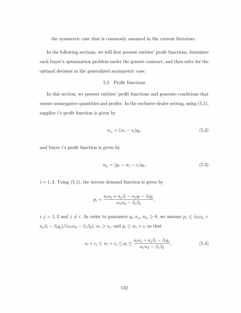
the symmetric case that is commonly assumed in the current literature.
In the following sections, we will first present entities’ profit functions, formulate
each buyer’s optimization problem under the generic contract, and then solve for the
optimal decision in the generalized asymmetric case.
5.3 Profit functions
In this section, we present entities’ profit functions and generate conditions that
ensure nonnegative quantities and profits. In the exclusive dealer setting, using (5.1),
supplier i’s profit function is given by
πsi = (wi − si)qi, (5.2)
and buyer i’s profit function is given by
πbi = (pi − wi − ci)qi, (5.3)
i = 1, 2. Using (5.1), the inverse demand function is given by
pi =aiαj + ajβi − αjqi − βiqj
α1α2 − β1β2
,
i, j = 1, 2 and j = i. In order to guarantee qi, πsi , πbi ≥ 0, we assume pi ≤ (aiαj +
ajβi − βiqj)/(α1α2 − β1β2), wi ≥ si, and pi ≥ wi + ci so that
si + ci ≤ wi + ci ≤ pi ≤aiαj + ajβi − βiqj
α1α2 − β1β2
, (5.4)
142

i, j = 1, 2 and j = i. We assume when retail prices for both products are set at their
lower bounds, i.e., p1 = s1 + c1 and p2 = s2 + c2, we have q1, q2 ≥ 0 so that
ai − αi(si + ci) + βi(sj + cj) ≥ 0 (5.5)
using (5.1), i, j = 1, 2 and j = i. Following Chapter 4, we assume αi > βi ≥ 0,
i = 1, 2.
5.4 The generic contract in the generalized asymmetric case
Recall that under b3, buyer i announces that pi would be set depending on wi
according to
pi = kiwi +mi, (5.6)
where ki > 0 and mi ∈ ℜ is the unconstrained value representing a margin (mark-
up) or rebate (mark-down), i = 1, 2. Then, the buyers move first and decide ki and
mi, and the suppliers select optimal wi, i = 1, 2. Next, we proceed with a formal
formulation of each buyer’s optimization problem given the other buyer’s decision
under b3.
5.4.1 Formulation of (Pb3− ai)
In the sequential leader-follower game, the buyers make decisions by predict-
ing the suppliers’ best responses. In order to formulate each buyer’s optimization
problem, we need to examine the suppliers’ best responses on w1 and w2 for given
k1, k2 > 0 and m1,m2 ∈ ℜ.
For given k1, k2 > 0 and m1,m2 ∈ ℜ, supplier i decides the optimal wi corre-
sponding to wj and then pi and qi are determined by wi, i, j = 1, 2 and j = i. We
first need to identify the conditions on wi, pi, and qi that ensure nonnegative profit
for supplier i for given wj, k1, k2 > 0 and m1,m2 ∈ ℜ, i, j = 1, 2 and j = i. After
143

obtaining the suppliers’ best responses and the corresponding pi and qi, we need to
verify the conditions are satisfied and then identify the constraint on k1, k2, m1, and
m2 for the verification.
Then, considering the suppliers’ best responses, buyer i decides the optimal ki
and mi, for given kj > 0 and mj ∈ ℜ, i, j = 1, 2 and j = i. To formulate buyer i’s
problem, we also need to identify the constraint on ki and mi for given kj > 0 and
mj ∈ ℜ that ensure nonnegative profit for buyer i, i, j = 1, 2 and j = i.
Following this logic, now, we start with identifying the conditions on wi, pi, and
qi for given wj, k1, k2 > 0 and m1,m2 ∈ ℜ, i, j = 1, 2 and j = i. Substituting (5.6)
in (5.1), we have
qi = ai − αi(kiwi +mi) + βi(kjwj +mj) ≥ 0,
and, hence,
kiwi +mi ≤ai + βi(kjwj +mj)
αi
, (5.7)
i, j = 1, 2 and j = i.
Since ki > 0, by assumption (5.4), (5.7) implies
siki +mi ≤ wiki +mi ≤ai + βi(kjwj +mj)
αi
, (5.8)
i, j = 1, 2 and j = i. Using (5.8) along with (5.7), we then conclude that ki, mi, wi,
144

and pi should be such that
siki +mi ≤ai + βi(kjwj +mj)
αi
, (5.9)
si ≤ wi ≤ai + βi(kjwj +mj)
αiki− mi
ki, and (5.10)
siki +mi ≤ pi ≤ai + βi(kjwj +mj)
αi
, (5.11)
i, j = 1, 2 and j = i. Note that if (5.11) is true then (5.9) is true. Also, recalling
(5.1) and assumption (5.4), we have
0 ≤ qi ≤ ai − αi(si + ci) + βi(kjwj +mj), (5.12)
i, j = 1, 2 and j = i.
Next, we derive the suppliers’ best responses. Let us examine πsi in (5.2) under
b3, i = 1, 2. For given values of k1, k2 > 0 and m1,m2 ∈ ℜ, using (5.1) and (5.6), πsi
in (5.2) can be rewritten as
πsi = (wi − si)qi = (wi − si)[ai − αikiwi + βikjwj − (αimi − βimj)], (5.13)
so that
dπsi
dwi
= ai − 2αikiwi + βikjwj − (αimi − βimj) + kiαisi and (5.14)
d2πsi
dw2i
= −2αiki < 0,
i, j = 1, 2 and j = i. Hence, πsi in (5.13) is concave in wi, i = 1, 2. Setting
145

dπs1/dw1 = dπs2/dw2 = 0 in (5.14) leads to
wb3i (·) =
2aiαj + ajβi + 2α1α2(siki −mi) + β1β2mi + αjβi(sjkj +mj)
(4α1α2 − β1β2)ki, (5.15)
where wb3i (·) which is parameterized on k1, k2, m1, and m2 is a simplified notation
for wb3i (k1, k2,m1,m2), i, j = 1, 2 and j = i.
Now, we verify whether wb3i (·) is realizable over the region (5.10). Observe that
for given k1, k2 > 0, m1,m2 ∈ ℜ, we have
ai + βi(kjwb3j (·) +mj)
αiki− mi
ki− wb3
i (·) = wb3i (·)− si =
Wi
(4α1α2 − β1β2)ki,
where
Wi = 2aiαj + ajβi − (2α1α2 − β1β2)(siki +mi) + αjβi(sjkj +mj), (5.16)
i, j = 1, 2 and j = i. Hence, if
Wi ≥ 0 (5.17)
then wb3i (·) defined in (5.15) is supplier i’s optimal response, i.e., the optimal
wholesale price, under b3, for given values of k1, k2 > 0 and m1,m2 ∈ ℜ, because
it is realizable over the region (5.10), i, j = 1, 2 and j = i. Substituting (5.15) in
(5.6) and using (5.1), the corresponding retail price and order quantity for
146

product i for given values of k1, k2 > 0 and m1,m2 ∈ ℜ are given by
pb3i (·) = kiwb3i (·) +mi
=2aiαj + ajβi + αjβi(sjkj +mj) + 2α1α2(siki +mi)
4α1α2 − β1β2
and (5.18)
qb3i (·) = ai − αi[kiwb3i (·) +mi] + βi[kjw
b3j (·) +mj]
=αiWi
4α1α2 − β1β2
, (5.19)
respectively, where pb3i (·) and qb3i (·) are also parameterized on k1, k2, m1, and m2,
and Wi is given by (5.16), i, j = 1, 2 and j = i. Again, since we assume (5.17),
ai + βi(kjwb3j (·) +mj)
αi
− pb3i (·) =Wi
4α1α2 − β1β2
≥ 0 and
pb3i (·)− siki −mi =Wi
4α1α2 − β1β2
≥ 0,
so that pb3i (·) defined in (5.18) lies over the region (5.11), where Wi is defined in
(5.16), i, j = 1, 2 and j = i. Likewise,
ai − αi(si + ci) + βi(kjwb3j (·) +mj)− qb3i (·) =
αiWi
4α1α2 − β1β2
≥ 0,
so that qb3i (·) defined in (5.19) lies over the region (5.12), i, j = 1, 2 and j = i.
Last but not least, we need to verify that assumption (5.4) holds true for wb3i (·),
where wb3i (·) is as defined in (5.15), i = 1, 2. Similar to the generic contract in the
single-product setting, the constraint (5.17) derived earlier is not sufficient to verify
this under b3. For this reason, recalling assumption (5.4) and using (5.6) and (5.15),
we need to ensure
si + ci ≤ wb3i (·) + ci ≤ kiw
b3i (·) +mi ≤
aiαj + ajβi − βiqjα1α2 − β1β2
(5.20)
147

holds true. Examining the above inequalities, if (5.17) is true and
(ki − 1)wb3i (·) +mi − ci ≥ 0
then (5.20) is ensured, i = 1, 2. Obviously, the inequality above is equivalent to
(ki − 1)[2aiαj + ajβi + 2α1α2(siki −mi) + β1β2mi + αjβi(sjkj +mj)]
(4α1α2 − β1β2)ki+mi− ci ≥ 0,
(5.21)
i, j = 1, 2 and j = i. Hence, we refer to (5.17) and (5.21) as the main constraints
of the problem at hand.
Using (5.15), (5.18), and (5.19) in (5.2) and (5.3), we have
πsi =αi[2aiαj + ajβi − (2α1α2 − β1β2)(siki +mi) + αjβi(sjkj +mj)]
2
(4α1α2 − β1β2)kiand
πbi =αi[2aiαj + ajβi − (2α1α2 − β1β2)(siki +mi) + αjβi(sjkj +mj)]
4α1α2 − β1β2
·
{(ki − 1)[2aiαj + ajβi + 2α1α2(siki −mi) + β1β2mi + αjβi(sjkj +mj)]
(4α1α2 − β1β2)ki
+mi − ci
},
i, j = 1, 2 and j = i.
Although ki > 0 by definition, in order to apply Karush-Kuhn-Tucker (KKT)
conditions (Bazaraa et al. (2006)), under which a strict inequality constraint is not
allowed, to solve buyer i’s optimization problem as shown below, we momentarily
assume ki ∈ ℜ, i = 1, 2. We solve the optimal decision over ki,mi ∈ ℜ and then
show that the optimal ki is actually positive, i = 1, 2.
Considering the fact that b3 is a buyer-driven contract, supplier i would not
accept b3 unless supplier i’s corresponding profit exceeds the reservation profit π−si,
148

i = 1, 2. Recalling (5.17) and (5.21) and considering the above expressions for πsi
and πbi and ki,mi ∈ ℜ, buyer i’s optimization problem under b3 can be stated
as
(Pb3− ai) :
maxki,mi∈ℜ
πbi
=αi[2aiαj + ajβi − (2α1α2 − β1β2)(siki +mi) + αjβi(sjkj +mj)]
4α1α2 − β1β2
·
{(ki − 1)[2aiαj + ajβi + 2α1α2(siki −mi) + β1β2mi + αjβi(sjkj +mj)]
(4α1α2 − β1β2)ki
+mi − ci
}(5.22)
s.t., 2aiαj + ajβi − (2α1α2 − β1β2)(siki +mi) + αjβi(sjkj +mj) ≥ 0,
(ki − 1)[2aiαj + ajβi + 2α1α2(siki −mi) + β1β2mi + αjβi(sjkj +mj)]
(4α1α2 − β1β2)ki
+mi − ci ≥ 0,
πsi =αi[2aiαj + ajβi − (2α1α2 − β1β2)(siki +mi) + αjβi(sjkj +mj)]
2
(4α1α2 − β1β2)ki
≥ π−si, (5.23)
given kj,mj ∈ ℜ, i, j = 1, 2 and j = i.
As discussed earlier, under b3 buyer 1 and buyer 2 make decisions simultaneously,
and, hence, their optimal decisions lead to a Nash equilibrium (Fudenberg and Tirole
(1991)). That is, each buyer does not have an incentive to deviate if the other buyer’s
decision is fixed. In the following, we will characterize the Nash equilibrium in three
steps:
• First, for given kj,mj ∈ ℜ, we use KKT necessary conditions to identify a KKT
point (see the definition of KKT point in Bazaraa et al. (2006)) for (Pb3− ai),
i, j = 1, 2 and j = i. The reason for doing this is the following: According to
149

Lemma 4.4.1 of Bazaraa et al. (2006), if the Hessian of the Lagrangian function
conditioned on Lagrangian multipliers associated with a KKT point is negative
semi-definite in the feasible region, then the KKT point is a global maximum.
• Second, using Lemma 4.4.1 of Bazaraa et al. (2006), we show that the KKT
point is optimal for (Pb3− ai) given kj,mj ∈ ℜ, i, j = 1, 2 and j = i.
• Finally, using the optimal response of each buyer corresponding to the other
buyer’s decision, we identify the Nash equilibrium of the two buyers’ optimiza-
tion problems.
5.4.2 Optimal solution of (Pb3− ai)
We start with identifying a KKT point for (Pb3−ai), i = 1, 2. Let µi1, µi2, and µi3
denote Lagrangian multipliers corresponding to the three constraints in (Pb3− ai),
respectively, i = 1, 2. The Lagrangian function is given by
Li = Li(ki,mi, µi1, µi2, µi3) = πbi + µi1gi1 + µi2gi2 + µi3gi3, (5.24)
where
gi1 = 2aiαj + ajβi − (2α1α2 − β1β2)(siki +mi) + αjβi(sjkj +mj), (5.25)
gi2 =(ki − 1)[2aiαj + ajβi + 2α1α2(siki −mi) + β1β2mi + αjβi(sjkj +mj)]
(4α1α2 − β1β2)ki
+mi − ci, and (5.26)
gi3 = πsi − π−si, (5.27)
and πbi and πsi are given by (5.22) and (5.23), respectively, i, j = 1, 2 and j = i.
Thus, the KKT necessary conditions (see Theorem 4.2.13 in Bazaraa et al. (2006))
150

are the following:
∂Li
∂ki=
∂πbi
∂ki+ µi1
∂gi1∂ki
+ µi2∂gi2∂ki
+ µi3∂gi3∂ki
= 0, (5.28)
∂Li
∂mi
=∂πbi
∂mi
+ µi1∂gi1∂mi
+ µi2∂gi2∂mi
+ µi3∂gi3∂mi
= 0, (5.29)
∂Li
∂µi1
= gi1 ≥ 0, (5.30)
∂Li
∂µi2
= gi2 ≥ 0, (5.31)
∂Li
∂µi3
= gi3 ≥ 0, (5.32)
µi1gi1 = 0, (5.33)
µi2gi2 = 0, (5.34)
µi3gi3 = 0, (5.35)
µi1, µi2, µi3 ≥ 0, i = 1, 2. (5.36)
Then, we characterize the Lagrangian multipliers that satisfy (5.28) – (5.36) at
optimality, denoted by µ∗i1, µ
∗i2, and µ∗
i3, i = 1, 2. We first show µ∗i1 = µ∗
i2 = 0 is true,
i = 1, 2. Consider all possible cases of µ∗i1 and µ∗
i2, i = 1, 2:
1. If µ∗i1 > 0 and µ∗
i2 = 0 then by (5.33) gi1 = 0. Using (5.25) in (5.22) and (5.23),
gi1 = 0 implies πbi = πsi = 0. If π−si
> 0 then there does not exist a feasible
solution. If π−si= 0 then obviously the solution for the KKT conditions is not
optimal.
2. If µ∗i1 = 0 and µ∗
i2 > 0 then by (5.34) gi2 = 0. Using (5.26) in (5.22), gi2 = 0
implies πbi = 0. Obviously, the solution for the KKT conditions is not optimal.
3. If µ∗i1 > 0 and µ∗
i2 > 0 then by (5.33) and (5.34) gi1 = gi2 = 0. According to
151

the development of (5.25) and (5.26),
gi1 = 0 ⇔ wb3i (·) = si and gi2 = 0 ⇔ (ki − 1)wb3
i (·) +mi − ci = 0.
Hence,
gi1 = gi2 = 0 ⇔ (ki − 1)si +mi − ci = 0 ⇔ kisi +mi = si + ci.
Using kisi +mi = si + ci in (5.25), gi1 = 0 is equivalent to
Ai = 2aiαj + ajβi − (2α1α2 − β1β2)(si + ci) + αjβi(sjkj +mj) = 0, (5.37)
j = 1, 2, j = i.
• If Ai = 0 then the solution should satisfy kisi +mi = si + ci. Note that
gi1 = gi2 = 0 implies πbi = πsi = 0. If π−si> 0 then there does not exist
a feasible solution. If π−si
= 0 then obviously the solution for the KKT
conditions is not optimal.
• Otherwise if Ai = 0 then there does not exist a solution for gi1 = gi2 = 0.
Therefore, the three cases above are ruled out, and at optimality we have µ∗i1 = µ∗
i2 =
0, i = 1, 2. Next, we analyze the solution of (5.28) – (5.36) assuming µ∗i1 = µ∗
i2 = 0
for two different cases:
Case 0: µ∗i1 = µ∗
i2 = 0 and µ∗i3 > 0;
Case 1: µ∗i1 = µ∗
i2 = 0 and µ∗i3 = 0, i = 1, 2.
152

Case 0.
If µ∗i1 = µ∗
i2 = 0 and µ∗i3 > 0 then (5.28) and (5.29) reduce to
∂Li
∂ki=
∂πbi
∂ki+ µ∗
i3
∂gi3∂ki
=∂πbi
∂ki+ µ∗
i3
∂πsi
∂ki= 0, (5.38)
∂Li
∂mi
=∂πbi
∂mi
+ µ∗i3
∂gi3∂mi
=∂πbi
∂mi
+ µ∗i3
∂πsi
∂mi
= 0, (5.39)
and using (5.27), (5.35) implies
πsi = π−si, (5.40)
i = 1, 2.
Then, we solve µ∗i3 such that (5.38) – (5.40) are satisfied at the point (ki,mi) =
(k∗i (kj,mj),m
∗i (kj,mj)). Using (5.22) and (5.23), we have
∂πbi
∂ki=
αi
(4α1α2 − β1β2)2k2i
{αjβ2i (sjkj +mj)[αj(sjkj +mj) + βjsik
2i ]
+(2aiαj + ajβi)[2aiαj + ajβi + 2βiαj(sjkj +mj)]
+sik2i (β
21β
22ci + 8α2
1α22ci − 6α1α2β1β2ci + 2aiαjβ1β2 + ajβ
2i βj)
−(2α1α2 − β1β2)[2αjβimi(sjkj +mj) + 4α1α2sik2i (siki +mi)
+2mi(2aiαj + ajβi)−m2i (2α1α2 − β1β2)− 2α1α2s
2i k
2i ]},
∂πbi
∂mi
= − αi
(4α1α2 − β1β2)2ki{[ki(ajβ2
i βj − 6α1α2β1β2ci + 8α21α
22ci + β2
1β22ci
+2aiαjβ1β2)] + αjβi(sjkj +mj)(4α1α2 − 2β1β2 + kiβ1β2)
+2(2α1α2 − β1β2)(2aiαj + ajβi)− 4kiα1α2(2α1α2 − β1β2)(kisi +mi)
+2α1α2(β1β2siki − 4α1α2mi + 2β1β2mi)}, (5.41)
∂πsi
∂ki= −αigi1[2aiαj + ajβi + (2α1α2 − β1β2)(kisi −mi) + αjβi(kjsj +mj)]
(4α1α2 − β1β2)2k2i
, and
∂πsi
∂mi
= −2αigi1(2α1α2 − β1β2)
(4α1α2 − β1β2)2ki,
153

i, j = 1, 2 and j = i. Substituting the above equations in (5.38) – (5.40) and solving
the problem using the software Maple 14, we obtain
µ∗i3 = 1,
k∗i (kj,mj) =
A2i
16αiα2jπ
−si
, and (5.42)
m∗i (kj,mj) =
β1β2[2aiαj + ajβi + αjβi(sjkj +mj)]
4α1α2(2α1α2 − β1β2)
+(2α1α2 − β1β2)(4α1α2 − β1β2)(si + ci)
4α1α2(2α1α2 − β1β2)
−sik∗i (kj,mj), (5.43)
where Ai is defined in (5.37), i, j = 1, 2 and j = i.
Next, in order to show that (k∗i (kj,mj),m
∗i (kj,mj)) is a KKT point, we need to
verify whether (5.30) and (5.31) are satisfied for ki = k∗i (kj,mj) andmi = m∗
i (kj,mj),
i, j = 1, 2 and j = i. Substituting (5.42) and (5.43) in (5.25) and (5.26), we have
gi1 =(4α1α2 − β1β2)Ai
4α1α2
and
gi2 =(4α1α2 − β1β2)[A
2i − 8αj(2α1α2 − β1β2)π
−si]Ai
32αiα2j (2α1α2 − β1β2)π−
si
,
where Ai is defined in (5.37), i, j = 1, 2 and j = i. As we can see, gi1, gi2 ≥ 0 is true
only if
Ai ≥ 0 and (5.44)
π−si∈[0,
A2i
8αj(2α1α2 − β1β2)
], (5.45)
i, j = 1, 2 and j = i.
Therefore, the KKT necessary conditions in (5.28)–(5.36) are all satisfied for
154

(ki,mi) = (k∗i (kj,mj),m
∗i (kj,mj)) and (µ∗
i1, µ∗i2, µ
∗i3) = (0, 0, 1), if (5.44) and (5.45)
hold true, i, j = 1, 2 and j = i. According to Bazaraa et al. (2006), the solution
(k∗i (kj,mj),m
∗i (kj,mj)) is a KKT point with Lagrangian multipliers (µ∗
i1, µ∗i2, µ
∗i2)
corresponding to the three constraints in (Pb3− ai), if (5.44) and (5.45) hold true,
i, j = 1, 2 and j = i.
Substituting (5.42) and (5.43) in (5.22), buyer i’s corresponding profit at the
KKT point is given by
π∗bi=
A2i
8αj(2α1α2 − β1β2)− π−
si, (5.46)
i = 1, 2. Since the constraint on supplier i’s profit is binding as seen in (5.40),
supplier i’s correponding profit is the reservation profit, i = 1, 2.
Case 1.
If µ∗i1 = µ∗
i2 = µ∗i3 = 0 then (5.28) and (5.29) reduce to ∂πbi/∂ki = 0 and
∂πbi/∂mi = 0, i = 1, 2. Setting ∂πbi/∂mi = 0 in (5.41), we obtain
mi(ki) =2(2α1α2 − β1β2)(2aiαj + ajβi)
2(2α1α2ki + 2α1α2 − β1β2)(2α1α2 − β1β2)
+αjβi(4α1α2 − 2β1β2 + kiβ1β2)(sjkj +mj)
2(2α1α2ki + 2α1α2 − β1β2)(2α1α2 − β1β2)
+(ajβ
2i βj + β2
1β22ci + 2aiαjβ1β2 + 8α2
1α22ci − 6α1α2β1β2ci)ki
2(2α1α2ki + 2α1α2 − β1β2)(2α1α2 − β1β2)
− (2α1α2 − β1β2)(4α1α2ki − β1β2)siki2(2α1α2ki + 2α1α2 − β1β2)(2α1α2 − β1β2)
,
i, j = 1, 2 and j = i. Substituting the above equation for mi in (5.22), we have
πbi =αikiA
2i
4(2α1α2ki + 2α1α2 − β1β2)(2α1α2 − β1β2), (5.47)
155
so that
∂πbi
∂ki=
αiA2i
4(2α1α2ki + 2α1α2 − β1β2)2≥ 0, (5.48)
where Ai is defined in (5.37), i, j = 1, 2 and j = i. Consider the following two cases
for Ai:
• If Ai = 0 then using (5.47) πbi = 0, i = 1, 2. Obviously, it is not optimal.
• Otherwise if Ai = 0 then using (5.48), ∂πbi/∂ki > 0 over −∞ < ki < +∞,
i = 1, 2. Hence, ∂πbi/∂ki = 0 is not true in general unless ki = ∞, i = 1, 2. In
this case, there is not finite solution for ∂πbi/∂ki = 0 such that−∞ < ki < +∞,
i = 1, 2. By (5.23), πsi ≥ 0 is true only if ki > 0, and, hence, we can omit
ki = −∞, i = 1, 2. Now, let us consider ki = +∞, i = 1, 2. Using (5.47), we
have
limki→+∞
πbi =A2
i
8αj(2α1α2 − β1β2),
where Ai is defined in (5.37), i = 1, 2. Substituting mi = mi(ki) in (5.23), we
have
πsi =αikiA
2i
4(2α1α2ki + 2α1α2 − β1β2)2,
so that
limki→+∞
πsi =αiA
2i
16(2α1α2ki + 2α1α2 − β1β2)α1α2
= 0,
i = 1, 2. Therefore, (5.32) is satisfied only when π−si= 0 and (5.32) is binding
such that limki→+∞ πsi = π−si= 0, i = 1, 2.
Note that this case corresponds to Case 0 when π−si= 0, i = 1, 2. If we let π−
si=
0 in Case 0, we have k∗i (kj,mj) = +∞ using (5.42), buyer i’s corresponding
156

profit in (5.47) is the same as that in (5.46), and supplier i’s corresponding
profit is the reservation profit which is zero. That is, the solution in Case 1,
i.e., ki = +∞ for π−si= 0, is included in Case 0. Therefore, it suffices to only
consider Case 0 for both products.
In Case 0, we have shown that (k∗i (kj,mj),m
∗i (kj,mj)) given by (5.42) and (5.43)
is a KKT point with Lagrangian multipliers given by µ∗i1 = µ∗
i2 = 0 and µ∗i3 = 1, if
(5.44) and (5.45) hold true, i, j = 1, 2 and j = i. Now, we show that the KKT point
is optimal for (Pb3 − ai), i = 1, 2. For µ∗i1 = µ∗
i2 = 0 and µ∗i3 = 1, the Lagrangian
function in (5.24) is given by
Li = πbi + µ∗i3gi3 = πbi + µ∗
i3(πsi − π−si) = πbi + πsi − π−
si,
so that
∇2Li = −4α2iαj(2α1α2 − β1β2)
(4α1α2 − β1β2)2
s2i si
si 1
,
i = 1, 2. Observe that |∇2Li| = 0, and, hence, ∇2Li is negative semi-definite,
i = 1, 2. Therefore, the KKT point (k∗i (kj,mj),m
∗i (kj,mj)) given by (5.42) and
(5.43) is optimal for (Pb3 − ai) (see Lemma 4.4.1 in Bazaraa et al. (2006)), for
given kj,mj ∈ ℜ, if (5.44) and (5.45) hold true, i, j = 1, 2 and j = i.
5.4.3 Nash equilibrium of (Pb3− a1) and (Pb3− a2)
Next, using each buyer’s optimal solution corresponding to the other buyer’s
decision given by (5.42) and (5.43), we solve (Pb3−a1) and (Pb3−a2) simultaneously
to identify the Nash equilibrium, denoted by (k∗1,m
∗1) and (k∗
2,m∗2). When (k∗
1,m∗1)
157

and (k∗2,m
∗2) lead to a Nash equilibrium, it should be satisfied that
k∗1(k
∗2,m
∗2) = k∗
1,
m∗1(k
∗2,m
∗2) = m∗
1,
k∗2(k
∗1,m
∗1) = k∗
2, and
m∗2(k
∗1,m
∗1) = m∗
2,
where k∗i (k
∗j ,m
∗j) and m∗
i (k∗j ,m
∗j) can be calculated using (5.42) and (5.43), respec-
tively, at (kj,mj) = (k∗j ,m
∗j), i, j = 1, 2, j = i. Solving the set of equations above,
after some algebra we obtain
k∗i =
(2α1α2 − β1β2)Π∗i
2α1α2π−si
and (5.49)
m∗i = −sik
∗i + x∗
i , (5.50)
where
Π∗i =
2αj(2α1α2 − β1β2)
(16α21α
22 − 12α1α2β1β2 + β2
1β22)
2[2ajαiβi + ai(4α1α2 − β1β2)
−αi(4α1α2 − 3β1β2)(si + ci) + βi(2α1α2 − β1β2)(sj + cj)]2 and (5.51)
x∗i =
β1β2[2ajαiβi + ai(4α1α2 − β1β2)]
αi(16α21α
22 − 12α1α2β1β2 + β2
1β22)
+(2α1α2 − β1β2)[4αi(2α1α2 − β1β2)(si + ci) + β2
i βj(sj + cj)]
αi(16α21α
22 − 12α1α2β1β2 + β2
1β22)
,
i, j = 1, 2 and j = i. Obviously, k∗i > 0, i = 1, 2.
Recall that buyer i’s optimal response is given by (5.42) and (5.43) only if (5.44)
and (5.45) hold true, i = 1, 2. Next, we need to check whether Ai ≥ 0 in (5.44) is
true for (kj,mj) = (k∗j ,m
∗j), i, j = 1, 2 and j = i. Substituting (5.49) and (5.50) in
158

(5.37), we have
Ai =4αj(2α1α2 − β1β2)Bi
16α21α
22 − 12α1α2β1β2 + β2
1β22
≥ 0,
where Bi = (4α1α2 − β1β2)[ai − αi(si + ci) + βi(sj + cj)] + 2α1α2[aj − αj(sj + cj) +
βj(si + ci)] ≥ 0 by (5.5), i = 1, 2.
We also need to identify the range for π−sito ensure (5.45) for (kj,mj) = (k∗
j ,m∗j),
i, j = 1, 2 and j = i. Substituting (5.49) and (5.50) in (5.37) and using (5.45), we
have
π−si∈[0,
A2i
8αj(2α1α2 − β1β2)
]⇒ π−
si∈ [0,Π∗
i ],
where Π∗i is given by (5.51), i = 1, 2.
Therefore, k∗i and m∗
i given by (5.49) and (5.50) are the optimal contract
parameters under b3 for π−si∈ [0,Π∗
i ], i = 1, 2. Substituting (5.49) and (5.50) in
(5.47), buyer i’s profit under the optimal b3 for π−si∈ [0,Π∗
i ] is given by
π∗bi= Π∗
i − π−si,
and as shown earlier, supplier i’s corresponding profit under optimal b3 for
π−si∈ [0,Π∗
i ] is given by
π∗si= π−
si,
i = 1, 2. It is easy to see that the total profit of supplier i and buyer i is given by Π∗i
as given in (5.51), which is independent of the supplier’s reservation profit, i = 1, 2.
In sum, we conclude that
159

• If π−si
∈ [0,Π∗i ] for both i = 1, 2 then the tuple (k∗
i ,m∗i ) given by (5.49) and
(5.50) is the optimal decision for buyer i under b3,
• If π−si
> Π∗i for both i = 1, 2 then there does not exist feasible solutions for
(Pb3− a1) and (Pb3− a2), and, hence, b3 does not offer a practical solution,
• If π−si
∈ [0,Π∗i ] and π−
sj> Π∗
j then there does not exist a feasible solution for
(Pb3− aj), and, hence, b3 also does not offer a practical solution, where Π∗i is
given by (5.51), i, j = 1, 2 and j = i.
5.5 Conclusion
In this chapter, we consider the exclusive dealer setting and study the generic
contract in a generalized asymmetric case. Considering the suppliers’ reservation
profits, we formulate each buyer’s optimization problem and derive a buyer’s optimal
decision corresponding to the other buyer’s decision. Assuming the two buyers make
decisions simultaneously, we characterize the Nash equilibrium of their optimization
problems. As a result, under the optimal contract, each supplier’s profit is the
reservation profit, and each buyer’s profit is decreasing in the corresponding supplier’s
reservation profit. In particular, the total profit of each supplier-buyer pair on a
product is constant independent of the supplier’s reservation profit under the optimal
contract. While the suppler can only obtain the reservation profit, the buyer can
obtain the rest of the constant total profit.
160

6. INTERVENTION MECHANISMS IN A NEWSVENDOR PROBLEM FOR
PUBLIC INTEREST GOODS
6.1 Setting 4. The newsvendor problem setting under social welfare objective
Public interest goods include safety products (e.g., smoke detectors), energy ef-
ficient appliances (e.g., water-saving toilets), health-related products (e.g., vaccines)
(see e.g., Chick et al. (2008), Deo and Corbett (2009), Cho (2010), Mamani et al.
(2012), and Adida et al. (2013)), food in shortage, emission-reduced vehicles (e.g.,
the electric vehicle) (see e.g., Ovchinnikov and Raz (2014)), and so on. Social wel-
fare, referring to the benefits of all agents involved, is the main concern for marketing
a public interest good. Social welfare is composed of benefits for three entities, in-
cluding the seller’s profit, consumers’ surplus, and the benefit for the community,
net the government cost on implementing interventions, if applicable. This chapter
considers a social welfare setting, in which a public interest good is distributed by
a newsvendor-type seller to consumers with stochastic demand depending on retail
price.
The social welfare setting of interest is illustrated in Figure 6.1. The seller is a
newsvendor, who faces a stochastic demand from the market and decides the retail
price and the order quantity (i.e., supply quantity). While the traditional newsvendor
problem maximizes the seller’s expected profit (see e.g., Nahmias (2005)), our model
focuses on maximizing the expected social welfare. In this setting, the government
plays a significant role in controlling the affordability and availability of a public
interest good and leveraging its social welfare. The purpose of the government is to
improve/maximize the expected social welfare by intervening in the seller’s price and
quantity or consumers’ purchase decisions through intervention mechanisms.
161

Seller
GovernmentDesigns interventions on seller
ConsumerDecides retail price and supply
quantity to maximize the seller’s expected profit
Designs interventions on consumers
Stochastic demandAdditive or multiplicative
Improve/maximize the expected social welfare
Public interest good
Figure 6.1: The newsvendor problem setting under social welfare objective.
This chapter revisits Ovchinnikov and Raz (2014)’s work by considering the mul-
tiplicative demand function. Different than our setting, Ovchinnikov and Raz (2014)
apply the additive demand function. The multiplicative demand function is widely
applicable and suitable in social welfare analysis for different reasons (see e.g., Tellis
(1988), Driver and Valletti (2003), Song et al. (2009), and Huang and Van Mieghem
(2013)). As we will demonstrate in this chapter, the demand function also determines
the government’s decision for choosing a suitable intervention mechanism.
The intervention mechanisms commonly applied by the government can be clas-
sified as regulatory interventions (regulations) and market interventions. With reg-
ulatory interventions, the government directly imposes restrictions on the seller’s
behavior, e.g., setting the maximum price (the maximum price regulation) (see e.g.,
Linhart and Radner (1992)), requiring specific supply, or the combination. With
market interventions, the government provides incentives to encourage the seller to
make decisions that are socially better. For example, the government adjusts the
tax rate (see e.g., Brito et al. (1991), Mas-Colell et al. (1995), Dardan and Stylianou
(2000) and Mamani et al. (2012)); the government pays the seller a subsidy for
each unit supplied, referred to as the cost subsidy (see e.g., Brito et al. (1991) and
162
Ovchinnikov and Raz (2014)), or the purchase subsidy (see e.g., Taylor and Yadav
(2011), Adida et al. (2013), and Mamani et al. (2012)); and the government pays a
consumer a rebate for each unit purchased, referred to as the consumer rebate (see
e.g., Ovchinnikov and Raz (2014)), or the sales subsidy (see e.g., Taylor and Yadav
(2011) and Adida et al. (2013)).
For additive demand, Ovchinnikov and Raz (2014) investigate two market inter-
ventions, the consumer rebate and the cost subsidy, as well as their combination,
the joint rebate-subsidy. They conclude that the joint intervention enables the gov-
ernment to coordinate the system and maximize the expected social welfare. For
multiplicative demand, our results differ from their work from two aspects:
• Under additive demand, using Ovchinnikov and Raz (2014)’s results, we prove
that the socially optimal retail price is less than the seller’s production/ordering
cost. It is, hence, impossible to align the seller’s price with the socially opti-
mal one through a price regulation without providing additional compensations
to the seller. Under multiplicative demand, however, we are able to demon-
strate that the socially optimal price could be more than the seller’s produc-
tion/ordering cost. Hence, using the maximum price regulation, it is possible to
coordinate the price. This is an easily-implemented-and-administrated option
for the government.
• While Ovchinnikov and Raz (2014) do not consider the impact of tax on the
seller’s decisions, we generalize their model by allowing for the sales tax imposed
on the seller’s revenue. The setting is realistic, as the tax serves as an important
tool in leveraging price and quantity decisions in practice (see e.g., Mas-Colell
et al. (1995) and Dardan and Stylianou (2000)). With the tax adjustment
available, the tax cut and two more joint interventions, the joint tax-rebate
163

and tax-subsidy, are investigated, besides the rebate-subsidy, which is also
considered by Ovchinnikov and Raz (2014). We demonstrate that the joint tax-
rebate and tax-subsidy are better options for the government than the rebate-
subsidy, as they cost the government less and achieve the same coordination
performance.
Based on these results, the main contributions of the chapter are summarized as
the following: To the best of our knowledge, this work is the first to investigate the
social welfare issue in a newsvendor model with multiplicative uncertainty. With the
form of the optimal policy and the performance of intervention mechanisms, our work
addresses an important theoretical gap and complements results by Ovchinnikov and
Raz (2014). We contribute to the literature by investigating the impact of demand
uncertainty on the optimal decisions and intervention mechanisms in a social welfare
maximization problem. We employ the joint tax-rebate and tax-subsidy interventions
and show that they are better options for the government than the rebate-subsidy
used by Ovchinnikov and Raz (2014) for the additive demand. In practice, our work
can be used to provide the government/policy maker several ways to control the
affordability and availability of a public interest product to improve the expected
social welfare.
In the remainder of the chapter, Section 6.2 discusses how the social welfare is
modeled using multiplicative demand and Section 6.3 models the problem. Next,
Section 6.4 identifies the optimal solutions to the expected profit and social welfare
maximization problems, respectively, where the comparison between the two deci-
sions and their economic implications are also provided. Section 6.5 analyzes various
government/market interventions and their combinations, and Section 6.6 numeri-
cally investigates the intervention performance through a case study. Finally, the
164

chapter is concluded in Section 6.7 by summarizing the application of the model and
avenues of future chapter.
6.2 Demand function in welfare analysis
In pricing literature, the stochastic price-dependent demand function D(p, ξ) is
usually assumed to include two components: a deterministic function of price d(p)
and a random variable ξ. Their mathematical relationships are revealed frequently
by the additive form D(p, ξ) = ξ + d(p) or the multiplicative form D(p, ξ) = ξd(p).
For the multiplicative form, we assume that ξ is a positive random variable with
a cumulative distribution function F (·), a probability density function f(·), and
E(ξ) = µ and var(ξ) = σ2.
Remark 1. A multiplicative demand D(p, ξ) = ξd(p) is applicable in social welfare
analysis, if d′(p) ≤ 0 for all p in the possible range, where ξ is a positive random
variable.
In microeconomic theory, according to Mas-Colell et al. (1995), a demand function
can be applied in welfare analysis only if the demand function is derived based on an
underlying model of consumer behavior. That is, consumers should make decisions by
choosing from a given set of possible options to maximize their utility. Fortunately,
in order to check if the demand function is applicable in welfare analysis, we do
not need to figure out the model of consumer behavior behind the demand function.
Krishnan (2010) states that if a demand function satisfies certain conditions on the
partial derivatives of demand with respect to prices presented in Definition 1, then it
is guaranteed that there is an underlying model of consumer behavior that generates
the demand function (see e.g., Varian (1992), Mas-Colell et al. (1995), Krishnan
(2010)). Definition 1 is taken from Section 2.3 of Krishnan (2010).
165

Definition 1.−→h (−→p , u) is the Hicksian demand function, and ∂
−→h (−→p , u)/∂pi, ∀i, are
the price derivatives of the Hiscksian demand function, where −→p is a price vector
and u is a given value of utility. The matrix of partial derivatives has the following
properties:
1. The own-price effect is non-positive, i.e., ∂hi(−→p , u)/∂pi ≤ 0,
2. The matrix of terms ∂hj(−→p , u)/∂pi is negative semi-definite, and
3. The matrix of terms ∂hj(−→p , u)/∂pi is symmetric.
According to Krishnan (2010), the three properties in Definition 1 are not only
necessary conditions of the Hicksian demand function, but also sufficient conditions
that guarantee that a demand function is generated by utility maximizing consumers.
Note that the “Slutsky symmetry” condition (i.e., the third condition in Definition
1) is usually violated by the multiplicative demand functions for a multi-product
case. It is because the realizations of the random variables in demand functions for
different products might not be the same (see e.g., Krishnan (2010)). However, if
there is only a single product, the symmetry condition always holds true. Consider
a single-product case with the demand function h(p, u) = D(p, ξ) = ξd(p). The first
condition in Definition 1 is satisfied as follows
∂h(p, u)
∂p=
dD(p, ξ)
dp= ξd′(p) ≤ 0,
when ξd′(p) ≤ 0 due to Remark 1. The other two conditions are also satisfied,
because the matrix of partial derivatives is 1× 1, which is naturally symmetric and
negative semi-definite if
∂h(p, u)
∂p≤ 0
166

is true. Therefore, the multiplicative demand function for a single product satisfies
all conditions in Definition 1, and the demand is feasible for social welfare analysis.
Most of the commonly-used multiplicative demand functions satisfy the condi-
tion d′(p) ≤ 0. Examples include the multiplicative demand functions with the
linear deterministic demand d(p) = a − bp for a > 0, b > 0, and the power form
d(p) = ap−b (see e.g., Petruzzi and Dada (1999)), and the reservation-price model
D(p, ξ) = ξ(1 − F (p)) (see e.g., Ziya et al. (2004)). Furthermore, this condition is
intuitively realistic, since it states that the own-price effect is non-positive (see e.g.,
Varian (1992)) implying that demand decreases in price. In the next section, we will
characterize the model in the social welfare setting.
6.3 The model
Consider a system comprising a newsvendor-type seller who decides the retail
price p and the order quantity q, and a government who intervenes in the market
to affect the seller’s and the consumers’ behaviors to maximize the expected social
welfare. We follow Ovchinnikov and Raz (2014) by using the same definition of social
welfare, which is defined as the summation of all participants’ benefits in the channel,
net the government cost, given by
Social welfare = Seller’s profit + Consumers’ surplus + Externality benefit
- Government cost.
In centralized control, we assume the system is managed by a central planner. That
is, the socially optimal decisions are used without any intervention implemented by
the government. In this case, the social welfare is the summation of the first three
components on the RHS of the above equation without the government cost. In this
167
section, we focus on modeling the social welfare in centralized control. The impact
of the government interventions on the decentralized decisions will be investigated
in Section 6.5.
The seller’s profit, consumers’ surplus, and externality benefit represent the ben-
efits of the seller, the consumers, and the other people in the society, respectively,
obtained from the distribution of the product. Let D(p, ξ) be a generic demand func-
tion at price p and with random component ξ. Suppose that the production/ordering
cost is c per unit for the seller, any left-over item is salvaged at a value s per unit, and
all unsatisfied demand is lost. A sales tax t is imposed on the seller’s sales revenue.
Then, the seller’s expected profit function is given by
SP (p, q) = (1− t)pmin {D(p, ξ), q} − cq + s (max{q −D(p, ξ), 0}) . (6.1)
The terms on the RHS of the above equation represent the sales revenue after tax,
the production/ordering cost, and the salvage value, respectively.
Consumers’ surplus is an important concept in social welfare, which is called
Marshallian Consumer Surplus originated from Marshall (1920). It is defined as
the difference between a consumer’s willing-to-pay price and the market price of
a product (Marshall (1920)). Consumers’ surplus is regarded as the counterpart
of seller’s profit, since consumers’ surplus decreases and seller’s profit increases as
the retail price increases. According to Ovchinnikov and Raz (2014), “consumer’s
surplus is generally defined as the area under the demand curve above the given
price.” When demand is uncertain, consumers’ surplus is not generated for the part
of demand that is unmet and lost. While there are several ways to model consumers’
168

surplus in the case of stockout, following Ovchinnikov and Raz (2014) we obtain:
CS(p, q) = min
{q
D(p, ξ), 1
}∫ ∞
p
D(x, ξ)dx. (6.2)
By (6.2), if q ≥ D(p, ξ), then all demand can be satisfied, and the corresponding
consumers’ surplus is∫∞p
D(x, ξ)dx, which only depends on the retail price p. If
q < D(p, ξ), only q/D(p, ξ) portion of the total demand is satisfied. Then, the
consumers’ surplus in this case is given by (q/D(p, ξ))∫∞p
D(x, ξ)dx.
According to Laffont (2008), “An externality is any indirect effect that either a
production or a consumption activity has on a utility function, a consumption set or
a production set.” The externality benefit measures the positive influence of owning
a product on the other people in the society. Following Ovchinnikov and Raz (2014),
the externality benefit is defined as a constant marginal externality, α, where α > 0,
times the sales amount given as below:
EB(p, q) = αmin (D(p, ξ), q) . (6.3)
Overall, the expected social welfare in centralized control for given p and q values is
the following:
ΠC(p, q) = ESP (p, q) + ECS(p, q) + EEB(p, q),
where the terms on the RHS are expected values of the seller’s profit, consumers’
surplus, and the externality benefit, respectively. The centralized problem is to
maximize the expected social welfare ΠC(p, q), and the decentralized problem is to
maximize the seller’s expected profit ESP (p, q).
We state the following assumptions on the demand function and cost parameters.
169

These assumptions are needed for the analytical tractability and applicability of the
models in real-world situations. Assumption 1 on the costs and the retail price is
made to guarantee the problem setting is practical. Recall that the multiplicative
demand is expressed as D(p, ξ) = ξd(p).
Assumption 1. 1. The production/ordering cost is greater than the salvage value,
c > s,
2. The retail price p is in the range p ∈ [s/(1− t), p], where p satisfies d(p) = 0
and (1− t)p > c.
The seller’s revenue per unit sold (i.e., the retail price after tax p(1− t)) should
be greater than the salvage value; otherwise, the seller would prefer to salvage the
product instead of selling it. In addition, p denotes the maximum admissible value
of p, such that d(p) = 0, to avoid negative demand. Therefore, the set of feasible
price levels is confined to the finite interval [s/(1− t), p]. Furthermore, it is natural
to assume that the product is affordable to consumers when it is profitable to the
seller. That is, the production/ordering cost cannot be greater than the highest
possible price p after tax, such that (1− t)p > c. The following assumptions for the
demand function are needed for analytical tractability to guarantee the existence of
the optimal decisions in centralized and decentralized problems.
Assumption 2. For p ∈ [s/(1− t), p], d(p) satisfies the following conditions:
1. d(p) is positive, strictly decreasing, and continuously differentiable,
2. d(p)/d′(p) is decreasing and concave, and
3. p+ d(p)/d′(p) is strictly increasing.
170

Assumption 2 is satisfied by common convex functions, such that d(p) = ap−k for
a > 0 and k > 0, d(p) = (a−bp)k for b < 0 and k < −1, linear function d(p) = a−bp
for a > 0 and b > 0, and log-linear function ak−bp for a > 0, k > 0, and b > 0 (see
e.g., Song et al. (2009)). Assumption 3 is from Song et al. (2009), which is used in
the proof of Property 6.
Assumption 3. The generalized failure rate of the distribution function of ξ, defined
by l(u) = uf(u)/(1− F (u)), is increasing.
According to Lariviere (2006), “the assumption holds for many common distri-
butions, including uniform, normal, exponential, gamma with shape parameter ≥ 1,
and beta with both parameters ≥ 1.”
6.4 Optimal decisions in centralized and decentralized controls
In this section, we first characterize the objective functions under the multiplica-
tive demand. After that, we identify the socially optimal retail price and order
quantity that maximize the expected social welfare in centralized control. Then,
we identify the decentralized optimal decisions that maximize the seller’s expected
profit. A comparison of the decisions with the two objectives is also provided.
6.4.1 Expressions of objective functions
First, using the multiplicative demand, we derive the expected values of seller’s
profit, consumers’ surplus, and the externality benefit from (6.1), (6.2), and (6.3),
respectively. Let us define z = q/d(p). Recall that D(p, ξ) = ξd(p). The variable
z can be termed as the stocking factor and F (z) represents the proportion of the
demand that is satisfied (see e.g., Petruzzi and Dada (1999)). In the sequel, we will
use the following identities. Using max{x, 0} = −min{x, 0}, the quantity sold can
171

be written in two forms as given below:
min{D(p, ξ), q} = q +min{D(p, ξ)− q, 0} = q −max{q −D(p, ξ), 0} and (6.4)
min{D(p, ξ), q} = D(p, ξ) + min{q −D(p, ξ), 0}
= D(p, ξ)−max{D(p, ξ)− q, 0}. (6.5)
Let us define
θ(z) =
∫ r
z
(r − z)dF (r) and (6.6)
δ(z) =
∫ z
r
(z − r)dF (r). (6.7)
Note that the expected unsatisfied demand is given by
E[max{D(p, ξ)− q, 0}] = d(p)
∫ r
z
(r − z)dF (r) = d(p)θ(z), (6.8)
and the expected leftover inventory is given by
E[max{q −D(p, ξ), 0}] = d(p)
∫ z
r
(z − r)dF (r) = d(p)δ(z). (6.9)
Using (6.4) and (6.9), the expected sales is written as
E[min (D(p, ξ), q)] = q − E [max{q −D(p, ξ), 0}]
= q − d(p)δ(z) = d(p)(z − δ(z)), (6.10)
and using (6.5) and (6.8), the expected sales can also be written as
E[min (D(p, ξ), q)] = E [D(p, ξ)]− E [max{D(p, ξ)− q, 0}]
= d(p) (µ− θ(z)) . (6.11)
172
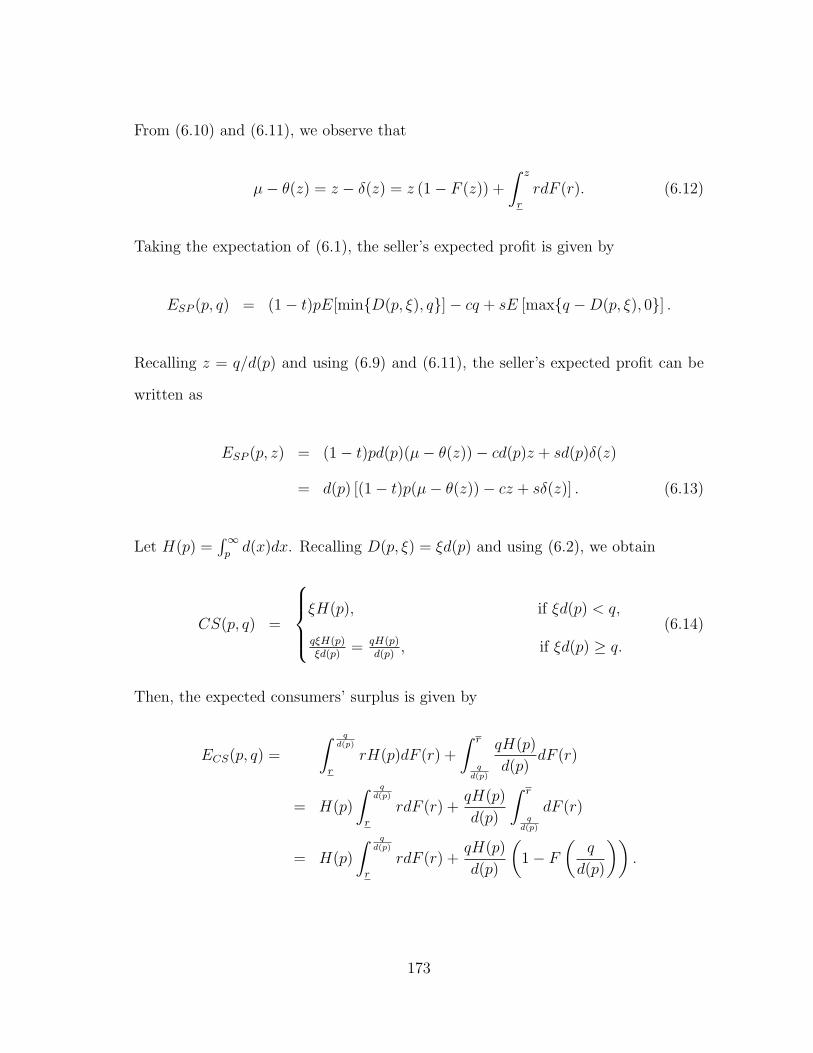
From (6.10) and (6.11), we observe that
µ− θ(z) = z − δ(z) = z (1− F (z)) +
∫ z
r
rdF (r). (6.12)
Taking the expectation of (6.1), the seller’s expected profit is given by
ESP (p, q) = (1− t)pE[min{D(p, ξ), q}]− cq + sE [max{q −D(p, ξ), 0}] .
Recalling z = q/d(p) and using (6.9) and (6.11), the seller’s expected profit can be
written as
ESP (p, z) = (1− t)pd(p)(µ− θ(z))− cd(p)z + sd(p)δ(z)
= d(p) [(1− t)p(µ− θ(z))− cz + sδ(z)] . (6.13)
Let H(p) =∫∞p
d(x)dx. Recalling D(p, ξ) = ξd(p) and using (6.2), we obtain
CS(p, q) =
ξH(p), if ξd(p) < q,
qξH(p)ξd(p)
= qH(p)d(p)
, if ξd(p) ≥ q.
(6.14)
Then, the expected consumers’ surplus is given by
ECS(p, q) =
∫ qd(p)
r
rH(p)dF (r) +
∫ r
qd(p)
qH(p)
d(p)dF (r)
= H(p)
∫ qd(p)
r
rdF (r) +qH(p)
d(p)
∫ r
qd(p)
dF (r)
= H(p)
∫ qd(p)
r
rdF (r) +qH(p)
d(p)
(1− F
(q
d(p)
)).
173

Substituting z = q/d(p) into the above equation and using (6.12), we obtain:
ECS(p, z) = H(p)
∫ z
r
rdF (r) +H(p)z(1− F (z)) = H(p)(µ− θ(z)). (6.15)
By (6.3), the expected externality benefit is given byEEB(p, q) = αE[min{D(p, ξ), q}].
Using z = q/d(p) and (6.11), we obtain
EEB(p, z) = αd(p) (µ− θ(z)) . (6.16)
Due to mathematical ease, in the sequel, we use variables p and z instead of variables
p and q in the analysis.
6.4.2 Comparison between centralized and decentralized decisions
With the explicit expressions for all components in (6.13), (6.15), and (6.16), the
expected social welfare can be written as
ΠC(p, z) = ESP (p, z) + ECS(p, z) + EEB(p, z)
= [(1− t)pd(p) +H(p) + αd(p)] [µ− θ(z)] + (sδ(z)− cz) d(p).(6.17)
In centralized control, the government decides p and z to maximize the expected
social welfare. Hence, the centralized optimization problem is given by
maxp,z
ΠC(p, z).
The socially optimal price p∗C and stocking factor z∗C are presented in Property 1.
Property 1. In centralized control, the optimal retail price p∗C and the stocking factor
174

z∗C that maximize the expected social welfare satisfy
p− td(p)
(1− t)d′(p)
∣∣∣∣p=p∗C
=1
1− t
[c− α +
(c− s)δ(z)
z − δ(z)
]∣∣∣∣z=z∗C
(6.18)
and
F (z∗C) =H(p) + d(p)((1− t)p− c+ α)
H(p) + d(p)((1− t)p− s+ α)
∣∣∣∣p=p∗C
. (6.19)
The optimal order quantity q∗C is given by q∗C = d(p∗C)z∗C.
Proof of Property 1: Recall (6.6) and (6.7) that define θ(z) and δ(z), respectively
and H(p) =∫∞p
d(x)dx. We have H ′(p) = −d(p), θ′(z) = −(1 − F (z)) and δ′(z) =
F (z). Taking the first and second derivatives of ΠC(p, z) in (6.17) w.r.t z, we obtain
∂ΠC(p, z)
∂z= [(1− t)pd(p) +H(p) + αd(p)] [1− F (z)] + sd(p)F (z)− cd(p),(6.20)
and
∂2ΠC(p, z)
∂z2= − [((1− t)p+ α− s) d(p) +H(p)] f(z) < 0,
because p(1−t) ≥ s from Assumption 1 andH(p) > 0 from Assumption 3. Therefore,
ΠC(p, z) is concave in z for any given p and the optimal z satisfies the first order
condition ∂ΠC(p, z)/∂z = 0. In addition, we have
∂ΠC(p, z)
∂p= [(1− t)d(p) + (1− t)pd′(p)− d(p) + αd′(p)] (µ− θ(z))
+(sδ(z)− cz)d′(p), (6.21)
175
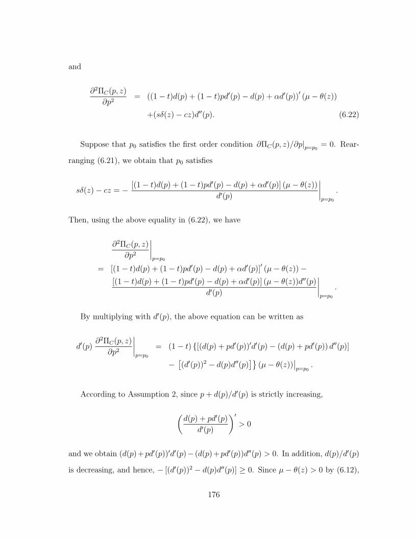
and
∂2ΠC(p, z)
∂p2= ((1− t)d(p) + (1− t)pd′(p)− d(p) + αd′(p))
′(µ− θ(z))
+(sδ(z)− cz)d′′(p). (6.22)
Suppose that p0 satisfies the first order condition ∂ΠC(p, z)/∂p|p=p0= 0. Rear-
ranging (6.21), we obtain that p0 satisfies
sδ(z)− cz = − [(1− t)d(p) + (1− t)pd′(p)− d(p) + αd′(p)] (µ− θ(z))
d′(p)
∣∣∣∣p=p0
.
Then, using the above equality in (6.22), we have
∂2ΠC(p, z)
∂p2
∣∣∣∣p=p0
= [(1− t)d(p) + (1− t)pd′(p)− d(p) + αd′(p)]′(µ− θ(z))−
[(1− t)d(p) + (1− t)pd′(p)− d(p) + αd′(p)] (µ− θ(z))d′′(p)
d′(p)
∣∣∣∣p=p0
.
By multiplying with d′(p), the above equation can be written as
d′(p)∂2ΠC(p, z)
∂p2
∣∣∣∣p=p0
= (1− t) {[(d(p) + pd′(p))′d′(p)− (d(p) + pd′(p)) d′′(p)]
−[(d′(p))2 − d(p)d′′(p)
]}(µ− θ(z))
∣∣p=p0
.
According to Assumption 2, since p+ d(p)/d′(p) is strictly increasing,
(d(p) + pd′(p)
d′(p)
)′
> 0
and we obtain (d(p)+pd′(p))′d′(p)− (d(p)+pd′(p))d′′(p) > 0. In addition, d(p)/d′(p)
is decreasing, and hence, − [(d′(p))2 − d(p)d′′(p)] ≥ 0. Since µ− θ(z) > 0 by (6.12),
176

we have
d′(p)∂2ΠC(p, z)
∂p2
∣∣∣∣p=p0
> 0 and then∂2ΠC(p, z)
∂p2
∣∣∣∣p=p0
< 0.
Hence, ΠC(p, z) is concave at any stationary point p0. Thus, there is a unique
stationary point p0 for a given z which is the optimal price. Dividing both sides of
∂ΠC(p, z)/∂p = 0 by (1− t)d′(p)(µ− θ(z)) (6.21) and using (6.12), we obtain
p− td(p)
(1− t)d′(p)− cz − sδ(z)− α(z − δ(z))
(1− t)(z − δ(z))= 0.
Rearranging the above equation and ∂ΠC(p, z)/∂z = 0 in (6.20), we obtain the
optimal price p∗C and the stocking factor z∗C satisfy (6.18) and (6.19).
Property 1 characterizes the optimal retail price and the order quantity that
maximize the expected social welfare. It is interesting to note that the optimal
solution to the centralized problem given by (6.19) has an elegant form and can be
considered as a generalized solution to the price-setting newsvendor problems with
different objectives. The solution to the profit maximization problem that satisfies
F (z) = (p−c)/(p−s) (see e.g., Nahmias (2005)) can be directly obtained by omitting
consumers’ surplus related term H(p) and letting t = 0 and α = 0 in (6.19). Note
that, in centralized control without the government intervention, the social welfare
incorporates three terms: the seller’s expected profit, the consumers’ surplus, and
the externality benefit. Next property represents the relationship between the three
terms at the socially optimal decisions.
Property 2. In centralized control, ESP (p∗C , z
∗C) ≤ −EEB(p
∗C , z
∗C). More specifically,
1. If t = 0, then ESP (p∗C , z
∗C) = −EEB(p
∗C , z
∗C) and ΠC(p
∗C , z
∗C) = ECS(p
∗C , z
∗C);
and
177

2. If t > 0, then ESP (p∗C , z
∗C) < −EEB(p
∗C , z
∗C), and ΠC(p
∗C , z
∗C) < ECS(p
∗C , z
∗C).
Proof of Property 2: Multiplying both sides of (6.18) by (1− t)d(p)(z− δ(z)) and
rearranging the equation, we have
{(1− t)d(p)p(z − δ(z)) + d(p)(sδ(z)− cz)}|p=p∗C ,z=z∗C
=
{−αd(p)(z − δ(z)) +
td2(p)(z − δ(z))
d′(p)
}∣∣∣∣p=p∗C ,z=z∗C
.
Recall ESP (p, z) and EEB(p, z) from (6.13) and (6.16), respectively, and using z −
δ(z) = µ− θ(z), we observe that
ESP (p∗C , z
∗C) = −EEB(p
∗C , z
∗C) +
td2(p)(z − δ(z))
d′(p)
∣∣∣∣p=p∗C ,z=z∗C
.
Since d′(p) < 0, ESP (p∗C , z
∗C) ≤ −EEB(p
∗C , z
∗C). The equality holds true if t = 0.
Property 2 shows that the seller’s expected profit is non-positive at the socially
optimal decisions. The result directly follows from ESP (p∗C , z
∗C) ≤ −EEB(p
∗C , z
∗C) and
the expected externality benefit EEB(p, z) = αd(p) (µ− θ(z)) is always nonnegative
due to α > 0. Hence, the more beneficial the public interest product is to the
community, the more loss the seller faces. It is interesting to note that when the
tax rate is zero, the absolute values of the seller’s expected profit and the expected
externality benefit are equal, and hence, the expected social welfare is equal to the
expected consumers’ surplus.
In decentralized control, the seller maximizes the expected profit without consid-
ering the consumers’ surplus and the externality benefit. Using (6.13), the decen-
tralized optimization problem is given by
maxp,z
ΠD(p, z) = maxp,z
ESP (p, z) = maxp,z
d(p) [(1− t)p(µ− θ(z))− cz + sδ(z)] . (6.23)
178

The optimal price p∗D and the stocking factor z∗D in decentralized control are presented
in the following property.
Property 3. In decentralized control, the optimal retail price p∗D and the stocking
factor z∗D that maximize the seller’s expected profit satisfy
p+d(p)
d′(p)
∣∣∣∣p=p∗D
=1
1− t
[c+
(c− s)δ(z)
z − δ(z)
]∣∣∣∣z=z∗D
and
F (z∗D) =(1− t)p− c
(1− t)p− s
∣∣∣∣p=p∗D
. (6.24)
The optimal order quantity q∗D is given by q∗D = d(p∗D)z∗D.
Proof of Property 3: Taking the first and second derivatives of ΠD(p, z) in (6.23)
with respect to z and using θ′(z) = −[1− F (z)] and δ′(z) = F (z), we obtain
∂ΠD(p, z)
∂z= (1− t)pd(p)[1− F (z)] + sd(p)F (z)− cd(p), (6.25)
and
∂2ΠD(p, z)
∂z2= −(1− t)pd(p)f(z) + sd(p)f(z)
= − [(1− t)p− s] d(p)f(z) ≤ 0,
because (1 − t)p ≥ s from Assumption 1. Next, we analyze two possible cases,
respectively, when (1− t)p = s and (1− t)p > s. If (1− t)p = s, ∂2ΠD(p, z)/∂z2 = 0
and ΠD(p, z) is decreasing in z, because ∂ΠD(p, z)/∂z = (s − c)d(p) < 0 from
Assumption 1. Hence, ΠD(p, z) achieves its optimal value at z = 0. In this case, the
179

seller’s expected profit is zero such that
ΠD(p, z)|z=0 = d(p) [(1− t)p(µ− θ(z))− cz + sδ(z)] |z=0 = 0.
However, it cannot be the optimal solution, because there exists at least one feasible
solution that leads to a profit. Since (1− t)p > c from Assumption 1, there exists a
feasible retail price p∗, s.t. p∗ ∈ (c/(1− t), p). Let z∗ = r. Then, the expected profit
function at the feasible solution (p∗, z∗) is positive, which is given by
ΠD(p, z)|p=p∗,z=z∗ = d(p) [(1− t)pz − cz] |p=p∗,z=z∗ > 0.
Therefore, the optimal solution of ΠD(p, z) cannot be achieved when (1 − t)p = s.
The optimal retail price should satisfy (1 − t)p > s. For any given p in the range
(1 − t)p > s, ΠD(p, z) is strictly concave in z and the optimal z satisfies the first
order condition ∂ΠD(p, z)/∂z = 0. In addition, we have
∂ΠD(p, z)
∂p= (1− t) (µ− θ(z)) (d(p) + pd′(p)) + (sδ(z)− cz)d′(p), (6.26)
and
∂2ΠD(p, z)
∂p2= (1− t) (µ− θ(z)) [d′(p) + d′(p) + pd′′(p)] + (sδ(z)− cz)d′′(p).
= (1− t) (µ− θ(z)) [2d′(p) + pd′′(p)] + (sδ(z)− cz)d′′(p). (6.27)
Suppose that p0 satisfies the first order condition ∂ΠD(p, z)/∂p|p=p0= 0. Rearrang-
ing (6.26), we obtain that p0 satisfies
sδ(z)− cz = − (1− t)(µ− θ(z)) [d(p) + pd′(p)]
d′(p)
∣∣∣∣p=p0
.
180

Then, using the above equality in (6.27) and multiplying both sides with d′(p), we
have
∂2ΠD(p, z)
∂p2
∣∣∣∣p=p0
= (1− t) (µ− θ(z)) [2d′(p) + pd′′(p)]
− (1− t)(µ− θ(z)) [d(p) + pd′(p)] d′′(p)
d′(p)
∣∣∣∣p=p0
.
According to Assumption 2, since p+ d(p)/d′(p) is strictly increasing,
(d(p) + pd′(p)
d′(p)
)′
> 0
and we obtain [2d′(p) + pd′′(p)] d′(p)−(d(p)+pd′(p))d′′(p) = 2[d′(p)]2−d(p)d′′(p) > 0.
Therefore, we have
d′(p)∂2ΠD(p, z)
∂p2
∣∣∣∣p=p0
> 0, and∂2ΠD(p, z)
∂p2
∣∣∣∣p=p0
< 0.
Hence, ΠD(p, z) is concave at any stationary point p0. Thus, there is a unique
stationary point of ΠD(p, z) w.r.t p for a given z which is the optimal price.
Dividing both sides of ∂ΠD(p, z)/∂p = 0 by (1− t)d′(p)(µ− θ(z)) given in (6.26)
and using (6.12), we obtain
p+d(p)
d′(p)− cz − sδ(z)
(1− t)(µ− θ(z))= p+
d(p)
d′(p)− cz − sδ(z)
(1− t)(z − δ(z))= 0.
Rearranging the above equation and using ∂ΠD(p, z)/∂z = 0 given by (6.25), we
obtain that the optimal price p∗D and the stocking factor z∗D satisfy
p+d(p)
d′(p)
∣∣∣∣p=p∗D
=1
1− t
[c+
(c− s)δ(z)
z − δ(z)
]∣∣∣∣z=z∗D
and F (z∗D) =(1− t)p− c
(1− t)p− s
∣∣∣∣p=p∗D
.
181

Due to the impact of consumers’ surplus and externality benefit, the optimal
decisions are different under the two objectives. Property 4 provides the comparison
between the socially optimal decisions and the decentralized optimal decisions.
Property 4. p∗C < p∗D, z∗C > z∗D, and q∗C > q∗D.
Proof of Property 4: In Properties 1 and 3, we prove that p∗C and z∗C satisfy the
first order conditions of ΠC(p, z), and p∗D and z∗D satisfy the first order conditions of
ΠD(p, z). Using (6.21), we have
∂ΠC(p, z)
∂p
∣∣∣∣p=p∗C ,z=z∗C
= {[(1− t)d(p) + (1− t)pd′(p)− d(p) + αd′(p)] (µ− θ(z))
+(sδ(z)− cz)d′(p)}|p=p∗C ,z=z∗C= 0. (6.28)
From (6.26), we have
∂ΠD(p, z)
∂p
∣∣∣∣p=p∗C ,z=z∗C
= {d′(p) [(1− t)p(µ− θ(z))− cz + sδ(z)]
+(1− t)d(p) (µ− θ(z))}|p=p∗C ,z=z∗C
=
{∂ΠC(p, z)
∂p+ d(p)(µ− θ(z))− αd′(p) (µ− θ(z))
}∣∣∣∣p=p∗C ,z=z∗C
= {d(p)(µ− θ(z))− αd′(p) (µ− θ(z))}|p=p∗C ,z=z∗C.
According to (6.11) and Assumption 2, the first term d(p)(µ − θ(z)) represents the
expected sales, which should be positive, as well as (µ− θ(z)) > 0 and d′(p) < 0. We
obtain ∂ΠD(p, z)/∂p|p=p∗C ,z=z∗C> 0. Hence, p∗D > p∗C .
182

Using (6.20) and (6.25), and the definitions of p∗D and z∗D, we obtain
∂ΠC(p, z)
∂z
∣∣∣∣p=p∗D,z=z∗D
= {(1− t)pd(p)[1− F (z)]
+ sd(p)F (z)− cd(p) + [H(p) + αd(p)][1− F (z)]}|p=p∗D,z=z∗D
=∂ΠD(p, z)
∂z
∣∣∣∣p=p∗D,z=z∗D
+ {[H(p) + αd(p)] [1− F (z)]}|p=p∗D,z=z∗D
= { [H(p) + αd(p)] [1− F (z)]}|p=p∗D,z=z∗D> 0.
Hence, z∗C > z∗D. Furthermore, q∗C = z∗Cd(p∗C) > z∗Dd(p
∗D) = q∗D.
Property 4 demonstrates that the seller’s decentralized optimal retail price is
higher and the order quantity is lower than the corresponding socially optimal de-
cisions. In other words, in centralized control, a lower price is charged and more
quantity is obtained in order to transfer a part of the seller’s profit to consumers to
improve the expected social welfare. These results are consistent with our intuition,
as consumers always prefer a lower retail price and more quantity available in the
market.
6.5 Intervention mechanisms
We have already shown in Property 4 that the seller’s decisions are not socially
optimal in a free market (i.e., in decentralized control). The question arises how
the government intervenes in the market to align the seller’s decisions with the so-
cially optimal ones. In this section, we examine several government intervention
mechanisms and investigate their coordination performance and efficiency. The gov-
ernment intervention mechanisms of interest are illustrated in Figure 6.2. The regu-
latory mechanisms and market mechanisms will be discussed in Sections 6.1 and 6.2,
respectively.
183

GovernmentInterventions
The retailer decides
p, q,
D(p) = ξ d(p)
Maximum price
Minimum quantity
Tax cut
Consumer rebate
Cost subsidy
Regularity Interventions
Market Interventions
Figure 6.2: The framework of government intervention mechanisms.
We will evaluate and compare these government interventions from three aspects:
the effectiveness, coordination efficiency, and the government cost. With the effec-
tiveness of an intervention, we pay attention to whether the socially optimal price,
stocking factor, and/or quantity can be achieved through the intervention. With co-
ordination efficiency of an intervention, we are interested in the following questions:
a) does the intervention lead to a better expected social welfare, and b) how close is
it to the socially optimal expected welfare? Besides coordination efficiency, the gov-
ernment cost is also a critical concern when the government chooses an intervention
from multiple options. Hence, the cost should be taken into account for intervention
evaluation.
6.5.1 Regulatory intervention mechanisms
As discussed previously, regulatory interventions are often implemented by the
government to improve social welfare. As shown in Figure 6.2, we consider three gov-
ernment regulations such as maximum price regulation (i.e., the government restricts
184

the highest retail price to p∗C), minimum quantity regulation (i.e., the government
restricts the lowest order quantity to q∗C), and maximum price and minimum quan-
tity regulation (i.e., the government restricts the highest retail price to p∗C and lowest
order quantity to q∗C). It is worth noting that it is possible for the government to
enforce the seller to sell the product at or below a given price under the maximum
price regulation only when the seller’s expected profit is positive at the price; other-
wise, the seller would exit the market. When the demand function is additive (i.e.,
D(p, ξ) = ξ+d(p)), according to (6) in Ovchinnikov and Raz (2014), the socially op-
timal price is c−α−Θ(z∗C)/2. This price is less than c, since the constant marginal
benefit α > 0 and the expected shortage Θ(z∗C) ≥ 0. In this case, the maximum
price regulation will be ruled out, because the seller does not make a profit by sell-
ing the product. However, when the demand function is multiplicative, the socially
optimal retail price might be more than the production/ordering cost after tax, i.e.,
p∗C > c/(1− t).
The explanation for the different results is the following. Recall that E(ξ) = µ
and var(ξ) = σ2. For the additive demand function, the variance is var(D(p, ξ)) =
var(ξ+d(p)) = σ2, and the coefficient of variation is CV (D(p, ξ)) = CV (ξ+d(p)) =
σd(p)/(d(p) + µ). Therefore, the variance of the additive demand function is con-
stant in p while the coefficient of variation increases in p. On the other hand,
for the multiplicative demand function, var(D(p, ξ)) = var(ξd(p)) = d2(p)σ2 and
CV (D(p, ξ)) = CV (ξd(p)) = σ/µ. That is, the variance of the multiplicative demand
function decreases in p and the corresponding coefficient of variation is constant in p.
Note that both variance and coefficient of variation measure extents of variabilities
of demands and they are expected to be low. Hence, in the additive case, a lower
price is charged to decrease coefficient of variation, while in the multiplicative case, a
higher price is charged to decrease variance to reduce the demand uncertainty. The
185

following property presents a condition that ensures p∗C > c/(1− t).
Property 5. If
td(p)
d′(p)
∣∣∣∣p=p∗C
+(c− s)δ(z)
z − δ(z)
∣∣∣∣∣z=z∗C
− α > 0, (6.29)
then p∗C > c/(1− t).
The proof of Property 5 follows by rearranging (6.18). Note that inequality
(6.29) is obviously satisfied when the sales tax t is zero, and the constant marginal
externality α is less than a threshold value, such as
α <(c− s)δ(z)
z − δ(z)
∣∣∣∣z=z∗C
.
Thus, if α and t are small enough, the condition in Property 5 holds true, and
hence, the maximum price regulation is effective to coordinate the price. Recall that
a higher constant marginal externality α implies that more benefit is generated to the
community from purchasing the product by a consumer. If the benefit is high for a
product, then the goal of maximizing the expected social welfare should be achieved
through lowering the price, increasing the affordability, and popularizing the product.
In this case, the socially optimal price may be very low so that p∗C ≤ c/(1− t). Prop-
erty 5 reveals scenarios where it is possible for the seller to have a positive expected
profit under the mandatory maximum price p∗C . Hence, the regulatory intervention
on price is effective to coordinate the price for the multiplicative demand function for
some cases. It is a significantly different result from the additive case. The following
property shows the seller’s optimal decisions under the three regulations.
Property 6. 1. Under the maximum price regulation, the seller’s optimal price
p∗MP is the socially optimal price p∗MP = p∗C, and the optimal stocking factor
186

z∗MP satisfies
F (z∗MP ) =(1− t)p∗C − c
(1− t)p∗C − s. (6.30)
We have
z∗MP < z∗D < z∗C , and q∗MP < q∗C .
2. Under the minimum quantity regulation, the seller’s optimal quantity q∗MQ is the
socially optimal quantity q∗MQ = q∗C, and the optimal retail price p∗MQ satisfies
p
∫ q/d(p)
rrdF (r)
q/d(p)− δ(q/d(p))
+d(p)
d′(p)
∣∣∣∣∣∣p=p∗MQ,q=q∗C
=s
1− t
∫ q/d(p)
rrdF (r)
q/d(p)− δ(q/d(p))
∣∣∣∣∣∣p=p∗MQ,q=q∗C
.
We have
p∗MQ > p∗C , and z∗MQ =q∗C
d(p∗MQ)> z∗c > z∗D.
3. Under the maximum price and minimum quantity regulation, the seller’s opti-
mal quantity is q∗MPQ = q∗C, and the optimal retail price p∗MPQ = p∗C.
Proof of Property 6:
1. Under the maximum price regulation, the seller’s price p is restricted by the
constraint p ≤ p∗C . From Property 4, we have p∗D > p∗C . Hence, the seller’s optimal
price, p∗MP , under the maximum price regulation is binding at the constraint such
that p∗MP = p∗C . We also know that, from Property 3, for a given p, the decentralized
optimal stocking factor satisfies the first order condition ∂ΠD(p, z)/∂z = 0. Then,
for given p = p∗C , using (6.25), the optimal stocking factor z∗MP under the maximum
187
price regulation satisfies
∂ΠD(p, z)
∂z
∣∣∣∣p=p∗C ,z=z∗MP
= {[(1− t)p [1− F (z)] + sF (z)− c]d(p)}|p=p∗C ,z=z∗MP= 0.
Thus, we have (6.30). Recall p∗C < p∗D and z∗D > z∗C from Property 4. Using (6.24),
we have F (z∗MP ) < F (z∗D). Then, we have z∗MP < z∗D < z∗C and q∗MP < q∗C , since
q∗MP = d(p∗MP )z∗MP = d(p∗C)z
∗MP < d(p∗C)z
∗C = q∗C with p∗MP = p∗C .
2. Under the minimum quantity regulation, the seller’s order quantity q is re-
stricted by the constraint q ≥ q∗C . We will first prove that the decentralized optimal
price satisfies the first order condition ∂ΠD(p, q)/∂q = 0, for a given q. Then, we
will show that the centralized optimal price also satisfies the first order condition
∂ΠC(p, q)/∂q = 0 for a given q, and compare the price decisions under the two situ-
ations. The objective function under the decentralized control can be expressed by
p and q as below
ΠD(p, q) = [(1− t)pd(p)] [µ− θ(q/d(p))] + sd(p)δ(q/d(p))− cq, (6.31)
which is obtained by substituting z = q/d(p) into (6.23). The decentralized problem
in (6.31) is the typical price-setting newsvendor problem with multiplicative demand
excepted that the sales revenue is taxed by t. The typical newsvendor problem is
investigated by Song et al. (2009). They show, in Proposition 1 of their work, that
there is a unique price that maximizes the objective function for a given quantity,
and the objective function all about quantity is concave under specific assumptions.
Incorporating the tax in our model, we are still able to prove the same result following
the proof of Proposition 1 of Song et al. (2009). To avoid repetition, we use the
result directly and inherit their assumptions, which are Assumptions 2 and 3 in this
188

chapter. We conclude that, for any given q, the optimal price p to ΠD(p, q) in (6.31)
satisfies the first order condition ∂ΠD(p, q)/∂p = 0, and ΠD(p(q), q) is concave in q,
under Assumptions 2 and 3, where p(q) is the optimal price given q. Recall q∗D < q∗C
from Properties 4. The seller’s optimal quantity q∗MQ under the minimum quantity
regulation is binding at the constraint such that q∗MQ = q∗C . The optimal price p∗MQ
satisfies ΠD(p, q)/∂p|p=p∗MQ,q=q∗C= 0 given q = q∗C . We will characterize the relation
of p∗MQ and q∗C next. Differentiating (6.31) with respect to p, we have
ΠD(p, q)
∂p= [(1− t)d(p) + (1− t)pd′(p)] [µ− θ(q/d(p))] + sd′(p)δ(q/d(p))
−(1− t)p[1− F (q/d(p))]qd′(p)
d(p)− sF (q/d(p))
qd′(p)
d(p). (6.32)
Recall that substituting z = q/d(p) into (6.12) gives
[1− F (q/d(p))]q/d(p) = q/d(p)− δ(q/d(p))−∫ q/d(p)
r
rdF (r). (6.33)
Dividing both sides of (6.32) by (1− t)d′(p)[µ− θ(q/d(p))] and using (6.33), we have
ΠD(p,q)∂p
(1− t)d′(p)[µ− θ(q/d(p))]= p
∫ q/d(p)
rrdF (r)
q/d(p)− δ(q/d(p))
+d(p)
d′(p)
− s
1− t
∫ q/d(p)
rrdF (r)
q/d(p)− δ(q/d(p))
.
Recalling ΠD(p, q)/∂p|p=p∗MQ,q=q∗C= 0 and using the above equation after some alge-
189

bra, we have
p
∫ q/d(p)
rrdF (r)
q/d(p)− δ(q/d(p))
+d(p)
d′(p)
∣∣∣∣∣∣p=p∗MQ,q=q∗C
=s
1− t
∫ q/d(p)
rrdF (r)
q/d(p)− δ(q/d(p))
∣∣∣∣∣∣p=p∗MQ,q=q∗C
. (6.34)
Now, we have found the relation of p∗MQ and q∗C . To compare p∗MQ and p∗C , we need
to identify the relation of p∗C and q∗C . In the centralized problem, the expected social
welfare function, ΠC(p, q) expressed in p and q, can be obtained by substituting
z = q/d(p) into ΠC(p, z) from (6.17). The expected social welfare function is then
given by
ΠC(p, q) = [(1− t)pd(p) +H(p) + αd(p)] [µ− θ(q/d(p))] + sd(p)δ(q/d(p))− cq.
First, we prove that for any given q, for q > 0, there exits a p(q) that satisfies the
first order condition:
∂ΠC(p, q)
∂p
∣∣∣∣p=p(q)
= 0.
For a given q, the first derivative of ΠC(p, q) with respect to p is given by
∂ΠC(p, q)
∂p= [(1− t)p+ α− s] d′(p)
∫ q/d(p)
r
rdF (r)− td(p)[µ− θ(q/d(p))]
−H(p)
d(p)d′(p)
[µ− θ(q/d(p))−
∫ q/d(p)
r
rdF (r)
]. (6.35)
Then, we prove by contradiction that there exists at least one p that satisfies ΠC(p, q)/∂p =
190

0 for a given q. Suppose that there exists a q0, such that
∂ΠC(p, q0)
∂p> 0,
for ∀p ∈ [s/(1− t), p]. Then, the optimal price is achieved at the upper bound p = p,
where d(p) = 0 defined in Assumption 1. In this case, the expected sales is zero,
and the revenue only comes from salvaging the order quantity. The expected profit
is ΠC(p, q0) = (s − c)q0 < 0, since s < c from Assumption 1. Thus, the solution
{p, q0} is not possible to be optimal. Suppose that these exists a q0, such that
∂ΠC(p, q0)/∂p < 0 for ∀p ∈ [s/(1− t), p]. Then, the optimal price is achieved at the
lower bound p = max{s/(1− t), d−1 (q0/r)}. It does not make sense to set the price
too low that the minimum possible demand is greater than the given quantity. So we
need rd(p) ≥ q0, equivalent to p ≥ d−1 (q0/r). For the case that s/(1−t ≥ d−1 (q0/r)),
the lower bound is p = s/(1 − t). Then, the seller’s revenue after tax is the salvage
value, and hence, the expected profit is (s− c)q0 < 0. So p = s/(1− t) cannot be the
optimal decision. For the other case that d−1 (q0/r) > s/(1 − t), we have the lower
bound p(q0) = d−1 (q0/r) and q0/d(p(q0)) = r.
Substituting z = q/d(p) into (6.16), we have EEB(p, q0) = H(p)(µ− θ(q0/d(p))).
191

Differentiating the sum of (6.15) and the above equation with respect to p gives
limp→p(q0)
∂[ECS(p, q0) + EEB(p, q0)]
∂p
= limp→p(q0)
{[−d(p) + αd′(p)] (µ− θ(q0/d(p)))}
+ limp→p(q0)
{[H(p) + αd(p)] (F (q0/d(p))− 1)
q0/d(p)d′(p)
d(p)
}= lim
p→p(q0)
{−q0/d(p)
d′(p)
d(p)H(p) + αd′(p)
∫ q0/d(p)
r
rdF (r)− q0
}
= limp→p(q0)
−q0/d(p)d′(p)
d(p)H(p)− q0 > −∞.
Furthermore, substituting z = q/d(p) into (6.13) and using results in Proposition
1 of Song et al. (2009), we can easily derive that
limp→p(q0)
∂ESP (p, q0)
∂p= ∞.
Then,
limp→p(q0)
∂ΠC(p, q0)
∂p= lim
p→p(q0)
∂ΠSP (p, q) + ΠCS(p, q) + ΠEB(p, q)
∂p> 0,
which contradicts ∂ΠC(p, q0)/∂p < 0. Thus, there exists at least one p ∈ [s/(1−t), p]
satisfying ∂ΠC(p, q)/∂p = 0 for a given q. As we already prove that the optimal
price does not occur at the boundary points, the optimal price p∗C should satisfy
the first order condition, ∂ΠC(p, q)/∂p|p=p∗C ,q=q∗C= 0, at the order quantity q = q∗C .
Substituting µ − θ(q/d(p)) = q/d(p) − δ(q/d(p)) from (6.33) into (6.35) and using
(6.34), when the optimal decision {p = p∗MQ, q = q∗C} under the minimum quantity
192

regulation is used, we obtain
∂ΠC(p, q)
∂p
∣∣∣∣p=p∗MQ,q=q∗C
=1
1− td′(p)[q/d(p)− δ(q/d(p))] · α
∫ q/d(p)
rrdF (r)
q/d(p)− δ(q/d(p))− d(p)
d′(p)+
H(p)
d(p)
1−∫ q/d(p)
rrdF (r)
q/d(p)− δ(q/d(p))
∣∣∣∣∣∣p∗MQ,q∗C
.
From (6.12), we have q/d(p)−δ(q/d(p))−∫ q/d(p)
rrdF (r) > 0, and hence, the last term
of the above equation is positive. Recall d′(p) < 0. We have ∂ΠC(p, q)/∂p|p=p∗MQ,q=q∗C<
0. Recalling ∂ΠC(p, q)/∂p|p=p∗C ,q=q∗C= 0, we conclude p∗C < p∗MQ and z∗MQ =
q∗C/d(p∗MQ) > z∗C > z∗D.
3. Under both maximum price and minimum quantity regulations, when both
constraints p ≤ p∗C and q ≥ q∗C are applied, the optimal retail price p∗B and quantity
q∗B are binding at q∗B = q∗C and p∗B = p∗C , because q∗MP < q∗C and p∗MQ > p∗C .
There are several implications about the regularity interventions discussed in
Property 6. First, if the government sets the highest retail price to the socially
optimal price, then the seller would charge the socially optimal price and order less
than the socially optimal quantity. Second, if the government regulates the lowest
quantity as the socially optimal quantity, then the seller would order the socially
optimal quantity and charge a price higher than the socially optimal price. Third,
if the government regulates both the highest price and the lowest quantity, then
the seller uses the socially optimal decisions. However, from Property 2, we know
that the seller’s expected profit is non-positive if the socially optimal price and the
order quantity are used. Hence, the third regulation is not applicable in a real-world
situation. In addition, note that p∗C > c/(1 − t) is not a sufficient condition for the
seller to have a positive expected profit. If the order quantity is required to be high
(i.e., under the minimum quantity regulation) and any leftover is sold at a salvage
193

value s < c, then a loss may occur for the seller. Hence, similar to the maximum price
regulation, the minimum quantity regulation is also only applicable when the seller
have a positive expected profit. Otherwise, if the government intends to practice
such regulations that result in a loss, the government has to compensate the seller
for the expected profit loss.
6.5.2 Market intervention mechanisms
Although it is possible for the maximum price and minimum quantity regulations
to coordinate the retail price and the order quantity, respectively, the regulations suf-
fer from several limitations. First, a regulation is not effective for coordination when
the seller’s expected profit is non-positive. Second, an effective regulation, i.e., the
maximum price or minimum quantity regulation, cannot align the seller’s both de-
cisions simultaneously. Third, there is little flexibility for the seller in choosing the
price/quantity decision, under the regulation restricting price/quantity. The inflex-
ibility may eliminate the seller’s incentive to collaborate with the government and
continue the business to sell a public interest good in long term. To address these
problems, in this section, we investigate three market intervention mechanisms, in-
cluding tax cut, consumer rebate, and cost subsidy mechanisms, and their combina-
tions. We characterize the seller’s and consumers’ behaviors under the interventions
and identify the interventions’ effectiveness and efficiency of coordination.
In the sequel, we will first introduce the three market interventions. Then, we
derive expressions for the seller’s expected profit and the government’s expected cost
for a generalized case where all three market interventions are applied. Given the
general expressions, formulas for each special case, where only one or two of the three
market interventions are applied, can be identified easily.
194

6.5.2.1 Tax cut
Tax cut is reduction in taxes. It usually serves as an important intervention im-
plemented by the government to leverage price and stimulate sales for a product (see
e.g., Dardan and Stylianou (2000)). Under the tax cut intervention, the government
imposes a lower tax rate T on the product than the original rate t. Note that, to
increase the flexibility of the mechanism, we do not restrict the new tax rate T on a
positive range, and we allow for the tax rate reduced to a negative value. In this case,
the government pays money back instead of charging a tax to the seller to stimulate
the seller to make the socially optimal decisions. The tax cut would increase the
seller’s profit with no raise in the retail price. Hence, the government’s expected rev-
enue is decreased, while the seller’s revenue from selling a unit product is expected
to rise. It gives the seller an incentive to sell more by ordering more quantity and/or
charging a lower price. Under the tax cut mechanism, the seller’s expected profit
function is the same as (6.13) except using the new tax rate T instead of t.
6.5.2.2 Consumer rebate
A consumer rebate is a payment transferred from the government to a consumer
for each unit that the consumer purchases, with the intention of increasing the af-
fordability of the product. The common types of rebates include cash back, vouchers,
and coupons. In this chapter, we assume that cash back is used. Let R denote the
consumer rebate per unit. Let p′ be the retail price the seller charges and p be the
effective price that consumers actually pay for the product after the rebate. Hence,
we have p = p′ − R. With rebates, the product is expected to be affordable to
more consumers. This intervention provides an incentive for the seller to order more
quantity or charge a lower price to satisfy more consumers. For the notational and
computational convenience, we model the seller’s behavior using the effective price
195

p, instead of the seller’s price p′, because it is the effective price that determines the
amount of demand. In particular, with rebates, the seller’s revenue per unit sold
is p′ = p + R. Hence, the seller’s expected profit with rebates ESP (p, z, R) can be
obtained by (6.13) by replacing p with p + R for the seller’s revenue per unit sold
given by
ΠR(p, z) = d(p) [(1− t)(p+R)(µ− θ(z))− cz + sδ(z)] . (6.36)
It is interesting to note that the consumer rebate intervention is equivalent to
another intervention, which we call “the seller rebate intervention”. Under the seller
rebate intervention, the rebate R is given to the seller as a cash back for each unit
sold, instead of the consumer. Taking p as the price charged to consumers and p+R
as the seller’s revenue per unit sold, the seller’s expected profit is the same as the
one in (6.36) and the expected government cost also remains unchanged. In this
sense, these two intervention mechanisms, the consumer rebate and the seller rebate,
are equivalent. The seller rebate intervention is also similar to the sales subsidy
intervention considered by Taylor and Yadav (2011), under which the donor pays
the sales subsidy to the retailer.
6.5.2.3 Cost subsidy
The cost subsidy is a payment transferred from the government to the seller for
each unit the seller purchases or produces, with the intention of inducing the seller
to keep more quantity and charge a less retail price. Suppose the cost subsidy is
denoted by S. The cost subsidy given to the seller decreases the effective purchase
or production/ordering cost from c to c − S. Note that, with subsidies, the seller’s
optimization problem is equivalent to the decentralized problem given by (6.13) with
production/ordering cost c− S. Thus, c− S > s is required in practice. Otherwise,
196

if c−S ≤ s, the seller would order as much as possible because the seller can always
make a profit by salvaging the leftovers.
Although the three interventions provide different incentives, all of them can be
considered as mechanisms to compensate the seller in different ways. In particular,
S is the compensation paid by the government to the seller for each product ordered,
R is the compensation paid by the government to the seller for each product sold,
and tax difference t− T is the compensation paid by the government for each dollar
earned by the seller.
6.5.2.4 Generalized expressions for intervention mechanisms
Next, we investigate a combination of the three interventions and derive the
expressions for the seller’s expected profit and the government’s expected cost when
the combination is applied.
Suppose that the government executes tax cut, consumer rebate, and cost subsidy
intervention mechanisms at the same time: a new tax rate T is charged to the seller,
a consumer rebate R is applied on each unit sold to consumers, and a cost subsidy S
is applied on each unit ordered to the seller. Then, the seller’s cost per unit ordered
is reduced from c to c − S, and the seller’s revenue per unit sold is increased from
p to p + R, recalling that, p refers to the effective price after the rebate. Hence, by
replacing c with c−S for the seller’s unit cost, replacing p with p+R for the seller’s
unit revenue, and replacing the original tax rate t with the new tax rate T in the
seller’s expected profit function given by (6.13), we obtain the seller’s expected profit
under the combination of the three market interventions as below:
ESP (p, z, T, R, S) = d(p) [(1− T )(p+R)(µ− θ(z))− (c− S)z + sδ(z)] .(6.37)
Meanwhile, the expected revenue of the government is reduced due to the de-
197
creased tax revenue, the rebates paid to all customers purchasing the product, and
the subsidies paid to the seller for ordered units. The government’s expected cost,
EGC(p, z, T, R, S), is measured as the difference between the government’s expected
revenues without and with the interventions. Without the interventions, the govern-
ment’s expected revenue, the tax rate times the seller’s expected revenue (see (6.11)),
is given by
tpd(p)(µ− θ(z)). (6.38)
The government pays a subsidy to the seller for each unit the seller orders. The
payment is given by
Szd(p) (6.39)
where q = zd(p) is the seller’s order quantity. The government also pays rebates
to all consumers who purchase the product. The expected payment is R times the
seller’s expected sales (see (6.11)) given by
Rd(p)(µ− θ(z)). (6.40)
Furthermore, the government’s expected tax revenue with the tax rate T is
T (p+R)d(p)(µ− θ(z)). (6.41)
Thus, the government’s expected revenue under the interventions is the expected tax
revenue net the expected costs on subsidies and rebates in (6.41), (6.39), and (6.40),
respectively, given by
T (p+R)d(p)(µ− θ(z))−Rd(p)(µ− θ(z))− Szd(p). (6.42)
198
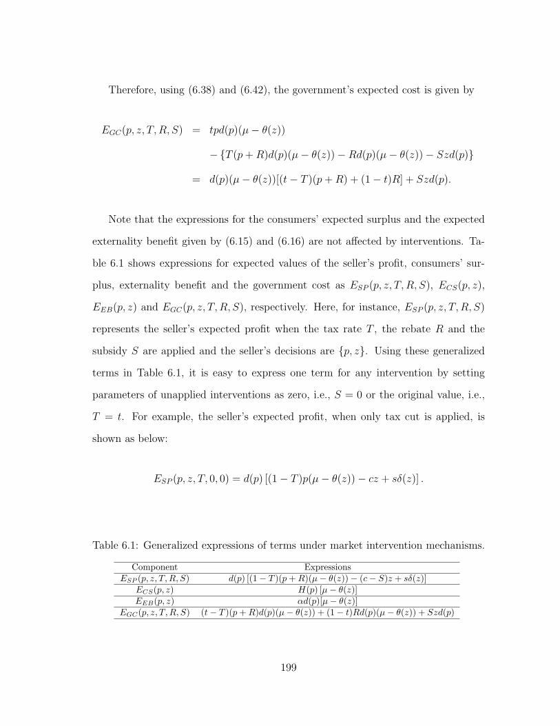
Therefore, using (6.38) and (6.42), the government’s expected cost is given by
EGC(p, z, T, R, S) = tpd(p)(µ− θ(z))
−{T (p+R)d(p)(µ− θ(z))−Rd(p)(µ− θ(z))− Szd(p)}
= d(p)(µ− θ(z))[(t− T )(p+R) + (1− t)R] + Szd(p).
Note that the expressions for the consumers’ expected surplus and the expected
externality benefit given by (6.15) and (6.16) are not affected by interventions. Ta-
ble 6.1 shows expressions for expected values of the seller’s profit, consumers’ sur-
plus, externality benefit and the government cost as ESP (p, z, T,R, S), ECS(p, z),
EEB(p, z) and EGC(p, z, T, R, S), respectively. Here, for instance, ESP (p, z, T,R, S)
represents the seller’s expected profit when the tax rate T , the rebate R and the
subsidy S are applied and the seller’s decisions are {p, z}. Using these generalized
terms in Table 6.1, it is easy to express one term for any intervention by setting
parameters of unapplied interventions as zero, i.e., S = 0 or the original value, i.e.,
T = t. For example, the seller’s expected profit, when only tax cut is applied, is
shown as below:
ESP (p, z, T, 0, 0) = d(p) [(1− T )p(µ− θ(z))− cz + sδ(z)] .
Table 6.1: Generalized expressions of terms under market intervention mechanisms.
Component ExpressionsESP (p, z, T,R, S) d(p) [(1− T )(p+R)(µ− θ(z))− (c− S)z + sδ(z)]
ECS(p, z) H(p) [µ− θ(z)]EEB(p, z) αd(p)[µ− θ(z)]
EGC(p, z, T,R, S) (t− T )(p+R)d(p)(µ− θ(z)) + (1− t)Rd(p)(µ− θ(z)) + Szd(p)
199

For presentational convenience, we use (T,R, S) to represent an intervention when
the tax rate T , the cost subsidy S, and the consumer rebate R are applied. Specif-
ically, (T, 0, 0), (t, R, 0), and (t, 0, S) present the tax cut, the rebate, and the sub-
sidy interventions, respectively, where t is the original tax rate. Similarly, (T,R, 0),
(T, 0, S), and (t, R, S) represent the joint tax-rebate, the joint tax-subsidy, and the
joint rebate-subsidy mechanisms, respectively.
6.5.3 Coordination performance under market intervention mechanisms
As mentioned earlier in Section 6.5.2, intervention parameters T , R , and S cannot
be chosen arbitrarily. That is, the compensation by the government cannot be set so
unrewarding or rewarding that the seller’s decision is always to order nothing or to
order as much as possible under an intervention. We know that, for the cost subsidy,
c− S > s is required. It is also natural to assume that the seller’s revenue per unit
sold after rebate and tax cut is equal to or greater than the salvage value, so that
(1− T )(p+R) ≥ s holds. The conditions that ensure a meaningful intervention are
summarized in Assumption 4.
Assumption 4. 1. The seller’s cost after cost subsidy is greater than the salvage
value, i.e., c− S > s.
2. The seller’s revenue after rebate and tax cut is greater than the salvage value,
i.e., (1− T )(p+R) > s for p ≤ p.
Property 7 characterizes the seller’s optimal price and the optimal stocking factor
under a combination of interventions, when Assumption 4 is satisfied.
Property 7. Under an intervention mechanism L = (T,R, S), where T , R, and
S satisfy Assumption 4, the optimal retail price p∗L and the stocking factor z∗L that
200

maximize the seller’s expected profit satisfy
p+R +d(p)
d′(p)
∣∣∣∣p=p∗L
=1
1− T
[(c− S) +
(c− S − s)δ(z)
z − δ(z)
]∣∣∣∣z=z∗L
,
F (z∗L) =(1− T )(p+R)− (c− S)
(1− T )(p+R)− s
∣∣∣∣p=p∗L
,
and q∗L = d(p∗L)z∗L.
Proof of Property 7: The proof follows the proof of Property 3. For the no-
tational consistence with ΠC(p, z) and ΠD(p, z), which have a single-character sub-
script, denote the seller’s expected profit under the government intervention (T,R, S)
as ΠG(p, z, T,R, S). Obviously ΠG(p, z, T, R, S) = ESP (p, z, T, R, S) given by (6.37).
Taking the first and second derivatives of EG(p, z, T, R, S) with respect to z and
using θ(z) = −(1− F (z)) and δ′(z) = F (z), we obtain
∂ΠG(p, z, T,R, S)
∂z
= [(1− T )(p+R)d(p)] [1− F (z)] + sd(p)F (z)− (c− S)d(p), (6.43)
and
∂2ΠG(p, z, T,R, S)
∂z2= − [(1− T )(p+R)d(p)] f(z) + sd(p)f(z)
= − [((1− T )(p+R)− s) d(p)] f(z) < 0,
because (1 − T )(p + R) − s > 0 from Assumption 4. Therefore, ΠG(p, z, T,R, S) is
strictly concave in z for a given p and the optimal z satisfies the first order condition
∂ΠG(p, z, T, R, S)/∂z = 0. In addition, taking the first and second derivatives of
201

EG(p, z, T, R, S) with respect to p, we have
∂ΠG(p, z, T, R, S)
∂p= [(1− T )d(p) + (1− T )(p+R)d′(p)] (µ− θ(z))
+(sδ(z)− (c− S)z)d′(p), (6.44)
and
∂2ΠG(p, z, T, R, S)
∂p2= [(1− T )d(p) + (1− T )(p+R)d′(p)]
′(µ− θ(z))
+(sδ(z)− (c− S)z)d′′(p). (6.45)
Next, we will prove that ΠG(p, z, T, R, S) is concave in p at any stationary point that
satisfies the first order condition ∂ΠG(p, z, T,R, S)/∂p = 0 for a given z. Suppose
that p0 is a stationary point such that ∂ΠG(p, z, T, R, S)/∂p|p=p0= 0. Using (6.44),
we obtain the relation as below:
sδ(z)− (c− S)z = − [(1− T )d(p) + (1− T )(p+R)d′(p)] (µ− θ(z))
d′(p)
∣∣∣∣p=p0
.
Substituting the above equation into (6.45), we have
∂2ΠG(p, z, T, R, S)
∂p2
∣∣∣∣p=p0
= [(1− T )d(p) + (1− T )(p+R)d′(p)]′(µ− θ(z))−
[(1− T )d(p) + (1− T )(p+R)d′(p)] (µ− θ(z))d′′(p)
d′(p)
∣∣∣∣p=p0
.
202

By multiplying with d′(p), the above equation can be written as
d′(p)∂2ΠG(p, z, T, R, S)
∂p2
∣∣∣∣p=p0
= (1− T ) [(d(p) + pd′(p))′d′(p)− (d(p) + pd′(p))d′′(p)] (µ− θ(z))|p=p0.
According to Assumption 2, p+ d(p)/d′(p) is strictly increasing such that
(d(p) + pd′(p)
d′(p)
)′
> 0.
The inequality is equivalent to (d(p) + pd′(p))′d′(p)− (d(p) + pd′(p))d′′(p) > 0. It is
obvious µ− θ(z) > 0 by (6.12). Then, we have
d′(p)∂2ΠG(p, z, T, R, S)
∂p2
∣∣∣∣p=p0
> 0 and∂2ΠG(p, z, T, R, S)
∂p2
∣∣∣∣p=p0
< 0.
Hence, ΠG(p, z, T,R, S) is concave at any stationary point p0. Thus, there is a unique
stationary point p0 for a given z which is the optimal price. Dividing both sides of
∂ΠG(p, z, T, R, S)/∂p = 0 given by (6.44) by (1−T )d′(p)(µ− θ(z)) and using (6.12),
we obtain
p+R +d(p)
d′(p)− (c− S)z − sδ(z)
(1− T )(µ− θ(z))= p+R +
d(p)
d′(p)− (c− S)z − sδ(z)
(1− T )(z − δ(z))= 0.
Rearranging the above equation and ∂ΠG(p, z, T, R, S)/∂z = 0 given by (6.43),
we observe that the optimal price p∗L and the stocking factor z∗L satisfy
p+R +d(p)
d′(p)
∣∣∣∣p=p∗L
=1
1− T
[(c− S) +
(c− S − s)δ(z)
z − δ(z)
]∣∣∣∣z=z∗L
, and
203

F (z∗L) =(1− T )(p+R)− (c− S)
(1− T )(p+R)− s
∣∣∣∣p=p∗L
.
Using the optimal decisions in Property 7, next, we explore how the government
determines the intervention parameters T , R, and S to coordinate the seller’s de-
cisions. Without considering the stocking factor, Ovchinnikov and Raz (2014) also
discuss the coordination of the price and order quantity. Since the percentage of sat-
isfied demand (i.e., service level) revealed by F (z) is also important for consumers
when they purchase a public interest good, it is necessary to consider the coordination
of stocking factor z in the analysis.
Property 8. Under an intervention mechanism L = (T,R, S), for L ∈ {(T, 0, 0),
(t, R, 0),(t, 0, S),(T,R, 0),(T, 0, S),(t, R, S)}, where T , R, and S satisfy Assumption
4,
• To coordinate the retail price, the corresponding intervention parameters and
the stocking factor z∗L should satisfy
p+R +d(p)
d′(p)
∣∣∣∣p=p∗C
=1
1− T
[(c− S) +
(c− S − s)δ(z)
z − δ(z)
]∣∣∣∣z=z∗L
(6.46)
and
F (z∗L) =(1− T )(p+R)− (c− S)
(1− T )(p+R)− s
∣∣∣∣p=p∗C
;
• To coordinate the stocking factor, the corresponding intervention parameters
and the retail price p∗L should satisfy
p+R +d(p)
d′(p)
∣∣∣∣p=p∗L
=1
1− T
[(c− S) +
(c− S − s)δ(z)
z − δ(z)
]∣∣∣∣z=z∗C
and
F (z∗C) =(1− T )(p+R)− (c− S)
(1− T )(p+R)− s
∣∣∣∣p=p∗L
;
204

• To coordinate the order quantity, the corresponding intervention parameters,
the retail price p∗L and the stocking factor z∗L should satisfy
p+R +d(p)
d′(p)
∣∣∣∣p=p∗L
=1
1− T
[(c− S) +
(c− S − s)δ(z)
z − δ(z)
]∣∣∣∣z=z∗L
,
F (z∗L) =(1− T )(p+R)− (c− S)
(1− T )(p+R)− s
∣∣∣∣p=p∗L
, and z∗L =q∗C
d(p∗L); and
• To coordinate the retail price and the stocking factor, the corresponding param-
eters should satisfy
p+R +d(p)
d′(p)
∣∣∣∣p=p∗C
=1
1− T
[c− S +
(c− S − s)δ(z)
z − δ(z)
]∣∣∣∣z=z∗C
(6.47)
and
F (z∗C) =(1− T )(p+R)− (c− S)
(1− T )(p+R)− s
∣∣∣∣p=p∗C
. (6.48)
Proof of Property 8: When the price is aligned with the socially optimal price
such that p∗L = p∗C , according to Property 7, the optimal stocking factor z∗L and the
corresponding intervention parameters should satisfy
p+R +d(p)
d′(p)
∣∣∣∣p=p∗L
=1
1− T
[c− S +
(c− S − s)δ(z)
z − δ(z)
]∣∣∣∣z=z∗C
, and
F (z∗C) =(1− T )(p+R)− (c− S)
(1− T )(p+R)− s
∣∣∣∣p=p∗L
.
When the stocking factor is aligned with the socially optimal stocking factor such
that z∗L = z∗C , according to Property 7, the optimal price p∗L and the corresponding
205

intervention parameters should satisfy
p+R +d(p)
d′(p)
∣∣∣∣p=p∗L
=1
1− T
[c− S +
(c− S − s)δ(z)
z − δ(z)
]∣∣∣∣z=z∗C
, and
F (z∗C) =(1− T )(p+R)− (c− S)
(1− T )(p+R)− s
∣∣∣∣p=p∗L
.
When the order quantity is aligned with the socially optimal quantity such that
q∗L = z∗Ld(p∗L) = q∗C , according to Property 7, the optimal price p∗L, the optimal
stocking factor z∗L, and the corresponding intervention parameters should satisfy
p+R +d(p)
d′(p)
∣∣∣∣p=p∗L
=1
1− T
[c+
(c− s)δ(z)
z − δ(z)
]∣∣∣∣z=z∗L
,
F (z∗L) =(1− T )(p+R)− c
(1− T )(p+R)− s
∣∣∣∣p=p∗L
, and
z∗L =q∗C
d(p∗L).
From Property 8, we observe that in order to coordinate one decision (i.e., the
retail price, the stocking factor, or the order quantity), at least one intervention
mechanism has to be implemented. This is because when one decision variable is
fixed to be the centralized one, one additional degree of freedom on variable T , R, or S
has to be added to satisfy the two equations in each part of Property 8. Furthermore,
in order to coordinate both decisions simultaneously, a combination of two market
interventions is required for a similar reason. According to Property 8, the system
coordination can be achieved through properly setting intervention parameters that
make (6.47) and (6.48) hold true.
While applying the tax cut intervention (T, 0, 0) and the subsidy intervention
(t, 0, S), several issues should be considered. First, there does not always exist a tax
206

rate T that leads the government to coordinate the price in regards to (T, 0, 0). Note
that the RHS of (6.46) is always positive at S = 0, R = 0, and T < 1. When the LHS
of (6.46) is negative, there does not exist a tax rate T < 1 that satisfies the equation.
In addition, there also does not always exist a cost subsidy S to coordinate the price
under (t, 0, S) for a similar reason. Note that the RHS of (6.46) is positive at R = 0,
S < c−s, and t < 1. When the LHS of (6.46) is negative, there does not exist a cost
subsidy S < c−s that satisfies the equation. Therefore, a single tax cut intervention
and a single cost subsidy intervention are not always effective for coordinating the
price. This observation will be demonstrated by numerical examples in Section 6.6.
To the best of our knowledge, we are the first to develop implementable structures
of joint interventions for a price-setting newsvendor problem with multiplicative de-
mand uncertainty to coordinate the system. The results provide the government
several ways to coordinate the price and quantity decisions for a public interest good
to achieve the optimal expected social welfare. Even when the system coordination
cannot be achieved via a single intervention, the affordability or/and availability of
the public interest product can be improved in comparison to the decentralized deci-
sion in a free market. With these available mechanisms, to fulfill coordination goals
for the public interest good, the government might reasonably combine and tailor
the intervention mechanisms according to its political and economical climate.
6.6 Application on diversified products
The purpose of the this section is to examine coordination performance of the
intervention mechanisms of interest on diversified products. We consider six typical
public interest goods as presented in Table 6.2. The examples of products 1, 2, 3, and
4 are from Ovchinnikov and Raz (2014). Product 5 represents a typical public inter-
est good with relatively low externality compared to the production cost. Product 6
207

represents an example for a new launched product, whose demand function is mod-
eled based on the reservation-price model (see the definition of the reservation-price
model in Van Ryzin (2005)). Using this model, the demand function can be predicted
and obtained through a survey from potential consumers on their reservation prices
for the new product, since the historical sales data is not available.
For each product, we simulate 121 scenarios using 11 different values for c and a
(the 11 sample values in each range are taken with equal intervals starting with the
lower bound and ending with the upper bound), respectively. We briefly summarize
observations that apply to all these scenarios without presenting all results to avoid
repetition:
• Among the two regularity interventions, the maximum price regulation
leads to a smaller expected profit for the seller than the minimum quantity
regulation, and which regulation results in a higher expected social welfare is
indeterminant.
• Among the three single market interventions, the rebate mechanism leads
to the least loss of the expected social welfare regardless of the goal in compar-
ison to the tax cut and the subsidy mechanisms.
• Among the three joint market interventions that achieve system coordi-
nation, the joint tax-subsidy mechanism is the most cheapest and the joint
rebate-subsidy is the most expensive for the government.
6.7 Conclusion
This chapter considers a social welfare setting, in which a public interest good
is distributed by a newsvendor-type seller to consumers with stochastic demand de-
pending on retail price. We investigate the joint optimal retail price and order quan-
208

Table 6.2: Characteristics of six different public interest products.
Example Cost c a, d(p) = a− p [r, r] α t sProduct 1 Eco-consumable 2 - 4 10− 15 [0.95,1.05] 0.5 0.1 0Product 2 Energy-star air conditioner 100 - 200 300− 500 [0.5,1.5] 20 0.1 30Product 3 Vaccine 12.5-17.5 30− 50 [0.95,1.05] 10 0.1 2Product 4 Emergency power generator 300-500 700− 900 [0.5,1.5] 200 0.1 50Product 5 Low externality 180− 220 240− 260 [0.5,1.5] 5 0.1 30Product 6 Reservation-price model 6-7 d(p) = 1− bp [50,150] 0.1 0.1 0
b ∈ [1/11, 1/9]
tity decisions that maximize the expected social welfare, and maximize the seller’s
expected profit without government interventions, respectively. We demonstrate that
the price and quantity decisions made by the seller in decentralized control without
government interventions never reach socially optimal levels. Specifically, the opti-
mal order quantity is lower and the optimal price is higher in decentralized control
(maximizing the seller’s expected profit) than the centralized control (maximizing the
expected social welfare). Motivated by these observations, we investigate interven-
tion mechanisms implemented by the government, including regulative interventions,
market interventions, and combinations of market interventions, to align the seller’s
decisions with the socially optimal ones. Since the socially optimal price can be more
than the seller’s production/ordering cost considering the effect of the tax, the max-
imum price regulation enables the government to coordinate the retail price under
the multiplicative demand function. In addition, we demonstrate that applying one
of the three market interventions, the tax cut, the cost subsidy, and the consumer
rebate mechanisms, can lead to socially optimal level of only one decision, the price,
the stocking factor or the quantity. Applying a combination of two market inter-
ventions can lead to the socially-optimal levels of both price and quantity decisions
simultaneously.
We also compare the effectiveness, the efficiency and the government cost of dif-
ferent mechanisms. In terms of the coordination effectiveness, the rebate mechanism
209

is more effective than the subsidy, which is more effective than the tax cut mecha-
nism. The minimum quantity regulation is more effective than the maximum price
regulation. In terms of coordination efficiency, rebate is the best followed by subsidy
and tax cut, which perform similarly. The comparison on efficiency between the two
regulations is inconclusive. More importantly, the government’s cost under the joint
tax-rebate mechanism and the joint tax-subsidy mechanism for the system coordi-
nation is less than using any single market intervention to coordinate the price or
the quantity. Since the joint tax-subsidy leads to a non-positive expected profit for
the seller, the joint tax-rebate is the best option for the government in terms of its
effectiveness, efficiency and the government cost. We provide several ways to coor-
dinate the channel using appropriate incentive schemes for a public interest good by
the government. They provide insights of the role of government involved in public
interest good distribution programs.
In a summary, to the best of our knowledge, this chapter makes the first attempt
in the literature to analyze social welfare in the price-setting newsvendor model for
a public interest good under the multiplicative demand function. We show that the
multiplicative demand function is derived based on consumers’ choices to maximize
their utility, and hence, it can be used to express demand for utility-maximizing
consumers. Then, it can be employed in both the profit maximization problem to
price private goods and in the social welfare maximization problem to price public
interest goods. This observation contrasts with the statement by Ovchinnikov and
Raz (2014), who argue that the welfare analysis fails with the multiplicative demand.
Furthermore, we have shown the empirical and analytical importance of applying the
multiplicative demand in several ways.
As we have mentioned previously, the government’s decision on choosing a suit-
able intervention mechanism is dependent on the demand function. In addition,
210
Kling (1989) argues that the estimation of consumers’ surplus is heavily sensitive
to the choice of demand function. Hence, it requires careful investigation on how
the uncertain is modeled in the demand function. The error from misusing demand
function could be significant for the calculation of social welfare and the decision of
interventions. Several ways are optional to decide the form of demand as follows.
Based on the different properties of the two functions, given sales data of prices and
demands, one method is to calculate variance and coefficient of variation of demand
at different prices. As explained in Section 6.5.1, if variance is consistent, the ad-
ditive demand is appropriate; and if the coefficient of variation is consistent, the
multiplicative demand is appropriate. The demand can be also decided based on
another observation that the price elasticity of demand remains invariant to any re-
alization of demand variation under the multiplicative form, according to Driver and
Valletti (2003). The multiplicative demand is appropriate if the property holds true
for the data. Furthermore, Kling (1989) mentions three different ways to choose de-
terministic demand functions based on intuition, goodness-of-fit tests, and the utility
function, respectively. After estimating the deterministic function, we can calculate
both the difference error and the ratio error, and then test the randomness of both:
if the randomness of the first is significant, then the additive function is appropri-
ate; and if the second one is significantly random, then the multiplicative function
is appropriate. Especially, for a new launched product when historical sales data is
not available, the reservation-price model with a multiplicative demand function is
plausible, thus allowing us to express the relationship between prices and demands
through surveying reservation prices of potential consumers.
We believe there are several possible extensions of this topic. For example, this
chapter considers a newsvendor problem when a public interest good is distributed by
a single seller. It will be interesting to consider competitive situations when there are
211

multiple sellers selling a product simultaneously. It remains unknown whether these
intervention mechanisms also work for channels where pricing competition among
sellers exists.
212

7. CONCLUSION AND FUTURE DIRECTIONS
In this dissertation, we investigate contractual pricing problems for retail distri-
bution under different channel structures. In particular, we consider supplier-buyer
(e.g., manufacturer-retailer) channels under which powerful entities (e.g., mass re-
tailers or government) take the lead in designing contracts. Characterized by such
powerful entities, two classes of contractual problems are studied related to buyer
and government, respectively, in this dissertation.
In the first class of problems, we examine contractual coordination efforts with
an emphasis on buyer-driven contracts. we propose a new buyer-driven contract,
called the generic contract, and examine its performance in different supplier-buyer
channels.
First, we consider a basic single-product setting where a supplier sells a product
to a buyer. We show that the generic contract is a simple, general, effective, and
practical coordination contract that has several advantages relative to the existing
buyer-driven contracts. Next, we generalize the basic single-product setting to the
multi-product bilateral monopolistic setting where a supplier sells multiple products
to a buyer. We show that even in the case of asymmetric two products, the generic
contract coordinates the system under which the optimal contract parameters are
easy to calculate, and the contract is easy to implement. We also study the generic
contract in the exclusive dealer setting in the generalized asymmetric case. In this
setting, the contract allows each buyer to extract the system profit on the product less
the corresponding supplier’s reservation profit, while each supplier can only obtain
the reservation profit.
Applying the generic contract in different channel structures, we demonstrate
213

that the contract is amenable to generalization for handling multi-product, multi-
supplier, and multi-buyer settings.
In the second class of problems, we study a newsvendor problem for a private re-
tailer where contractual government interventions are implemented for social welfare
maximization.
We study two new government regulatory mechanisms, and a new market in-
tervention along with two existing market interventions. We examine coordination
performance of these intervention mechanisms and also investigate the impact of
demand uncertainty. Our results demonstrate that the two government regularity
mechanisms are effective in improving the expected social welfare and using a combi-
nation of any two market interventions achieves the optimal expected social welfare.
In particular, using a combination of the new market intervention and one existing
market intervention costs the government less than using the combination of the two
existing market interventions.
We believe that there are several possible extensions related to buyer-driven con-
tracts studied in this dissertation. One interesting area is the contractual perfor-
mance of the generic contract under information asymmetry in the single- and multi-
product settings. The benefit of leadership and coordination performance under the
contract is impacted by incomplete information.
Another extension is to investigate the counterpart supplier-driven contract cor-
responding to the generic contract and to provide a comparative analysis of the
counterpart contracts in the single- and multi-product settings. The concept of
“counterpart contract” has been proposed by Liu and Cetinkaya (2009), who develop
the counterpart buyer-driven contracts corresponding to three general types of
supplier-driven contracts that have been studied by Corbett and Tang (1999): the
one-part linear contract, the two-part linear contract, and the two-part nonlinear
214

contract. Another important type of supplier-driven contract is known as the one-
part nonlinear contract. To the best of our knowledge, the counterpart supplier-
and buyer-driven contracts under the one-part nonlinear scheme have never been
investigated in current literature. We aim to fill the gap and investigate the relation-
ship between the generic contract and the buyer-driven contract under the one-part
nonlinear scheme.
Furthermore, according to Corbett and Tang (1999), more sophisticated con-
tracts, e.g., contracts with more contract parameters, potentially offer increased
contract flexibility for negotiation for the channel leader. With the complete re-
sults for the counterpart supplier- and buyer-driven contracts under one-part linear,
one-part nonlinear, two-part linear, and two-part nonlinear schemes, we are inter-
ested in investigating the value of offering more sophisticated contracts under both
leaderships.
215

REFERENCES
Adida, E., Day, D., Mamani, H., 2013. Operational issues and network effects in
vaccine markets. European Journal of Operational Research 231 (2), 414–427.
Adida, E., DeMiguel, V., 2011. Supply chain competition with multiple manufactur-
ers and retailers. Operations Research 59 (1), 156–172.
Adida, E., Perakis, G., 2010. Dynamic pricing and inventory control: robust vs.
stochastic uncertainty models - a computational study. Annals of Operations Re-
search 181 (1), 125–157.
Andersen, P., 1977. Welfare-maximizing price and output with stochastic demand:
Note. American Economic Review 67 (4), 761–63.
Arifolu, K., Deo, S., Iravani, S., 2012. Consumption externality and yield uncertainty
in the influenza vaccine supply chain: Interventions in demand and supply sides.
Management Science 58 (6), 1072–1091.
Arrow, K., 1950. A difficulty in the concept of social welfare. Journal of Political
Economy 58 (4), 328–346.
Bazaraa, M., Sherali, H., Shetty, C., 2006. Nonlinear Programming: Theory and
Algorithms. Hoboken, NJ.
Bell, D., 2001. Incorporating the customer’s perspective into the newsvendor prob-
lem, Working Paper, No. 02-024, October 2001, Harvard Business School.
Bertrand, J., 1883. Book review of theorie mathematique de la richesse sociale and
of recherches sur les principles mathematiques de la theorie des richesses. Journal
de Savants 67.
Bresnahan, T., Reiss, P., 1985. Dealer and manufacturer margins. The RAND Jour-
nal of Economics 16 (2), 253–268.
216

Brito, D., Sheshinski, E., Intriligator, M., 1991. Externalities and compulsory vacci-
nations. Journal of Public Economics 45 (1), 69–90.
Cachon, G., 1998. Competitive supply chain inventory management. In: Tayur, S.,
Magazing, M., Ganeshan, R. (Eds.), Quantitative Models for Supply Chain Man-
agement. Kluwer Academic Publishers, Boston, MA.
Cachon, G., 2003. Supply chain coordination with contracts. In: de Kok, A., Graves,
S. (Eds.), Handbooks in Operations Research and Management Science: Supply
Chain Management. Elsevier, Amsterdam, The Netherlands.
Cachon, G., Kok, A., 2007. Implementation of the newsvendor model with clearance
pricing: How to (and how not to) estimate a salvage value. Manufacturing &
Service Operations Management 9 (3), 276–290.
Cachon, G., Lariviere, M., 2005. Supply chain coordination with revenue-sharing
contracts: Strengths and limitations. Management Science 51 (1), 30–44.
Chan, L., Shen, Z., Simchi-Levi, D., Swann, J., 2004. Coordination of pricing and
inventory decisions: A survey and classification. In: Simchi-Levi, D., Wu, S., Shen,
Z. (Eds.), Handbook of Quantitative Supply Chain Analysis: Modeling in the E-
business Era. Kluwer Academic Publishers, Boston, MA.
Chen, X., Simchi-Levi, D., 2004a. Coordinating inventory control and pricing strate-
gies with random demand and fixed ordering cost: The finite horizon case. Oper-
ations Research 52 (6), 887–896.
Chen, X., Simchi-Levi, D., 2004b. Coordinating inventory control and pricing strate-
gies with random demand and fixed ordering cost: The infinite horizon case. Math-
ematics of Operations Research 29 (3), 698–723.
Chen, X., Simchi-Levi, D., 2012. Pricing and inventory management. In: Philips, R.,
Ozalp, O. (Eds.), The Oxford Handbook of Pricing Management. Oxford Univer-
sity Press, UK.
217

Cheng, L., 1985. Comparing Bertrand and Cournot equilibria: A geometric approach.
The RAND Journal of Economics 16 (1), 146–152.
Chick, S., Mamani, H., Simchi-Levi, D., 2008. Supply chain coordination and in-
fluenza vaccination. Operations Research 56 (6), 1493–1506.
Cho, S., 2010. The optimal composition of influenza vaccines subject to random
production yields. Manufacturing & Service Operations Management 12 (2), 256–
277.
Choi, S., 1991. Price competition in a channel structure with a common retailer.
Marketing Science 10 (4), 276–296.
Choi, S., 1996. Price competition in a duopoly common retailer channel. Journal of
Retailing 72 (2), 117–134.
Cohen, M., Lobel, R., Perakis, G., 2014. The impact of demand uncertainty on
consumer subsidies for green technology adoption, Working Paper, Massachusetts
Institute of Technology.
Corbett, C., Tang, C., 1999. Designing supply contracts: Contract type and informa-
tion asymmetry. In: Tayur, S., Ganeshan, R., Magazing, M. (Eds.), Quantitative
Models for Supply Chain Management. Kluwer Academic Publishers, Boston, MA.
Corbett, C., Zhou, D., Tang, C. S., 2004. Designing supply contracts: Contract type
and information asymmetry. Management Science 50 (4), 550–559.
Cournot, A., 1838. Researches into the Mathematical Principles of the Theory of
Wealth. Hachette, Paris.
Dardan, S., Stylianou, A., 2000. The subsidy and social welfare implications of e-
commerce sales tax. In: AMCIS 2000 Proceedings.
Deo, S., Corbett, C., 2009. Cournot competition under yield uncertainty: The case
of the U.S. influenza vaccine market. Manufacturing & Service Operations Man-
agement 11 (4), 563–576.
218

Driver, C., Valletti, T., 2003. Additive and multiplicative uncertainty revisited:
What explains the contrasting biases? Journal of Economics 79 (2), 187–198.
Ertek, G., Griffin, P., 2002. Supplier and buyer driven channels in a two-stage supply
chain. IIE Transactions 34 (8), 691–700.
Feng, Q., Lu, L., 2013. Supply chain contracting under competition: Bilateral bar-
gaining vs. Stackelberg. Production and Operations Management 22 (3), 661–675.
Fudenberg, D., Tirole, J., 1991. Game Theory. The MIT Press, Cambridge, MA.
Hackner, J., 2000. A note on price and quantity competition in differentiated
oligopolies. Journal of Economic Theory 93 (2), 233–239.
Hall, S., Walsh, M., Yates, A., 1997. How do U.K. companies set prices? Working
Paper No. 67, Bank of England, London.
Hoch, S., Kim, B., Montgomery, A., Rossi, P., 1995. Determinants of store-level price
elasticity. Journal of Marketing Research 32 (1), 17–29.
Huang, T., Van Mieghem, J., 2013. The promise of strategic customer behavior:
On the value of click tracking. Production and Operations Management 22 (3),
489–502.
Ingene, C., Parry, M., 1995. Channel coordination when retailers compete. Marketing
Science 14 (4), 360–377.
Ingene, C., Parry, M., 2004. Mathematical Models of Distribution Channels. Kluwer
Academic Publishers, Boston, MA.
Irmen, A., 1997. Mark-up pricing and bilateral monopoly. Economics Letters 54 (2),
179–184.
Jeuland, A., Shugan, S., 1983. Managing channel profits. Marketing Science 2 (3),
239–272.
Kalish, S., 1985. A new product adoption model with price, advertising, and uncer-
tainty. Management Science 31, 1569–1585.
219

Khouja, M., 1999. The single-period (news-vendor) problem: Literature review and
suggestions for future research. Omega 27 (5), 537–553.
Kling, C., 1989. The importance of functional form in the estimation of welfare.
Western Journal of Agricultural Economics 14 (1), 168–174.
Kocabiyikoglu, A., Popescu, L., 2011. An elasticity approach to the newsvendor with
price-sensitive demand. Operations Research 59 (2), 301–312.
Krishnan, H., 2010. A note on demand functions with uncertainty. Operations Re-
search Letters 38 (5), 436–440.
Laffont, J., 2008. The New Palgrave Dictionary of Economics. Palgrave Macmillan,
Norwell, MA.
Lariviere, M., 2006. A note on probability distributions with increasing generalized
failure rates. Operations Research 54 (3), 602–604.
Lau, A., Lau, H., Wang, J., 2007. Pricing and volume discounting for a dominant
retailer with uncertain manufacturing cost information. European Journal of Op-
erational Research 183 (2), 848–870.
Lee, E., Staelin, R., 1997. Vertical strategic interaction: Implications for channel
pricing strategy. Management Science 16 (3), 185–207.
Levi, R., Perakis, G., Romero, G., 2013. On the effectiveness of uniform subsidies in
increasing market consumption, revised and re-submitted to Management Science,
September 2013.
Li, B., Zhou, Y., Li, J., Zhou, S., 2013. Contract choice game of supply chain compe-
tition at both manufacturer and retailer levels. International Journal of Production
Economics 143 (1), 188–197.
Linhart, P., Radner, R., 1992. Price caps. Annals of Operations Research (36), 17–32.
Liu, X., Cetinkaya, S., 2009. Designing supply contracts in supplier vs buyer-driven
channels: The impact of leadership, contract flexibility and information asymme-
220
try. IIE Transactions 41 (8), 687–701.
Machlup, F., Taber, M., 1960. Bilateral monopoly, successive monopoly, and vertical
integration. Economica 27 (106), 101–119.
Mamani, H., Adida, E., Dey, D., 2012. Vaccine market coordination using subsidy.
IIE Transactions on Healthcare Systems Engineering 2 (1), 78–96.
Manasakis, C., Vlassis, M., 2014. Downstream mode of competition with upstream
market power. Research in Economics 68 (1), 84–93.
Marshall, A., 1920. Principles of Economics. London: Macmillan and Co., UK.
Mas-Colell, A., Whinston, M., Green, J., 1995. Microeconomic Theory. Oxford Uni-
versity Press, UK.
Matsumura, T., Ogawa, A., 2012. Price versus quantity in a mixed duopoly. Eco-
nomics Letters 116 (2), 174–177.
McGuire, T., Staelin, R., 1983. An industry equilibrium analysis of downstream
vertical integration. Marketing Science 27 (1), 115–130.
Mulhern, F., Lenone, R., 1991. Implicit price bundling of retail products - a multi-
product approach to maximizing store profitability. Journal of Marketing 55 (4),
63–76.
Nahmias, S., 2005. Production & Operations Analysis. McGraw-Hill Irwin, New
York, NY.
Ovchinnikov, A., Raz, G., 2014. Coordinating pricing and supply of public interest
goods using government rebates and subsidies, under 2nd round review at IEEE
Transactions.
Pan, K., Lai, K., Leung, S., Xiao, D., 2010. Revenue-sharing versus wholesale price
mechanisms under different channel power structures. European Journal of Oper-
ational Research 203 (2), 532–538.
Pashigian, B., 1961. The Distribution of Automobiles: An Economic Analysis of the
221
Franchise System. Prentice-Hall, Inc, Englewood Cliffs, NJ.
Petruzzi, N., Dada, M., 1999. Pricing and the newsvendor problem: A review with
extensions. Operations Research 47 (2), 183–194.
Polatoglu, H., Sahin, I., 2000. Optimal procurement policies under price-dependent
demand. International Journal of Production Economics 65 (2), 141–171.
Raju, J., Zhang, Z., 2005. Channel coordination in the presence of a dominant re-
tailer. Marketing Science 24 (2), 254–262.
Ridgway, V., 1969. Administration of Manufacturer-Dealer Systems. Houghton Mif-
flin Co., Boston, MA.
Saggi, K., Vettas, N., 2002. On intrabrand and interbrand competition: The strategic
role of fees and royalties. European Economic Review 46 (1), 189–200.
Salinger, M., Ampudia, M., 2011. Simple economics of the price-setting newsvendor
problem. Management Science 57 (11), 1996–1998.
Singh, N., Vives, X., 1984. Price and quantity competition in a differentiated duopoly.
The RAND Journal of Economics 15 (4), 546–554.
Song, Y., Ray, S., Boyaci, T., 2009. Optimal dynamic joint inventory-pricing con-
trol for multiplicative demand with fixed order costs and lost sales. Operations
Research 57 (1), 245–250.
Spengler, J., 1950. Vertical integration and antitrust policy. The Journal of Political
Economy 58 (4), 347–352.
Steiner, R., 1973. Does advertising lower consumer prices? Journal of Marketing
37 (4), 19–26.
Swartz, T., Iacobucci, D., 2000. Handbook of Services Marketing and Management.
SAGE Publications.
Taylor, T., Xiao, W., 2014. Subsidizing the distribution channel: Donor funding to
improve the availability of malaria drugs. Forthcoming in Management Science.
222

Taylor, T., Yadav, P., 2011. Subsidizing the distribution channel: Donor funding to
improve the availability of products with positive externalities, Working Paper,
Haas School of Business, University of California, Berkeley.
Tellis, S., 1988. The price elasticity of selective demand: A meta-analysis of econo-
metric models of sales. Journal of Marketing Research 25 (4), 331–341.
Tirole, J., 1988. The Theory of Industrial Organization. The MIT Press, Cambridge,
MA.
Trivedi, M., 1998. Distribution channels: An extension of exclusive retailership. Man-
agement Science 44 (7), 896–909.
Tsay, A., Nahmias, S., Agrawal, N., 1999. Modeling supply chain contracts: A re-
view. In: Tayur, S., Ganeshan, R., Magazine, M. (Eds.), Quantitative Models for
Supply Chain Management. Vol. 17 of International Series in Operations Research
& Management Science. Kluwer Academic Publishers, Norwell, MA.
Tyagi, R., 2005. Do strategic conclusions depend on how price is defined in models
of distribution channels? Journal of Marketing Research 42 (2), 228–232.
Van Ryzin, G., 2005. Customer-behavior and market-response models. In: The The-
ory and Practice of Revenue Management. Springer, New York, NY.
Vardy, F., 2004. The value of commitment in stackelberg games with observation
costs. Games and Economic Behavior 49, 374–400.
Varian, H., 1992. Microeconomic Analysis. W. W. Norton & Companay, New York,
NY.
Vives, X., 1985. On the efficiency of Bertrand and Cournot equilibria with product
differentation. Journal of Economic Theory 36 (1), 166–175.
Vives, X., August 2001. Oligopoly Pricing: Old Ideas and New Tools. Vol. 1 of MIT
Press Books. The MIT Press, Cambridge, MA.
von Stackelberg, H., 1934. Marktform und Gleichgewicht. Vienna: Springer.
223

Wu, C., Chen, C., Hsieh, C., 2012. Competitive pricing decisions in a two-echelon
supply chain with horizontal and vertical competition. International Journal of
Production Economics 135 (1), 265–274.
Wu, C., Mallik, S., 2010. Cross sales in supply chains: An equilibrium analysis.
International Journal of Production Economics 126 (2), 158–167.
Yang, S., Zhou, Y., 2006. Two-echelon supply chain models: Considering duopolis-
tic retailers’ different competitive behaviors. International Journal of Production
Economics 103 (1), 104–116.
Yano, C., Gilbert, S., 2003. Coordinated pricing and production/procurement deci-
sions: A review. In: Chakravarty, A., Eliashberg, J. (Eds.), Managing Business
Interfaces: Marketing, Engineering and Manufacturing Perspectives. Kluwer Aca-
demic Publishers, Boston, MA.
Zhang, R., Liu, B., Wang, W., 2012. Pricing decisions in a dual channels system with
different power structures. Economic Modelling 29 (2), 523–533.
Ziya, S., Ayhan, H., Foley, R., 2004. Relationships among three assumptions in
revenue management. Operations Research 52 (5), 804–809.
224
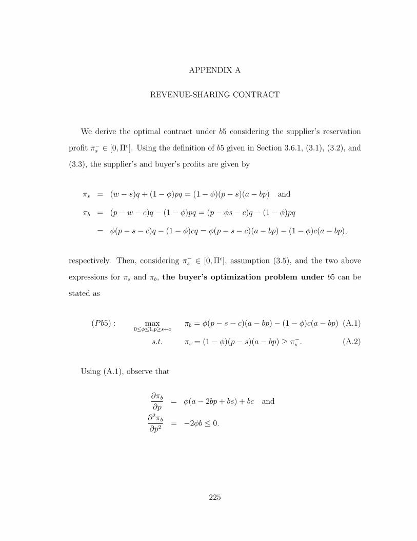
APPENDIX A
REVENUE-SHARING CONTRACT
We derive the optimal contract under b5 considering the supplier’s reservation
profit π−s ∈ [0,Πc]. Using the definition of b5 given in Section 3.6.1, (3.1), (3.2), and
(3.3), the supplier’s and buyer’s profits are given by
πs = (w − s)q + (1− ϕ)pq = (1− ϕ)(p− s)(a− bp) and
πb = (p− w − c)q − (1− ϕ)pq = (p− ϕs− c)q − (1− ϕ)pq
= ϕ(p− s− c)q − (1− ϕ)cq = ϕ(p− s− c)(a− bp)− (1− ϕ)c(a− bp),
respectively. Then, considering π−s ∈ [0,Πc], assumption (3.5), and the two above
expressions for πs and πb, the buyer’s optimization problem under b5 can be
stated as
(Pb5) : max0≤ϕ≤1,p≥s+c
πb = ϕ(p− s− c)(a− bp)− (1− ϕ)c(a− bp) (A.1)
s.t. πs = (1− ϕ)(p− s)(a− bp) ≥ π−s . (A.2)
Using (A.1), observe that
∂πb
∂p= ϕ(a− 2bp+ bs) + bc and
∂2πb
∂p2= −2ϕb ≤ 0.
225

Hence, πb is concave in p. Setting ∂πb/∂p = 0 leads to
pb5(ϕ) =a+ b(s+ c)
2b+
(1− ϕ)bc
2bϕ. (A.3)
Also, using (A.1), observe that
∂πb
∂ϕ= (p− s)(a− bp) > 0.
Hence, πb is increasing in ϕ, ϕ ∈ [0, 1]. Therefore, πb achieves the maximum at the
boundary of ϕ = 1 or πs = π−s .
• When ϕ = 1, by (A.2), πs = 0 and (A.2) are satisfied only if π−s = 0. In this
case, the supplier does not make any profit. The case is not practical and can
be discarded.
• If π−s > 0 then πs = π−
s and ϕ < 1. Using (A.3) in (A.2), we have
πs = (1− ϕ)b
[(a− bs
2b
)2
−(
c
2ϕ
)2]= π−
s . (A.4)
Next, we consider c = 0 and c > 0, separately.
– If c = 0 then using (A.4),
πs = (1− ϕ)(a− bs)2
4b= π−
s ⇒ ϕb5 = 1− π−s
Πc,
where Πc = (a− bs)2/4b given in (3.11). Also, (A.3) implies
pb5 =a+ bs
2b= pc.
226

Since ϕb5 and pb5 are realizable over the regions in (A.1), they characterize
the optimal b5. Then, using the definition of b5, (A.1) and (A.2), we have
Lb5 =(a+ bs)(a− bs)π−
s
4bΠc,
wb5 =
(1− π−
s
Πc
)s,
πb5s = π−
s ,
πb5b = Πc − π−
s , and
Πb5 = Πc,
where superscript for b5 is used in an obvious fashion. Clearly, the optimal
b5 is the coordination contract if c = 0.
– If c > 0 then using (A.3), pb5(ϕ) > pc = a+b(s+c)2b
is true for all ϕ ∈ [0, 1).
Hence, the contract is not a coordination contract if c > 0.
227