contrail study with ground-based cameras

AMTD6, 7425–7472, 2013

Contrail cameraobservations

U. Schumann et al.

Title Page

Abstract Introduction

Conclusions References

Tables Figures

J I

J I

Back Close

Full Screen / Esc

Printer-friendly Version

Interactive Discussion

Discussion

Paper

|D

iscussionP

aper|

Discussion

Paper

|D

iscussionP

aper|

Atmos. Meas. Tech. Discuss., 6, 7425–7472, 2013www.atmos-meas-tech-discuss.net/6/7425/2013/doi:10.5194/amtd-6-7425-2013© Author(s) 2013. CC Attribution 3.0 License.

EGU Journal Logos (RGB)

Advances in Geosciences

Open A

ccess

Natural Hazards and Earth System

Sciences

Open A

ccess

Annales Geophysicae

Open A

ccess

Nonlinear Processes in Geophysics

Open A

ccess

Atmospheric Chemistry

and Physics

Open A

ccess

Atmospheric Chemistry

and Physics

Open A

ccess

Discussions

Atmospheric Measurement

Techniques

Open A

ccess

Atmospheric Measurement

Techniques

Open A

ccess

Discussions

Biogeosciences

Open A

ccess

Open A

ccess

BiogeosciencesDiscussions

Climate of the Past

Open A

ccess

Open A

ccess

Climate of the Past

Discussions

Earth System Dynamics

Open A

ccess

Open A

ccess

Earth System Dynamics

Discussions

GeoscientificInstrumentation

Methods andData Systems

Open A

ccess

GeoscientificInstrumentation

Methods andData Systems

Open A

ccess

Discussions

GeoscientificModel Development

Open A

ccess

Open A

ccess

GeoscientificModel Development

Discussions

Hydrology and Earth System

SciencesO

pen Access

Hydrology and Earth System

Sciences

Open A

ccess

Discussions

Ocean Science

Open A

ccess

Open A

ccess

Ocean ScienceDiscussions

Solid Earth

Open A

ccess

Open A

ccess

Solid EarthDiscussions

The Cryosphere

Open A

ccess

Open A

ccess

The CryosphereDiscussions

Natural Hazards and Earth System

Sciences

Open A

ccess

Discussions

This discussion paper is/has been under review for the journal Atmospheric MeasurementTechniques (AMT). Please refer to the corresponding final paper in AMT if available.

Contrail study with ground-basedcamerasU. Schumann1, R. Hempel2, H. Flentje3, M. Garhammer4, K. Graf1, S. Kox1,H. Lösslein4, and B. Mayer4

1Deutsches Zentrum für Luft- und Raumfahrt, Institut für Physik der Atmosphäre,Oberpfaffenhofen, Germany2Deutsches Zentrum für Luft- und Raumfahrt, Simulations- und Softwaretechnik,Cologne, Germany3Deutscher Wetterdienst, Meteorologisches Observatorium Hohenpeissenberg,Hohenpeissenberg, Germany4Meteorologisches Institut, Ludwig-Maximilians-Universität, Munich, Germany

Received: 7 August 2013 – Accepted: 8 August 2013 – Published: 19 August 2013

Correspondence to: U. Schumann ([email protected])

Published by Copernicus Publications on behalf of the European Geosciences Union.

7425

http://www.atmos-meas-tech-discuss.net

http://www.atmos-meas-tech-discuss.net/6/7425/2013/amtd-6-7425-2013-print.pdf

http://www.atmos-meas-tech-discuss.net/6/7425/2013/amtd-6-7425-2013-discussion.html

http://creativecommons.org/licenses/by/3.0/

AMTD6, 7425–7472, 2013


U. Schumann et al.

Title Page



Tables Figures

J I

J I

Back Close

Full Screen / Esc



Discussion

Paper

|D

iscussionP

aper|

Discussion

Paper

|D

iscussionP

aper|

Abstract

Photogrammetric methods and analysis results for contrails observed with wide-anglecameras are described. Four cameras of two different types (view angle<90◦ or whole-sky imager) at the ground at various positions are used to track contrails and to derivetheir altitude, width, and horizontal speed. Camera models for both types are described5

to derive the observation angles for given image coordinates and their inverse. Themodels are calibrated with sightings of the Sun, the Moon and a few bright stars. Themethods are applied and tested in a case study. Four persistent contrails crossingeach other together with a short-lived one are observed with the cameras. Verticaland horizontal positions of the contrails are determined from the camera images to an10

accuracy of better than 200 m and horizontal speed to 0.2 m s−1. With this information,the aircraft causing the contrails are identified by comparison to traffic waypoint data.The observations are compared with synthetic camera pictures of contrails simulatedwith the contrail prediction model CoCiP, a Lagrangian model using air traffic movementdata and numerical weather prediction (NWP) data as input. The results provide tests15

for the NWP and contrail models. The cameras show spreading and thickening contrailssuggesting ice-supersaturation in the ambient air. The ice-supersaturated layer is foundthicker and more humid in this case than predicted by the NWP model used. Thesimulated and observed contrail positions agree up to differences caused by uncertainwind data. The contrail widths, which depend on wake vortex spreading, ambient shear20

and turbulence, were partly wider than simulated.

1 Introduction

Contrails are linear clouds often visible to ground observers behind cruising air-craft. The conditions under which contrails form (at temperatures below the Schmidt–Appleman criterion) and persist (at ambient humidity exceeding ice saturation) are25

well known (Schumann, 1996). The dynamics of young contrails depend on aircraft

7426





AMTD6, 7425–7472, 2013


U. Schumann et al.

Title Page



Tables Figures

J I

J I

Back Close

Full Screen / Esc



Discussion

Paper

|D

iscussionP

aper|

Discussion

Paper

|D

iscussionP

aper|

emissions and wake properties and the pattern of contrails changes over their lifetime(Lewellen and Lewellen, 1996; Sassen, 1997; Mannstein et al., 1999; Jeßberger et al.,2013). Though contrails have been investigated for some time, still little is known aboutthe full life cycle of individual contrails (Mannstein and Schumann, 2005; Heymsfieldet al., 2010; Unterstrasser and Sölch, 2010; Graf et al., 2012; Minnis et al., 2013; Schu-5

mann and Graf, 2013).Ground-based contrail observations may help to understand contrail dynamics and

ice formation (Freudenthaler et al., 1995; Immler et al., 2008). The observable contrailcover can be predicted with contrail simulation models (Stuefer et al., 2005; Duda et al.,2009; Schumann, 2012). Such models require numerical weather prediction (NWP)10

data and traffic data as input and observations for validation. Here, we use NWP dataas available from the Integrated Forecast System (IFS) model of the European Cen-tre for Medium Range Forecasts (ECMWF). Information on air traffic can, since a fewyears, be received online from so-called flight radar data in the internet, including air-craft positions transmitted by Automatic Dependent Surveillance-Broadcast (ADSB), at15

least from the majority of aircraft which have such equipment (Jackson et al., 2005; deLeege et al., 2012).

Wide-angle digital cameras have been used before to observe clouds (e.g. Seizet al., 2007) and contrails (Sassen, 1997; Feister and Shields, 2005; Stuefer et al.,2005; Atlas and Wang, 2010; Feister et al., 2010; Mannstein et al., 2010; Shields et al.,20

2013). Whole-sky imagers using fisheye lens image the full sky down or nearly downto the horizon (Shields et al., 2013). More narrow wide-angle cameras cover only partof the sky but with higher resolution. Besides color cameras also multispectral cam-eras recording in several spectral wavebands are available (Feister and Shields, 2005;Seiz et al., 2007; Shields et al., 2013). Camera observations often reveal interesting25

cloud properties, but a single camera is insufficient to determine the distance of anobservable object (LeMone et al., 2013). A video scene from a single camera allowsdetermining the angular but not the linear cloud speed. Horizontal contrail positionscan be estimated if the contrail altitude is known from other sources (Atlas and Wang,

7427





AMTD6, 7425–7472, 2013


U. Schumann et al.

Title Page



Tables Figures

J I

J I

Back Close

Full Screen / Esc



Discussion

Paper

|D

iscussionP

aper|

Discussion

Paper

|D

iscussionP

aper|

2010). A network of cameras has been used for observations of upper atmosphereclouds (Baumgarten et al., 2009) and other objects (Shields et al., 2013).

In regions with dense air traffic, the sky is often full of contrails, and the assignment ofindividual observed contrails to specific aircraft requires accurate contrail altitudes be-sides traffic information. The analysis of aged contrails requires the trajectory analysis5

from aircraft flight routes to contrail positions.Here, we report on a case study where we observed contrails with four wide-angle

cameras, placed several km apart and oriented at fixed positions in the sky, provid-ing digital images every 10 s. If the same cloud detail could be identified in overlap-ping areas of stereo images taken with at least two cameras simultaneously, its three-10

dimensional position could be determined (Seiz et al., 2007). In our case, the horizontaldistance between the cameras was too large for simultaneous observations, but cloudfeatures moving with about constant speed across the camera view-fields could beused for photogrammetric analysis. The results are used to identify the causing air-craft, contrail positions vs. time with respect to NWP data, and to deduce contrail and15

atmospheric properties. For a direct comparison of simulated contrails with camera ob-servations, we map the computed contrails on synthetic camera images. This requiresalgorithms which compute spherical coordinates for given pixel coordinates and theirinverse.

The pixel positions of identifiable objects in digital camera images can be determined20

with standard image processing software. However, images of wide-angle camerasusually are distorted considerably (Weng et al., 1992; Garcia et al., 1997). In our casethe distortion becomes obvious because straight contrails appear increasingly curvedwhen coming close to the camera position, in particular near the edge of the cameraimage. The mathematical algorithm which describes the transformation of image co-25

ordinates into horizontal spherical coordinates or vice versa, including corrections fordistortion is called a camera model.

Camera models have been used widely for astronomical observations, mainly fordark sky imaging, e.g. for meteor trace analysis (Oberst et al., 2004), also for gravity

7428





AMTD6, 7425–7472, 2013


U. Schumann et al.

Title Page



Tables Figures

J I

J I

Back Close

Full Screen / Esc



Discussion

Paper

|D

iscussionP

aper|

Discussion

Paper

|D

iscussionP

aper|

wave analysis in mesospheric airglow images (Garcia et al., 1997), noctilucent cloudobservations (Baumgarten et al., 2009), cloud mapping using calibration with stars andaircraft with known positions (Seiz et al., 2007; Shields et al., 2013), or for automaticidentification of stars in digital images (Klaus et al., 2004).

In contrast to stars, cloud features are more fuzzy and variable in time, and hence5

only allow less accurate geometric observations. Contrail features cover typically ob-servation angles of one or a few degrees. Therefore, our camera model uses a sim-plified imaging geometry and distortion model and exploits symmetry assumptions tocover the full image frame.

This article describes camera models for two types of wide-angle cameras (a whole-10

sky imager and a more narrow one). The camera models correct for radial distortioninside the camera and for the orientation of the camera with respect to the horizontalcoordinate system. The camera models are calibrated by using observations of theSun, the Moon, planets and a few bright stars and landmarks. Moreover, we reportresults from aircraft track and contrail motion analysis with the camera models, and15

compare them with air traffic movement data, numerical weather prediction data, andsimulations of contrail trajectories and spreading with a Lagrangian contrail model.

2 Camera models

2.1 The cameras used

Cloud images were obtained in this study with four commercial digital video color cam-20

eras (Table 1). Photogrammetric analysis is described in detail for two of them (Fig. 1):

1. A wide-angle camera of type Mobotix D24M with L22 lens, installed on the roofof the Institute of Atmospheric Physics of the Deutsches Zentrum für Luft- undRaumfahrt (DLR, German Aerospace Center) at Oberpfaffenhofen (OP). Thewide-angle lens covers a limited field of view and faces roughly westward with25

some upward tilting.7429





AMTD6, 7425–7472, 2013


U. Schumann et al.

Title Page



Tables Figures

J I

J I

Back Close

Full Screen / Esc



Discussion

Paper

|D

iscussionP

aper|

Discussion

Paper

|D

iscussionP

aper|

2. A whole-sky fisheye camera of type Mobotix Q24M installed on the roof of theMeteorological Institute of the Ludwig-Maximilians-Universität in Munich (MIM),pointing vertically.

The local time of observation, received from an internet time server, is recorded withan accuracy of about 1 s. The two further cameras, MAY and HOP, are also of type 1,5

as the OP camera.

2.2 Camera model algorithms

The camera model provides the relationship between celestial azimuth and elevationangle coordinates (A, E) and pixel coordinates (X , Y ). X counts image columns fromleft to right, from 1 to 2048 and 1 to 1280, for camera 1 and 2, respectively; Y counts10

image rows from top to bottom, 1 to 1536 and 1 to 960. The azimuth A varies from0 to 360◦ (0◦: North, 90◦: East). The elevation is zero at the horizon and 90◦ at thezenith. The algorithm makes use of the pixel and celestial coordinates of the cameramid-points, (X0, Y0, A0, E0). For camera 1, the coordinates X0 and Y0 are set to themidpoint of the image plane and the angles A0 and E0 are found from astronomical15

observations near this midpoint. For camera 2, the midpoint is set to coincide with thevertical direction (E = 90◦, A = 0◦) and the values of the coordinates X0 and Y0 arefound by minimizing the model residuals, i.e. the root-mean square (rms) differencesbetween observed and computed star observations. A large focal length of the camerasis important for high resolution (Table 1), but its value is not used explicitely in the20

models.The camera model describes the mapping between pixel coordinates (X , Y ) in the

image and (X ′,Y ′) coordinates in an imaginary plane onto which the spherical objectcoordinates (A, E) are projected (the so-called projection plane). The two camera typesdiffer in their mapping transformations (see Fig. 3). For camera 1, which is the upward25

tilted, the projection plane is the plane tangential to the celestial unit sphere, with thetangential point being at the image center. The rectangular coordinates in this plane are

7430





AMTD6, 7425–7472, 2013


U. Schumann et al.

Title Page



Tables Figures

J I

J I

Back Close

Full Screen / Esc



Discussion

Paper

|D

iscussionP

aper|

Discussion

Paper

|D

iscussionP

aper|

defined by gnomonic projection. For camera 2, the lens projects the sky onto a horizon-tal finite circular image resolved by a rectangular set of image pixels. Here, we choosethe horizontal plane as projection plane, with the position angle of an object’s projectionpoint being its azimuth, and the center distance being proportional to its zenith distanceangle. An affine transformation is constructed between the two Cartesian coordinate5

systems.Additionally, the camera model accounts for the distortion caused by the camera

lens, i.e. its deviation from the ideal geometry of a so-called pinhole camera (van deKamp, 1967). We assume that radial lens distortions are symmetric with respect torotation around the image center. Instead of a polynomial function (e.g. Weng et al.,10

1992), we use an exponential function because of well-defined asymptotic behavior forsmall and large radius arguments.

With these definitions, we compute the parameters of the camera models as follows.First, we determine the parameters of the distortion function by comparing for all obser-vations their center distances in the image with those in the projection plane. We then15

use the distortion function to rectify the observed pixel coordinates. Finally, followingthe classical Turner method (Turner, 1894), we construct an affine transformation be-tween the rectified pixel coordinates and the computed locations of the celestial objectsin the projection plane. This transformation represents the camera orientation and im-age scaling. Since the problem is over-determined, least-square fits are applied in the20

parameter computations for both the distortion function and the affine transformation.Based on these considerations, the forward transformation

(A,E) = f (X ,Y ) (1)

is constructed as follows:

1. The camera pixels (X , Y ) are transformed into rectangular coordinates (xd , yd )25

relative to the camera center, with yd pointing upwards in the image,

xd = X −X0, yd = Y0 −Y . (2)7431





AMTD6, 7425–7472, 2013


U. Schumann et al.

Title Page



Tables Figures

J I

J I

Back Close

Full Screen / Esc



Discussion

Paper

|D

iscussionP

aper|

Discussion

Paper

|D

iscussionP

aper|

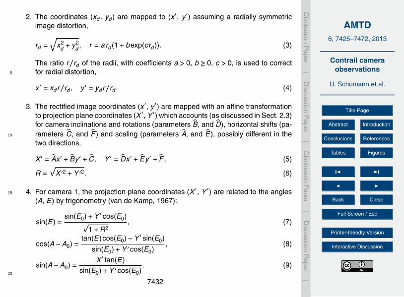
2. The coordinates (xd , yd ) are mapped to (x ′, y ′) assuming a radially symmetricimage distortion,

rd =√

x2d + y2

d , r = ard (1+b exp(crd )). (3)

The ratio r/rd of the radii, with coefficients a > 0, b ≥ 0, c > 0, is used to correctfor radial distortion,5

x ′ = xd r/rd , y ′ = yd r/rd . (4)

3. The rectified image coordinates (x ′, y ′) are mapped with an affine transformationto projection plane coordinates (X ′, Y ′) which accounts (as discussed in Sect. 2.3)for camera inclinations and rotations (parameters B, and D), horizontal shifts (pa-rameters C, and F ) and scaling (parameters A, and E), possibly different in the10

two directions,

X ′ = Ax ′ + By ′ + C, Y ′ = Dx ′ + Ey ′ + F , (5)

R =√

X ′2 +Y ′2. (6)

4. For camera 1, the projection plane coordinates (X ′, Y ′) are related to the angles15

(A, E) by trigonometry (van de Kamp, 1967):

sin(E) =sin(E0)+Y ′ cos(E0)

√1+R2

, (7)

cos(A−A0) =tan(E)cos(E0)−Y ′ sin(E0)

sin(E0)+Y ′ cos(E0), (8)

sin(A−A0) =X ′ tan(E)

sin(E0)+Y ′ cos(E0). (9)

20

7432





AMTD6, 7425–7472, 2013


U. Schumann et al.

Title Page



Tables Figures

J I

J I

Back Close

Full Screen / Esc



Discussion

Paper

|D

iscussionP

aper|

Discussion

Paper

|D

iscussionP

aper|

For camera 2, we use:

E = 90◦(1−R), cos(A) = Y ′/R, sin(A) = X ′/R. (10)

5. Finally, equations sin(A′) = SA, cos(A′) = CA, with given SA, CA, imply if CA > 0:A′ = sin−1(SA), else: A′ = 180◦ − sin−1(SA). Negative values of A are incrementedby 360◦.5

The inverse transformation

(X ,Y ) = F (A,E) (11)

is set-up consistently as follows.

1. Camera 1 uses the gnomonic projection of the angles (A,E) to camera imagecoordinates (X ′,Y ′) (van de Kamp, 1967):10

X ′ =cos(E)sin(A−A0)

sin(E)sin(E0)+ cos(E)cos(E0)cos(A−A0), (12)

Y ′ =sin(E)cos(E0)− cos(E)sin(E0)cos(A−A0)

sin(E)sin(E0)+ cos(E)cos(E0)cos(A−A0), (13)

R =√

X ′2 +Y ′2. (14)

Camera 2 uses the inverse of Eq. (10),15

R = (90◦ −E)/90◦, X ′ = R sin(A), Y ′ = R cos(A). (15)

For both cameras, we compute the inverse of Eq. (5):

y ′ =D(X ′ − C)+ A(F −Y ′)

BD − EA, (16)

x ′ = (X ′ − By ′ − C)/A, r =√

x ′2 + y ′2. (17)20

7433





AMTD6, 7425–7472, 2013


U. Schumann et al.

Title Page



Tables Figures

J I

J I

Back Close

Full Screen / Esc



Discussion

Paper

|D

iscussionP

aper|

Discussion

Paper

|D

iscussionP

aper|

The inverse solution rd (r ) of Eq. (3) is determined by a Newton iteration, startingfrom a first guess rd = r/a. Finally the pixel coordinates are given by

xd = x ′rd/r , yd = y ′rd/r , X = xd +X0, Y = Y0 − yd . (18)

In total, both cameras use 11 free model parameters: A, B, C, D, E , F , a,b,c,E0,A0for camera 1, and X0,Y0 instead of E0,A0 for camera 2. To avoid a conflict in scaling5

by a and the Turner coefficients, we normalize the latter such that the determinanteAE−BD = 1. This reduces the number of free parameters to 10. For their calibration, weassume that a set of observations (Ai ,Ei ,Xi ,Yi ), i = 1,2, . . .,n, is available (see Fig. 3).In the following we will show how these parameters are determined.

For each observation, we compute R(Ai ,Ei ) from Eqs. (2–6) and R(Xi ,Yi ) from10

Eqs. (12–15). Ideally, both should be equal. Here, we determine the fitting parame-ters a,b,c entering Eq. (3) such that the differences have minimum rms values,

SR =n∑i

(R(Ai ,Ei )−R(Xi ,Yi ))2. (19)

Using Eqs. (3) and (4), we compute ri , x ′i , y ′

i for each observation. Together with theX ′

i , Y ′i from above, these data should satisfy Eq. (5):15

X ′i = Ax ′

i + By ′i + C, Y ′

i = Dx ′i + Ey ′

i + F , i = 1,2, . . .,n, (20)

with unknowns A, B, C, D, E , F . This set of equations can be expressed in matrix nota-tion as

(X ′

i

)= Jx

ABC

,(Y ′

i

)= Jy

DEF

. (21)

7434





AMTD6, 7425–7472, 2013


U. Schumann et al.

Title Page



Tables Figures

J I

J I

Back Close

Full Screen / Esc



Discussion

Paper

|D

iscussionP

aper|

Discussion

Paper

|D

iscussionP

aper|

For n > 3, Eqs. (21) are over-determined. A least-square solution for the model pa-rameters is found by solving the normal equations,

JTx Jx

ABC

= JTx(X ′

i

), JT

y Jy

DEF

= JTy(Y ′

i

). (22)

These linear systems with 3 unknowns each are solved numerically.Optimal values of A0,E0 (camera 1) or X0,Y0 (camera 2) are found when minimizing5

the properly weighted sums of the squared residuals of the observations for anglesand pixel coordinates together with the radial residuals (Eq. 19). The camera modelsare available as implementations in MS Excel 2010, Python, and Fortran, using variousoptimisation algorithms (e.g. Schumann et al., 2012).

2.3 Camera calibration observations10

For the determination of the camera model parameters (Table 2), we need a set of coor-dinates (Xi ,Yi ), i = 1,2, . . .,n, related to known azimuth and elevation (Ai ,Ei ). Basically,n = 3 linearly independent pairs of (precise) observations are sufficient to determinethe 6 coefficients of the affine transformations (Eq. 5). At least 3 (partly the same) ob-servations spaced over the radial range are needed to determine the 3 coefficients in15

the radial distortion function (Eq. 3). However, to compensate for observation errors,a large set of observations covering the whole field of view is desirable, n � 3.

Here, we describe calibration for cameras OP and MIM. For these cameras, we useoccasional sightings of celestial objects in images taken at times with clear sky. Sincethe orientation of the cameras is fixed, sightings taken at different, accurately measured20

times can be used for a single camera model.In the actual application, the field coverage is far from optimal. One of the cameras

was operated routinely only during day time. Moreover, because of strong stray light atthe urban observation positions, only a few usable night time observations are avail-

7435





AMTD6, 7425–7472, 2013


U. Schumann et al.

Title Page



Tables Figures

J I

J I

Back Close

Full Screen / Esc



Discussion

Paper

|D

iscussionP

aper|

Discussion

Paper

|D

iscussionP

aper|

able. Therefore, the cameras are calibrated using observations of the Sun, Moon, andVega for OP, and the Sun, Moon, Venus, Jupiter, and Sirius for MIM.

For these sightings, the coordinates of the brightest pixel are measured at high mag-nification using the software Irfanview. The planetarium software Guide 9.0 provideshigh-precision spherical coordinates with respect to the horizon, including the correc-5

tion for atmospheric refraction, for the times when the digital images were taken.For OP, the sightings are concentrated in essentially two image bands (see Fig. 3).

One band (mainly Sun, some Moon and some Vega observations) runs from the upper-left to the lower-right corner and crosses the middle of the image. The other one (Moonobservations) is parallel to the first and lies closer to the lower-left corner. Measure-10

ments in the upper-right or lower-left image corner are missing. Observations of land-marks at low elevation angles at distances between 130 and 360 m are used for inde-pendent model tests (see Fig. 4).

For MIM, observations are available mainly in the South. The northern range of az-imuth angles between 292◦ and 72◦ is not covered. Three landmarks at low elevation15

angles at distances between 200 and 4500 m are used again for tests (see Fig. 4).As a result, with coefficients as given in Table 2, the image resolution in degree per

pixel, as derived from derivatives such as ∂A/∂X , is 0.052 in A and 0.045 in E at theimage mid-point in OP, and 0.158 in E at the zenith and 0.109 and 0.215 in A and E atthe horizon of the MIM camera. The resolution for MIM is slightly better than what was20

reported for multispectral whole-sky cameras before (Feister and Shields, 2005; Seizet al., 2007).

The resolution is sufficient to observe contrails at ` = 100 m geometric scales up toa range radius R` = `NX 180◦/(π∆A) of more than 22 km (see Table 1). Here, NX isthe number of image pixels in horizontal direction and ∆A is the azimuth angle range.25

For cameras OP, MAY, and HOP, this range is computed for elevation E0. For MIM, wecompute the range at zero elevation with NX/∆A = ∂X/∂A.

7436





AMTD6, 7425–7472, 2013


U. Schumann et al.

Title Page



Tables Figures

J I

J I

Back Close

Full Screen / Esc



Discussion

Paper

|D

iscussionP

aper|

Discussion

Paper

|D

iscussionP

aper|

2.4 Discussion of the model accuracy

The model accuracy is limited by two factors:

1. The model is no perfect description of the camera. For example, the image distor-tion function approximates an a priori unknown relation between measured andreal image center distances. A tangential distortion (Weng et al., 1992), e.g. is not5

taken into account.

2. The astronomical sightings are affected by measuring errors in the images. Theglare (or blooming effect, Seiz et al., 2007) caused by bright objects (Sun andMoon) and by the lens may cause errors of the order of several pixels, in particularclose to the image borders. Uncertainties in the celestial coordinates provided by10

the planetarium software are several orders of magnitude smaller and can beneglected.

The model accuracy is assessed by testing how well the model matches the as-tronomical sightings it is based on. Since there are many more sightings than modelparameters, residuals will be small only if the model is a good description of the real15

camera setup. The residuals of the camera model are computed from differences be-tween given and computed image coordinates. Both the maximum and the rms residu-als are evaluated (see Table 3). Further independent tests will be provided by sightingsof aircraft with known positions (see Sect. 3.3).

The rms angle residuals are in the range of 0.2◦ or smaller, and the pixel residuals20

in the range of 3 (see Table 3 and Fig. 4). The pixel residuals for MIM are smallerand the angular residuals are larger than for OP because of coarser angular resolutionper pixel. Given the short focal length of the cameras, and considering the fact thatthe angular diameter of the Sun and Moon is about 0.5◦, these residuals are withinthe expected measurement errors. Note, an angle error of 0.2◦ corresponds to 35 m25

displacement at 10 km altitude in the zenith above the MIM camera. The pixel residualsare larger, mainly because of glare, but comparable to the accuracy of cloud feature

7437





AMTD6, 7425–7472, 2013


U. Schumann et al.

Title Page



Tables Figures

J I

J I

Back Close

Full Screen / Esc



Discussion

Paper

|D

iscussionP

aper|

Discussion

Paper

|D

iscussionP

aper|

observations. The landmarks are at very low elevation angles and at small distances,which could be a source of additional uncertainty, but the residuals are in the samerange as for the other observations. Landmarks are time-independent and they showno systematic ∆A residuals, which would arise from astronomical observations if theimage time readings would be systematically high or low.5

To show the sensitivity to the distortion corrections (Eq. 3), we applied the model alsowithout the corrections. In this case, the rms residuals become about 20 times larger.The radial corrections mainly reduce elevation residuals, while the affine transformationmainly impacts azimuth values. The importance of the radial transformation can alsobe seen from the factor b (Table 2) which amounts to about 3.5 %. The exponential10

term becomes large for pixel radii larger than 1/c, of about 200 to 500.While small residuals are a good indicator for the model accuracy within the image

areas covered by observations, they cannot be used to assess the model quality inplaces where no observations are available. In those places the models are extrapo-lations based on symmetry assumptions. An important assumption is that the camera15

lenses exhibit a circular symmetry. For the radial distortion function an exponentialfunction was chosen which is free of artificial oscillations. This would be different, e.g. ifa polynomial would have been used. Tests have shown that the difference of predictionand measurement (in pixels) for the image distortion function, Eq. (3), does not exceedthe typical measuring errors of a few pixels independent of the position angles in the20

image.Finally, the observational data have to be sufficient for a stable computation of the

affine transformation (Eq. 5). The parameters in this transformation become ill-definedif the image area covered by observations degrades to a line. Fortunately, for bothcameras the covered areas have large extensions in both coordinate directions. For25

modern cameras, we may expect nearly non-skewed and isotropic pixel orientations,so that D ≈ −B, E ≈ A. Here, A and E differ by less than 0.01 % for both cameras.Small values of B and D are expected if the camera mounting is precisely aligned

7438





AMTD6, 7425–7472, 2013


U. Schumann et al.

Title Page



Tables Figures

J I

J I

Back Close

Full Screen / Esc



Discussion

Paper

|D

iscussionP

aper|

Discussion

Paper

|D

iscussionP

aper|

horizontally. These relationships can also be used to assess the quality of a limited setof observations.

2.5 Transformations between observation angles and geographic coordinates

For relating geographic positions of an object to camera observation angles, weuse Cartesian coordinates (x ,y ,z), in m, with the horizontal plane x–y tangential to5

a sphere, approximating the Earth with mean radius R ≈ 6371 km, at longitude λ = λC,latitude φ =φC, and altitude z = zC of the camera C above mean sea level (a.s.l.).Here, x ,y are the orthogonal horizontal geographic coordinates in eastern and north-ern directions and z is the vertical coordinate a.s.l. For small distances λ− λC andφ−φC, the coordinates x ,y are related to λ and φ, in degrees, approximately by10

x − xC = (λ− λC)R cos(φ)π/180◦, (23)

y − yC = (φ−φC)Rπ/180◦. (24)

For large λ− λC and φ−φC, great circle computations (van de Kamp, 1967; Earle,2005) are required instead.15

In the computation of the elevation angle E and the projected distance d on theground between the object and the camera we account for the curvature of the Earthsurface. Tests have shown that the curvature may be ignored for contrail altitude andwind speed determinations for altitudes above 8 km and distances below 50 km. Forlarger distances and low elevation angles, however, the curvature must be considered.20

An object at altitude H sinks below the horizon (E = 0) at the horizontal distance a =√2RH +H2; e.g. a = 35.7, 112.9, 357.1 km for H = 0.1, 1, 10 km, respectively.For an object P at altitude H + zc a.s.l. viewed from camera C at angles A,E above

Earth horizon with Earth origin in O and effective Earth radius R′ = R+zC (see Fig. 5),the general triangle OCP is defined by two given side lengths OC and OP and one25

angle, ψ = d/R or α = E +90◦. Hence, we find the distance d along the Earth surfaceat sea level and the geographic coordinates (x ,y ) = g(A,E ,H) from

7439





AMTD6, 7425–7472, 2013


U. Schumann et al.

Title Page



Tables Figures

J I

J I

Back Close

Full Screen / Esc



Discussion

Paper

|D

iscussionP

aper|

Discussion

Paper

|D

iscussionP

aper|

α = E +π/2, sin(β) =R′ sin(α)

R′ +H, ψ = π−β−α, (25)

d = ψR, x = xC +d sin(A), y = yC +d cos(A). (26)

Inversely, for given position (x ,y ) of an object P with altitude H+zc a.s.l., the distanced and the angles (A,E) = G(x ,y ,H) of visual appearance of P from C are determined5

by

d =√

(x − xC)2 + (y − yC)2, (27)

ψ =dR

, tan(γ) =H

2R′ +H1

tan(ψ/2), (28)

E = γ −ψ/2, A = tan−1[(x − xC)/(y − yC)]. (29)10

Similar relationships to compute A,E for given x ,y ,H are given in Garcia et al.(1997), but ours are simpler and allow for explicit inversion to compute x ,y for givenA,E ,H.

3 A four-contrail-cross case study

3.1 Observations15

We observed four crossing contrails passing the view field of camera OP at about08:42 UTC 3 November 2012 (see Fig. 6) (all the clock times refer to UTC). The airwas clear with at least 100 km visibility. Wind was strong from about west with about50 m s−1 (e.g. according to ECMWF data) at the contrails’ altitudes, so that the con-trails happened to move into the direction of Munich. Because of the cross pattern, the20

same set of contrails was clearly identified at MIM about 10 min later. The contrails are7440





AMTD6, 7425–7472, 2013


U. Schumann et al.

Title Page



Tables Figures

J I

J I

Back Close

Full Screen / Esc



Discussion

Paper

|D

iscussionP

aper|

Discussion

Paper

|D

iscussionP

aper|

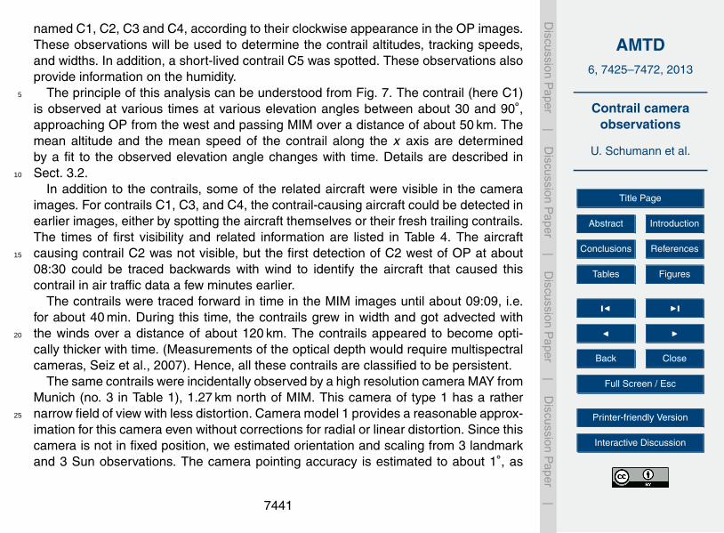
named C1, C2, C3 and C4, according to their clockwise appearance in the OP images.These observations will be used to determine the contrail altitudes, tracking speeds,and widths. In addition, a short-lived contrail C5 was spotted. These observations alsoprovide information on the humidity.

The principle of this analysis can be understood from Fig. 7. The contrail (here C1)5

is observed at various times at various elevation angles between about 30 and 90◦,approaching OP from the west and passing MIM over a distance of about 50 km. Themean altitude and the mean speed of the contrail along the x axis are determinedby a fit to the observed elevation angle changes with time. Details are described inSect. 3.2.10

In addition to the contrails, some of the related aircraft were visible in the cameraimages. For contrails C1, C3, and C4, the contrail-causing aircraft could be detected inearlier images, either by spotting the aircraft themselves or their fresh trailing contrails.The times of first visibility and related information are listed in Table 4. The aircraftcausing contrail C2 was not visible, but the first detection of C2 west of OP at about15

08:30 could be traced backwards with wind to identify the aircraft that caused thiscontrail in air traffic data a few minutes earlier.

The contrails were traced forward in time in the MIM images until about 09:09, i.e.for about 40 min. During this time, the contrails grew in width and got advected withthe winds over a distance of about 120 km. The contrails appeared to become opti-20

cally thicker with time. (Measurements of the optical depth would require multispectralcameras, Seiz et al., 2007). Hence, all these contrails are classified to be persistent.

The same contrails were incidentally observed by a high resolution camera MAY fromMunich (no. 3 in Table 1), 1.27 km north of MIM. This camera of type 1 has a rathernarrow field of view with less distortion. Camera model 1 provides a reasonable approx-25

imation for this camera even without corrections for radial or linear distortion. Since thiscamera is not in fixed position, we estimated orientation and scaling from 3 landmarkand 3 Sun observations. The camera pointing accuracy is estimated to about 1◦, as

7441





AMTD6, 7425–7472, 2013


U. Schumann et al.

Title Page



Tables Figures

J I

J I

Back Close

Full Screen / Esc



Discussion

Paper

|D

iscussionP

aper|

Discussion

Paper

|D

iscussionP

aper|

supported by the observation of an aircraft with a shortly visible contrail, the position ofwhich is given by ADSB data.

Finally a low resolution webcam HOP (no. 4 in Table 1) of the Observatory Ho-henpeissenberg (Deutscher Wetterdienst), 37.53 km southwest of OP, calibrated witha few Sun, Moon, star (Arcturus and Vega), and landmark observations, documents5

the scene in westward direction.

3.2 Contrail altitude and wind speed

Without knowing the aircraft waypoints, the contrail altitude z can be determined bya least-square fit assuming the observed contrail positions can be tracked along linesat constant altitude with constant wind speeds U,V in east/north (x ,y ) directions. For10

this purpose, we measure manually coordinate pairs (X ,Y ) for selected points withinthe contrail in images taken at various times and locations (here in 3 images from OPand 3 from MIM at times between 08:39 and 08:56 UTC). For wider contrails we usethe higher (in elevation for OP, or most eastward for MIM) contrail edge to capturethe contrail tops. From the pixel coordinates, the azimuth and elevation (A,E) pairs15

are computed using the camera model (Eq. 1). With estimated altitude z (e.g. 10 km),the distance d and the horizontal geographic coordinates (x ,y ) are computed fromEq. (26), and then the altitude is corrected iteratively to minimize the rms to the obser-vations, as described below. The final results are shown in Fig. 8.

The contrail coordinates (x ,y ) are assumed to be close to straight lines20

yc(t) = C(t)+ s(t)xc(t). (30)

The values C and s at various times are fitted so that the sum of (x−xc)2+(y−yc)2 overall points along a contrail in one image assumes its minimum. The plots in Fig. 8 showthat the contrails are in fact very close to linear. This also shows that the camera modelcorrectly removes the distortion of straight lines. For a moving line without marked25

features, one can determine the tracking speed only in the normal direction. Here, we

7442





AMTD6, 7425–7472, 2013


U. Schumann et al.

Title Page



Tables Figures

J I

J I

Back Close

Full Screen / Esc



Discussion

Paper

|D

iscussionP

aper|

Discussion

Paper

|D

iscussionP

aper|

follow the advection of the cross point at xc = −C/s between the contrail lines and aneast-west axis (yc = 0) through the camera point at OP. For given nonzero slope s,this point moves with constant advection speed Ua = U −V/s. Note that the computedgeographic coordinates X ,Y depend on altitude H = z − zC by Eq. (26). The altitudez a.s.l., the speed Ua, and the reference coordinate x0 are free parameters which5

are determined with an optimization routine such that xc(t) = x0 +Uat agrees with theobserved contrail line crossing point in the least square sense. This works for slopess significantly different from zero. In this case, we have 3 unknowns (z,x0,Ua) and 6measurements (xc at the 6 observation times), hence this minimization process hasa well-defined solution. For contrails nearly parallel to the wind direction (C4 in our10

example), we need to identify contrail features (here the end points) which can beassumed to move with constant wind speed (U,V ).

Table 4 lists the results. The fit results are accurate of up to 200 m rms errors forz, and 0.23 ms−1 for advection or wind speed. This was found out by systematicallyrepeating the analysis with random selections of subsets of the camera readings X ,Y .15

The contrail altitudes derived from the camera fits can be compared with the aircraftflight level information (see Table 4). Note that the camera observes the geometricaltitude. Aircraft flight levels (FL) are pressure altitudes in hft defined for static pressurein the International Civil Aviation Organization (ICAO) standard atmosphere (ICAO,1964). In our case, with lower than average surface pressure and warmer atmosphere20

up to 8 km, the geometric (or geopotential) altitude zg is ∆zICAO = 200±35 m higherthan the ICAO pressure altitude zp, according to ECMWF data, for this case. Hence,the effective altitude difference is zg − zp −∆zICAO. With this correction, these altitudedifferences are within ±163 m (see Table 4).

These differences differ slightly from the camera fit rms errors. Note that the lower25

part of a contrail sinks during the wake vortex phase by a range of the order of 50–300 m depending on aircraft and atmosphere parameters (e.g. Schumann et al., 2013).Differences may also result from uncertain pixel readings for thick contrails, horizontalvariations in the wind speed (the U wind component seems to increase with y ), and

7443





AMTD6, 7425–7472, 2013


U. Schumann et al.

Title Page



Tables Figures

J I

J I

Back Close

Full Screen / Esc



Discussion

Paper

|D

iscussionP

aper|

Discussion

Paper

|D

iscussionP

aper|

atmospheric wave motions. However, the accuracy of the derived contrail altitudes isconsistent with stereo camera cloud altitude results (Seiz et al., 2007).

The effective advection speed U−V/s agrees within about 2 % with the correspond-ing values derived from ECMWF data for 09:00 UTC this day, see Table 4. The windspeed components U and V derived for case C4 at 8.7 km altitude agree within 5 %5

with the ECMWF data (44.5 and 6 ms−1), see Fig. 13.For analysis of contrail widths, we use overlays of horizontal x–y grids into the image,

as shown for example in Fig. 9. The geographic grid coordinates x ,y ,z are specified forgiven contrail altitudes and given horizontal resolution. The view angles A,E and theimage coordinates X ,Y are computed using Eqs. (1) and (29). The widths observed10

over OP and MIM, as listed in Table 4, are determined by matching the observed con-trails with the grid, with about 100 m accuracy. The width of the short-lived contrail C5is at the limit of resolution. For the others, the width accuracy is limited mainly by thecontrail shape and contrail edge contrast against clear sky. With time, the persistentcontrails become wider. The width for C3 includes the sum of primary and secondary15

wake parts which can be visually distinguished in this case. Because of positive windshear, the primary wake appears at the more westward edge.

3.3 Aircraft identification

For contrails C1, C3, and C5, the pixel coordinates X ,Y of the aircraft sightings weremeasured (typically with ±2 pixel uncertainties). For C4, the first contrail appearance20

was located in the OP camera images. These data were converted into azimuth andelevation angles A,E using the OP camera model, Eq. (1). With this information and anestimated altitude z, we use Eq. (26) to estimate the geographic horizontal coordinates(x ,y ,z, t) of the first contrail sightings.

From the German air traffic control agency (DFS, Deutsche Flugsicherung), we ob-25

tained the waypoint coordinates of all aircraft movements above about 7 km for thisday over Germany. The data give the waypoint coordinates (x ,y ,z, t) in 1 min inter-vals. The DFS positions were compared with ADSB observations (available every 5 s).

7444





AMTD6, 7425–7472, 2013


U. Schumann et al.

Title Page



Tables Figures

J I

J I

Back Close

Full Screen / Esc



Discussion

Paper

|D

iscussionP

aper|

Discussion

Paper

|D

iscussionP

aper|

Presently, not all aircraft in operation are equipped with ADSB transponders, but theADSB data cover all the flights for which contrails were identified in this case study,and give (within round-off or time interpolation errors) identical position values. For thefollowing analysis, DFS data are used.

Plotting the coordinates x ,y ,z, t of the first contrail sighting together with the coor-5

dinates of the aircraft waypoints, the aircraft flights could be identified without doubteven for rough altitude estimates (about 10 km). With altitude from these data, the ge-ographical coordinates of the contrail sightings were matched accurately. For example,Fig. 10 shows the positions of aircraft sightings together with the flight coordinates ina x–y plane. For given altitude, the horizontal aircraft positions as derived from the10

camera observations and from the waypoint data agree within 200 m, or better than1 %, even at the most remote distances. This demonstrates nicely the accuracy of thecamera model.

For C2, the aircraft was too far away (more than 70 km) to be visible in the photos.Here, Fig. 10 depicts the position of the first contrail sighting. An aircraft flying further15

west about 4 min before the first sighting caused contrail C2.The position of the first appearance of C4 agrees accurately with the aircraft track

(in horizontal position, time and altitude). The aircraft causing C4 was climbing whileflying westward. The aircraft flight level listed below is that at the time of first contrailappearance.20

An aircraft with the short contrail C5 (about 1 to 2 km length, i.e. less than 10 smaximum age) is visible in Fig. 6, at least in the full-resolution original images. Fromthe observed coordinates and the waypoint data, the aircraft was clearly identified (seeFig. 10).

3.4 Synthetic contrail images25

For given aircraft waypoint and wind information, the trajectories of the contrail way-points can be computed using the Lagrangian advection part of CoCiP (Schumann,2012) (see Fig. 11).

7445





AMTD6, 7425–7472, 2013


U. Schumann et al.

Title Page



Tables Figures

J I

J I

Back Close

Full Screen / Esc



Discussion

Paper

|D

iscussionP

aper|

Discussion

Paper

|D

iscussionP

aper|

For each aircraft waypoint (x0,y0,z0, t0) along the flight track, the local wind compo-nents are linearly interpolated from the NWP data in time and space. The NWP datawith 0.25◦ horizontal grid resolution are taken from hourly ECMWF forecasts starting00:00 UTC 3 November 2012. With a second-order Runge–Kutta method, the winddefines the trajectory from the aircraft waypoints to new positions (x ,y ,z, t) at time5

t > t0 of analysis. The NWP underestimates the real humidity at some flight levels (seeSect. 3.5). Therefore, instead of using humidity information from the NWP model as inother CoCiP applications, we simulate the contrails for constant supersaturation (about10 %) and zero sedimentation. The persistent contrails spread with time as a functionof initial wake depth, shear, and turbulent diffusivities (Schumann, 2012; Schumann10

and Graf, 2013). The simulated contrails C1, C2, C3 and C4 over MIM are about 510,370, 760, and 260 m wide, respectively.

For the computed geographic positions, we compute the angles (A,E) of the visualappearance of the waypoints for observers at the camera positions (xC,yC,zC) usingEq. (29). Then, the inverse camera model, Eq. (11), is used to compute the correspond-15

ing image points (X ,Y ). The lines interconnecting the individual image points are usedto visualize the contrail appearance. The contrail lines are plotted as synthetic imagetogether with the photo image of time t0 (see Fig. 11). For smooth plots of the con-trail segments, several intermediate points (depending on distance from the camera)are created by linear interpolation along the flight segments in geographic space to20

provide about uniform angular resolution in the simulated images.Contrail C4 was caused by a climbing aircraft but is visible only along a short track.

Perhaps this contrail formed in a rather thin layer of ice supersaturation between 8.7and 9 km pressure altitude. The contrails C1 to C4 persisted far after passing MIM.Contrail C5 is short-lived; we find no detectable trace of it in the MIM photos.25

We see that the computed contrail images roughly agree with what we see in thephotos. The comparison provides a strong test for the correctness of the flight trackdata, wind speeds and camera models. Agreement is best for young contrails; seee.g. C5 and C1 in Fig. 11. Differences between computed and observed contrail posi-

7446





AMTD6, 7425–7472, 2013


U. Schumann et al.

Title Page



Tables Figures

J I

J I

Back Close

Full Screen / Esc



Discussion

Paper

|D

iscussionP

aper|

Discussion

Paper

|D

iscussionP

aper|

tions grow with contrail age mainly because of differences between NWP-derived andtrue wind speeds. Note, that 1 ms−1 wind error for a contrail age of 1000 s impliesa position error of 1000 m, which corresponds to about 6◦ angular displacement for anoverhead contrail at 10 km altitude. If contrail C1 would be computed for a 15 s latertime, its position would agree perfectly with the observation in the MIM photo. It seems5

that the true wind was slightly stronger than predicted by the NWP model, both in xand y directions.

Figure 11 also depicts the left and right boundaries of the contrails by plotting twolines at the same altitude as the contrail center line, shifted laterally by the half widthsin geographic space. The computed and observed widths agree fairly well for C1, C410

and C5, but the observed contrails C2 and C3 are about a factor of two wider thansimulated, possibly because of underestimate of small-scale shear in the NWP data.Hence, such synthetic images open a new approach to test and possibly improve con-trail modeling.

Synthetic contrails C1 to C4 were plotted also for the two other cameras. From HOP15

one of the four contrails (C2) was visible (at about 08:27) in reasonable agreementwith synthetic images. From MAY, the contrail cross was observed and simulated whilepassing towards East (see Fig. 12). The picture supports the approximate validity of thesynthetic contrail positions, and the persistence and increasing width of the contrails,besides many other interesting cirrus structures.20

3.5 Checks of humidity data and Schmidt–Appleman threshold

Contrail and cirrus properties are strongly sensitive to relative humidity. Observationsand numerical humidity predictions are difficult for many reasons. The formation of icesupersaturation depends on vertical motions, temperature and cirrus ice microphysics(Tompkins et al., 2007). Layers of ice supersaturation are often rather thin (Gierens25

et al., 2012) and hence difficult to resolve numerically.Figure 13 shows wind, relative humidity over ice (RHi), and temperature vs. altitude

as computed from ECMWF data. The model predicts ice supersaturation between7447





AMTD6, 7425–7472, 2013


U. Schumann et al.

Title Page



Tables Figures

J I

J I

Back Close

Full Screen / Esc



Discussion

Paper

|D

iscussionP

aper|

Discussion

Paper

|D

iscussionP

aper|

about 9.0 and 11.3 km pressure altitude, with a local minimum in RHi near 10.3 kmaltitude. For the NWP values of temperature, humidity and pressure, and for aircraftburning kerosene with an overall propulsion efficiency of 0.3, the Schmidt–Applemancriterion (SAC) implies contrail formation for pressure altitudes z in the altitude range9.5–16.5 km. The contrails C1 to C5, with the exception of C4, formed in this altitude5

range. C4 formed at about 0.7 km lower altitude, likely because of higher ambient hu-midity at this level than predicted by ECMWF.

At the altitudes of the observed persistent contrails, C1 to C4, the RHi must havebeen above 1. This is indicated by the dots, though the true values of RHi remain un-certain. Anyway, the contrail observations imply supersaturation over a larger altitude10

range than predicted. The shortness of C4 indicates that the ECMWF analysis is cor-rect in predicting a local RHi minimum at intermediate altitudes between the levels ofC4 and C2, i.e. at about 10 km. Here, RHi in fact might have dropped below one.

For contrail formation, the ambient temperature must be below the SAC thresholdtemperature TSAC, which is a function of ambient pressure, fuel properties (combustion15

heat and water emission index, Q = 43.2 MJkg−1, EIH2O = 1.23), and overall propulsionefficiency η (Schumann, 1996). ηmeasures the work performed by the aircraft enginesby thrust and true air speed for given combustion heat and fuel flow per time unit.For cruising jet aircraft, η is typically between 0.3 and 0.38. Figure 13 shows TSAC,1,computed from ECMWF values for pressure and RHi and for η = 0.3.20

In this case, contrail C4 could not be explained. The ambient temperature was about−39 ◦C, more than 7 K above the SAC temperature (−46.4 ◦C). The temperature ac-curacy of such NWP models is typically within 1 K (confirmed by comparison to otherNWP output for this case). An increase of η by 0.1 corresponds to an increase in RHiby 33 %; both cause 1.55 K higher TSAC. Hence, even η = 0.4 would not suffice to make25

TSAC larger than T . During climb, as in this case, η is usually smaller than at cruise be-cause of lower aircraft speed. Hence, the ambient humidity must have been stronglyice-supersaturated. In clear air, humidity may reach or slightly exceed the homoge-neous freezing limit (Koop et al., 2000), which equals liquid saturation near T = −40 ◦C

7448





AMTD6, 7425–7472, 2013


U. Schumann et al.

Title Page



Tables Figures

J I

J I

Back Close

Full Screen / Esc



Discussion

Paper

|D

iscussionP

aper|

Discussion

Paper

|D

iscussionP

aper|

(about 1.45). Only with such high humidity, as indicated for C4 in Fig. 13, the atmo-sphere was just cold enough to let contrail C4 form as an exhaust contrail according tothe Schmidt–Appleman criterion.

The short contrail C5 at 12.1 km indicates subsaturation at this pressure altitude.Hence, the NWP-predicted subsaturation at z > 12 km (see Fig. 13) is confirmed by5

this contrail observation. From the results for C1–C4, the layer with ice supersaturationreached over 8.6–11.8 km pressure altitude, nearly 40 % larger than predicted (9.0–11.3 km).

4 Conclusions

This paper describes methods for contrail tracking and analysis of contrail properties10

from video camera observations, in particular contrail geometric altitudes, widths, andmotion speeds. The methods are applied to a case study of contrail observations usingtwo different kinds of wide-angle video cameras (whole-sky imager with fisheye lens orwide-angle cameras with smaller field of view), placed several kilometers apart.

Photogrammetric methods are described for the two camera types. The camera mod-15

els allow determining azimuth and elevation angles for given image coordinates andvice versa. The models account for linear and radial distortions. For the calibration weuse mainly sightings of bright celestial objects together with some landmarks and air-craft with fresh contrail observations. An incomplete coverage of the field of view withsuch observations is overcome by exploiting reasonable symmetry assumptions in the20

camera models. The accuracy of the models, demonstrated by the residuals betweenanalyzed and observed coordinates and by the agreement of the observed positionsof young contrails with waypoint data, is within the range of the expected measuringerrors.

The case study describes a “4-contrail cross” persisting for about 40 min, together25

with a short-lived one. Some of the contrail forming aircraft were visible and identified bycomparison to air traffic waypoint data. The waypoint information from DFS and from

7449





AMTD6, 7425–7472, 2013


U. Schumann et al.

Title Page



Tables Figures

J I

J I

Back Close

Full Screen / Esc



Discussion

Paper

|D

iscussionP

aper|

Discussion

Paper

|D

iscussionP

aper|

ADSB data was found to be in good agreement. The other contrails were related toaircraft flight tracks by means of contrail trajectories. From the comparison of observedpositions with movement data, we found that the camera models and observations withtwo cameras allow determining the altitude and horizontal position of the contrails to anaccuracy of better than 200 m, width to about 100 m, and the mean horizontal tracking5

speed to about 0.2 ms−1. In comparing altitudes, differences between ICAO standardatmosphere pressure altitudes and geometric altitudes are significant.

The observed contrail evolution is compared with simulated contrails. Contrails aresimulated with the contrail prediction model CoCiP, a Lagrangian model using air trafficmovement data and numerical weather prediction (NWP) data as input. The results are10

projected on camera images. Here, the availability of the inverse camera model wasessential.

The presence of a contrail constrains the relative humidity being below or abovethe thresholds required for contrail formation (Schmidt–Appleman criterion) and con-trail persistence (ice supersaturation). The observations show spreading contrails, ap-15

parently with increasing optical depth, suggesting ice-supersaturated ambient air atcontrail pressure altitudes (from 8.7 to 11.7 km). The ice-supersaturated layer is foundconsiderably thicker than predicted by the NWP model used. In fact, to understandcontrail C4 as being formed as an exhaust contrail, the aircraft must have flown in airwith high relative humidity, close to liquid saturation at the time of contrail formation.20

The model tends to underestimate the contrail widths, indicating underestimates inthe initial contrail depth or ambient shear (from the NWP data) and turbulent mixing.With age, the horizontal contrail positions become increasingly sensitive to the as-sumed wind field. Although the camera derived wind data agree with ECMWF datawithin about 2 ms−1, such small differences cause notable shifts of aged contrails in25

the camera images.Hence, multiple camera observations of contrails provide insight into contrail dynam-

ics and tests of numerical weather prediction and contrail models. Further insight incloud dynamics and NWP may be obtained by using these and similar cameras for

7450





AMTD6, 7425–7472, 2013


U. Schumann et al.

Title Page



Tables Figures

J I

J I

Back Close

Full Screen / Esc



Discussion

Paper

|D

iscussionP

aper|

Discussion

Paper

|D

iscussionP

aper|

longer time periods and possibly at additional sites. In the future, one may envisageusing a dense network of fixed-mounted video cameras, preferably in connection withother remote sensing methods, to observe contrails and wind fields, and to determineconstraints for the humidity over a larger region and longer time period. The work de-scribed in this paper was initiated by observations of a special cirrus cloud which looked5

similar to contrails, but was not easily attributable to specific aircraft flights. The analysisof this special cirrus with the given photogrammetric methods and further observationswill be described in a future paper.

Acknowledgements. This paper is dedicated to the memory of Hermann Mannstein who diedfar too early in January 2013. He pioneered cloud remote sensing at DLR during nearly three10

decades. His work on contrails is well known. Among others, he started the installation andusage of ground-based cameras for contrail and cloud observations at DLR. In the morning of3 November 2012, he noted many interesting cloud features and alerted his colleagues sendingphotos from his private camera.

We thank Markus Rapp for hints to related studies of mesospheric objects, Ralf Meerkötter15

for general support, and Jürgen Oberst for providing experiences on meteor observations andhelpful diploma theses on camera models by S. Elgner, T. Maue and S. Molau. We are gratefulto F. Weber, DFS, for providing access to aircraft waypoint data, to Martin Schaefer for ADSBdata, which are available from www.flightradar24.com, and were archived at DLR during theobservation period, to Thomas Stark and Dieter Hausamann for landmark measurements20

at OP, and to Oliver Reitebuch for helpful comments on the manuscript. ECMWF data wereprovided within the project SPDERIMS.

The service charges for this open access publicationhave been covered by a Research Centre of the25

Helmholtz Association.

7451





AMTD6, 7425–7472, 2013


U. Schumann et al.

Title Page



Tables Figures

J I

J I

Back Close

Full Screen / Esc



Discussion

Paper

|D

iscussionP

aper|

Discussion

Paper

|D

iscussionP

aper|

References

Atlas, D. and Wang, Z.: Contrails of small and very large optical depth, J. Atmos. Sci., 67, 3065–3073, doi:10.1175/2010JAS3403.1, 2010. 7427

Baumgarten, G., Fiedler, J., Fricke, K. H., Gerding, M., Hervig, M., Hoffmann, P., Müller, N.,Pautet, P.-D., Rapp, M., Robert, C., Rusch, D., von Savigny, C., and Singer, W.: The noctilu-5

cent cloud (NLC) display during the ECOMA/MASS sounding rocket flights on 3 August 2007:morphology on global to local scales, Ann. Geophys., 27, 953–965, doi:10.5194/angeo-27-953-2009, 2009. 7428, 7429

de Leege, A. M. P., Mulder, M., and van Paassen, M. M.: Novel method for wind estimationusing automatic dependent surveillance-broadcast, J. Guid. Control Dynam., 35, 648–652,10

doi:10.2514/1.55833, 2012. 7427Duda, D. P., Palikonda, R., and Minnis, P.: Relating observations of contrail persistence to nu-

merical weather analysis output, Atmos. Chem. Phys., 9, 1357–1364, doi:10.5194/acp-9-1357-2009, 2009. 7427

Earle, M. A.: Vector solutions for great circle navigation, J. Navigation, 58, 451–457,15

doi:10.1017/S0373463305003358, 2005. 7439Feister, U. and Shields, J.: Cloud and radiance measurements with the VIS/NIR Daylight

Whole Sky Imager at Lindenberg (Germany), Meteorol. Z., 14, 627–639, doi:10.1127/0941-2948/2005/0066, 2005. 7427, 7436

Feister, U., Möller, H., Sattler, T., Shields, J., Görsdorf, U., and Güldner, J.: Com-20

parison of macroscopic cloud data from ground-based measurements usingVIS/NIR and IR instruments at Lindenberg, Germany, Atmos. Res., 96, 395–407,doi:10.1016/j.atmosres.2010.01.012, 2010. 7427

Freudenthaler, V., Homburg, F., and Jäger, H.: Contrail observations by ground-based scanninglidar: cross-sectional growth, Geophys. Res. Lett., 22, 3501–3504, doi:10.1029/95GL03549,25

1995. 7427Garcia, F. J., Taylor, M. J., and Kelley, M. C.: Two-dimensional spectral analysis of mesospheric

airglow image data, Appl. Optics, 36, 7374–7385, 1997. 7428, 7429, 7440Gierens, K., Spichtinger, P., and Schumann, U.: Ice supersaturation, in: Atmospheric Physics

– Background – Methods – Trends, edited by: Schumann, U., Springer, Berlin, Heidelberg,30

2012. 7447

7452





http://dx.doi.org/10.1175/2010JAS3403.1

http://dx.doi.org/10.5194/angeo-27-953-2009



http://dx.doi.org/10.2514/1.55833

http://dx.doi.org/10.5194/acp-9-1357-2009



http://dx.doi.org/10.1017/S0373463305003358

http://dx.doi.org/10.1127/0941-2948/2005/0066

http://dx.doi.org/10.1127/0941-2948/2005/0066

http://dx.doi.org/10.1127/0941-2948/2005/0066

http://dx.doi.org/10.1016/j.atmosres.2010.01.012

http://dx.doi.org/10.1029/95GL03549

AMTD6, 7425–7472, 2013


U. Schumann et al.

Title Page



Tables Figures

J I

J I

Back Close

Full Screen / Esc



Discussion

Paper

|D

iscussionP

aper|

Discussion

Paper

|D

iscussionP

aper|

Graf, K., Schumann, U., Mannstein, H., and Mayer, B.: Aviation induced diurnal North Atlanticcirrus cover cycle, Geophys. Res. Lett., 39, L16804, doi:10.1029/2012GL052590, 2012.7427

Heymsfield, A., Baumgardner, D., DeMott, P., Forster, P., Gierens, K., and Kärcher, B.: Contrailmicrophysics, B. Am. Meteorol. Soc., 90, 465–472, doi:10.1175/2009BAMS2839.1, 2010.5

7427ICAO: Manual of the ICAO Standard Atmosphere, Tech. rep., ICAO Document No. 7488,

2nd Edn., International Civil Aviation Organization, Montreal, 1964. 7443Immler, F., Treffeisen, R., Engelbart, D., Krüger, K., and Schrems, O.: Cirrus, contrails, and ice

supersaturated regions in high pressure systems at northern mid latitudes, Atmos. Chem.10

Phys., 8, 1689–1699, doi:10.5194/acp-8-1689-2008, 2008. 7427Jackson, M. R. C., Sharma, V., Haissig, C. M., and Elgersma, M.: Airborne technology for

distributed air traffic management, Eur. J. Control, 11, 464–477, 2005. 7427Jeßberger, P., Voigt, C., Schumann, U., Sölch, I., Schlager, H., Kaufmann, S., Petzold, A.,

Schäuble, D., and Gayet, J.-F.: Aircraft type influence on contrail properties, Atmos. Chem.15

Phys. Discuss., 13, 13915–13966, doi:10.5194/acpd-13-13915-2013, 2013. 7427Klaus, A., Bauer, J., Karner, K., Elbischger, P., Perko, R., and Bischof, H.: Camera calibration

from a single night sky image, in: Proceedings of the 2004 IEEE Computer Society Confer-ence on Computer Vision and Pattern Recognition, 27 June–2 July, CVPR 2004, Volume 1,Washington, D.C., 151–157, 2004. 742920

Koop, T., Luo, B., Tsias, A., and Peter, T.: Water activity as the determinant for homogeneousice nucleation in aqueous solutions, Nature, 406, 611–614, doi:10.1038/35020537, 2000.7448

LeMone, M. A., Schlatter, T. W., and Henson, R. T.: A striking cloud over Boulder, Col-orado: what is its altitude, and why does it matter?, B. Am. Meteorol. Soc., 94, 788–797,25

doi:10.1175/BAMS-D-12-00133.1, 2013. 7427Lewellen, D. C. and Lewellen, W. S.: Large-eddy simulations of the vortex-pair breakup in air-

craft wakes, AIAA J., 34, 2337–2345, 1996. 7427Mannstein, H. and Schumann, U.: Aircraft induced contrail cirrus over Europe, Meteorol. Z., 14,

549–554, 2005. 742730

Mannstein, H., Meyer, R., and Wendling, P.: Operational detection of contrails from NOAA-AVHRR data, Int. J. Remote Sens., 20, 1641–1660, 1999. 7427

7453





http://dx.doi.org/10.1029/2012GL052590

http://dx.doi.org/10.1175/2009BAMS2839.1


http://dx.doi.org/10.5194/acpd-13-13915-2013

http://dx.doi.org/10.1038/35020537

http://dx.doi.org/10.1175/BAMS-D-12-00133.1

AMTD6, 7425–7472, 2013


U. Schumann et al.

Title Page



Tables Figures

J I

J I

Back Close

Full Screen / Esc



Discussion

Paper

|D

iscussionP

aper|

Discussion

Paper

|D

iscussionP

aper|

Mannstein, H., Brömser, A., and Bugliaro, L.: Ground-based observations for the validationof contrails and cirrus detection in satellite imagery, Atmos. Meas. Tech., 3, 655–669,doi:10.5194/amt-3-655-2010, 2010. 7427

Minnis, P., Bedka, S. T., Duda, D. P., Bedka, K. M., Chee, T., Ayers, J. K., Palikonda, R., Span-genberg, D. A., Khlopenkov, K. V., and Boeke, R.: Linear contrail and contrail cirrus properties5

determined from satellite data, Geophys. Res. Lett., 40, 3220–3226, doi:10.1002/grl.50569,2013. 7427

Oberst, J., Heinlein, D., Köhler, U., and Spurny, P.: The multiple meteorite fall ofNeuschwanstein: circumstances of the event and meteorite search campaigns, Meteorit.Planet. Sci., 39, 1627–1641, 2004. 742810

Sassen, K.: Contrail-cirrus and their potential for regional climate change, B. Am. Meteorol.Soc., 78, 1885–1903, 1997. 7427

Schumann, U.: On conditions for contrail formation from aircraft exhausts, Meteorol. Z., 5, 4–23, 1996. 7426, 7448

Schumann, U.: A contrail cirrus prediction model, Geosci. Model Dev., 5, 543–580,15

doi:10.5194/gmd-5-543-2012, 2012. 7427, 7445, 7446Schumann, U. and Graf, K.: Aviation-induced cirrus and radiation changes at diurnal

timescales, J. Geophys. Res., 118, 2404–2421, doi:10.1002/jgrd.50184, 2013. 7427, 7446Schumann, U., Mayer, B., Graf, K., and Mannstein, H.: A parametric radiative forcing model

for contrail cirrus, J. Appl. Meteorol. Clim., 51, 1391–1406, doi:10.1175/JAMC-D-11-0242.1,20

2012. 7435Schumann, U., Jeßberger, P., and Voigt, C.: Contrail ice particles in aircraft wakes and their

climatic importance, Geophys. Res. Lett., 40, 2867–2872 doi:10.1002/grl.50539, 2013. 7443Seiz, G., Shields, J., Feister, U., Baltsavias, E. P., and Gruen, A.: Cloud mapping

with ground based photogrammetric cameras, Int. J. Remote Sens., 28, 2001–2032,25

doi:10.1080/01431160600641822, 2007. 7427, 7428, 7429, 7436, 7437, 7441, 7444Shields, J. E., Karr, M. E., Johnson, R. W., and Burden, A. R.: Day/night whole sky imagers

for 24-h cloud and sky assessment: history and overview, Appl. Optics, 52, 1605–1616,doi:10.1364/AO.52.001605, 2013. 7427, 7428, 7429

Stuefer, M., Meng, X., and Wendler, G.: MM5 contrail forecasting in Alaska, Mon. Weather Rev.,30

133, 3517–3526, doi:10.1175/MWR3048.1, 2005. 7427Tompkins, A., Gierens, K., and Rädel, G.: Ice supersaturation in the ECMWF Integrated Fore-

cast System, Q. J. Roy. Meteorol. Soc., 133, 53–63, doi:10.1002/qj.14, 2007. 7447

7454





http://dx.doi.org/10.5194/amt-3-655-2010

http://dx.doi.org/10.1002/grl.50569

http://dx.doi.org/10.5194/gmd-5-543-2012

http://dx.doi.org/10.1002/jgrd.50184

http://dx.doi.org/10.1175/JAMC-D-11-0242.1

http://dx.doi.org/10.1002/grl.50539

http://dx.doi.org/10.1080/01431160600641822

http://dx.doi.org/10.1364/AO.52.001605

http://dx.doi.org/10.1175/MWR3048.1

http://dx.doi.org/10.1002/qj.14

AMTD6, 7425–7472, 2013


U. Schumann et al.

Title Page



Tables Figures

J I

J I

Back Close

Full Screen / Esc



Discussion

Paper

|D

iscussionP

aper|

Discussion

Paper

|D

iscussionP

aper|

Turner, H. H.: On the reduction of astronomical photographs, Observatory, 17, 141–142, 1894.7431

Unterstrasser, S. and Sölch, I.: Study of contrail microphysics in the vortex phase with a La-grangian particle tracking model, Atmos. Chem. Phys., 10, 10003–10015, doi:10.5194/acp-10-10003-2010, 2010. 74275

van de Kamp, P.: Principles of Astrometry, W. H. Freeman and Co., San Francisco, London,1967. 7431, 7432, 7433, 7439

Weng, J., Cohen, P., and Herniou, M.: Camera calibration with distortion models and accuracyevaluation, IEEE T. Pattern Anal., 14, 965–980, 1992. 7428, 7431, 7437

7455








AMTD6, 7425–7472, 2013


U. Schumann et al.

Title Page



Tables Figures

J I

J I

Back Close

Full Screen / Esc



Discussion

Paper

|D

iscussionP

aper|

Discussion

Paper

|D

iscussionP

aper|

Table 1. The cameras.

No. 1 2 3 4

Acronym OP MIM MAY HOPPlace Oberpfaffenhofen Uni. Munich Mayer home HohenpeissenbergDistance to OP 8 (km) 0 22.84 23.25 37.53Type Mobotix D24M Mobotix Q24M Canon G12 Mobotix M24MPixels 2048×1536 1280×960 3648×2736 640×480Focal length (mm) 22 11, fisheye 28 ∼7Field of view 90◦ ×67◦ ∼2π 60◦ ×45◦ 90◦ ×67◦

Longitude 11◦16′ 44′′ E 11◦34′ 21′′ E 11◦34′ 21′′ E 11◦0′ 33′′ ELatitude 48◦5′ 12.3′′ N 48◦8′ 52′′ N 48◦9′ 33′′ N 47◦48′ 5′′ NAltitude a.s.l. (m) 598 537 530±20 1000.3Time resolution 10 s 10 s 10 s 15 sRange for 100 m 116 22.8 23.2 376resolution (km)

7456





AMTD6, 7425–7472, 2013


U. Schumann et al.

Title Page



Tables Figures

J I

J I

Back Close

Full Screen / Esc



Discussion

Paper

|D

iscussionP

aper|

Discussion

Paper

|D

iscussionP

aper|

Table 2. Model parameters.

No. A B C D E Funit 1 1 1 1 1 1

1 0.9990 −0.2496E-01 −0.1893E-02 0.2411E-01 1.0000 −0.8236E-022 0.9989 0.4294E-01 −0.7639E-02 −0.4460E-01 0.9992 0.4115E-033 1 0 0 0 1 04 0.9989 0.1955E-01 −0.3634E-01 −0.1413E-01 0.1001E+01 0.4599E-01

No. a b c X0 Y0 E0 A0

unit radianspixel−1 1 pixel−1 pixel pixel degree degree

1 0.7493E-03 0.3458E-01 0.2291E-02 1024 768 30.98 262.172 0.1747E-02 0.4875E-02 0.5566E-02 638.68 483.49 90 03 0.3175E-03 0 0 1824 1368 27.74 120.824 0.2487E-02 0.2466E-01 0.8549E-02 320 240 0.76 262.55

7457





AMTD6, 7425–7472, 2013


U. Schumann et al.

Title Page



Tables Figures

J I

J I

Back Close

Full Screen / Esc



Discussion

Paper

|D

iscussionP

aper|

Discussion

Paper

|D

iscussionP

aper|

Table 3. Maximum and rms residuals in angles A,E (in degree) and image coordinates X ,Y (inpixels) and number of observations n.

Camera max/rms ∆A ∆E ∆X ∆Y n

1 max 0.29 0.39 6.06 8.94 782 0.33 0.31 2.09 2.36 374 0.37 0.48 2.32 3.33 18

1 rms 0.09 0.13 1.59 3.06 782 0.16 0.14 0.76 0.97 374 0.23 0.22 1.48 1.54 18

7458





AMTD6, 7425–7472, 2013


U. Schumann et al.

Title Page



Tables Figures

J I

J I

Back Close

Full Screen / Esc



Discussion

Paper

|D

iscussionP

aper|

Discussion

Paper

|D

iscussionP

aper|

Table 4. Observed and computed contrail properties with FL pressure-altitude and observedgeometric altitude a.s.l.

contrail C1 C2 C3 C4 C5

Visible since UTC 08:37:18 08:24:18 08:29:08 08:34:28 08:39:48Until UTC 09:09 09:09 09:09 09:07 08:42:18Aircraft type E190 B744 A319 E190 A333Flight level (hft) 370 350 380 > 285 400FL zp (km) 11.28 10.67 11.58 > 8.69 12.19Fit geometric altitude zg (km) 11.58±0.11 11.03±0.08 11.77±0.07 8.81±0.20 –∆zICAO (km) 0.211 0.197 0.220 0.170 0.235Altitude difference (km) 0.09 0.16 −0.04 −0.05 –Slope s −5.05 −1.47 −0.46 0.19 –Fit (U −V/s) (ms−1) 50.52±0.19 52.57±0.09 54.94±0.16 U = 43.37±0.23 –ECMWF (U −V/s) (ms−1) 49.5 53.0 56.9 U = 44.5 –ECMWF T (◦C) −58.3 −54.6 −58.6 −39.1 −57.4Age at OP (08:42) (min) 5 18 13 8 –Age at MIM (08:52) (min) 15 28 23 18 –Maximum observed age (min) 32 45 40 33 0.1Width (km) at OP 0.1 0.5 0.7 0.2 0.1Width (km) at MIM 0.3 1.2 1.5 0.2 –

7459





AMTD6, 7425–7472, 2013


U. Schumann et al.

Title Page



Tables Figures

J I

J I

Back Close

Full Screen / Esc



Discussion

Paper

|D

iscussionP

aper|

Discussion

Paper

|D

iscussionP

aper|

Fig. 1. Wide-angle camera in Oberpfaffenhofen (OP, left panel) and Munich (MIM, right panel).The sphere in the top-cross of the St. Markus church, above the MIM camera, is used assoutheastern landmark.

7460





AMTD6, 7425–7472, 2013


U. Schumann et al.

Title Page



Tables Figures

J I

J I

Back Close

Full Screen / Esc



Discussion

Paper

|D

iscussionP

aper|

Discussion

Paper

|D

iscussionP

aper|

Fig. 2. Positions, view angles and view ranges of 100 m resolution for the cameras Oberp-faffenhofen (OP), Munich (MIM), private (MAY), and Hohenpeissenberg (HOP) in SouthernGermany. MIM and MAY are 1.27 km apart, so nearly coincide in this figure. The region is lo-cated between Lake Constance (West), Chiemsee (East), Danube (North), and Inn (South).The lakes Ammersee and Starnberger See are within the range of MIM, south of Munich.

7461





AMTD6, 7425–7472, 2013


U. Schumann et al.

Title Page



Tables Figures

J I

J I

Back Close

Full Screen / Esc



Discussion

Paper

|D

iscussionP

aper|

Discussion

Paper

|D

iscussionP

aper|

Fig. 3. Coordinate lines of mutual transformation for the two camera types (left panels: limitedwide-angle, right panels: whole-sky imager), and field coverage with astronomical sightings(circles) for camera type 1 (e.g. OP, left panels) and type 2 (MIM, right panesl) in image co-ordinates (X ,Y , top panels) and celestial angle coordinates (A,E , bottom panels). The greytriangles denote landmark observations.

7462





AMTD6, 7425–7472, 2013


U. Schumann et al.

Title Page



Tables Figures

J I

J I

Back Close

Full Screen / Esc



Discussion

Paper

|D

iscussionP

aper|

Discussion

Paper

|D

iscussionP

aper|

Fig. 4. Distribution of residuals in image (left panel) and angle (right panel) coordinates for cam-era 1 (OP, open circles) and 2 (MIM, closed circles). Triangles denote landmark observations.

7463





AMTD6, 7425–7472, 2013


U. Schumann et al.

Title Page



Tables Figures

J I

J I

Back Close

Full Screen / Esc



Discussion

Paper

|D

iscussionP

aper|

Discussion

Paper

|D

iscussionP

aper|

Fig. 5. Illustration of angles E ,β,ψ , distance d , altitude H and effective Earth radius R′ =R +∆zC for an object at position P and camera at C.

7464





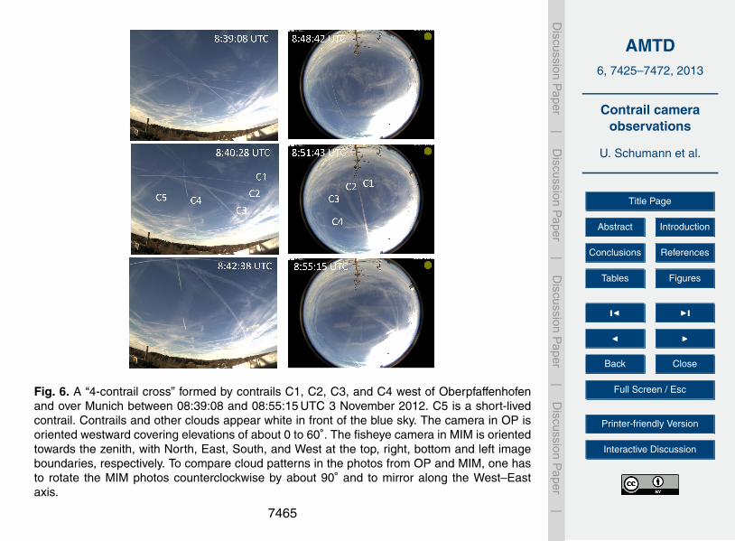
AMTD6, 7425–7472, 2013


U. Schumann et al.

Title Page



Tables Figures

J I

J I

Back Close

Full Screen / Esc



Discussion

Paper

|D

iscussionP

aper|

Discussion

Paper

|D

iscussionP

aper|

Fig. 6. A “4-contrail cross” formed by contrails C1, C2, C3, and C4 west of Oberpfaffenhofenand over Munich between 08:39:08 and 08:55:15 UTC 3 November 2012. C5 is a short-livedcontrail. Contrails and other clouds appear white in front of the blue sky. The camera in OP isoriented westward covering elevations of about 0 to 60◦. The fisheye camera in MIM is orientedtowards the zenith, with North, East, South, and West at the top, right, bottom and left imageboundaries, respectively. To compare cloud patterns in the photos from OP and MIM, one hasto rotate the MIM photos counterclockwise by about 90◦ and to mirror along the West–Eastaxis.

7465





AMTD6, 7425–7472, 2013


U. Schumann et al.

Title Page



Tables Figures

J I

J I

Back Close

Full Screen / Esc



Discussion

Paper

|D

iscussionP

aper|

Discussion

Paper

|D

iscussionP

aper|

Fig. 7. Viewing directions to contrail C1 from cameras OP and MIM at a sequence of times(08:39:08, 42:08, 42:38, 48:42, 51:43, 55:15 UTC, from left to right). The contrail altitude is theresult of the fit described in Sect. 3.2. The contrail x values are the positions where the contrailline cuts the x axis through OP.

7466





AMTD6, 7425–7472, 2013


U. Schumann et al.

Title Page



Tables Figures

J I

J I

Back Close

Full Screen / Esc



Discussion

Paper

|D

iscussionP

aper|

Discussion

Paper

|D

iscussionP

aper|

Fig. 8. Contrail horizontal coordinates (x ,y ; symbols) for contrails C1 to C4 at OP and MIM(times 08:39:08, 42:08, 42:38, 48:42, 51:43, 55:15 UTC) derived from the observations in im-ages from cameras at OP and MIM. The lines show the linear fits to the contrail positions ascomputed from the observed image pixles (X ,Y ) using the camera models (A,E) = F (X ,Y )and the geographic coordinates (x ,y ) = g(A,E ,H) for fitted geometric altitudes z = zC +H a.s.l.Grey lines show lake positions for orientation.

7467





AMTD6, 7425–7472, 2013


U. Schumann et al.

Title Page



Tables Figures

J I

J I

Back Close

Full Screen / Esc



Discussion

Paper

|D

iscussionP

aper|

Discussion

Paper

|D

iscussionP

aper|

Fig. 9. Section of Fig. 6 (red color part), from OP at 08:40:28 UTC, with the 5 contrails C1 toC5, with two grids of geographic x–y lines for orientation, a coarse one (1 km grid spacing)at z = 11 km altitude a.s.l., and a fine one, rotated into flight direction of C5, with 100 m gridspacing, at z = 12 km. The insert in the lower left corner shows contrail C5 and the fine gridenlarged.

7468





AMTD6, 7425–7472, 2013


U. Schumann et al.

Title Page



Tables Figures

J I

J I

Back Close

Full Screen / Esc



Discussion

Paper

|D

iscussionP

aper|

Discussion

Paper

|D

iscussionP

aper|

Fig. 10. Aircraft flight tracks (red lines) in horizontal coordinates (x ,y ) relative to the positionsof the camera in Oberpfaffenhofen (OP, cross) as identified from aircraft waypoint data. Sight-ings of the aircraft (black circles connected with black lines), based on pixel coordinates in thecamera images and traffic data flight altitudes. The single black circles for C2 and C4 denotethe first contrail sighting. The blue lines (linear fits of observed positions) locate the contrailsC1 to C4 at times 08:42:38 and 08:51:43 UTC. Grey lines locate the lakes.

7469





AMTD6, 7425–7472, 2013


U. Schumann et al.

Title Page



Tables Figures

J I

J I

Back Close

Full Screen / Esc



Discussion

Paper

|D

iscussionP

aper|

Discussion

Paper

|D

iscussionP

aper|

��

��

��

��

�

��

��

��

��

��

��

Fig. 11. Top: C1 to C5 contrail observations and computed positions (black lines) in the photo from OP at

8:40:28 UTC. The contrail centers are indicated by dash-dotted lines, the lateral contrail boundaries by solid

lines. Note that for C1 and C5 most of the white contrail cloudin the photo is hidden by the computed position

lines. Bottom: Same contrails (except C5) over MIM at 8:51:43 UTC.

21

Fig. 11. Top panel: C1 to C5 contrail observations and computed positions (black lines) in thephoto from OP at 08:40:28 UTC. The contrail centers are indicated by dash-dotted lines, thelateral contrail boundaries by solid lines. Note that for C1 and C5 most of the white contrailcloud in the photo is hidden by the computed position lines. Bottom panel: same contrails(except C5) over MIM at 08:51:43 UTC.

7470





AMTD6, 7425–7472, 2013


U. Schumann et al.

Title Page



Tables Figures

J I

J I

Back Close

Full Screen / Esc



Discussion

Paper

|D

iscussionP

aper|

Discussion

Paper

|D

iscussionP

aper|

Fig. 12. Contrails C1 to C4 in the view of camera MAY, looking towards southeast, together withcomputed contrails (as in Fig. 11), at 08:56:36 UTC.

7471





AMTD6, 7425–7472, 2013


U. Schumann et al.

Title Page



Tables Figures

J I

J I

Back Close

Full Screen / Esc



Discussion

Paper

|D

iscussionP

aper|

Discussion

Paper

|D

iscussionP

aper|

Fig. 13. Profiles of (a) horizontal wind speeds U, V in East and North directions, (b) relativehumidity over ice RHi and maximum RHi (i.e. homogeneous nucleation limit), (c) temperature,from ECMWF data near OP (11◦ E, 48◦ N), vs. pressure altitude a.s.l. at 09:00 UTC. The sym-bols in (a) denote the wind speeds derived from the camera observations for C4, the circles in(b) symbolize estimated RHi values for observed persistent or short contrails (grey or open) forthe 5 contrails. In (c), TSAC,1 is the Schmidt–Appleman criterion threshold temperature for con-trail formation for the RHi obtained from ECMWF and an overall propulsion efficiency η = 0.3;TSAC,2 is the same for higher η (0.4) and RHi equal to RHimax.

7472





contrail study with ground-based cameras

Documents