contributions of heavy metals from material exposures to
TRANSCRIPT

1
R. Pitt and O. Ogburn Aug 25 2013
Contributions of Heavy Metals from Material Exposures to Stormwater
ContentsIntroduction ................................................................................................................... 2 Trace Heavy Metals in Wet Weather Flows ................................................................. 2
Literature Review: Contaminants Associated with Rooftop and Drainage System Materials ....................................................................................................................... 2
Zinc ........................................................................................................................... 3 Copper ...................................................................................................................... 6 Lead ........................................................................................................................ 11 Cadmium ................................................................................................................. 14 Iron .......................................................................................................................... 16 Aluminum ................................................................................................................ 20
Laboratory Tests and Model Fitting to Predict Metal Releases from Material Exposures .................................................................................................................. 20
Modeling the Effects of Material Type, Exposure Time, pH, and Salinity on Metal Releases and Toxicity ............................................................................................. 21
Predictive Models of Metal Releases from Different Pipe and Gutter Materials ......... 28 Chemical Speciation Modeling of Heavy Metals (Medusa Water Chemistry Modeling Environment) .............................................................................................................. 30
Washdown Tests of Exposed Materials at Naval Facilities ..................................... 39 Aluminum ................................................................................................................ 57 Cadmium ................................................................................................................. 67 Copper .................................................................................................................... 73 Iron .......................................................................................................................... 85 Lead ........................................................................................................................ 95 Zinc ....................................................................................................................... 105
Summary of Washoff Tests ...................................................................................... 117 Contaminated Soils Analyses at Navy Facilities .................................................... 119 Comparison of Recent Navy Facility Source Area Water Quality Observations with Other Data (WinSLAMM Calibration File Preparation) ........................................... 120 Trace Heavy Metal Treatability ................................................................................. 126
Summary of Heavy Metal Treatability ....................................................................... 132 References ................................................................................................................. 134

2
Introduction This report section reviews the contributions of selected heavy metals from different materials exposed to rain or runoff. This information is being used to assist in the calibration of WinSLAMM for naval facilities to account for the contributions of these materials exposed at various locations. The section starts with a review of an extensive literature review that was recently conducted by Olga Ogburn during her PhD research at the University of Alabama. Much of the literature focusses on roofing materials and galvanized metals. Her leaching test results of different pipe and tank materials are also summarized. Washdown tests conducted by SPAWAR personnel during this project are also summarized in this section. An overall summary of these data was also prepared for an overview of the most critical exposed materials and likely concentrations and loss rates. The treatability of stormwater heavy metals is also briefly discussed based on their characteristics as observed during these tests and from the literature. The most important characteristics affecting treatability include: concentrations, filterable fraction, likely complexation, ionic state, and associations with different particle sizes. Trace Heavy Metals in Wet Weather Flows The material in the literature review and leach test sections are summarized from the research conducted by Dr. Olga Ogburn as part of her dissertation research: Ogburn, Olga. Ph.D. Urban Stormwater Contamination Associated with Gutter and Pipe Material Degradation. Department of Civil, Construction, and Environmental Engineering at the University of Alabama. 2013. This research was mostly funded by the National Science Foundation (grant no. EPS-0447675). The NSF project included tasks conducted at UA supporting the Center for Optical Sensors and Spectroscopies (COSS) at UAB’s Department of Physics by applying emerging technologies to solve current environmental problems. This research investigated pipe and tank material sources of heavy metals in wet weather flows, to supplement the large amount of available information concerning roof runoff degradation (along with their chemical characteristics and associated treatability). This section shows that many of the heavy metals in stormwater could be related to material selection and that use of proper materials could result in decreased heavy metals in wet weather flows. This section presents the results of a literature review of heavy metal releases from different materials (mostly roofing types) and the results of several controlled leaching tests that examined a variety of roof gutter, piping, and storage tank materials. Literature Review: Contaminants Associated with Rooftop and Drainage System Materials Roofing drainage systems are often made of metallic materials or may have metals as components, including aluminum, zinc, and copper. Researchers have determined these heavy metals are common contaminants in roof runoff at potentially high

3
concentrations (Clark, et al. 2008 a, b; Wallinder 2001; Pitt, et al. 1995; Förster 1996; Morquecho 2005; Tobiason 2004). The metal’s chemical forms (speciation) are determined by such factors as pH, temperature, and inorganic and organic anionic complexation. The presence of other cations in the water also influences metal bioaccumulation and toxicity (US EPA 2007a; Morquecho 2005). The following includes summary tables containing observed concentrations from the different monitoring studies associated with material exposure. Zinc When exposed to the atmosphere, metal material surfaces are in contact with many forms of moisture (condensed water from high humidity, rain, mist, dew, or melting snow) and the materials undergo corrosion (oxidation) processes (Veleva, et al. 2007). When zinc material is exposed to the atmosphere, a protective patina layer (zinc oxides/hydroxides/carbonates) is formed, which serves as a physical barrier between the metal surface and the atmosphere, slowing down further oxidation (Legault and Pearson 1978; Zhang 1996). The patina can be removed physically by winds and sand erosion or by partial dissolution of some soluble patina components when exposed to rain or water condensation on the metal surface, re-exposing the material to continued oxidation. Zinc runoff can lead to zinc accumulations in the soils, and in surface and ground waters (Veleva, et al. 2007). In urban areas, the highest zinc runoff concentrations are found in runoff from roofs having galvanized steel components (such as roofing sheets, flashing, or gutters and downspouts) (Burton and Pitt 2002; Förster 1999; Bannerman, et al. 1983; Pitt, et al. 1995). The following table summarizes zinc concentrations or runoff yields from different materials reported by various researchers.

4
Zinc releases from various sources (Ogburn 2013) Materials Test conditions Zn
concentrations or runoff yields
Reference
Uncoated Galvanized Steel Roofing Materials New uncoated galvanized steel roof
4 mo field test. Pilot Scale. Harrisburg, PA.
3.5 and 9.8 mg/L Clark, et al. (2008a)
Galvanized metal roof
Field Seattle 0.09 and 0.48 mg/L Tobiason and Logan (2000)
Hot dip galvanized steel
2 year field test. The Gulf of Mexico
6.52– 7.98 g m-2 during the 1st year
2.70 and 3.28 g m-2 during the 2nd year
Veleva, et al. (2010)
Hot dip galvanized steel panel
Stockholm, Sweden. 1 year test
2.7 g/m2 per year Wallinder, et al. (2001)
Hot-dip galvanized steel
5 years pilot scale test. Dubendorf, Switzerland
2.4 g/m2 per year Faller and Reiss (2005)
Galvanized steel roof Stockholm, Sweden. 1 year test.
1.2-5.5 mg/L Heijerick, et al. (2002)
Galvanized material Hannover, Germany, 3 year test
4.51 g/m2 per year Lehmann (1995)
Pure Zn and hot dip galvanized steel
Urban and rural areas. The Gulf of Mexico, 18
mo test
6.5 – 8.5 ± 0.30 g/ m2 per yr.
Veleva, et al. (2007)
14 year old zinc roof Germany, 1 year test 0.3 - 30 mg/L 3.73 g/m2 per year
Schriewer, et al. (2008)
40 year old zinc panel
Stockholm, Sweden. 1 year test
3.5 g/m2 per year Wallinder, et al. (2001)
Zinc roof Filed test. Bayreuth, Germany.
17.6 mg/L Forster (1999)
Zinc roof Stockholm, Sweden. 1 year test.
3.8-4.4 mg/L Heijerick, et al. (2002)
40 years old zinc roof Stockholm, Sweden. 1 year test.
8.4 mg/L Heijerick, et al. (2002)
Zinc materials Stockholm, Sweden. 1 year test.
3.0 - 3.3 g/m/2 per year
He, et al. (2001a)
Zinc sheet (0.07% Ti, 0.17% Cu) panel
1 year field test. Olen, Belgium. Industrial area
4.5 and 5.7 g/m2 per year
Wallinder, et al. (2000)
Clay tiles (70%) + zinc sheets, zinc sheets; roofs and gutters
Field test. Central Paris. July 1996 and May 1997
0.8 - 38 mg/L Gromaire-Mertz, et al. (1999)
Zinc gutters Filed test. Bayreuth, Germany.
2-4 mg/L Forster (1999)
zinc roofing Paris, France. 10 mo. test 34 - 64 metric tons per year for City
Gromaire, et al. (2002)

5
Zinc releases from various sources (Ogburn 2013), continued Coated Galvanized Steel Roofing Materials
New coated galvanized metal roof
4 mo field test. Pilot Scale. Harrisburg,
PA
< 0.5 mg/L Clark, et al. (2008a)
60 years old painted galvanized metal roof in the field
Leaching test in the lab
5 - 30 mg/L Clark, et al. (2008b)
60 years old painted galvanized metal roof stored in the barn
Leaching test in the lab
5 - 30 mg/L Clark, et al. (2008b)
Prepainted galvanized steel panel
Stockholm, Sweden. 1 year test
0.07 g/m2 per year
Wallinder, et al. (2001)
Zinc with different surface treatment
5 years pilot scale test. Dubendorf,
Switzerland
1.9 to 3.2 g/m2 per year
Faller and Reiss (2005)
Prepatinated zinc 5 years pilot scale test. Dubendorf,
Switzerland
3.2 g/m2 per year
Faller and Reiss (2005)
Prepainted galvanized steel roof
Stockholm, Sweden. 1 year
test.
0.16-0.63 mg/L Heijerick, et al. (2002)
Uncoated Galvanized Aluminum Roofing Materials Galvalume roofs Pilot-scale scale in
Austin, Texas. Several rain events
in 2010
0.208 – 0.852 mg/L during the
first flush; 0.077 – 0.362 mg/L for later
samples
Mendez, et al. (2011)
Galvalume roof Stockholm, Sweden. 1 year
test.
0.6-1.6 mg/L Heijerick, et al. (2002)
Unpainted Galvalume roof
Field 0.42 - 14.7 mg/L Tobiason (2004)
Coated Galvanized Aluminum Roofing Materials Kynar®-coated Galvalume®
Full scale in Austin, Texas. Several rain
events in 2010
0.098 – 0.179 mg/L during first
flush, 0.058 – 0.177 mg/L for later samples
Mendez, et al. (2011)
New prepainted 55% aluminum-zinc alloy coated steel (Galvalume) roof
2 years field test. Pilot Scale.
Harrisburg, PA
<0.25 mg/L Clark, et al. (2008b)

6
Zinc releases from various sources (Ogburn 2013), continued Other Roofing Materials
Black phosphatated titanium-zinc
5 years pilot scale test. Dubendorf,
Switzerland
1.9 g/m2 per year
Faller and Reiss (2005)
Titanium-zinc sheet after 5 years exposure
5 years pilot scale test. Dubendorf,
Switzerland
2.6 g/m2/year Faller and Reiss (2005)
Aluminum, stainless steel and titanium
5 years pilot scale test. Dubendorf,
Switzerland
< detection limit (0.01 mg/L)
Faller and Reiss (2005)
Polyester roof Zurich, Switzerland. 2 year test
<0.160 mg/L Zobrist, et al. (2000)
Gravel roof Zurich, Switzerland. 2 year test
<0.035 mg/L Zobrist, et al. (2000)
Drinking Water Distribution Systems (DWDS) At the tap after galvanized metal parts in distribution systems
St. Maarten Island, Netherlands
0.006 to 2.29 mg/L (average of
0.19 mg/L)
Gumbs and Dierberg (1985)
DWDS made of asbestos, polyethylene, and iron pipes; piping system materials in houses and buildings were galvanized
DWDS in Zarrinshahr, Iran
0.73*10-3 - 5.80*10-3 mg/L
Shahmansouri, et al. (2003)
DWDS made of asbestos, polyethylene, and iron pipes; piping system materials in houses and buildings were galvanized
DWDS in Mobarakeh, Iran
0.20 *10-3 - 5.80*10-3 mg/L
Shahmansouri, et al. (2003)
The largest sources of zinc in stormwater runoff are galvanized materials, such as zinc-based roofing materials, galvanized roof drainage systems, and galvanized pipes. Galvanized materials have a large potential for contributing zinc to runoff during their useful life. Zinc runoff yields were generally observed to increase with the age of the material. Zinc concentrations in runoff from galvanized materials ranged from 100’s of µg/L to 10’s of mg/L. Zinc concentrations in roof runoff samples frequently exceeded the water quality criteria established by the U.S. EPA and regulatory agencies from other countries. Copper Clark, et al. (2008 a and b) monitored runoff from a pilot-scale selection of roofing materials and other materials at the campus of Penn State Harrisburg for 2 years under natural rain conditions. The copper concentrations from non-copper metal and vinyl

7
materials did not exceed 25 µg/L (a typical toxicant value for certain aquatic plants). The results from laboratory leaching tests showed that copper concentrations may continue to leach out in an acid rain environment during the material’s useful life (Clark, et al. 2008b). For fresh copper sheet, cuprite (Cu2O) was the main crystalline patina constituent during the first 12 weeks of exposure, followed by the formation of paratacamite (Cu2(OH)3Cl) after that exposure period. Formation of paratacamite was a result of significantly higher deposition rates of chlorides between 12 and 26 weeks. After months of atmospheric exposure, basic copper compounds like (Cu2(OH)3Cl), brochantite (Cu4SO4(OH)6) and cuprite (Cu2O) and Posnjakite (Cu4SO4(OH)6
.H2O) can be formed depending on the contamination in the environment (Sandberg et. al. 2006; Faller and Reiss 2005; Kratschmer, et al. 2002). Brochantite (Cu4SO4(OH)6) and posnjakite (Cu4SO4(OH)6
.H2O) are common compounds in sulfate containing environments; (Cu2(OH)3Cl) are often found in chloride rich environments (Kratschmer, et al. 2002). The brochantite phase was still detected after one year of exposure (Sandberg, et al. 2006). The bioavailable portion (available for uptake by an organism) of the released copper was a small fraction (14–54%) of the total copper concentration due to Cu complexation with organic matter in impinging seawater aerosols (Sandberg, et al. 2006). The following table summarizes copper concentrations and runoff yields from different materials reported by various researchers.

8
Copper Releases from Various Sources (Ogburn 2013) Material Test descriptions Cu
concentrations or runoff yields
Reference
Uncoated Copper Roofing Materials Copper roof 2 year field test.
Stockholm, Sweden Average 1.3 - 1.5 g/m2/year
Wallinder, et al. (2000)
Copper roof Stockholm, Sweden. 2 year test
1.3 g/m2/year Faller and Reiss (2005)
Fresh copper sheet Brest, France. 1 year test
1.5 g/m2/year Sandberg, et al. (2006)
Untreated rolled copper sheet
Dubendorf, Switzerland. 5 year
test
1.3 g/m2/year Faller and Reiss (2005)
After copper roof and cast iron and concrete downspouts
Field. Suburban Farsta, Stockholm. Several rains during
2006-2008
5-101 µg/L (median 15
µg/L)
Wallinder, et al. (2009)
After copper roof and cast iron and concrete downspouts and concrete drain system pipe
Field. Suburban Farsta, Stockholm
.Several rains during 2006-2008
2 -175 µg/L (median 18
µg/L)
Wallinder, et al. (2009)
Copper material (salt spray) Medellin, Colombia. 1 year test
16.0 g/m2/year mass loss
Corvo, et al. (2005)
Copper material (salt spray) Havana, Cuba. 1 year test
32.8 g/m2/year mass loss
Corvo, et al. (2005)
Copper material (natural conditions) Havana, Cuba. 1 year
test
9.4 g/m2/year mass loss
Corvo, et al. (2005)
Copper materials Stockholm, Sweden 1.0 - 2.0 g/m2/year
He, et al. (2001a)

9
Copper Releases from Various Sources (Ogburn 2013), continued Other Roofing Materials
Pilot-scale Galvalume roofs
Austin, Texas. Several rain events in 2010
<0.63 - 9.88 µg/L during first flush; <0.63 - 4.84 µg/L for later samples
Mendez, et al. (2011)
Full-scale Kynar®-coated Galvalume® roof
Austin, Texas. Several rain events in 2010
<0.02 µg/L Mendez, et al. (2011)
New uncoated galvanized steel roof
4 mo. Field test. Pilot Scale. Harrisburg, PA
< 3µg/L Clark, et al. (2008a)
Clay tiles, clay tiles (70%) + zinc sheets, zinc sheets, and slate
Central Paris. July 1996 and May 1997
3 - 247 µg/L (median 37
µg/L)
Gromaire-Mertz, et al. (1999)
Metal and vinyl materials panels
4 mo. Field test. Pilot Scale. Harrisburg, PA
< 25 µg/L Clark, et al. (2008a)
New vinyl roof 14 mo. Field test. Pilot Scale. Harrisburg, PA
< 20 µg/L Clark, et al. (2007)
Tile roof Zurich, Switzerland. 14 rain events
400 and 50 µg/L; average 1623 µg/m2
Zobrist, et al. (2000)
New asphalt shingles roof
4 mo. Field test. Pilot Scale. Harrisburg, PA
25 µg/L (median)
112 µg/L (75th percentile
Clark, et al. (2008a)
Tar-covered roofs Washington 166 µg/L Good (1993) New cedar shakes roof 4 mo. Field test. Pilot
Scale. Harrisburg, PA from 1,500 to 27,000 µg/L
Clark, et al. (2008a)

10
Copper Releases from Various Sources (Ogburn 2013), continued Aged/Patinated Copper Materials
Naturally patinated copper sheet
Brest, France. 1 year test
1.3 g/m2/year Sandberg, et al. (2006)
Naturally aged copper roof
Field. Suburban Stockholm, Sweden. Several rains during
2006-2008
0.74 - 1.6 g/m2/year
(median 1.0 g/m2/year)
Wallinder, et al. (2009)
Naturally patinated copper of varying age
Field. Stockholm, Sweden
1.0 - 1.5 g/m2/year
Karlen, et al. (2002)
Naturally patinated copper of varying age
Field. Stockholm, Sweden
900 - 9700 µg/L Karlen, et al. (2002)
Fresh and brown prepatinated copper roofs
Stockholm, Sweden 1.1-1.6 g/m2/year
Wallinder, et al. (2002a)
Fresh and brown prepatinated copper roofs
Singapore 5.5-5.7 g/m2/year
Wallinder, et al. (2002a)
130 years old copper roof sheet and green prepatinated copper sheet
Singapore, Stockholm 1.6-2.3 g/m2/year
Wallinder, et al. (2002a)
Green pre-patinated copper roof sheet
Singapore 8.4-8.8 g/m2/year
Wallinder, et al. (2002a)
Copper Pipes Copper pipes 200 - 800 µg/L Dietz, et al.
(2007) New copper drains Zurich, Switzerland. 14
rain events 7.8 g/(m2 y1) Zobrist, et al.
(2000) 15 - year old drains Zurich, Switzerland. 14
rain events 3.5 g/(m2 y 1) Zobrist, et al.
(2000) Copper facade 1 year test 103 – 104 µg/L Boller and
Steiner (2002) As expected, the highest copper runoff rates were noted from exposed copper materials. Copper-based paints can also be a significant source of copper in runoff. Some studies indicated relatively constant copper runoff yields with time during 5 years of exposure. However, other studies found that new copper materials had higher copper runoff yields compared to older copper materials. Galvanized steel, vinyl, and galvalume materials had copper runoff concentrations that were less than 25 µg/L. The major portion of the copper in the runoff at the source was in the most bioavailable form (hydrated cupric ion), but when the stormwater runoff passes through cast iron and concrete drainage systems, copper may be retained or form complexes with organic matter and change chemical speciation to less toxic or less bioavailable forms.
11
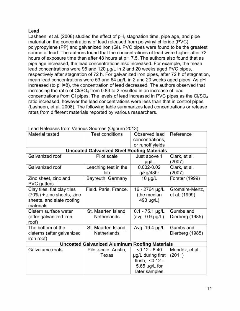
Lead Lasheen, et al. (2008) studied the effect of pH, stagnation time, pipe age, and pipe material on the concentrations of lead released from polyvinyl chloride (PVC), polypropylene (PP) and galvanized iron (GI). PVC pipes were found to be the greatest source of lead. The authors found that the concentrations of lead were higher after 72 hours of exposure time than after 48 hours at pH 7.5. The authors also found that as pipe age increased, the lead concentrations also increased. For example, the mean lead concentrations were 95 and 120 µg/L in 2 and 20 weeks aged PVC pipes, respectively after stagnation of 72 h. For galvanized iron pipes, after 72 h of stagnation, mean lead concentrations were 53 and 64 µg/L in 2 and 20 weeks aged pipes. As pH increased (to pH=8), the concentration of lead decreased. The authors observed that increasing the ratio of Cl/SO4 from 0.83 to 2 resulted in an increase of lead concentrations from GI pipes. The levels of lead increased in PVC pipes as the Cl/SO4 ratio increased, however the lead concentrations were less than that in control pipes (Lasheen, et al. 2008). The following table summarizes lead concentrations or release rates from different materials reported by various researchers. Lead Releases from Various Sources (Ogburn 2013) Material tested Test conditions Observed lead
concentrations, or runoff yields
Reference
Uncoated Galvanized Steel Roofing Materials Galvanized roof Pilot scale Just above 1
µg/L Clark, et al. (2007)
Galvanized roof Leaching test in the lab
0.002-0.02 g/kg/48hr
Clark, et al. (2007)
Zinc sheet, zinc and PVC gutters
Bayreuth, Germany 10 µg/L Forster (1999)
Clay tiles, flat clay tiles (70%) + zinc sheets, zinc sheets, and slate roofing materials
Field. Paris, France. 16 - 2764 µg/L (the median 493 µg/L)
Gromaire-Mertz, et al. (1999)
Cistern surface water (after galvanized iron roof)
St. Maarten Island, Netherlands
0.1 - 75.1 µg/L (avg. 0.9 µg/L).
Gumbs and Dierberg (1985)
The bottom of the cisterns (after galvanized iron roof)
St. Maarten Island, Netherlands
Avg. 19.4 µg/L Gumbs and Dierberg (1985)
Uncoated Galvanized Aluminum Roofing Materials Galvalume roofs Pilot-scale. Austin,
Texas <0.12 - 6.40
µg/L during first flush, <0.12 - 5.65 µg/L for later samples
Mendez, et al. (2011)
12
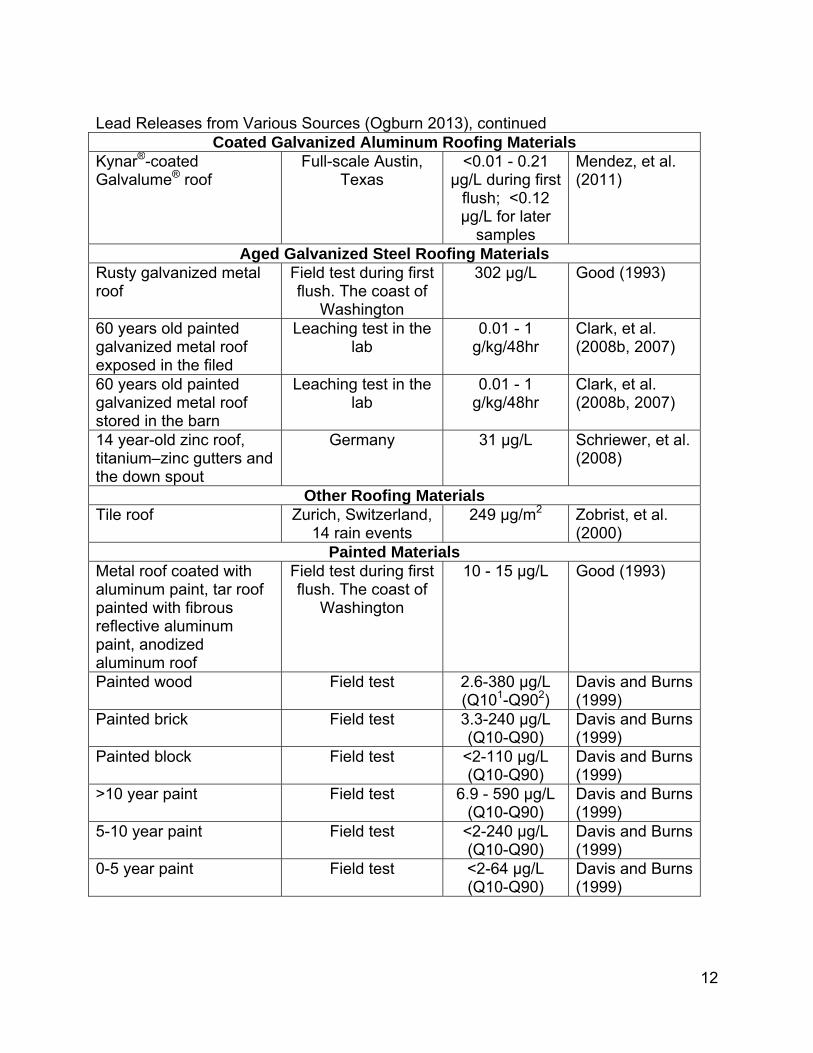
Lead Releases from Various Sources (Ogburn 2013), continued
Coated Galvanized Aluminum Roofing Materials Kynar®-coated Galvalume® roof
Full-scale Austin, Texas
<0.01 - 0.21 µg/L during first
flush; <0.12 µg/L for later
samples
Mendez, et al. (2011)
Aged Galvanized Steel Roofing Materials Rusty galvanized metal roof
Field test during first flush. The coast of
Washington
302 µg/L Good (1993)
60 years old painted galvanized metal roof exposed in the filed
Leaching test in the lab
0.01 - 1 g/kg/48hr
Clark, et al. (2008b, 2007)
60 years old painted galvanized metal roof stored in the barn
Leaching test in the lab
0.01 - 1 g/kg/48hr
Clark, et al. (2008b, 2007)
14 year-old zinc roof, titanium–zinc gutters and the down spout
Germany 31 µg/L Schriewer, et al. (2008)
Other Roofing Materials Tile roof Zurich, Switzerland,
14 rain events 249 µg/m2 Zobrist, et al.
(2000) Painted Materials
Metal roof coated with aluminum paint, tar roof painted with fibrous reflective aluminum paint, anodized aluminum roof
Field test during first flush. The coast of
Washington
10 - 15 µg/L Good (1993)
Painted wood Field test 2.6-380 µg/L (Q101-Q902)
Davis and Burns (1999)
Painted brick Field test 3.3-240 µg/L (Q10-Q90)
Davis and Burns (1999)
Painted block Field test <2-110 µg/L (Q10-Q90)
Davis and Burns (1999)
>10 year paint Field test 6.9 - 590 µg/L (Q10-Q90)
Davis and Burns (1999)
5-10 year paint Field test <2-240 µg/L (Q10-Q90)
Davis and Burns (1999)
0-5 year paint Field test <2-64 µg/L (Q10-Q90)
Davis and Burns (1999)

13
Lead Releases from Various Sources (Ogburn 2013), continued Drinking Water Distribution Systems
Galvanized iron pipe after 2 weeks of use, 72 hr of stagnation
increasing the ratio of Cl/SO4 from 0.83
to 2
58 µg/L Lasheen, et al. (2008)
Galvanized iron pipe after 20 weeks of use, 72 hr of stagnation
increasing the ratio of Cl/SO4 from 0.83
to 2
70 µg/L Lasheen, et al. (2008)
PVC pipes after 2 weeks of use, 72 hr of stagnation
pH 7.5 95 µg/L Lasheen, et al. (2008)
PVC pipes after 20 weeks of use, 72 hr of stagnation
pH 7.5 120µg/L Lasheen, et al. (2008)
PVC pipes after 2 weeks of use, 72 hr of stagnation
pH 6 100µg/L Lasheen, et al. (2008)
PVC pipes after 20 weeks of use, 72 hr of stagnation
pH 6 130µg/L Lasheen, et al. (2008)
PVC pipes after 2 weeks of use, 72 hr of stagnation
pH 8 110µg/L Lasheen, et al. (2008)
PVC pipes after 20 weeks of use, 72 hr of stagnation
pH 8 20µg/L Lasheen, et al. (2008)
PVC pipe after 2 weeks of use, 72 hr of stagnation
increasing the ratio of Cl/SO4 from 0.83
to 2
80µg/L Lasheen, et al. (2008)
PVC pipe after 20 weeks of use, 72 hr of stagnation
increasing the ratio of Cl/SO4 from 0.83
to 2
100µg/L Lasheen, et al. (2008)
Unplasticized PVC pipe after 10 h of exposure
- 430µg/L Al-Malack (2001)
Unplasticized PVC pipe after 48 h of exposure
- 780µg/L Al-Malack (2001)
Unplasticized PVC pipe after 48 h of exposure
pH 5 1000µg/L Al-Malack (2001)
Unplasticized PVC pipe after 12 h of exposure
UV exposure 115µg/L Al-Malack (2001)
Unplasticized PVC pipe after 5 days of exposure
UV exposure 312 µg/L Al-Malack (2001)
Unplasticized PVC pipe after 14 days of exposure
UV exposure 799µg/L Al-Malack (2001)

14
Lead Releases from Various Sources (Ogburn 2013), continued PVC, lined cast iron, unlined cast iron, and galvanized steel aged pipes (40+ years)
Phosphorus or SiO2 inhibitor
< 5 µg/L Dietz, et al. (2007)
PVC, lined cast iron, unlined cast iron, and galvanized steel aged pipes (40+ years)
pH control max.65 µg/L Dietz, et al. (2007)
Galvanized piping systems, asbestos,
polyethylene, iron pipes
Pilot scale. Zarrinshahr, Iran
1.60 - 16.00 µg/L (avg. 5.7
µg/L )
Shahmansouri, et al. ( 2003)
Galvanized piping systems, asbestos,
polyethylene, iron pipes
Pilot scale. Mobarakeh, Iran
0.60 - 18.70 µg/L (avg. 7.8
µg/L)
Shahmansouri, et al. ( 2003)
At the tap (after galvanized iron roof, gutter and down spout, distribution system)
St. Maarten Island, Netherlands
0.2-70.0 µg/L (average of 2.1
µg/L)
Gumbs and Dierberg (1985)
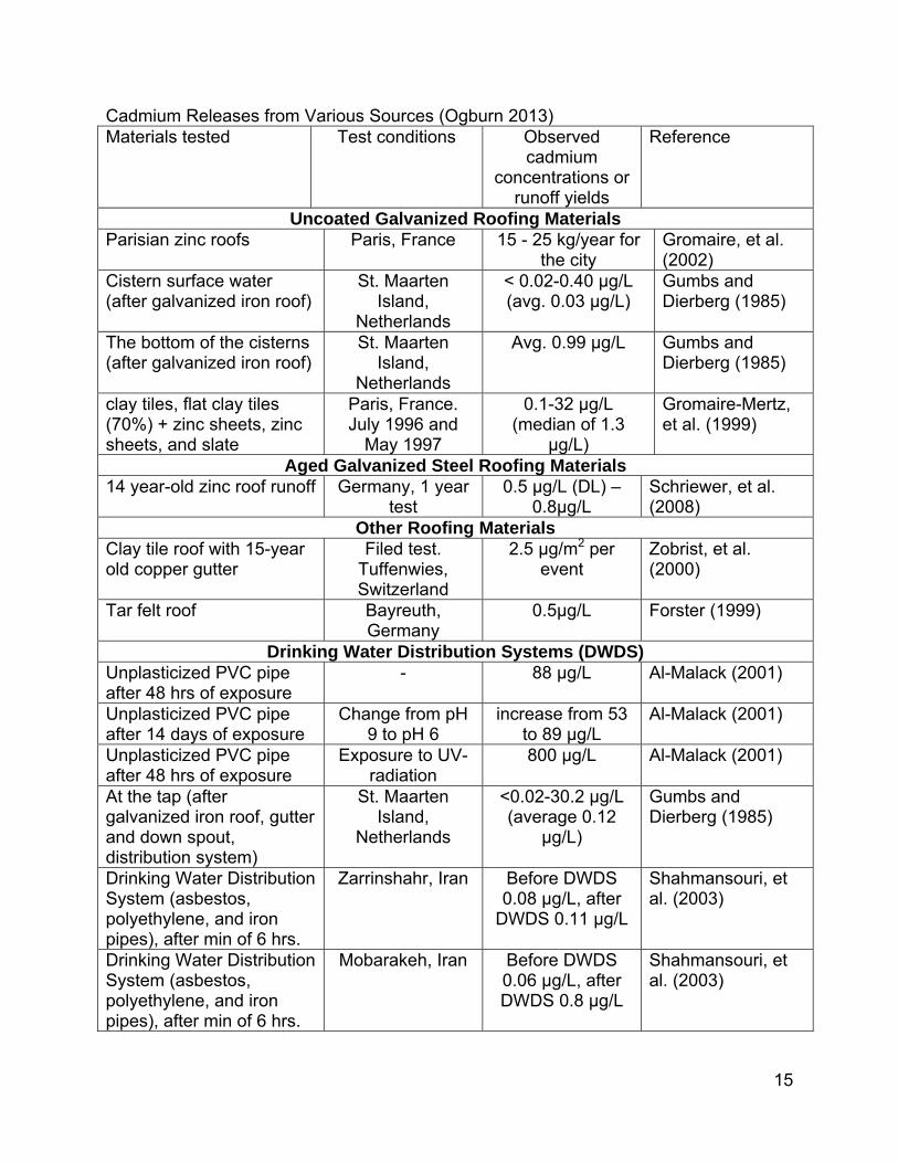
1 and 2 10th and 90th percentiles of data values, respectively Galvanized steel, PVC and unplasticized PVC, galvalume, and zinc materials can be sources of lead concentration increases in water. Lead concentrations released from galvanized steel and PVC materials increase with increased exposure time, increased pipe age, and pH decreases. Also, exposure to UV-radiation was determined to promote the migration of lead from unplasticized PVC pipes. Additionally, painted materials can be a source of lead in stormwater, with lead releases being higher from older types of paints. The rise in the ratio of Cl/SO4 from 0.83 to 2 resulted in an increase in lead concentrations from galvanized iron and PVC pipe exposure. Cadmium Gromaire-Mertz, et al. (1999) examined runoff from different roofing materials and gutters in Paris, France, between July 1996 and May 1997. Roofing materials included clay tiles, zinc sheets, and slate. Cadmium concentrations in roof runoff (1 to 5 µg/L) were below the level 2 water quality criteria (1,000 µg/L) with the exception of runoff from the zinc sheet roof runoff samples. Cadmium concentrations were extremely high in roof runoff from the zinc roofs. Leaching of cadmium is explained by the erosion of the zinc roofing material, in which cadmium is a minor constituent. Förster (1996) found that generally, the dissolved fraction of cadmium was greater than the particulate fraction for roof runoff. The following table summarizes cadmium concentrations and release rates from different materials reported by various researchers.
15
Cadmium Releases from Various Sources (Ogburn 2013) Materials tested Test conditions Observed
cadmium concentrations or
runoff yields
Reference
Uncoated Galvanized Roofing Materials Parisian zinc roofs Paris, France 15 - 25 kg/year for
the city Gromaire, et al. (2002)
Cistern surface water (after galvanized iron roof)
St. Maarten Island,
Netherlands
< 0.02-0.40 µg/L (avg. 0.03 µg/L)
Gumbs and Dierberg (1985)
The bottom of the cisterns (after galvanized iron roof)
St. Maarten Island,
Netherlands
Avg. 0.99 µg/L Gumbs and Dierberg (1985)
clay tiles, flat clay tiles (70%) + zinc sheets, zinc sheets, and slate
Paris, France. July 1996 and
May 1997
0.1-32 µg/L (median of 1.3
µg/L)
Gromaire-Mertz, et al. (1999)
Aged Galvanized Steel Roofing Materials 14 year-old zinc roof runoff Germany, 1 year
test 0.5 µg/L (DL) –
0.8µg/L Schriewer, et al. (2008)
Other Roofing Materials Clay tile roof with 15-year old copper gutter
Filed test. Tuffenwies, Switzerland
2.5 µg/m2 per event
Zobrist, et al. (2000)
Tar felt roof Bayreuth, Germany
0.5µg/L Forster (1999)
Drinking Water Distribution Systems (DWDS) Unplasticized PVC pipe after 48 hrs of exposure
- 88 µg/L Al-Malack (2001)
Unplasticized PVC pipe after 14 days of exposure
Change from pH 9 to pH 6
increase from 53 to 89 µg/L
Al-Malack (2001)
Unplasticized PVC pipe after 48 hrs of exposure
Exposure to UV-radiation
800 µg/L Al-Malack (2001)
At the tap (after galvanized iron roof, gutter and down spout, distribution system)
St. Maarten Island,
Netherlands
<0.02-30.2 µg/L (average 0.12
µg/L)
Gumbs and Dierberg (1985)
Drinking Water Distribution System (asbestos, polyethylene, and iron pipes), after min of 6 hrs.
Zarrinshahr, Iran Before DWDS 0.08 µg/L, after
DWDS 0.11 µg/L
Shahmansouri, et al. (2003)
Drinking Water Distribution System (asbestos, polyethylene, and iron pipes), after min of 6 hrs.
Mobarakeh, Iran Before DWDS 0.06 µg/L, after DWDS 0.8 µg/L
Shahmansouri, et al. (2003)

16
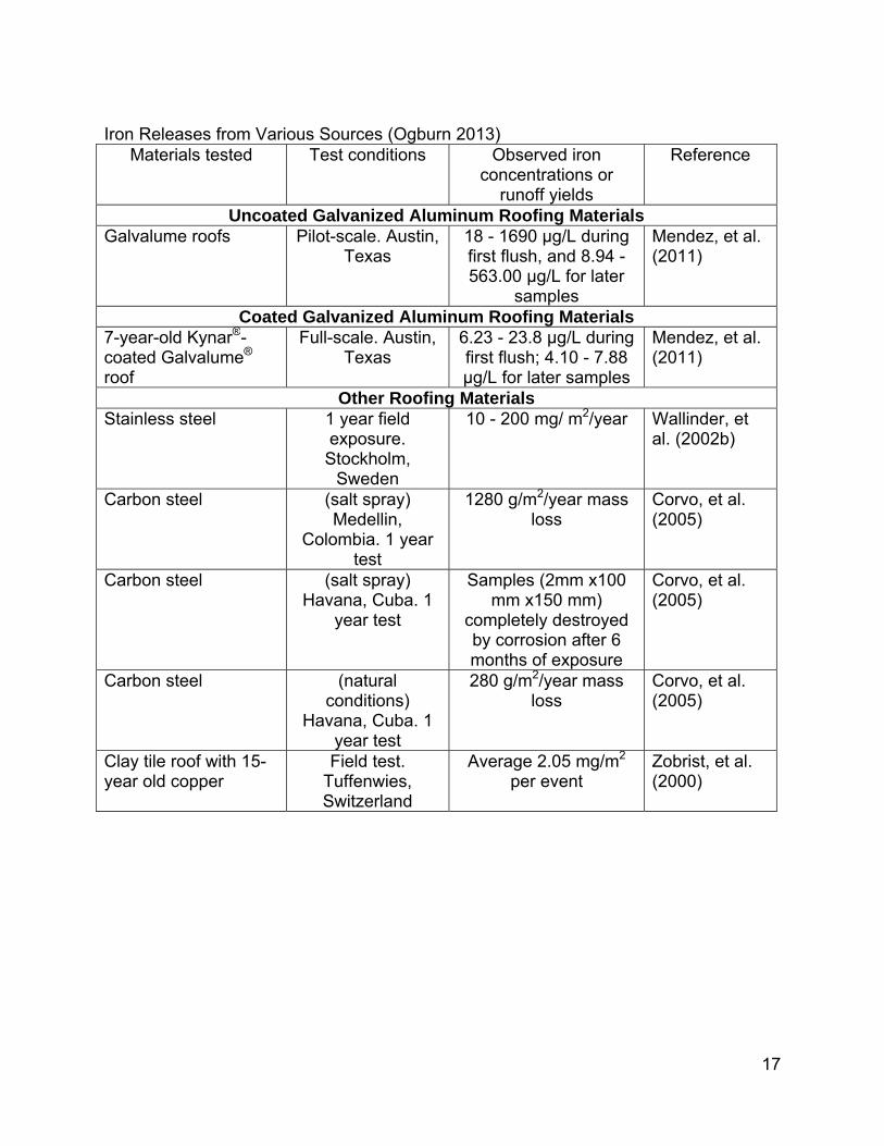
PVC, zinc, tile, tar felt, and galvanized iron materials can all be sources of cadmium in runoff. Exposure to UV-radiation promoted the migration of cadmium stabilizers from unplasticized PVC pipes. A decrease in the pH of the water was also found to increase the cadmium concentrations released from the uPVC pipes. Iron Corrosion of iron is the primary cause of iron release. When metal surfaces are covered with corrosion scales, iron may be released by the corrosion of iron metal, the dissolution of ferrous components of the scales, and hydraulic scouring of particles from the scales (Sarin, et al. 2004). The corrosion rate of clean iron surfaces typically increases with the increase of the oxidant (such as oxygen) concentrations. When scale layers are formed during the corrosion process, they can influence the rate of diffusion of oxygen to the metal, and slow down corrosion. The environment inside the corrosion scales present in water distribution pipes is characterized with highly reducing conditions and high concentrations of Fe (II). Sarin, et al. (2004) also noted that iron releases increased with stagnation time, while the DO concentration diminished. For initial DO concentration of 6.2 mg/L and pH of 8.9, iron releases from the iron pipe were approximatelly100 µg/m of pipe length after 20 hours of stagnation, and reached 375 µg/m of pipe length after 120 hours of stagnation. The following table summarizes iron concentrations and runoff yields from different materials reported by various researchers.
17
Iron Releases from Various Sources (Ogburn 2013)
Materials tested Test conditions Observed iron concentrations or
runoff yields
Reference
Uncoated Galvanized Aluminum Roofing Materials Galvalume roofs Pilot-scale. Austin,
Texas 18 - 1690 µg/L during first flush, and 8.94 - 563.00 µg/L for later
samples
Mendez, et al. (2011)
Coated Galvanized Aluminum Roofing Materials 7-year-old Kynar®-coated Galvalume® roof
Full-scale. Austin, Texas
6.23 - 23.8 µg/L during first flush; 4.10 - 7.88 µg/L for later samples
Mendez, et al. (2011)
Other Roofing Materials Stainless steel 1 year field
exposure. Stockholm,
Sweden
10 - 200 mg/ m2/year Wallinder, et al. (2002b)
Carbon steel (salt spray) Medellin,
Colombia. 1 year test
1280 g/m2/year mass loss
Corvo, et al. (2005)
Carbon steel (salt spray) Havana, Cuba. 1
year test
Samples (2mm x100 mm x150 mm)
completely destroyed by corrosion after 6 months of exposure
Corvo, et al. (2005)
Carbon steel (natural conditions)
Havana, Cuba. 1 year test
280 g/m2/year mass loss
Corvo, et al. (2005)
Clay tile roof with 15-year old copper
Field test. Tuffenwies, Switzerland
Average 2.05 mg/m2 per event
Zobrist, et al. (2000)

18
Iron Releases from Various Sources (Ogburn 2013), continued Drinking Water Distribution Systems (DWDS)
2 weeks aged galvanized iron pipes after 72 h of contact time
Lab test Avg. 0.7 mg/L Lasheen, et al. (2008)
20 weeks aged galvanized iron pipes after 72 h of contact time
Lab test Avg. 1.44 mg/L Lasheen, et al. (2008)
2 weeks aged galvanized iron pipes after 72 h of contact time
pH = 6 Avg. 0.99 mg/L Lasheen, et al. (2008)
20 weeks aged galvanized iron pipes after 72 h of contact time
pH = 6 Avg. 1.65 mg/L Lasheen, et al. (2008)
2 weeks aged galvanized iron pipes after 72 h of contact time
pH = 8 Avg. 1.44 mg/L Lasheen, et al. (2008)
20 weeks aged galvanized iron pipes after 72 h of contact time
pH = 8 Avg. 1.3 mg/L Lasheen, et al. (2008)
Drinking Water Distribution System (asbestos, polyethylene, and iron pipes), after min of 6 hrs.
Zarrinshahr, Iran Before DWDS 0.08 µg/L, after DWDS 0.71
µg/L
Shahmansouri, et al. (2003)
Drinking Water Distribution System (asbestos, polyethylene, and iron pipes), after min of 6 hrs.
Mobarakeh, Iran Before DWDS 0.05 µg/L, after DWDS 0.85
µg/L
Shahmansouri, et al. (2003)
2 weeks aged PVC pipes after 72 h of contact time
Lab test Avg. 0.058 mg/L Lasheen, et al. (2008)
20 weeks aged PVC pipes after 72 h of contact time
Lab test Avg. 0.07 mg/L Lasheen, et al. (2008)

19
Iron Releases from Various Sources (Ogburn 2013), continued 2 weeks aged PVC pipes after 72 h of contact time
pH = 6 Avg. 0.068 mg/L Lasheen, et al. (2008)
20 weeks aged PVC pipes after 72 h of contact time
pH = 6 Avg. 0.08 mg/L Lasheen, et al. (2008)
2 weeks aged PVC pipes after 72 h of contact time
pH = 8 Avg. 0.07 mg/L Lasheen, et al. (2008)
20 weeks aged PVC pipes after 72 h of contact time
pH = 8 Avg. 0.06 mg/L Lasheen, et al. (2008)
2 weeks aged polypropylene pipes after 72 h of contact time
Lab test Avg. 0.06 mg/L Lasheen, et al. (2008)
20 weeks aged polypropylene pipes after 72 h of contact time
Lab test Avg. 0.07 mg/L Lasheen, et al. (2008)
2 weeks aged polypropylene pipes after 72 h of contact time
pH = 6 Avg. 0.073 mg/L Lasheen, et al. (2008)
20 weeks aged polypropylene pipes after 72 h of contact time
pH = 6 Avg. 0.083 mg/L Lasheen, et al. (2008)
2 weeks aged polypropylene pipes after 72 h of contact time
pH = 8 Avg. 0.069 mg/L Lasheen, et al. (2008)
20 weeks aged polypropylene pipes after 72 h of contact time
pH = 8 Avg. 0.06 mg/L Lasheen, et al. (2008)
PVC, polypropylene, galvanized iron, clay tile, polyester, stainless steel, galvanized iron, and Galvalume® metal materials were found to release iron into runoff water. Exposure time had an effect on iron released from PVC, polypropylene, and galvanized iron materials. Greater iron runoff concentrations were observed for aged PVC, polypropylene, and galvanized iron pipes compared to new materials. As pH decreased, iron concentrations leaching from PVC, polypropylene, and galvanized iron, cast iron,
20
and galvanized steel materials increased. High Cl-/SO42- ratios increased iron
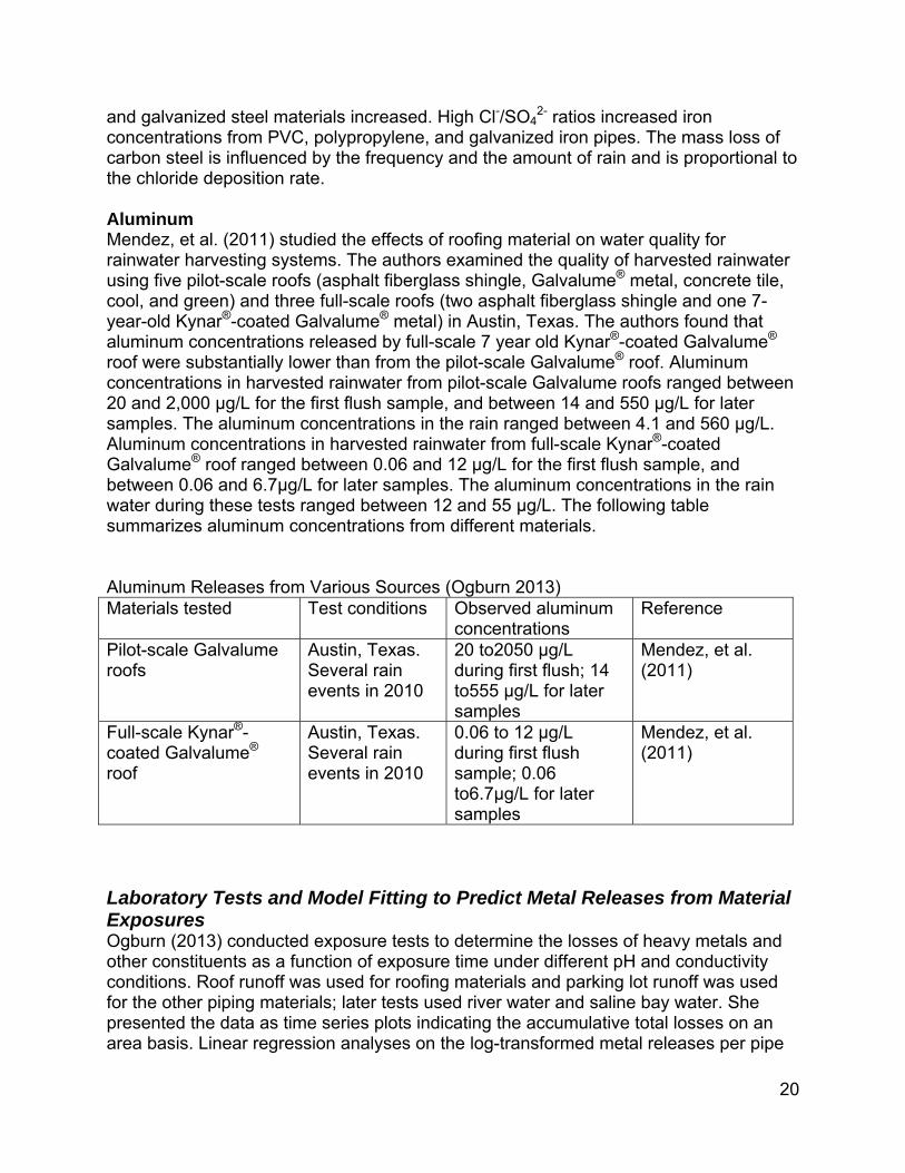
concentrations from PVC, polypropylene, and galvanized iron pipes. The mass loss of carbon steel is influenced by the frequency and the amount of rain and is proportional to the chloride deposition rate. Aluminum Mendez, et al. (2011) studied the effects of roofing material on water quality for rainwater harvesting systems. The authors examined the quality of harvested rainwater using five pilot-scale roofs (asphalt fiberglass shingle, Galvalume® metal, concrete tile, cool, and green) and three full-scale roofs (two asphalt fiberglass shingle and one 7-year-old Kynar®-coated Galvalume® metal) in Austin, Texas. The authors found that aluminum concentrations released by full-scale 7 year old Kynar®-coated Galvalume® roof were substantially lower than from the pilot-scale Galvalume® roof. Aluminum concentrations in harvested rainwater from pilot-scale Galvalume roofs ranged between 20 and 2,000 µg/L for the first flush sample, and between 14 and 550 µg/L for later samples. The aluminum concentrations in the rain ranged between 4.1 and 560 µg/L. Aluminum concentrations in harvested rainwater from full-scale Kynar®-coated Galvalume® roof ranged between 0.06 and 12 µg/L for the first flush sample, and between 0.06 and 6.7µg/L for later samples. The aluminum concentrations in the rain water during these tests ranged between 12 and 55 µg/L. The following table summarizes aluminum concentrations from different materials. Aluminum Releases from Various Sources (Ogburn 2013) Materials tested Test conditions Observed aluminum
concentrations Reference
Pilot-scale Galvalume roofs
Austin, Texas. Several rain events in 2010
20 to2050 µg/L during first flush; 14 to555 µg/L for later samples
Mendez, et al. (2011)
Full-scale Kynar®-coated Galvalume® roof
Austin, Texas. Several rain events in 2010
0.06 to 12 µg/L during first flush sample; 0.06 to6.7µg/L for later samples
Mendez, et al. (2011)
Laboratory Tests and Model Fitting to Predict Metal Releases from Material Exposures Ogburn (2013) conducted exposure tests to determine the losses of heavy metals and other constituents as a function of exposure time under different pH and conductivity conditions. Roof runoff was used for roofing materials and parking lot runoff was used for the other piping materials; later tests used river water and saline bay water. She presented the data as time series plots indicating the accumulative total losses on an area basis. Linear regression analyses on the log-transformed metal releases per pipe

21
surface area vs. log time for different pipe and gutter materials under controlled and natural pH conditions, after supporting statistical analyses were used to identify groupings of the data. The majority of the scatterplots revealed that first order polynomials can be fitted to the log of metal releases vs. log of time. Modeling the Effects of Material Type, Exposure Time, pH, and Salinity on Metal Releases and Toxicity Spearman correlation analyses were used to determine the associations between constituents and the degree of that association, while cluster analyses were conducted to identify more complex relationships between the parameters. Principle component analyses were conducted to identify groupings of parameters having similar characteristics. The significant factors identified from the factorial analyses were used to combine the data into groups. The final model can be used to determine which materials can be safely used for short contact times such as for gutters and pipes, and for longer term storage, such as for tanks. Full 23 Factorial Analyses Full 23 factorial analyses were performed on Cu, Zn, Pb constituents (using the release rates of mg per m2of surface area of exposed materials) and toxicities in percent light reductions at 15 and 45 min of Microtox bacteria exposure times. These analyses therefore examined the effects of time, pH, and material and their interactions for the first testing series data and the effects of time, conductivity, and material and their interactions during for the second testing series. The levels for the different factors defining how the data were organized are shown on the table below. Kruskal-Wallis tests were initially performed for each constituent to determine if the data for 1, 2, and 3 months of pipe and gutter exposure could be used together to represent long term exposure times. The tests indicated that there were no statistically significant differences (at 0.05 significance level) between these data so they were combined into one data category. Kruskal–Wallis tests were also conducted for each constituent on the data after 0.5 and 1h of exposure to indicate if they could be combined to represent short exposure periods. These tests similarly showed that these data could be combined into one category for short term exposure times.

22
23 Factorial Experiment. Factors and levels (Ogburn 2013) Constituent Factors and levels Time pH or Conductivity Material Cu (mg/m2) short (0.5h, 1h) (-) vs. long
(1mo, 2mo,3mo) (+) pH 5 (-) vs. pH8 (+) copper (-) vs. the rest
of the materials (+) Cu (mg/m2) short (1h) (-) vs. long
(1mo, 2mo,3mo) (+) high cond. (-) vs. low cond. (+)
copper (-) vs. the rest of the materials (+)
Zn (mg/m2) short (0.5h, 1h) (-) vs. long (1mo, 2mo,3mo) (+)
pH 5 (-) vs. pH8 (+) galv. steel (-) vs. the rest of the materials (+)
Zn (mg/m2) short (1h) (-) vs. long (1mo, 2mo,3mo) (+)
high cond. (-) vs. low cond. (+)
galv. steel (-) vs. the rest of the materials (+)
Pb (mg/m2) short (0.5h, 1h) (-) vs. long (1mo, 2mo,3mo) (+)
pH 5 (-) vs. pH8 (+) galv. steel (-) vs. the rest of the materials (+)
Pb (mg/m2) short (1h) (-) vs. long (1mo, 2mo,3mo) (+)
high cond. (-) vs. low cond. (+)
galv. steel (-) vs. the rest of the materials (+)
The factorial effect/pooled standard error ratio of the factorial analysis were used to determine whether or not the data could be combined into groups for each constituent based on the effect (or absence of effect) of the factors and their interactions. The ratios of Effect/SE that were greater than three are highlighted in red, and those that are greater than five are highlighted in bold red, indicating likely significant factors and interactions. For each constituent, effects and their interactions were sorted into significant, marginally significant, and not significant groups, according to the absolute values of their effects. Combined Data Group Analyses The following figures show metal releases for the combined data groups, based on the prior analyses. The significant factors and their interactions from 23 factorial analyses were used for grouping the samples and conditions. The box plots were constructed only for the groups that were found to be significant. Group box plots were plotted for these constituents to illustrate the variations and differences between each group. The group box plot of copper releases compares the copper material samples with the all of the other samples for pH 5 and 8 conditions during both short and long exposure times. Full 23 factorial analyses showed that the three-way interaction of pH x material x time was significant, therefore the main effects should not be interpreted separately (Navidi 2006).The data was combined into the groups according to the interaction of pH, material, and time. Copper materials were the most significant source of copper, as expected. Lower pH conditions increased the copper releases from the copper materials. The copper releases in the sample groups of all materials increased with exposure time. The combination of conditions, such as copper materials under pH 5 water conditions during short exposure time, significantly increased copper releases. Similarly, copper releases increased dramatically for copper materials immersed into pH 5 water for long exposure periods, as well as for copper materials immersed into pH 8 waters for long exposure periods. The groups combining the rest of the materials for pH 5 and pH 8 conditions during short exposure time into one group is also shown, with the

23
rest of the materials for pH 5 and pH 8 conditions during long exposure time combined into one group.
Copper Release. Controlled pH.
Material and Condition
Cop.5.S
.
Cop.8.S
.
Cop.5.L
.
Cop.8.L
.
The re
st.5
,8.S
The re
st.5
,8.L
Co
pp
er
Re
leas
e (
log
(m
g/m
^2
))
0.01
0.1
1
10
100
1000
Group box plot for copper release in mg/m2 for materials immersed in pH 5 and pH 8 waters (Ogburn 2013).
The following figure shows copper releases in the pipe and gutter samples immersed in bay and river waters. Copper releases were detected during both short and long exposures for controlled pH conditions and for both the natural bay and river water tests. Copper concentrations were greater for bay water exposure tests compared to river water exposure tests. Exposure time also increased copper releases in the samples with copper gutter materials. The combination of copper materials, high conductivity, and long exposure periods, as well as copper materials, low conductivity, and long exposure periods, significantly increased copper releases.
5 = pH 5 8 = pH 8 S = short exposure time L = long exposure

24
Copper Release. Natural pH.
Material & Condition
Cop.B.S
.
Cop.R.S
.
Cop.B.L
.
Cop.R.L
.
The re
st.B
,R.S
,L.
Cop
per
Rel
ease
(lo
g (m
g/m
^2))
0.1
1
10
100
1000
10000
Group box plot for copper release in mg/m2 for materials immersed in bay and river waters (Ogburn 2013).
The following figure is a group box plot of zinc releases for the galvanized steel samples compared to the rest of the material samples for pH 5 and8 conditions during short and long exposure periods. Galvanized steel materials were the greatest source of zinc. During short exposure times, low pH conditions increased zinc releases in the samples with galvanized materials, however during long exposure times, zinc releases were greater under controlled pH 8 conditions compared to controlled pH 5 conditions. Exposure time increased zinc releases in the samples with galvanized materials. The combination of such factors as galvanized materials, pH 5 resulted in significant increases in zinc releases during the short exposure periods. Similarly, zinc releases were much higher for galvanized materials immersed into pH 5 waters for long exposure
B = bay R = river S = short exposure time L = long exposure

25
periods, and for galvanized materials immersed into pH 8 waters for long exposure periods. The other figure shows “the rest” of the materials at pH 5 and pH 8 conditions during short and long exposure periods combined into one group.
Zinc Releases. Controlled pH
Material & Condition
Galv.
5.S.
Galv.
8.S.
Galv.
5.L.
Galv.
8.L.
The re
st.5
,8.S
.L.
Zin
c R
elea
ses
(lo
g (
mg
/m^
2))
0.1
1
10
100
1000
10000
Group box plot for zinc release in mg/m2 for materials immersed in pH 5 and pH 8
waters (Ogburn 2013).
Zinc releases also increased with exposure time for galvanized steel pipes and gutters immersed in bay and river waters. In this example, the interaction of material and exposure time was significant. Galvanized materials exposed to natural pH waters resulted in elevated zinc releases even during short periods. The combination of galvanized materials exposed to natural pH waters for long periods further increased zinc releases.
5 = pH 5 8 = pH 8 S = short exposure time L l

26
Zinc Releases. Natural pH.
Material & Condition
Galv.S Galv.L The rest.S,L
Zin
c R
elea
se (
log
(m
g/m
^2)
)
1e-1
1e+0
1e+1
1e+2
1e+3
1e+4
1e+5
Group box plot for zinc release in mg/m2 for materials immersed in bay and river waters
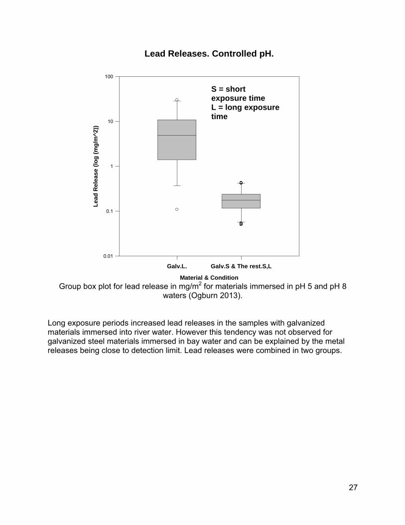
(Ogburn 2013). Galvanized steel materials were the only source of lead releases detected. For lead releases under controlled pH conditions, there was a difference between the groups of galvanized materials during long exposure times and the group of galvanized materials during short exposure times and the rest of the materials during both short and long exposure times. Under controlled pH conditions, lead releases significantly increased for galvanized materials and long exposure periods.
S = short exposure time L = long exposure time
27
Lead Releases. Controlled pH.
Material & Condition
Galv.L. Galv.S & The rest.S,L
Lea
d R
elea
se (
log
(m
g/m
^2)
)
0.01
0.1
1
10
100
Group box plot for lead release in mg/m2 for materials immersed in pH 5 and pH 8
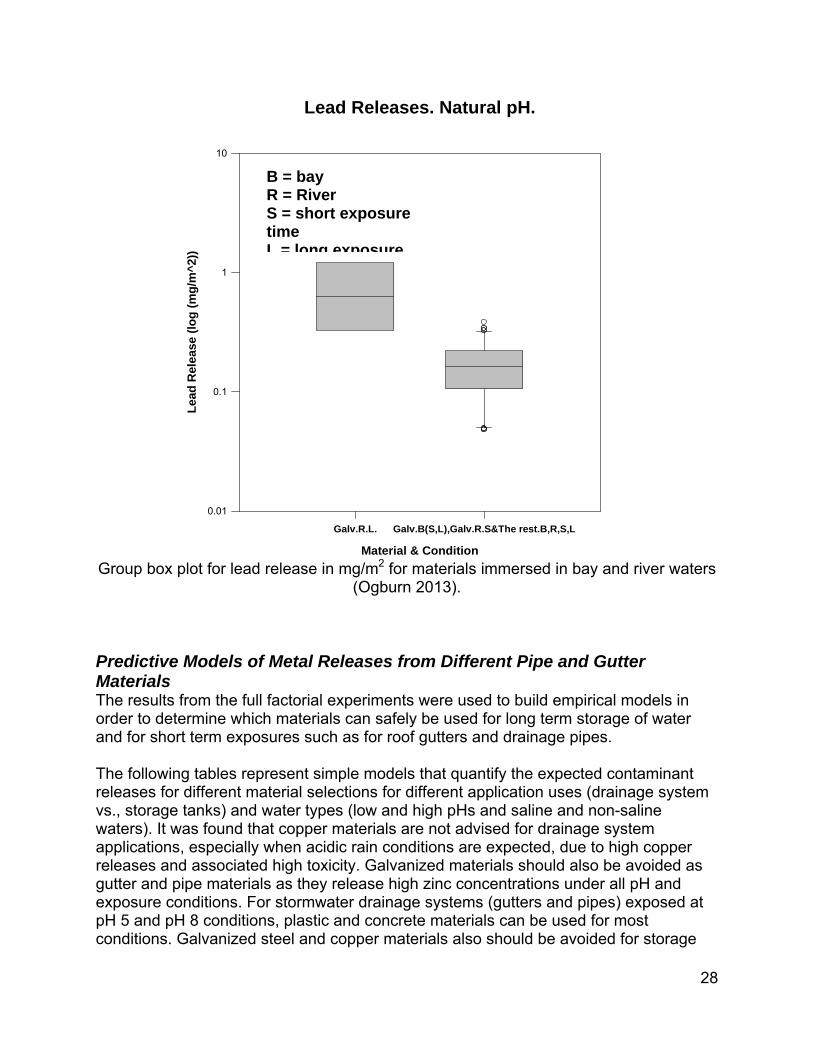
waters (Ogburn 2013). Long exposure periods increased lead releases in the samples with galvanized materials immersed into river water. However this tendency was not observed for galvanized steel materials immersed in bay water and can be explained by the metal releases being close to detection limit. Lead releases were combined in two groups.
S = short exposure time L = long exposure time
28
Lead Releases. Natural pH.
Material & Condition
Galv.R.L. Galv.B(S,L),Galv.R.S&The rest.B,R,S,L
Lea
d R
ele
ase
(lo
g (
mg
/m^
2))
0.01
0.1
1
10
Group box plot for lead release in mg/m2 for materials immersed in bay and river waters
(Ogburn 2013).
Predictive Models of Metal Releases from Different Pipe and Gutter Materials The results from the full factorial experiments were used to build empirical models in order to determine which materials can safely be used for long term storage of water and for short term exposures such as for roof gutters and drainage pipes. The following tables represent simple models that quantify the expected contaminant releases for different material selections for different application uses (drainage system vs., storage tanks) and water types (low and high pHs and saline and non-saline waters). It was found that copper materials are not advised for drainage system applications, especially when acidic rain conditions are expected, due to high copper releases and associated high toxicity. Galvanized materials should also be avoided as gutter and pipe materials as they release high zinc concentrations under all pH and exposure conditions. For stormwater drainage systems (gutters and pipes) exposed at pH 5 and pH 8 conditions, plastic and concrete materials can be used for most conditions. Galvanized steel and copper materials also should be avoided for storage
B = bay R = River S = short exposure time L = long exposure

29
tanks applications due to very high metal releases and toxicities. For stormwater storage applications, concrete, HDPE, and vinyl materials can be safely used due to their small, or non-detected, metal releases. Model based on 22 Factorial analyses. Steel pipe. Controlled pH tests (Ogburn 2013)
Constituent Galvanized Steel Pipe. Controlled pH Conditions Pb, mg/m2 Pb (mg/m2) = 0.0092*Time (hr); R2 = 59.2%; p-value for regression =0.00
Cu, mg/m2 Avg.= 0.60 - 1.28; Median = 0- 0.02; Min= 0; Max= 4.785; # of Pts above
DL: 3 Model based on 22 Factorial analyses. Steel materials. Controlled pH tests (Ogburn 2013)
Constituent Galvanized Steel Materials (Pipe and Gutter). Controlled pH Conditions
Zn, mg/m2
Log Zn (mg/m2) @pH5 = 2.138 +0.1904*logTime (hr);
R2 = 68.2%; p-value for regression = 0.001
Log Zn (mg/m2) @pH8 = 0.7236 +0.7643*logTime (hr);
R2 = 94.0%; p-value for regression = 0.000
Model groups based on 22 Factorial analyses. Steel pipe. Natural pH tests (Ogburn 2013)
Constituent
Galvanized Steel Pipe. Natural pH Conditions
Pb, mg/m2 S.B-: Avg.= 0.4 (COV = 0.22)
S.R.: Avg.= 0.1
(COV = 0.02) L.B-: Avg.= 0.1 (COV = 0.02)
L.R.: Avg.= 0.42 (COV = 0.79)
Cu, mg/m2 ND in bay and river waters
Zn, mg/m2 Log Zn (mg/m2) = 1.63 +0.51*logTime (hr); R2 = 81.2%; p-value for
regression = 0.00 Footnote: S. = short exposure time; L. = long exposure time; B- = bay; R. = river; ND = non-detects. Model based on 22 Factorial analyses. Copper gutter. Controlled pH tests (Ogburn 2013)
Constituent Copper Gutter. Controlled pH Conditions Pb, mg/m2 ND at pH 5 and 8 Cu, mg/m2 pH5: Avg.= 250 (COV = 0.66) pH 8: Avg.= 70.5 (COV = 0.96) Zn, mg/m2 pH5: Avg.= 3.2 (COV = 0.81) pH 8: Avg.= 0.22 (COV = 1.55) Footnote: ND = non-detects.

30
Model based on 22 Factorial analyses. Copper gutter. Natural pH tests (Ogburn 2013) Constituent Copper Gutter. Natural pH Conditions Pb, mg/m2 ND in bay and river waters
Cu, mg/m2
Bay Water: Log Cu (mg/m2) = 1.25 +0.59*logTime (hr);
R2 = 91.4%; p-value for regression = 0.002
River Water: Log Cu (mg/m2) = 0.72 +0.52*logTime (hr); R2 = 98.0%; p-value for
regression = 0.00
Zn, mg/m2 Avg.= 3.46 - 3.79; Median = 1.27-1.62; Min= -0.67**; Max= 29.51; # of Pts
above DL: 9 Footnote: ND = non-detects. ** the mg/m2 releases are compared to initial time zero conditions without the material in the test water. If the observed concentrations decreased with time (such as from precipitation on the material), the observed release rate was negative. Obviously, zero should be used in predictions instead of negative values. The models showed that copper materials had elevated copper releases in pH 5 waters (250 mg/m2) and in bay and river waters during short exposure times (180 and 840 mg/m2 respectively). Long term exposure periods of copper materials under both high and low salinity conditions also resulted in high copper releases (1490 and 240 mg/m2 respectively). Zinc concentrations released from galvanized steel materials were very high under both low and high pH conditions and during both short and long exposure times for controlled pH experiments (the average of 480 and 1860 mg/m2 for galvanized steel materials at pH 5 and pH8 conditions respectively during long exposure time). For natural pH tests, long exposure periods resulted in high zinc concentrations released from galvanized pipes for waters with both high and low salinities (2,230 mg/m2). Galvanized steel gutters immersed in bay and river waters had very high zinc releases during long term exposures (840 and 5,387 mg/m2 for bay and river waters respectively). Elevated lead releases from galvanized steel materials were observed for pH 5 and 8 waters during long exposure periods, and for bay waters during short exposure periods and river waters during long exposure periods for steel pipe and for steel gutter during natural pH tests. Chemical Speciation Modeling of Heavy Metals (Medusa Water Chemistry Modeling Environment) In stormwater, many heavy metals can sorb to inorganic and organic particulate matter that accumulate as bed sediments. Water chemistry, the suspended sediment and substrate sediment composition influence the behavior of heavy metals in natural waters. The sorption of heavy metals to particulates is affected by chemical identity, redox conditions, water pH, and complexation and precipitation chemistry (Clark and Pitt 2012). The forms of metal species present in the environment will affect toxicity and treatability of heavy metals. Comprehensive water chemistry modeling was conducted to predict the forms of the measured metals. Medusa software (Medusa, KTH, available at http://www.kemi.kth.se/medusa/) was used. Phase, Fraction, and Pourbaix diagrams show the predominant species of metals and their concentrations. For all chemical
31
components in Medusa files, only the concentrations at and above the detection limit were used. The diagrams and summary tables were made for zinc, copper, and lead. For Medusa input files, an assumption was made that equilibrium was reached during the static experiments. For the buffered test, total hardness and calcium hardness, chloride, and sulfate were measured after 3 months of exposure and were assumed to be representative of conditions during the whole time of the experiment. In the buckets with copper gutter at pH 5 and with aluminum gutter at pH 8, Ca hardness was less than the detection limit of 0.02 mg/L as CaCO3. For the un-buffered test, total hardness and calcium hardness were measured at time zero and after 3 months of exposure, therefore the hardness values after one day of exposure and was assumed to be equal to those measured at time zero. Since only one form of phosphorus species can be included into a Medusa file, H2PO4
- was used for solutions with pH 5 since at this pH, H2PO4
- is the predominant phosphorus species, and HPO42- for solutions with pH 8
since at pH 8, HPO42- is a predominant phosphorus species (Golubzov 1966). Other
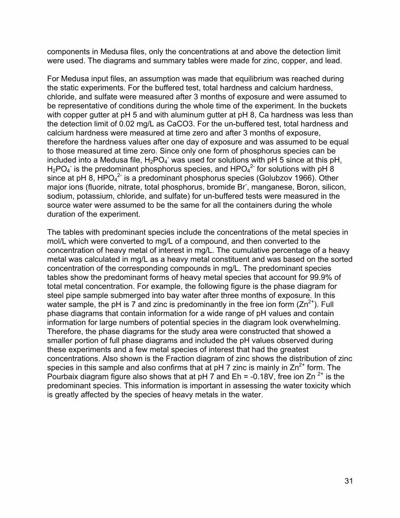
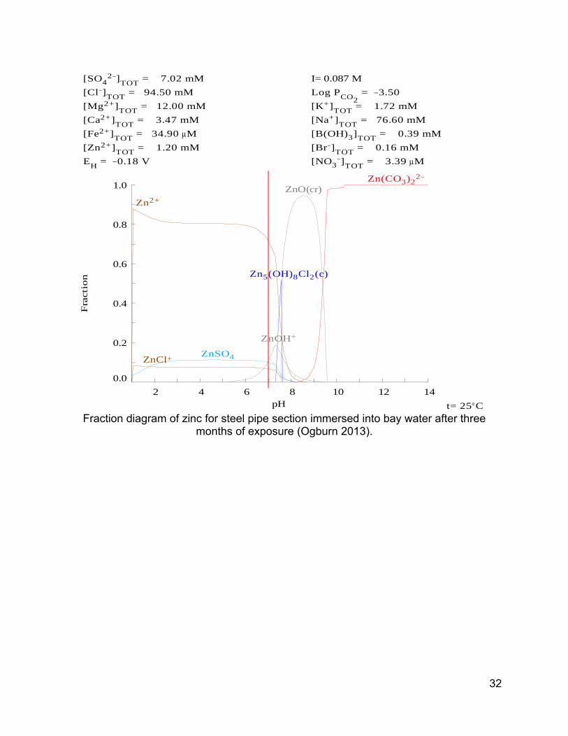
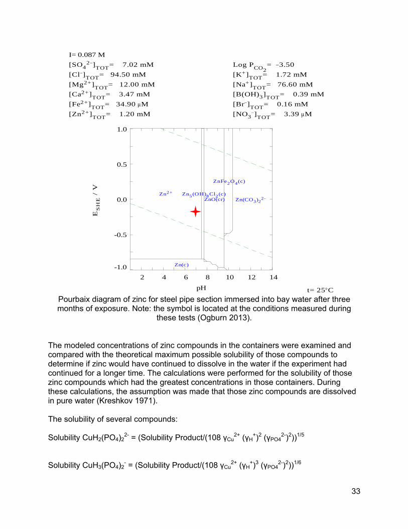
major ions (fluoride, nitrate, total phosphorus, bromide Br-, manganese, Boron, silicon, sodium, potassium, chloride, and sulfate) for un-buffered tests were measured in the source water were assumed to be the same for all the containers during the whole duration of the experiment. The tables with predominant species include the concentrations of the metal species in mol/L which were converted to mg/L of a compound, and then converted to the concentration of heavy metal of interest in mg/L. The cumulative percentage of a heavy metal was calculated in mg/L as a heavy metal constituent and was based on the sorted concentration of the corresponding compounds in mg/L. The predominant species tables show the predominant forms of heavy metal species that account for 99.9% of total metal concentration. For example, the following figure is the phase diagram for steel pipe sample submerged into bay water after three months of exposure. In this water sample, the pH is 7 and zinc is predominantly in the free ion form (Zn2+). Full phase diagrams that contain information for a wide range of pH values and contain information for large numbers of potential species in the diagram look overwhelming. Therefore, the phase diagrams for the study area were constructed that showed a smaller portion of full phase diagrams and included the pH values observed during these experiments and a few metal species of interest that had the greatest concentrations. Also shown is the Fraction diagram of zinc shows the distribution of zinc species in this sample and also confirms that at pH 7 zinc is mainly in Zn2+ form. The Pourbaix diagram figure also shows that at pH 7 and Eh = -0.18V, free ion Zn 2+ is the predominant species. This information is important in assessing the water toxicity which is greatly affected by the species of heavy metals in the water.
32
Fraction diagram of zinc for steel pipe section immersed into bay water after three
months of exposure (Ogburn 2013).
2 4 6 8 10 12 14
0.0
0.2
0.4
0.6
0.8
1.0
Fra
ctio
n
pH
Zn2+
Zn(CO3)22
ZnCl+
ZnOH+
ZnSO4
Zn5(OH)8Cl2(c)
ZnO(cr)
EH
= 0.18 V
[Zn2+]TOT = 1.20 mM
[Fe2+]TOT
= 34.90 M[Ca2+]
TOT = 3.47 mM
[Mg2+]TOT = 12.00 mM
[Cl]TOT
= 94.50 mM
[SO42]
TOT = 7.02 mM
[NO3]
TOT = 3.39 M
[Br]TOT = 0.16 mM
[B(OH)3]TOT
= 0.39 mM
[Na+]TOT
= 76.60 mM
[K+]TOT = 1.72 mM
Log PCO2
= 3.50
I= 0.087 M
t= 25C
33
Pourbaix diagram of zinc for steel pipe section immersed into bay water after three months of exposure. Note: the symbol is located at the conditions measured during
these tests (Ogburn 2013). The modeled concentrations of zinc compounds in the containers were examined and compared with the theoretical maximum possible solubility of those compounds to determine if zinc would have continued to dissolve in the water if the experiment had continued for a longer time. The calculations were performed for the solubility of those zinc compounds which had the greatest concentrations in those containers. During these calculations, the assumption was made that those zinc compounds are dissolved in pure water (Kreshkov 1971). The solubility of several compounds: Solubility CuH2(PO4)2
2- = (Solubility Product/(108 γCu2+ (γH
+)2 (γPO42-)2))1/5
Solubility CuH3(PO4)2
- = (Solubility Product/(108 γCu2+ (γH
+)3 (γPO42-)2))1/6
2 4 6 8 10 12 14
-1.0
-0.5
0.0
0.5
1.0
ES
HE
/ V
pH
Zn2+
Zn(CO3)22
Zn(c)
Zn5(OH)8Cl2(c)ZnO(cr)
ZnFe2O4(c)
[Zn2+]TOT
= 1.20 mM
[Fe2+]TOT= 34.90 M[Ca2+]TOT= 3.47 mM
[Mg2+]TOT
= 12.00 mM
[Cl]TOT= 94.50 mM
[SO42]TOT= 7.02 mM
[NO3]
TOT= 3.39 M
[Br]TOT= 0.16 mM
[B(OH)3]TOT= 0.39 mM
[Na+]TOT
= 76.60 mM
[K+]TOT= 1.72 mM
Log PCO2= 3.50
I= 0.087 M
t= 25C

34
Solubility Zn5(OH)6(CO3)2 = (Solubility Product/(0.48 (γZn
2+)5 (γOH-)6 (γCO3
2-)2))1/13 The solubility of compounds with the KtAn formula (Kreshkov 1971): Solubility KtAn- = (Solubility ProductKtAn/(γKt γAn))
1/2 Where, Kt = cation An = anion γ = activity coefficient of cation or anion. The solubility of compounds with the KtAn2 formula (Kreshkov 1971): Solubility KtAn2 = (Solubility ProductKtAn2/(4 γKt (γAn)
2))1/3 The solubility of compounds with the Kt2An formula (Kreshkov 1971): Solubility Kt2An = (Solubility ProductKt2An/(4 (γKt)
2 γAn))1/3
The solubility of compounds with the Kt3An2formula (Kreshkov 1971): Solubility Kt3An2 = (Solubility ProductKt3An2/(108 (γKt)
3 (γAn)2))1/5
The solubility formulas of other compounds can be found in Kreshkov 1971. The following table shows solubility products for some reactions. The rest of the solubility products were taken from Medusa. Medusa is available from http://www.kemi.kth.se/medusa/. Solubility products
Equation Solubility Product, Ksp Reference Zn(OH)2 Zn2+ + 2OH- 1.4 *10-17 (Lurie 1989) ZnCO3 Zn2+ + CO3
2- 1.45 *10-11 (Lurie 1989) Medusa results showed that during the buffered pH tests, Zn3(PO4)2:4H2O(c) likely precipitated in the containers with galvanized steel pipe immersed in pH 5 and pH 8 waters after three months of exposure. The solubility product for Zn3(PO4)2:4H2O(c) is very small (Ksp = 9.1 *10-33 (Lurie 1989)) and Zn3(PO4)2:4H2O(c) easily precipitates. In pure water, not taking into consideration hydrolysis of phosphoric acid and complex formation, the amount of Zn3(PO4)2:4H2O that can dissolve in water is 5.6E-07mol/L (0.11 mg/L as Zn), however due to hydrolysis and complexation the amount of dissolved Zn3(PO4)2:4H2O was greater that the theoretical value and reached 3.37E-05 mol/L (6.62 mg/L as Zn) in the container with galvanized steel pipe immersed into pH 5 water. Golubzov (1966) pointed out that hydrolysis increases the solubility of insoluble salts in the solution.

35
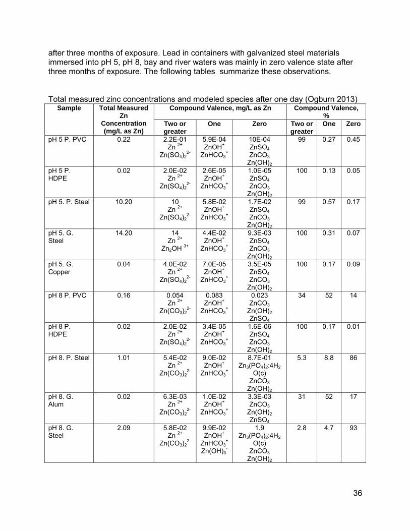
The following tables show total measured metal concentrations and modeled metal species at time zero (base water alone), after one day of exposure and after three months of exposure. The total percent of compound valence doesn’t always add up to 100 due to the rounding. At time zero (water without pipes and gutters), zinc and zinc compounds were predominantly in valence two state in the containers with pH 5 water, and were mostly in valence one state in the containers with pH 8 water. At time zero, copper and copper compounds in the buckets with pH 5 and 8 waters were mainly in valence two state. After one day of exposure, zinc and zinc compounds were predominantly in valence two state in the samples with steel, copper, and plastic materials immersed in pH 5 water, and mainly in zero and one valence states in the samples with steel, copper, aluminum, and plastic materials immersed in pH 8 water. After one day of exposure, copper and copper compounds in containers with copper materials immersed into pH 5 water were approximately equally distributed between valence states of two, one, and zero, however for the buffered pH 8 waters, copper compounds in containers with copper gutters were predominantly in valence two state which can be explained by the formation of copper complexes with phosphate and other ions. Copper was generally in valence zero state in the samples with copper materials immersed in bay and river waters. Sandberg, et al. (2006) examined corrosion-induced copper runoff from copper sheet, naturally patinated copper and pre-patinated copper in a chloride-rich marine environment during one year. The bioavailable concentration (the portion that is available for uptake by an organism) of released copper comprised a small fraction (14–54%) of the total copper concentration due to complexation towards organic matter in impinging seawater aerosols (Sandberg, et. al., 2006). The authors concluded that released copper is complexed with other ligands which reduce the bioavailability. Factors that influence the bioavailability of copper include alkalinity, hardness, pH and dissolved organic matter. Seawater contains organic matter that is primarily of biotic origin, and a significant portion of copper is most likely complexed with these ligands, which leads to reduction of the bioavailability (Sandberg, et. al., 2006). In this research, the results from Medusa modeling showed that copper released in the containers with copper gutter materials immersed into bay water was almost all in valence zero state. For containers with galvanized steel materials immersed into buffered pH 8 and bay waters, lead was mainly in valence zero after one day of exposure. After three months of exposure, zinc and zinc compounds in the containers with galvanized steel, copper, aluminum, and plastic materials immersed into buffered pH 5 water were mainly in valence two state after; for galvanized steel, copper, aluminum, concrete, and plastic materials immersed into buffered pH 8, bay, and river waters, zinc was in one or zero valence states. For containers with copper materials immersed into pH 5 water, the valence state of copper and cooper compounds was approximately equally distributed between two, one, and zero and for copper materials submerged into buffered pH 8, bay, and river waters copper was predominantly in zero valence state
36
after three months of exposure. Lead in containers with galvanized steel materials immersed into pH 5, pH 8, bay and river waters was mainly in zero valence state after three months of exposure. The following tables summarize these observations. Total measured zinc concentrations and modeled species after one day (Ogburn 2013)
Sample Total Measured Zn
Concentration (mg/L as Zn)
Compound Valence, mg/L as Zn Compound Valence, %
Two or greater
One Zero Two or greater
One Zero
pH 5 P. PVC 0.22 2.2E-01 Zn 2+
Zn(SO4)22-
5.9E-04 ZnOH+
ZnHCO3+
10E-04 ZnSO4 ZnCO3
Zn(OH)2
99 0.27
0.45
pH 5 P. HDPE
0.02
2.0E-02 Zn 2+
Zn(SO4)22-
2.6E-05 ZnOH+
ZnHCO3+
1.0E-05 ZnSO4 ZnCO3
Zn(OH)2
100 0.13
0.05
pH 5. P. Steel 10.20
10 Zn 2+
Zn(SO4)22-
5.8E-02 ZnOH+
ZnHCO3+
1.7E-02 ZnSO4 ZnCO3
Zn(OH)2
99 0.57
0.17
pH 5. G. Steel
14.20
14 Zn 2+
Zn2OH 3+
4.4E-02 ZnOH+
ZnHCO3+
9.3E-03 ZnSO4 ZnCO3
Zn(OH)2
100 0.31
0.07
pH 5. G. Copper
0.04
4.0E-02 Zn 2+
Zn(SO4)22-
7.0E-05 ZnOH+
ZnHCO3+
3.5E-05 ZnSO4 ZnCO3
Zn(OH)2
100 0.17
0.09
pH 8 P. PVC 0.16
0.054 Zn 2+
Zn(CO3)22-
0.083 ZnOH+
ZnHCO3+
0.023 ZnCO3
Zn(OH)2 ZnSO4
34
52
14
pH 8 P. HDPE
0.02
2.0E-02 Zn 2+
Zn(SO4)22-
3.4E-05 ZnOH+
ZnHCO3+
1.6E-06 ZnSO4 ZnCO3
Zn(OH)2
100
0.17
0.01
pH 8. P. Steel 1.01
5.4E-02 Zn 2+
Zn(CO3)22-
9.0E-02 ZnOH+
ZnHCO3+
8.7E-01 Zn3(PO4)2:4H2
O(c) ZnCO3
Zn(OH)2
5.3 8.8
86
pH 8. G. Alum
0.02
6.3E-03 Zn 2+
Zn(CO3)22-
1.0E-02 ZnOH+
ZnHCO3+
3.3E-03 ZnCO3
Zn(OH)2 ZnSO4
31 52
17
pH 8. G. Steel
2.09
5.8E-02 Zn 2+
Zn(CO3)22-
9.9E-02 ZnOH+
ZnHCO3+
Zn(OH)3-
1.9 Zn3(PO4)2:4H2
O(c) ZnCO3
Zn(OH)2
2.8 4.7
93

37
Total measured zinc concentrations and modeled species after one day (Ogburn 2013), continued pH 8. G. Copper
0.02 5.9E-03 Zn 2+
Zn(CO3)22-
1.0E-02 ZnOH+
ZnHCO3+
3.8E-03 ZnCO3
Zn(OH)2 ZnSO4
30 52 19
Bay P. Steel 8.4 0.2 Zn 2+
Zn(CO3)22-
Zn(SO4)22-
0.42 ZnOH+ ZnCl+
ZnHCO3+
7.8 Zn5(OH)6(CO3)2
(c) ZnFe2O4(c)
ZnCO3
2.3 5.0 93
Bay G. Steel 4.8 0.20 Zn 2+
Zn(CO3)22-
Zn(SO4)22-
0.42 ZnOH+ ZnCl+
ZnHCO3+
4.2 Zn5(OH)6(CO3)2
(c) ZnFe2O4(c)
ZnCO3
4.1 8.7 87
Bay G. Copper
0.05 1.4E-02 Zn 2+
Zn(CO3)22-
Zn(SO4)22-
2.6E-02 ZnOH+ ZnCl+
ZnHCO3+
1.0E-02 ZnCO3
Zn(OH)2 ZnSO4
28 52 20
River P. Steel 6.1 0.25 Zn(CO3)2
2- Zn 2+
Zn(SO4)22-
0.17 ZnOH+
ZnHCO3+
Zn(OH)3-
5.6 Zn5(OH)6(CO3)2
(c) ZnCO3
ZnFe2O4(c)
4.2 2.8 93
River G. Steel
1.20 0.19 Zn(CO3)2
2- Zn 2+
Zn(SO4)22-
0.20 ZnOH+
ZnHCO3+
Zn(OH)3-
0.82 Zn5(OH)6(CO3)2
ZnCO3 ZnFe2O4(c)
16 16 68
River G. Copper
0.02 3.2E-03 Zn 2+
Zn(CO3)22-
Zn(SO4)22-
1.1E-02 ZnOH+
ZnHCO3+
ZnCl+
5.4E-03 ZnCO3
Zn(OH)2 ZnSO4
16 57 27

38
Total measured copper concentrations and modeled species after one day (Ogburn 2013)
Sample Total Measured Cu
Concentration (mg/L as Cu)
Compound Valence, mg/L as Cu Compound Valence, %
Two or greater
One Zero Two or greater
One Zero
pH 5 P. PVC 0.08 3.7E-02 CuH2(PO4)2
2
- Cu 2+
CuH3(PO4)22
-
2.1E-02 CuH2PO4
+ CuH3(PO4
)2-
Cu+
2.3E-02 CuHPO4 CuH2PO4
Cu(H2PO4)2
46
26
28
pH 5 G. Copper
6.82
2.5 CuH2(PO4)2
2
- Cu 2+
CuH3(PO4)22
-
2.5 CuH2PO4
+ CuH3(PO4
)2-
Cu+
1.8 CuHPO4
Cu(H2PO4)2 CuH2PO4
37 36
27
pH 8 P. PVC 0.08
7.8E-02 CuH2(PO4)2
2
- CuH3(PO4)2
2
- Cu 2+
1.2E-04 Cu(OH)2
- Cu+
CuOH+
1.7E-03 CuHPO4 CuCO3
Cu(OH)2
98 0.15
2.1
pH 8 G. Copper
0.29
2.8E-01 CuH2(PO4)2
2
- Cu 2+
CuH3(PO4)22
-
2.5E-04 Cu(OH)2
- CuOH+
Cu+
6.5E-03 CuHPO4 CuCO3
Cu(OH)2
98 8.8E-02
2.2
Bay G. Copper
2.11 1.1E-04 CuCl3
2- Cu2Cl4
2- Cu 2+
3.2E-03 CuCl2
- Cu+
Cu(OH)2-
2.1 Cu(c)
CuFeO2(c) CuSO4
5.0E-03
0.15 100
River G. Copper
0.60 5.5E-09 CuCl3
2- Cu 2+
Cu(CO3)22-
1.9E-05 CuCl2
- Cu(OH)2
- Cu+
0.6 Cu(c)
CuFeO2(c) CuCO3
9.2E-07
3.2E-03
100

39
Total measured lead concentrations and modeled species after one day (Ogburn 2013) Sample Total Measured
Pb Concentration (mg/L as Pb)
Compound Valence, mg/L as Pb Compound Valence, % Two or greater
One Zero Two or greater
One Zero
pH 8 G. Steel 0.008
5.9E-05 Pb(CO3)2
2- Pb 2+
1.8E-05 PbOH+
PbHCO3+
8.0E-03 Pb3(PO4)2(
c) PbCO3
PbHPO4
0.73 0.22
99
Bay P. Steel 0.012 1.1E-03 Pb(CO3)2
2- Pb 2+
Pb(SO4)22-
4.6E-04 PbOH+ PbCl+
PbHCO3+
1.1E-02 PbCO3 PbSO4
Pb(OH)2
9.3 3.8 87
Bay G. Steel 0.005 4.7E-04 Pb(CO3)2
2- Pb 2+
Pb(SO4)22-
1.9E-04 PbOH+ PbCl+
PbHCO3+
4.4E-03 PbCO3 PbSO4
Pb(OH)2
9.3 3.8 87
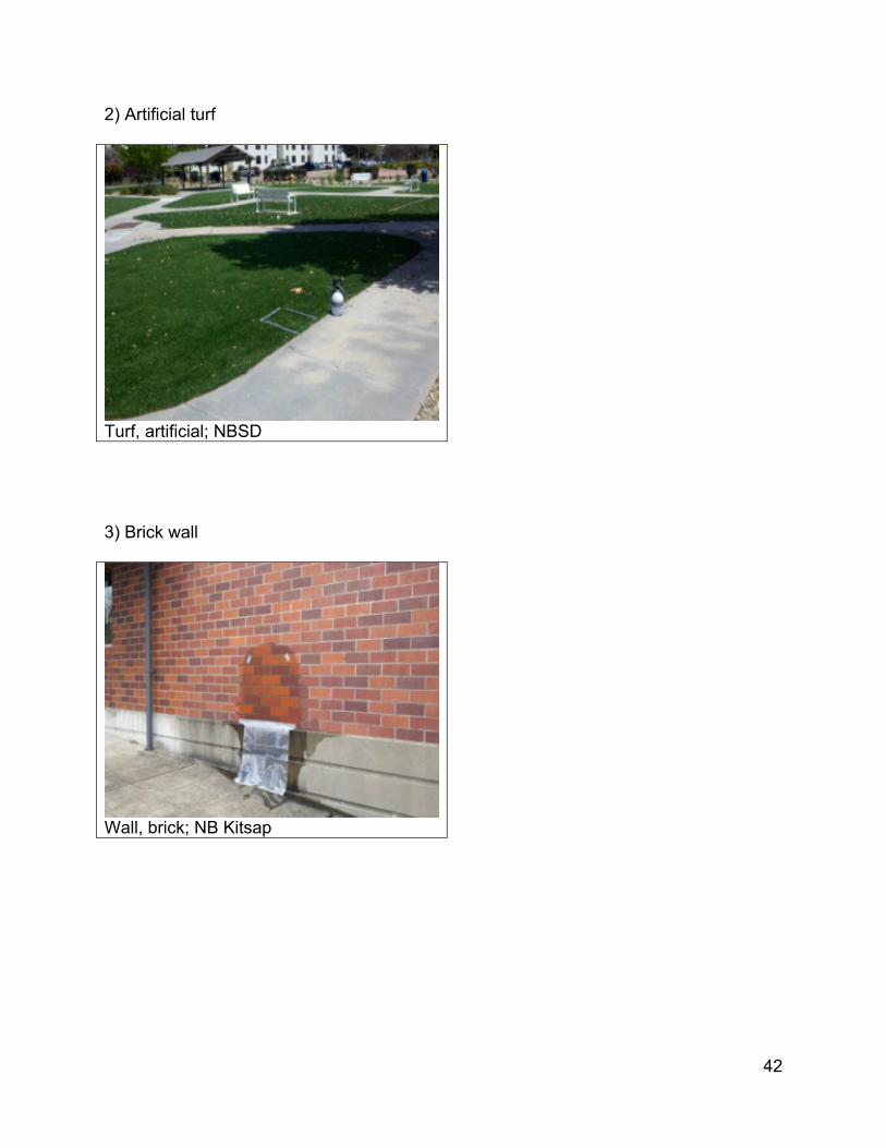
Washdown Tests of Exposed Materials at Naval Facilities SPAWARSYSCEN-PACIFIC Navy personnel conducted a series of material washoff tests as part of this research project. The following pictures show the how these tests were conducted for several different types of materials. Generally, 2 to 4 L of DI water was gently sprayed over a known area (about 2 ft2) with the wash water collected in a plastic tray. Each test lasted about 15 to 30 minutes. The wash water was then chemically analyzed for a suite of heavy metals. This section includes photographs of many of the materials tested, and the data grouped by material type. The 79 materials were sorted into the following 16 categories for these data summaries: aluminum ramp, artificial turf, brick wall, concrete, galvanized metal (bare), galvanized metal (painted), galvanized metal (coated), barge hull, metal (bare), metal (painted), plaster, roof, rubber, wood (bare), wood (painted), and wood (treated). Some of these categories have only a single sample, while others have many. The data are presented by metal. The first table shows the available data for each category, along with simple summary statistics. These data were then evaluated in SigmaPlot (version 15) using the non-parametric Kruskal-Wallis one way analysis of variance on ranks to determine if at least one group is significantly different from any of the others (this test only examines single groups). Simultaneously, grouped box and whisker plots were prepared in SigmaPlot for these groups. These results were then used to group the groups into a fewer number of combined groups indicating materials that had low washoff concentrations, high concentrations, and the other categories. Box and whisker plots and Kruskal-Wallis analyses were also used to evaluate these

40
categories. These data summaries, plots, and analyses were made for both the concentration and the unit area loading washoff data.
Washdown setups showing sprayer, plastic sheet below target area and plastic tray to capture washdown water (barge hull).
Washdown sampling for untreated wood.
Washdown sampling for engine block.

41
Washdown sampling for tires.
Washdown sampling of galvanized stair steps.
1) Aluminum ramp
Walkway, aluminum; Everett
42
2) Artificial turf
Turf, artificial; NBSD 3) Brick wall
Wall, brick; NB Kitsap

43
4) Concrete
Concrete wall; SSC-PAC Concrete barrier, uncoated; Saint Julian
5) Galvanized, bare
Galvanized shed, sides; NBK Bangor Galvanized rail; SUBASE

44
Galvanized fence; SUBASE
Galvanized scaffold stack, laydown area; SUBASE
Causeway, portion with zinc anode; Little Creek
Pallet, galvanized (folded); Saint Julian
Utility pole, galvanized; NB Kitsap Sheath, over concrete barrier edge;
Everett

45
Stairs, galvanized; Everett Scaffold parts, galvanized; Pt. Loma
Subase
Grate 1, stormwater drain; NBSD Grate 2, stormwater drain; NBSD

46
6) Galvanized, painted
Galvanize siding, painted, chipped; NBK Bangor Metal panel, painted galvanized, building
side; Saint Julian
Fence, painted galvanized; NB Kitsap

47
7) Galvanized, coated
Coated galvanized fence; SSC=PAC 8) Barge hull
Barge hull; Little Creek Barge hull; Little Creek
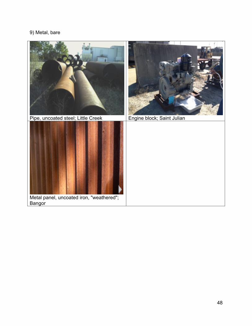
48
9) Metal, bare
Pipe, uncoated steel; Little Creek Engine block; Saint Julian
Metal panel, uncoated iron, "weathered"; Bangor
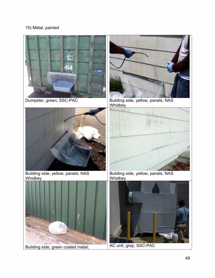
49
10) Metal, painted
Dumpster, green; SSC-PAC Building side, yellow, panels; NAS Whidbey
Building side, yellow, panels; NAS Whidbey
Building side, yellow, panels; NAS Whidbey
Building side, green coated metal;
AC unit, gray; SSC-PAC

50
NAVSTA Everett
Electrical vault, green; SSC-PAC Keel blocks, metal painted; Little Creek
Causeway, gray painted side; Little Creek Metal panel, light yellow (temp. buildings); NB Kitsap
Metal panel, painted light yellow; Bangor Metal, painted, brick red; Bangor

51
Fire hydrant, red; Everett
Guard rail, painted yellow; Pt. Loma Subase
Water riser, potable, blue (w/brass part); Pt. Loma Subase
Water riser, potable, blue; Pt. Loma Subase
Pipe supports, metal, painted brown; Pt. Loma Subase
Dumpster (blue), cardboard recycle; SSC-PAC

52
Dumpster (blue), cardboard recycle w/guano, heron; SSC-PAC
11) Plaster siding
Plaster wall, painted white; SSC-PAC

53
12) Roof
Shed roof, green coated metal; NAVSTA Everett
Shingles, asphalt; Bangor
Roof, (via gutter); Bangor

54
13) Rubber
Cable, black, 4” diameter; SUBASE Cable, black, 4” diameter; SUBASE
Tires, rubber; Saint Julian Bumpers, large, black; Everett
Cables, electrical 3 in. diameter; Pt. Loma Subase
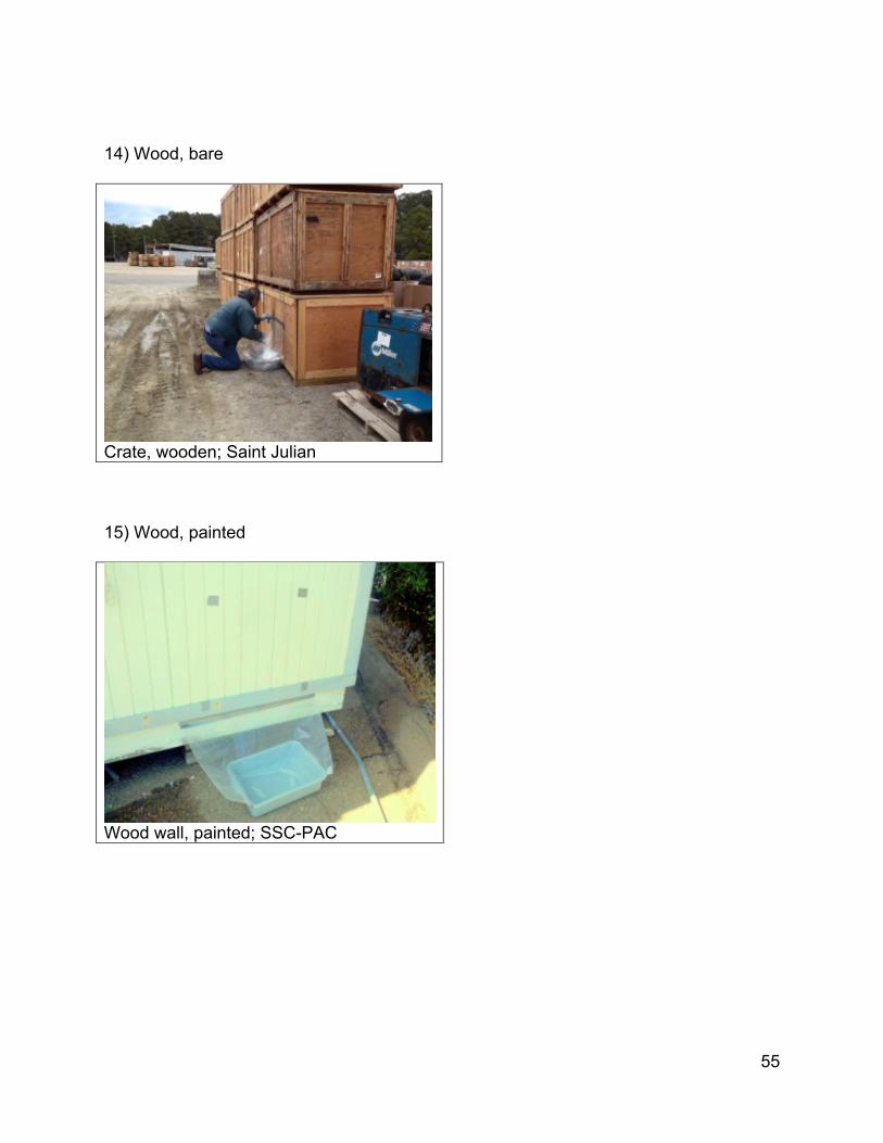
55
14) Wood, bare
Crate, wooden; Saint Julian 15) Wood, painted
Wood wall, painted; SSC-PAC

56
16) Wood, treated
Wood, treated, green; NBK Bangor
Treated wood, green painted; SUBASE
Wood, treated (copper azole); Little Creek Treated wood label; Little Creek

57
Aluminum Aluminum Washdown Concentrations (µg/L)
Grouped Category:
high other other other other high other other low other low high other
Sample Category:
Al ramp
artificial turf
brick wall
concrete galv bare
galv painted
barge hull
metal bare
metal painted
roof rubber wood bare
wood treated
702 141 119 204 103 1,777 150 20 185 446 52 586 197
584 4 211 22 11 85
115 26 8 62
46 298 48
2 1,364
214 46
60 51
69 6
1,153 597
14
5
2
4
Grouped Category:
high other other other other high other other low other low high other
Sample Category:
Al ramp
artificial turf
brick wall
concrete galv bare
galv painted
barge hull
metal bare
metal painted
roof rubber wood bare
wood treated
number 1 1 1 1 9 2 1 4 13 2 3 1 1
min 2 4 20 2 11 52
max 1,153 1,777 298 1,364 446 85
average 261 890 139 181 229 66
median 702 141 119 204 103 890 150 118 22 229 62 586 197
st dev 377 1,253 138 391 308 17
COV 1.4 1.4 1.0 2.2 1.3 0.3

58
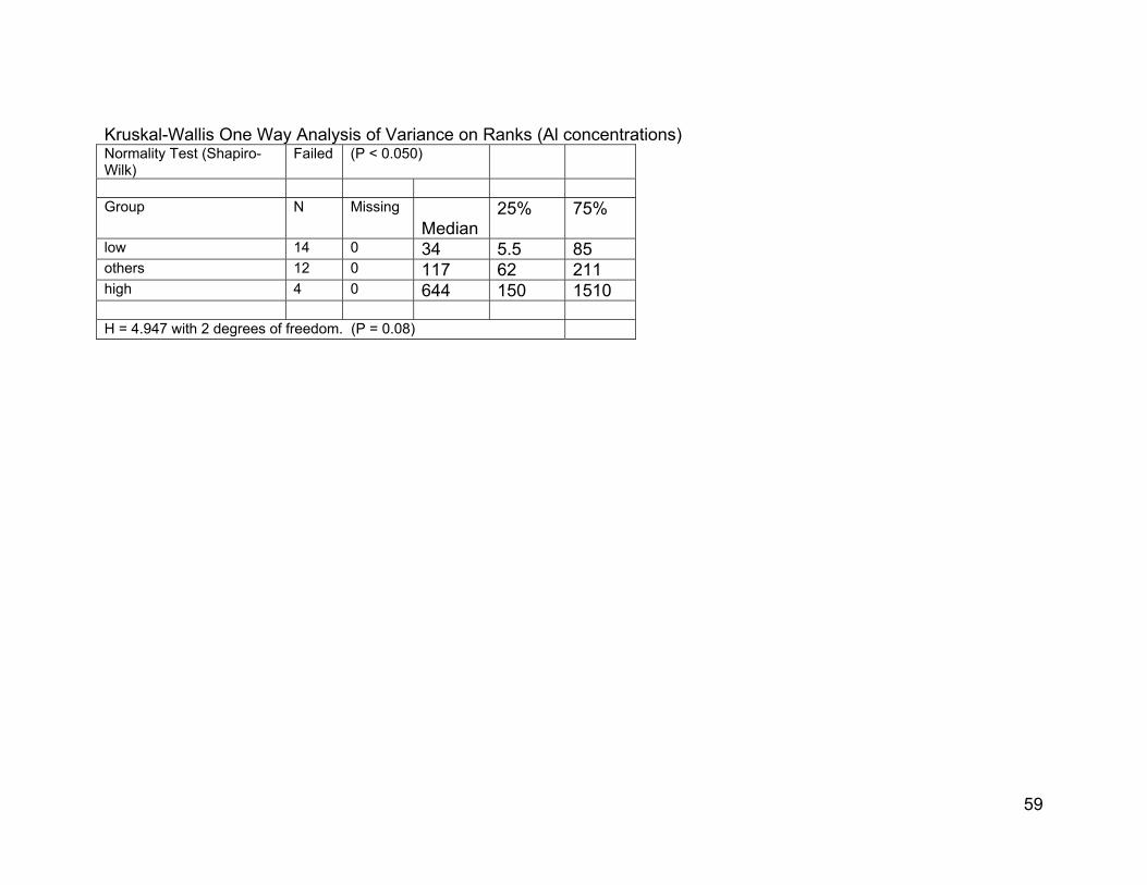
59
Kruskal-Wallis One Way Analysis of Variance on Ranks (Al concentrations) Normality Test (Shapiro-Wilk)
Failed (P < 0.050)
Group N Missing
Median 25% 75%
low 14 0 34 5.5 85 others 12 0 117 62 211 high 4 0 644 150 1510 H = 4.947 with 2 degrees of freedom. (P = 0.08)

60

61
Summary Statistics for Aluminum Concentration Grouped Categories Grouped category:
low all others high
Sample Category in Groups:
metal painted rubber
artificial turf brick wall concrete galv bare barge hull metal bare roof wood treated
Al ramp galv painted
number 14 12 4 min 1.8 2.4 4.0 max 1,360 1,150 1,780 average 172 234 770 median 34 117 644 st dev 380 326 739 COV 2.2 1.4 1.0

62
Aluminum Washdown Mass (µg/ft2)
Grouped Category:
high other other other other high other low low other low high other
Sample Category:
Al ramp
artificial turf
brick wall
concrete galv bare
galv painted
barge hull
metal bare
metal painted
roof rubber wood bare
wood treated
1,418 133 113 257 391 1,378 142 26 4 317 49 555 187
552 4 200 447 10 137
109 29 20 58
138 357 8
2 116
540 3,442
169 43
140 259
1,091 5
452
35
5
2
Grouped Category:
high other other other other high other low low other low high other
Sample Category:
Al ramp
artificial turf
brick wall
concrete galv bare
galv painted
barge hull
metal bare
metal painted
roof rubber wood bare
wood treated
number 1 1 1 1 9 2 1 4 13 2 3 1 1
min 2 4 26 2 10 49
max 1,091 1,378 357 3,442 317 137
average 348 691 153 372 164 81
median 1,418 133 113 257 169 691 142 114 35 164 58 555 187
st dev 341 972 158 937 217 48
COV 1.0 1.4 1.0 2.5 1.3 0.6

63
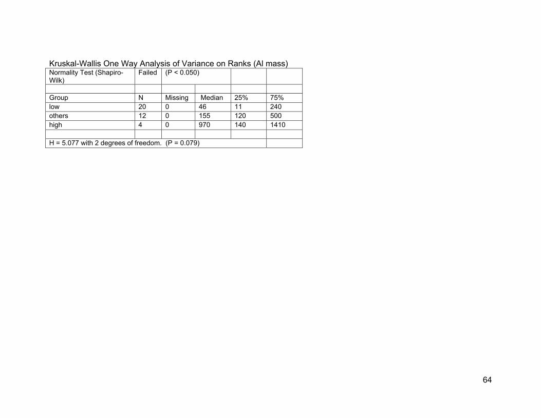
64
Kruskal-Wallis One Way Analysis of Variance on Ranks (Al mass) Normality Test (Shapiro-Wilk)
Failed (P < 0.050)
Group N Missing Median 25% 75% low 20 0 46 11 240 others 12 0 155 120 500 high 4 0 970 140 1410 H = 5.077 with 2 degrees of freedom. (P = 0.079)

65

66
Summary Statistics for Aluminum Mass Grouped Categories Grouped Category:
low others high
Sample Categories in Groups:
metal bare metal painted rubber
artificial turf brick wall concrete galv bare barge hull roof wood treated
Al ramp galv painted wood bare
number 20 12 4 min 1.7 2.1 3.8 max 3,440 1,090 1,420 average 285 303 839 median 46 155 966 st dev 758 304 684 COV 2.7 1.0 0.8

67
Cadmium Cadmium Washdown Concentrations (µg/L)
Grouped Category:
other other other other other other other other other other other other other
Sample Category:
Al ramp
artificial turf
brick wall
concrete galv bare
galv painted
barge hull
metal bare
metal painted
roof rubber wood bare
wood treated
0.1 0.2 0.1 0.5 0.1 2.3 0.9 0.1 0.0 0.2 0.1 0.6 0.4
1.1 0.2 163 131 0.1 0.4
0.1 0.1 0.2 0.3
1.7 0.0 0.1
0.3 0.2
1.4 0.9
0.2 0.1
0.2 0.1
0.1 0.1
0.9
0.2
0.1
0.1
Sample Category:
Al ramp
artifical turf
brick wall
concrete galv bare
galv painted
barge hull
metal bare
metal painted
roof rubber wood bare
wood treated
number 1 1 1 1 9 2 1 4 13 2 3 1 1
min 0.1 0.2 0.0 0.0 0.1 0.1
max 1.7 2.3 163.0 131.3 0.2 0.4
average 0.6 1.2 40.8 10.3 0.1 0.3
median 0.1 0.2 0.1 0.5 0.2 1.2 0.9 0.1 0.1 0.1 0.3 0.6 0.4
st dev 0.6 1.5 81.5 36.4 0.1 0.1
COV 1.1 1.2 2.0 3.5 0.6 0.6

68
One bare metal and one painted metal sample had very high (>100 ug/L) Cd concentrations; all others were very low (<1 µg/L). No significant groupings of data.

69
Summary Statistics for Cadmium Concentration Grouped Categories All combined number 40 min 0.05 max 160 average 7.7 median 0.18 st dev 33 COV 4.2
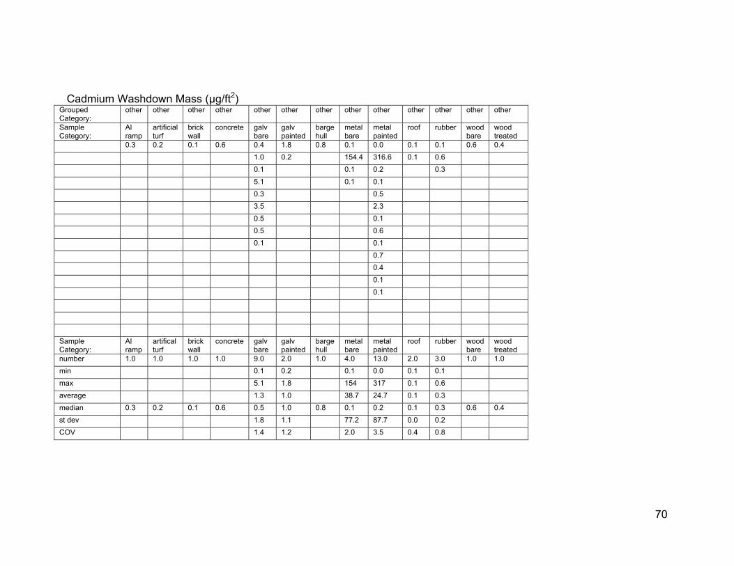
70
Cadmium Washdown Mass (µg/ft2)
Grouped Category:
other other other other other other other other other other other other other
Sample Category:
Al ramp
artificial turf
brick wall
concrete galv bare
galv painted
barge hull
metal bare
metal painted
roof rubber wood bare
wood treated
0.3 0.2 0.1 0.6 0.4 1.8 0.8 0.1 0.0 0.1 0.1 0.6 0.4
1.0 0.2 154.4 316.6 0.1 0.6
0.1 0.1 0.2 0.3
5.1 0.1 0.1
0.3 0.5
3.5 2.3
0.5 0.1
0.5 0.6
0.1 0.1
0.7
0.4
0.1
0.1
Sample Category:
Al ramp
artifical turf
brick wall
concrete galv bare
galv painted
barge hull
metal bare
metal painted
roof rubber wood bare
wood treated
number 1.0 1.0 1.0 1.0 9.0 2.0 1.0 4.0 13.0 2.0 3.0 1.0 1.0
min 0.1 0.2 0.1 0.0 0.1 0.1
max 5.1 1.8 154 317 0.1 0.6
average 1.3 1.0 38.7 24.7 0.1 0.3
median 0.3 0.2 0.1 0.6 0.5 1.0 0.8 0.1 0.2 0.1 0.3 0.6 0.4
st dev 1.8 1.1 77.2 87.7 0.0 0.2
COV 1.4 1.2 2.0 3.5 0.4 0.8
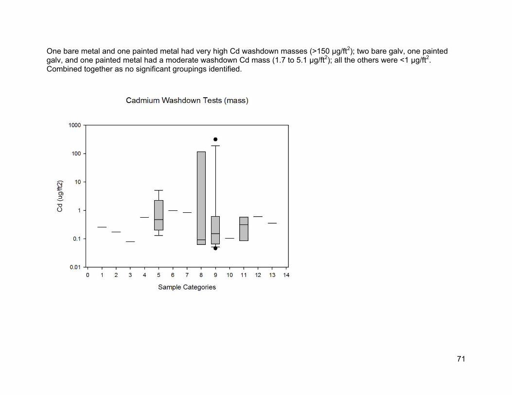
71
One bare metal and one painted metal had very high Cd washdown masses (>150 µg/ft2); two bare galv, one painted galv, and one painted metal had a moderate washdown Cd mass (1.7 to 5.1 µg/ft2); all the others were <1 µg/ft2. Combined together as no significant groupings identified.

72
Summary Statistics for Cadmium Mass Grouped Categories All Combined number 40 min 0.05 max 316 average 12.3 median 0.29 st dev 55 COV 4.5

73
Copper Copper Washdown Concentrations (µg/L) Grouped Category:
low other low low other other other high other other low low other other other high
Sample Category:
Al ramp
artificial turf
brick wall
concrete galv bare
galv painted
galv coated
barge hull
metal bare
metal painted
plaster roof rubber wood bare
wood painted
wood treated
4 93 2 81 1 6 15 30,334 57 42 2 5 1 17 6 5,417
1 2 13 5 12 2 5 20 179
2 29 2 1 4 1 1 6 27
2 7 3 51 1 34
1 2 5 10 1 11
1 1 4 3
3 3 98
6 52 167
4 12 3
27 3
174 3
22 2
1
2
24
3
1
19
0
11
2
0
0
3
3
3
Grouped Category:
low other low low other other other high other other low low other other other high
Sample Al artificial brick concrete galv galv galv barge metal metal plaster roof rubber wood wood wood

74
Category: ramp turf wall bare painted coated hull bare painted bare painted treated
number 1 1 1 9 12 3 1 1 5 26 3 5 6 1 1 3
min 1 1 2 1 0 1 1 1 27
max 81 174 13 57 167 2 5 34 5,417
average 11 28 7 14 18 2 3 13 1,874
median 4 93 2 2 9 6 15 30,334 5 3 2 1 9 17 6 179
st dev 26 49 5 24 37 0 2 13 3,069
COV 2.3 1.8 0.8 1.7 2.1 0.2 0.8 1.0 1.6

75
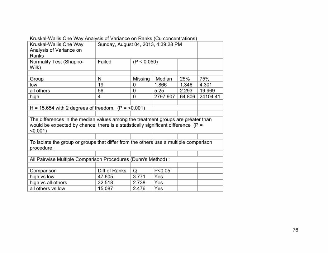
76
Kruskal-Wallis One Way Analysis of Variance on Ranks (Cu concentrations) Kruskal-Wallis One Way Analysis of Variance on Ranks
Sunday, August 04, 2013, 4:39:28 PM
Normality Test (Shapiro-Wilk)
Failed (P < 0.050)
Group N Missing Median 25% 75% low 19 0 1.866 1.346 4.301 all others 56 0 5.25 2.293 19.969 high 4 0 2797.907 64.806 24104.41 H = 15.654 with 2 degrees of freedom. (P = <0.001) The differences in the median values among the treatment groups are greater than would be expected by chance; there is a statistically significant difference (P = <0.001) To isolate the group or groups that differ from the others use a multiple comparison procedure. All Pairwise Multiple Comparison Procedures (Dunn's Method) : Comparison Diff of Ranks Q P<0.05 high vs low 47.605 3.771 Yes high vs all others 32.518 2.738 Yes all others vs low 15.087 2.476 Yes

77

78
Summary Statistics for Copper Concentration Grouped Categories Grouped category:
low all others high
Sample Category in Groups:
Al ramp brick wall concrete plaster roof
artificial turf galv bare galv painted galv coated metal bare metal painted rubber wood bare wood painted
barge hull wood treated
number 19 47 4 min 1 0 27 max 81 174 30334 average 7 21 8989 median 2 4 2798 st dev 18 39 14449 COV 2.7 1.8 1.6

79
Copper Washdown Mass (µg/ft2) Grouped Category:
others others low low others low others high others others low low others others others high
Sample Category:
Al ramp
artificial turf
brick wall
concrete galv bare
galv painted
galv coated
barge hull
metal bare
metal painted
plaster roof rubber wood bare
wood painted
wood treated
9 88 2 77 5 5 24 28,703 7 40 2 3 1 16 6 5,125
2 2 6 54 12 1 4 33 153
2 28 2 1 4 1 1 7 34
3 7 4 122 1 29
1 7 5 9 1 16
2 1 4 3
4 4 237
8 131 420
3 34 3
93 2
164 2
44 2
1
2
16
2
1
95
0
9
4
0
0
3
3
3
Grouped Category:
others others low low others low others high others others low low others others others high
Sample Category:
Al ramp
artificial turf
brick wall
concrete galv bare
galv painted
galv coated
barge hull
metal bare
metal painted
plaster roof rubber wood bare
wood painted
wood treated
number 1 1 1 9 12 3 1 1 5 26 3 5 6 1 1 3

80
min 1 1 2 1 0 1 1 1 34
max 77 164 6 54 420 2 4 33 5,125
average 11 43 4 14 38 2 2 15 1,771
median 9 88 2 3 17 5 24 28,703 5 3 1 1 11 16 6 153
st dev 25 56 2 22 94 0 2 13 2,906
COV 2.2 1.3 0.5 1.6 2.5 0.2 0.8 0.9 1.6

81

82
Kruskal-Wallis One Way Analysis of Variance on Ranks (Cu mass) Normality Test (Shapiro-Wilk)
Failed (P < 0.050)
Group N Missing Median 25% 75% low 21 0 2.133 1.37 3.848 others 54 0 6.198 2.395 30.124 high 4 0 2639.045 63.388 22808.8 H = 16.060 with 2 degrees of freedom. (P = <0.001) The differences in the median values among the treatment groups are greater than would be expected by chance; there is a statistically significant difference (P = <0.001) To isolate the group or groups that differ from the others use a multiple comparison procedure. All Pairwise Multiple Comparison Procedures (Dunn's Method) : Comparison Diff of
Ranks Q P<0.05
high vs low 46.595 3.722 Yes high vs others 30.889 2.597 Yes others vs low 15.706 2.661 Yes Note: The multiple comparisons on ranks do not include an adjustment for ties.

83

84
Summary Statistics for Copper Mass Grouped Categories Grouped Category:
low others high
Sample Categories in Groups:
brick wall concrete galv painted plaster roof
Al ramp artificial turf galv bare galv coated metal bare metal painted rubber wood bare wood painted
barge hull wood treated
number 21 54 4 min 1 0 34 max 77 420 28,703 average 6 34 8,504 median 2 6 2,639 st dev 16 71 13,674 COV 2.6 2.1 1.6

85
Iron Iron Washdown Concentrations (µg/L) Fe (µg/L) low high low other other other high other low low low high other
Al ramp artificial turf
brick wall
concrete galv bare
galv painted
barge hull
metal bare
metal painted
roof rubber wood bare
wood treated
78 769 90 227 71 480 5,995 373 16 281 59 1,135 269
783 6 399 393 6 103
158 4 28 81
63 1,571 10
4 46
332 1,301
74 74
131 412
1,258 6
938
13
5
2
Grouped Category: low high low other other other high other low low low high other
Fe (µg/L) Al ramp artificial turf
brick wall
concrete galv bare
galv painted
barge hull
metal bare
metal painted
roof rubber wood bare
wood treated
number 1 1 1 1 9 2 1 4 13 2 3 1 1
min 4 6 4 2 6 59
max 1,258 480 1,571 1,301 281 103
average 319 243 587 249 143 81
median 78 769 90 227 131 243 5,995 386 28 143 81 1,135 269
st dev 425 335 680 418 194 22
COV 1.3 1.4 1.2 1.7 1.4 0.3

86

87
Kruskal-Wallis One Way Analysis of Variance on Ranks (Fe concentrations) Normality Test (Shapiro-Wilk)
Failed (P < 0.050)
Group N Missing Median 25% 75% low 20 0 66.461 10.813 236.464 others 12 0 144.818 64.608 443.176 high 3 0 1134.599 768.534 5995.28 H = 7.405 with 2 degrees of freedom. (P = 0.025) The differences in the median values among the treatment groups are greater than would be expected by chance; there is a statistically significant difference (P = 0.025) To isolate the group or groups that differ from the others use a multiple comparison procedure. All Pairwise Multiple Comparison Procedures (Dunn's Method) : Comparison Diff of Ranks Q P<0.05 high vs low 16.9 2.664 Yes high vs others 12.667 1.915 No others vs low 4.233 1.131 No Note: The multiple comparisons on ranks do not include an adjustment for ties.

88

89
Summary Statistics for Iron Concentration Grouped Categories Grouped category:
low others high
Sample Category in Groups:
Al ramp brick wall metal painted roof rubber
concrete galv bare galv painted metal bare wood treated
artificial turf barge hull wood bare
number 20 12 3 min 2 4 769 max 1,301 1,258 5,995 average 197 299 2,633 median 66 145 1,135 st dev 344 378 2,918 COV 1.7 1.3 1.1

90
Iron Washdown Mass (µg/ft2) low other low other other other high other low low low high other
Al ramp artificial turf
brick wall
concrete
galv bare
galv painted
barge hull
metal bare
metal painted
roof rubber wood bare
wood treated
157 727 85 286 267 372 5,673 471 15 199 56 1,074 254
741 6 378 949 6 165
150 5 26 76
190 1,882 10
3 110
839 3,282
212 70
265 2,078
1,191 5
710
30
5
2
low other low other other other high other low low low high other
Al ramp artificial turf
brick wall
concrete
galv bare
galv painted
barge hull
metal bare
metal painted
roof rubber wood bare
wood treated
number 1 1 1 1 9 2 1 4 13 2 3 1 1
min 3 6 5 2 6 56
max 1,191 372 1,882 3,282 199 165
average 429 189 684 561 103 99
median 157 727 85 286 265 189 5,673 424 30 103 76 1,074 254
st dev 397 259 824 1,018 137 58
COV 0.9 1.4 1.2 1.8 1.3 0.6
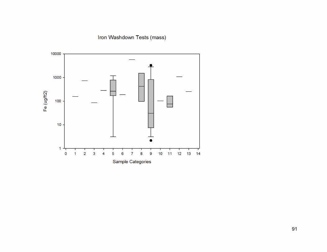
91

92
Kruskal-Wallis One Way Analysis of Variance on Ranks (Fe mass) Normality Test (Shapiro-Wilk)
Failed (P < 0.050)
Group N Missing Median 25% 75% low 20 0 73.065 11.011 190.947 others 18 0 276.548 179.659 730.653 high 2 0 3373.324 1073.614 5673.034 H = 8.140 with 2 degrees of freedom. (P = 0.017) The differences in the median values among the treatment groups are greater than would be expected by chance; there is a statistically significant difference (P = 0.017) To isolate the group or groups that differ from the others use a multiple comparison procedure. All Pairwise Multiple Comparison Procedures (Dunn's Method) : Comparison Diff of
Ranks Q P<0.05
high vs low 21.35 2.463 Yes high vs others 14.056 1.613 No others vs low 7.294 1.921 No Note: The multiple comparisons on ranks do not include an adjustment for ties.

93

94
Summary Statistics for Iron Mass Grouped Categories Grouped Category:
low others high
Sample Categories in Groups:
Al ramp brick wall metal painted roof rubber
artificial turf concrete galv bare galv painted metal bare wood treated
barge hull wood bare
number 20 18 2 min 2 3 1,074 max 3,282 1,882 5,673 average 402 458 3,373 median 73 277 3,373 st dev 840 477 3,252 COV 2.1 1.0 1.0

95
Lead Lead Washdown Concentrations (µg/L) Grouped Category: other other low other other high other other low low other other low
Sample Category: Al ramp artificial turf
brick wall concrete galv bare
galv painted
barge hull
metal bare
metal painted
roof rubber wood bare
wood treated
3.4 6.2 1.4 2.4 1.4 764.0 31.9 0.3 0.2 2.2 0.9 6.0 1.1
46.2 1.5 50.7 3.6 0.2 38.5
2.7 17.1 0.7 1.7
12.1 0.9 0.5
4.2 2.1
14.6 45.3
6.4 0.2
10.5 1.8
2.4 0.2
6.7
0.3
0.2
0.2
Grouped Category: other other low other other high other other low low other other low
Pb (µg/L) Al ramp artificial turf
brick wall concrete galv bare
galv painted
barge hull
metal bare
metal painted
roof rubber wood bare
wood treated
number 1 1 1 1 9 2 1 4 13 2 3 1 1
min 1.4 1.5 0.3 0.2 0.2 0.9
max 46.2 764.0 50.7 45.3 2.2 38.5
average 11.2 382.8 17.3 4.8 1.2 13.7
median 3.4 6.2 1.4 2.4 6.4 382.8 31.9 9.0 0.5 1.2 1.7 6.0 1.1
st dev 13.9 539.2 23.6 12.3 1.4 21.5
COV 1.2 1.4 1.4 2.6 1.2 1.6

96
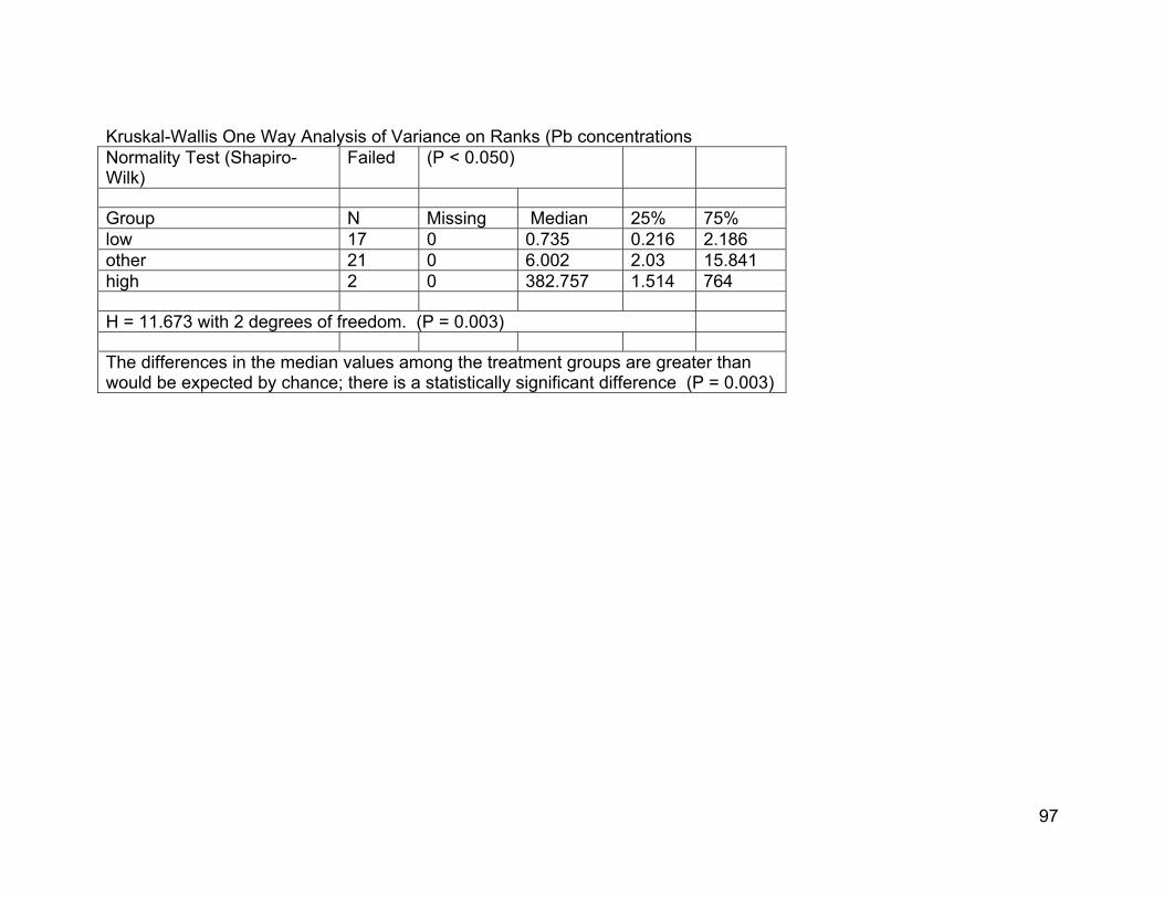
97
Kruskal-Wallis One Way Analysis of Variance on Ranks (Pb concentrations Normality Test (Shapiro-Wilk)
Failed (P < 0.050)
Group N Missing Median 25% 75% low 17 0 0.735 0.216 2.186 other 21 0 6.002 2.03 15.841 high 2 0 382.757 1.514 764 H = 11.673 with 2 degrees of freedom. (P = 0.003) The differences in the median values among the treatment groups are greater than would be expected by chance; there is a statistically significant difference (P = 0.003)
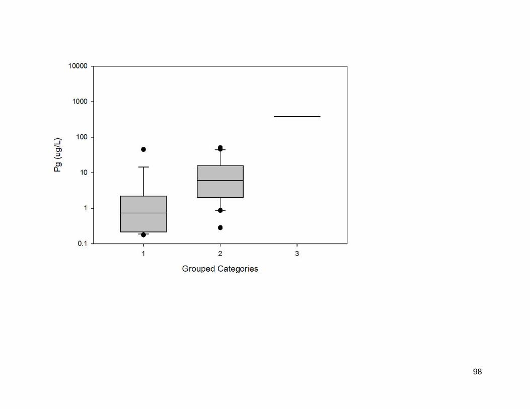
98

99
Summary Statistics for Lead Concentration Grouped Categories Grouped category:
low others high
Sample Category in Groups:
brick wall metal painted roof wood treated
Al ramp artificial turf concrete galv bare barge hull metal bare rubber wood bare
galv painted
number 17 21 2 min 0.2 0.3 1.5 max 45.3 50.7 764.0 average 3.9 12.4 382.8 median 0.7 6.0 382.8 st dev 10.8 15.7 539.2 COV 2.7 1.3 1.4

100
Lead Washdown Mass (µg/ft2) Grouped Category: other other low other other high other other low low other other low
Sample Category: Al ramp artificial turf
brick wall
concrete galv bare galv painted
barge hull
metal bare metal painted
roof rubber wood bare
wood treated
6.9 5.8 1.4 3.1 5.5 592.6 30.2 0.4 0.2 1.6 0.9 5.7 1.0
43.7 1.4 48.0 8.7 0.2 61.8
2.6 19.5 0.7 1.6
36.7 1.0 0.4
3.6 5.2
36.7 114.4
18.1 0.2
21.1 8.8
2.3 0.2
5.1
0.7
0.2
0.2
Grouped Category: other other low other other high other other low low other other low
Sample Category: Al ramp artificial turf
brick wall
concrete galv bare galv painted
barge hull
metal bare metal painted
roof rubber wood bare
wood treated
number 1 1 1 1 9 2 1 4 13 2 3 1 1
min 2.3 1.4 0.4 0.2 0.2 0.9
max 43.7 592.6 48.0 114.4 1.6 61.8
average 18.9 297.0 17.2 11.2 0.9 21.4
median 6.9 5.8 1.4 3.1 18.1 297.0 30.2 10.2 0.7 0.9 1.6 5.7 1.0
st dev 16.6 418.0 22.4 31.2 1.0 35.0
COV 0.9 1.4 1.3 2.8 1.1 1.6

101

102
Kruskal-Wallis One Way Analysis of Variance on Ranks (Pb mass Normality Test (Shapiro-Wilk)
Failed (P < 0.050)
Group N Missing Median 25% 75% low 17 0 0.705 0.204 5.129 others 21 0 5.82 2.438 33.43 high 2 0 297.001 1.433 592.57 H = 10.049 with 2 degrees of freedom. (P = 0.007) The differences in the median values among the treatment groups are greater than would be expected by chance; there is a statistically significant difference (P = 0.007)

103

104
Summary Statistics for Lead Mass Grouped Categories Grouped Category:
low others high
Sample Categories in Groups:
brick wall metal painted roof wood treated
Al ramp artificial turf concrete galv bare barge hull metal bare rubber wood bare
galv painted
number 17 21 2 min 0.2 0.4 1.4 max 114.4 61.8 592.6 average 8.8 16.9 297.0 median 0.7 5.8 297.0 st dev 27.4 18.7 418.0 COV 3.1 1.1 1.4
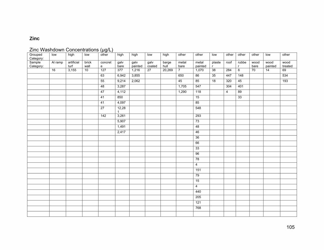
105
Zinc Zinc Washdown Concentrations (µg/L) Grouped Category:
low high low other high high low high other other low other other other low other
Sample Category:
Al ramp artificial turf
brick wall
concrete
galv bare
galv painted
galv coated
barge hull
metal bare
metal painted
plaster
roof rubber
wood bare
wood painted
wood treated
16 3,155 10 127 377 1,216 27 20,269 7 1,070 38 284 6 70 14 69
63 6,942 3,855 650 86 35 447 148 534
55 9,214 2,062 45 85 18 320 45 193
48 3,287 1,705 547 304 401
47 4,112 1,290 118 4 89
41 850 15 33
41 4,097 85
27 12,281
548
142 3,261 293
5,907 73
1,491 48
2,417 46
36
66
33
96
78
4
151
79
15
4
440
205
121
768

106
Grouped Category:
low high low other high high low high other other low other other other low other
Sample Category:
Al ramp artificial turf
brick wall
concrete
galv bare
galv painted
galv coated
barge hull
metal bare
metal painted
plaster
roof rubber
wood bare
wood painted
wood treated
number 1 1 1 9 12 3 1 1 5 26 3 5 6 1 1 3
min 27 377 1,216 7 4 18 4 6 69
max 142 12,281
3,855 1,705 1,070 38 447 401 534
average 66 4,520 2,378 740 197 30 272 120 265
median 16 3,155 10 48 3,692 2,062 27 20,269 650 85 35 304 67 70 14 193
st dev 40 3,539 1,347 752 266 11 163 146 241
COV 0.6 0.8 0.6 1.0 1.4 0.4 0.6 1.2 0.9

107

108
Kruskal-Wallis One Way Analysis of Variance on Ranks (Zn concentrations) Normality Test (Shapiro-Wilk)
Failed (P < 0.050)
Group N Missing Median 25% 75% low 7 0 18.094 14.203 35.11 others 55 0 84.609 44.581 292.835 high 17 0 3286.721 1776.302 6424.577 H = 43.131 with 2 degrees of freedom. (P = <0.001) The differences in the median values among the treatment groups are greater than would be expected by chance; there is a statistically significant difference (P = <0.001) To isolate the group or groups that differ from the others use a multiple comparison procedure. All Pairwise Multiple Comparison Procedures (Dunn's Method) : Comparison Diff of
Ranks Q P<0.05
high vs low 58.429 5.669 Yes high vs others 35.655 5.599 Yes others vs low 22.774 2.473 Yes Note: The multiple comparisons on ranks do not include an adjustment for ties.

109

110
Summary Statistics for Zinc Concentration Grouped Categories Grouped category:
low all others high
Sample Category in Groups:
Al ramp brick wall galv coated plaster wood painted
concrete metal bare metal painted roof rubber wood bare wood treated
artificial turf galv bare galv painted barge hull
number 7 51 17 min 10 4 377 max 38 1,705 20,269 average 23 225 4,988 median 18 85 3,287 st dev 11 343 5,008 COV 0.5 1.5 1.0

111
Zinc Washdown Mass (µg/ft2) Grouped Category:
low high low low high high low high other other low other other other low other
Sample Category:
Al ramp artificial turf
brick wall
concrete
galv bare
galv painted
galv coated
barge hull
metal bare
metal painted
plaster
roof rubber
wood bare
wood painted
wood treated
32 2,986 9 120 1,427 944 45 19,180 9 1,012 36 202 6 66 13 66
79 5,375 1,824 1,221 89 33 353 237 455
70 8,719 1,951 739 80 17 253 54 243
61 3,110 54 1,319 240 343
59 12,451 111 4 124
52 743 14 31
52 5,169 206
34 30,990 1,382
135 9,279 727
20,123 222
1,411 55
4,879 36
1,613 35
41
44
31
78
395
4
115
191
14
4
416
194
114

112
Grouped Category:
low high low low high high low high other other low other other other low other
Sample Category:
Al ramp artificial turf
brick wall
concrete
galv bare
galv painted
galv coated
barge hull
metal bare
metal painted
plaster
roof rubber
wood bare
wood painted
wood treated
number 1 1 1 9 13 3 1 1 4 26 3 5 6 1 1 3
min 34 743 944 9 4 17 4 6 66
max 135 30,990 1,951 1,221 1,382 36 353 343 455
average 73 8,099 1,573 506 267 29 210 132 254
median 32 2,986 9 61 5,169 1,824 45 19,180 397 100 33 240 89 66 13 243
st dev 33 8,784 549 582 396 10 128 132 195
COV 0.5 1.1 0.3 1.2 1.5 0.4 0.6 1.0 0.8

113

114
Kruskal-Wallis One Way Analysis of Variance on Ranks (Zn mass) Normality Test (Shapiro-Wilk)
Failed (P < 0.050)
Group N Missing Median 25% 75% low 16 0 48.381 32.152 67.343 others 45 0 114.072 38.359 297.853 high 18 0 3994.475 1566.44 10072.18 H = 43.608 with 2 degrees of freedom. (P = <0.001) The differences in the median values among the treatment groups are greater than would be expected by chance; there is a statistically significant difference (P = <0.001) To isolate the group or groups that differ from the others use a multiple comparison procedure. All Pairwise Multiple Comparison Procedures (Dunn's Method) : Comparison Diff of Ranks Q P<0.05 high vs low 48.306 6.126 Yes high vs others 35.589 5.561 Yes others vs low 12.717 1.904 No Note: The multiple comparisons on ranks do not include an adjustment for ties.

115

116
Summary Statistics for Zinc Mass Grouped Categories Grouped Category:
low others high
Sample Categories in Groups:
Al ramp brick wall concrete galv coated plaster wood painted
metal bare metal painted roof rubber wood bare wood treated
artificial turf galv bare galv painted barge hull
number 16 45 18 min 9 4 743 max 135 1,382 30,990 average 53 258 7,343 median 48 114 3,994 st dev 35 355 8,377 COV 0.7 1.4 1.1

117
Summary of Washoff Tests Due to the varying number of observations for the different material categories, some of the test statistics are incomplete, but they do enable the identification of the types of materials of greatest interest. The following table summarizes the “low,” “other,” and “high” categories for each sample type and metal. In almost all cases, the concentration and mass washoff categories are the same; for the few that differ, the differences are not large (low/other or other/high). Most of these groupings are obvious and as expected, such as the bare galvanized metal being the highest category for zinc, and the aluminum ramp being the highest for aluminum. Other findings are interesting and potentially important, such as:
Aluminum ramp high for aluminum (as expected) Artificial turf high for zinc and possibly high for iron, possibly due to
recycled rubber tire crumbles used to support artificial grass leaves Bare galvanized metal high for zinc (as expected) Painted galvanized metal high for zinc, and high for aluminum and lead
(the aluminum and lead are higher than for bare galvanized materials, likely due to the metal primers or paints; coated galvanized metals were much lower for all metals)
Barge hull high for zinc, copper, and iron, possibly associated with anti-fouling paints
Bare wood high for aluminum and iron Treated wood high for copper (as expected)
The high metals associated the artificial turf and the high metals associated with the barge hull are important findings, but are only represented by single samples. Additional sample collections representing these two categories are therefore highly recommended to determine if these findings are consistent.
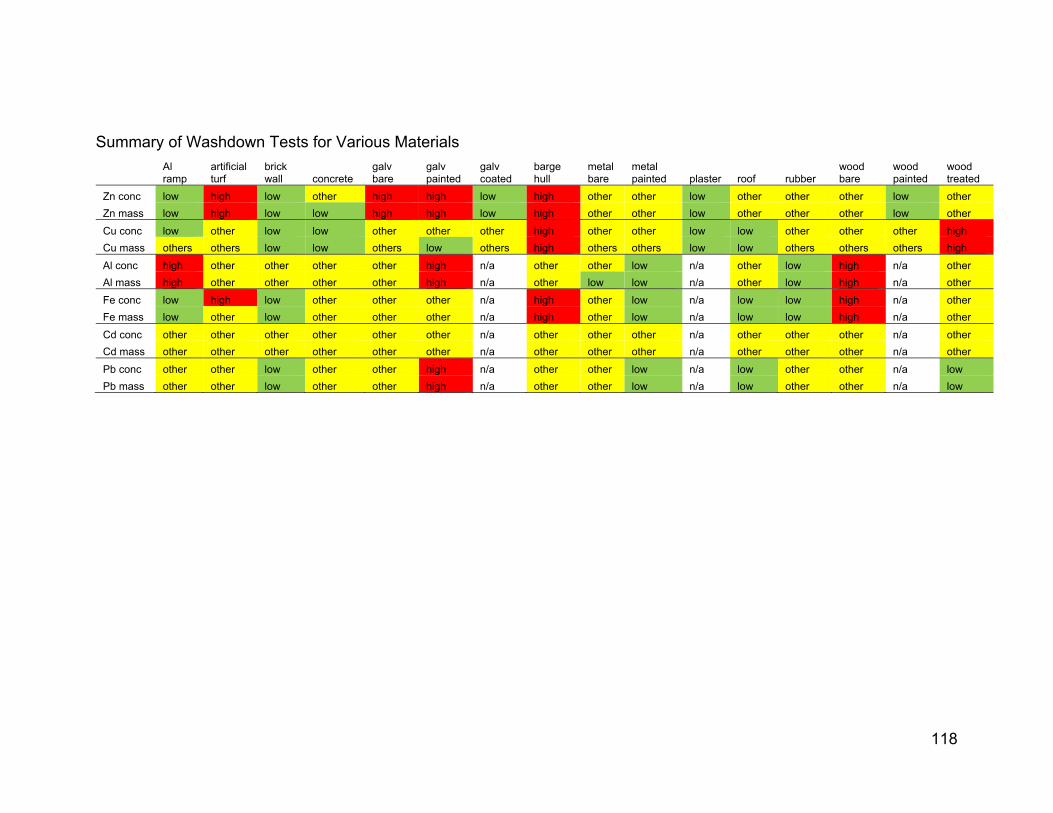
118
Summary of Washdown Tests for Various Materials
Al ramp
artificial turf
brick wall concrete
galv bare
galv painted
galv coated
barge hull
metal bare
metal painted plaster roof rubber
wood bare
wood painted
wood treated
Zn conc low high low other high high low high other other low other other other low other
Zn mass low high low low high high low high other other low other other other low other
Cu conc low other low low other other other high other other low low other other other high
Cu mass others others low low others low others high others others low low others others others high
Al conc high other other other other high n/a other other low n/a other low high n/a other
Al mass high other other other other high n/a other low low n/a other low high n/a other
Fe conc low high low other other other n/a high other low n/a low low high n/a other
Fe mass low other low other other other n/a high other low n/a low low high n/a other
Cd conc other other other other other other n/a other other other n/a other other other n/a other
Cd mass other other other other other other n/a other other other n/a other other other n/a other
Pb conc other other low other other high n/a other other low n/a low other other n/a low
Pb mass other other low other other high n/a other other low n/a low other other n/a low

119
Contaminated Soils Analyses at Navy Facilities In addition to the washoff tests described above, SPARWARS-PACIFIC personnel also collected several soil and sediment samples, especially from likely contaminated areas. The following photographs are examples of some of these sampling activities.
Contaminated dry soil sampling. Clean dry soil sampling.
Sampling of accumulated sediment near inlet.
Sampling of sediment in ponded water.

120
Comparison of Recent Navy Facility Source Area Water Quality Observations with Other Data (WinSLAMM Calibration File Preparation) The following tables summarize the literature information, along with recent short-term leachate results, and recent washoff test results for different materials likely exposed to rainwater and stormwater. These results are shown as concentrations and as mass losses. The results are not directly comparable due to the different testing conditions used (water chemistries, water volumes, and contact times), but do illustrate typical concentrations that have been observed and identify the most consistently problematic materials. The most common material associated with elevated heavy metal concentrations are galvanized metals: painted or bare galvanized steel and galvanized aluminum resulting in very high zinc concentrations. The single test for artificial turf also resulted in very high zinc concentrations. Factory coated galvanized materials are shown to usually have much lower resulting zinc concentrations in the leachate or washoff water, if the coatings are in good condition. Any exposed copper (especially aged patinated copper) also results in very high copper concentrations, but these materials are most likely limited to older roof flashings. Treated wood and special paints used on ship hulls (based on a single barge hull analysis) also result in elevated copper concentrations. High lead concentrations were reported in the literature and observed during the washoff tests associated with uncoated galvanized materials and some water distribution systems. Some high cadmium concentrations were observed associated with uncoated galvanized steel and drinking water systems. Very high iron concentrations were associated with uncoated galvanized materials, bare wood and painted barge hull (single samples). The highest aluminum concentrations were associated with the exposed aluminum materials and painted galvanized metals. During the controlled leachate tests, almost all metal concentrations increased dramatically with increased exposure times. The data presented in this section focused on one hour exposure periods, but if materials were exposed for extended periods (such as for water storage tanks or if materials were in ponds or small puddles), then the concentrations could be more than 100 times higher than indicated here. In addition, in most cases, reduced pH (about 5) resulted in much greater concentrations compared to higher pH (about 8) conditions. Lower pH would be associated with roof exposures, while higher pH occurs after runoff flows across most surfaces or is discharged into receiving waters. These data are used in developing the special WinSLAMM categories for material exposures (mainly exposed galvanized metals and scrapyard/storage yard contaminated soils) and associated expected concentrations from those areas.

121
Literature, Leaching Tests, and Washoff Data Comparisons for Zinc uncoated galvanized steel coated galvanized steel painted galvanized steel uncoated galvanized
aluminum coated galvanized aluminum
water systems with some galv pipe
concentration (µg/L)
mass loss (g/m
2/yr)
concentration (µg/L)
mass loss (g/m
2/yr)
concentration (µg/L)
mass loss (g/m
2/yr)
concentration (µg/L)
mass loss (g/m
2/yr)
concentration (µg/L)
mass loss (g/m
2/yr)
concentration (µg/L)
mass loss (g/m
2/yr)
literature 90 to 30,000 2.4 to 8.5 160 to 30,000 0.07 to 15 n/a n/a 200 to 1,600 n/a 60 to 180 n/a 6 to 2,000 n/a
galvanized steel copper other materials (aluminum, concrete, plastics)
UA (1 hr exposure)
concentration (µg/L)
mass loss (g/m
2)
concentration (µg/L)
mass loss (g/m
2)
concentration (µg/L)
mass loss (g/m
2)
avg 1,600 0.055 15 0.001 11 0.001
range 150 to 2,500 0.005 to 0.15
<10 to 30 0 to 0.002 <10 to 15 0.0005 to 0.002
Navy Washoff Tests
low (Al ramp, brick wall, galv coated, plaster, and wood painted)
others (concrete, metal bare, metal painted, roof, rubber, wood bare, and wood treated)
high (artificial turf, galv bare, galv painted, and barge hull)
concentration (µg/L)
mass loss (g/m
2)
concentration (µg/L)
mass loss (g/m
2)
concentration (µg/L)
mass loss (g/m
2)
avg 23 0.57 53 2.80 5,000 79
range 10 to 38 0.10 to 1.5
4 to 1,700 0.04 to 15 380 to 20,200 8 to 335

122
Literature, Leaching Tests, and Washoff Data Comparisons for Copper Uncoated copper roofing Other roofing materials (galv, Al,
vinyl, shakes) Aged (Patinated) copper Copper pipes
concentration (µg/L)
mass loss (g/m2/yr)
concentration (µg/L)
mass loss (g/m2/yr)
concentration (µg/L)
mass loss (g/m2/yr)
concentration (µg/L)
mass loss (g/m2/yr)
literature 2 to 175 1 to 33 <1 to 250 n/a 900 to 9,000 0.75 to 9 200 to 10,000 3.5 to 8
galvanized steel copper other materials (aluminum, concrete, plastics)
UA (1 hr exposure)
concentration (µg/L)
mass loss (g/m2)
concentration (µg/L)
mass loss (g/m2)
concentration (µg/L)
mass loss (g/m2)
avg <1 0.001 360 0.03 15 <0.001
range <1 <0.001 to 0.004
50 to 1,000 <0.01 to 0.08 <10 to 30 <0.001
Navy Washoff Tests
low (Al ramp, brick wall, concrete, plaster, and roof)
others (artificial turf, galv bare, galv painted, galv coated, metal bare, metal painted, rubber, wood bare, and wood painted)
high (barge hull and wood treated)
concentration (µg/L)
mass loss (g/m2)
concentration (µg/L)
mass loss (g/m2)
concentration (µg/L)
mass loss (g/m2)
avg 7 0.06 21 0.37 9,000 91
range 1 to 81 0.01 to 0.8 0 to 174 0 to 4.5 27 to 30,000 0.4 to 310

123
Literature, Leaching Tests, and Washoff Data Comparisons for Lead uncoated galvanized steel uncoated galvanized
aluminum coated galvanized aluminum painted wood water distribution systems
concentration (µg/L)
mass loss (g/m2/yr)
concentration (µg/L)
mass loss (g/m2/yr)
concentration (µg/L)
mass loss (g/m2/yr)
concentration (µg/L)
mass loss (g/m2/yr)
concentration (µg/L)
mass loss (g/m2/yr)
literature 1 to 2,700 n/a <0.1 to 6 n/a <10 to 200 n/a <2 to 400 n/a <5 to 1,000 n/a
galvanized steel copper other materials (aluminum, concrete, plastics)
UA (1 hr exposure)
concentration (µg/L)
mass loss (g/m2)
concentration (µg/L)
mass loss (g/m2)
concentration (µg/L)
mass loss (g/m2)
avg <5 <0.001 <5 <0.001 <5 <0.001
range <5 <0.001 <5 <0.001 <5 <0.001
Navy Washoff Tests
low (brick wall, metal painted, roof, and wood treated)
others (Al ramp, artificial turf, concrete, galv bare, barge hull, metal bare, rubber, and wood bare)
high (galv painted)
concentration (µg/L)
mass loss (g/m
2) concentration (µg/L)
mass loss (g/m2)
concentration (µg/L)
mass loss (g/m2)
avg 3.9 0.09 12 0.18 380 3.2
range 0.2 to 45 0.002 to 1.2 0.3 to 51 0.004 to 0.7
1.5 to 770 0.015 to 6.4

124
Literature, Leaching Tests, and Washoff Data Comparisons for Cadmium uncoated galvanized steel Drinking water systems
concentration (µg/L)
mass loss (g/m2/yr)
concentration (µg/L)
mass loss (g/m2/yr)
literature <0.02 to 32 15 to 25 <0.02 to 88 n/a
Navy Washoff Tests
all sources
concentration (µg/L)
mass loss (g/m2)
avg 7.7 0.13
range 0.05 to 160 0.0005 to 3.4
Literature, Leaching Tests, and Washoff Data Comparisons for Iron uncoated galvanized aluminum coated galvanized aluminum drinking water systems
concentration (µg/L)
mass loss (g/m2/yr)
concentration (µg/L)
mass loss (g/m2/yr)
concentration (µg/L)
mass loss (g/m2/yr)
literature 18 to 1,700 n/a 6 to 24 n/a 0.06 to 1.4 n/a
Navy Washoff Tests
low (Al ramp, brick wall, metal painted, roof, and rubber)
others (artificial turf, concrete, galv bare, galv painted, metal bare, and wood treated)
high (barge hull and wood bare)
concentration (µg/L)
mass loss (g/m2)
concentration (µg/L)
mass loss (g/m2)
concentration (µg/L)
mass loss (g/m2)
avg 200 4.3 300 4.9 2600 36.6
range 2 to 1,300 0.02 to 36 4 to 1,260 0.03 to 21 770 to 6,000 12 to 62

125
Literature, Leaching Tests, and Washoff Data Comparisons for Aluminum Navy Washoff Tests
low (metal painted and rubber) others (artificial turf, brick wall, concrete, galv bare, barge hull, metal bare, roof, and wood treated)
high (Al ramp and galv painted)
concentration (µg/L)
mass loss (g/m2)
concentration (µg/L)
mass loss (g/m2)
concentration (µg/L)
mass loss (g/m2)
avg 172 3.1 230 3.2 770 9.0
range 1.8 to 1,400 0.02 to 37 2.4 to 1,200 0.023 to 12 4 to 1,800 0.04 to 15
126
Trace Heavy Metal Treatability The form of the pollutant species plays an important role in selecting an appropriate treatment technology (Clark and Pitt 2012). Many heavy metals are associated predominantly with particulates, and therefore their treatability is influenced by the removal of the associated particulates. The association of heavy metals with particulates depends on pH, oxidation-reduction potential, particulate organic matter. The treatability of stormwater solids and associated heavy metals is dependent on their size (Morquecho, et al. 2005; House, et al. 1993; Li, et al. 2005; Kim and Sansalone, 2008). Sedimentation and physical filtration can be used to remove the particulates with the attached pollutants from stormwater (Pitt, et al. 1996). For sedimentation, the median suspended solids removal efficiency is between 70 and 80% (Clark and Pitt 2012; Hossain, et al. 2005; International Stormwater BMP Database 2011). The sedimentation effectiveness is dependent upon the size of suspended solids. The removal of large suspended solids is efficient; however the suspended solids removal diminishes with the increase of content of smaller particulates (Clark and Pitt 2012; Greb and Bannerman, 1997). The heavy metal removal by sedimentation is very efficient at locations where the particulates are large (highways, for example) and the heavy metals are predominantly associated with the larger particulates (Clark and Pitt 2012; Kim and Sansalone, 2008). Effectively designed wet detention ponds have restricted short-circuiting and low surface overflow rates (SOR). The sedimentation basins are not very effective for the removal of very small particles (< 2 μm) due to the repulsive forces caused by the negative charges on colloids and clay-sized particles that keep solids in suspension and prevent the particles from settling (Clark and Pitt 2012). The sedimentation can be improved by coagulation/flocculation that neutralized the electrical charges on the particles and causes the solids to settle out. Testing will be necessary since it is impossible to predict the settling of the floc theoretically (Clark and Pitt 2012; Metcalf and Eddy, 2003). For metals that are predominantly associated with particles in the range of colloidal and clay particles (< 1 µm), filtration with a chemically-active media may be necessary if low numeric discharge limits must be met (Clark and Pitt 2012; Pitt and Clark 2010). Sand with oxide coatings can be used to remove colloidal pollutants (Clark and Pitt 2012; Sansalone and Kim 2006). The removal of dissolved contaminants may be needed due to their high mobility and to meet permit requirements and reduce surface and groundwater contamination potential (Pitt, et al. 1996; Clark and Pitt 2012). Heavy metals in ionic forms are the most bioavailable. The toxicity of a heavy metal is affected by metal bioavailability which is controlled by speciation and partitioning of a metal. Metals in ionic forms are generally more bioreactive than metal complexes. Treatment techniques for metals associated with dissolved fractions include chemical treatment. To remove dissolved metals from stormwater, organic filter media (such as compost or peat), a mix of peat moss and sand, zeolite, and compost can be used. Zn2+ is highly reactive and is more amenable to ion exchange.

127
In physisorption reactions, the electrical bonds between the contaminants and the media are reversible and weak. On the other hand, during chemisorption and precipitation reactions stronger bonds are formed and the pollutant retention is permanent if the solution pH and dissolved oxygen level do not change significantly (Evangelou, 1998; Watts, 1998; Clark and Pitt 2012). Sorption and ion exchange remove pollutants through electrostatic interactions between the media and contaminants (Clark and Pitt 2012). The high sodium content during the snowmelt can regenerate the ion exchanging media and release the already retained heavy metals back into the effluent (Clark and Pitt 2012), in addition to increasing the sodium adsorption ratio (SAR) that can greatly hinder infiltration rates in soils or media having even small amounts of clay. Granular activated carbon (GAC) technology is costly and therefore is not regularly used for stormwater applications, but is used when very low permit limits must be met (Pitt and Clark 2012). The valence charge of a metal and its complexation, among other contaminant properties, influence the choice of stormwater treatment technology (Clark and Pitt 2012). Strongly charged, small molecules can be removed effectively by zeolites (Clark and Pitt 2011 and 2012). Zeolites are not effective in the removal of compounds of zero valence and compounds with large size (Clark and Pitt 2012). Peat, compost and soils remove pollutants by chemisorption that is generally irreversible (Watts 1998; Evangelou 1998). Peat can be used as a filtration media for treatment of heavy metals and likely their complexes (Clark and Pitt 2012 and 1999). Peat’s effectiveness is due to the wide range of binding sites (carboxylic acid, etc.) present in the humic materials and ligands in the peat (Cohen, et. Al. 1991; Sharma and Foster 1993; Clark and Pitt 2012). An advantage of peat media is that it can treat many heavy metals during relatively short (10 minutes) contact times (Pitt and Clark 2010; Clark and Pitt 2012). The peat’s drawbacks (especially for Sphagnum peat) includes the leaching of colored humic and fulvic acids and the release of hydronium ions (H3O
+) in exchange for metals which can lower the pH of the treated water by as much as 1 to 2 pH units and increase the solubility of the metals that were associated with stormwater runoff solids or media (Clark and Pitt 2012, 1999). Another disadvantage of using peat is the release of nutrients from the filter during the first flush under microanaerobic conditions in the media which may occur between storms (Clark and Pitt 2009b), although this is not as problematic as for compost media. Compost (including municipal leaf waste compost) can also be used to treat metals (Sharma and Foster 1993; Guisquiani, et al. 1995). The advantage of compost is that it is not likely to reduce the pH of the treated water (Clark and Pitt 1999). However, the disadvantage is that it can release nutrients, depending on the compost’s source material, during the first few years of its life (Hathaway, et al. 2008, Pitt, et al. 1999; Pitt and Clark 2010). Treatment trains, like the multi-chambered treatment train (MCTT) can be effectively used for metal treatment and include catch basins for retaining the largest sediment, settling chambers for retaining fine sediment and particle-bound pollutants, and an sorption/ion exchange chamber with mixed media (peat moss, sand) for capturing filterable contaminants through sorption/ion-exchange (Pitt, et al. 1999). The upflow filter was also found to be an effective method for controlling stormwater and uses sedimentation, screens for floatable solids, sorption, and ion exchange (Togawa and Pitt, available online). Grass swales may be effective

128
for removing metals. They capture heavy metals by sedimentation, infiltration/sorption, and biological uptake, can treat high volumes of water and are relatively inexpensive (Johnson, et al. 2003). The data for total and filtered metal concentrations of lead, copper, zinc, and aluminum analyzed after three months of exposure during the buffered tests was compared to estimate metal association with the particulate matter by Ogburn (2013). Analytical methods having smaller detection limits are necessary to account for non-detected values. The following tables summarize particulate and filterable lead and zinc fractions in different samples during the buffered pH tests. Generally, most of the lead was associated with the particulate fraction under pH 5 conditions and with the dissolved fraction (> 76%) under pH 8 conditions during the buffered tests after three months of exposure. For pH 5 waters, no detectable concentrations of lead were associated with the dissolved fraction. Under pH 8 conditions, most of the lead was associated with the dissolved fraction, while24% of the lead was associated with particulates for galvanized steel pipe, and only 4% for galvanized steel gutter. Filterable and particulate fractions of lead and zinc in buffered waters after three months of exposure (Ogburn 2013)
Water Material %
Filterable Pb
% Particulate
Pb
% Filterable
Zn
% Particulate
Zn
pH 5
Concrete Pipe n/a n/a n/a n/a PVC Pipe n/a n/a 89 11 HDPE Pipe n/a n/a 83 17 Steel Pipe < 2.0 > 98 24 76 Vinyl Gutter n/a n/a n/a n/a Aluminum Gutter n/a n/a 100 0 Steel Gutter < 13.5 > 86 51 49 Copper Gutter n/a n/a < 15 > 85
pH 8
Concrete Pipe n/a n/a < 67 > 33 PVC Pipe n/a n/a 18 82 HDPE Pipe n/a n/a 100 0 Steel Pipe 76 24 0.34 100 Vinyl Gutter n/a n/a 100 0 Aluminum Gutter n/a n/a 24 76 Steel Gutter 96 4 1.7 98 Copper Gutter n/a n/a 100 0
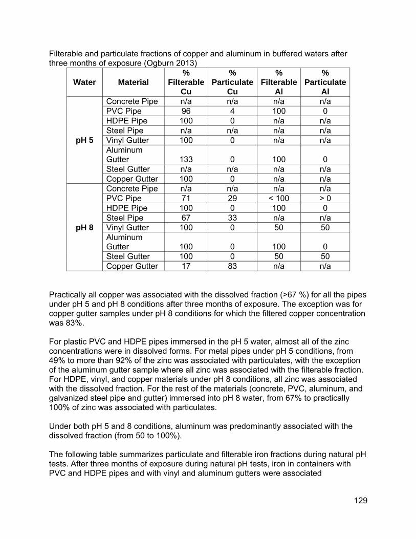
129
Filterable and particulate fractions of copper and aluminum in buffered waters after three months of exposure (Ogburn 2013)
Water Material %
Filterable Cu
% Particulate
Cu
% Filterable
Al
% Particulate
Al
pH 5
Concrete Pipe n/a n/a n/a n/a PVC Pipe 96 4 100 0 HDPE Pipe 100 0 n/a n/a Steel Pipe n/a n/a n/a n/a Vinyl Gutter 100 0 n/a n/a Aluminum Gutter 133 0 100 0 Steel Gutter n/a n/a n/a n/a Copper Gutter 100 0 n/a n/a
pH 8
Concrete Pipe n/a n/a n/a n/a PVC Pipe 71 29 < 100 > 0 HDPE Pipe 100 0 100 0 Steel Pipe 67 33 n/a n/a Vinyl Gutter 100 0 50 50 Aluminum Gutter 100 0 100 0 Steel Gutter 100 0 50 50 Copper Gutter 17 83 n/a n/a
Practically all copper was associated with the dissolved fraction (>67 %) for all the pipes under pH 5 and pH 8 conditions after three months of exposure. The exception was for copper gutter samples under pH 8 conditions for which the filtered copper concentration was 83%. For plastic PVC and HDPE pipes immersed in the pH 5 water, almost all of the zinc concentrations were in dissolved forms. For metal pipes under pH 5 conditions, from 49% to more than 92% of the zinc was associated with particulates, with the exception of the aluminum gutter sample where all zinc was associated with the filterable fraction. For HDPE, vinyl, and copper materials under pH 8 conditions, all zinc was associated with the dissolved fraction. For the rest of the materials (concrete, PVC, aluminum, and galvanized steel pipe and gutter) immersed into pH 8 water, from 67% to practically 100% of zinc was associated with particulates. Under both pH 5 and 8 conditions, aluminum was predominantly associated with the dissolved fraction (from 50 to 100%). The following table summarizes particulate and filterable iron fractions during natural pH tests. After three months of exposure during natural pH tests, iron in containers with PVC and HDPE pipes and with vinyl and aluminum gutters were associated
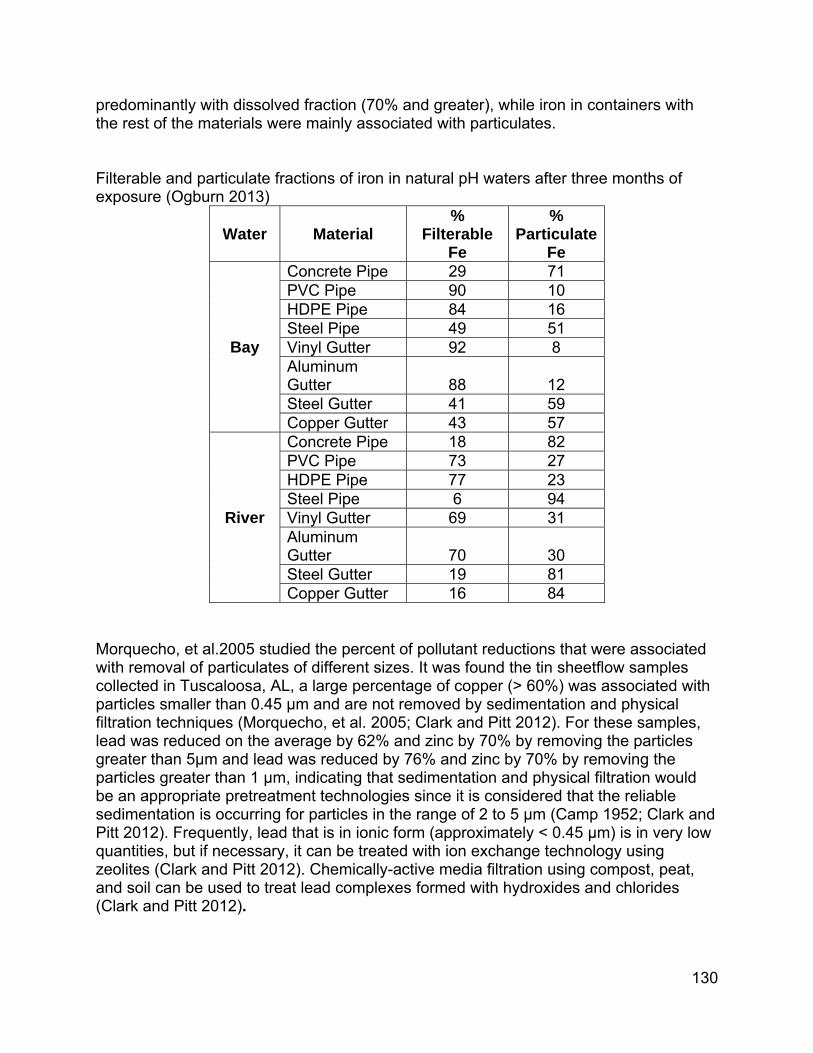
130
predominantly with dissolved fraction (70% and greater), while iron in containers with the rest of the materials were mainly associated with particulates.
Filterable and particulate fractions of iron in natural pH waters after three months of exposure (Ogburn 2013)
Water Material %
Filterable Fe
% Particulate
Fe
Bay
Concrete Pipe 29 71 PVC Pipe 90 10 HDPE Pipe 84 16 Steel Pipe 49 51 Vinyl Gutter 92 8 Aluminum Gutter 88 12 Steel Gutter 41 59 Copper Gutter 43 57
River
Concrete Pipe 18 82 PVC Pipe 73 27 HDPE Pipe 77 23 Steel Pipe 6 94 Vinyl Gutter 69 31 Aluminum Gutter 70 30 Steel Gutter 19 81 Copper Gutter 16 84
Morquecho, et al.2005 studied the percent of pollutant reductions that were associated with removal of particulates of different sizes. It was found the tin sheetflow samples collected in Tuscaloosa, AL, a large percentage of copper (> 60%) was associated with particles smaller than 0.45 µm and are not removed by sedimentation and physical filtration techniques (Morquecho, et al. 2005; Clark and Pitt 2012). For these samples, lead was reduced on the average by 62% and zinc by 70% by removing the particles greater than 5µm and lead was reduced by 76% and zinc by 70% by removing the particles greater than 1 µm, indicating that sedimentation and physical filtration would be an appropriate pretreatment technologies since it is considered that the reliable sedimentation is occurring for particles in the range of 2 to 5 µm (Camp 1952; Clark and Pitt 2012). Frequently, lead that is in ionic form (approximately < 0.45 µm) is in very low quantities, but if necessary, it can be treated with ion exchange technology using zeolites (Clark and Pitt 2012). Chemically-active media filtration using compost, peat, and soil can be used to treat lead complexes formed with hydroxides and chlorides (Clark and Pitt 2012).

131
Zero-valent iron (ZVI) was found to be an efficient medium for treating stormwater heavy metal ions as Cu2+ and Zn2+ (Rangsivek and Jekel 2005, Shokes and Moller 1999; Wilkin and McNeil 2003). Rangsivek and Jekel (2005) found that a significant fraction of Cu2+ is transformed to insoluble CuO and Cu2O species. Zn 2+ is removed by adsorption and co-precipitation with iron oxides. Zero-valent iron removes inorganic pollutants via cementation (reduction of redox sensitive compounds to insoluble forms, for example, Cu2++Fe0Cu0+Fe2+), adsorption and metal hydroxide precipitation (Rangsivek and Jekel 2005, Cantrell, et al. 1995; Shokes and Moller 1999; Blowes, et al. 2000; Naftz, et al. 2002; Wilkin and McNeil 2003). Higher values of water pH, dissolved oxygen (DO), temperature, and ionic strength increased the removal rates of Zn2+. At higher pH values and in the presence of dissolved oxygen (DO), adsorption and co-precipitation with iron oxide are predominantly occur (Rangsivek and Jekel 2005). On the other hand, at low pH values in the absence of DO, the cementation is very effective (Rangsivek and Jekel 2005; Strickland and Lawson 1971; Ku and Chen 1992). ZVI was found to have capacity comparable to a commercial adsorbent granular ferric hydroxide (GFH). The advantages of zero-valent iron (ZVI) are that it is inexpensive and can provide environmental benefits when used in the reclamation of solid waste (Rangsivek and Jekel 2005). Also, ZVI can be installed in an on-site remediation system as a fixed-bed barrier (Morrison, et al. 2002). Drawbacks of ZVI include the release of dissolved iron and complexes of iron oxides with other heavy metals. Therefore, a post-treatment process that includes aeration and sand filtration may be necessary. The removal of such substances as oil from iron’s surfaces may be required if iron was acquired as solid waste. A virgin coconut hull granular activated carbon (GAC), which has a limited chemical capacity, can be used for nitrate (NO3
-) treatment (Pitt and Clark 2010). To remove nitrate and nitrite, vegetated systems can be utilized (Baker and Clark 2012; Lucas and Greenway 2008, 2011; Hunt, et al. 2006; Hunt, et al. 2008). For nitrogen removal, zeolites, commercial resins, and some native soils may be used. Current work on the removal of nitrogen compounds is focusing on denitrification in anaerobic systems and on bacterial processes in subsurface gravel wetlands and biofilters. Sedimentation can be utilized to treat particulate bound phosphorus. To remove phosphorus associated with colloids or are in dissolved forms, vegetative systems may be used (Clark and Pitt 2012). Ionic fractions for zinc, copper, and cadmium can range from 25 to 75% (Clark and Pitt 2012). Sedimentation and physical filtration can be used to treat metals that are bound to particles. These metals can be associated with very small particles, therefore the efficiency of physical filtration to remove metals will depend on size of associated particulates. Treatment technologies for metals associated with dissolved fraction include chemical methods. To remove dissolved metals from stormwater, peat moss, mixtures of peat moss and sand, zeolite, and compost can be used, especially with long contact times. These metals can form soluble complexes with different inorganic and organic ligands. The complex valence can range from -2 to +2. Organic and inorganic

132
complexes may be treated by chemically active filtration through compost, peat, and soil. Also, granular activated carbon (GAC) can be used to remove complexes with organic matter. The choice of treatment methods depends on form of heavy metals and desired level of metal removal. If high degree of metal reduction is required, it is necessary to use multiple techniques (Clark and Pitt 2012). Generally, low numeric discharge limits can be met through combinations of pre-treatment by sedimentation and filtration with a chemically and biologically active media. Summary of Heavy Metal Treatability Many heavy metals are associated predominantly with particulates, and therefore their treatability is influenced by the removal of the associated particulates. The association of heavy metals with particulates depends on pH, oxidation-reduction potential, and particulate organic matter. The treatability of stormwater solids and associated heavy metals is dependent on their size. The removal of dissolved contaminants may be needed to meet stringent numeric discharge permit requirements and reduce surface and groundwater contamination potentials. The valence charge of a metal and its complexation, among other contaminant properties, influence the choice of stormwater treatment technology. Strongly charged, small molecules can be removed effectively by zeolites. Zeolites are not effective in the removal of compounds of zero valence and compounds with large size. Peat can be used as a filtration media for treatment of heavy metals and likely their complexes. Peat’s effectiveness is due to the wide range of binding sites (carboxylic acid, etc.) present in the humic materials and ligands in the peat. An advantage of peat media is that it can treat many heavy metals during relatively short (as short as 10 minutes) contact times. Tests were conducted over a three month exposure period of pipe, gutter, and storage tank materials. Generally, most of the lead was associated with the particulate fraction under pH 5 conditions and with the dissolved fraction (> 76%) under pH 8 conditions after three months of exposure. Practically all copper was associated with the dissolved fraction (>67 %) for all the pipes under pH 5 and pH 8 conditions after three months of exposure. For plastic PVC and HDPE pipes immersed in pH 5 buffered stormwater, almost all of the zinc concentrations were in dissolved forms. For metal pipes under pH 5 conditions, from 49% to more than 92% of the zinc was associated with particulates, with the exception of the aluminum gutter sample where all zinc was associated with the filterable fraction. Prior research found that ionic fractions for zinc, copper, and cadmium in stormwater can range from 25 to 75%. These metals can be associated with very small particles, therefore the efficiency of physical filtration to remove metals will depend on size of associated particulates. Treatment technologies for metals associated with dissolved fractions include chemical methods. To remove dissolved metals from stormwater, peat moss, mixtures of peat moss and sand, zeolite, and compost can be used, especially

133
with long contact times. These metals can form soluble complexes with different inorganic and organic ligands. The complex valences can range from -2 to +2. Organic and inorganic complexes may be treated by chemically active filtration through compost, peat, and soil. Also, granular activated carbon (GAC) can be used to remove complexes with organic matter.

134
References Al-Malack, Muhammad H., Migration of Lead from Unplasticized Polyvinyl Chloride
Pipes. Journal of Hazardous Materials. B82 (2001) 263-274 Baker, K.H., Clark, S.E., Recycling Vertical-Flow Biofilter: A Treatment System for
Agricultural Subsurface Tile Water. In: Garcı´a-Gariza´bal, Iker, Abrahao, Raphael (Eds.), Irrigation–Water Management, Pollution and Alternative Strategies. In Tech, ISBN 978-953-51-0421-6. Available at: http://www.intechopen.com/books/irrigation-water-management-pollution-andalternative-strategies/recycling-vertical-flow-biofilter-atreatment-system-for-agricultural-subsurface-tile-water. 2012.
Bannerman, R., K. Baun, M. Bohn, P.E. Hughes, and D.A. Graczyk. Evaluation of Urban Nonpoint Source Pollution Management in Milwaukee County, Wisconsin, Vol. I. PB 84-114164. U.S. Environmental Protection Agency, Water Planning Division. November 1983.
Blowes, D.W., Ptacek, C.J., Benner, S.G., McRae, C.W.T., Bennett, T.A., Puls, R.W., Treatment of Inorganic Contaminants Using Permeable Reactive Barriers. J. Contam. Hydrol. 45, 123–137. 2000.
Boller, M.A.; Steiner, M. Diffuse Emission and Control of Copper in Urban Surface Runoff. Water Science and Technology, 46(6-7), 173-181. 2002
Burton, G. Allen, Jr., Pitt, Robert E., Stormwater Effects Handbook: A Toolbox for Watershed Managers, Scientists, and Engineers. Lewis Publishers. CRC Press Company. ISBN 0-87371-924-7. 2002.
Camp, T.R. Water treatment. In: Handbook of Applied Hydraulics, 2nd Edition. Edited by C.V. Davis. McGraw-Hill, Inc., New York, NY. 1952
Cantrell, D., D. Kaplan, and T. Wietsma, Zero-valent Iron for the in Situ Remediation of Selected Metals in Groundwater. Environ. Sci. Techno., 42: 201-212, 1995.
Clark, S. and Pitt, R. Stormwater Runoff Treatment: Evaluation of Filtration Media. EPA 600/R-00/010. U.S. Environmental Protection Agency, Water Supply and Water Resources Division, National Risk Management Research Laboratory. EPA/600/R-99/017. Cincinnati, Ohio. 405 pages. 1999
Clark, S., Pitt, R., Burian, S., Field, R., Fan, E., Heaney, J., and Wright, L. Annotated bibliography of urban wet weather flow literature from 1996 to 2006. Available at: http://unix.eng.ua.edu/~rpitt/Publications/Wetweatherlit/1996%20to%202006%20WEF%20lit%20reviews.pdf. 2007
Clark, Shirley E., Long Brett V., Siu Christina Y.S., Spicher Julia, Steele Kelly A., Runoff Quality from Roofing during Early Life. Accepted for publication in the Low Impact Development 2008 Conference Proceedings, Seattle, WA, November 16 – 19, 2008. American Society of Civil Engineers, Reston, VA. CD-ROM. 2008a
Clark, Shirley E., Steele, Kelly A., Spicher, Julia, Siu, Christina Y.S., Lalor, Melinda M., Pitt, Robert, Kirby, Jason T., , Roofing Materials’Contributions to Storm-Water Runoff Pollution. Journal of Irrigation and Drainage Engineerigng.Vol.134, No. 5, October 1, 2008b
Clark, S.E. and Pitt, R. Solids removal in storm-water filters modeled using a power equation. Journal of Environmental Engineering 135(9):896-899. 2009a

135
Clark, S.E. and Pitt, R. Filter media pollutant retention under aerobic versus anaerobic conditions. Journal of Environmental Engineering 135(5):367-371. 2009b
Clark, S.E. and Pitt, R. Filtered metals control in stormwater using engineered media. Bearing Knowledge for Sustainability, 2011World Environmental and Water Resources Congress. May 22 – 26, 2011, Palm Springs, CA. ASCE/EWRI, Reston, VA. 2011
Clark, Shirley E., Robert Pitt, Targeting Treatment Technologies to Address Specific Stormwater Pollutants and Numeric Discharge Limits. Water Research. Vol. 46, Iss.20, 2012. pp. 6715-6730. 2012.
Cohen, A.D., Rollins, M.S., Zunic, W.M., Durig, J.R., Effects of Chemical and Physical Differences in Peats on Their Ability to Extract Hydrocarbons from Water. Water Research 25 (9), 1047-1060. 1991.
Corvo, F., J.Minotas, J. Delgado, C. Arroyave, Changes in Atmospheric Corrosion Rate Caused by Chloride Ions Depending on Rain Regime. Corrosion Science Vol. 47 Iss.4 (2005) 883-892. 2005.
Davis, A. and M. Burns, Evaluation of Lead Concentrations in Runoff from Painted Structures. Water Research. 33(13): 2949-2958, 1999.
Dietz, J.D., Taylor, J.S., and Owen, C.A., Effect of Inhibitors on Iron, Copper, and Lead Release in a Changing Water Environment. World Environmental and Water Resources Congress 2007: Restoring Our Natural Habitat. 2007.
Evangelou, V.P. Environmental soil and water chemistry: Principles and applications. John Wiley & Sons, Inc., New York, NY. ISBN: 0-471-16515-8. 580 pages. 1998
Faller, M, and Reiss, D, Runoff Behavior of Metallic Materials Used for Roofs and Facades – A 5 Year Exposure Study in Switzerland. Materials and Corrosion 2005, 56, No. 4. 2005.
Förster J, Patterns of Roof Runoff Contamination and their Potential Implications on Practice and Regulation of Treatment and Local Infiltration, Water Sci. Tech, Vol. 33, No. 6, 1996, pp. 39–48. 1996.
Förster, J. Variability of Roof Runoff Quality PB- Water Science and Technology, 1999, Vol. 39, pp. 137–144. 1999.
Golubzov V.A. Purification of Water on Thermal Power Stations. Energy, Moscow, Leningrad, 1966. UDK 621.197.12; 621.187.124. 1966.
Good, J.C., Roof Runoff as a Diffuse Source of Metals and Aquatic Toxicity in Storm Water. Water Science and Technology.Vol.28, No3, 1993.
Greb, S.R. and Bannerman, R.T. Influence of particle size on wet pond effectiveness. Water Environment Research 69(6):1134-1138. 1997
Gromaire-Mertz, M. C., S. Garnaud, A. Gonzalez and G. Chebbo, Characterization of Urban Runoff Pollution in Paris. Water Sci. Technol., 1999, Vol. 39, No 2, pp 1–8. 1999.
Gromaire, M.C.; Chebbo, G.; Constant, A. Impact of Zinc Roofing on Urban Runoff Pollutant Loads: The Case of Paris. Water Science and Technology, 45(7), 113-122. 2002
Guisquiani, P. L., Pagliai, M., Gigliotti, G., Businelli, D., and Benetti, A. Urban waste compost: effects on physical, chemical and biochemical soil properties. Journal of Environmental Quality 24: 175-182. 1995.

136
Gumbs, A.F. and Dierberg, F.E. Heavy Metals in the Drinking Water from Cisterns Supplying Single-Family Dwellings. Water International 10:22-28. 1985
Hathaway, A.M., Hunt, W.F. and Jennings, G.D. A field study of green roof hydrologic and water quality parameters. Transactions of the ASABE 51(1):37-44. 2008
He, W., I. OdnewallWallinder, C. Leygraf, .A laboratory Study of Copper and Zinc Runoff During First Flush and Steady-State Conditions, Corrosion Science 43 (2001) 127–146. 2001a
He, W., I. Odnevall Wallinder, C. Leygraf, A Comparison between Corrosion Rates and Runoff Rates from New and Aged Copper and Zinc as Roofing Material, Corrosion Science 1 (2001) 67–82. 2001b
Heijerick, D.G.; Janssen, C.R.; Karlen, C.; Odnevall Wallinder, I. Leygraf, C. Bioavailability of Zinc in Runoff Water from Roofing Materials. Chemosphere, 47(10), 1073-1080. 2002.
Hossain, M.A., Alam, M., Yonge, D.R. and Dutta, P. Efficiency and flow regime of a highway stormwater detention pond in Washington, USA. Water Air & Soil Pollution 164:79-89. 2005
House, L.B., Waschbusch, R.J. and Hughes, P.E. Water Quality of an Urban Wet Detention Pond in Madison, Wisconsin, 1987-1988. U. S. Geological Survey, in cooperation with the Wisconsin Department of Natural Resources. USGS Open File Report 93-172; Reston, Virginia. 1993
Hunt, W.F., Jarrett, A.R., Smith, J.T. and Sharkey, L.J. Evaluating bioretention hydrology and nutrient removal at three field sites in North Carolina. Journal of Irrigation and Drainage Engineering 132(6):600-608. 2006
Hunt, W.F., Smith, J.T., Jadlocki, S.J., Hathaway, J.M. and Eubanks, P.R. Pollutant removal and peak flow mitigation by a bioretention cell in urban Charlotte, N.C. Journal of Environmental Engineering 134(5):403-408. 2008
International Stormwater Best Management Practices (BMP) Database pollutant category summary: Solids (TSS, TDS, and Turbidity). Prepared by Geosyntec Consultants, Inc. and Wright Water Engineers, Inc. 2011 http://www.bmpdatabase.org/Docs/BMP%20Database%20Solids%20Paper%20May%202011%20FINAL.PDF
Johnson, P.D., Pitt, R., Durrans, S.R., Urrutia, M. and Clark, S. Metals Removal Technologies for Urban Stormwater. Water Environment Research Foundation, Alexandria, VA. WERF 97-IRM-2. ISBN: 1-94339-682-3. 701 pgs. 2003
Karlen, C.; Odnevall Wallinder, I.; Heijerick, D.; Leygraf, C. Runoff rates, Chemical Speciation and Bioavailability of Copper Released from Naturally Patinated Copper. Environmental Pollution, 120(3), 691-700. 2002
Kim, J. Y. and Sansalone, J. Particulate matter particle size distributions transported in urban runoff. World Water and Environmental Resources Congress 2008, Honolulu, Hawaii, May 13 – 16, 2008; ASCE, Reston, VA. Conference CD-ROM. 2008
Krätschmer, A., I. Odnevall Wallinder, C. Leygraf, The Evolution of Outdoor Copper Patina. Corrosion Science 2002, 44, p.425-450. 2002.
Kreshkov A.P., Basics of Analytical Chemistry. Moscow. Publisher: Chemistry, 1971. Ku, Y., Chen, C.H., Kinetic Study of Copper Deposition on Iron by Cementation
Reaction. Sep. Sci. Technol. 27 (10), 1259–1275. 1992.

137
Lasheen M.R., C.M. Sharaby, N.G. El-Kholy, I. Y. Elsherif, S. T. El-Wakeel, Factors Influencing Lead and Iron Release from Some Egyptian Drinking Water Pipes. Journal of Hazardous Materials. 160 (2008) 675-680. 2008.
Legault, R.A. and V. P. Pearson, Atmospheric Factors Affecting the Corrosion of Engineering Metals: Proceedings of the Golden Anniversary Symposium Commemorating 50 years’ Atmospheric Exposure Testing. American Society for Testing and Materials (ASTM) STP 646, S. K. Coburn (Ed.), West Conshohocken, Philadelphia, USA, ASTM Inter., 1978.
Lehmann, B. Freiwitterungsverhalten von Dächern mit Metalldeckung, Untersuchung zur Zinkabgabe von Dackdeckungen mit Titanzink, Doctoral Thesis. Universität von Hannover, Germany, 1995.
Li, Y., Lau, S.-L., Kayhanian, M. and Stenstrom, M.K. Particle size distribution in highway runoff. Journal of Environmental Engineering 131:1267-1276. 2005
Lucas, W. and Greenway, M. Nutrient retention in vegetated and nonvegetated bioretention mesocosms. Journal Irrigation and Drainage Engineering 134:613-623. 2008
Lucas, W. and Greenway, M. Phosphorus retention by bioretention mesocosms using media formulated for phosphorus sorption; Reaction to accelerated loads. Journal of Irrigation and Drainage Engineering 137(3):144-153. 2011a
Lucas, W.C. and Greenway, M. Hydraulic response and nitrogen retention in bioretention mesocosms with regulated outlets: Part II – Nitrogen retention. Water Environment Research. 83:703-713. 2011b
Lurie, YiliyYrevich, Reference Book on Analytical Chemistry. Izdatelstvo Chemistry. Moscow. ISBN 5-72-45-0000-0. 1989.
Mendez, Carolina B., Sungwoo Bae, Bryant Chambers, Sarah Fakhreddine, Tara Gloyna Sarah Keithley, Litta Untung, Michael E. Barrett, Kerry Kinney, Ph.D., Mary Jo Kirisits, Effect of Roof Material on Water Quality for Rainwater Harvesting Systems – Additional Physical, Chemical, and Microbiological Data. Report. Published and Distributed by the Texas Water Development Board. 2011.
Metcalf and Eddy, Inc. Wastewater Engineering: Treatment and Reuse. Edited by: G. Tchobanoglous, F.L. Burton, H.D. Stensel. McGraw-Hill, Inc., New York, NY. ISBN 0070418780. 1850 pages. 2003
Morquecho, Renee E., Pollutant Associations with Particulates in Stormwater. Ph.D. Dissertation. Depeartment of Civil and Environmental Engineering, The University of Alabama, Tuscaloosa, Alabama. 2005.
Morquecho, R., Pitt, R. and Clark, S. Pollutant associations with particulates in stormwater. 2005 World Water and Environmental Resources Congress. ASCE/EWRI. Anchorage, Alaska, May 2005. ASCE/EWRI, Reston, VA. Conference CD-ROM. 2005
Morrison, S.J., Metzler, D.R., Dwyer, B-P., Removal of As, Mn, Mo, Se, U, V and Zn from Groundwater by Zero Valent Iron in a Passive Treatment Cell: Reaction Progress Modeling. J. Contam. Hydrol. 56, 99–116. 2002.
Naftz, D.L., Morrison, S.J., Fuller, C.C., Davis, J.A., Handbook of Groundwater Remediation Using Permeable Reactive Barriers: Applications to Radionuclides, Trace Metals, and Nutrients. Elsevier Science, Amsterdam, pp. 539. 2002.

138
Navidi, William, Statistics for Engineers and Scientists. McGraw-Hill. HigherEducation. ISBN 0-07-255160-7. 2006.
Ogburn, O.N.L. Urban Stormwater Runoff Contamination Associated with Gutter and Pipe Material Degradation. Ph.D. dissertation. Department of Civil, Construction, and Environmental Engineering, the University of Alabama, Tuscaloosa, AL. 2013.
Pitt, R. Water Quality Trends from Stormwater Controls. Stormwater NPDES Related Monitoring Needs; Proceedings of an Engineering Foundation Conference, 1995 p 413-434. Edited by H.C. Torno, New York, N.Y.; ASCE. 1995.
Pitt, R., with contributions from S. Clark, R. Field, and K. Parmer. Groundwater contamination from stormwater. Ann Arbor Press, Inc. Chelsea, Michigan. ISBN 1-57504-015-8. 219 pages. 1996
Pitt, Robert; Clark, Shirley; Field, Richard "Groundwater contamination potential from stormwater infiltration practices" Urban Water, v 1, n 3, p 217-236, 1999.
Pitt, R. and Clark, S.E. Evaluation of biofiltration media for Engineered Natural Treatment Systems. Geosyntec Consultants and The Boeing Co., Report Website: http://www.boeing.com/aboutus/environment/santa_susana/water_quality/tech_reports/techreports_10-10-19_FinalMediaReport051010.pdf, 1050 pages. 2010
Rangsivek, R., M.R. Jekel, Removal of Dissolved Metals by Zero-Valent Iron (ZVI): Kinetics, Equilibria, Processes and Implications for Stormwater Runoff Treatment. Water Research 39 (2005) 4153–4163. 2005.
Sandberg J., Odnevall Wallinder I., Leygraf C., Bozec N. Le, Corrosion-Induced Copper Runoff from Naturally and Pre-Patinated Copper in a Marine Environment. Corrosion Science 48 (2006) 4316–4338. 2006.
Sarin P., V.L. Snoeyink, J. Bebee, K.K. Jim, M.A. Beckett, W.M. Kriven, J.A. Clement, Iron release from corroded iron pipes in drinking water distribution systems: effect of dissolved oxygen. Water Research 38, 2004, p 1259-1269. 2004.
Schriewer A., Horn H., Helmreich B. Time focused measurements of roof runoff quality. Corrosion Science 50 (2008)384-391. 2008.
Shahmansouri, Mohammad Reza, Hossein Pourmoghaddas, and Ghodratollah shams, Leakage of Trace Metals by Internal Corrosion into Drinking Water Distribution System. Diffuse Pollution Conference, Dublin 2003. IE: Water Resource Management. 2003.
Sharma, D.C. and Foster, C.F. Removal of hexavalent chromium using sphagnum peat moss. Water Research 27(7):1201-1208. 1993
Shokes, T. and G. Moller, Removal of Dissolved Heavy Metals from Acid Rock Drainage Using Iron Metal. Environ. Sci. Technol. 1999, 33, 282-287. 1999.
Strickland, P.H., Lawson, F., The Cementation of Metals from Dilute Aqueous Solutions. Proc. Aust. Inst. Min. Met. 237, 71–78. 1971.
Tobiason, Scott, A., Linda Logan,. Stormwater Whole Effluent Toxicity (WET) Testing and Source Tracing at SEA-TAC International Airport. WEFTEC 2000. Water Environment Federation. 2000
Tobiason, Scott, Stormwater Metals Removal by Media filtration: Field assessment Case Study. Watershed 2004; Proceedings of the Water Environment Federation, Watershed 2004, pp. 1431-1448(18).Publisher: Water Environment Federation. 2004.
139
Togawa, Noboru and Robert Pitt. Controlled Full-Scale Field Testing of an Up-Flow Filtration Device. (Available at http://unix.eng.ua.edu/~rpitt/Publications/5_Stormwater_Treatment/Treatment_trains_and_sizing_controls/Upflow_Filter/UPFLOW%20FILTER%202009%20EWRI%20Noboru.pdf. Accessed January 20, 2013)
U.S. EPA (U.S. Environmental Protection Agency) Framework for Metals Risk Assessment EPA 120/R-07/001, March 2007a. (http://www.epa.gov/raf/metalsframework/index.htm) (Accessed January 8, 2012)
U.S. EPA (U.S. Environmental Protection Agency), Aquatic Life Ambient Freshwater Quality Criteria – Copper. Publication No.EPA/822/R-07/001. 2007b
Veleva, L., Meraz, E., and Acosta, M., Zinc Corrosion Runoff Process Induced by Humid Tropical Climate. Materials and Corrosion, 2007, 58, No.5. 2007.
Veleva L., Meraz, E. and Acosta, M., Zinc Precipitation Runoff from Galvanized Steel in Humid Tropical Climate. Corrosion Engineering, Science and Technology. 2010 Vol. 45 No. 1. 2010.
Wallinder, Odnevall I, Verbiest, P, He, W, Leygraf, C., Effects of Exposure Direction and Inclination on the Runoff Rates of Zinc and Copper Roofs. Corrosion Science 42 (2000)1471-1487. 2000.
Wallinder, Odnevall, I., Leygraf, C., Karlen, C., Heijerick, D., and Janssen C. R., 2001 Atmospheric Corrosion of Zinc-Based Materials: Runoff Rates, Chemical Speciation, and Ecotoxicity effects. Corros. Sci., 2001, 43, 809–916.
Wallinder, I.O.; Korpinen, T.; Sundberg, R.; Leygraf, C., Atmospheric corrosion of naturally and pre-patinated copper roofs in Singapore and Stockholm - Runoff rates and corrosion product formation. ASTM Special Technical Publication: Outdoor Atmospheric Corrosion, 1421, 230-244. 2002. 2002a.
Wallinder, I. Odnevall, J. Lu, S. Berling, C. Leygraf, Release Rates of Chromium and Nickel from 304 and 316 Stainless Steel during Urban Atmospheric Exposure – a Combined Field and Laboratory Study. Corrosion Science 2002, 44, 2303-2319. 2002b
Watts, R.J. Hazardous wastes: Sources, pathways, receptors. Wiley, Inc., New York, NY. ISBN-10: 0471002380. 764 pages. 1998
Wilkin, R.T., McNeil, M.S., Laboratory evaluation of zero-valent iron to treat water impacted by acid mine drainage. Chemosphere 53, 715–725. 2003.
Zhang, X. G. Corrosion and Electrochemistry of Zinc, New York, Plenum 1996. Zobrist, J., Muller, S. R., Ammann, A., Bucheli, T. D., Mottier, V., Ochs, M.,
Schoenenberger, R., Eugster, J., and Boller, M., 2000. Quality of Roof Runoff for Groundwater Infiltration. Water. Res., Vol.34, No.5, p. 1455–1462. 2000