Contributions to the Theory of Thermostated Systems

Ronald F. Fox

Regents’ Professor Emeritus

School of Physics

Georgia Institute of Technology

Atlanta, Georgia

ABSTRACT

In this paper, a theory for systems in contact with a thermal reservoir is developed. We

call such systems “thermostated systems.” Interest in these systems has been vigorous for about

the last 20 years and is illustrated by the Crooks theorem and the Jarzinski equality, two results

for the description of systems in full phase space where all coordinates and momenta may be

followed through time. These fundamental results follow from the behavior of Markovian

systems in phase space for which path integral expressions can be derived from the

Smoluchowski equation valid for Markovian systems. In the Introduction a brief account of this

approach is given in which it is stressed that some of the motivation for the approach comes from

computer simulations in which at an instant in time all momenta can be reversed in order to

study the reversed trajectories. The impossibility of doing this reversal experimentally is

discussed and a brief review of the origin of irreversibility in dynamical systems is given.

Ultimately this leads to an alternative approach that involves “contraction of the description” and

the derivation of a coordinate only picture that is intrinsically non-Markovian. In section I we

explain how and why we begin our analysis with the Liouville-Langevin equation. The

significance of the abundance of water in biological cells is presented and explains the

appropriateness of the Liouville-Langevin equation. In section II the projection operator

approach of Zwanzig and Mori, although in an essentially modified form, is developed. This

shows why the results ultimately obtained are non-Markovian. In section III boson operator

representations for the projection operator approach are derived. This makes the interpretation of

the equations easier to grasp and facilitates the analysis. In section IV the intrinsic non-

commutativity of the boson operators leads to time ordered exponentials in the general final

result, equation (43), the central result of the paper. Section V contains an elementary check of

equation (43) for the case of no potential energy term in the Liouville equation. In section VI

what it means for the result to be non-Markovian is explained. Especially pertinent is the failure

of the Smoluchowski equation in the non-Markovian case. Thus the path integral methods used

in full phase space are not applicable in the contracted description case. Section VIIa contains an

advanced check of equation (43) for the damped harmonic oscillator. The time evolution of the

averaged coordinate is given. In section VIIb analysis of the memory kernel in equation (43) for

the harmonic oscillator is presented in a quite long sequence of steps. The time evolution of the

averaged square of the coordinate is derived. In section VIII the results for the harmonic

oscillator are combined to form the conditional probability distribution for this non-Markovian,

Gaussian example. In section IX non-equilibrium thermodynamics results are discussed. The

demarcation between generalized non-equilibrium thermodynamic results governed by the

Helmholtz free energy and non-thermodynamic results that feature the non-Markovian character

of our general framework is elucidated. Underdamping is the key. Finally, in section X we

address the incidence of underdamping in sub-cellular biology.

Introduction

For the past twenty or so years, there has been a renewed interest in

thermostated systems (e. g. [1] Evans et al., [2] Gallavotti and Cohen, [3] Crooks,

[4] Jarzynski, [5] Gore et al., [6] Hoover and Hoover, [7] England). Some of this

interest arose from the ability to do detailed molecular dynamics calculations in

which it is possible to specify and reverse all momenta simultaneously and

instantaneously. Markovian analysis of such systems gave rise to the Crooks

theorem and to the Jarzynski equality, to name just two of the main results. Part of

the interest stemmed from nano-scale atomic force microscopy experiments and

from laser tweezers experiments in which it is possible to prepare macromolecules

in initial states and observe their subsequent relaxation to thermal equilibrium.

Thermostated systems are the natural setting for nano-biology since activity

at the sub-cellular level is effectively thermostated primarily by liquid water, the

dominate constituent of cells, that has very good heat capacity and thermal

conductivity properties, and in which all other cellular molecules are immersed.

The water molecules communicate their thermostating effects to immersed

molecules by Brownian motion, that is extremely robust at the nanometer scale. At

this scale , dynamics is at very low Reynolds number, i.e. viscosity overwhelms

inertia ([8] Fox, and references therein).

Our interest in thermostated systems began in the 1970s. We observed ([9]

Davis and Fox) that the Liouville-Langevin evolution operator could be treated by

operator algebra techniques that demonstrated that an initial, rapid stage of

momentum relaxation to Maxwell’s distribution, caused by Brownian motion, is

followed by a much slower relaxation of the coordinate distribution to Boltzmann’s

distribution in a macroscopic system. At that time the explicit details of the second,

slower relaxation, were not put into evidence, only the asymptotic final Boltzmann

distribution was justified. Stimulated by the more recent interest of other

researchers in thermostated systems, we have returned to this problem and have

succeeded in advancing our earlier program.

Several approaches to thermostated systems exist in the literature. In many

of these both coordinates and conjugate momenta are explicitly kept in evidence

for all times. This is significantly the result of computer simulations that provide

the opportunity to control the details in full phase space. However, in atomic force

microscopy and laser tweezers experiments only coordinate control is possible

because momenta are rapidly changing in liquid water on a time scale of around

seconds at room temperature

. No possibility exists to simultaneously

control all relevant momenta, say to reverse all of them at some instant, as is

possible in computer simulations. When describing what is of interest in such a

context, coarse-graining is sometimes invoked (e. g. [7] England, [10] Spinney

and Ford). Coarse-graining arose long ago in order to help Boltzmann attempt to

combat the assault on his ideas by Zermelo and others ([11] Fox, pp. 262-265, [12]

Uhlenbeck).

The basic obstacle faced when explaining the origin of irreversibility in

many particle, time reversible Newtonian systems is the Poincare recurrence

theorem. In a spatially bounded (ergodic) system the Newtonian trajectory passes

through every finite subvolume of phase space infinitely often. Boltzmann had

argued that phase space was coarse-grained into many, but a finite number of,

regions, the overwhelmingly largest of which was, for him, the equilibrium state.

He argued that any trajectory starting in one of the small non-equilibrium regions

would inevitably find its way into the very large equilibrium region where it would

spend most of the time, in proportion to the size of the region. Zermelo quoted

Poincare’s recurrence theorem that said the trajectory would return to the initial

non-equilibrium region infinitely often, thereby destroying any impression of

irreversibility. This proved devastating to Boltzmann (suicide by hanging at age 62

in 1906, possibly because of an undiagnosed bipolar disorder) even though he

argued that these returns would occur very briefly and represented the fluctuations

in the macroscopic system.

It was Gibbs who began to understand how Boltzmann could have won the

argument ([12] Uhlenbeck). Gibbs introduced ensembles of points in phase space.

This is related to coarse-graining in that all the points in an initial non-equilibrium

coarse-grained region could be taken as a Gibbs ensemble. Gibbs would start with

a compact set of points in some small non-equilibrium region and let Newton’s

equations of motion dictate the subsequent trajectories. Now each and every

ensemble point trajectory would eventually re-enter the initial region but they

would do so at vastly different times as the ensemble of points became very

filamentous in phase space with time, so that parts of it were in many different

regions of phase space at any instant of time (ergodicity). On average over the

ensemble, by far most point trajectories at any instant would be in the large

equilibrium region of phase space. Those point trajectories outside the equilibrium

region created the fluctuations observed around equilibrium. The Boltzmann-Gibbs

picture was a real advance but not the whole story. What determines the size and

shape of the different coarse-grained regions of phase space? As George

Uhlenbeck used to say ([12] Uhlenbeck, p. 15), the coarse-graining, or the

description of the Gibbs ensembles, depended on the “zeal of the observer.” Thus it

is subjective, and the theory of irreversibility is still not objective.

Uhlenbeck also saw a way out of this subjectivity. It is called “contraction of

the description.” ([13] Fox and Uhlenbeck I. and II., [14] Keizer, chapter 9). It has

its roots in the work of Chapman and Enskog ([12] Uhlenbeck, Chapter VI). An

example is the reduction of the many particle Newtonian phase space description

to a hydrodynamic description (Navier-Stokes) in which there are just five

densities, mass, energy, momentum (3-d) corresponding to the basic dynamically

conserved quantities. This apparently removes the subjectivity although a strictly

rigorous derivation of this claim for hydrodynamics is still not known. The efficacy

of the Navier-Stokes hydrodynamic description in real practical situations such as

movement of ships and submarines through water and the aviation of planes

through air provides substantial justification for its validity.

In the present work we will achieve contraction by exactly integrating over

all momenta, yielding a contracted description in spatial coordinates alone. The

motivation for this approach is the realization that our visual observations, even

using microscopes, see the movement of matter in space, but not the momenta of

the individual molecules. As already mentioned the momenta change direction

extremely frequently because of molecular collisions. In cellular biology most of

the molecules are water and as such not readily visible because water is transparent

to visible light. They are the carriers of heat to and from all molecules through

induced Brownian motion of other molecules. Thus, our contraction will be from

coordinates and momenta of all molecules (including water) to only the

coordinates (excluding water). An example of this motivation is the observed self-

assembly of a protein complex by ultramicroscopy in which the protein assembly

is seen in space, paradoxically in the direction of decreasing entropy but where the

greater, compensating increase of entropy by the associated water molecules goes

unseen (to do a proper theory of this process it is necessary to explicitly include

initially protein bound water molecules). To do this contraction for a thermostated

system we first extend the Liouville equation to the Liouville –Langevin equation

(sometimes called the Kramers equation) ([15] Chandrasekhar, chapter 2, section

4) that incorporates the thermostating and eliminates explicit dependence on the

water molecules, and then integrate out the momenta to achieve contraction of the

description to the coordinate variables of all other molecules. In the present

analysis we do not start from pure Newtonian dynamics, as is done in the full

phase space treatment of thermostats, but instead assume that the inclusion of the

Langevin operator already has been justified by a first contraction from many

particle dynamics using the projection operator techniques to be introduced below.

For simplicity of presentation, the account here will be for a single particle in one

dimension. Generalization to many particles in three dimensions is straight-

forward although relatively cumbersome.

I. Liouville-Langevin equation

The Liouville equations describes the evolution of a normalized, positive

density, , in phase space that vanishes for infinite momenta and on the

spatial boundaries. It satisfies the partial differential equation:

(1)

where is the force, and is non-negative and normalized:

(2)

and

in which the integration is over all of phase space. If vanishes at the boundaries a

simple integration of the right-hand side of (1) shows that normalization is

preserved for all times. This picture is equivalent to Newtonian dynamics

represented in phase space. To incorporate a thermostat we add an evolution

operator called the Langevin operator to the right-hand side. It represents

Brownian motion and relaxes the momentum part of the distribution to a

Maxwellian distribution on a time scale where is the mass of the particle

and is the Stokes formula for the drag, , on the particle (taken to be a

sphere, although the generalization to ellipsoids is known ([8] Fox, chapter 2)) of

radius in a fluid of viscosity , intended in the Boussinesq sense. The Langevin

operator is:

(3)

where

in which is the temperature and is Boltzmann’s constant. The Liouville-

Langevin equation is:

(4)

The three operators,

, , and

do not

commute so that the formal solution to (4) given by:

(5)

is non-trivially complex. is a -translation by an amount that depends on

. is a -translation by an amount that depends on and

is a type of momentum diffusion. Separately, each of these actions is easily

rendered, but the exponential of their sum is not. In ([9] Davis and Fox) we used

the three operators’ commutator algebra to go as far as is possible with the algebra

approach. Because of the presence of , the commutator algebra does not

close as a finite algebra (except for the simple harmonic oscillator case), even

though the ( ) commutator algebra does.

Suppose you have

(6)

where , as is the case here. In this case where is absent, the

commutator algebra for and creates two other operators:

and

, so that a finite closed algebra is obtained.

(7)

,

,

and

This is what we used in ([9] Davis and Fox).

Suppose the initial state is given by

(8)

with

where is the Maxwell distribution and is normalized, positive but

otherwise arbitrary, then from the commutator algebra we get exactly the

contraction of the description

(9)

where

and

The last definition is Einstein’s formula for the diffusion constant and is produced

by the contraction. The time dependence in this non-Markovian generalization of

the standard Markovian diffusion equation generates the Ornstein-Furth formula

([16] Uhlenbeck and Ornstein) for the mean square displacement for both long

times and for short times compared to the Langevin time scale . Note that

although the initial phase space distribution is factored into a -part and a -

part, the and dependence becomes intertwined by the dynamics for all .

This is the result we desire to generalize for the inclusion of the potential energy

term .

II. Projection Operators

We will use a modification of the Zwanzig-Mori ([17] Zwanzig, [18] Mori)

projection operator technique ([11] Fox). Let and be arbitrary functions of

and . Focus on the -dependence. Let the inner product in p-space be denoted by

and defined by

(10)

Note that unlike Zwanzig-Mori we choose the weight function to be the inverse of

the Maxwell distribution. The projection operator, , is defined by

(11)

so that

This operator takes the phase space distribution, , into the product of the

contracted spatial distribution, , times the Maxwell distribution, . (The last

equality in Eq.(11) follows from the second line of Eq.(9).)

Referring to Eq.(4) the Liouville operator is

(12)

and the Liouville-Langevin operator is

(13)

where

Because

(14)

since

Therefore

(15)

because

and

given the choice of weight function for the inner product. In general has the

properties

(16)

that characterize orthogonal projection operators and .

Starting from Eq.(4) in the form we get the projection equations

(17)

and

The formal solution to the second equation is

(18)

wherein Eq.(16) has been used for in both lines. The initial value term that is

the first line vanishes because of Eq.(14). Substitution into the first line of Eq.(17)

yields

(19)

This contracted equation can be simplified significantly. From the second lines of

Eq.(11) and Eq.(13) it follows that

(20)

Therefore, it follows that

(21)

because

and

where the last line follows from integrating the product of an odd function of and

an even function of over a symmetric -domain. Clearly, for arbitrary this

implies

(22)

Thus, any occurrence of the structure makes a term vanish. The projection

equation, Eq.(19) becomes

(23)

This is manifestly non-Markovian as a result of the contraction of the description

and as is manifested by the time convolution integral. It is the basic equation from

which all othe results follow including the central result in Eq.(43). It was used

originally by Mori to attempt to justify the Langevin equation. Instead of obtaining

the Markovian Langevin equation he obtained the “generalized Langevin equation”

that is non-Markovian ([11] Fox, sections I.3 and I.4).

III. Boson Operator Representation

The -dependent analog to the Maxwell distirbution is the Boltzmann

distribution, in which . The -

dependent inner product is defined by

(24)

in which we have again used the inverse distribution for the weight function.

Define boson operators and for the inner product in Eq.(10) by

(25)

and

These operators are dimensionless and satisfy the commutation relation

(26)

Define boson-like operators and for the inner product in Eq.(24) by

(27)

and

These operators have the dimensions of inverse seconds and satisfy the

commutation relation

(28)

Only for the special case of the harmonic oscillator potential, , are

these operators proportional to genuine boson operators, and the right-hand side of

Eq.(28) becomes . We could divide and by to make them dimensionless,

but only for the harmonic oscillator potential does the commutator algebra close

after one iteration, like for genuine boson operators. Keeping the dimensions as is

will serve as a reminder of this limitation.

The , ground state is determined solely by the commutation relation and

the inner product. We may write

(29)

and

since

Therefore we also have the canonical identities

(30)

What is the expression for the projection operator, ,in terms of the boson

operators? The answer is

(31)

a direct product of the projection onto and the identity in -space. Note that

we can write

(32)

and

For Eq.(23) we need

(33)

because

and

Moreover, it follows similarly for arbitrary that

(34)

and

Using and Eq.(34) we conclude that

(35)

The expectation value over the first excited state in the momentum distribution

amounts to integrating out all momentum dependence and leaving a reduced

(contracted) distribution in the spatial variable only. The expression above retains

an operator character in the -variable. It may be noted immediately from the

definition in Eq.(27) that the Boltzmann distribution is a stationary solution of this

equation because . It may be demonstrated that the Boltzmann

distrbution is the unique equilibrium distribution to which any initial distribution is

driven by Eq.(35). We will leave this matter until later, after we have developed

more manageable representations of the equation.

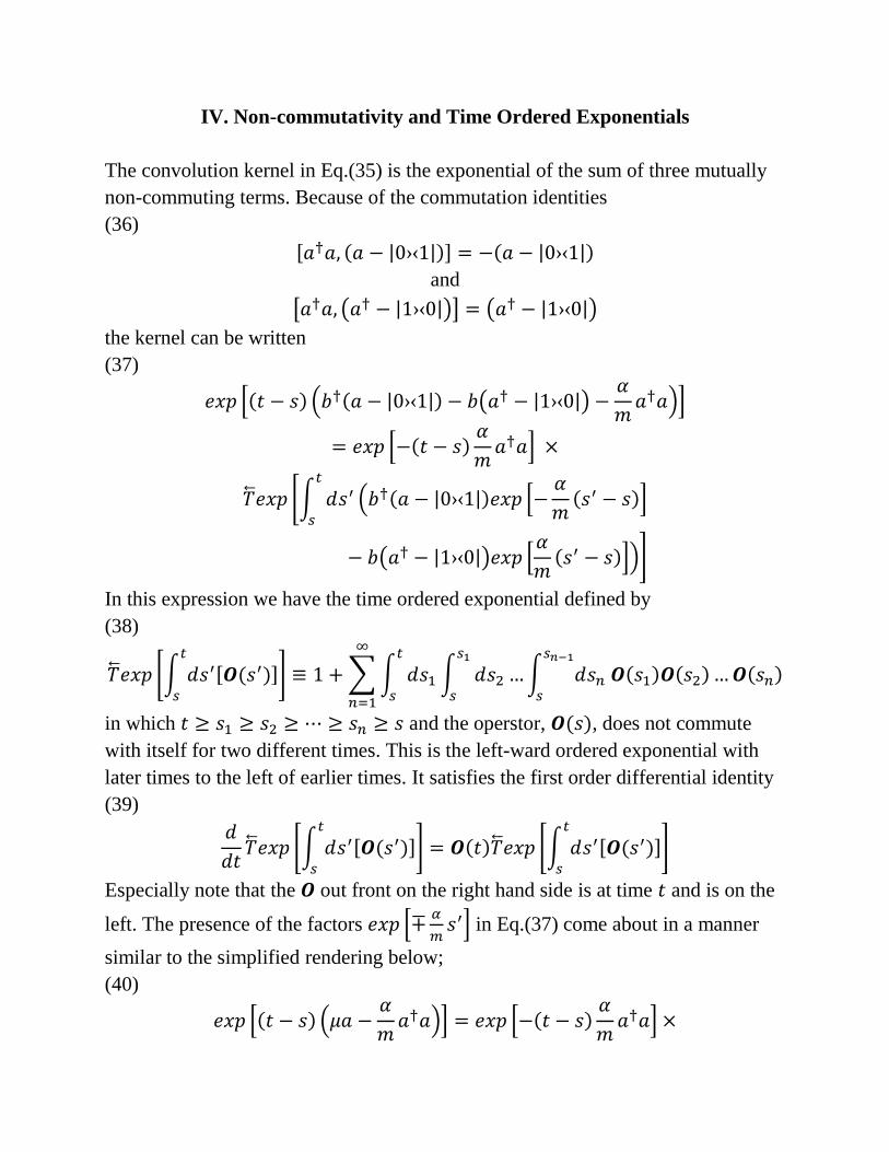
IV. Non-commutativity and Time Ordered Exponentials

The convolution kernel in Eq.(35) is the exponential of the sum of three mutually

non-commuting terms. Because of the commutation identities

(36)

and

the kernel can be written

(37)

In this expression we have the time ordered exponential defined by

(38)

in which and the operstor, , does not commute

with itself for two different times. This is the left-ward ordered exponential with

later times to the left of earlier times. It satisfies the first order differential identity

(39)

Especially note that the out front on the right hand side is at time and is on the

left. The presence of the factors

in Eq.(37) come about in a manner

similar to the simplified rendering below;

(40)

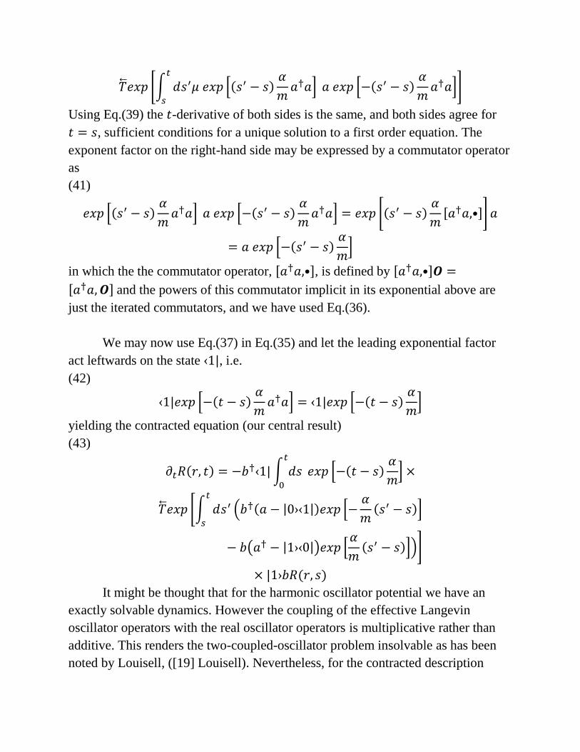
Using Eq.(39) the -derivative of both sides is the same, and both sides agree for

, sufficient conditions for a unique solution to a first order equation. The

exponent factor on the right-hand side may be expressed by a commutator operator

as

(41)

in which the the commutator operator, , is defined by

and the powers of this commutator implicit in its exponential above are

just the iterated commutators, and we have used Eq.(36).

We may now use Eq.(37) in Eq.(35) and let the leading exponential factor

act leftwards on the state , i.e.

(42)

yielding the contracted equation (our central result)

(43)

It might be thought that for the harmonic oscillator potential we have an

exactly solvable dynamics. However the coupling of the effective Langevin

oscillator operators with the real oscillator operators is multiplicative rather than

additive. This renders the two-coupled-oscillator problem insolvable as has been

noted by Louisell, ([19] Louisell). Nevertheless, for the contracted description

given here the oscillator case will be seen to be tractable and will later serve as a

check of the validity of the central result given in Eq.(43).

V. Elementary Checks of Eq.(43)

The minimal check is for the case =0. This makes (see Eq.(27).

Eq.(43) in turn becomes

(44)

If we expand the time ordered exponential according to the definition in Eq.(38)

the expectation values are non-zero for even order terms only, since they

must include equal amounts of and . That means the expectation

value of the time ordered exponential is an even order only power series in with

time dependent coefficients. The first few terms are (using Eq.(30) and Eq.(33))

(45)

The complexity of the terms in the series grows rapidly with the order of the term.

This results from the different orderings of equal amounts of and

. For example, in the above expression we have explicitly the second

and fourth order terms for . The corresponding coefficient for the sixth order

term (containing and an eight-fold time integral) works out to be

(46)

Consider calculating the moments of . Multiply Eq.(44) from the left by

and integrate by parts over . Because of the two factors of outside the time

ordered exponential, the result vanishes.

(47)

Consequently for all time. Choose the origin of coordinates to be .

Now do the same for . Only the in the time ordered exponential expansion

yields a non-zero result

(48)

This is precisely the same result obtained in the same way from Eq.(9). The

integral of this equation is the Ornstein-Furth equation ([16] Uhlenbeck and

Ornstein)

(49)

Using Eq.(9) we can also get and check it against the Gaussian moment

property that says

(50)

Eq.(9) implies

(51)

Note that the moments on the left and right hand sides are evaluated at time t.

Putting Eq.(49) into Eq.(51) verifies Eq.(50). This result also follows from Eq.(44)

although in a rather different way. Now we must keep the second term in the

expansion of Eq.(45).

(52)

wherein the last equality requires finishing the integrals. Note that appeared

part way through, at time and not at time .

One could proceed to calculate higher order moments by expanding the time

ordered exponential to higher order. However, since diffusion is a Gaussian

process the first two moments determine all higher order moments. From Eq.(49),

using to denote

, the distribution function for

is given by

(53)

However, this is a non-Markovian generalization of diffusion because of the non-

linear time dependence in .

VI. What it Means to be non-Markovian

The distribution function Eq.(53) is actually the conditional probability

distribution, given that the diffusing particle is initially at at time and is

distributed at at time . We write Eq.(53) given these conditions as the

two time conditional probability distribution ([20] Fox, [21] Wang and Uhlenbeck)

(54)

where

Note that

(55)

For Markovian diffusion, we have instead

. This is

valid for times

. For the non-Markovian diffusion, is a

nonlinear function of time whereas for the Markovian case it is a constant times

i.e. linear in time.

In the Markovian case , the Smoluchowski ([21] Wang and Uhlenbeck, note

II of the appendix), or Chapman-Kolmogorov ([22] Arnold, chapter 2), equation is

satisfied

(56)

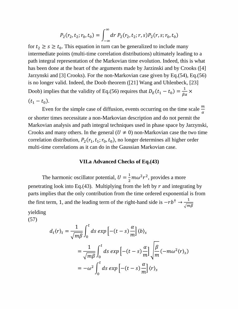
for . This equation in turn can be generalized to include many

intermediate points (multi-time correlation distributions) ultimately leading to a

path integral representation of the Markovian time evolution. Indeed, this is what

has been done at the heart of the arguments made by Jarzinski and by Crooks ([4]

Jarzynski and [3] Crooks). For the non-Markovian case given by Eq.(54), Eq.(56)

is no longer valid. Indeed, the Doob theorem ([21] Wang and Uhlenbeck, [23]

Doob) implies that the validity of Eq.(56) requires that

.

Even for the simple case of diffusion, events occurring on the time scale

or shorter times necessitate a non-Markovian description and do not permit the

Markovian analysis and path integral techniques used in phase space by Jarzynski,

Crooks and many others. In the general ( ) non-Markovian case the two time

correlation distribution, , no longer determines all higher order

multi-time correlations as it can do in the Gaussian Markovian case.

VII.a Advanced Checks of Eq.(43)

The harmonic oscillator potential,

, provides a more

penetrating look into Eq.(43). Multiplying from the left by and integrating by

parts implies that the only contribution from the time ordered exponential is from

the first term, , and the leading term of the right-hand side is

yielding

(57)

Therefore, by differentiation, we get the standard equation for a damped harmonic

oscillator

(58)

Much more difficult to obtain is the equation for . This is because

and times the time ordered exponential creates non-vanishing

terms from every order of the expansion of type Eq.(38). What we saw in Eq.(45)

and Eq.(46) for , becomes for the harmonic oscillator the even order terms

beginning with

(59)

The complexity increases rapidly with the order index, . The order of the time

variables is sequential for the first term only for each order. The variations are in

evidence for and for .What becomes clear upon further analysis is

that for even order , there is always a term

Moreover this is the only

term that does not contain consecutive ’s somewhere in the product and

consecutive ’s always come before consecutive ’s. The significance of these

facts is that a factor of from the left of the time ordered exponential will create

non-zero results for each

factor and for no others. That factors cannot

occur to the extreme left follows from the fact that they occur as

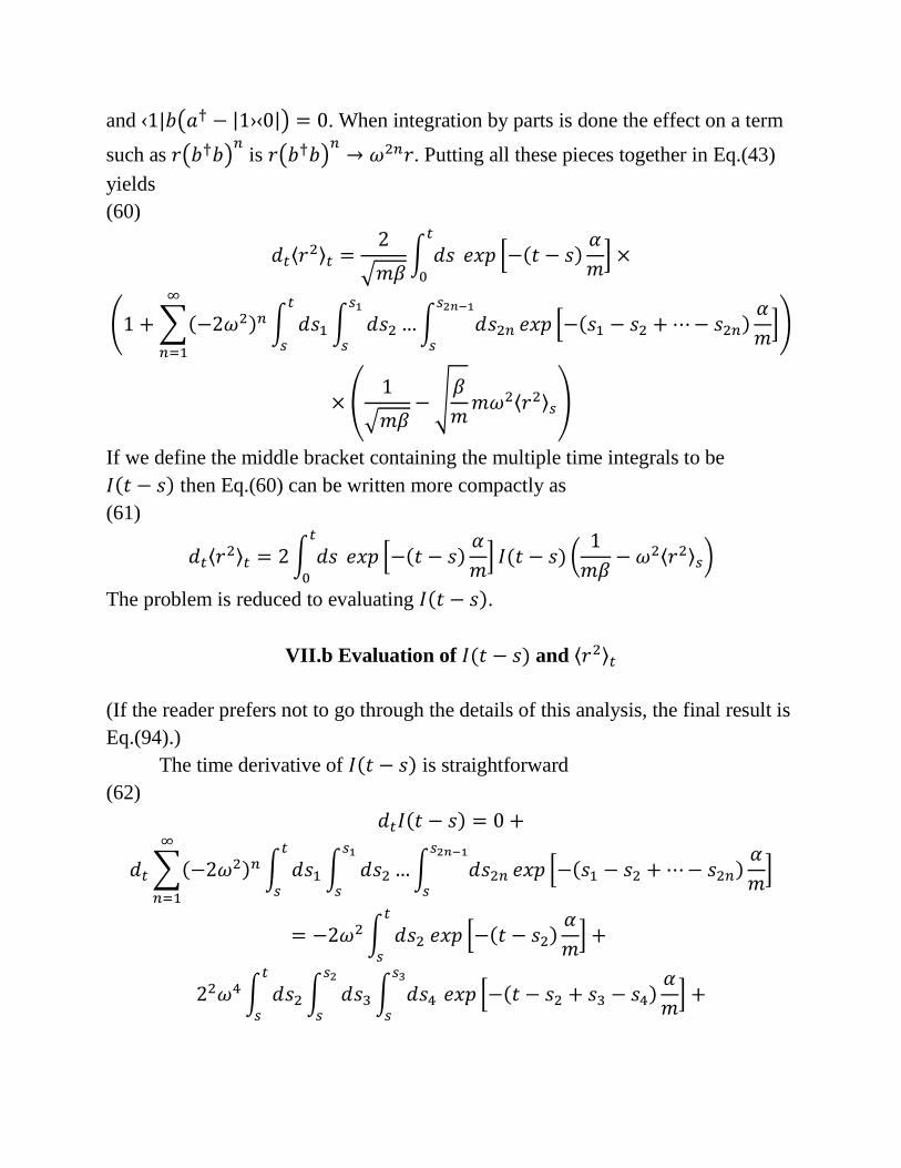
and . When integration by parts is done the effect on a term

such as

is . Putting all these pieces together in Eq.(43)

yields

(60)

If we define the middle bracket containing the multiple time integrals to be

then Eq.(60) can be written more compactly as

(61)

The problem is reduced to evaluating .

VII.b Evaluation of and

(If the reader prefers not to go through the details of this analysis, the final result is

Eq.(94).)

The time derivative of is straightforward

(62)

Note the new location for inside the exponential as well as in the upper limit of

the first integration. This leads to the equation and initial conditions

(63)

with

It is instructive to treat this second order equation in one variable as a first

order equation in two. Introduce

. and are dimensionless and

satisfies

with initial condition . Now write the

two variable equations in matrix form

(64)

Let the matrix be defined by

(65)

This matrix can be expressed in terms of the Pauli spin matrices

(66)

yielding

(67)

Using the initial conditions at , the solution to Eq.(64) is

(68)

because commutes with the other two Pauli matrices and can be factored out in

front. Any good introductory quantum mechanics book will have a justification of

the identity

(69)

Plugging this into Eq.(68) and reading off the upper component of the 2-vector

gives

(70)

This may be placed inside Eq.(61). The product in the kernel can be rendered as a

sum of exponentials

(71)

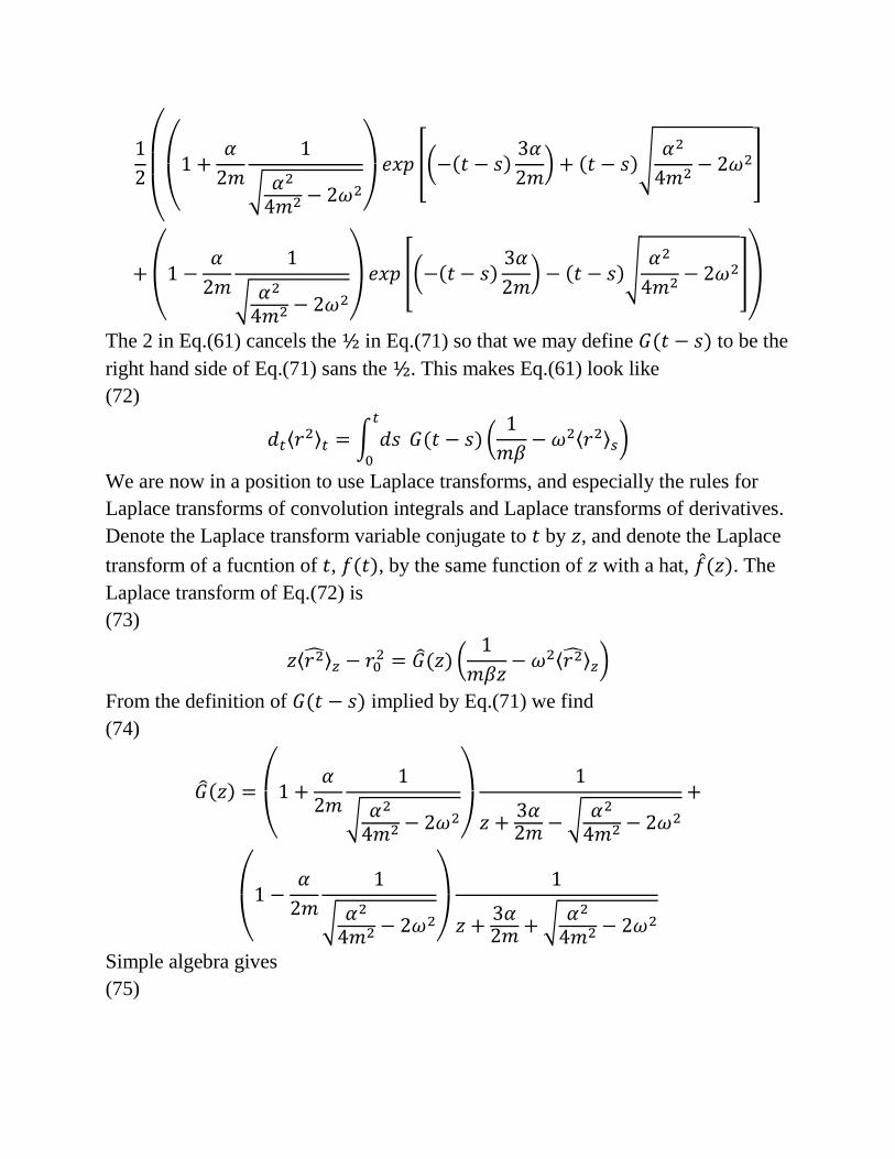
The 2 in Eq.(61) cancels the in Eq.(71) so that we may define to be the

right hand side of Eq.(71) sans the . This makes Eq.(61) look like

(72)

We are now in a position to use Laplace transforms, and especially the rules for

Laplace transforms of convolution integrals and Laplace transforms of derivatives.

Denote the Laplace transform variable conjugate to by , and denote the Laplace

transform of a fucntion of , , by the same function of with a hat, . The

Laplace transform of Eq.(72) is

(73)

From the definition of implied by Eq.(71) we find

(74)

Simple algebra gives

(75)

Define by

(76)

Therefore

(77)

and

(78)

where

and

Thus,

(79)

We must now take the Laplace transform inverse of this quantity.

Computing the Laplace inverse of the right hand side of Eq.(79) makes use

of several Laplace transform rules for and its Laplace transform :

(80)

Simple algebra verifies

(81)

The inverse Laplace transform of this quantity is

(82)

with the properties and . Using Eqs.(79-82), we get

(83)

Although involving algebra only, the reduction of this expression takes quite a lot

of manipulation. Begin with

(84)

From Eq.(78) it follows that

(85)

and

Putting this into Eq.(84) and then that result into Eq.(83) yields

(86)

Now note that

(87)

and define by

(88)

Eq.(86) becomes

(89)

The terms inside can be simplified using the identity

(90)

Therefore we get

(91)

Finally, putting everything together, we get

(92)

One more observation puts this formula into its final form

(93)

Therefore,

(94)

and agrees with ([15] Chandrasekhar, Eq.(217)).

VIII. Non-Markovian Distribution for the Harmonic Oscillator

Return to Eqs.(57-58) to see how the first moment of evolves in time. The

initial conditions for Eq.(58) are and (see Eq.(57)). The

solution is

(95)

Introduce the short-hand notation

(96)

so that we can write

(97)

and

Clearly and yielding the equipartition of energy result for

. The variance,

, is equal to

(98)

Because we have a Gaussian process we can immediately write down the

conditional probability distribution

(99)

This is manifestly non-Markovian because of the dependence of . Note the

two limits

(100)

and

where is the normalized Boltzmann distribution for the potential energy

. In the Gaussian Markovian case, the distribution could be

used to construct all multi-time correlation functions ([21] Wang and Uhlenbeck,

[11] Fox), but not in the non-Markovian case that we have here.

IX. Non-equilibrium Thermodynamics

Instead of considering phase space trajectories and their time reversed

partners, we have contracted the description and derived the time evolution in

coordinate space. Time reversed phase space trajectories require the ability to

reverse each and every particle momentum simultaneously and instantaneously.

While this is possible in a molecular dynamics computation on a computer it is

impossible in real experiments, and will always remain so. Alternatively we may

ask if thermodynamic ideas can be extended into the non-equilibrium regime. For

thermostated systems this means we should look at the Helmholtz free energy, ,

that attains a minium value in equilibrium.

We will see that in the “over-damped” case ( ) the Helmholtz free

energy for a harmonic oscillator decreases monotonically in time. In the under-

damped case ( ) monotonicity is broken and the Helmholtz free

energy shows damped oscillations as it approaches its equilibrium value. The

Helmholtz free energy is defined by

(101)

in which is the internal energy defined by

(102)

and is the entropy defined by

(103)

where is the Kelvin temperature, is Boltzmann’s constant and the logarithm

term could have a constant included to make its argument appropriately

dimensionless but this would not show up in the time derivative and is, therefore,

omitted. The time derivative of is

(104)

in which we have dropped the term

(105)

Eq.(105) follows from Eq.(44) because here is there and the

right hand side of Eq.(44) begins with which upon integration by parts

vanishes since vanishes at the boundaries. In general, the non-Markovian nature

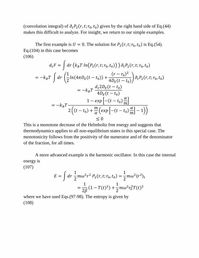
(convolution integral) of given by the right hand side of Eq.(44)

makes this difficult to analyze. For insight, we return to our simple examples.

The first example is . The solution for is Eq.(54).

Eq.(104) in this case becomes

(106)

This is a monotone decrease of the Helmholtz free energy and suggests that

thermodynamics applies to all non-equilibrium states in this special case. The

monotonicity follows from the positivity of the numerator and of the denominator

of the fraction, for all times.

A more advanced example is the harmonic oscillator. In this case the internal

energy is

(107)

where we have used Eqs.(97-98). The entropy is given by

(108)

Thus, for the harmonic oscillator,

(109)

Therefore, the time derivative is

(110)

where is defined in Eq.(96). The factor was introduced in Eq.(88) and is

real in the overdamped case, and is imaginary in the underdamped case. Consider

the real case first. Introduce the parameter

. Overdamped case means

and underdamped case means .We can rewrite in the form

(111)

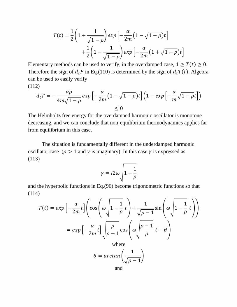
Elementary methods can be used to verify, in the overdamped case, .

Therefore the sign of in Eq.(110) is determined by the sign of . Algebra

can be used to easily verify

(112)

The Helmholtz free energy for the overdamped harmonic oscillator is monotone

decreasing, and we can conclude that non-equilibrium thermodynamics applies far

from equilibrium in this case.

The situation is fundamentally different in the underdamped harmonic

oscillator case ( and is imaginary). In this case is expressed as

(113)

and the hyperbolic functions in Eq.(96) become trigonometric functions so that

(114)

where

and

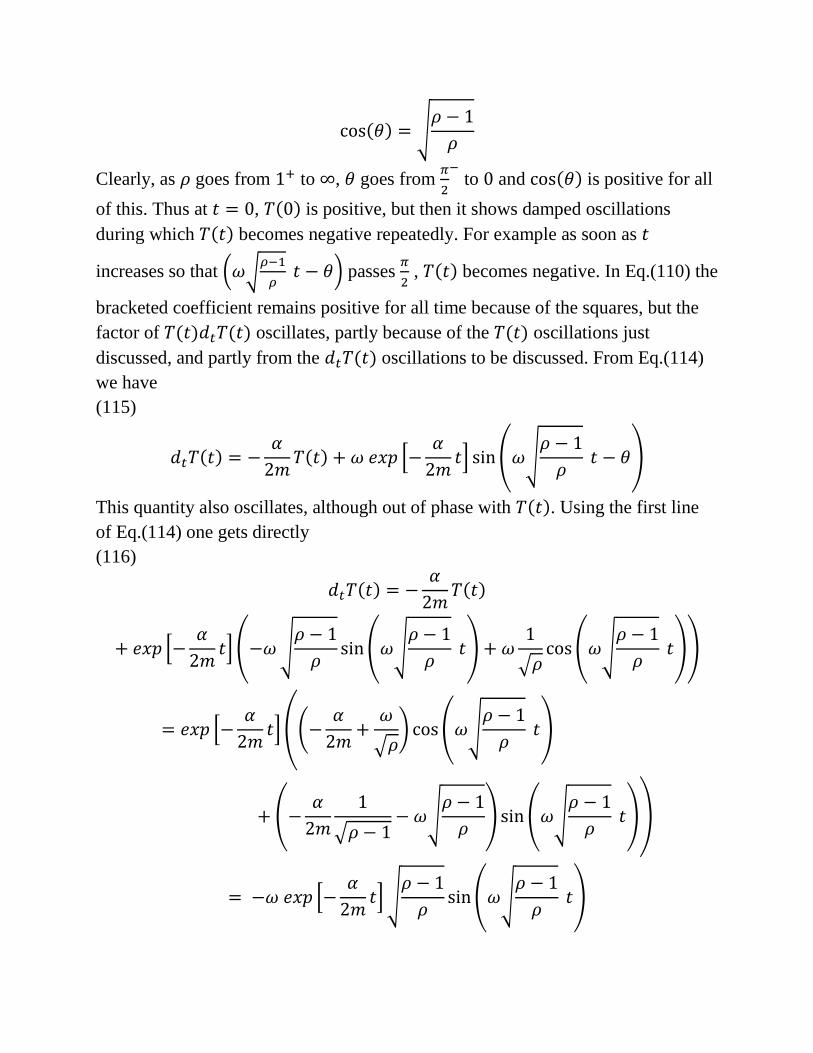
Clearly, as goes from to , goes from

to and is positive for all

of this. Thus at , is positive, but then it shows damped oscillations

during which becomes negative repeatedly. For example as soon as

increases so that

passes

, becomes negative. In Eq.(110) the

bracketed coefficient remains positive for all time because of the squares, but the

factor of oscillates, partly because of the oscillations just

discussed, and partly from the oscillations to be discussed. From Eq.(114)

we have

(115)

This quantity also oscillates, although out of phase with . Using the first line

of Eq.(114) one gets directly

(116)

The sign of the product is determined by the sign of

(117)

Note that the second term of the last line is positive for all . Only the first

term can change the sign and this happens when the first term is more negative

than the second term is positive. As it turns out, there is always a finite range of

values of for which can make the expression in Eq.(117) negative for any .

To see this note initially that if is very much greater than then the first term

dominates and periodically changes sign. The issue is whether this is possible for

. Look at the first line of Eq.(117) and assume

for large .

Changes of sign in Eq.(117) occur when (assuming

does not vanish

at the same time, a verifiably safe assumption).

(118)

This is equivalent with

(119)

which happens periodically in . The amount of the axis for which the expression

in Eq.(117) is negative decreases as gets large. Negative values correspond with

increases of the Helmholtz free energy. Therfore, in the case of the underdamped

harmonic oscillator the generalization of thermodynamics to the non-equilibrium

states fails because is no longer monotonically decreasing.

X. Underdamping in Sub-cellular Biology

Generally the molecular events occurring in sub-cellular biology are

overdamped. An example is the elasticity of the neck linker of the kinesin

molecule the attaches to the kinesin head and plays a central role in the kinesin

mechanism ([8] Fox, chapter 4). The harmonic oscillator approach to the neck

linker elasticity results in an extreme overdamped value. Not only is non-

equilibrium thermodynamics reasonable for this regime, it is possible to

approximate the dynamics by a Markovian dynamics for which the path integral

techniques of Jarzinski and Crooks are valid (although here we are in coordinate

space only, not full phase space).

The Markovian approximation to Eq.(43) can be justified with various

degrees of rigor. Here, we will see how it comes about using the Dirac delta

function because this approach is very transparent. Suppose you have the equation

(120)

If is large, write this equation in the form

(121)

and contemplate the limit . Because

(122)

we can write

(123)

where the factor of ½ arises from the end point rule for delta function integrals, i.e.

is in the delta function and is the upper limit of integration. Thus, for large

enough it follows that

(124)

If we apply this result to Eq.(43), we see that the limits of integration inside the

time ordered exponential become the same, i.e. so that the time ordered

exponential simply becomes . Thus the Markovian approximation to Eq.(43) is

(125)

wherein we have used Eq.(27) for general potential energy , and the constant in

front of the right hand side is Einstein’s formula for the diffusion constant.

Eq.(125) may be recognized as diffusion in a potential and is sometimes called the

Smoluchowski equation ([15] Chandrasekhar, pp. 40-41). Because the Markov

approximation requires that is large (the relaxation time is very short) this

approximation only holds for the overdamped case.

Using the last line of Eq.(9) we can show that the Helmholtz free energy

given by analogs of Eqs.(101-103) satisfies

(126)

The third line follows from integration by parts and the vanishing of on the

boundary. Thus a non-equilibrium thermodynamics is valid for all non-equilibrium

states in the Markov approximation and the Helmholtz free energy decreases

monotonically in an undriven thermostated system. This situation in no longer

valid in the full non-Markovian picture (Eq.(43)) as we saw for the underdamped

harmonic oscillator and as would be true for underdamped motion in a general

potential.

Underdamped motion in sub-cellular biology is rarely documented because

this realm is seriously overdamped in most situations. In the example of kinesin

referred to earlier the elasticity time scale was found to be nanoseconds, whereas

the damping time scale was picoseconds. This means the kinesin dynamics is very

overdamped. Recently there have been claims that some protein-ligand interactions

are indeed underdamped ([24] Turton et al.). In these studies the elasticity time

scale is picoseconds and because the proteins fragments of the type studied are

much larger than the kinesin heads the relaxation time scale is much less than

picoseconds. These circumstances make the system underdamped and, therefore,

non-Markovian. I quote from the abstract of Turton et al.:

“Low-frequency collective vibrational modes in proteins have been proposed as being

responsible for efficiently directing biochemical reactions and biological energy transport.

However, evidence of the existence of delocalized vibrational modes is scarce and proof of their

involvement in biological function absent. Here we apply extremely sensitive femtosecond

optical Kerr-effect spectroscopy to study the depolarized Raman spectra of lysozyme and its

complex with the inhibitor triacetylchitotriose in solution. Underdamped delocalized vibrational

modes in the terahertz frequency domain are identified and shown to blue-shift and strengthen

upon inhibitor binding. This demonstrates that the ligand-binding coordinate in proteins is

underdamped and not simply solvent-controlled as previously assumed. The presence of such

underdamped delocalized modes in proteins may have significant implications for the

understanding of the efficiency of ligand binding and protein–molecule interactions, and has

wider implications for biochemical reactivity and biological function.”

Thus the significance of underdamped motion in sub-cellular biology may grow in

the future. Its description is intrinsically non-Markovian and not controlled by

thermodynamic rules. In particular the Helmholtz free energy does not decrease

monotonically. Perhaps the content of this paper will help in the application of

physically realistic methods to the understanding of thermostated systems in nano-

biology and in nano-technology.

References

[1] D. J. Evans, E. G. D. Cohen and G. P. Morriss, Physical Review Letters, 71,

2401, (1993).

[2] G. Gallavotti and E. G. D. Cohen, Physical Review Letters, 74, 2694, (1995).

[3] G. Crooks, Physical Review E 60, 2721, (1999).

[4] C. Jarzynski, Physical Review Letters, 78, 2690, (1997).

[5] J. Gore, F. Ritort and C. Bustamante, Proceedings of the National Academy of

Sciences, 100 (22), 12564, (2003).

[6] W. G. Hoover and C. G. Hoover, arXiv submit/0232492, 16 April (2011).

[7] J. England, The Journal of Chemical Physics, 139, 121923, (2013).

[8] R. F. Fox, Nanotech 2004, 3, 18, (2004); Rectified Brownian Motion, an eBook,

http://www.fefox.com/ARTICLES/RectifiedBrownianMotioneBook.pdf.

[9] J. L. Davis and R. F. Fox, Journal of Statistical Physics, 22, 627, (1980).

[10] R. Spinney and I. Ford, arXiv:1201.6381v1, 30 Jan (2012).

[11] R. F. Fox, Physics Reports, 48 (3), 179, (1978).

[12] G. E. Uhlenbeck and G. W. Ford, Lectures in Statistical Mechanics (American

Mathematical Society, Providence, R.I., 1963).

[13] R. F. Fox and G. E. Uhlenbeck, Physics of Fluids, 13, 1893, (1970); 13, 2881,

(1970).

[14] J. E. Keizer, Statistical Thermodynamics of Nonequilibrium Processes

(Springer-Verlag, New York, 1987).

[15] S. Chandrasekhar, Reviews of Modern Physics, 15 (1), 1, (1943), pp. 31-42.

[16] G. E. Uhlenbeck and L. S. Ornstein, Physical Review, 36, 823 (1930), p. 826.

[17] R. Zwanzig, Physical Review, 124, 983, (1961).

[18] H. Mori, Progress in Theoretical Physics, 33, 423, (1965).

[19] W. H. Louisell, Quantum Statistical Properties of Radiation, (John Wiley and

Sons, New York, 1973), pp. 418-420.

[20] R. F. Fox, Physics Reports, 48 (3), 179, (1978), section I.3.

[21] M. C. Wang and G. E. Uhlenbeck, Reviews of Modern Physics, 17, 323

(1945).

[22] L. Arnold, Stochastic Differential Equations, (John Wiley and Sons, New

York, 1974)

[23] J. L. Doob, Annals of Mathematics, 43, 351 (1942).

[24] D. A. Turton, H. M. Senn, T. Harwood, A.J. Laphorn, E. M. Ellis and K.

Wynne, Nature Communications, DOI 10.1038/ncomms4999, (2014).

17 September 2014

Ronald F. Fox

Smyrna, Georgia