contributor the story of factor-based investing€¦ · · 2017-02-01the story of factor-based...

RESEARCH

Smart Beta

CONTRIBUTOR

Sunjiv Mainie, CFA, CQF

Senior Director and Head of

Research & Design (EMEA)

[email protected]

The Story of Factor-Based

Investing

1.0 INTRODUCTION

For decades, investment portfolios were constructed from a combination of

market cap weighted index funds and active funds. Cap weighted index

funds can provide a basis for investors to acquire the market portfolio in a

simple, transparent, and cost-effective manner. By contrast, active funds

promise potentially higher returns, albeit at the cost of greater complexity

and higher fees.

In recent years, institutional investors have employed a new approach to

portfolio construction: factor-based investing.1 This increasingly popular

approach lies between passive and active investing, allowing investors to

target specific risk factors (return drivers) as well as market beta. These

strategies use a transparent, systematic, rules-based method at relatively

low costs. This enables investors to implement active strategies while

remaining under the passive umbrella.

In this paper, the origins and evolution of factor-based investing are

examined. The theories underpinning factor-based investing, developed

from the Capital Asset Pricing Model (CAPM),2 and its multifactor

extensions are discussed. The economic intuition behind factor

performance is analyzed, along with its implementation. Finally, likely

innovations and future product strategies are briefly considered.

1 Betas measure exposures to a given factor. One invests in factors, not betas. Therefore, terms such as alternate beta and smart beta will

not be used in this paper.

2 Over the years, CAPM has had its critics. Numerous research studies have documented the inefficiencies of the simple single factor approach. However, the basic intuition behind CAPM holds true—that factors’ underlying assets determine asset risk premia, and these risk premia provide compensation for investors bearing systematic risk.

In recent years, institutional investors have employed a new approach to portfolio construction: factor-based investing.

mailto:[email protected]

The Story of Factor-Based Investing February 2015

RESEARCH | Smart Beta 2

2.0 FACTOR THEORY

Factor risks are the driving force of assets’ risk premia. One of the first

financial theories to model asset returns as a function of factor risks was

the linear CAPM. This model was formulated in the 1960s and stated that

there is only one factor, the market factor, driving the returns of assets.

Moreover, the CAPM stipulates that the return of an asset is the sum of

systematic return and specific return, as shown in equation one.

𝑟𝑖 = 𝑟𝑓 + 𝛽𝑖 (𝑟𝑀 − 𝑟𝑓) + 𝜀𝑖

Equation 1

where:

𝑟𝑖 = return for asset 𝑖

𝑟𝑓 = risk-free rate

𝛽𝑖 = beta for asset 𝑖

𝑟𝑀 = market factor return

𝜀𝑖 = asset 𝑖 specific return

The CAPM models the systematic return as a function of the beta that

measures the sensitivity of assets’ returns to the market return. An asset’s

beta is given by:

𝜷𝒊 = 𝝆𝒊,𝑴 𝝈𝒊

𝝈𝑴

Equation 2

where:

𝝆𝒊,𝑴 = the correlation coefficient between asset 𝒊 and the market

𝝈𝒊 = the volatility of asset 𝒊

𝝈𝑴 = the volatility of the market

Note that the last term in Equation 1, the specific return component, is

modeled as a normal random variable with a mean of zero - 𝜺𝒊 ~𝑵(𝟎, 𝜽𝒊𝟐).

Therefore, the specific risk of asset 𝒊 is 𝜽𝒊.

This model was formulated in the 1960s and stated that there is only one factor, the market factor, driving the returns of assets.



The CAPM assumes that for an individual asset, the systematic return and

the specific return are independent of each other (uncorrelated). Moreover,

if the specific returns of different assets are also assumed to be

independent of each other, then it can be shown that a portfolio holding N

assets will have variance defined as:

𝝈𝒑𝟐 = 𝜷𝒑

𝟐𝝈𝑴𝟐 + ∑ 𝒘𝒊

𝟐𝜽𝒊𝟐𝑵

𝒊=𝟏

Equation 3

where:

𝝈𝒑 = portfolio volatility

𝜷𝒑 = portfolio beta

𝒘𝒊 = asset weight 𝒊

Equation 3 highlights two sources of risk within any portfolio, one

systematic and the other specific. This has important implications for

portfolio construction. First, the specific component may be diversified

away by holding many assets. For example, an equal-weighted portfolio

holding N assets, all with the same specific risk, would result in a portfolio

specific risk of 𝜽

√𝑵. As the number of assets N increases, the specific risk

decreases. Second, the systematic risk is a function of the portfolio beta

and market risk. Therefore, a traditional, long-only portfolio holding many

assets would have most of its risk exposed to the market.

This analysis views the CAPM as a possible risk tool. However, this model

was originally developed as an equilibrium pricing model, where its function

was to provide return expectations of individual assets. Therefore, in terms

of pricing, it can be rewritten as:

𝔼(𝒓𝒊 − 𝒓𝒇) = 𝜷𝒊[𝔼(𝒓𝑴) − 𝒓𝒇]

Equation 4

Note that the specific term has been dropped.3 Equation 4 reveals valuable

insight into the mechanics of investment performance, namely that

expected returns of assets are proportional to their systematic risks, as

measured by their betas. On the other hand, specific risks may be

diversified away and are not rewarded with excess returns.

The discovery of the subtle differences between how the CAPM can be

used, whether in risk or expectation, provided the foundation for many of

the risk and alpha models that followed. The 1970s saw the incorporation

of more factors (beyond just the market factor) to improve the CAPM as a

risk tool. The first multi-factor model was developed by Stephen Ross in

3 The expectation of the specific term, which is modeled as a normal random variable with a mean of zero, is zero.

A traditional, long-only portfolio holding many assets would have most of its risk exposed to the market.



1976. Many of today’s commercial risk models are based on his Arbitrage

Pricing Theory (APT) including macroeconomic factor models, fundamental

factor models, and statistical factor models.

Moreover, pricing anomalies4 were soon discovered that contradicted the

CAPM and its use as a pricing model. The Fama-French Three-Factor

Equity Model, incorporating the size and value effects in addition to the

market, was widely regarded as an improvement (Fama and French,

1993).5 An extension of this three-factor model is the Carhart four-factor

model, where the momentum effect is included (Carhart, 2012).6 From a

practitioner’s point of view, this highlights that there may be other priced

factors, in addition to the market, that could reward investors over time.

This can be written as:

𝔼(𝒓𝒊 − 𝒓𝒇) = 𝜷𝒊,𝟏𝔼(𝒇𝟏) + 𝜷𝒊,𝟐𝔼(𝒇𝟐) + ⋯ + 𝜷𝒊,𝑲𝔼(𝒇𝑲)

Equation 5

where:

𝜷𝒊,𝒌= beta for asset 𝒊 with respect to factor 𝒌

𝔼(𝒇𝒌) = the risk premium of factor 𝒌

These factors drive the performance of investment portfolios. They

underpin many of the factor-based products currently available in the

market.7

3.0 EQUITY FACTORS

3.1 Value

The benefits of value investing have been known since the 1930s. Its

strongest advocates were Benjamin Graham and, more recently, Warren

Buffet. Considerable academic research documents the value effect. Most

agree that value stocks provide above-market returns. However, there is

no single consensus as to why this is the case, and explanations fall

broadly into two camps: the rational and the behavioral.

Rational theories explain how the value premium arises from investors

requiring compensation for bearing higher systemic risk in the form of

financial distress (Fama and French 1996). For example, in recessionary

environments, value firms (like manufacturing) find it difficult to shift their

4 Within this paper, the terms “factors” and “anomalies” are used interchangeably.

5 The small-cap effect is the difference between the return on a portfolio of small stocks and the return on a portfolio of large stocks. The value effect is the difference between the return on a portfolio of high-book-to-market stocks and the return on a portfolio of low-book-to-market stocks.

6 The momentum effect is the difference between the return on a portfolio of high-performing stocks and the return on a portfolio of low-performing stocks.

7 For further details on Factor Theory see Qian et al, 2007.

Behavioral theories argue that the value risk premium might be driven by investors incorrectly extrapolating the past earnings growth rates of companies.



activities to more profitable ones. By contrast, growth firms (such as

technology) can disinvest relatively easily, as a large proportion of their

capital is human capital. Hence, value firms are perceived as being riskier

than their growth counterparts and, as such, should command a premium.

Behavioral theories argue that the value risk premium might be driven by

investors incorrectly extrapolating the past earnings growth rates of

companies (Lakonishok et al 1994). High profile, glamorous stocks that

have high valuations are bought by naïve investors expecting continued

high growth rates in earnings. This pushes up their prices and, as a

consequence, lowers their rates of return. At the same time, value stocks

are cheap, as investors underestimate their future growth rates. Their

cheapness does not arise from the fact that they are fundamentally riskier.

There are many ways to define value. For example, cash-flow yield and

earnings yield examine cheapness while emphasizing profitability.

Dividend yield provides insight into management’s assessment of future

profitability. Using the balance sheet item of net assets (book) gives a

measure of liquidation value. Other value measures include predicted

earnings yield and EBITDA8-to-enterprise value. Equity products that aim

to harvest the value premium can be constructed by using one or a

combination of these measures.9

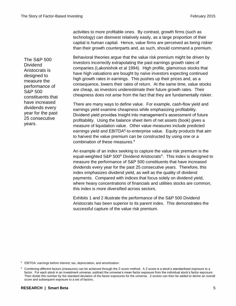
An example of an index seeking to capture the value risk premium is the

equal-weighted S&P 500® Dividend Aristocrats®. This index is designed to

measure the performance of S&P 500 constituents that have increased

dividends every year for the past 25 consecutive years. Therefore, this

index emphasizes dividend yield, as well as the quality of dividend

payments. Compared with indices that focus solely on dividend yield,

where heavy concentrations of financials and utilities stocks are common,

this index is more diversified across sectors.

Exhibits 1 and 2 illustrate the performance of the S&P 500 Dividend

Aristocrats has been superior to its parent index. This demonstrates the

successful capture of the value risk premium.

8 EBITDA: earnings before interest, tax, depreciation, and amortization.

9 Combining different factors (measures) can be achieved through the Z-score method. A Z-score is a stock’s standardized exposure to a factor. For each stock in an investment universe, subtract the universe’s mean factor exposure from the individual stock’s factor exposure. Then divide this number by the standard deviation of the factor exposures for the universe. Z-scores can then be added to derive an overall score and subsequent exposure to a set of factors.

The S&P 500 Dividend Aristocrats is designed to measure the performance of S&P 500 constituents that have increased dividends every year for the past 25 consecutive years.



Exhibit 1: The S&P 500 Dividend Aristocrats Versus the S&P 500

Source: S&P Dow Jones Indices LLC. Data from Jan. 31, 1990, to Oct. 31, 2014. Past performance is no guarantee of future results. Charts and tables are provided for illustrative purposes and may reflect hypothetical historical performance. Please see the Performance Disclosures at the end of this document for more information regarding the inherent limitations associated with back-tested performance.

Exhibit 2: S&P 500 Dividend Aristocrats and S&P 500 Performance Comparison

INDEX ANNUALIZED RETURN (%)

ANNUALIZED RISK (%)

RISK-ADJUSTED RETURN

S&P 500 Dividend Aristocrats

12.4 13.6 0.91

S&P 500 9.9 14.6 0.68


3.2 Momentum

The first major academic study of momentum was by Jegadeesh and

Titman (1993). They document price momentum as an investment factor

where recent winners continue to win and losers continue to lose. Price

momentum is observed in many asset classes including commodities,

government and corporate bonds, and industries. Commodity Trading

Advisor funds (CTAs) have successfully pursued these strategies since the

1980s.

Momentum arises because of the biased way that investors interpret or act

on information. Explanations of the price momentum effect are

predominantly behavioral and fall on two sides: overreaction and

underreaction. Daniel et al (2001) argue that some investors are

overconfident and overestimate their abilities to forecast firms’ future cash

flows. Based on this overconfidence, they overreact, pushing up the prices

of stocks and generating momentum. Hong et al (2000) show that the slow

diffusion of information into prices causes an initial underreaction; investors

then learn about the quality of this information, which pushes prices up

further.

0

200

400

600

800

1000

1200

1400

1600

1800

2000

1990

1991

1992

1993

1994

1995

1996

1997

1998

1999

2000

2001

2002

2003

2004

2005

2006

2007

2008

2009

2010

2011

2012

2013

2014

S&P 500 Dividend Aristocrats S&P 500

Price momentum is observed in many asset classes including commodities, government and corporate bonds, and industries.



Other theories point to the imperfect information available to all investors

and to imperfect market structure. Imperfect information refers to the

agency problem, wherein management has strong incentives to promote

good news and hide bad news. Institutional fund managers can arbitrage

good news, but the vast majority are unable to exploit bad news due to

short-selling constraints of what is, in practice, an imperfect market

structure.

Typical measures of price momentum may involve one or a combination of

the following: one-month reversals, six-month return, and twelve-month

return. Some practitioners risk adjust performance returns too. More

complicated measures include moving averages, relative strength index

(RSI), and Bollinger bands.

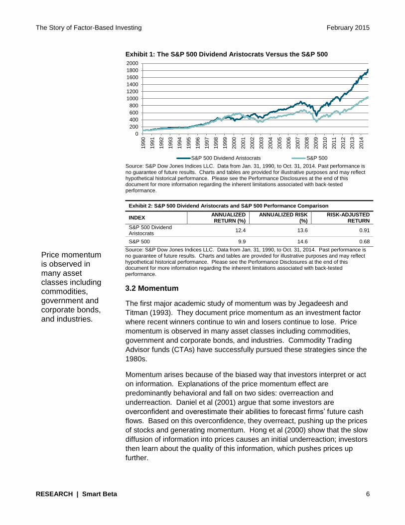
The S&P Europe 350® Momentum Index seeks to capture the momentum

anomaly. This index is based on price momentum, combining one-month

reversals and twelve-month returns, and it is adjusted for volatility. The

final Z-score combinations are ranked, and the top quintile is selected for

inclusion in the index. Constituent weights are determined by a simple

transformation—score multiplied by float-adjusted market capitalization.

Exhibit 3: The S&P Europe 350 Momentum Index Versus the S&P Europe 350

Source: S&P Dow Jones Indices LLC. Data from April 30, 2001, to Oct. 31, 2014. Past performance is no guarantee of future results. Charts and tables are provided for illustrative purposes and may reflect hypothetical historical performance. Please see the Performance Disclosures at the end of this document for more information regarding the inherent limitations associated with back-tested performance.

Exhibit 4: S&P Europe 350 Momentum Index and S&P Europe 350 Performance Comparison


ANNUALIZED RISK (%)


S&P Europe 350 Momentum Index

6.1 14.3 0.43

S&P Europe 350 2.9 15.6 0.19

Source: S&P Dow Jones Indices LLC. Data from April 30, 2001, to Oct. 31, 2014. Past performance is no guarantee of future results. Charts and tables are provided for illustrative purposes and may reflect hypothetical historical performance. Please see the Performance Disclosures at the end of this document for more information regarding the inherent limitations associated with back-tested performance.

0

50

100

150

200

250

S&P Europe 350 Momentum Index S&P Europe 350

Constituent weights are determined by a simple transformation—score multiplied by float-adjusted market capitalization.



Over the period, targeting the momentum factor increases the risk-adjusted

return.

3.3 Quality

In contrast to momentum factors embedded in behavioral bias, investing

based on quality factors is more fundamental in approach. Investors

endeavor to ascertain the health of a firm’s business and the competence

of its management. Quality factors attempt to identify firms that generate

abnormal profits from their competitive operations. Moreover, management

delivers these profits directly to shareholders, without succumbing to the

agency problem.

In practice, fund managers use a combination of measures as a proxy for

quality, such as gross profit margin, quick ratio, and total asset turnover

ratio. However, a robust combination should target three key company

attributes: profitability (competitiveness), earnings quality (agency problem),

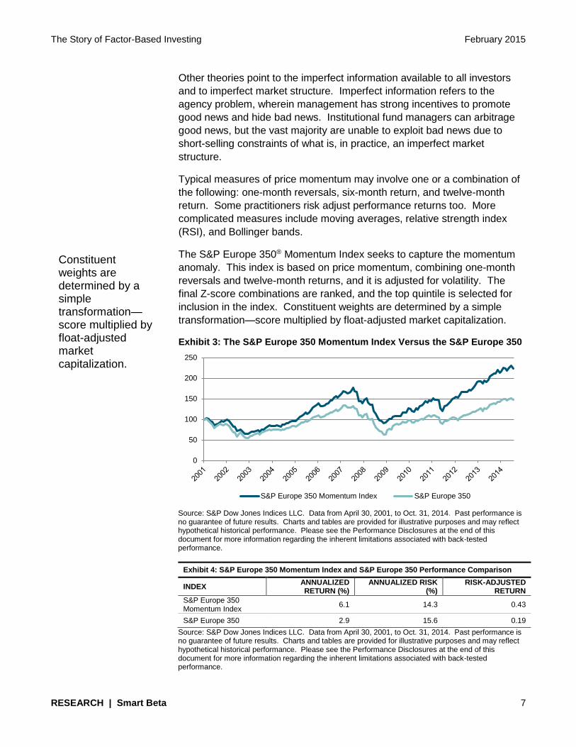
and capital structure (financial risk). The S&P 500 Quality Index combines

return on equity, the accruals ratio, and financial leverage, respectively.10

These items require information from all financial statements. This index

selects the top 100 stocks with the highest quality scores. Weights are

computed as the product of the overall quality score and the float-adjusted

market capitalization.

Exhibits 5 and 6 show the successful capture of the quality risk premium

over the analyzed period.

Exhibit 5: The S&P 500 Quality Index Versus the S&P 500

Source: S&P Dow Jones Indices LLC. Data from Dec. 31, 1994, to Oct. 31, 2014. Past performance is no guarantee of future results. Charts and tables are provided for illustrative purposes and may reflect hypothetical historical performance. Please see the Performance Disclosures at the end of this document for more information regarding the inherent limitations associated with back-tested performance.

10 Return on equity is calculated by dividing a company’s trailing, 12-month earnings-per-share by the company’s latest book-value-per-share.

The accruals ratio is the change in net operating assets over the past year divided by the company’s average net assets over the past two years. Financial leverage is computed by taking the latest total debt figures available and dividing this by the company’s book value. Note: these are combined using the Z-score method.

0

200

400

600

800

1000

1200

1400

1600

S&P 500 Quality Index S&P 500

The S&P 500 Quality Index combines return on equity, the accruals ratio, and financial leverage, respectively.



Exhibit 6: S&P 500 Quality Index and S&P 500 Performance Comparison


ANNUALIZED RISK (%)


S&P 500 Quality Index 14.1 14.0 1.01

S&P 500 9.8 15.2 0.64


3.4 Size

The market capitalization of a company (its size) has long been a popular

investment factor. Considerable research points to the outperformance of

small-cap stocks relative to large-cap stocks over the long run.

Explanations for this anomaly include the fact that investors require an

additional risk premium, as small-cap stocks are less established and

therefore more risky than large-cap stocks, small-cap stocks receive

relatively less analyst coverage resulting in more mispriced opportunities,

and investors require additional compensation for stocks that are not

household names.

The size effect does have its critics. Since the mid-1980s, small-cap stocks

have done better than large-cap stocks (in general). However, after

adjusting for market exposure, the size effect quickly disappears (Dimson

et al 2011). Therefore, arguably, the size effect should no longer be

included in the Fama-French Three-Factor Model.

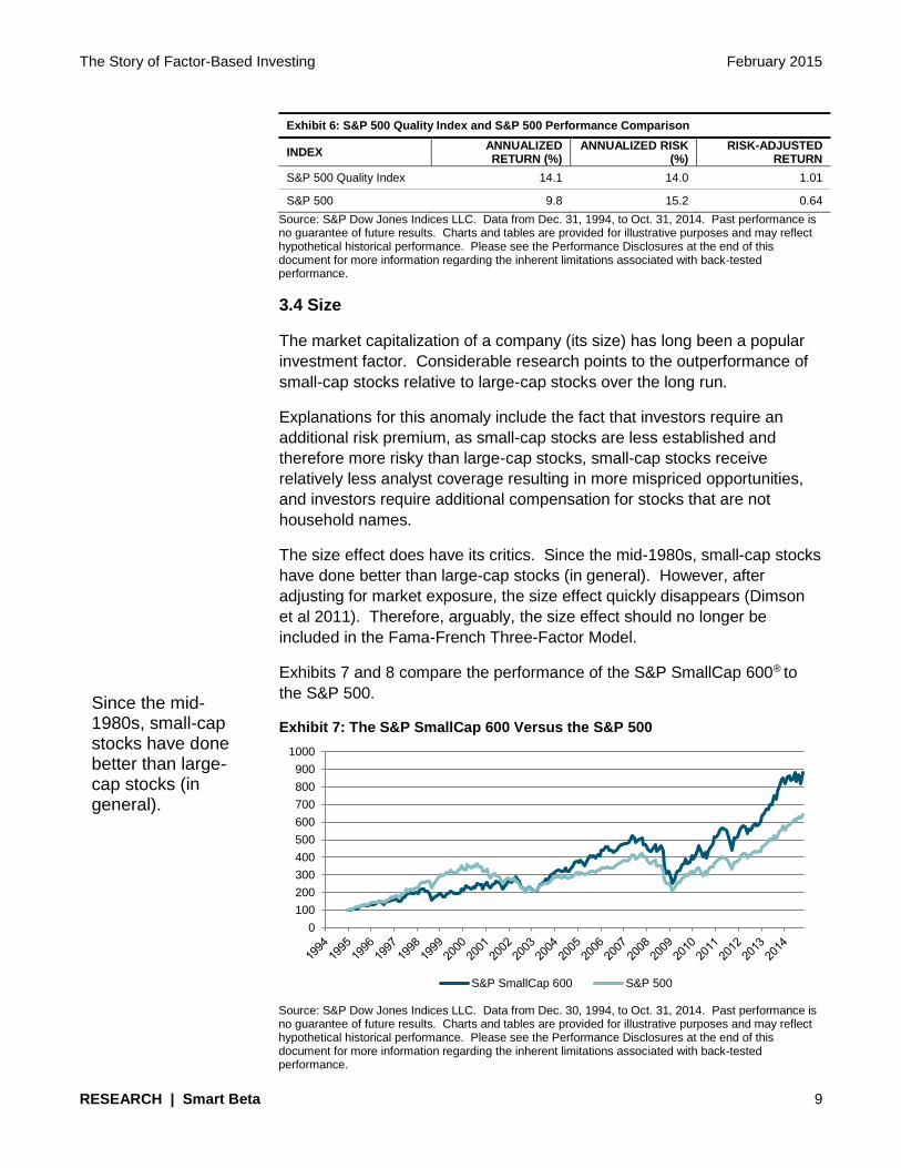
Exhibits 7 and 8 compare the performance of the S&P SmallCap 600® to

the S&P 500.

Exhibit 7: The S&P SmallCap 600 Versus the S&P 500


0

100

200

300

400

500

600

700

800

900

1000

S&P SmallCap 600 S&P 500

Since the mid-1980s, small-cap stocks have done better than large-cap stocks (in general).



Exhibit 8: S&P SmallCap 600 and S&P 500 Performance Comparison


ANNUALIZED RISK (%)


S&P SmallCap 600 11.6 18.9 0.61

S&P 500 9.8 15.2 0.64


The risk-adjusted return of the S&P SmallCap 600 is slightly lower than that

of the S&P 500, suggesting that the size effect has eroded since the mid-

1980s.

3.5 Corporate Finance: Share Repurchases

Share repurchases center on share buybacks, insider purchases, or a

combination of both. Share buybacks may provide information to investors

about future earnings and valuation of a company’s stock. Merton and

Rock (1985) argue that managers that anticipate higher future cash flows

are more likely to distribute cash in advance to their shareholders through

stock repurchases or cash dividends. Moreover, research by Ikenberry et

al (1995) suggests that management initiates buyback programs when it

believes its company’s stock is undervalued.

Share repurchase programs (unlike dividends) are not tied to a

preannounced policy. If a company needs to reduce its redistribution of

cash to shareholders, it can stop its repurchase program, while maintaining

its current dividend policy. This may help a company avoid the adverse

market reaction that is often associated with dividend cuts (Lintner 1956).

The agency problem may be at play too. Managers have the capacity to

put their own interests ahead of those of their shareholders. The main

concern for shareholders is that management may invest in projects with

poor returns in order to achieve growth. Easterbrook (1984) and Jensen

(1986) both argue that the potential for the misallocation of cash exists, and

that one way to mitigate such agency costs is for management to return

capital to shareholders via dividends or share repurchases.

Insider purchases can reflect promising news about a stock or the

confidence that senior managers have in their companies. Of note, the

reverse is equally true. This can be simply calculated as the number of

insiders purchasing shares minus the number of insiders selling.

The S&P 500 Buyback Index targets the share repurchase anomaly. This

equally weighted index is designed to measure the performance of the top

Share repurchase programs (unlike dividends) are not tied to a preannounced policy.



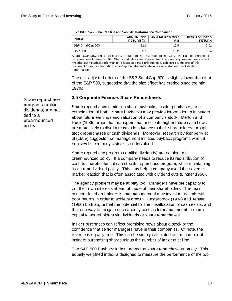
100 stocks with the highest buyback ratios11 in the S&P 500. Its

performance is compared to its parent index in Exhibits 9 and 10.

Exhibit 9: The S&P 500 Buyback Index Versus the S&P 500


Exhibit 10: Performance Comparison


ANNUALIZED RISK (%)


S&P 500 Buyback Index 14.8 15.9 0.93

S&P 500 9.2 15.0 0.62


3.6 Volatility

First documented in the early 1970s, the inverse relationship between

equity risk and return contradicts the conventional hypothesis that higher

risk should result in higher expected return (Friend and Blume 1970). In

addition, it called into question the CAPM and many of its multifactor

extensions. In terms of pricing, Equations 4 and 5 clearly state that the

expected return of an asset is a function of its covariance with risk factors.

Furthermore, the asset’s specific risk component (under expectation) was

dropped, as it was modeled as a normal random variable with a mean of

zero. Possibly, the CAPM fails because it does not address imperfect

market structure and participants’ preferences for holding some assets over

others for exogenous reasons.

Recent studies documenting this inverse relationship include Ang et al

(2009) and Dutt and Humphery-Jenner (2013). Explanations for the

11 The buyback ratio is defined as the monetary amount of cash paid for repurchasing common shares (under the program) in the last four

calendar quarters divided by the total market capitalization of common shares at the beginning of the buyback period.

0

200

400

600

800

1000

1200

1400

1600

1800

2000

S&P 500 Buyback Index S&P 500

The inverse relationship between equity risk and return contradicts the conventional hypothesis that higher risk should result in higher expected return.



phenomenon differ, and a clear consensus seems distant. Theories

include imperfect market structure, illiquidity, and lottery preferences.

Idiosyncratic volatility can be computed using the Fama-French Three-

Factor Model. Alternatively, the much simpler approach of using total

volatility over a given period achieves remarkably effective results, as

demonstrated by the S&P Europe 350 Low Volatility Index. This index

measures the performance of the 100 least volatile stocks in the S&P

Europe 350. Constituents are weighted relative to the inverse of their

corresponding volatility, with the least volatile stocks receiving the highest

weights.

Exhibit 11: The S&P Europe 350 Low Volatility Index Versus the S&P Europe 350

Source: S&P Dow Jones Indices LLC. Data from Oct. 30, 1998, to Oct. 31, 2014. Past performance is no guarantee of future results. Charts and tables are provided for illustrative purposes and may reflect hypothetical historical performance. Please see the Performance Disclosures at the end of this document for more information regarding the inherent limitations associated with back-tested performance.

Exhibit 12: S&P Europe 350 Low Volatility Index and S&P Europe 350 Performance Comparison


ANNUALIZED RISK (%)


S&P Europe 350 Low Volatility Index

9.1 11.1 0.82

S&P Europe 350 4.8 15.6 0.31

Source: S&P Dow Jones Indices LLC. Data from Oct. 30, 1998, to Oct. 31, 2014. Past performance is no guarantee of future results. Charts and tables are provided for illustrative purposes and may reflect hypothetical historical performance. Please see the Performance Disclosures at the end of this document for more information regarding the inherent limitations associated with back-tested performance.

Incorporating the volatility factor in a portfolio may provide some drawdown

protection. Over the period studied, the maximum drawdown was 42% for

the S&P Europe 350 Low Volatility Index, with a maximum drawdown

duration of 5.1 years. Over the same period, the parent index reported

53% and 6.3 years, respectively.

0

50

100

150

200

250

300

350

400

450

S&P Europe 350 Low Volatility Index S&P Europe 350Idiosyncratic volatility can be computed using the Fama-French Three-Factor Model.



4.0 COMMODITY FACTORS

4.1 Roll Yield

Roll yield strategies harvest a systematic risk premium by purchasing

contracts at the longer end of the futures curve. In theory, producers sell

long-dated contracts, often at a discount, to hedge their production output.

On the other hand, consumers purchase short-dated contracts at a

premium to secure near-term consumption. This dynamic leads to a

structural systematic risk premium. In reality, the shape of the curve is

determined by the overall impact generated from the interaction between all

market participants, including nonindustrial players such as passive

investors and hedge funds. All of these participants will have their own

objectives and time horizons (Kang and Ung 2013).

The simplest strategy to capture this risk premium is to roll into futures

contracts of a predefined maturity, such as the three-month contract. The

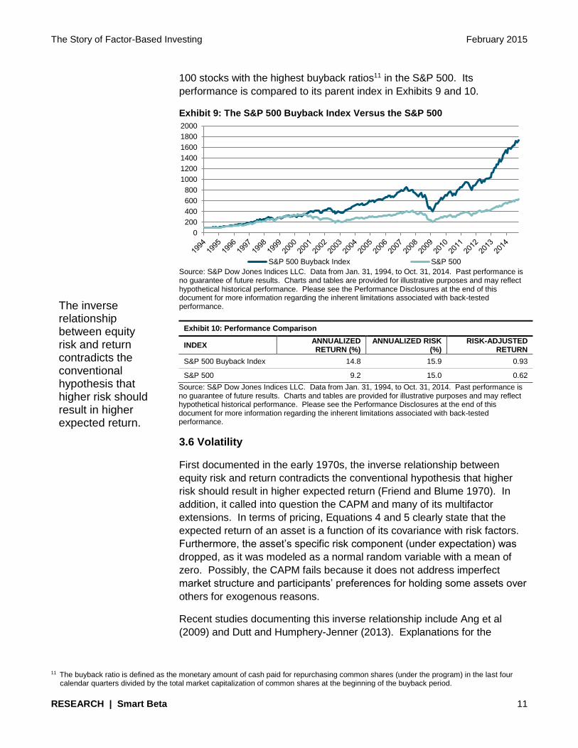
S&P GSCI 3-Month Forward Index employs this approach. More dynamic

strategies aim to minimize the effect from contango or maximize the effect

from backwardation12 by adopting a different roll strategy with respect to the

term structure of the commodity concerned—for instance, the S&P GSCI

Dynamic Roll.

Exhibit 13: The S&P GSCI Dynamic Roll Versus the S&P GSCI


12 Contango is a situation where the futures price of a commodity is above the expected spot price. Backwardation is the market condition

wherein the price of a futures contract is trading below the expected spot price at contract maturity. Therefore, the opposite market condition to backwardation is contango.

0

200

400

600

800

1000

1200

1400

1600

S&P GSCI Dynamic Roll S&P GSCI

Roll yield strategies harvest a systematic risk premium by purchasing contracts at the longer end of the futures curve.



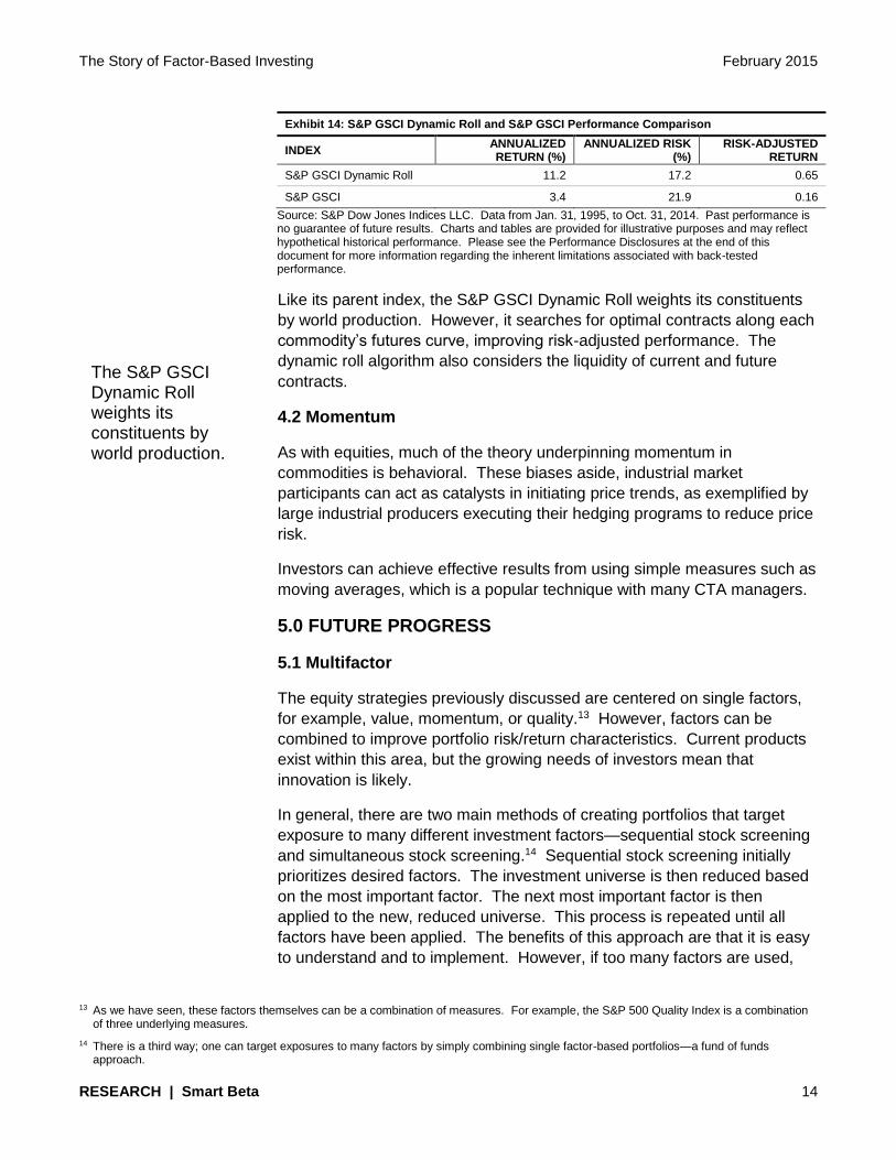
Exhibit 14: S&P GSCI Dynamic Roll and S&P GSCI Performance Comparison


ANNUALIZED RISK (%)


S&P GSCI Dynamic Roll 11.2 17.2 0.65

S&P GSCI 3.4 21.9 0.16


Like its parent index, the S&P GSCI Dynamic Roll weights its constituents

by world production. However, it searches for optimal contracts along each

commodity’s futures curve, improving risk-adjusted performance. The

dynamic roll algorithm also considers the liquidity of current and future

contracts.

4.2 Momentum

As with equities, much of the theory underpinning momentum in

commodities is behavioral. These biases aside, industrial market

participants can act as catalysts in initiating price trends, as exemplified by

large industrial producers executing their hedging programs to reduce price

risk.

Investors can achieve effective results from using simple measures such as

moving averages, which is a popular technique with many CTA managers.

5.0 FUTURE PROGRESS

5.1 Multifactor

The equity strategies previously discussed are centered on single factors,

for example, value, momentum, or quality.13 However, factors can be

combined to improve portfolio risk/return characteristics. Current products

exist within this area, but the growing needs of investors mean that

innovation is likely.

In general, there are two main methods of creating portfolios that target

exposure to many different investment factors—sequential stock screening

and simultaneous stock screening.14 Sequential stock screening initially

prioritizes desired factors. The investment universe is then reduced based

on the most important factor. The next most important factor is then

applied to the new, reduced universe. This process is repeated until all

factors have been applied. The benefits of this approach are that it is easy

to understand and to implement. However, if too many factors are used,

13 As we have seen, these factors themselves can be a combination of measures. For example, the S&P 500 Quality Index is a combination

of three underlying measures.

14 There is a third way; one can target exposures to many factors by simply combining single factor-based portfolios—a fund of funds approach.

The S&P GSCI Dynamic Roll weights its constituents by world production.



resulting portfolios may be too concentrated, with portfolio-specific risks

unacceptably high.

Simultaneous screening applies only one screen to a combination of all

chosen factors. Normally, factors are combined using the Z-score method.

For example, a simple value and momentum model might assign 50%

weight to the value Z-score and 50% weight to the momentum Z-score.

This approach allows greater flexibility within the portfolio design stage, as

practitioners can tinker with the weights to control portfolio outputs. By

contrast, portfolios created from sequential screening tend to strongly

reflect the first dominant screen. For more sophisticated simultaneous

screening models, algorithms can be designed to adjust the weights

applied to factors to better align with the current market or economic

environment. This informs dynamic weighting schemes.

The S&P Europe 350 Low Volatility High Dividend Index employs the

sequential stock screening approach. This equally weighted index (with 50

constituents) attempts to capture both the value and low volatility

anomalies.

Exhibit 15: S&P Europe 350 Low Volatility High Dividend Index Versus S&P Europe 350 Index


Exhibit 16: S&P Europe 350 Low Volatility High Dividend Index and S&P Europe 350 Performance Comparison

INDEX ANNUALIZED RETURN

(%) ANNUALIZED

RISK (%) RISK-ADJUSTED

RETURN

S&P Europe 350 Low Volatility High Dividend Index

9.5 15.6 0.61

S&P Europe 350 2.5 15.7 0.16


0

50

100

150

200

250

300

350

400

S&P Europe 350 Low Volatility High Dividend Index S&P Europe 350

The S&P Europe 350 Low Volatility High Dividend Index attempts to capture both the value and low volatility anomalies.



Exhibits 15 and 16 show that combining both factors in an index can work

well. Of note, the order of the screens is important. Within this index, the

dominant screen aims to harvest the value risk premium by selecting high

dividend yielding stocks. Unlike the S&P 500 Dividend Aristocrats, which

seeks consistency in dividend payments as well as yield, this index’s initial

screen is based purely on yield.15 However, a form of quality control is

implemented through the use of the second screen (volatility). This second

screen mitigates against possible value traps by eliminating stocks with

high price volatility.

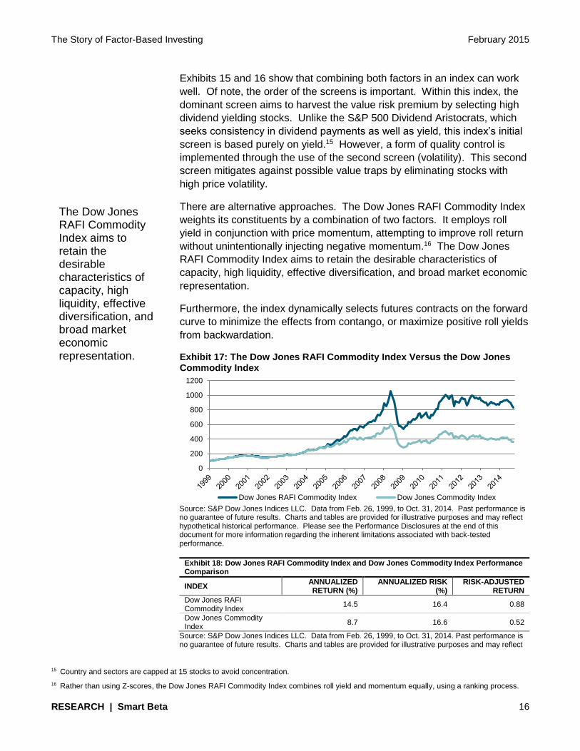
There are alternative approaches. The Dow Jones RAFI Commodity Index

weights its constituents by a combination of two factors. It employs roll

yield in conjunction with price momentum, attempting to improve roll return

without unintentionally injecting negative momentum.16 The Dow Jones

RAFI Commodity Index aims to retain the desirable characteristics of

capacity, high liquidity, effective diversification, and broad market economic

representation.

Furthermore, the index dynamically selects futures contracts on the forward

curve to minimize the effects from contango, or maximize positive roll yields

from backwardation.

Exhibit 17: The Dow Jones RAFI Commodity Index Versus the Dow Jones Commodity Index

Source: S&P Dow Jones Indices LLC. Data from Feb. 26, 1999, to Oct. 31, 2014. Past performance is no guarantee of future results. Charts and tables are provided for illustrative purposes and may reflect hypothetical historical performance. Please see the Performance Disclosures at the end of this document for more information regarding the inherent limitations associated with back-tested performance.

Exhibit 18: Dow Jones RAFI Commodity Index and Dow Jones Commodity Index Performance Comparison


ANNUALIZED RISK (%)


Dow Jones RAFI Commodity Index

14.5 16.4 0.88

Dow Jones Commodity Index

8.7 16.6 0.52

Source: S&P Dow Jones Indices LLC. Data from Feb. 26, 1999, to Oct. 31, 2014. Past performance is no guarantee of future results. Charts and tables are provided for illustrative purposes and may reflect

15 Country and sectors are capped at 15 stocks to avoid concentration.

16 Rather than using Z-scores, the Dow Jones RAFI Commodity Index combines roll yield and momentum equally, using a ranking process.

0

200

400

600

800

1000

1200

Dow Jones RAFI Commodity Index Dow Jones Commodity Index

The Dow Jones RAFI Commodity Index aims to retain the desirable characteristics of capacity, high liquidity, effective diversification, and broad market economic representation.



hypothetical historical performance. Please see the Performance Disclosures at the end of this document for more information regarding the inherent limitations associated with back-tested performance.

The index risk/return profile improves on its parent index, providing a

stronger inflation hedge, and it is arguably a more suitable commodity

component of diversified global portfolios.

5.2 Risk Premia

The indices discussed so far combine the market and the targeted risk

premia. Therefore, market risk accounts for a considerable portion of the

total risk in each of these strategies. However, it is possible to isolate risk

premia. For example, a value index seeks to provide exposure to both the

market and the value risk premium. Taking a long position in this index and

a corresponding short position in a growth index would remove a large

proportion of market risk, while isolating the value risk premium. Similarly,

the small-cap risk premium can be isolated by taking a long position in a

small-cap index and a short position in a large-cap index. Combining both

examples effectively isolates the risk premia (excluding market)

incorporated in the Fama-French Three-Factor Model.

The same approach can be implemented within both the commodities and

fixed income spaces. For example, a long position based on the 10+-Year

U.S. Treasury bond index and a short position based on an index at the

short end of the yield curve, say 1-3-Year U.S. Treasury bonds, would

isolate the term spread. A similar approach could be taken to isolate the

credit and high-yield spreads, as well.

During the financial crisis of 2008-2009, many investors who believed that

their portfolios were diversified discovered that they were not. Holdings

across multiple asset classes, including hedge funds and private equity,

and different strategies, failed to mitigate the market meltdown because

their portfolios were still exposed to broad common factors. The risk

premia approach could allow investors to harvest return-producing units

across asset classes, while possibly removing a large proportion of market

risk. Moreover, evidence exists that over the long term, many of these

units are barely correlated with each other, thus providing clear

diversification benefits.

Innovation in this area is likely, as investors seek to build more robust

portfolios.

5.3 Fixed Income

A large amount of research and development has expanded the range of

factor-based indices and equity products. By comparison, relatively little

work has been done in the fixed income sphere.

During the financial crisis of 2008-2009, many investors who believed that their portfolios were diversified discovered that they were not.



Traditional fixed income indices are market-value weighted—the size of the

issue multiplied by its price. Therefore, investors find themselves exposed

to countries or corporations that are more indebted. In addition, as these

indices are price based, if a bond increases in price, it receives higher

weighting within the index. As a result, the index automatically increases

the weights of more expensive bonds. Conversely, these indices

systematically reduce the exposure of more inexpensive bonds that offer a

higher yield.

Products that address the suboptimal weighting of traditional, market-value

fixed income indices are likely to become an important investment tool.

Moreover, fixed income return drivers (factors), such as the term structure,

credit spread, and high yield, are likely to become prominent in fixed

income products in the future. Finally, more sophisticated products may

acquire information from the financial statements, such as cash flows, total

assets, and interest cover, to build more robust fixed income indices.

6.0 CONCLUSIONS

The economic intuition behind the CAPM is important—factors underlying

assets determine asset risk premiums, and these risk premiums provide

compensation for investors bearing systematic risks. On the other hand,

specific risks can be diversified away and are not rewarded with excess

returns.

Since the CAPM’s formulation in the 1960s, academics and practitioners

have continually improved it. Pricing anomalies such as value, momentum,

and quality have provided excess returns within the equity domain. The

same principles are increasingly applied to commodities, and awareness is

growing within the fixed income sphere as well.

The economic intuition behind factors is important. Back-tested

performance alone is insufficient to execute an investment program.

Moreover, we now know that strategies must be tested over multiple

periods to understand performance over different business cycles and

economic regimes, to help construct more robust portfolios. When

combining factors, cross correlations can reveal diversification benefits.

Factor combinations should always have an economic rationale.

Weighting schemes are important. For example, index constituents can be

equally weighted, which is relatively agnostic. Alternatively, they can be

transform weighted (market capitalization multiplied by a factor score),

retaining some of the parent index’s characteristics. Finally, weights can be

determined purely by factor score (beta), providing a strong solution for

those that find traditional market capitalization indices unacceptably

inefficient.

It is likely that the potential advantages of factor-based products, particularly their transparent and systematic rules and relatively low costs, will mean practitioners continue to utilize and develop them.



It is likely that the potential advantages of factor-based products,

particularly their transparent and systematic rules and relatively low costs,

will mean practitioners continue to utilize and develop them. The next few

years will be interesting.



BIBLIOGRAPHY

Ang, A., Hodrick, J., Xing, Y., Zhang, X., (2009). High idiosyncratic volatility and low returns:

International and further U.S. evidence. Journal of Financial Economics. Vol 91, 1-23.

Carhart, M.M., (2012). On Persistence in Mutual Fund Performance. Journal of Finance. 52 (1), 57-82.

Daniel, K., D., Hirshleifer, D., Subrahmanyam, A., (2001). Overconfidence, arbitrage, and equilibrium

asset pricing. Journal of Finance. Vol 56 (3), 921-965.

Dimson, E., Marsh, P., Staunton, M., (2011). Credit Suisse Global Investment Returns Sourcebook.

Credit Suisse Research Institute.

Dutt, T. and Humphery-Jenner, M., (2013). Stock Return Volatility, operating performance and stock

returns: International evidence on drivers of the ‘low volatility’ anomaly. Journal of Banking and

Finance. Vol 37 (3) 99 – 1017.

Easterbrook, F.H., (1984). Two agency-cost explanations of dividends. American Economic Review. 74

(4), 650-660.

Fama, E.F. and French, K.R., (1993). Common risk factors in the returns on stocks and bonds. Journal

of Financial Economics. 33 (1), 3-56.

Fama, E.F. and French, K.R., (1996). Multifactor Explanations of Asset Pricing Anomalies. Journal of

Finance. 51, 55-84.

Friend, I. and Blume, M., (1970). Measurement of Portfolio Performance under uncertainty. American

Economic review. Vol 65, 561 – 575.

Hong, H., Lim, T., Stein, J. C., (2000). Bad news travels slowly: Size, analyst coverage, and the

profitability of momentum strategies. Journal of Finance. Vol 55 (1) 265-295.

Ikenberry, D., Lakonishok, J., Vermaelen, T., (1995). Market underreaction to open market share

repurchases. Journal of Financial Economics. 39 (2), 181-208.

Jegadeesh, N. and Titman, S., (1993). Returns to buying winners and selling losers: Implications for

stock market efficiency. Journal of Finance. Vol 48 (1), 65-91.

Jensen, M.C., (1986). Agency costs of free cash flow, corporate finance and takeovers. American

Economic Review. 26, May, 323-329.

Kang, X. and Ung, D., (2013). Alternative Beta Strategies in Commodities. S&P Dow Jones Indices

Research Paper.

Lakonishok, J., Shleifer, A., Vishny, R. W., (1994). Contrarian Investment, Extrapolation, and Risk.

Journal of Finance. Vol 69 (5), 1541-1578.

Lintner, J., (1956). Distributions of income of corporations among dividends, retained earnings and taxes.

American Economic Review. 46, May, 97-113.

http://linker.westminster.ac.uk/sfx_wmin?ctx_ver=Z39.88-2004&ctx_enc=info:ofi/enc:UTF-8&ctx_tim=2012-04-10T08%3A21%3A47IST&url_ver=Z39.88-2004&url_ctx_fmt=infofi/fmt:kev:mtx:ctx&rfr_id=info:sid/primo.exlibrisgroup.com:primo3-Article-sciversesciencedirect_elsevier&rft_val_fmt=info:ofi/fmt:kev:mtx:&rft.genre=article&rft.atitle=Market%20underreaction%20to%20open%20market%20share%20repurchases&rft.jtitle=Journal%20of%20Financial%20Economics&rft.btitle=&rft.aulast=Ikenberry&rft.auinit=&rft.auinit1=&rft.auinitm=&rft.ausuffix=&rft.au=Ikenberry,%20David&rft.aucorp=&rft.date=1995&rft.volume=39&rft.issue=2&rft.part=&rft.quarter=&rft.ssn=&rft.spage=181&rft.epage=208&rft.pages=181-208&rft.artnum=&rft.issn=0304-405X&rft.eissn=&rft.isbn=&rft.sici=&rft.coden=&rft_id=info:doi/10.1016/0304-405X(95)00826-Z&rft.object_id=&svc_val_fmt=info:ofi/fmt:kev:mtx:sch_svc&svc.fulltext=yes&rft_dat=%3csciversesciencedirect_elsevier%3e0304-405X(95)00826-Z%3c/sciversesciencedirect_elsevier%3e&rft.eisbn=&rft_id=info:oai/

http://linker.westminster.ac.uk/sfx_wmin?ctx_ver=Z39.88-2004&ctx_enc=info:ofi/enc:UTF-8&ctx_tim=2012-04-10T08%3A21%3A47IST&url_ver=Z39.88-2004&url_ctx_fmt=infofi/fmt:kev:mtx:ctx&rfr_id=info:sid/primo.exlibrisgroup.com:primo3-Article-sciversesciencedirect_elsevier&rft_val_fmt=info:ofi/fmt:kev:mtx:&rft.genre=article&rft.atitle=Market%20underreaction%20to%20open%20market%20share%20repurchases&rft.jtitle=Journal%20of%20Financial%20Economics&rft.btitle=&rft.aulast=Ikenberry&rft.auinit=&rft.auinit1=&rft.auinitm=&rft.ausuffix=&rft.au=Ikenberry,%20David&rft.aucorp=&rft.date=1995&rft.volume=39&rft.issue=2&rft.part=&rft.quarter=&rft.ssn=&rft.spage=181&rft.epage=208&rft.pages=181-208&rft.artnum=&rft.issn=0304-405X&rft.eissn=&rft.isbn=&rft.sici=&rft.coden=&rft_id=info:doi/10.1016/0304-405X(95)00826-Z&rft.object_id=&svc_val_fmt=info:ofi/fmt:kev:mtx:sch_svc&svc.fulltext=yes&rft_dat=%3csciversesciencedirect_elsevier%3e0304-405X(95)00826-Z%3c/sciversesciencedirect_elsevier%3e&rft.eisbn=&rft_id=info:oai/



Merton, M. and Rock, K., (1985). Dividend policy Under Asymmetric Information. Journal of Finance. 40

(4), 1031-1051.

Ross, S.A., (1976). The Arbitrage Theory of Capital Asset Pricing. Journal of Economic Theory. 13, 341-

360.

Qian, E.E., Hua, R.H., Sorenson, E.H., (2007). Quantitative Equity Portfolio Management. Chapman &

Hall/CRC.



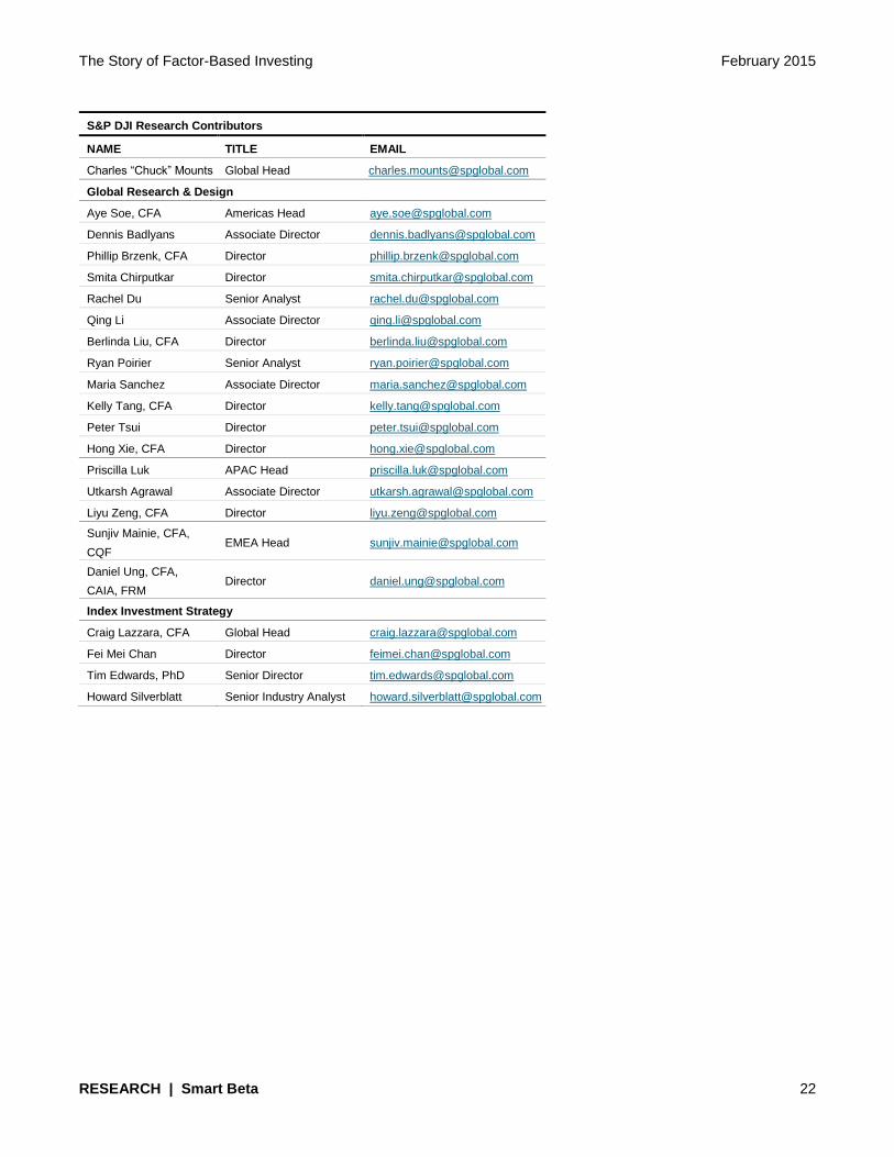
S&P DJI Research Contributors

NAME TITLE EMAIL

Charles “Chuck” Mounts Global Head [email protected]

Global Research & Design

Aye Soe, CFA Americas Head [email protected]

Dennis Badlyans Associate Director [email protected]

Phillip Brzenk, CFA Director [email protected]

Smita Chirputkar Director [email protected]

Rachel Du Senior Analyst [email protected]

Qing Li Associate Director [email protected]

Berlinda Liu, CFA Director [email protected]

Ryan Poirier Senior Analyst [email protected]

Maria Sanchez Associate Director [email protected]

Kelly Tang, CFA Director [email protected]

Peter Tsui Director [email protected]

Hong Xie, CFA Director [email protected]

Priscilla Luk APAC Head [email protected]

Utkarsh Agrawal Associate Director [email protected]

Liyu Zeng, CFA Director [email protected]

Sunjiv Mainie, CFA,

CQF EMEA Head [email protected]

Daniel Ung, CFA,

CAIA, FRM Director [email protected]

Index Investment Strategy

Craig Lazzara, CFA Global Head [email protected]

Fei Mei Chan Director [email protected]

Tim Edwards, PhD Senior Director [email protected]

Howard Silverblatt Senior Industry Analyst [email protected]








PERFORMANCE DISCLOSURE

The S&P GSCI was launched on May 1, 1991, the S&P 500 Dividend Aristocrats Index was launched on May 2, 2005, the S&P Europe 350 Momentum Index was launched on Nov. 18, 2014, the S&P 500 Quality Index was launched on July 8, 2014, the S&P 500 SmallCap 600 Index was launched on Oct. 28, 1994, the S&P 500 Buyback Index was launched on Nov. 29, 2012, the S&P Europe 350 Low Volatility Index was launched on July 9, 2012, the S&P Europe 350 Equal Weight Index was launched on Jan. 21, 2014, the S&P GSCI Dynamic Roll Index was launched on Jan. 26, 2011, the S&P Europe 350 Low Volatility High Dividend Index was launched on Jan. 22, 2014, the Dow Jones RAFI Commodity Index was launched on Sept. 10, 2014, the S&P Europe 350 Index was launched on Oct. 7, 1998, the S&P 500 Index was launched on March 4, 1957, and the Dow Jones Commodity Index was launched on Oct. 26, 2011. All information for an index prior to its launch date is back-tested. Back-tested performance is not actual performance, but is hypothetical. The back-test calculations are based on the same methodology that was in effect on the launch date. Complete index methodology details are available at www.spdji.com. It is not possible to invest directly in an index.

S&P Dow Jones Indices defines various dates to assist our clients in providing transparency on their products. The First Value Date is the first day for which there is a calculated value (either live or back-tested) for a given index. The Base Date is the date at which the Index is set at a fixed value for calculation purposes. The Launch Date designates the date upon which the values of an index are first considered live: index values provided for any date or time period prior to the index’s Launch Date are considered back-tested. S&P Dow Jones Indices defines the Launch Date as the date by which the values of an index are known to have been released to the public, for example via the company’s public website or its datafeed to external parties. For Dow Jones-branded indicates introduced prior to May 31, 2013, the Launch Date (which prior to May 31, 2013, was termed “Date of introduction”) is set at a date upon which no further changes were permitted to be made to the index methodology, but that may have been prior to the Index’s public release date.

Past performance of the Index is not an indication of future results. Prospective application of the methodology used to construct the Index may not result in performance commensurate with the back-test returns shown. The back-test period does not necessarily correspond to the entire available history of the Index. Please refer to the methodology paper for the Index, available at www.spdji.com for more details about the index, including the manner in which it is rebalanced, the timing of such rebalancing, criteria for additions and deletions, as well as all index calculations.

Another limitation of using back-tested information is that the back-tested calculation is prepared with the benefit of hindsight. Back-tested information reflects the application of the index methodology and selection of index constituents in hindsight. No hypothetical record can completely account for the impact of financial risk in actual trading. For example, there are numerous factors related to the equities, fixed income, or commodities markets in general which cannot be, and have not been accounted for in the preparation of the index information set forth, all of which can affect actual performance.

The Index returns shown do not represent the results of actual trading of investable assets/securities. S&P Dow Jones Indices LLC maintains the Index and calculates the Index levels and performance shown or discussed, but does not manage actual assets. Index returns do not reflect payment of any sales charges or fees an investor may pay to purchase the securities underlying the Index or investment funds that are intended to track the performance of the Index. The imposition of these fees and charges would cause actual and back-tested performance of the securities/fund to be lower than the Index performance shown. As a simple example, if an index returned 10% on a US $100,000 investment for a 12-month period (or US $10,000) and an actual asset-based fee of 1.5% was imposed at the end of the period on the investment plus accrued interest (or US $1,650), the net return would be 8.35% (or US $8,350) for the year. Over a three year period, an annual 1.5% fee taken at year end with an assumed 10% return per year would result in a cumulative gross return of 33.10%, a total fee of US $5,375, and a cumulative net return of 27.2% (or US $27,200).

http://www.spdji.com/

http://www.spdji.com/



GENERAL DISCLAIMER

Copyright © 2016 by S&P Dow Jones Indices LLC, a part of S&P Global. All rights reserved. Standard & Poor’s ®, S&P 500 ® and S&P ® are registered trademarks of Standard & Poor’s Financial Services LLC (“S&P”), a subsidiary of S&P Global. Dow Jones ® is a registered trademark of Dow Jones Trademark Holdings LLC (“Dow Jones”). Trademarks have been licensed to S&P Dow Jones Indices LLC. Redistribution, reproduction and/or photocopying in whole or in part are prohibited without written permission. This document does not constitute an offer of services in jurisdictions where S&P Dow Jones Indices LLC, Dow Jones, S&P or their respective affiliates (collectively “S&P Dow Jones Indices”) do not have the necessary licenses. All information provided by S&P Dow Jones Indices is impersonal and not tailored to the needs of any person, entity or group of persons. S&P Dow Jones Indices receives compensation in connection with licensing its indices to third parties. Past performance of an index is not a guarantee of future results.

It is not possible to invest directly in an index. Exposure to an asset class represented by an index is available through investable instruments based on that index. S&P Dow Jones Indices does not sponsor, endorse, sell, promote or manage any investment fund or other investment vehicle that is offered by third parties and that seeks to provide an investment return based on the performance of any index. S&P Dow Jones Indices makes no assurance that investment products based on the index will accurately track index performance or provide positive investment returns. S&P Dow Jones Indices LLC is not an investment advisor, and S&P Dow Jones Indices makes no representation regarding the advisability of investing in any such investment fund or other investment vehicle. A decision to invest in any such investment fund or other investment vehicle should not be made in reliance on any of the statements set forth in this document. Prospective investors are advised to make an investment in any such fund or other vehicle only after carefully considering the risks associated with investing in such funds, as detailed in an offering memorandum or similar document that is prepared by or on behalf of the issuer of the investment fund or other vehicle. Inclusion of a security within an index is not a recommendation by S&P Dow Jones Indices to buy, sell, or hold such security, nor is it considered to be investment advice.

These materials have been prepared solely for informational purposes based upon information generally available to the public and from sources believed to be reliable. No content contained in these materials (including index data, ratings, credit-related analyses and data, research, valuations, model, software or other application or output therefrom) or any part thereof (Content) may be modified, reverse-engineered, reproduced or distributed in any form or by any means, or stored in a database or retrieval system, without the prior written permission of S&P Dow Jones Indices. The Content shall not be used for any unlawful or unauthorized purposes. S&P Dow Jones Indices and its third-party data providers and licensors (collectively “S&P Dow Jones Indices Parties”) do not guarantee the accuracy, completeness, timeliness or availability of the Content. S&P Dow Jones Indices Parties are not responsible for any errors or omissions, regardless of the cause, for the results obtained from the use of the Content. THE CONTENT IS PROVIDED ON AN “AS IS” BASIS. S&P DOW JONES INDICES PARTIES DISCLAIM ANY AND ALL EXPRESS OR IMPLIED WARRANTIES, INCLUDING, BUT NOT LIMITED TO, ANY WARRANTIES OF MERCHANTABILITY OR FITNESS FOR A PARTICULAR PURPOSE OR USE, FREEDOM FROM BUGS, SOFTWARE ERRORS OR DEFECTS, THAT THE CONTENT’S FUNCTIONING WILL BE UNINTERRUPTED OR THAT THE CONTENT WILL OPERATE WITH ANY SOFTWARE OR HARDWARE CONFIGURATION. In no event shall S&P Dow Jones Indices Parties be liable to any party for any direct, indirect, incidental, exemplary, compensatory, punitive, special or consequential damages, costs, expenses, legal fees, or losses (including, without limitation, lost income or lost profits and opportunity costs) in connection with any use of the Content even if advised of the possibility of such damages.

S&P Dow Jones Indices keeps certain activities of its business units separate from each other in order to preserve the independence and objectivity of their respective activities. As a result, certain business units of S&P Dow Jones Indices may have information that is not available to other business units. S&P Dow Jones Indices has established policies and procedures to maintain the confidentiality of certain non-public information received in connection with each analytical process.

In addition, S&P Dow Jones Indices provides a wide range of services to, or relating to, many organizations, including issuers of securities, investment advisers, broker-dealers, investment banks, other financial institutions and financial intermediaries, and accordingly may receive fees or other economic benefits from those organizations, including organizations whose securities or services they may recommend, rate, include in model portfolios, evaluate or otherwise address.

contributor the story of factor-based investing€¦ · · 2017-02-01the story of factor-based...

Documents