control of natural gas catalytic partial oxidation for ...annastef/fuelcellpdf/fpscontcstsub.pdf ·...

IEEE TRANSACTION ON CONTROL SYSTEM TECHNOLOGY, VOL. XX, NO. Y, MONTH 2003 1

Control of Natural Gas Catalytic Partial

Oxidation for Hydrogen Generation in Fuel

Cell Applications

Jay T. Pukrushpan, Anna G. Stefanopoulou, Subbarao Varigonda

Lars M. Pedersen, Shubhro Ghosh, Huei Peng

Abstract

A fuel processor that reforms natural gas to hydrogen-rich mixture to feed the anode field of fuel cell

stack is considered. The first reactor that generates the majority of the hydrogen in the fuel processor is

based on catalytic partial oxidation of the methane in the natural gas. We present a model-based control

analysis and design for a fuel processing system that manages natural gas flow and humidified atmospheric

air flow in order to regulate (i) the amount of hydrogen in the fuel cell anode and (ii) the temperature of

the catalytic partial oxidation reactor during transient power demands from the fuel cell.

Linear feedback analysis and design is used to identify the limitation of a decentralized controller

and the benefit of a multivariable controller. Further analysis unveils the critical controller cross-coupling

term that contributes to the superior performance of the multivariable controller.

Keywords

Fuel Cell, Fuel Processor, Hydrogen Generation, Multivariable Feedback, Linear Control, Dynamics.

Support is provided by NSF CMS-021332. Matching funds to these grants were provided by United Technologies

J.T. Pukrushpan, A.G. Stefanopoulou and H. Peng are with the Department of Mechanical Engineering at the

University of Michigan, Ann Arbor, Michigan.

S. Varigonda, L.M. Pedersen and S. Ghosh are with the United Technologies Research Center, East Hartford,

Connecticut.

March 26, 2003 DRAFT

Pukrushpan et al. FPS Control 2

I. Introduction

Fuel Cells are considered for stationary (residential and commercial) and mobile (au-

tomotive and portable) power generation due to their high efficiency and environmental

friendliness. Inadequate infrastructure for hydrogen refueling, distribution, and storage

makes the fuel processor technology an important part of the fuel cell system for both sta-

tionary and mobile applications. For residential applications, fueling the fuel cell system

using natural gas is often preferred because of its wide availability and extended distribu-

tion system [1]. Common methods of converting natural gas to hydrogen include steam

reforming and partial oxidation. The most common method, steam reforming, which is

endothermic, is well suited for steady-state operation and can deliver a relatively high con-

centration of hydrogen [2], but it suffers from a poor transient operation [3]. On the other

hand, the partial oxidation offers several other advantages such as compactness, rapid-

startup, and responsiveness to load changes [1], but delivers lower conversion efficiency.

WGS1

Water

Air fromAtmosphere

Natural Gas

Air

H2 rich gasto FC stack

WGS2 PROXHDS

BLOHEX

MIX CPOX

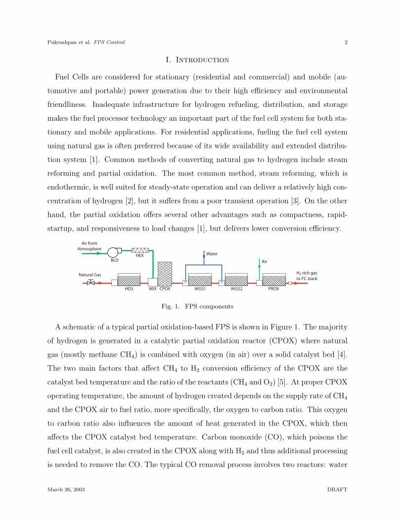
Fig. 1. FPS components

A schematic of a typical partial oxidation-based FPS is shown in Figure 1. The majority

of hydrogen is generated in a catalytic partial oxidation reactor (CPOX) where natural

gas (mostly methane CH4) is combined with oxygen (in air) over a solid catalyst bed [4].

The two main factors that affect CH4 to H2 conversion efficiency of the CPOX are the

catalyst bed temperature and the ratio of the reactants (CH4 and O2) [5]. At proper CPOX

operating temperature, the amount of hydrogen created depends on the supply rate of CH4

and the CPOX air to fuel ratio, more specifically, the oxygen to carbon ratio. This oxygen

to carbon ratio also influences the amount of heat generated in the CPOX, which then

affects the CPOX catalyst bed temperature. Carbon monoxide (CO), which poisons the

fuel cell catalyst, is also created in the CPOX along with H2 and thus additional processing

is needed to remove the CO. The typical CO removal process involves two reactors: water



gas shift (WGS) and preferential oxidation (PROX) [6], which are represented, in this

study, as if they perfectly remove the CO with the introduction of water and air. More

details on the FPS chemical reactions are given in Section II.

During changes in the stack current, the fuel processor needs to (i) quickly regulate the

amount of hydrogen in the fuel cell stack (anode) to avoid starvation or wasted hydrogen

[7] and (ii) maintain a desired temperature of the CPOX catalyst bed for high conversion

efficiency [8]. Accurate control and coordination of the fuel processor reactant flows can

prevent both large deviation of hydrogen concentration in the anode and large excursion

of CPOX catalyst bed temperature. A control-oriented nonlinear model of the natural gas

fuel processing system is developed in Section III with a focus on the dynamic behaviors

associated with the flows and pressure in the FPS and also the temperature of the CPOX.

The two main performance variables are the anode hydrogen mole fraction [9] and the

CPOX catalyst bed temperature [5]. The two control actuators are the fuel (CH4) valve

command and the CPOX air blower command. The control problem is formulated in

Section IV and a linearized model derived in Section V is used in the control analysis and

design.

Typical fuel processing systems rely on a decentralized (single-input single-output) con-

trol of the air blower command to control CPOX temperature and of the fuel valve com-

mand to control the anode hydrogen concentration. In Section VI, an analysis using the

relative gain array method confirms the appropriateness of the traditional input-output

pairs for the decentralized control. The study also shows large interactions between the

two loops at high frequencies and different operating conditions. These interactions can be

more efficiently handled with multivariable control which is studied in Section VIII. The

linear quadratic optimal control method is used to design the controller (LQR) and the

state estimator (LQG) that achieves a significant improvement in the CPOX temperature

regulation as compared to the decentralized controller. It is shown in Section IX that

the regulation of the anode H2 mole fraction depends strongly on the speed of the fuel

valve command while the improvement in the CPOX temperature regulation is due to the

coordination of both inputs.



II. Fuel Processing System (FPS)

Figure 1 illustrates the components in a natural gas fuel processing system (FPS) [10].

Natural gas (mostly methane CH4) is supplied to the FPS from either a high-pressure

tank or a high-pressure pipeline. The main air flow is supplied to the system by a blower

(BLO) which draws air from the atmosphere. The air is then heated in the heat exchanger

(HEX). The hydro-desulfurizer (HDS) is used to remove sulfur present in the natural gas

stream [1], [11]. The de-sulfurized natural gas stream is then mixed with the heated air

flow in the mixer (MIX). The mixture is then passed through the catalyst bed inside the

catalytic partial oxidizer (CPOX) where CH4 reacts with oxygen to produce H2. There

are two main chemical reactions taking place in the CPOX: partial oxidation (POX) and

total oxidation (TOX) [5], [12]:

(POX) CH4 +1

2O2 → CO + 2H2 (1)

(TOX) CH4 + 2O2 → CO2 + 2H2O (2)

Heat is released from both reactions. However, TOX reaction releases more heat than

POX reaction. The difference in the rates of the two reactions depends on the selectivity,

S, defined as

S =rate of CH4 reacting in POX

total rate of CH4 reacting(3)

The selectivity depends strongly on the oxygen to carbon ratio (O2 to CH4), denoted by

λO2C

, entering the CPOX [5]. Hydrogen is created only in POX reaction and, therefore,

it is preferable to promote this reaction in the CPOX. However, the heat generated from

POX reaction is not sufficient to maintain CPOX temperature. Thus, promoting TOX

reaction is also required. Carbon monoxide (CO) is also created along with H2 in the POX

reaction as can be seen in (1). Since CO poisons the fuel cell catalyst, it is eliminated

using both the water gas shift converter (WGS) and the preferential oxidizer (PROX).

As illustrated in Figure 1, there are typically two WGS reactors operating at different

temperatures [3], [6]. In the WGS, water is injected into the gas flow in order to promote

a water gas shift reaction:

(WGS) CO + H2O → CO2 + H2 (4)



Note that even though the objective of WGS is to eliminate CO, hydrogen is also created

from the WGS reaction. The level of CO in the gas stream after WGS is normally still

high for fuel cell operation and thus oxygen is injected (in the form of air) into the PROX

reactor to react with the remaining CO:

(PROX) 2CO + O2 → 2CO2 (5)

The amount of air injected into the PROX is typically twice the amount that is needed to

maintain the stoichiometric reaction in (5) [3], [13].

III. Control-Oriented FPS Model

The FPS model is developed with a focus on the dynamic behaviors associated with the

flows and pressures in the FPS and also the temperature of the CPOX.

Several assumptions are made in order to simplify the FPS model. Since the control of

WGS and PROX reactants are not studied, the two components are lumped together as

one volume and the combined volume is called WROX (WGS+PROX). It is also assumed

that both components are perfectly controlled to obtain desired conversion and operating

temperatures. Furthermore, because the amount of H2 created in WGS is proportional

to the amount of CO that reacts in WGS (Reaction (4)), which in turn, is proportional

to the amount of H2 generated in CPOX (Reaction (1)), it is assumed that the amount

of H2 generated in the WGS is always a fixed percentage of the amount of H2 produced

in the CPOX. The de-sulfurization process in the HDS is not modeled and thus the HDS

is viewed as a storage volume. It is assumed that the pressures and compositions of the

air entering the blower and of the natural gas entering the HDS are constant. Natural

gas is considered as pure methane CH4. Additionally, any temperature other than the

CPOX temperature is assumed constant and the effect of temperature changes on the

pressure dynamics is assumed negligible. The volume of CPOX is relatively small and its

dynamics are captured in the mixer. It is also assumed that all reactions are fast and

reach equilibrium before the flow exit the reactors. Finally, all gases obey the ideal gas

law and all gas mixtures are perfect mixtures. Figure 2 illustrates the simplified system

and state variables used in the model.

The dynamic states in the model, shown also in Figure 2, are blower speed, ωblo, heat



HDS

HEX

hds

hex

mixmix wroxwrox

BLO

PCH4Pair PH2

anPH2

P

P

bloωcpox P

T anP

TANK

ANODEMIX CPOX WROX(WGS+PROX)

Fig. 2. FPS dynamic model

exchanger pressure, phex, HDS pressure, phds, mixer CH4 partial pressure, pmixCH4

, mixer air

partial pressure, pmixair , CPOX temperature, Tcpox, WROX (combined WGS and PROX)

volume pressure, pwrox, WROX hydrogen partial pressure, pwroxH2

, anode pressure, pan,

and anode hydrogen partial pressure, panH2

. We provide here a brief outline of the model.

Although, we use the linearized model for the control analysis and design, the physical

interpretation of the states helps in the control design and in interpreting the results.

The speed of the blower, ωblo, is modeled as a first-order dynamic system with time

constant τb. The governing equation is

dωblo

dt=

1

τb

(ublo

100ω0 − ωblo) (6)

where ublo is the blower command signal (range between 0 and 100) and ω0 is the maxi-

mum blower speed (3600rpm). The gas flow rate through the blower is modeled, Wblo =

f(ωblo,phex

patm), using a blower map. Mass conservation with the ideal gas law through the

isothermal assumption is used to model the pressure dynamics of the gas in all component

volumes considered in the system. In any volume that does not involve any reaction,

mixture composition is unchanged and the total pressure of the gas is used as the state

(phex in HEX and phds in HDS). On the other hand, gas compositions in MIX, WROX and

fuel cell anode (AN) changes due to reactions involved. The changes in gas composition

in these volumes are described with additional partial pressures of the important species.

In general, the pressure dynamics of a gas n in a volume m is governed by

dpmn

dt=

RTm

MnVm

(Wmn,in − Wm

n,out) (7)

where R is the universal gas constant, Vm is the component gas volume, Mn is the molar

mass of species n, and Tm is the temperature of the gas in the volume. The mass flow rate



Wmn,in is the rate (in (kg/s)) of the species n going into the volume m which includes the

species flow into the volume and the species produced (from the reaction) in the volume.

The flow rate Wmn,out are the rate of species n going out of the volume including the species

flow rate exiting the volume and the rate of species reacted in the reaction.

The total flow rate, W , between two volumes is, in general, calculated from pressure

differential, p1 − p2, using the orifice equation with a turbulent flow assumption

W = W0

√p1 − p2

∆p0

(8)

where W0 and ∆p0 are the nominal air flow rate and the nominal pressure drop of the

orifice, respectively. The flow rate of a constituent species n between the volumes is a

function of the total gas flow and the mole fraction of the species n in the upstream

volume. The flow rate of fuel (natural gas) into HDS, Whds,in, is, in addition, a function

of the valve input, uvalve,

Whds,in =(uvalve

100

)W0,valve

√ptank − phds

∆p0,valve

(9)

where ptank is the fuel tank or supply line pressure.

The conversion of the gases in CPOX is based on the reactions in (1) and (2) and the

selectivity defined in (3), which is a function of the oxygen to carbon ratio in MIX, λO2C

:

λO2C

= yatmO2

pmixair

pmixCH4

(10)

where yatmO2

is the oxygen mole fraction of the atmospheric air. The energy conservation

principle is used to model the changes in CPOX temperature.

mcpxCcpxP

dTcpox

dt=

inlet en-

thalpy

flow

−

outlet

en-

thalpy

flow

+

heat

from re-

actions

(11)

where mcpx (kg) and CcpxP (J/kg·K) are mass and specific heat capacity of the catalyst

bed, respectively. The terms on the right hand side of (11) are determined based on

the reactants and products gas of the CPOX reactions. Further details of the model are

presented in [14].



IV. Control Problem Formulation

As previously discussed, the main objectives of the FPS controller are (i) to protect the

stack from damage due to H2 starvation (ii) to protect CPOX from overheating and (iii) to

keep overall system efficiency high, which includes high stack H2 utilization and high FPS

CH4-to-H2 conversion. Objectives (ii) and (iii) are related since maintaining the desired

CPOX temperature during steady-state implies proper regulation of the oxygen-to-carbon

ratio which corresponds to high FPS conversion efficiency.

Two performance variables that need to be regulated are the anode hydrogen mole

fraction, yH2

,

yH2

=pan

H2

pan(12)

calculated based on (7) and the CPOX temperature, Tcpox, calculated based on (11). They

are chosen based on the following rationale. High Tcpox can cause the catalyst bed to be

overheated and be permanently damaged. Low Tcpox results in a low CH4 reaction rate in

the CPOX [5] and potential methane slip. Large deviations of yH2

are undesirable. On

one hand, a low value of yH2

means anode H2 starvation [9], [15] which can permanently

damage the fuel cell structure. On the other hand, a high value of yH2

means small

hydrogen utilization which results in a waste of hydrogen.

In this control study, we assume that all CH4 that enters the CPOX reacts without any

methane slip. Note that these assumptions reduce the validity of the model for large Tcpox

deviations. The effect of the modeling error due to these assumptions can degrade the

performance of the model-based controller. However, achieving one of the control goals,

which is the regulation of Tcpox, will ensure that this modeling error remains small.

The H2 valve actuator dynamics are ignored. The stack current, Ist, is considered as an

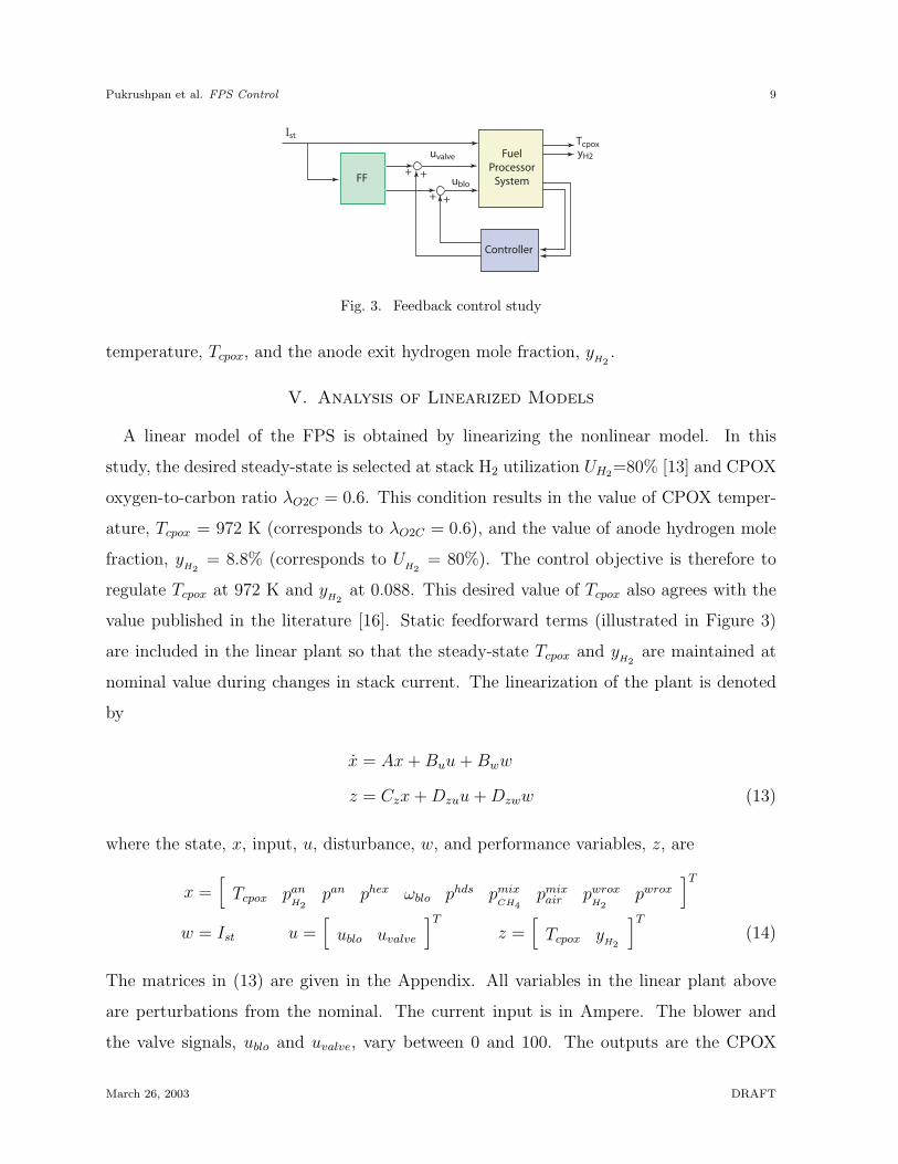
exogenous input that is measured. Since the exogenous input is measured, we consider a

two degrees of freedom (2DOF) controller based on feedforward and feedback, as shown

in Figure 3. The two control inputs, u, are the air blower signal, ublo, and the fuel

valve signal, uvalve. The feedforward terms that provide the valve and the blower signals

that reject the steady-state effect of current to the outputs are integrated in the plant:

u∗(Ist) =[

u∗blo(Ist) u∗

valve(Ist)]T

. The value of u∗ is obtained by nonlinear simulation

and can be implemented with a lookup table. The performance variable are the CPOX



FF

uvalve

TcpoxyH2

ublo

Ist

FuelProcessor

System+ +

++

Controller

Fig. 3. Feedback control study

temperature, Tcpox, and the anode exit hydrogen mole fraction, yH2

.

V. Analysis of Linearized Models

A linear model of the FPS is obtained by linearizing the nonlinear model. In this

study, the desired steady-state is selected at stack H2 utilization UH2=80% [13] and CPOX

oxygen-to-carbon ratio λO2C = 0.6. This condition results in the value of CPOX temper-

ature, Tcpox = 972 K (corresponds to λO2C = 0.6), and the value of anode hydrogen mole

fraction, yH2

= 8.8% (corresponds to UH2

= 80%). The control objective is therefore to

regulate Tcpox at 972 K and yH2

at 0.088. This desired value of Tcpox also agrees with the

value published in the literature [16]. Static feedforward terms (illustrated in Figure 3)

are included in the linear plant so that the steady-state Tcpox and yH2

are maintained at

nominal value during changes in stack current. The linearization of the plant is denoted

by

x = Ax + Buu + Bww

z = Czx + Dzuu + Dzww (13)

where the state, x, input, u, disturbance, w, and performance variables, z, are

x =[

Tcpox panH2

pan phex ωblo phds pmixCH4

pmixair pwrox

H2pwrox

]T

w = Ist u =[

ublo uvalve

]T

z =[

Tcpox yH2

]T

(14)

The matrices in (13) are given in the Appendix. All variables in the linear plant above

are perturbations from the nominal. The current input is in Ampere. The blower and

the valve signals, ublo and uvalve, vary between 0 and 100. The outputs are the CPOX



temperature in Kelvin and the anode hydrogen mole fraction in percent. In the transfer

function form, we can represent the plant as

z =[

Gw G] w

u

(15)

The nonlinear plant model is linearized at three different current (load) levels that

correspond to the 30%, 50%, and 80% of the plant power level. The Bode plots and step

responses of the linear plants that are obtained from different system power levels are

shown in Figures 4 and 5. For clarity, the units of current is (×10 Amp). Note first that

the static feedforward controller does well in rejecting the effect from Ist to yH2

and Tcpox in

steady-state. The H2 recovery using feedforward is, however, relatively slow. A feedback

controller is, thus, needed to speed up the system behavior and to reduce the sensitivity

introduced by modeling uncertainties.

From: uvalveFrom: ublo

200

-100

0

100

200

0.01 10 100 0.01

10 100 0.01

10 100 -360

0

360To:

yH

2

100

-50

0

50

100From: Ist (10A)

-720

-360

0

360

To:

Tcp

ox

Frequency (rad/sec)

Magnitude (dB)

Magnitude (dB) Magnitude (dB) Magnitude (dB)

Magnitude (dB)Magnitude (dB)

Phase (deg) Phase (deg) Phase (deg)

Phase (deg)Phase (deg)Phase (deg)

30%50%80%

Gw1

Gw1

Gw2

Gw2

G11

G11

G21

G22

G12

G21

G12

G22

Fig. 4. Bode plot of linearized models at 30%, 50%, and 80% power

The responses of the output due to step changes in the actuator signals, in Figure 5,

show a strongly coupled system. The fuel dynamics are slower than the air dynamics,

primarily due to the large HDS volume. Note that a right half plane (RHP) zero exists in



-60

-40

-20

0

20

40

60From: Ist

To:

Tcp

ox

0 20 40 60-2

-1

0

1

2

3

4

To:

yH

2

From: ublo

0 20 40 60

From: uvalve

0 20 40 60

30%50%80%

Step Response

Time (sec)

Am

plitu

de

Fig. 5. Step responses of linearized models at 30%, 50%, and 80% power

the path ublo → yH2

can be easily detected from the initial inverse response of the yH2

due

to a step change in ublo. Moreover, as can be seen in the step responses from ublo to yH2

,

the RHP zero that causes the non-minimum phase behavior moves closer to the imaginary

axis and causes larger initial inverse response at low power level (30%). The linearization

of the system at the 50% power level is used in the control study in the following sections.

VI. Input-Output Pairing

One of the most common approaches to controlling a multi-input multi-output (MIMO)

system is to use a diagonal controller, which is often referred to as a decentralized con-

troller. The decentralized control works well if the plant is close to diagonal which means

that the plant can be considered as a collection of individual single-input single-output

(SISO) sub-plants with no interaction among them. In this case, the controller for each

sub-plant can be designed independently. If the interaction between the loops is large,

then the performance of the decentralized controller may be poor.

Due to the non-minimum phase zero in the ublo → yH2

transfer function, the preferred

pairing choices are ublo → Tcpox pair and uvalve → yH2

pair. This pairing choice is also

confirmed by the relative gain array (RGA) matrix [17] of G ,

RGA = G × (G−1)T (16)



at zero frequency is

RGA(0 rad/s) =

2.302 −1.302

−1.302 2.302

(17)

The RGA can also be used to assess the loop interactions. Large off-diagonal elements

of the RGA matrix indicates large loop interactions. A plot of the magnitude difference

between the diagonal and off-diagonal elements of the RGA matrices in Figure 6 shows

that the interactions increase at high frequencies [18], [17]. At low power levels, the values

of the off-diagonal elements of the RGA matrix are even higher than the diagonal elements

(|RGA11| − |RGA12| < 0), indicating large coupling. At these frequencies, we can expect

poor performance from a decentralized controller.

0.01 0.1 1 10 100 -0.4

-0.2

0

0.2

0.4

0.6

0.8

1

Difference between diagonal and off diagonal elements

|RG

A11

| - |R

GA

21|

Frequency (rad/s)

30%50% 80%

Fig. 6. Difference between diagonal and off-diagonal elements of the RGA matrix at different frequencies

for three power setpoints

VII. Decentralized Control

To illustrate the effect of the interactions, we design several PI controllers for the two

single-input single-output (SISO) systems that correspond to the diagonal subsystem of

G, i.e., ublo → Tcpox (G(1, 1)), and uvalve → yH2

(G(2, 2)). The diagram in Figure 7 shows

the decentralized controller.

The gains of the PI controllers, K11 and K22, are chosen after iterations to achieve

the best performance subject to actuator activity. Since fast response of yH2 is more

critical, the PI controller in the fuel loop (uvalve → yH2

) is tuned first to achieve fast



K11

K22G

Gw

uvalve

Tcpox

yH2

ublo

Ist

Fig. 7. Decentralized Control

response of yH2

without saturating the valve. Then, to achieve fast regulation of Tcpox,

we also tune the second PI for fast air loop while avoiding blower saturation. Figure 8

shows the response using fast controllers in both loops in dashed line, for the system at

medium power (50%). Due to the large interaction as RGA predicted, the performance

of the decentralized controller with fast controller in both loops degrades significantly

when the system operate at low power as shown in Figure 9. One way to compensate

for the interaction is to create a bandwidth separation between the two loops. Since

designing the air loop to be faster than the fuel loop is not feasible with a PI controller

due to blower magnitude constraints, the air loop is detuned to be slower than the fuel

loop. Figures 8 and 9 also show the performance of the decentralized controller that has

bandwidth separation. It can be seen that the speed of Tcpox regulation has to be sacrificed

to prevent the degradation effect of the system interactions on the decentralized controller.

The PI controllers chosen are given in Table II.

-100

-80

-60

-40

-20

0

To

Tcp

ox (

dB)

-80

-70

-60

-50

-40

-30

-20

-10

To

yH2

(dB

)

Frequency (rad/s)

0 2 4 6 8 10 12 14 16 18 20-0.4

-0.2

0

0.2

0.4

0.6

0.8

1

Tcp

ox

0 2 4 6 8 10 12 14 16 18 20-0.15

-0.1

-0.05

0

0.05

yH2

Time (sec)

Open LoopFastAir, FastFuelSlowAir, FastFuel

0.01 0.1 1 10 100

0.01 0.1 1 10 100

Fig. 8. Bode magnitude and unit step response of model at 50% power

Note that more complex decentralized controllers can be used (high-order or PID, for



-100

-80

-60

-40

-20

0

20

To

Tcp

ox (

dB)

-80

-60

-40

-20

0

To

yH2

(dB

)

Frequency (rad/s)

0 2 4 6 8 10 12 14 16 18 20

-0.4

-0.2

0

0.2

0.4

0.6

Tcp

ox

0 2 4 6 8 10 12 14 16 18 20

-0.1

-0.05

0

0.05

0.1

0.15

yH2

Time (sec)

Open LoopFastAir, FastFuelSlowAir, FastFuel

0.01 0.1 1 10 100

0.01 0.1 1 10 100

Fig. 9. Bode magnitude and unit step response of model at 30% power

example). The PI controller tuning here is used only to illustrate the effect of plant

interactions and difficulties in tuning the PI controllers without systematic MIMO control

tools. The conclusion from this section is that the large plant interactions illustrated by

Figure 6 must be considered in the control design.

An interesting point is that, for the decentralized PI controller, the bandwidth of the

air loop needs to be smaller than the bandwidth of the fuel loop. This was the only way

to achieve a bandwidth separation within the blower saturation constraints. However, if a

higher order controller is allowed, a higher closed loop bandwidth can be achieved. Indeed,

as we show later in Section IX, a high-order decentralized controller using the diagonal

terms of a full MIMO controller achieves a decade higher bandwidth than the fuel loop

without saturating the blower.

VIII. Multivariable Control

We show in the previous section that the interactions in the plant limit the performance

of the decentralized controller. In this section, we assess the improvement gained by

a controller developed using a multivariable and model-based control design techniques.

The controller is designed using linear quadratic (LQ) methodology.

To eliminate steady-state error, we add to the controller the integrators on the two

performance variables, Tcpox and yH2

. Note that, we assume that these two variables can



be directly and instantaneously measured. The state equations of the integrators are

d

dt

q1

q2

=

T ref

cpox − Tcpox

yrefH2

− yH2

(18)

where T refcpox = 972 K and yref

H2= 8.8 % are the desired values of Tcpox and y

H2, respectively.

In the linear domain, the desired deviation from the reference values is thus zero for all

current commands. The controller is designed with the objective of minimizing the cost

function

J =

∫ ∞

0

zT Qzz + qT QIq + uT Ru dt (19)

where Qz, QI , and R are weighting matrices on the performance variables, z, integrator

state, q, and control input, u, respectively.

The control law that minimizes (19) is in the form

u = −KP (x − xd) − KIq = −K

(x − xd)

q

(20)

where K is the control gain and x is the estimate of plant state. The values of KP and

KI are given in Table III in the Appendix. Variable xd in (20) is a function of Ist and

can be viewed as the desired values of the states that give the desired value of z = 0. In

other words, the term Kpxd is an additional feedforward term that compensates for the

changes in the output steady-state value due to the feedback. As a result, this additional

feedforward term is a function of the feedback gain, Kp. The value of xd can be found by

simulation or by the linear plant matrices (13). As it is based on the linear model, the value

of xd calculated will be different from the actual desired state in the nonlinear plant. The

error in xd definitely influences the steady-state error of the performance variables, Tcpox

and yH2

. The integral control implemented through the augmented integrators (18) then

becomes more critical. The fact that xd is not accurate must be taken into account when

choosing the weighting between Qz and QI . Large integrator gain slows down the response,

thus relatively small QI shows a better (faster) performance in linear design. However, the

response in nonlinear simulation with small QI gives poor steady-state performance since

the performance is based heavily on the proportional part of the controller and therefore

suffers from the error in xd. Thus, if a more accurate value of xd can not be obtained,



the transient performance must be compromised in order to get satisfactory steady-state

performance of the controller through the integral part. Alternatively, a more accurate xd

can be obtained by numerically solving the nonlinear simulation and stored in a lookup

table.

The estimate of the plant state, x, can be determined using the dynamic model of the

plant together with the available performance measurements. The observer state equations

are

˙x = Ax + Buu + Bww + L(z − z)

z = Czx + Dzuu + Dzww (21)

where x is the estimator state vector and L is the estimator gain (Table III) determined

based on LQG methodology.

The nonlinear simulation of the system with the decentralized PI feedback and with

the output observer-based feedback is shown in Figure 10. The output feedback gives

satisfactory performance in both yH2

and Tcpox regulations.

595 600 605 610 615960

980

1000

1020

1040

595 600 605 610 6150.02

0.04

0.06

0.08

0.1

0.12

Time (sec)

595 600 605 610 615150

200

250

Open LoopDecentralizedMIMO

595 600 605 610 61540

45

50

55

60

595 600 605 610 61540

60

80

100

Time (sec)

Tcpox

ublo

Ist

uvalve

yH2

Fig. 10. Comparison of decentralized PI controller and observer feedback in nonlinear simulation

IX. Insight Gained by the Multivariable Design

The combination of the state feedback control (20) and the state observer (21) results

in a model-based multivariable output-feedback controller. In transfer function form, the

controller can be written as

u = Cww + Cz =

Cw1

Cw2

w +

C11 C12

C21 C22

z (22)



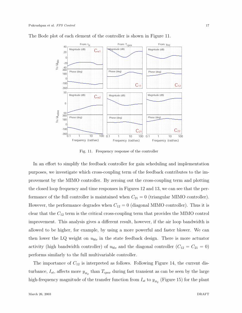
The Bode plot of each element of the controller is shown in Figure 11.

From: yH2From: Tcpox

50

0

50

To:

uva

lve

0.1 1 10 100 0.1 1 10 100 0.1 1 10 100 -360

-180

0

180

360

40

-20

0

20

40From: Ist

-360

-180

0

180

360To:

ubl

o

Frequency (rad/sec) Frequency (rad/sec)Frequency (rad/sec)

Magnitude (dB)

Phase (deg)

Magnitude (dB)

Phase (deg)

Magnitude (dB)

Phase (deg)

Magnitude (dB)

Phase (deg)

Magnitude (dB)

Phase (deg)

Magnitude (dB)

Phase (deg)

C11

Cw1

Cw2

C12

C21 C22

Fig. 11. Frequency response of the controller

In an effort to simplify the feedback controller for gain scheduling and implementation

purposes, we investigate which cross-coupling term of the feedback contributes to the im-

provement by the MIMO controller. By zeroing out the cross-coupling term and plotting

the closed loop frequency and time responses in Figures 12 and 13, we can see that the per-

formance of the full controller is maintained when C21 = 0 (triangular MIMO controller).

However, the performance degrades when C12 = 0 (diagonal MIMO controller). Thus it is

clear that the C12 term is the critical cross-coupling term that provides the MIMO control

improvement. This analysis gives a different result, however, if the air loop bandwidth is

allowed to be higher, for example, by using a more powerful and faster blower. We can

then lower the LQ weight on ublo in the state feedback design. There is more actuator

activity (high bandwidth controller) of ublo and the diagonal controller (C12 = C21 = 0)

performs similarly to the full multivariable controller.

The importance of C12 is interpreted as follows. Following Figure 14, the current dis-

turbance, Ist, affects more yH2

than Tcpox during fast transient as can be seen by the large

high-frequency magnitude of the transfer function from Ist to yH2

(Figure 15) for the plant



-100

-80

-60

-40

-20

0

-50

-45

-40

-35

-30

-25

-20

-15

-10

10-1

100

101

102

To:

yH

2

From: Ist

To:

Tcp

ox

Frequency (rad/sec)

Mag

nitu

de (

dB)

Full ControllerC21 = 0C12 = C21 = 0

Fig. 12. Closed-loop frequency response for analysis of elements in the feedback controllers

0 5 10 15 -0.08

-0.06

-0.04

-0.02

0

0.02

0.04

0 5 10 15-0.1

-0.08 -0.06 -0.04 -0.020

0.020.04

0 5 10 15 -0.15

-0.1

-0.05

0

0.05

0 5 10 150

0.1

0.2

0.3

0.4

0.5

Time (sec) Time (sec)

Tcpox ublo

uvalveyH2

Full ControllerC21 = 0C12 = C21 = 0

Fig. 13. Closed-loop time response for analysis of elements in the feedback controllers

G11

C12

C21

C22

C11

G12

G22

G21

ubloeTcpox

eyH2

TcpoxTcpox

yH2yH2 uvalve

ref

ref

++ +

-

+++ +

++

+

+

+ -

Gw1

Gw2

Ist

Fig. 14. Block Diagram of FPS plant and simplified controller



with feedforward control: Gw = Gw + GCw. The valve signal, uvalve, tries to reject the

10-1

100

101

102

-90

-80

-70

-60

-50

-40

-30

-20

-10

Mag

nitu

de (

dB)

Ist to TcpoxIst to yH2

Frequency (rad/sec)

Gw2

Gw1

Fig. 15. Frequency magnitude plot of the plant with dynamic feedforward part of the controller Gzw in

(IX)

effect of Gw2Ist to yH2

(see Figure 14) by using the feedback C22 term through G22. The

blower signal, on the other hand, cannot reject the Gw2Ist to yH2

through G21C12 because

of the non-minimum phase zero of G21 (zNMP

= 3.07).

Gw2Ist

1 + G21C12 + G22C22

� Gw2Ist

1 + G22C22

Indeed, Figure 11 shows that the magnitude of C12 is low at frequencies close to that of

the NMP zero. Meanwhile, the valve that tries hard to reject the Gw2Ist to yH2

causes

disturbances to Tcpox through the plant G12 interaction. The controller cross-coupling term

C12 is thus needed to compensate for the effect of uvalve to Tcpox by partially cancelling

G12C22 by G11C12 at certain frequencies.

Tcpox =G12C22 + G11C12

1 + G11C11

eyH2

≈ 0 ⇒ C12 ≈ −G−111 G12C22

Note that this partial cancellation involves the plant elements G11 and G12 that do not

change significantly for different power levels, as compared to G21 (see Figure 4). Thus the

benefit of the controller cross-coupling term C12 is maintained in full range of operating

power. If the air loop has high bandwidth, the G11C11 term can reject the disturbance by

itself and, then, controller C12 is not needed to cancel the interaction from the valve to

Tcpox.



Figure 11 also verifies that C21 does not contribute to the overall MIMO controller.

The magnitude of C21 is, in fact, relatively smaller than other feedback terms. At high

frequencies where the effect of Gw2Ist to yH2

is large, the term C21 is not used to help

regulating yH2

because the deviation in yH2

is not reflected in Tcpox measurement (Gw1Ist

is small). At low frequencies where Ist affects Tcpox, C21 may be used to help reduce Tcpox

error but will cause disturbance to the well-behaved fuel loop, thus C21 is also insignificant

at low frequencies.

By comparing the response of decentralized PI controller in Figure 10 and that of the

diagonal MIMO controller in Figure 13, we can see that the diagonal controller derived

from the MIMO controller outperforms the decentralized PI controller. This is achieved

as shown in Figure 16 because of the higher closed loop bandwidth of the air loop when

compared with the one of the PI-based controller. As seen in Figure 11, the high-order C11

term can have high bandwidth without having high gain and thus avoids blower saturation.

This can not be achieved using a PI controller. Indeed, Figure 11 verifies that the gain

of C11 is low at the frequencies where loop-interaction is large (see Figure 6 for the loop

interactions).

10-2

10 -1

100

101

102

From: yH2

10 -2

10 -1

100

101

102 -140

-120

-100

-80

-60

-40

-20

0

20

To:

yH

2

-150

-100

-50

0

50From: Tcpox

To:

Tcp

ox

Decentralized PIDiagonal MIMOFull MIMO

Frequency (rad/sec)

Fig. 16. Frequency (magnitude in dB) response from reference signal of closed loop system with MIMO

controller

In summary, the MIMO controller achieves a superior performance in comparison with

the decentralized PI controller due to two factors. First, the MIMO controller achieves a



high bandwidth on the air loop without saturating the actuator by achieving high band-

width without high gain. This is only feasible with high-order controllers. In hindsight

of the success of the C11 term of the MIMO controller, one can design a PID or a PI +

lead-lag controller that reproduces similar gain and phase to be used in the decentralized

controller.

Second, the MIMO controller achieves better coordination between the two actuators

by utilizing a cross-coupling term. The cross-coupling term acts in a “feedforward” sense

and changes the blower command based on how the fuel valve behaves. This partially

cancels the interaction between the fuel valve to the air loop. This partial cancellation,

luckily, involves plant elements that do not change significantly for different power levels.

Thus, without having explicitly designed for robustness, the MIMO controller maintains

its performance at all power levels.

X. Concluding Remarks

The control problem of hydrogen generation using catalytic partial oxidation and pre-

vention of fuel cell stack starvation is studied. The two-input two-output control problem

has the air blower and the fuel valve as inputs and the CPOX temperature and the anode

hydrogen mole fraction (anode starvation) as performance variables.

We show that tuning two PI controllers for the air and the fuel loops is difficult. More-

over, the closed loop performance is adversely affected by the intrinsic interaction between

the two loops. One way to prevent the performance degradation is to have bandwidth sepa-

ration between the two control loops. This introduces a compromise of the air-temperature

closed loop response in favor to the fuel-hydrogen loop.

On the other hand, a model-based high-order controller designed using linear multivari-

able methodologies, LQR-LQG in our case, can achieve very good response for a wide

range of operating conditions. Our analysis shows that the multivariable controller can be

simplified to a lower triangular controller where the blower command depends on both er-

rors in Tcpox and yH2 (or, equivalently, fuel valve). If the multivariable controller is further

simplified to a diagonal controller (no cross-coupling between control inputs and errors in

the performance variables), the closed loop performance degrades with respect to the full

multivariable controller but it still outperforms the two PI-based closed loop performance.



Apart from these application specific recommendations, our analysis demonstrated that

the improvement of the MIMO controller exists for fundamental and physically motivated

reasons. This understanding made the non-control engineers involved in this project ap-

preciate the complexity in the model-based control design and support the next phase of

experimental validation.

XI. Acknowledgements

The authors would like to thank Thordur Runolfsson, Jonas Eborn, Christoph Haug-

stetter and Scott Bortoff at the United Technology Research Center for their help and

valuable comments.

References

[1] A.L. Dicks, “Hydrogen generation from natural gas for the fuel cell systems of tomorrow,” Journal of Power

Sources, vol. 61, pp. 113–124, 1996.

[2] S. Ahmed and M. Krumpelt, “Hydrogen from hydrocarbon fuels for fuel cells,” International Journal of

Hydrogen Energy, vol. 26, pp. 291–301, 2001.

[3] L.F. Brown, “A comparative study of fuels for on-board hydrogen production for fuel-cell-powered automo-

biles,” International Journal of Hydrogen Energy, vol. 26, pp. 381–397, 2001.

[4] V. Recupero, L. Pino, R.D. Leonardo, M. Lagana, and G. Maggio, “Hydrogen generator, via catalytic partial

oxidation of methane for fuel cells,” Journal of Power Sources, vol. 71, pp. 208–214, 1998.

[5] J. Zhu, D. Zhang, and K.D. King, “Reforming of CH4 by partial oxidation: thermodynamic and kinetic

analyses,” Fuel, vol. 80, pp. 899–905, 2001.

[6] K. Ledjeff-Hey, J. Roses, and R. Wolters, “CO2-scrubbing and methanation as purification system for PEFC,”

Journal of Power Sources, vol. 86, pp. 556–561, 2000.

[7] D.Z. Megede, “Fuel processors for fuel cell vehicles,” Journal of Power Sources, vol. 106, pp. 35–41, 2002.

[8] L. Pino, V. Recupero, S. Beninati, A.K. Shukla, M.S. Hegde, and P.Bera, “Catalytic partial-oxidation of

methane on a ceria-supported platinum catalyst for application in fuel cell electric vehicles,” Applied Catalysis

A: General, vol. 225, pp. 63–75, 2002.

[9] T.E. Springer, R. Rockward, T.A. Zawodzinski, and S. Gottesfeld, “Model for polymer electrolyte fuel cell

operation on reformate feed,” Journal of The Electrochemical Society, vol. 148, pp. A11–A23, 2001.

[10] C.E. Thomas, B.D. James, F.D. Lomax Jr, and I.F. Kuhn Jr, “Fuel options for the fuel cell vehicle: hydrogen,

methanol or gasoline?,” International Journal of Hydrogen Energy, vol. 25, pp. 551–567, 2000.

[11] T.H. Gardner, D.A. Berry, K.D. Lyons, S.K. Beer, and A.D. Freed, “Fuel processor integrated H2S catalytic

partial oxidation technology for sulfur removal in fuel cell power plants,” Fuel, vol. 81, pp. 2157–2166, 2002.

[12] A.L. Larentis, N.S. de Resende, V.M.M. Salim, and J.C. Pinto, “Modeling and optimization of the combined

carbon dioxide reforming and partial oxidation of natural gas,” Applied Catalysis, vol. 215, pp. 211–224, 2001.

[13] E.D. Doss, R. Kumar, R.K. Ahluwalia, and M. Krumpelt, “Fuel processors for automotive fuel cell systems:

a parametric analysis,” Journal of Power Sources, vol. 102, pp. 1–15, 2001.



[14] Jay Tawee Pukrushpan, Modeling and Control of Fuel Cell Systems and Fuel Processors, Ph.D. thesis,

University of Michigan, 2003.

[15] R-H Song, C-S Kim, and D.R. Shin, “Effects of flow rate and starvation of reactant gases on the performance

of phosphoric acid fuel cells,” Journal of Power Sources, vol. 86, pp. 289–293, 2000.

[16] C.R.H. de Smet, M.H.J.M. de Croon, R.J. Berger, G.B. Marin, and J.C. Schouten, “Design of adiabatic fixed-

bed reactors for the partial oxidation of methane to synthesis gas. Application to production of methanol and

hydrogen-for-fuel-cells,” Chemical Engineering Science, vol. 56, pp. 4849–4861, 2001.

[17] Sigurd Skogestad and Ian Postlethwaite, Multivariable Feedback Control: Analysis and Design, Wiley, 1996.

[18] Manfred Morari and Evanghelos Zafiriou, Robust Process Control, Prentice Hall, 1997.

Appendix

TABLE I FPS linear model system matrices

-0.074 0 0 0 0 0 -3.53 1.0748 0 1E-06 0 0 0

0 -1.468 -25.3 0 0 0 0 0 2.5582 13.911 0 0 -0.328

0 0 -156 0 0 0 0 0 0 33.586 0 0 -0.024

0 0 0 -124.5 212.63 0 112.69 112.69 0 0 0 0 0

0 0 0 0 -3.333 0 0 0 0 0 0.12 0 0.0265

0 0 0 0 0 -32.43 32.304 32.304 0 0 0 0.1834 0.0504

0 0 0 0 0 331.8 -344 -341 0 9.9042 0 0 0

0 0 0 221.97 0 0 -253.2 -254.9 0 32.526 0 0 0

0 0 2.0354 0 0 0 1.8309 1.214 -0.358 -3.304 0 0 0

0.0188 0 8.1642 0 0 0 5.6043 5.3994 0 -13.61 0 0 0

1 0 0 0 0 0 0 0 0 0 0 0 0

0 0.994 -0.088 0 0 0 0 0 0 0 0 0 0

A

Cz

Bu

Dzu

Bw

Dzw

TABLE II Decentralized PI controllers

Controller Transfer Function

K11 0.0135 (5.6s+1)s

K22 0.165 (21s+1)s



TABLE III FPS controller gains

1.4054 0.18237 0.02904 1.0661 39.04 -6.6114 -0.70528 0.60367 0.76664 0.93881

-0.13028 1.1503 -0.13157 -0.24436 -8.422 6.1105 0.61755 -0.13879 3.787 0.12691

-1.2071 -0.16911

0.18907 -0.89972

469.67 138.59

5.6245 818.34

-93.622 -12.759

-742.29 -99.077

-30.245 -4.7928

-795.89 -104.2

-2149.2 -392.69

1400.7 294.09

1559.8 3547.1

-430.89 -58.728

KP

KI

L


control of natural gas catalytic partial oxidation for ...annastef/fuelcellpdf/fpscontcstsub.pdf ·...

Documents