control of vehicle platoons for highway safety and efficient utility
TRANSCRIPT

J Syst Sci Complex (20XX) XX: 1–28
Control of Vehicle Platoons for Highway Safety and
Efficient Utility: Consensus with Communications and
Vehicle Dynamics∗
Le Yi WANG · Ali SYED · George YIN · Abhilash PANDYA · Hongwei ZHANG
DOI:
Received: x x 20xx / Revised: x x 20xx
c©The Editorial Office of JSSC & Springer-Verlag Berlin Heidelberg 2013
Abstract Platoon formation of highway vehicles is a critical foundation for autonomous or semi-
autonomous vehicle control for enhanced safety, improved highway utility, increased fuel economy, and
reduced emission toward intelligent transportation systems. Platoon control encounters great challenges
from vehicle control, communications, team coordination, and uncertainties. This paper introduces a
new method for coordinated control of platoons by using integrated network consensus decisions and
vehicle control. To achieve suitable coordination of the team vehicles based on terrain and environ-
mental conditions, the emerging technology of network consensus control is modified to a weighted and
constrained consensus seeking framework. Algorithms are introduced and their convergence properties
are established. The methodology employs neighborhood information through on-board sensors and
V2V or V2I communications, but achieves global coordination of the entire platoon. The ability of the
methods in terms of robustness, disturbance rejection, noise attenuation, and cyber-physical interaction
is analyzed and demonstrated with simulated case studies.
Keywords Platoon control, safety, collision avoidance, consensus control, networked systems, vehicle
dynamics, communications.
Le Yi WANG(Corresponding author) · Ali SYED · Abhilash PANDYA
Department of Electrical and Computer Engineering, Wayne State University, Detroit, MI 48202.
E-mail:[email protected]; [email protected]; [email protected].
George YIN
Department of Mathematics, Wayne State University, Detroit, MI 48202.
E-mail:[email protected].
Hongwei ZHANG
Department of Computer Science, Wayne State University, Detroit, MI 48202.
E-mail:[email protected].∗The research was supported in part by the National Science Foundation CNS-1136007, by the National Science
Foundation CNS-1136007, and by the National Science Foundation CNS-1136007.⋄This paper was recommended for publication by Editor .
2 LE YI WANG · ALI SYED · GEORGE YIN · ABHILASH PANDYA · HONGWEI ZHANG
1 Introduction
Highway vehicle control is a critical task in developing intelligent transportation systems.
Platoon formation has been identified as one promising strategy for enhanced safety, improved
highway utility, increased fuel economy, and reduced emission toward autonomous or semi-
autonomous vehicle control. The goal of longitudinal platoon control is to ensure that all the
vehicles move in the same lane at the same speed with desired inter-vehicle distances. Platoon
control adjusts vehicle spatial distribution such that roadway utilization is maximized while the
risk of collision is minimized or avoided. In this study, platoon control will be realized in the
framework of weighted and constrained consensus control with switching network topologies.
Platoon control has been studied in the contexts of intelligent highway control and au-
tomated highway systems for many years with numerous methodologies and demonstration
systems [3, 15]. Many control methodologies have been applied, including PID controllers,
state feedback, adaptive control, state observers, among others, with safety, string stability,
and team coordination as the most common objectives [1, 11, 18]. On the other hand, an
in-depth analysis of interaction among observation random noises and platoon formation, rig-
orous convergence analysis under random observation and network uncertainties, quantitative
characterization of benefits of using communications in assisting platoon control remain major
open issues.
This paper aims to introduce a new framework for vehicle coordination and control, based
on the emerging technology of network consensus control under a stochastic framework. Algo-
rithms are introduced and their convergence properties are established. In this paper, platoon
formation is formulated as a weighted and constrained consensus control problem. Consen-
sus control aims to coordinate all subsystems such that their formation converges to a desired
distribution pattern. In vehicle applications the desired pattern is that the weighted distances
between consecutive vehicles are equal. Consensus control is an emerging field in networked
control and remains an active research field [2, 4–6, 16]. More recently, switching topologies
and communication noises are taken into considerations in consensus control [9, 10, 21]. Most
consensus controls are un-weighted and unconstrained. In our recent work [21, 22], within
constrained consensus control, a Markov model is used to treat a much larger class of sys-
tems, where the network graph is modulated by a discrete-time Markov chain. Our work also
provides convergence and rates of convergence for the corresponding recursive algorithms. In
addition, communication delays are considered. Some of the useful features of [21, 22] are
extended to the weighted and constrained consensus methodology for platoon control in this
paper. In addition, the technique of post-iterate averaging is employed to enhance the platoon
control performance. For detailed information on post-iterate averaging, see [14, 17] for its
original introduction and [8, Chapter 11] for its extension to more general systems. With the
iterate averaging, our algorithms provide the best convergence rate in terms of the best scaling
factor and the smallest asymptotic covariance. Most significantly, they achieve asymptotically
the well-known Cramer-Rao lower bounds [13], hence are best over all algorithms. This fast
convergence feature is highly desirable for fast team formation.

Control of Vehicle Platoons for Highway Safety and Efficient Utility 3
The main features that distinguish this paper from the existing vehicle platoon control
include: (1) Local control to achieve a global deployment. Although a desired coordination
is achieved for the entire team, each vehicle only needs to communicate with its neighbor-
ing members by on-board sensors, V2V (vehicle-to-vehicle) or V2I (vehicle-to-infrastructure)
communications. As such communication costs and complexity remain minimal. (2) Scala-
bility. Expanding and reduction of the team members do not complicate control strategies.
(3) Robustness. Fluctuations in vehicle positions, addition or reduction of the vehicles can be
readily accommodated. (4) Constrained control. Vehicle platoons need to be confined to a
desired platoon length. This introduces naturally a constraint on the platoon control, which
is a unique feature beyond standard consensus control. Algorithms of this paper ensure that
such a constraint is respected in each step of iteration. (5) Weighted consensus. Vehicles are
subject to road, traffic, and weather conditions. Different vehicles have different safety distance
requirements. For example, a heavy truck needs much more distance than a small car. As such,
we introduce a weighted consensus control problem. This changes the control algorithms and
iteration direction matrices. (6) Convergence under random noises. Due to sensor and commu-
nication uncertainties, observations are corrupted by noises. It can be shown that in platoon
stability and convergence, noise effects are dominantly determining how fast a platoon can be
formed. This paper presents rigorous analysis of platoon convergence and improvement by
post-iterative averaging. (7) Time-varying topologies. When vehicles join or leave a platoon, or
communication links are initiated or terminated, network topologies change. The algorithms of
this paper work under switching topologies, a substantial potential to be explored to accommo-
date highly dynamic nature of platoon control. (8) Asymptotically optimal convergence rates.
Achievable convergence rates under stochastic noises are bounded below by the Cramer-Rao
(CR) lower bound. It is shown that our algorithms can achieve asymptotically the CR lower
bound. In this sense they are asymptotically optimal. (9) Interaction between vehicle physi-
cal space and communications/decision cyber space. At present, on-board sensors are used in
vehicle distance measurements. This paper employs convergence rates as a performance mea-
sure to evaluate additional benefits of different communication topologies in improving platoon
formation, robustness, and safety. The framework has a far-reaching implication for integrated
vehicle and cyber-space design to utilize communication resources wisely for platoon control
performance improvement.
The rest of the paper is organized into the following sections. Section 2 introduces the basic
platoon formation problem. Section 3 describes how a typical vehicle coordination problem
can be formulated as a weighted and constrained consensus control problem. Algorithms for
weighted and constrained consensus control are presented in Section 4. Their convergence
properties and convergence rates are established. Section 5 further enhances the algorithms
by post-iterate averaging. It is shown that consensus control for vehicles are subject to noises
and their effect can be attenuated by the post-iterate averaging. Optimality of such modified
algorithms are established. Using the CR lower bound as a performance measure, Section
6 demonstrates how much a specific communication network can improve platoon formation.
Section 7 explores interaction between coordination decisions on the cyber space and vehicle

4 LE YI WANG · ALI SYED · GEORGE YIN · ABHILASH PANDYA · HONGWEI ZHANG
control on the physical space. Finally, Section 8 points out directions of further studies.
2 Preliminaries on Platoon Formation
We concentrate on longitudinal platoon control. This represents the case of r + 1 vehicles
driving in the same lane, forming a platoon. The leading vehicle serves as a reference, whose
position p0 is used as the origin of the line coordinate (hence, p0(t) ≡ 0), and its speed v0 is
the reference speed for all remaining vehicles in the platoon to follow. Coordination of vehicle
control is to sustain a platoon formation, avoid collision, adjust the formation according to
weather and road conditions, converge fast to a new formation after disturbances, reconfigure
a formation after vehicle addition and departure.
0 p1 p2 Pr=L
d1 d2
v2 vrv0 v1 Vr-1
Pr-1
dr
Figure 1: Platoon coordinates
In a platoon formation, see Figure 1, each vehicle’s position is defined by the central point
of its length and denoted by pj(t), j = 1, . . . , r, which is the distance of the jth vehicle to the
leading vehicle. The vehicle velocity will be denoted by vj(t) = dpj(t)/dt ≥ 0, j = 1, . . . , r. Let
the inter-vehicle distances be defined as
dj(t) = pj(t)− pj−1(t), j = 1, . . . , r.
The leading vehicle’s speed v0(t) is the speed target for all the other vehicles in the platoon
to follow. Also, a desired distance β between consecutive vehicles is a goal that balances
efficiency and safety. In principle, β is a function of weather, road condition, platoon traveling
speed, terrain composition (uphill or downhill), and road curvatures. If one does not consider
differences among vehicles and terrain conditions, the following un-weighted and unconstrained
consensus problem follows.
Definition 1 A platoon is said to be in (un-weighted and unconstrained) consensus if
vj(t) = v0(t), and dj(t) = β(t), j = 1, . . . , r.
Denote d(t) = [d1(t), . . . , dr(t)]′ and v(t) = [v1(t), . . . , vr(t)]
′, and consensus errors
e(t) =
e1(t)...
er(t)
= d(t)− β11; ε(t) =
ε1(t)...
εr(t)
= v(t)− v0(t)11

Control of Vehicle Platoons for Highway Safety and Efficient Utility 5
where 11 = [1, . . . , 1]′. Starting at t = 0 with initial condition e(0) and ε(0), the goal of consensus
control is to achieve convergence
e(t) → 0; ε(t) → 0, t → ∞
either strongly or in mean squares. It is noted that to accommodate the time-varying envi-
ronment, convergence speeds are of interest also. Since the speed convergence follows from the
distance convergence, this paper will focus on the distance consensus.
The basic scheme of platoon formation employs a sensor-based network topology, in which a
vehicle uses sensors to measure its own speed and relative distance to the vehicle ahead of it. As
a result, vj−1, vj , dj are available to the jth vehicle in its control strategies. This sensor-based
inter-vehicle information can be represented by a string topology, shown in Figure 2.
Vehicle 0 Vehicle 1 Vehicle 2Vehicle r-1 Vehicle r
Sensor
Information
feeding
Sensor
Information
feeding
Figure 2: Sensor-based inter-vehicle communication networks
On the other hand, inter-vehicle wireless communications allow enhanced information ex-
change between vehicles. Figure 3 represents a more advanced inter-vehicle communication,
in which the jth vehicle receives not only the parameters from the (j − 1)th vehicle by sen-
sors, but also the information from (j− 2)th vehicle via wireless communications. Benefits and
limitations of communication networks on platoon formation will be studied in this paper.
Vehicle 0
Vehicle 1
Vehicle 2
Vehicle r-1
Vehicle r
Sensor
Information
feeding
Sensor
Information
feeding
Communication
links
Communication
links
Figure 3: Information network topologies using inter-vehicle communications
3 Weighted and Constrained Consensus Control for Platoon Coordi-
nation
The basic consensus control formulation follows [21] in which an un-weighted but constrained
consensus control strategy under Markovian switching network topology was introduced. The

6 LE YI WANG · ALI SYED · GEORGE YIN · ABHILASH PANDYA · HONGWEI ZHANG
strategy is extended here to include weighted consensus and vehicle dynamics. This weighted
and constrained consensus control problem has applications to UAV control problems [19], and
smart grids [20], among others.
A team consists of r vehicles. They are to be deployed along a highway segment of total
length L. At time t, we should denote the total length of the surveillance range as L(t). In
algorithm development, L is treated as a constant. Its changes will be viewed as a disturbance
to the consensus control problem. dj is the distance between vehicle j and vehicle j − 1. We
have the constraintr∑
j=1
dj(t) = L. (1)
Due to vehicle weights and types and terrain conditions, desired inter-vehicle distances vary
with j. Each inter-vehicle distance has a weighting factor γj. The goal of platoon control is to
achieve consensus on weighted distance dj/γj, namely
dj(t)
γj→ β, j = 1, . . . , r
for some constant β. The convergence is either with probability one (w.p.1.) or in means squares
(MS). For notational convenience in algorithm development, we use xj(t) = dj(t) and denote
the state vector x(t) = [x1(t), . . . , xr(t)]′. The weighting coefficients are γ = [γ1, . . . , γr]′, and
the state scaling matrix Ψ = diag[1/γ1, . . . , 1/γr], where v′ is the transpose of a vector or a
matrix v. Let 11 be the column vector of all 1s. Together with the constraint (1), the target of
the constrained and weighted consensus control is
Ψx(t) → β11,
subject to 11′x(t) = L. It follows from γ′Ψ = 11′ that
β =L
γ′11=
L
γ1 + · · ·+ γr.
The vehicles are linked by an information network, represented by a directed graph G.(i, j) ∈ G indicates estimation of the state dj by the vehicle i via a communication link. For
node i, (i, j) ∈ G is a departing edge and (l, i) ∈ G is an entering edge. The total number of
communication links in G is ls. From its physical meaning, node i can always observe its own
state, which will not be considered as a link in G.For a selected time interval T ,∗ the consensus control is performed at the discrete-time steps
nT, n = 1, 2, . . .. At the control step n, the value of x will be denoted by xn = [x1n, . . . , x
rn]
′.
Vehicle platoon control updates xn to xn+1 by the amount un
xn+1 = xn + un (2)
∗For conciseness, we assume synchronous sampling schemes in this paper. However, the results of this
paper can be extended to irregular sampling or random sampling schemes, under appropriate constraints on the
sampling intervals.

Control of Vehicle Platoons for Highway Safety and Efficient Utility 7
with un = [u1n, . . . , u
rn]
′. In platoon control, a distance adjustment aijn (called link control) of
vehicle i at the nth step based on the weighted separations of vehicles i and j to the vehicles
in front of them respectively is the decision variable. The control uin is determined by the link
control aijn as
uin = −
∑
(i,j)∈G
aijn +∑
(j,i)∈G
ajin . (3)
The most relevant implication in this control scheme is that for all n,
r∑
i=1
xin =
r∑
i=1
xi0 = L (4)
that is, the constraint (1) is always satisfied. Consensus control seeks control algorithms such
that Ψxn → β11 under the constraint (4).
A link (i, j) ∈ G entails an estimate xijn of xj
n by node i with observation noise ζijn . That is,
xijn = xj
n + ζijn . (5)
Let xn and ζn be the ls-dimensional vectors that contain all xijn and ζijn in a selected order,
respectively. Then, (5) can be written as
xn = H1xn + ζn (6)
where H1 is an ls × r matrix whose rows are elementary vectors such that if the ℓth element
of xn is xij then the ℓth row in H1 is the row vector of all zeros except for a “1” at the jth
position. Each link in G provides information δijn = xin/γ
i − xijn /γ
j, an estimated difference
between the weighted xin and xj
n. This information may be represented by a vector δn of size
ls containing all δijn in the same order as xn. δn can be written as
δn = H2Ψxn − Ψxn = H2Ψxn − ΨH1xn − Ψζn = Hxn − Ψζn, (7)
where the link scaling matrix Ψ is the ls × ls diagonal matrix whose k-th diagonal element is
1/γj if the k-th element of xn is xijn ; H2 is an ls × r matrix whose rows are elementary vectors
such that if the ℓth element of x(k) is xij then the ℓth row in H2 is the row vector of all zeros
except for a “1” at the ith position, and H = H2Ψ− ΨH1.
Due to network constraints, the information δijn can only be used by nodes i and j. When
the platoon control is linear, time invariant, and memoryless, we have aijn = µngijδijn where gij
is the link control gain and µn is a global time-varying scaling factor which will be used in state
updating algorithms as the recursive step size. Selections of the link gains and µn are to ensure
convergence of the consensus control. Their further impact on convergence rates will become
clearer later. Let G be the ls × ls diagonal matrix that has gij as its diagonal element. In this
case, the control becomes un = −µnJ′Gδn, where J = H2 −H1. For convergence analysis, we
note that µn is a global control variable and we may represent un equivalently as
un = −µnJ′G(Hxn − Ψζn) = µn(Mxn +Wζn), (8)

8 LE YI WANG · ALI SYED · GEORGE YIN · ABHILASH PANDYA · HONGWEI ZHANG
with M = −J ′GH and W = J ′GΨ. This, together with (2), leads to
xn+1 = xn + µn(Mxn +Wζn). (9)
It can be directly verified that ΨH1Ψ−1 = H1, HΨ−1 = J , J11 = 0, Ψ−111 = γ. These imply
that 11′M = 0, 11′W = 0, MΨ−111 = Mγ = 0. Note that for simplicity, we presented the
problem using the simplest setup. In the above, the noise Wζn is additive. Much more general
noise types can be treated as demonstrated in [21]. The following assumption is imposed on
the network.
(A0) (1) All link gains are positive, gij > 0.
(2) G is strongly connected.†
We now use an example to illustrate the above concepts.
Example 1 A team of four vehicles has an assigned total length L. Vehicle i controls the
distance di, i = 1, 2, 3, 4. Then the condition d1 + d2 + d3 + d4 = L is imposed as a constraint.
The information topology is that in addition to observing their own controlled variables, vehicle
1 observes also d2, vehicle 2 observes also d1 and d3, vehicle 3 observes d2 and d4. the controller
for d4 observes d3 also. The total length L = 53.9 m. The weighting factors are γ1 = 12,
γ2 = 15, γ3 = 20, and γ4 = 28. As a result,
G = {(1, 2), (2, 1), (2, 3), (3, 2), (3, 4), (4, 3)}
x = [d1, d2, d3, d4]′, γ = [12, 15, 20, 28]′, Ψ = diag[1/12, 1/15, 1/20, 1/28].
Since L = 53.9, we have
β =L
γ1 + γ2 + γ3 + γ4= 0.7187,
and the weighted consensus is Ψx = 0.718711 or
x = 0.7187Ψ−111 = [8.624, 10.781, 14.374, 20.124]′.
By choosing the order for the links as (1, 2), (2, 1), (2, 3), (3, 2), (3, 4), (4, 3), we have
x = [x12, x21, x23, x32, x34, x43]′
and
H1 =
0 1 0 0
1 0 0 0
0 0 1 0
0 1 0 0
0 0 0 1
0 0 1 0
;H2 =
1 0 0 0
0 1 0 0
0 1 0 0
0 0 1 0
0 0 1 0
0 0 0 1
.
†A directed graph is called strongly connected if there is a path from each node in the graph to every other
node. This assumption is stronger than what is absolutely needed for convergence. However, it makes practical
sense that the local information can be propagated to other subsystems through the network.

Control of Vehicle Platoons for Highway Safety and Efficient Utility 9
It follows that Ψ = diag[1/15, 1/12, 1/20, 1/15, 1/28, 1/20] and
H = H2Ψ− ΨH1
=
1/12 0 0 0
0 1/15 0 0
0 1/15 0 0
0 0 1/20 0
0 0 1/20 0
0 0 0 1/28
−
0 1/15 0 0
1/12 0 0 0
0 0 1/20 0
0 1/15 0 0
0 0 0 1/28
0 0 1/20 0
=
1/12 −1/15 0 0
−1/12 1/15 0 0
0 1/15 −1/20 0
0 −1/15 1/20 0
0 0 1/20 −1/28
0 0 −1/20 1/28
,
J = H2 −H1 =
1 −1 0 0
−1 1 0 0
0 1 −1 0
0 −1 1 0
0 0 1 −1
0 0 −1 1
.
Suppose the control gains on the links are selected as g12 = g21 = 3,g23 = g32 = 7, g34 = g43 = 9.
Then G = diag[3, 3, 7, 7, 9, 9]. It follows that
M = −J ′GH =
−1/2 1/2.5 0 0
1/2 −2/1.5 7/10 0
0 7/7.5 −4/2.5 9/14
0 0 9/10 −9/14
,
W = J ′GΨ =
1/5 −1/4 0 0 0 0
−1/5 1/4 7/20 −7/15 0 0
0 0 −7/20 7/15 9/28 −9/20
0 0 0 0 −9/28 9/20
.
10 LE YI WANG · ALI SYED · GEORGE YIN · ABHILASH PANDYA · HONGWEI ZHANG
Since 11′J ′ = 11′(H2 −H1)′ = 0, we have 11′M = 0 and 11′W = 0. We can show that under
Assumption (A0), M has rank r− 1 and is negative semi-definite. The proof uses similar ideas
as in [21] and hence is omitted here. Recall that a square matrix Q = [qij ] is a generator
of a continuous-time Markov chain if qij ≥ 0 for all i 6= j and∑
j qij = 0 for each i. Note
that a generator of the associated continuous-time Markov chain is irreducible if the system of
equations
νQ = 0,
ν11 = C(10)
for a given constant C > 0 has a unique solution, where ν = [ν1, . . . , νr] ∈ R1×r with νi/C > 0
for each i = 1, . . . , r. When C = 1, ν is the associated stationary distribution. Consequently,
under Assumption (A0), M is a generator of a continuous-time irreducible Markov chain.
4 Weighted and Constrained Consensus Control Algorithms and Con-
vergence
4.1 Algorithms
We begin by considering the state updating algorithm (9)
xn+1 = xn + µnMxn + µnWζn, (11)
together with the constraint
11′xn = L, (12)
where {µn} is a sequence of stepsizes, M is a generator of a continuous-time Markov chain
(hence 11′M = 0), {ζn} is a noise sequence.
Since the algorithm (11) is a stochastic approximation procedure, we can use the general
framework in Kushner and Yin [8] to analyze the asymptotic properties. Since 11′M = 0 and
11′W = 0, starting from the initial condition with 11′x0 = L, the constraint 11′xn = L is always
satisfied by the algorithm structure.
(A1) 1. The stepsize satisfies the following conditions: µn ≥ 0, µn → 0 as n → ∞, and∑n µn = ∞.‡
2. The noise {ζn} is a stationary φ-mixing sequence§ such that Eζn = 0, E|ζn|2+∆ < ∞for some ∆ > 0, and that the mixing measure φn satisfies
∞∑
k=0
φ∆/(1+∆)n < ∞, (13)
‡Some commonly used stepsize sequences includes µn = a/nα for 1/2 < α ≤ 1. In such cases,∑∞
n=1µn = ∞
but∑∞
n=1µ2n< ∞.
§φ-mixing sequences contain independent noises as a special case. However, they can represent a much larger
class of noises to accommodate communication uncertainties such as signal interference, signal fading, latency,
etc.

Control of Vehicle Platoons for Highway Safety and Efficient Utility 11
where
φn = supA∈Fn+m
E(1+∆)/(2+∆)|P (A|Fm)− P (A)|(2+∆)/(1+∆),
Fn = σ{ζk; k < n}, Fn = σ{ζk; k ≥ n}.
Under Assumption (A0), M has an eigenvalue 0 of multiplicity 1 and all other eigenvalues
are in the left complex plan (i.e., the real parts of the eigenvalues are negative). The null space
of M is spanned by the vector γ = [γ1, . . . , γr]′. As a consequence of (A1), the φ-mixing implies
that the noise sequence {ζn} is strongly ergodic [7, p. 488] in that for any integer m
1
n
m+n−1∑
j=m
ζj → 0, w.p.1 as n → ∞. (14)
4.2 Convergence Properties
To study the convergence of the algorithm (11), we employ the stochastic approximation
methods developed in [8]. All proofs are omitted. Instead of working with the discrete-time
iterations, we examine sequences defined in an appropriate function space. This will enable us
to get a limit ordinary differential equation (ODE).
It is readily seen that (11) is a stochastic approximation procedure, which can be studied
by using the well-known stochastic approximation methods [8]. We define¶
tn =
n−1∑
j=0
µj , m(t) = max{n : tn ≤ t}, (15)
the piecewise constant interpolation x0(t) = xn for t ∈ [tn, tn+1), and the shift sequence xn(t) =
x0(t + tn). Then we can show that {xn(·)} is equicontinuous in the extended sense (see [8, p.
102]) w.p.1. Thus we can extract a convergent subsequence, which will be denoted by xnℓ(·).Then the Arzela-Ascoli theorem concludes that xnℓ(·) converges to a function x(·) which is the
unique solution (since the recursion is linear in x) of the ordinary differential equation (ODE)
x = Mx. (16)
The significance of the ODE is that the stationary point is exactly the true value of the desired
weighted and constrained consensus. Then, convergence becomes a stability issue. For simplic-
ity and clarity, we will only outline the main steps involved in the proof. We can first derive a
preliminary estimate on the second moments of xn.
Lemma 1 Under Assumption (A1), for any 0 < T < ∞,
supn≤m(T )
E|xn|2 ≤ K and sup0≤t≤T
E|xn(t)|2 ≤ K, (17)
for some K > 0, where m(·) is defined in (15).
¶For convergence analysis, the conditions A1 on µn is required. On the other hand, to track time-varying
targets, constant step sizes µ can be used. In that case, tn = nµ.

12 LE YI WANG · ALI SYED · GEORGE YIN · ABHILASH PANDYA · HONGWEI ZHANG
Theorem 2 Under Assumption (A1), the iterates generated by the stochastic approxima-
tion algorithm (11) satisfies Ψxn → β11 w.p.1 as n → ∞.
Furthermore, the algorithm (11) together with x′n11 = L leads to the desired weighted and
constrained consensus. The equilibria of the limit ODE (16) and this constraint lead to the
following system of equations
Mx = 0
11′x = L.(18)
The irreducibility of M then implies that (18) has a unique solution x∗ = βΨ−111 = βγ, which
is precisely the weighted consensus.
Example 2 We now use the system in Example 1 to demonstrate the weighted consensus
control. As in Example 1, the total distance is 53.9 m. Suppose that the initial distance
distribution from the three vehicles are d10 = 12 m; d20 = 14 m; d30 = 10.9 m; d40 = 17 m.
Weighted consensus for vehicle control aims to distribute distances according to the terrain and
vehicle conditions defined by γ1 = 12, γ2 = 15, γ3 = 20, γ4 = 28, with the total 11′γ = 75. The
target percentage distance distribution over the whole length is [12/75, 15/75, 20/75, 28/75] =
[0.1600, 0.2000, 0.2667, 0.3733]. From the total length of 53.9 m, the goal of weighted consensus
is d1 = 8.624 m; d2 = 10.780 m; d3 = 14.373 m; d4 = 20.123 m.
Suppose that the link observation noises are i.i.d sequences of Gaussian noises with mean
zero and variance 1. Figure 4 shows the inter-vehicle distance trajectories. Staring from a large
disparity in distance distribution, the top plot shows how distances are gradually distributed
according to the terrain and vehicle conditions. The middle plot illustrates that the weighted
distances converge to a constant. The weighted consensus error trajectories are plotted in the
bottom figure.
0 50 100 150 200 250 3005
10
15
20
25
Dis
tanc
e
Inter−vehicle Distance Trajectoies
γ1 = 12
γ2 = 15
γ3 = 20
γ4 = 28
0 50 100 150 200 250 3000.4
0.6
0.8
1Weighted Inter−vehicle Distance Trajectoies
Wei
ghte
d D
ista
nce
0 50 100 150 200 250 3000
0.1
0.2
0.3
0.4Consensus Error Trajectories
Err
or N
orm
s
Iteration Number

Control of Vehicle Platoons for Highway Safety and Efficient Utility 13
Figure 4: Vehicle distance control with weighted consensus
The capability of the consensus control in attenuating disturbance’s impact on the platoon
formation can also be evaluated. Suppose that a sudden braking of the leading vehicle results
in a sudden distance change in d1 by 4 m. Consensus control then restores the desired distance
distribution, shown in Figure 5.
0 50 100 150 200 250 3000
10
20
30
Dis
tanc
e (m
)
Inter−vehicle Distance Trajectoies
γ1 = 12
γ2 = 15
γ3 = 20
γ4 = 28
0 50 100 150 200 250 3000.2
0.4
0.6
0.8
1Weighted Inter−vehicle Distance Trajectoies
Wei
ghte
d D
ista
nce
0 50 100 150 200 250 3000
0.1
0.2
0.3
0.4Consensus Error Trajectories
Err
or N
orm
s
Iteration Number
Figure 5: Disturbance rejection in vehicle distance control
5 Observation Noise and Post-Iterate Averaging
The basic stochastic approximation algorithm (11) demonstrates desirable convergence prop-
erties under relatively small observation noises. However, its convergence rate is not optimal.
Especially when noises are large, its convergence may not be sufficiently fast and its states show
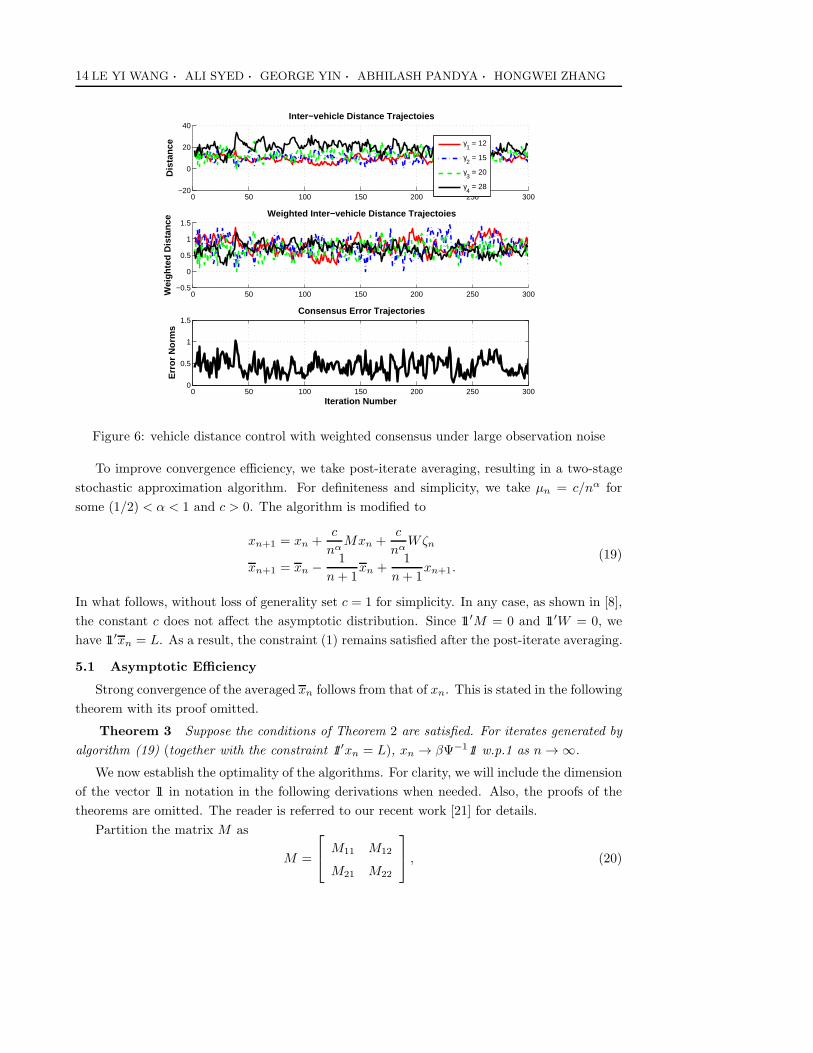
fluctuations. For example, for the same system as in Example 2, if the noise standard deviation
is increased from 1 to 20, its state trajectories demonstrate large variations, as shown in Figure
6.
14 LE YI WANG · ALI SYED · GEORGE YIN · ABHILASH PANDYA · HONGWEI ZHANG
0 50 100 150 200 250 300−20
0
20
40
Dis
tanc
e
Inter−vehicle Distance Trajectoies
γ1 = 12
γ2 = 15
γ3 = 20
γ4 = 28
0 50 100 150 200 250 300−0.5
0
0.5
1
1.5Weighted Inter−vehicle Distance Trajectoies
Wei
ghte
d D
ista
nce
0 50 100 150 200 250 3000
0.5
1
1.5Consensus Error Trajectories
Err
or N
orm
s
Iteration Number
Figure 6: vehicle distance control with weighted consensus under large observation noise
To improve convergence efficiency, we take post-iterate averaging, resulting in a two-stage
stochastic approximation algorithm. For definiteness and simplicity, we take µn = c/nα for
some (1/2) < α < 1 and c > 0. The algorithm is modified to
xn+1 = xn +c
nαMxn +
c
nαWζn
xn+1 = xn − 1
n+ 1xn +
1
n+ 1xn+1.
(19)
In what follows, without loss of generality set c = 1 for simplicity. In any case, as shown in [8],
the constant c does not affect the asymptotic distribution. Since 11′M = 0 and 11′W = 0, we
have 11′xn = L. As a result, the constraint (1) remains satisfied after the post-iterate averaging.
5.1 Asymptotic Efficiency
Strong convergence of the averaged xn follows from that of xn. This is stated in the following
theorem with its proof omitted.
Theorem 3 Suppose the conditions of Theorem 2 are satisfied. For iterates generated by
algorithm (19) (together with the constraint 11′xn = L), xn → βΨ−111 w.p.1 as n → ∞.
We now establish the optimality of the algorithms. For clarity, we will include the dimension
of the vector 11 in notation in the following derivations when needed. Also, the proofs of the
theorems are omitted. The reader is referred to our recent work [21] for details.
Partition the matrix M as
M =
M11 M12
M21 M22
, (20)

Control of Vehicle Platoons for Highway Safety and Efficient Utility 15
where M11 ∈ R(n−1)×(n−1), M12 ∈ R
(n−1)×1, M21 ∈ R(n−1)×1, and M22 ∈ R
1×1. Accordingly,
we also partition xn, xn, and W as
xn =
xn
xrn
; xn =
xn
xrn
; W =
W
W1
, (21)
respectively, with compatible dimensions with those of M .
Lemma 4 Under Assumption A0, M11 is full rank.
This result indicates that we can concentrate on r− 1 components of xn. We can show that
the asymptotic rate of convergence is independent of the choice of the r− 1 state variables. To
study the rates of convergence of xn, without loss of generality we need only examine that of
xn. It follows that
xn+1 = xn + µn(M11xn +M12xrn + W ζn)
= xn + µn(Mxn + Wζn),
xn+1 = xn − 1
n+ 1xn +
1
n+ 1xn+1,
(22)
where
M = M11 −M1211′r−1.
Note that the noise is now reduced also to W ζn, which is r− 1 dimensional but is a function of
ls dimensional link noise ζn.
Let D = Ir−1 + 11r−111′r−1.
Lemma 5 Under Assumption A0, M = M11D and is full rank.
For convergence speed analysis, let en = xn − βΨ−111n. Decompose en = [e′n, ern]
′.
Theorem 6 Suppose that {ζn} is a sequence of i.i.d. random variables with mean zero
and covariance Eζnζ′n = Σ. Under Assumption A0, the weighted consensus errors en satisfies
that√nen converges in distribution to a normal random variable with mean 0 and covariance
given by
M−1WΣW ′(M−1)′.
Note that the above result does not require any distributional information on the noise
{ε(k)} other than the zero mean and finite second moments. We now state the optimality of
the algorithm when the density function is smooth.
Theorem 7 Suppose that the noise {ζn} is a sequence of i.i.d. noise with a density f(·)that is continuously differentiable. Then the recursive sequence xn is asymptotically efficient in
the sense of the Cramer-Rao lower bound on Ee′nen being asymptotically attained,
nEe′nen → tr(M−1WΣW ′(M−1)′). (23)
The convergence speed and optimality of en is directly related to these of en.

16 LE YI WANG · ALI SYED · GEORGE YIN · ABHILASH PANDYA · HONGWEI ZHANG
Corollary 8 Under the conditions of Theorem 7, the sequence {xn} is asymptotically
efficient in the sense of the Cramer-Rao lower bound on Ee′nen being asymptotically attained.
The asymptotically optimal convergence speed is
nEe′nen → tr(DM−1WΣW ′(M−1)′) (24)
where D = Ir−1 + 11r−111′r−1.
Example 3 We now use the system in Example 2 to illustrate the effectiveness of post-
iterate averaging. Suppose that the link observation noises are i.i.d sequences of Gaussian noises
of mean zero and standard deviation 20. Now, the consensus control is expanded with post-
iterate averaging. Figure 7 shows the distance trajectories. The distance distributions converge
to the weighted consensus faster with much less fluctuations.
0 50 100 150 200 250 3000
10
20
30
Dis
tanc
e
Inter−vehicle Distance Trajectoies
γ1 = 12
γ2 = 15
γ3 = 20
γ4 = 28
0 50 100 150 200 250 3000
0.5
1Weighted Inter−vehicle Distance Trajectoies
Wei
ghte
d D
ista
nce
0 50 100 150 200 250 3000
0.2
0.4
0.6
0.8Consensus Error Trajectories
Err
or N
orm
s
Iteration Number
Figure 7: vehicle distance control with post-iterate averaging on weighted consensus algorithms
6 Network Topology and Platoon Control Performance
We investigate now the benefits of using communication systems to enhance platoon control.
In a sensor-based information network topology, we assume that the vehicles are equipped with
front and rear distance sensors, but control their front distances only. On the other hand, if
wireless communications are allowed, inter-vehicle information flows can be further expanded.
From the previous analysis, as long as the information topology is connected, convergence of
consensus control can be achieved. the main difference is the speed of convergence, which is
essential for system robustness, disturbance attenuation, and platoon re-configuration.
Example 4 This example compares the two types of information network topologies. The
platoon contains a lead vehicle and 5 other vehicles. In the sensor-based topology, vehicle j
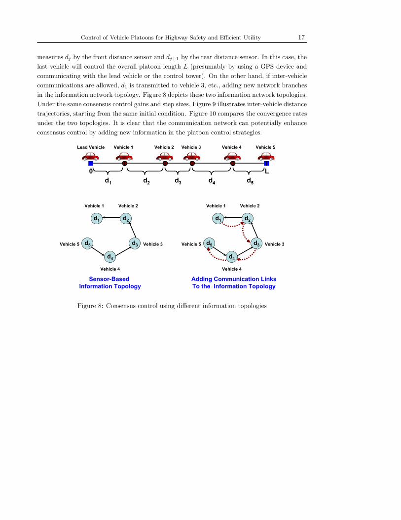
Control of Vehicle Platoons for Highway Safety and Efficient Utility 17
measures dj by the front distance sensor and dj+1 by the rear distance sensor. In this case, the
last vehicle will control the overall platoon length L (presumably by using a GPS device and
communicating with the lead vehicle or the control tower). On the other hand, if inter-vehicle
communications are allowed, d1 is transmitted to vehicle 3, etc., adding new network branches
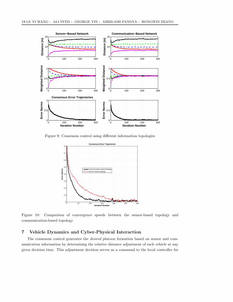
in the information network topology. Figure 8 depicts these two information network topologies.
Under the same consensus control gains and step sizes, Figure 9 illustrates inter-vehicle distance
trajectories, starting from the same initial condition. Figure 10 compares the convergence rates
under the two topologies. It is clear that the communication network can potentially enhance
consensus control by adding new information in the platoon control strategies.
0 L
d1 d2 d3 d4
Vehicle 1
d5
Vehicle 2 Vehicle 3 Vehicle 4 Vehicle 5Lead Vehicle
Vehicle 1 Vehicle 2
Sensor-Based
Information Topology
d1 d2
d3d5
d4
Vehicle 3
Vehicle 4
Vehicle 5
Vehicle 1 Vehicle 2
Adding Communication Links
To the Information Topology
d1 d2
d3d5
d4
Vehicle 3
Vehicle 4
Vehicle 5
Figure 8: Consensus control using different information topologies
18 LE YI WANG · ALI SYED · GEORGE YIN · ABHILASH PANDYA · HONGWEI ZHANG
0 100 200 3000
10
20Communication−Based Network
Dis
tanc
e (m
)
0 100 200 3000
0.5
1
Wei
ghte
d D
ista
nce
0 100 200 3000
0.5
1E
rror
Nor
ms
Iteration Number
0 100 200 3000
10
20Sensor−Based Network
Dis
tanc
e (m
)
0 100 200 3000
0.5
1
Wei
ghte
d D
ista
nce
0 100 200 3000
0.5
1Consensus Error Trajectories
Err
or N
orm
s
Iteration Number
Figure 9: Consensus control using different information topologies
0 50 100 150 200 250 3000
0.1
0.2
0.3
0.4
0.5
0.6
0.7
0.8Consensus Error Trajectories
Err
or N
orm
s
Iteration Number
Communication−based topologySensor−based topology
Figure 10: Comparison of convergence speeds between the sensor-based topology and
communication-based topology
7 Vehicle Dynamics and Cyber-Physical Interaction
The consensus control generates the desired platoon formation based on sensor and com-
munication information by determining the relative distance adjustment of each vehicle at any
given decision time. This adjustment decision serves as a command to the local controller for

Control of Vehicle Platoons for Highway Safety and Efficient Utility 19
execution. Due to vehicle dynamics and road/traffic conditions, execution of such control ac-
tions encounter standard performance limitations such as steady-state errors, overshoot, rising
time, delay, and other relevant performance measures. Inter-connection and interaction be-
tween information gathering and decision making at the higher level (cyber space) and vehicle
control (physical space) are illustrated in Fig. 11.
0 L
d1 d2 d3 d4
Vehicle 1
d5
Vehicle 2 Vehicle 3 Vehicle 4 Vehicle 5 Lead Vehicle
Vehicle 1 Vehicle 2
d1 d2
d3 d5
d4
Vehicle 3
Vehicle 4
Vehicle 5
Sensor and
Communications
Control
and Decision
Command to
vehicles
Vehicle dynamics
and control
Vehicle Controller
position, speed,
distance Command from
cyber space
Physical Space
Cyber Space
Figure 11: Cyber-physical inter-connection and interaction.
7.1 Vehicle Dynamics and Normalization
The dynamics of the jth vehicle follows the basic law
mj vj = Fj − L0j(vj) + ε0j (25)
where mj is the mass of the vehicle, Fj is the vehicle driving force (when it is positive) or
braking force (when it is negative), L0j(vj) is the modeled load force (which is known and can
be used in control action), and ε0j is the uncertainty term which captures modeling errors,
unknown factors on tires, roads, weather conditions, measurement noise, etc.
Normalization of (25) results in
vj =Fj
mj−
L0j(vj)
mj+
ε0jmj
= uj − Lj(vj) + εj
= wj + εj .
Here, uj = Fj/mj is the control variable, Lj(vj) = L0j(vj)/mj is the normalized drag, εj =
ε0j/mj is the normalized uncertainty, and wj = uj − Lj(vj) is a linearized control input.
20 LE YI WANG · ALI SYED · GEORGE YIN · ABHILASH PANDYA · HONGWEI ZHANG
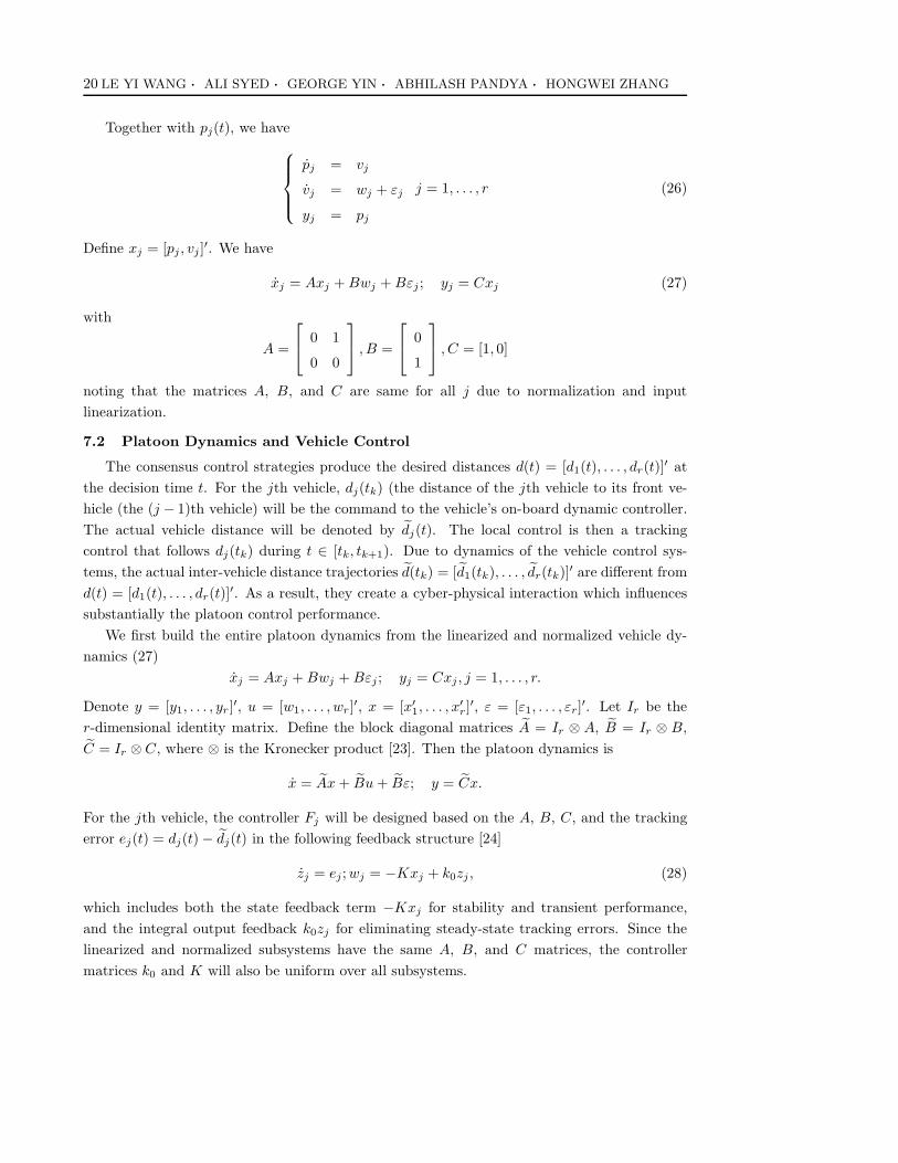
Together with pj(t), we have
pj = vj
vj = wj + εj
yj = pj
j = 1, . . . , r (26)
Define xj = [pj , vj ]′. We have
xj = Axj +Bwj +Bεj ; yj = Cxj (27)
with
A =
0 1
0 0
, B =
0
1
, C = [1, 0]
noting that the matrices A, B, and C are same for all j due to normalization and input
linearization.
7.2 Platoon Dynamics and Vehicle Control
The consensus control strategies produce the desired distances d(t) = [d1(t), . . . , dr(t)]′ at
the decision time t. For the jth vehicle, dj(tk) (the distance of the jth vehicle to its front ve-
hicle (the (j − 1)th vehicle) will be the command to the vehicle’s on-board dynamic controller.
The actual vehicle distance will be denoted by dj(t). The local control is then a tracking
control that follows dj(tk) during t ∈ [tk, tk+1). Due to dynamics of the vehicle control sys-
tems, the actual inter-vehicle distance trajectories d(tk) = [d1(tk), . . . , dr(tk)]′ are different from
d(t) = [d1(t), . . . , dr(t)]′. As a result, they create a cyber-physical interaction which influences
substantially the platoon control performance.
We first build the entire platoon dynamics from the linearized and normalized vehicle dy-
namics (27)
xj = Axj +Bwj +Bεj ; yj = Cxj , j = 1, . . . , r.
Denote y = [y1, . . . , yr]′, u = [w1, . . . , wr]
′, x = [x′1, . . . , x
′r]
′, ε = [ε1, . . . , εr]′. Let Ir be the
r-dimensional identity matrix. Define the block diagonal matrices A = Ir ⊗ A, B = Ir ⊗ B,
C = Ir ⊗ C, where ⊗ is the Kronecker product [23]. Then the platoon dynamics is
x = Ax+ Bu+ Bε; y = Cx.
For the jth vehicle, the controller Fj will be designed based on the A, B, C, and the tracking
error ej(t) = dj(t)− dj(t) in the following feedback structure [24]
zj = ej ;wj = −Kxj + k0zj , (28)
which includes both the state feedback term −Kxj for stability and transient performance,
and the integral output feedback k0zj for eliminating steady-state tracking errors. Since the
linearized and normalized subsystems have the same A, B, and C matrices, the controller
matrices k0 and K will also be uniform over all subsystems.

Control of Vehicle Platoons for Highway Safety and Efficient Utility 21
By denoting z = [z′1, . . . , z′r]
′, e = [e1, . . . , er]′, K = Ir ⊗K, the controller for the platoon is
z = e;u = −Kx+ k0z.
Note that d1 = p1 − p0, . . ., dr = pr − pr−1, where the leading vehicle’s position p0 is external
to the system as the time-varying reference to the platoon. Then, e1 = d1 − (p1 − p0), . . .,
er = dr − (pr − pr−1). The platoon dynamics is represented by
z = e
x = Ax+ Bu+ Bε
u = −Kx+ k0z
e = −SCx+B1p0 + d
(29)
where
S =
1 0 · · · 0 0
−1 1 · · · 0 0...
...
0 0 · · · −1 1
;B1 =
1
0...
0
.
7.3 Platoon Stability
Platoon stability has been studied as a string stability when consecutive vehicles use only
the immediate distance information in its cruise control, see [11, 18] and the references therein.
Platoon stability is not a trivial issue, depending on how local systems are controlled. Here,
we study platoon stability using a unified local control structure by input linearization and
scaling, a coordination of desired distances by the weighted and constrained consensus control,
and a state-feedback-plus-integral-output-feedback structure for local feedback. The advantage
of these structures is that it makes stability analysis simpler.
To illustrate platoon stability, we note that K = [k1, k2]. This implies K = Ir ⊗ [k1, k2].
Hence, (29) is
z = e
x = Ax+ Bu+ Bε
u = −(Ir ⊗ [k1, k2])x+ k0z
e = −SCx+B1p0 + d
(30)
Theorem 9 The jth subsystem has the closed-loop system zj
xj
=
0 −C
Bk0 A−BK
zj
xj
+B0pj−1 +B0dj +
0
B
εj,
where B0 = [1, 0, 0]′.
The closed-loop system for the entire platoon is z
x
=
0 −SC
Bk0 A− B(Ir ⊗ [k1, k2])
z
x
+
B1
0
p0 +
Ir
0
d+
0
B
ε.

22 LE YI WANG · ALI SYED · GEORGE YIN · ABHILASH PANDYA · HONGWEI ZHANG
Proof: The controller for the jth vehicle is
zj = ej = k0(dj − (Cxj − pj−1));wj = −[k1, k2]xj + k0zj. (31)
pj−1 is an external signal to the jth vehicle. Combined with the vehicle dynamics (27), the
closed-loop system is
zj = −k0Cxj + k0(pj−1 + dj)
xj = Axj +Bwj = (A−BK)xj + k0Bzj +Bεj .
k0, k1, k2 are to be designed such that the closed-loop system is stable. Hence, the closed-loop
system is zj
xj
=
0 −C
Bk0 A−BK
zj
xj
+B0pj−1 +B0dj +
0
B
εj. (32)
From (30), the closed-loop system for the platoon is
z = −SCx+B1p0 + d
x = Ax+ B(k0z − (Ir ⊗ [k1, k2])x) + Bε(33)
or compactly z
x
=
0 −SC
Bk0 A− B(Ir ⊗ [k1, k2])
z
x
+
B1
0
p0 +
Ir
0
d+
0
B
ε.
�
k0, k1, k2 are designed to achieve local stability. From
A =
0 1
0 0
, B =
0
1
, C = [1, 0],
we have
φ =
0 −C
Bk0 A−BK
=
0 −1 0
0 0 1
k0 −k1 −k2
. (34)
The subsystem is stable if all eigenvalues of φ are in the left-half plane. The characteristic
polynomial of φ is λ3+k2λ2+k1λ+k0. Apparently, any desired pole assignment can be realized.
For example, if the desired characteristis polynomial is (λ + p)3 = λ3 + 3pλ2 + 3p2λ + p3, for
some p > 0, then k0 = p3, k1 = 3p2, k2 = 3p will be the designed control parameters.
We now establish stability of the entire platoon. Stability of the entire platoon is determined
by the eigenvalues of
Φ =
0 −SC
Bk0 A− B(Ir ⊗ [k1, k2])
. (35)

Control of Vehicle Platoons for Highway Safety and Efficient Utility 23
Theorem 10 The eigenvalues of Φ are the same as the eigenvalues of φ, but repeated r
times each. As a result, if the subsystems are designed to be stable, then the entire platoon is
stable.
Proof: In consideration of the local control nature, we first re-arrange (30) into a subsystem
structure. Let ξj = [zj, x′j ]
′. Then the jth closed-loop system is
ξj = φξj +B0pj−1 +B0dj +
0
B
εj
pj = [0, C]ξj
j = 1, . . . , r.
For stability analysis, we ignore p0, dj , and εj, arriving at
ξj = φξj +B0pj−1
pj = [0, C]ξjj = 1, . . . , r.
Consequently, the platoon closed-loop system is
ξ1...
ξr
=
φ 0 · · · 0 0
B0[0, C] φ · · · 0 0...
...
0 0 · · · B0[0, C] φ
ξ1...
ξr
. (36)
Since this is a block diagonal matrix, its eigenvalues are the collection of the eigenvalues of its
diagonal blocks, which are the eigenvalues of φ. This re-arrangement of the platoon closed-loop
system does not change the eigenvalues of Φ. This completes the proof.
�
Example 5 Select k0 = 1, k1 = 2, k2 = 2. Then
φ =
0 −C
Bk0 A−BK
=
0 −1 0
0 0 1
1 −2 −2
.
Its eigenvalues are −1, −0.5± j0.866. Suppose that the platoon has r = 3. It can be verified
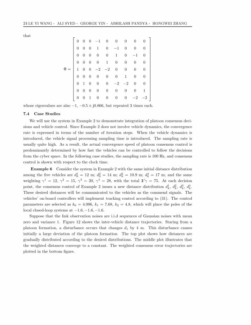
24 LE YI WANG · ALI SYED · GEORGE YIN · ABHILASH PANDYA · HONGWEI ZHANG
that
Φ =
0 0 0 −1 0 0 0 0 0
0 0 0 1 0 −1 0 0 0
0 0 0 0 0 1 0 −1 0
0 0 0 0 1 0 0 0 0
1 0 0 −2 −2 0 0 0 0
0 0 0 0 0 0 1 0 0
0 1 0 0 0 −2 −2 0 0
0 0 0 0 0 0 0 0 1
0 0 1 0 0 0 0 −2 −2
whose eigenvalues are also −1, −0.5± j0.866, but repeated 3 times each.
7.4 Case Studies
We will use the system in Example 2 to demonstrate integration of platoon consensus deci-
sions and vehicle control. Since Example 2 does not involve vehicle dynamics, the convergence
rate is expressed in terms of the number of iteration steps. When the vehicle dynamics is
introduced, the vehicle signal processing sampling time is introduced. The sampling rate is
usually quite high. As a result, the actual convergence speed of platoon consensus control is
predominantly determined by how fast the vehicles can be controlled to follow the decisions
from the cyber space. In the following case studies, the sampling rate is 100 Hz, and consensus
control is shown with respect to the clock time.
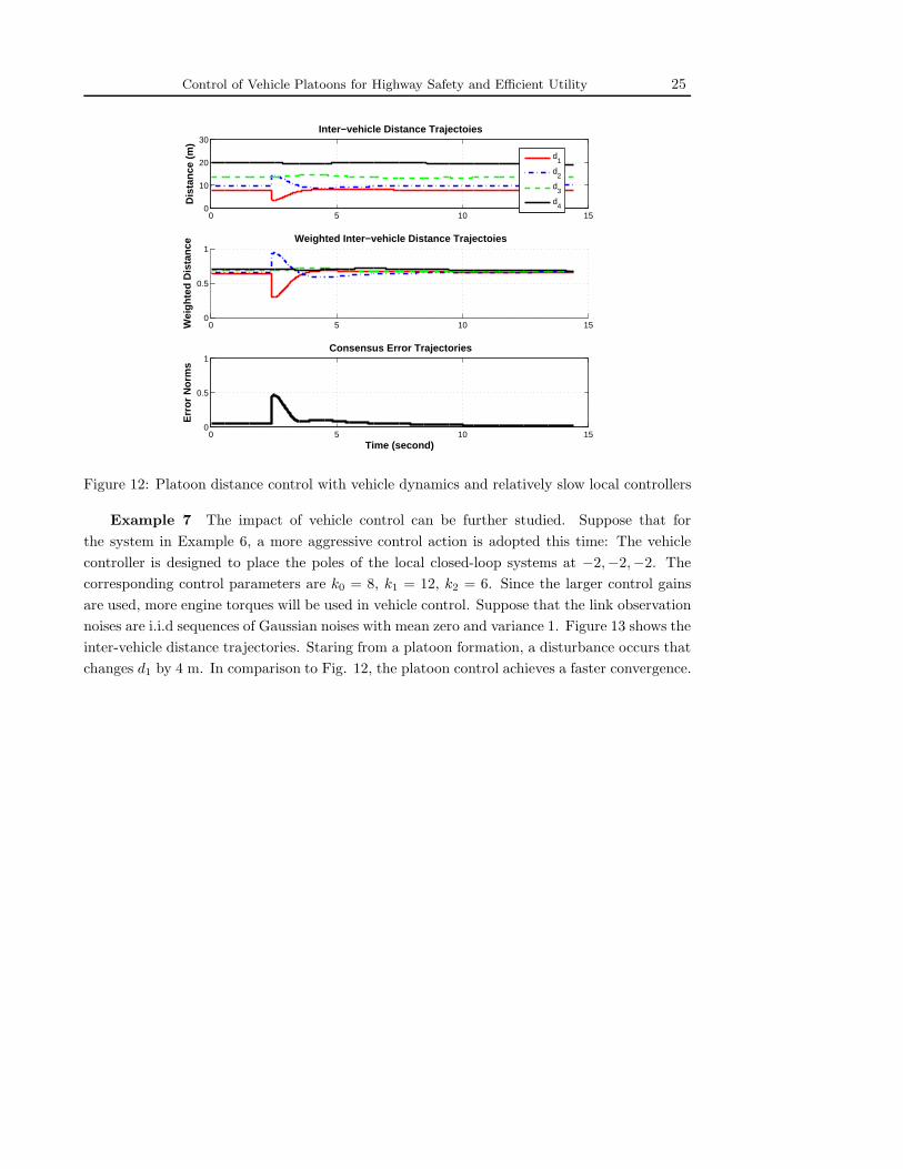
Example 6 Consider the system in Example 2 with the same initial distance distribution
among the five vehicles are d10 = 12 m; d20 = 14 m; d30 = 10.9 m; d40 = 17 m; and the same
weighting γ1 = 12, γ2 = 15, γ3 = 20, γ4 = 28, with the total 11′γ = 75. At each decision
point, the consensus control of Example 2 issues a new distance distribution d1k, d2k, d
3k, d
4k.
These desired distances will be communicated to the vehicles as the commend signals. The
vehicles’ on-board controllers will implement tracking control according to (31). The control
parameters are selected as k0 = 4.096, k1 = 7.68, k2 = 4.8, which will place the poles of the
local closed-loop systems at −1.6,−1.6,−1.6.
Suppose that the link observation noises are i.i.d sequences of Gaussian noises with mean
zero and variance 1. Figure 12 shows the inter-vehicle distance trajectories. Staring from a
platoon formation, a disturbance occurs that changes d1 by 4 m. This disturbance causes
initially a large deviation of the platoon formation. The top plot shows how distances are
gradually distributed according to the desired distributions. The middle plot illustrates that
the weighted distances converge to a constant. The weighted consensus error trajectories are
plotted in the bottom figure.
Control of Vehicle Platoons for Highway Safety and Efficient Utility 25
0 5 10 150
10
20
30
Dis
tanc
e (m
)
Inter−vehicle Distance Trajectoies
d1
d2
d3
d4
0 5 10 150
0.5
1Weighted Inter−vehicle Distance Trajectoies
Wei
ghte
d D
ista
nce
0 5 10 150
0.5
1Consensus Error Trajectories
Err
or N
orm
s
Time (second)
Figure 12: Platoon distance control with vehicle dynamics and relatively slow local controllers
Example 7 The impact of vehicle control can be further studied. Suppose that for
the system in Example 6, a more aggressive control action is adopted this time: The vehicle
controller is designed to place the poles of the local closed-loop systems at −2,−2,−2. The
corresponding control parameters are k0 = 8, k1 = 12, k2 = 6. Since the larger control gains
are used, more engine torques will be used in vehicle control. Suppose that the link observation
noises are i.i.d sequences of Gaussian noises with mean zero and variance 1. Figure 13 shows the
inter-vehicle distance trajectories. Staring from a platoon formation, a disturbance occurs that
changes d1 by 4 m. In comparison to Fig. 12, the platoon control achieves a faster convergence.

26 LE YI WANG · ALI SYED · GEORGE YIN · ABHILASH PANDYA · HONGWEI ZHANG
0 5 10 150
10
20
30
Dis
tanc
e (m
)
Inter−vehicle Distance Trajectoies
d1
d2
d3
d4
0 5 10 150
0.5
1Weighted Inter−vehicle Distance Trajectoies
Wei
ghte
d D
ista
nce
0 5 10 150
0.5
1Consensus Error Trajectories
Err
or N
orm
s
Time (second)
Figure 13: Platoon distance control with vehicle dynamics and more aggressive local controllers
7.5 Remarks on Platoon Coordination with Safety Constraints
Safety concern is the highest priority in highway platoon control. As a result, it is important
that safety features are incorporated into platoon control algorithms. In this section, we consider
the case of safety boundary constraints on inter-vehicle distances that override other control
actions such as consensus algorithms or vehicle local control actions.
Suppose that inter-vehicle distance between the ith and (i− 1)th vehicles must be bounded
below by dimin for safety and above by dimax for highway utility. For example, 3 m for low speed
drive and 5 m for highway cruise are typically used as a safety lower bound in several commercial
vehicle safety systems. Mathematically, these constraints amount to a constraint set Ξ, which
is assumed to be closed, on the state xn. Although the constraint set typically changes with
operating conditions, such as vehicle speeds, due to similarity in their treatment we will focus
on the case that Ξ is given and fixed. In the case of box constraints (i.e., the constrained set
being the product of closed intervals), Ξ = [d1min, d1max] × · · · × [drmin, d
rmax]. Incorporating the
constraint set Ξ into the platoon control involves two levels.
1. Platoon Coordination. At the cyber space, the consensus updating algorithm (9)
xn+1 = xn + µn(Mxn +Wζn)
is modified to an updating algorithm with projection.
xn+1 = ΠΞ(xn + µn(Mxn +Wζn)) (37)
Control of Vehicle Platoons for Highway Safety and Efficient Utility 27
where the projection operator ΠΞ is defined as
Π(x) =
x, x ∈ Ξ,
x∗, x 6∈ Ξ.
Here x∗ is a pre-selected interior point of Ξ. In other words, if the constraint set Ξ is
violated, the interative consensus algorithm will be reset to the point x∗.
Note that in the setup of such a box constrained algorithm, all the analysis presented
before goes through. Even more complex constrained sets can be incorporated. More
details on the analysis of such algorithms can be found in [8].
2. Vehicle Control. At the vehicle level, the on-board vehicle control system for the ith
vehicle will manipulate its control signal such that if the distance di reaches its lower
bound dimin, its control will be confined to the set that can only increase di. We will
use an example to demonstrate this added feature. This control modification renders a
nonlinear feedback structure to the vehicle controller.
8 Concluding Remarks
Platoon control strategies and algorithms introduced in this paper represent a new frame-
work for intelligent highway transportation systems. As a first step in this direction, this paper
is focused on establishing the key structure of the framework, the main algorithms, and fun-
damental interactions between the consensus decision on the cyber space and vehicle control
in the physical space. As such the system models are of basic and representative types, rather
than detailed physical systems. For the same token, there are many important and intriguing
issues left open for further exploration.
First, detailed vehicle dynamics will be of interests. Second, communication systems have
experienced great advancement in recent years. For vehicle applications, some communication
protocols, such as DSRC, have emerged as potential standards for V2V and V2I communi-
cations. As such, it will be important to include detailed features of these protocols in this
framework such that relevant evaluations can be conducted on the viability, advantages, and
limitations of our framework. Third, enhanced vehicle safety considerations introduce many
nonlinear constraints in vehicle control. Integrated consensus decision and vehicle control under
nonlinear constraints are of essential importance. These directions will be pursued in our future
studies.
References
[1] S.B. Choi and J.K. Hedrick, Vehicle longitudinal control using an adaptive observer for automated highway
systems, Proc. of ACC, Seattle, 1995.
28 LE YI WANG · ALI SYED · GEORGE YIN · ABHILASH PANDYA · HONGWEI ZHANG
[2] J. Cortes and F. Bullo, Coordination and geometric optimization via distributed dynamical systems, SIAM
J. Control Optim., no. 5, pp. 1543-1574, May 2005.
[3] J.K. Hedrick, D. McMahon, D. Swaroop, Vehicle modeling and control for automated highway systems,
PATH Research Report, UCB-ITS-PRR-93-24, 1993.
[4] M. Huang and J.H. Manton. Coordination and consensus of networked agents with noisy measurements:
stochastic algorithms and asymptotic behavior,” SIAM J. Control Optim., vol. 48, no. 1, pp. 134-161, 2009.
[5] M. Huang, S. Dey, G.N. Nair, J.H. Manton, Stochastic consensus over noisy networks with Markovian and
arbitrary switches, Automatica, 46 (2010), 1571–1583.
[6] A. Jadbabaie, J. Lin, and A. S. Morse. Coordination of groups of mobile autonomous agents using nearest
neighbor rules, IEEE Trans. Automat. Contr., vol. 48, pp. 988-1000, June 2003.
[7] S. Karlin and H.M. Taylor, A First Course in Stochastic Processes, 2nd ed., Academic Press, New York,
NY, 1975.
[8] H.J. Kushner and G. Yin, Stochastic Approximation Algorithms and Applications, Springer-Verlag, New
York, 2nd Ed., 2003.
[9] T. Li and J. F. Zhang, Consensus conditions of multi-agent systems with time-varying topologies and
stochastic communication noises, IEEE Trans. on Automatic Control, Vol.55, No.9, 2043-2057, 2010.
[10] Tao Li, Minyue Fu, Lihua Xie and Ji-Feng Zhang, Distributed consensus with limited communication data
rate, IEEE Trans. on Automatic Control, Vol.56, No.2, 279-292, 2011.
[11] C Y Liang and Huei Peng, String stability analysis of adaptive cruise controlled vehicles, JSME International
Journal Series C, Volume: 43, Issue: 3, pp. 671?77, 2000.
[12] L. Moreau, Stability of multiagent systems with time- dependent communication links, IEEE Trans. Autom.
Control, vol. 50, no. 2, pp. 169-182, Feb. 2005.
[13] M.B. Nelson and R.Z. Khasminskii, Stochastic Approximation and Recursive Estimation, Amer. Math.
Soc., Providence, RI, 1976.
[14] B. T. Polyak, New method of stochastic approximation type, Automation Remote Control 7 (1991), 937–
946.
[15] R. Rajamani, H.S. Tan, B. Law and W.B. Zhang, Demonstration of Integrated Lateral and Longitudinal
Control for the Operation of Automated Vehicles in Platoons, IEEE Transactions on Control Systems
Technology, Vol. 8, No. 4, pp. 695-708, July 2000.
[16] W. Ren and R.W. Beard. Consensus seeking in multiagent systems under dynamically changing interaction
topologies, IEEE Trans. Automat. Control, vol. 50, no. 5, pp. 655-661, 2005.
[17] D. Ruppert, Stochastic approximation, in Handbook in Sequential Analysis, B. K. Ghosh and P. K. Sen,
eds., Marcel Dekker, New York, 1991, 503-529.
[18] D. Swaroop and J. Hedrick, String Stability of Interconnected Systems,?IEEE Transactions on Automatic
Control? Vol. 41, No. 3, pp. 349-357, Mar. 1996.
[19] Le Yi Wang and George Yin, Weighted and Constrained Consensus Control with Performance for Robust
Distributed UAV Deployments with Dynamic Information Networks, in Recent advances in UAV control
systems, ed. G. Yin and L.Y. Wang, 2012.
[20] Le Yi Wang, Caisheng Wang, George Yin, Weighted and Constrained Consensus for Distributed Power
Flow Control, PMAPS 2012, Istanbul, Turkey, June 10-14, 2012.
[21] G. Yin, Y. Sun, and L.Y. Wang, Asymptotic properties of consensus-type algorithms for networked systems
with regime-switching topologies, Automatica, 47 (2011) 1366–1378.
[22] G. Yin, Le Yi Wang, Yu Sun: Stochastic Recursive Algorithms for Networked Systems with Delay and
Random Switching: Multiscale Formulations and Asymptotic Properties, Multiscale Modeling & Simulation
9(3): 1087-1112, 2011.
[23] R.A. Horn and C.R. Johnson, Matrix Analysis, Cambridge University Press, 1985.
[24] B.C. Kuo, F. Golnaraghi,, Automatic Control Systems, 8th Ed., John Wiley & Sons, 2002.