control oriented modeling of the dynamics in a catalytic ... · dynamics in a catalytic converter...
TRANSCRIPT
Control Oriented Modeling of the
Dynamics in a Catalytic Converter
Master’s thesis
performed in Vehicular Systems
byJenny Johansson and Mikaela Waller
Reg nr: LiTH-ISY-EX–05/3707–SE
23rd September 2005

Control Oriented Modeling of the
Dynamics in a Catalytic Converter
Master’s thesis
performed in Vehicular Systems,Dept. of Electrical Engineering
at Linkopings universitet
by Jenny Johansson and Mikaela Waller
Reg nr: LiTH-ISY-EX–05/3707–SE
Supervisor: Per Oberg
ISYRichard Backman
GM Powertrain Sweden
Examiner: Associate Professor Lars Eriksson
Linkopings Universitet
Linkoping, 23rd September 2005

Avdelning, Institution
Division, DepartmentDatum
Date
Sprak
Language
� Svenska/Swedish
� Engelska/English
�
Rapporttyp
Report category
� Licentiatavhandling
� Examensarbete
� C-uppsats
� D-uppsats
� Ovrig rapport
�
URL for elektronisk version
ISBN
ISRN
Serietitel och serienummer
Title of series, numberingISSN
Titel
Title
Forfattare
Author
Sammanfattning
Abstract
Nyckelord
Keywords
The legal amount of emissions that vehicles with spark ignited enginesare allowed to produce are steadily reduced over time. To meet futureemission requirements it is desirable to make the catalytic converterwork in a more efficient way. One way to do this is to control the air-fuel-ratio according to the oxygen storage level in the converter, insteadof, as is done today, always trying to keep it close to stoichiometric.The oxygen storage level cannot be measured by a sensor. Hence, amodel describing the dynamic behaviors of the converter is needed toobserve this level. Three such models have been examined, validated,and compared.
Two of these models have been implemented in Matlab/Simulink andadapted to measurements from an experimental setup. Finally, one ofthe models was chosen to be incorporated in an extended Kalman filter(EKF), in order to make it possible to observe the oxygen storage levelonline.
The model that shows best potential needs further work, and theEKF is working with flaws, but overall the results are promising.
Vehicular Systems,Dept. of Electrical Engineering581 83 Linkoping
23rd September 2005
—
LITH-ISY-EX–05/3707–SE
—
http://www.vehicular.isy.liu.sehttp://www.ep.liu.se/exjobb/isy/2005/3707/
Control Oriented Modeling of the Dynamics in a Catalytic Converter
Modellering av dynamiken i en katalysator med avseende pa reglering
Jenny Johansson and Mikaela Waller
××
catalytic converter, TWC, oxygen storage, lambda, observer, EKF,modeling, simulation

Abstract
The legal amount of emissions that vehicles with spark ignited enginesare allowed to produce are steadily reduced over time. To meet futureemission requirements it is desirable to make the catalytic converterwork in a more efficient way. One way to do this is to control the air-fuel-ratio according to the oxygen storage level in the converter, insteadof, as is done today, always trying to keep it close to stoichiometric.The oxygen storage level cannot be measured by a sensor. Hence, amodel describing the dynamic behaviors of the converter is needed toobserve this level. Three such models have been examined, validated,and compared.
Two of these models have been implemented in Matlab/Simulinkand adapted to measurements from an experimental setup. Finally, oneof the models was chosen to be incorporated in an extended Kalmanfilter (EKF), in order to make it possible to observe the oxygen storagelevel online.
The model that shows best potential needs further work, and theEKF is working with flaws, but overall the results are promising.
Keywords: catalytic converter, TWC, oxygen storage, lambda, ob-server, EKF, modeling, simulation
v

vi
Sammanfattning
Avgasmangden som bensindrivna fordon tillats slappa ut minskas helatiden. Ett satt att mota framtida krav, ar att forbattra katalysatornseffektivitet. For att gora detta kan luft-bransle-forhallandet reglerasmed avseende pa syrelagringen i katalysatorn, istallet for som idag, re-glera mot stokiometriskt blandningsforhallande. Eftersom syrelagrin-gen inte gar att mata med en givare behovs en modell som beskriverkatalysatorns dynamiska egenskaper. Tre sadana modeller har un-dersokts, utvarderats och jamforts.
Tva av modellerna har implementerats i Matlab/Simulink och an-passats till matningar fran en experimentuppstallning. For att kunnaobservera syrelagringen online valdes slutligen en av modellerna ut, ochimplementerades i ett Extended Kalman filter.
Ytterligare arbete behover laggas ner pa den mest lovande mod-ellen, och detsamma galler for Kalmanfiltret, men pa sikt forvantasresultaten kunna bli bra.
Nyckelord: katalysator, TWC, syrelagring, lambda, observator, EKF,modellering, simulering
vii

viii

Acknowledgement
We would like to thank our supervisor Per Oberg at Fordonssystem forall his help and rewarding discussions. We would also like to thankour examiner Lars Eriksson for interesting discussions and always be-ing able to raise new questions. Additionally this thesis would nothave existed without the help and support from Richard Backman, oursupervisor at GM Powertrain Sweden.
Very special thanks go to Dr. Theophil Auckenthaler. Withoutyour help, explanations, and answers our work would have been somuch harder.
Thank you Martin Gunnarsson, for helping us in the engine labora-tory, Per Andersson and the rest of the staff at Fordonssystem for thesupport, as well as creating the great atmosphere at Fordonssystem.
Furthermore we would like to thank Staffan and Birgitta, who havebeen of great help in many ways. We are especially thankful for yourpatience with the endless discussions about catalytic converters.
The last thanks go to our roommates Claes and Eric. Perhaps wedid not hit the paper basket as often as you, but our mischiefs weredefinitely more entertaining.
ix

x

Notation
Nomenclature
Variable Unit DescriptionA s−1 pre-exponential factorAgeo m2/m3 specific geometric catalyst surfaceAλst...Fλst V,- coefficients in the switch-type λ-sensor modelCi m/s convection mass transfer coefficient of iDchan m diameter gas channelDTWC m catalytic converter diameterE kJ/mol activation energyKd - constant of proportionalityKr - constant of proportionalityKλ - constant of proportionalityKψ - constant of proportionalityLTWC m TWC lengthSC mol/m3 storage capacityT K temperatureU V voltageVTWC m3 catalytic converter volume
V m3/s volumetric flowa1...a5 - coefficients in the polynomial describing N(φ)aηcomb
- coefficient in the exhaust gas modelbηcomb
1/K coefficient in the exhaust gas modelbi - triangular basis functionsc mol/m3 concentrationcp J/kg*K specific heat capacity (gas phase)cs J/kg*K specific heat capacity (solid phase)f1,2..n - tuning parametersfL - function for lean inputfR - function for rich inputg(ζ) - function in Model Bk 1/s reaction rate coefficientkd - parameter in Model Bmf kg/s fuel mass flownc - number of discrete cellsr - reaction rateyi - mole fractions∆H J/mol reaction enthalpy∆Λ - post-catalyst AFR deviation from stoichiometric be-
fore the effect of the catalyst deactivation
xi
∆λ - λ− 1Σi - diffusion volumesα W/m2K heat-transfer coefficient TWC → exhaustαcat W/m2K heat-transfer coefficient TWC → ambientε - volume fraction of gas phaseζ - global fraction of oxygen storageηCO - number of sites occupied by COηcomb - inverse combustion efficiencyθ - occupancy fraction on noble metalλ - normalized air-fuel-ratioλs W/m*K heat conductivity solid phaseξ - local fraction of oxygen storageρs kg/m3 density solid phaseφ - oxygen storage levelφH2/CO - H2/CO ratioψ - reversible catalyst deactivation
Vectors and matrices
Variable Descriptionf dynamics function of state-space systemh measurement function of state-space systemu control vectorx state vectory measurement vectorv,w uncorrelated white noise processF system dynamics matrixH system measurement matrixI identity matrixK kalman gain matrixP covariance matrix of the estimate errorQ covariance matrix of process white noiseR covariance matrix of measurement white noiseΦ fundamental matrix
xii
Subscripts
Subscript Descriptionex excess of the species after a surface reaction has been
completedexh exhaustg gasin incoming variable to the converterout outgoing variable after the converterpost denotes the variable after the converterpre denotes the variable before the converters solidtp tail-pipeλst switch-type λ
Superscripts
Superscript Descriptionads adsorptionch channelox oxidationred reductionwc washcoat∗ vacant site in the catalytic converter
Abbreviations
AFR Air-Fuel-RatioFTP 75 American Federal Test ProcedureNEDC New European Driving CycleO, P, R Oxidants, Products and ReactantsROC Relative Oxygen coverage of CeriaTWC Three-Way catalytic Converter
Constants
Variable Value/Unit Descriptionℜ 8.31451 J/molK universal gas constant
xiii

xiv
Contents
Abstract v
Sammanfattning vii
Acknowledgement ix
Notation xi
1 Introduction 1
1.1 Background . . . . . . . . . . . . . . . . . . . . . . . . . 11.1.1 Regulations . . . . . . . . . . . . . . . . . . . . . 11.1.2 Catalytic converters . . . . . . . . . . . . . . . . 2
1.2 Purpose and method . . . . . . . . . . . . . . . . . . . . 31.3 Prerequisites . . . . . . . . . . . . . . . . . . . . . . . . 41.4 Thesis Outline . . . . . . . . . . . . . . . . . . . . . . . 4
2 Model Verification Method 7
2.1 Experimental setup . . . . . . . . . . . . . . . . . . . . . 72.2 Data . . . . . . . . . . . . . . . . . . . . . . . . . . . . 82.3 Model adaption strategy . . . . . . . . . . . . . . . . . . 92.4 Validation . . . . . . . . . . . . . . . . . . . . . . . . . . 9
3 Introduction to Emissions and Catalytic Converters 11
3.1 Combustion Engines and Emissions . . . . . . . . . . . . 113.2 The Catalytic Converter . . . . . . . . . . . . . . . . . . 123.3 Study of the dynamics . . . . . . . . . . . . . . . . . . 14
3.3.1 The sensors’ influence on the measurements . . . 143.3.2 Study of the measurements . . . . . . . . . . . . 16
4 Model A - A Storage Dominated Model with ... 19
4.1 Model . . . . . . . . . . . . . . . . . . . . . . . . . . . . 194.1.1 The oxygen storage state, φ . . . . . . . . . . . . 204.1.2 The reversible catalyst deactivation, ψ . . . . . . 214.1.3 Estimated ∆λ value after the catalytic converter 21
xv
4.2 Convert to switch type λ-values . . . . . . . . . . . . . . 214.3 Parameter Estimation . . . . . . . . . . . . . . . . . . . 22
4.3.1 Catalytic Converter Parameters . . . . . . . . . . 234.3.2 Exhaust Gas and Sensor Parameters . . . . . . . 244.3.3 Parameters adjusted to the age of the converter . 24
4.4 Discussion . . . . . . . . . . . . . . . . . . . . . . . . . . 244.4.1 The extension to switch-type λ-values . . . . . . 254.4.2 Validation . . . . . . . . . . . . . . . . . . . . . . 264.4.3 Results . . . . . . . . . . . . . . . . . . . . . . . 27
5 Model B - A Model Consisting of One Nonlinear... 31
5.1 Model . . . . . . . . . . . . . . . . . . . . . . . . . . . . 315.1.1 Model developement . . . . . . . . . . . . . . . . 315.1.2 The complete model . . . . . . . . . . . . . . . . 345.1.3 Model parameters and functions . . . . . . . . . 34
5.2 Parameter estimation . . . . . . . . . . . . . . . . . . . 355.3 Validation . . . . . . . . . . . . . . . . . . . . . . . . . . 36
6 Model C - A Simplified Physical... 39
6.1 Model . . . . . . . . . . . . . . . . . . . . . . . . . . . . 396.1.1 Exhaust gas model . . . . . . . . . . . . . . . . . 396.1.2 TWC model . . . . . . . . . . . . . . . . . . . . . 416.1.3 Switch-type λ-sensor model . . . . . . . . . . . . 45
6.2 Parameter estimation . . . . . . . . . . . . . . . . . . . 466.2.1 Simplifications and assumption . . . . . . . . . . 476.2.2 Estimation algorithm . . . . . . . . . . . . . . . 47
6.3 Validation . . . . . . . . . . . . . . . . . . . . . . . . . . 486.3.1 The first set . . . . . . . . . . . . . . . . . . . . . 496.3.2 The second set . . . . . . . . . . . . . . . . . . . 506.3.3 Number of cells . . . . . . . . . . . . . . . . . . . 516.3.4 Discussion . . . . . . . . . . . . . . . . . . . . . . 52
7 Model comparison 53
7.1 Accuracy of the models . . . . . . . . . . . . . . . . . . 537.2 Inputs and outputs . . . . . . . . . . . . . . . . . . . . . 547.3 Number of states and parameters . . . . . . . . . . . . . 557.4 Simulation speed . . . . . . . . . . . . . . . . . . . . . . 567.5 Extensibility . . . . . . . . . . . . . . . . . . . . . . . . 567.6 Final comparison . . . . . . . . . . . . . . . . . . . . . . 57
8 Extended Kalman filter 59
8.1 Introduction to EKF . . . . . . . . . . . . . . . . . . . . 598.1.1 Parameter identification . . . . . . . . . . . . . . 61
8.2 Implementation . . . . . . . . . . . . . . . . . . . . . . . 618.3 Tuning of the EKF . . . . . . . . . . . . . . . . . . . . . 62
xvi
8.4 Discussion and results . . . . . . . . . . . . . . . . . . . 638.4.1 Validation . . . . . . . . . . . . . . . . . . . . . . 638.4.2 Properties of the EKF . . . . . . . . . . . . . . . 64
9 Results and Discussion 67
10 Future work 69
References 71
A Chemical reactions 73
B Model A - Parameter Values 74
C Model C - Parameter Values 76
xvii

xviii
Chapter 1
Introduction
1.1 Background
Already in 1915, concerns were raised about the risk potential of auto-mobile pollutants, they were considered noisy, dangerous, and smelly.As a consequence the first regulation concerning emissions came in use1959 in California and since then the allowed emission levels have beenreduced. The automotive producers have a tough challenge. They donot only have to meet the emission requirements, they also want tosatisfy the customers’ power, fuel consumption and cost requirements,which often contradicts low emission rates.
1.1.1 Regulations
In 1968, US got the first federal standards during the Clean Air Act,mainly because the smog was becoming an increasing concern. The ini-tial targets were carbon monoxide and unburned hydrocarbons. A fewyears later, the adverse effect of oxides of nitrogen on the environmentwas recognized.
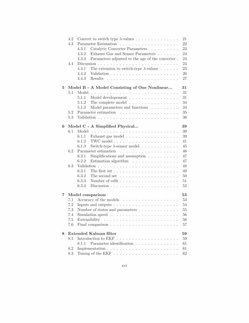
Since the first regulation, legislators all over the world have steadilyreduced the legal limits of emissions over time. This is demonstrated infigure 1.1, which shows how the emission regulations for petrol vehiclesin the US have changed over time.
The emission regulations are formulated as maximum values of emis-sions (measured in pollutant mass per distance traveled) from a vehiclefollowing a specified driving profile, called test cycle. There are differ-ent test cycles available. Two frequently used is the American FederalTest Procedure, FTP 75, and the New European Driving Cycle, NEDC.
1
2 Chapter 1. Introduction
1965 1970 1975 1980 1985 1990 1995 2000 20050
2
4
6
8
10
HC
and
NO
x [g
/mile
]
year
... CO −−− HC −.− NOx
1965 1970 1975 1980 1985 1990 1995 2000 20050
20
40
60
80
100
CO
[g/m
ile]
Figure 1.1: Legal limits of emissions in the US. Limits taken from [10].
1.1.2 Catalytic converters
The legal limits of emissions have forced the industry to accelerate thedevelopment of control systems and catalytic converters, but when thefirst regulation was introduced the only known way to reduce CO andHC was to lean the mixture of air and fuel. This put an end to increasesin specific power outputs for a few years. During the 1970s, the two-way catalytic converters (which oxidized both CO and HCs to waterand CO2) started to appear.
The most significant change in engine and catalytic converter tech-nology came with the recognition of the adverse effect of oxides ofnitrogen (NOx) on the environment. To deal with this ”new” prob-lem the combustion was carefully controlled to keep the air fuel ratio,AFR, close to stoichiometric and new catalytic converters were devel-oped. These three-way catalytic converters (TWCs) reduce the NOx
content of the exhaust gases to nitrogen as well as oxidize the HC andCO.
Although these catalytic converters were known in the early 1980s,it was not until the late 1980s that the catalytic converter becamestandard in new cars. Today the use of catalytic converters in ex-haust after-treatment systems is essential in reducing emissions to thelevels demanded by environmental legislation. Since the legislationskeeps getting stronger the treatment of the pollutants has to developas well. One way to do this is to improve the converters formulationand substrate design. Another possibility is to use advanced controland monitoring of converter operation in order to maximize the perfor-
1.2. Purpose and method 3
mance.
Previously the task of the engine management system has been tokeep the AFR as close to the stoichiometric value as possible which isthe optimal thing to do under steady-state operating conditions. Dur-ing real world driving conditions however, the AFR oscillates aroundthe stoichiometric value. To control and optimize the engine perfor-mance with respect to emissions under transient conditions, a dynamicmodel of the converter is required.
Many existing models used in the design and development of cat-alytic converters are based on the underlying physical processes of heattransfer, chemical kinetics, and fluid dynamics, but are unsuitable forreal-time control of catalytic operation because of their complexity. Upto date two types of simple dynamic models have been proposed. Onebased on the use of simplified chemical kinetic relationships and onebased on the recognition that the catalytic converter behavior is domi-nated by the dynamics, storage and release, of the oxygen. Because ofthe limitations of the existing models, advanced converter control hasnot been widely implemented in practice.
1.2 Purpose and method
The most common way to control the emissions is to use the λ-sensorvalue before the catalytic converter to control the fuel injection timeand throttle angle to get λ = 1 and thus get the smallest amount ofpollutants, (see figure 3.2).
Sometimes it is desirable to run the engine rich or lean, but this isdifficult from a control point of view, since most cars cannot predictwhen the catalytic converter becomes unable to reduce the harmfulexhausts in a satisfying way. If the converter has a high relative oxygenlevel, there will be no bad consequences on the exhaust if the engineruns rich for a little while, and vice versa. An advantage of this isthat when the engine is running idle a lean mixture would reduce thepumping losses. Correspondingly, the turbo engine needs cooling whenrunning at maximum load. This can be done by running the enginea little rich, since the excess fuel is reducing the temperature of theengine. The problem is that it is impossible to measure the oxygen levelin the converter with a sensor. The problem can be solved by usinga model of the catalytic converter and an observer that can estimatethe relative oxygen level and use the relative oxygen level as input toa controller. Three such models are presented and compared in thisthesis.
4 Chapter 1. Introduction
1.3 Prerequisites
To make a model of the catalytic converter and be able to use it asan observer in the engine control system, several demands have to bemet. First of all the model needs to provide information about thestate the catalytic converter is in, such as the oxygen storage level, andit has to be accurate enough. It also needs to be sufficiently simple tofit in the control system where CPU resources are limited. Since thedynamical behavior of a catalytic converter changes during its lifetimedue to ageing, the model should be able to describe this. Finally, themodel should be simple to apply and to adjust to different catalyticconverters.
To be able to use the model in a control system, the output fromthe model needs to be comparable with measurements. Hence, a sen-sor model downstream of the catalytic converter might be necessary.The λ-sensor also has a dynamical behavior, which changes during thelifetime because of ageing, but this is neglected in this thesis. This isbecause the dynamics of the sensor is considerably faster than the gascomposition downstream of the catalytic converter [3], and the mainconcern in this thesis is on the model of the catalytic converter. Fur-thermore, the sensor is affected largely by the same phenomenon asthe catalytic converter. Hence, the dynamics of the sensor is to someextent accounted for in the model of the catalytic converter.
A study of the ageing process of the catalytic converter would re-quire an extensive measurement process and possible also a need forseveral catalytic converters of different age. There is no room for thiswithin the scope of this thesis and it is thus not done. The ageing ofthe catalytic converter is accounted for by changing parameter values.
As described in section 3.2 the temperature in the catalytic con-verter has to reach a certain level, the light-off temperature, before thecatalytic converter begins to work in a satisfying way. In this thesis,it is assumed that the engine has been running long enough to heatthe catalytic converter and no steps has been done to adjust for thisphenomenon.
Furthermore, the models in this thesis have been adapted to thecatalytic converter in a research laboratory. Hence no considerationsregarding airflow around the vehicle, changes of pressure and temper-ature in the ambient air etc. have been done.
1.4 Thesis Outline
The thesis begins with an introduction to the thesis with background,purpose, and method. The second chapter contains the model verifi-cation method, how the data has been obtained, and how to validate

1.4. Thesis Outline 5
the models. Chapter three presents an introduction to emissions andcatalytic converters. The following three chapters describe the mod-els investigated in this thesis, and in the seventh chapter, they arecompared. In chapter eight, one of the models is incorporated in anextended Kalman filter in order to observe the oxygen storage. Theresults and discussion can be found in chapter nine. Finally, futurework are suggested in chapter ten.

6
Chapter 2
Model Verification
Method
The models described in chapter 4, 5 and 6, and the online adaptionstrategy in chapter 8 has been implemented in Matlab/Simulink. Themeasurements used to adapt and validate the models have been col-lected from an experimental setup.
2.1 Experimental setup
The experimental setup is located in the research laboratory at the divi-sion of Vehicular Systems at the Department of Electrical Engineering,Linkopings Universitet.
The engine used in this thesis is a L850 from SAAB. It is a sparkignited, four stroke, two liters, turbo charged, piston engine driven bypetrol with four cylinders, much alike the engine used in SAAB 93 aerotoday. The control system from SAAB, Trionic 9, is a prototype systemused for research. A dynamometer is used to place a load on the engine.
The catalytic converter used is of commercial type with coating ofPt and Rh.
The standard sensors mounted on the engine, as well as some addi-tional sensors, have been used for measurements. The additional sen-sors are a wide-range λ-sensor before the catalytic converter, a switch-type λ-sensor after the converter, a thermocouple placed before theconverter to measure the temperature of the exhaust gases and a ther-mocouple in the catalytic converter.
More information about the research laboratory can be found in [1]and [2].
7
8 Chapter 2. Model Verification Method
2.2 Data
The measured data was chosen in roughly the same way as in [3], i.e. theλ-value was controlled to switch between rich (0.97) and lean (1.03),with at first 30 seconds interval, then every 15th second, every 5th,every other second, and finally every second.
In order to find the stoichiometric point the fuel injection time wastuned as the λ-value was controlled to switch fast between rich andlean. As shall be explained later in this thesis, a catalytic converter isable to compensate for deviation in the incoming λ for short periods.Hence, the stoichiometric point is found when the switch-type λ-sensorafter the catalytic converter stays close to the switch-point. In practicethis means that it is found when the sensor neither reaches the leannor rich value, but stays somewhere in between, since a switch-typeλ-sensor is highly nonlinear. When the stoichiometric point was foundthe fuel injection time was increased with 3% to make the engine runrich, and decreased with 3% to make it run lean.
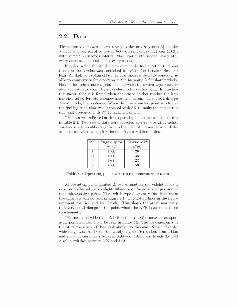
The data was collected at three operating points, which can be seenin table 2.1. Two sets of data were collected at every operating point,one to use when calibrating the models, the estimation data, and theother to use when validating the models, the validation data.
No. Engine speed Engine load[rpm] [Nm]
1 1500 262a 1800 382b 1800 383 2500 50
Table 2.1: Operating points where measurements were taken.
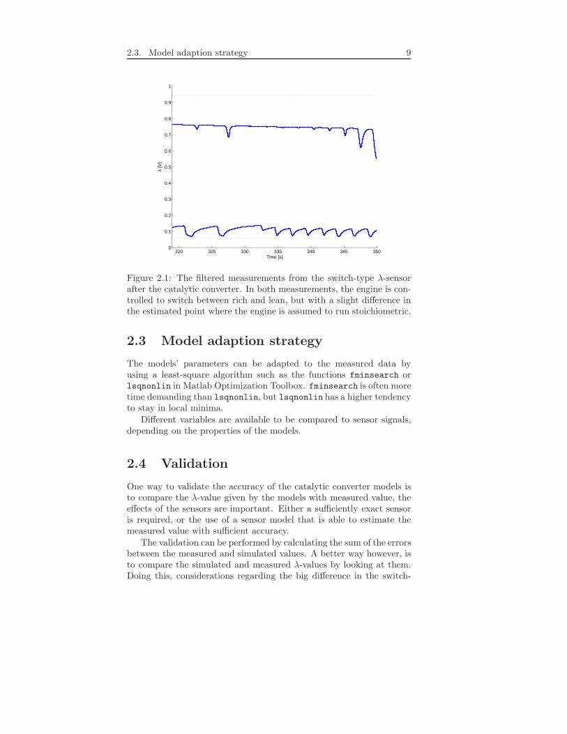
At operating point number 2, two estimation and validation datasets were collected with a slight difference in the estimated position ofthe stoichiometric point. The switch-type λ-sensor values from thesetwo data sets can be seen in figure 2.1. The dotted lines in the figurerepresent the rich and lean levels. This shows the great sensitivityto a very small change in the point where the AFR is assumed to bestoichiometric.
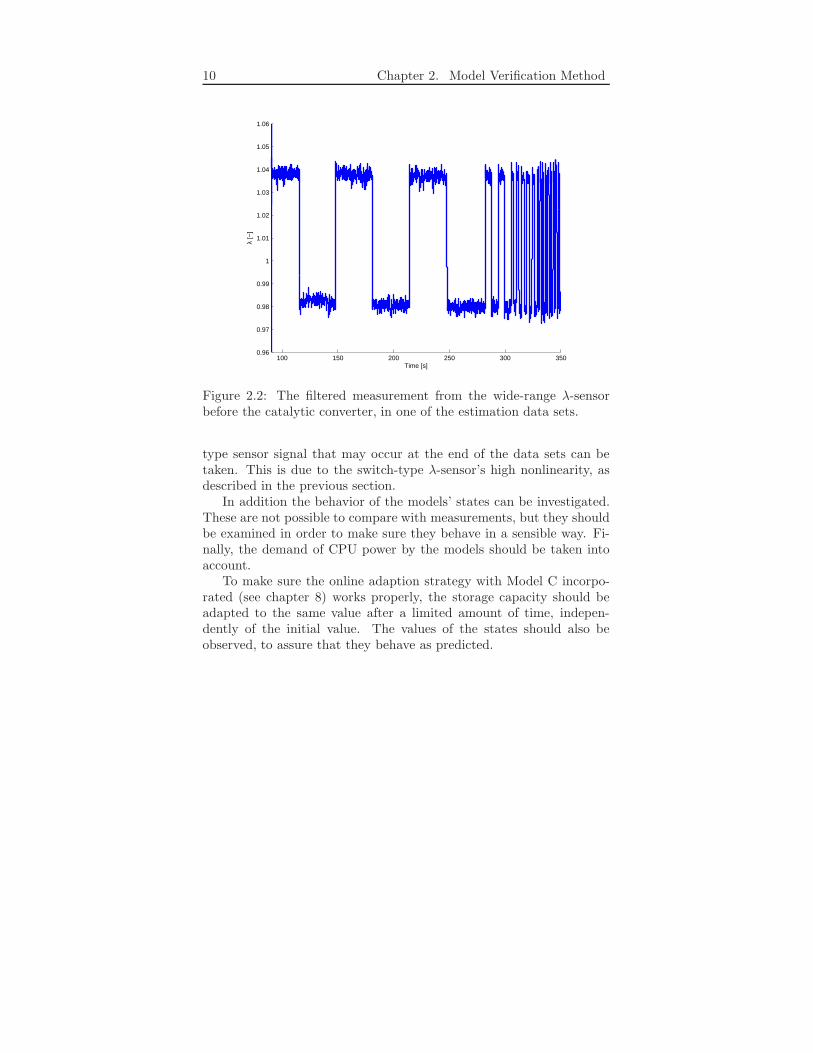
The measured wide-range λ before the catalytic converter at oper-ating point number 3 can be seen in figure 2.2. The measurements inthe other three sets of data look similar to this one. Notice that thewide-range λ-sensor before the catalytic converter suffers from a biasand show measurements between 0.98 and 1.04, even though the realλ-value switches between 0.97 and 1.03.
2.3. Model adaption strategy 9
320 325 330 335 340 345 3500
0.1
0.2
0.3
0.4
0.5
0.6
0.7
0.8
0.9
1
λ [V
]
Time [s]
Figure 2.1: The filtered measurements from the switch-type λ-sensorafter the catalytic converter. In both measurements, the engine is con-trolled to switch between rich and lean, but with a slight difference inthe estimated point where the engine is assumed to run stoichiometric.
2.3 Model adaption strategy
The models’ parameters can be adapted to the measured data byusing a least-square algorithm such as the functions fminsearch orlsqnonlin in Matlab Optimization Toolbox. fminsearch is often moretime demanding than lsqnonlin, but lsqnonlin has a higher tendencyto stay in local minima.
Different variables are available to be compared to sensor signals,depending on the properties of the models.
2.4 Validation
One way to validate the accuracy of the catalytic converter models isto compare the λ-value given by the models with measured value, theeffects of the sensors are important. Either a sufficiently exact sensoris required, or the use of a sensor model that is able to estimate themeasured value with sufficient accuracy.
The validation can be performed by calculating the sum of the errorsbetween the measured and simulated values. A better way however, isto compare the simulated and measured λ-values by looking at them.Doing this, considerations regarding the big difference in the switch-
10 Chapter 2. Model Verification Method
100 150 200 250 300 3500.96
0.97
0.98
0.99
1
1.01
1.02
1.03
1.04
1.05
1.06
λ [−
]
Time [s]
Figure 2.2: The filtered measurement from the wide-range λ-sensorbefore the catalytic converter, in one of the estimation data sets.
type sensor signal that may occur at the end of the data sets can betaken. This is due to the switch-type λ-sensor’s high nonlinearity, asdescribed in the previous section.
In addition the behavior of the models’ states can be investigated.These are not possible to compare with measurements, but they shouldbe examined in order to make sure they behave in a sensible way. Fi-nally, the demand of CPU power by the models should be taken intoaccount.
To make sure the online adaption strategy with Model C incorpo-rated (see chapter 8) works properly, the storage capacity should beadapted to the same value after a limited amount of time, indepen-dently of the initial value. The values of the states should also beobserved, to assure that they behave as predicted.
Chapter 3
Introduction to
Emissions and Catalytic
Converters
Cars are equipped with catalytic converters in order to reduce pollu-tants that have negative consequences on both humans and the envi-ronment. In order to reduce the harmful species the catalytic convertercontains noble metals that promote reactions to take place. These re-actions are necessary for the reduction of the dangerous species in theexhaust gas.
3.1 Combustion Engines and Emissions
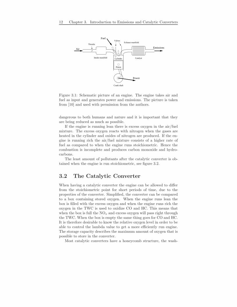
A combustion engine takes air and fuel as input and produces powerand emissions. The fuel is based on hydrocarbons (CαHβ). A schematicpicture of a combustion engine can be found in figure 3.1. When theengine is running stoichiometrically (λ = 1) the fuel and oxygen inthe air are in perfect proportion to each other and theoretically theemissions consists only of carbon dioxide, water vapor and nitrogen,see (3.1).
1
(α+ β4 )λ
CαHβ +O2 +79
21N2
λ=1−−−→
α
(α+ β4 )CO2 +
β/2
(α+ β4 )H2O +
79
21N2 (3.1)
In reality though, small amounts of CO, HC and NOx are producedas well, due to non ideal burning in the cylinders. These species are
11
12 Chapter 3. Introduction to Emissions and Catalytic Converters
⇒
Catalyst
Throttle
Intake manifold
Crank shaft
Piston
Cylinder
Air
Power
Emissions
FuelValves
Exhaust manifold
Figure 3.1: Schematic picture of an engine. The engine takes air andfuel as input and generates power and emissions. The picture is takenfrom [10] and used with permission from the authors.
dangerous to both humans and nature and it is important that theyare being reduced as much as possible.
If the engine is running lean there is excess oxygen in the air/fuelmixture. The excess oxygen reacts with nitrogen when the gases areheated in the cylinder and oxides of nitrogen are produced. If the en-gine is running rich the air/fuel mixture consists of a higher rate offuel as compared to when the engine runs stoichiometric. Hence thecombustion is incomplete and produces carbon monoxide and hydro-carbons.
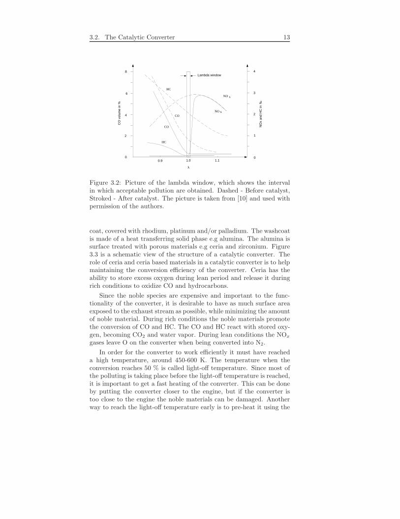
The least amount of pollutants after the catalytic converter is ob-tained when the engine is run stoichiometric, see figure 3.2.
3.2 The Catalytic Converter
When having a catalytic converter the engine can be allowed to differfrom the stoichiometric point for short periods of time, due to theproperties of the converter. Simplified, the converter can be comparedto a box containing stored oxygen. When the engine runs lean thebox is filled with the excess oxygen and when the engine runs rich theoxygen in the TWC is used to oxidize CO and HC. This means thatwhen the box is full the NOx and excess oxygen will pass right throughthe TWC. When the box is empty the same thing goes for CO and HC.It is therefore desirable to know the relative oxygen level in order to beable to control the lambda value to get a more efficiently run engine.The storage capacity describes the maximum amount of oxygen that ispossible to store in the converter.
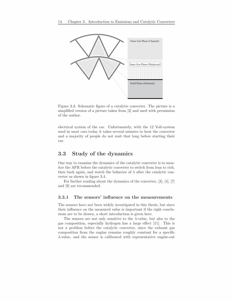
Most catalytic converters have a honeycomb structure, the wash-
3.2. The Catalytic Converter 13
HC
NO
CO
CO
HC
NO
x
x
1.0 1.10.9
4
2
0
6
8
CO
vol
ume
in %
1
2
3
4
0
NO
x an
d H
C in
‰
λ
Lambda window
Figure 3.2: Picture of the lambda window, which shows the intervalin which acceptable pollution are obtained. Dashed - Before catalyst,Stroked - After catalyst. The picture is taken from [10] and used withpermission of the authors.
coat, covered with rhodium, platinum and/or palladium. The washcoatis made of a heat transferring solid phase e.g alumina. The alumina issurface treated with porous materials e.g ceria and zirconium. Figure3.3 is a schematic view of the structure of a catalytic converter. Therole of ceria and ceria based materials in a catalytic converter is to helpmaintaining the conversion efficiency of the converter. Ceria has theability to store excess oxygen during lean period and release it duringrich conditions to oxidize CO and hydrocarbons.
Since the noble species are expensive and important to the func-tionality of the converter, it is desirable to have as much surface areaexposed to the exhaust stream as possible, while minimizing the amountof noble material. During rich conditions the noble materials promotethe conversion of CO and HC. The CO and HC react with stored oxy-gen, becoming CO2 and water vapor. During lean conditions the NOx
gases leave O on the converter when being converted into N2.
In order for the converter to work efficiently it must have reacheda high temperature, around 450-600 K. The temperature when theconversion reaches 50 % is called light-off temperature. Since most ofthe polluting is taking place before the light-off temperature is reached,it is important to get a fast heating of the converter. This can be doneby putting the converter closer to the engine, but if the converter istoo close to the engine the noble materials can be damaged. Anotherway to reach the light-off temperature early is to pre-heat it using the
14 Chapter 3. Introduction to Emissions and Catalytic Converters
Solid Phase (Substrate)
Inner Gas Phase (Washcoat)
Outer Gas Phase (Channel)
Figure 3.3: Schematic figure of a catalytic converter. The picture is asimplified version of a picture taken from [3] and used with permissionof the author.
electrical system of the car. Unfortunately, with the 12 Volt-systemused in most cars today it takes several minutes to heat the converterand a majority of people do not wait that long before starting theircar.
3.3 Study of the dynamics
One way to examine the dynamics of the catalytic converter is to mon-itor the AFR before the catalytic converter to switch from lean to rich,then back again, and watch the behavior of λ after the catalytic con-verter as shown in figure 3.4.
For further reading about the dynamics of the converter, [3], [4], [7]and [9] are recommended.
3.3.1 The sensors’ influence on the measurements
The sensors have not been widely investigated in this thesis, but sincetheir influence on the measured value is important if the right conclu-sions are to be drawn, a short introduction is given here.
The sensors are not only sensitive to the λ-value, but also to thegas composition, especially hydrogen has a large effect [11]. This isnot a problem before the catalytic converter, since the exhaust gascomposition from the engine remains roughly constant for a specificλ-value, and the sensor is calibrated with representative engine-out
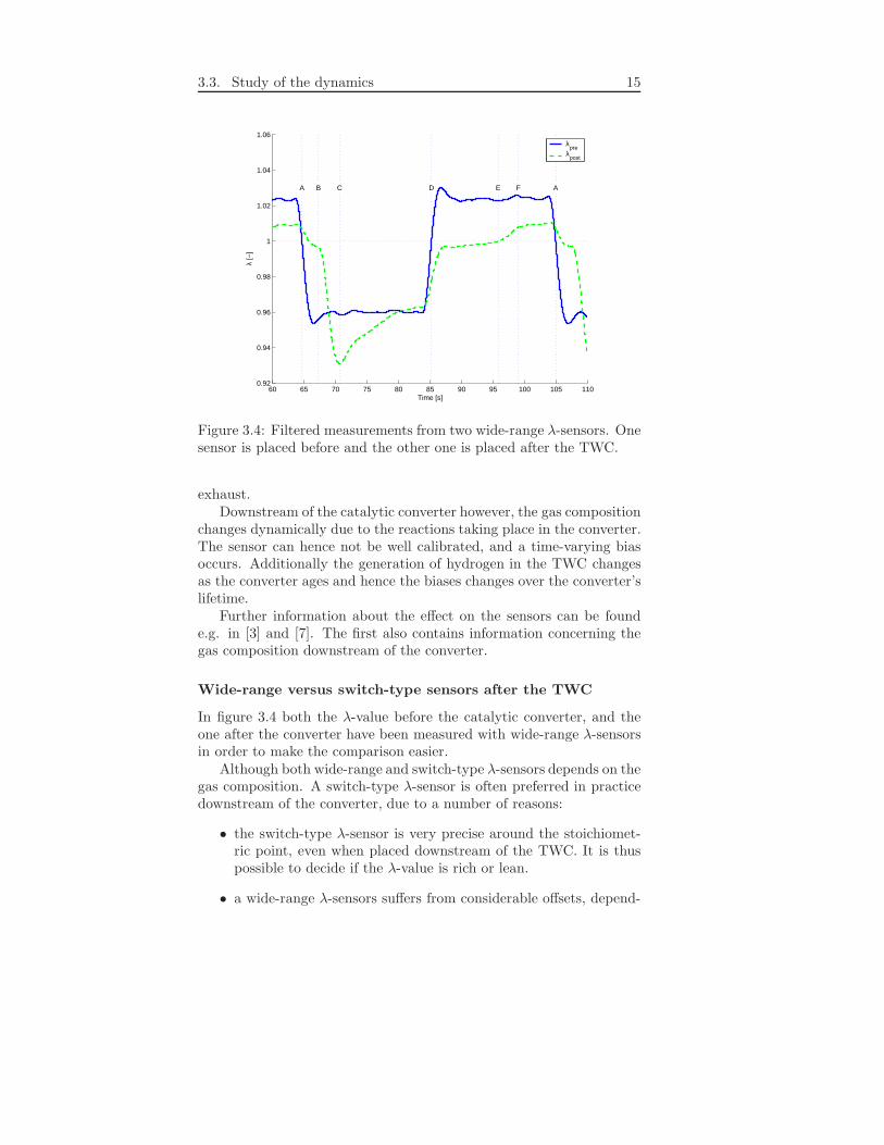
3.3. Study of the dynamics 15
60 65 70 75 80 85 90 95 100 105 1100.92
0.94
0.96
0.98
1
1.02
1.04
1.06
A B C D E F A
λ [−
]
Time [s]
λpre
λpost
Figure 3.4: Filtered measurements from two wide-range λ-sensors. Onesensor is placed before and the other one is placed after the TWC.
exhaust.Downstream of the catalytic converter however, the gas composition
changes dynamically due to the reactions taking place in the converter.The sensor can hence not be well calibrated, and a time-varying biasoccurs. Additionally the generation of hydrogen in the TWC changesas the converter ages and hence the biases changes over the converter’slifetime.
Further information about the effect on the sensors can be founde.g. in [3] and [7]. The first also contains information concerning thegas composition downstream of the converter.
Wide-range versus switch-type sensors after the TWC
In figure 3.4 both the λ-value before the catalytic converter, and theone after the converter have been measured with wide-range λ-sensorsin order to make the comparison easier.
Although both wide-range and switch-type λ-sensors depends on thegas composition. A switch-type λ-sensor is often preferred in practicedownstream of the converter, due to a number of reasons:
• the switch-type λ-sensor is very precise around the stoichiomet-ric point, even when placed downstream of the TWC. It is thuspossible to decide if the λ-value is rich or lean.
• a wide-range λ-sensors suffers from considerable offsets, depend-
16 Chapter 3. Introduction to Emissions and Catalytic Converters
ing on the ageing level of the converter and the sensor
• a switch-type λ-sensor is cheaper than a wide-range. Additionallya switch-type λ-sensor is already in use for diagnostic purposesin modern cars, therefore no extra sensor is needed.
3.3.2 Study of the measurements
To make the references shorter in this section all capital letters in brack-ets should be interpreted as references to the corresponding time stampsin figure 3.4.
Both the λ-values before and after the catalytic converter, have beenmeasured with wide-range λ-sensors. It should be noted however, thatthe characteristics of the sensors are different, and tests have shown thatthere are offset and gain differences between them even when placed onthe same side of the converter.
Before the point where the wide-range λ-sensor before the converter,λpre, switches from lean to rich (A) the engine has been running leanfor quite a while and thus the amount of stored oxygen in the catalyticconverter is high and the degree of catalyst deactivation is low. Thedifferences in λpre and the wide-range λ-sensor after the converter,λpost, should not be paid too much attention because of the differencebetween the sensors and the influence of the change in gas composition.
Directly after λpre switches from lean to rich (between A and B)λpost stays close to the stoichiometric level even though λpre is rich.This is because of the large amount of excess oxygen in the catalyticconverter that compensates for the lack of oxygen in the incoming gas.λpost does not start to fall until the converter is out of excess oxygen(B). Then λpost drops to its richest value (C).
During the interval between (B) and (C) the oxygen storage leveldecreases even more to compensate for the lack of oxygen in the in-coming gas. At the same time, the degree of catalyst deactivation isslightly increased due to the rich incoming gas that cannot be oxidizeddue to the lack of excess oxygen. Hence, the engine is running rich andthere is a high amount of vacant sites on the converter’s surface, whichpromotes the hydrogen generating reactions listed in appendix A. Theincreasing amount of hydrogen makes the λpost-sensor show a richervalue than the true one. This explains the big difference between λpostand λpre at (C).
In the interval between (C) and (D) where both λpre and λpostshow rich values, the degree of catalyst deactivation is continuouslyincreased since there are more species that needs to be oxidized thanavailable oxygen. Hence, the number of vacant sites is decreased, andthe hydrogen generation is inhibited. This affects the λpost-sensor,which shows an increasingly leaner value.
3.3. Study of the dynamics 17
When λpre switches back to lean (D), λpost stays close to the sto-ichiometric level in the same way as when λpre switched to rich. Atfirst, the excess oxygen in the incoming gas works to oxidize the speciesthat have been gathered in the catalytic converter during the rich pe-riod and caused the catalyst deactivation. Then the excess oxygen inthe incoming gas is adsorbed in the converter and increases the level ofstored oxygen again.
λpost starts to increase when the catalytic converter is close to fullwith oxygen (E) and reaches it’s leanest level (F) then stays at the leanlevel until λpre switches from lean to rich (A) and everything startsover again.
The reason why the interval between (D) and (E) is much furtherin time than the interval between (A) and (B) is probably mostly dueto biases in the system. Even though the response time when the λis switched between rich and lean might differ from the response timewhen it switches from lean to rich.
Both the λ-value measured by the control system, as well as theλ-sensors may suffer from biases. The control system is operated toswitch the λ-value between 0.97 and 1.03 but as can be seen in figure3.4 the measured λpre is lower than that. Hence, it is possible thatthe engine is running very rich when running rich, but only slightlylean when running lean, which would explain the difference in time toincrease/decrease the catalyst deactivation and fill/empty the converterof stored oxygen.

18
Chapter 4
Model A - A Storage
Dominated Model with
Reversible Catalyst
Deactivation
This chapter describes a model presented by James C. Peyton Jones in[6] and [8]. It is empirical and it is assumed that the dynamics of thecatalytic converter are dominated by oxygen storage in the converterand reversible catalyst deactivation. These are not assumed to changeover the catalytic converter’s spatially distributed nature. Hence, thereare two state space variables to describe these two phenomena. Thisis based on the observation in [6] that all gas components respond toinput changes over a similar time-scale. Which shows that the processis dominated by the relatively slow dynamics of gas storage and re-lease, and that the other kinetics occur over a much shorter, and lesssignificant, time-scale.
4.1 Model
The model has one input, the wide-range λ-value before the catalyticconverter, and one output, the wide-range λ-value after the converter.
Note that the AFR in this model is expressed in terms of the dif-ference from stoichiometric, ∆λ = λ− 1, instead of the more commonλ. This makes it possible to model the states of the catalytic converterwith a single integrator.
19
20 Chapter 4. Model A - A Storage Dominated Model with ...
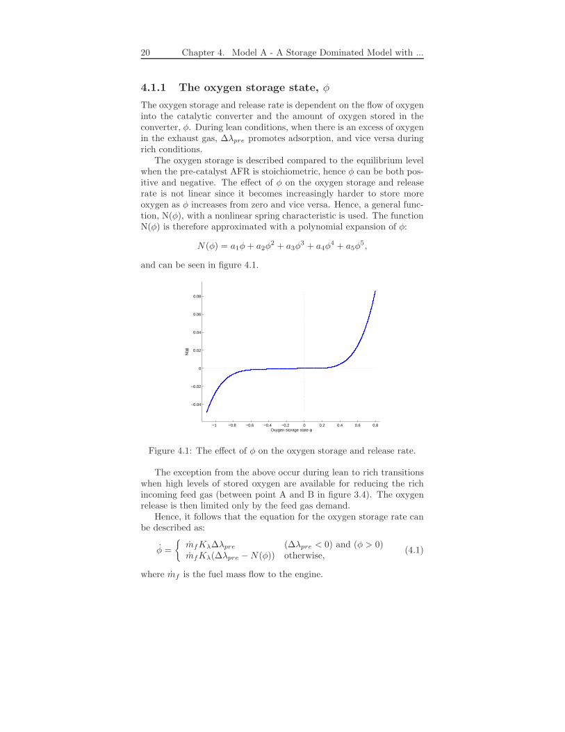
4.1.1 The oxygen storage state, φ
The oxygen storage and release rate is dependent on the flow of oxygeninto the catalytic converter and the amount of oxygen stored in theconverter, φ. During lean conditions, when there is an excess of oxygenin the exhaust gas, ∆λpre promotes adsorption, and vice versa duringrich conditions.
The oxygen storage is described compared to the equilibrium levelwhen the pre-catalyst AFR is stoichiometric, hence φ can be both pos-itive and negative. The effect of φ on the oxygen storage and releaserate is not linear since it becomes increasingly harder to store moreoxygen as φ increases from zero and vice versa. Hence, a general func-tion, N(φ), with a nonlinear spring characteristic is used. The functionN(φ) is therefore approximated with a polynomial expansion of φ:
N(φ) = a1φ+ a2φ2 + a3φ
3 + a4φ4 + a5φ
5,
and can be seen in figure 4.1.
−1 −0.8 −0.6 −0.4 −0.2 0 0.2 0.4 0.6 0.8
−0.04
−0.02
0
0.02
0.04
0.06
0.08
Oxygen storage state φ
N(φ
)
Figure 4.1: The effect of φ on the oxygen storage and release rate.
The exception from the above occur during lean to rich transitionswhen high levels of stored oxygen are available for reducing the richincoming feed gas (between point A and B in figure 3.4). The oxygenrelease is then limited only by the feed gas demand.
Hence, it follows that the equation for the oxygen storage rate canbe described as:
φ =
{
mfKλ∆λpre (∆λpre < 0) and (φ > 0)mfKλ(∆λpre −N(φ)) otherwise,
(4.1)
where mf is the fuel mass flow to the engine.
4.2. Convert to switch type λ-values 21
4.1.2 The reversible catalyst deactivation, ψ
The deactivated fraction of the catalytic converter surface increaseswhen there is a deficiency of oxygen both before the converter and af-ter, i.e. when there is a deficiency of oxygen in the incoming feed gasand not enough oxygen stored in the converter to compensate for this(between point B and D in figure 3.4). The rate at which the deactiva-tion increases is proportional to the mass flow into the converter, thelack of oxygen after the catalytic converter, −∆Λpost, and the fractionof the surface already occupied by deactivation agents, ψ. The pres-ence of excess oxygen in the feed gas, ∆λpre > 0, on the other handdecreases the deactivation at a rate proportional to the supply of oxy-gen in the feed gas, until there are no more deactivation agents left onthe surface, ψ = 0, (just after point D in figure 3.4).
The deactivated fraction of the catalytic converter surface, ψ, canhence be described as follows:
ψ =
mfKd(∆Λpost − ψ) (∆λpre < 0) and (∆Λpost < 0)−mfKr∆λpre (∆λpre > 0) and (ψ > 0)0 otherwise.
(4.2)
Note that ∆Λpost is the post-catalyst AFR deviation from stoichio-metric before the effect of the catalyst deactivation has been taken intoaccount, and thus not equal to ∆λpost, which is the ∆λ-value after thecatalytic converter.
4.1.3 Estimated ∆λ value after the catalytic con-
verter
The ∆λ value after the catalytic converter depends on the ∆λ valuebefore the converter, the rate at which oxygen is released compared tothe fuel mass flow, and the deactivated fraction of the converter.
∆λpost = ∆λpre −1
mfKλφ+Kψψ
=
{
Kψψ (∆λpre < 0) and (φ > 0)N(φ) +Kψψ otherwise
(4.3)
The received output from this model is thus a λ-value that can becompared to the output from a wide-range λ-sensor.
4.2 Convert to switch type λ-values
To be able to use the wide-range λ-value obtained from the modelfor control purposes, a reliable wide-range λ-sensor after the catalyticconverter is needed. In the articles [6] and [8], the measured values
22 Chapter 4. Model A - A Storage Dominated Model with ...
agree well with the values achieved with the model. The oxygen storagestate describes the dynamics of the oxygen filling and depleting, andthe distortion of the λ-sensor is taken into account by the reversiblecatalyst deactivation state. The wide-range λ-sensor used after theconverter in this thesis however, suffers from biases and attempts toadapt the model to measured data failed.
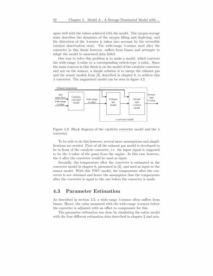
One way to solve this problem is to make a model, which convertsthe wide-range λ-value to a corresponding switch-type λ-value. Sincethe main concern in this thesis is on the model of the catalytic converterand not on the sensors, a simple solution is to merge the exhaust gasand the sensor models from [3], described in chapter 6, to achieve thisλ converter. The augmented model can be seen in figure 4.2.
fuel
mass flowExhaust
gas
model
Catalytic
converter
model
Switch
type
λ-sensor
model
Exhaust temperature
Switch-
type
λ-value
λ converter model
wide-range
λ-value
wide-range
λ-value
Figure 4.2: Block diagram of the catalytic converter model and the λconverter.
To be able to do this however, several more assumptions and simpli-fications are needed. First of all the exhaust gas model is developed tobe in front of the catalytic converter, i.e. the input signal is supposedto be the λ-value of the gases from the engine. In this case however,the λ after the converter would be used as input.
Secondly, the temperature after the converter is estimated in theconverter model in chapter 6, presented in [3], and used as input to thesensor model. With this TWC model, the temperature after the con-verter is not obtained and hence the assumption that the temperatureafter the converter is equal to the one before the converter is made.
4.3 Parameter Estimation
As described in section 3.3, a wide-range λ-sensor often suffers frombiases. Hence, the value measured with the wide-range λ-sensor beforethe converter is adjusted with an offset to compensate for this.
The parameter estimation was done by simulating the entire modelwith the four different estimation data described in chapter 2 and min-
4.3. Parameter Estimation 23
imizing the sum of the square error. This can be done according to thescheme below:
• Use the function fminsearch in Matlab Optimization Toolbox inorder to estimate the parameters in the catalytic converter model.The first time this is done, the start values of the parametersin the exhaust gas and sensor models can be set to the valuesobtained in chapter 6.
• Use the function fminsearch in order to estimate the parametersin the exhaust gas model.
• Once again, use the function fminsearch and estimate the pa-rameters in the sensor model.
• Depending on the accuracy of the start values, the previous threesteps might have to be repeated. When reasonable values havebeen obtained, the function lsqnonlin in Matlab OptimizationToolbox can be used to estimate all of the parameters, to finallytune them.
The resulting parameter values can be found in appendix B.
Since the model is highly nonlinear it is hard to find the parametersthat are optimal in a global sense, and a large number of optimiza-tion steps might have to be made to obtain good estimations of theparameters.
4.3.1 Catalytic Converter Parameters
The parameters that need to be estimated in this model of the catalyticconverter are:
Kλ , a constant of proportionality, which affects the rate at which theoxygen storage state changes.
Kd , the deactivation constant of proportionality, i.e. it affects the rateat which the deactivation increases.
Kr , the reactivation constant of proportionality, i.e. it affects the rateat which the deactivation decreases.
Kψ , a constant of proportionality, which represents the effect the re-versible catalyst deactivation has on the λpost-value.
a1...a5 , the coefficients in the polynomial describing N(φ).
24 Chapter 4. Model A - A Storage Dominated Model with ...
4.3.2 Exhaust Gas and Sensor Parameters
The parameters in the exhaust gas and sensor models are estimated inorder to adjust the models to the new conditions, i.e. that the exhaustgas model is placed behind the model of the catalytic converter insteadof in front, and the temperature used as input to the sensor model isthe one of the exhaust gases instead of the temperature of the gasesafter the converter.
The parameters to be estimated in the exhaust gas model are:
aηcomb, bηcomb
, and φH2/CO,
and the ones in the sensor model are:
Aλst, Bλst, Cλst, Dλst, EA,λst, EE,λst, and Fλst.
4.3.3 Parameters adjusted to the age of the con-
verter
The catalytic converter’s behavior changes as a result of the ageing ofthe converter. Hence, some parameter values are adjusted over time toaccount for this. According to [12] it is the converter’s storage capacitythat is affected. Thus, the parameters that need to be adjusted are theones, which affect mainly the increase of the oxygen storage rate andthe increase of the catalyst deactivation.
The oxygen storage rate depend on the parameter Kλ and the co-efficients in the polynomial N(φ), i.e. a1 to a5. Since Kλ is the onlyparameter that affects the decrease during lean to rich transitions whenhigh levels of stored oxygen are available, and this rate should be signif-icantly the same over time, Kλ is not adjusted. Hence, the parametersthat do need to be adjusted are the coefficients a1 to a5.
The catalyst deactivation rate depend on the parameter Kd whenit is increasing and Kr when it is decreasing. Therefore, it is the pa-rameter Kd that should be adjusted.
The only remaining parameter in the converter model not consid-ered is Kψ. This represents the effect the reversible catalyst deactiva-tion has on the λpost-value and should not be significantly dependenton the converters age.
To sum up, the parameter Kd and the coefficients a1 to a5 shouldbe adjusted as the converter is ageing.
4.4 Discussion
The model of the catalytic converter and the merged λ converter areevaluated in order to see if they together make a good estimation of the
4.4. Discussion 25
switch-type λ-value after the converter, and if the states act the waythey are expected to.
4.4.1 The extension to switch-type λ-values
As mentioned earlier two large simplifications were made to be ableto merge the exhaust gas model and the sensor model in chapter 6,presented in [3], into a λ converter.
The first one was that the exhaust gas model could be used after thecatalytic converter, instead of before the converter. The composition ofthe gases for a specific λ-value before the converter is roughly constant,as described in section 3.3. This knowledge is used when the concen-trations are calculated in the exhaust gas model. The gas compositiondownstream of the converter however, changes dynamically (also thisis described in section 3.3). This model should thus not be expected toproduce the correct concentrations at e.g. different operating points.
The second simplification was to use the exhaust gas temperaturebefore the converter instead of the one after the TWC as input tothe exhaust gas and the sensor model. In reality, the behavior of theexhaust gas temperature before and after the converter is very different.When the engine is running rich, the exhaust gas temperature is low.This leads to a high amount of unburned fuel that instead reaches theconverter and makes the temperature rise in the gases that leaves theTWC. Hence, in this case, low exhaust gas temperatures lead to highertemperatures of the gases after the converter.
In order to make the exhaust gas and sensor models as accurate aspossible under these new conditions, the parameters in the models wereestimated in this chapter as well. However, it should be noted that theresulting λ converter not is expected to be very reliable. A benefit fromusing it though, is that a switch-type λ-sensor can be used downstreamof the converter, instead of a wide-range. As described in section 3.3,a switch-type sensor is often preferred.
Parameter values in the exhaust gas and sensor models
The adjustments made in the parameters can be seen when comparingthe values of the parameters obtained in this chapter, which can befound in appendix B, with the values estimated in 6, found in appendixC.
In the exhaust gas model, the coefficients relating to the temper-ature, aηcomb
and bηcomb, has changed the sign. Additionally a big
increase in φH2/CO can be seen, which suggests that there are a lotmore hydrogen as compared to CO in the gas after the converter thanbefore, as expected.
26 Chapter 4. Model A - A Storage Dominated Model with ...
In the sensor model’s parameters the major differences can be foundin the parameters Bλst, Cλst, Dλst and EE,λst. The first three is directlyconnected to the concentrations, i.e. the output from the exhaust gasmodel, and the fourth to the temperature.
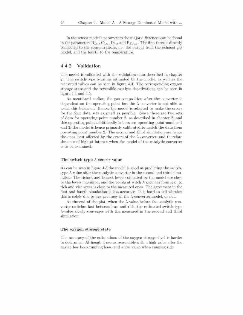
4.4.2 Validation
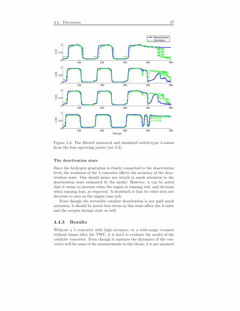
The model is validated with the validation data described in chapter2. The switch-type λ-values estimated by the model, as well as themeasured values can be seen in figure 4.3. The corresponding oxygenstorage state and the reversible catalyst deactivations can be seen infigure 4.4 and 4.5.
As mentioned earlier, the gas composition after the converter isdependent on the operating point but the λ converter is not able tocatch this behavior. Hence, the model is adapted to make the errorsfor the four data sets as small as possible. Since there are two setsof data for operating point number 2, as described in chapter 2, andthis operating point additionally is between operating point number 1and 3, the model is hence primarily calibrated to match the data fromoperating point number 2. The second and third simulation are hencethe ones least affected by the errors of the λ converter, and thereforethe ones of highest interest when the model of the catalytic converteris to be examined.
The switch-type λ-sensor value
As can be seen in figure 4.3 the model is good at predicting the switch-type λ-value after the catalytic converter in the second and third simu-lation. The richest and leanest levels estimated by the model are closeto the levels measured, and the points at witch λ switches from lean torich and vice versa is close to the measured ones. The agreement in thefirst and fourth simulation is less accurate. It is hard to tell whetherthis is solely due to less accuracy in the λ-converter model, or not.
At the end of the plot, when the λ-value before the catalytic con-verter switches fast between lean and rich, the estimated switch-typeλ-value slowly converges with the measured in the second and thirdsimulation.
The oxygen storage state
The accuracy of the estimations of the oxygen storage level is harderto determine. Although it seems reasonable with a high value after theengine has been running lean, and a low value when running rich.
4.4. Discussion 27
150 200 250 300 3500
0.5
1
λ [V
]
MeasurementSimulation
150 200 250 300 3500
0.5
1
λ [V
]
150 200 250 300 3500
0.5
1
λ [V
]
150 200 250 300 3500
0.5
1
λ [V
]
Time [s]
Figure 4.3: The filtered measured and simulated switch-type λ-valuesfrom the four operating points (see 2.2).
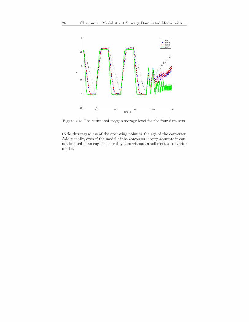
The deactivation state
Since the hydrogen generation is closely connected to the deactivationlevel, the weakness of the λ converter affects the accuracy of the deac-tivation state. One should hence not attach to much attention to thedeactivation state estimated by the model. However, it can be notedthat it seems to increase when the engine is running rich, and decreasewhen running lean, as expected. A drawback is that its value does notdecrease to zero as the engine runs rich.
Even though the reversible catalyst deactivation is not paid muchattention, it should be noted that errors in this state affect the λ-valueand the oxygen storage state as well.
4.4.3 Results
Without a λ converter with high accuracy, or a wide-range λ-sensorwithout biases after the TWC, it is hard to evaluate the model of thecatalytic converter. Even though it captures the dynamics of the con-verter well for some of the measurements in this thesis, it is not assumed
28 Chapter 4. Model A - A Storage Dominated Model with ...
150 200 250 300 350−1.5
−1
−0.5
0
0.5
1
Time [s]
φ
op1op2aop2bop3
Figure 4.4: The estimated oxygen storage level for the four data sets.
to do this regardless of the operating point or the age of the converter.Additionally, even if the model of the converter is very accurate it can-not be used in an engine control system without a sufficient λ convertermodel.
4.4. Discussion 29
150 200 250 300 350−2
0
2
4
6
8
10x 10
−4
Time [s]
ψ
op1op2aop2bop3
Figure 4.5: The estimated reversible deactivation fraction for the fourdata sets.

30

Chapter 5
Model B - A Model
Consisting of One
Nonlinear Integrator
This model is presented by Mario Balenovic in [4]. The model is basi-cally a nonlinear integrator with one state representing oxygen cover-age, one parameter which gives an indication on the converters’ storagecapacity and a function that represents the relative conversion. Themodel has one input and one output, the wide-range λ-sensor signalsbefore and after the catalytic converter, respectively.
5.1 Model
The model is developed in order to control the engine based on the stateof the catalytic converter. In this case the desired controlled variableis the degree of ceria coverage by oxygen containing species (relativeoxygen coverage of ceria, ROC).
5.1.1 Model developement
Model assumptions:
• The dynamic behavior of the catalytic converter is only due tothe oxygen storage and release capabilities of ceria.
• Reactions taking place on the noble metal surface are assumed tobe instantaneous.
• The oxygen storage filling can be represented by a single variable.
31
32 Chapter 5. Model B - A Model Consisting of One Nonlinear...
• Both the lambda sensors (before and after the catalytic converter)are ideal
• CO is not taken into account when calculating the relative oxygencoverage of ceria.
It is also assumed that there are only CO and O2 in the exhausts andthat the converters’ length is almost zero. These assumptions make itpossible to model only one point in the converter. The species can reactin the converter either by surface reactions or by oxidation or reductionon the ceria. The outgoing concentration of CO is the incoming con-centration of CO minus the CO that reacts on the surface and the COthat reacts with ceria. The same goes for O2. The surface reactionsare assumed to be immediate. This means that the incoming CO or O2
and the CO or O2 that is left after the reaction with the surface canbe called the excess of the species. Then the outlet concentrations forrich inlet feed can be written as following:
cCOout = cCOex − rCO
cO2out = 0(5.1)
and for lean inlet feed:
cCOout = 0
cO2out = cO2ex − rO2
. (5.2)
The subscript ex denotes the excess of the species after a surface reac-tion has been completed and r is the reaction rate on the ceria.
During lean conditions the disappearance rate of excess O2 is pro-portional to the oxygen storage filling:
rO2∼dξ
dt=
1
LkfillcO2
(1 − ξ). (5.3)
Correspondingly the disappearance rate of excess CO during rich con-ditions is proportional to the oxygen storage emptying:
rCO ∼ −dξ
dt= −
1
LkempcO2
θCOξ, (5.4)
where ξ is the local fraction of oxygen storage. These equations arebased on equations from a more advanced model, also presented in [4].
The λ value can be expressed in terms of oxidants (O), reactants(R) and products (P):
λ =O + P
R+ P, P ≫ O,P ≫ R. (5.5)
5.1. Model 33
It will be assumed that all oxidants can oxidize ceria and all reactantscan reduce ceria. Only the excess of reactants or oxidants will be neededfor the model input, hence the following holds:
λlean ≈OexP
+ 1
λrich ≈ 1 −RexP
. (5.6)
In order to get the λrich equation a first order Taylor series has beenused. This holds as long as the input does not become very rich. Sinceonly the excess of reactants or oxidants will be needed for model inputthe lambda excess, λ − 1, will be used. The lambda excess will bedenoted ∆λ. Taking into account (5.1) and (5.2) the final model (forone point of the converter) that holds in both lean and rich regionsbecomes:
∆λout = ∆λin − kddξ
dt. (5.7)
Replacing the local variable ξ with ζ representing the relative oxygencoverage of ceria for the whole reactor, this model is valid also for thewhole converter. Since the complete reactor is modeled as a series ofalmost zero-length reactors the expressions (5.3) and (5.4) has to bemodified. Since they become nonlinear when more than one reactor isconnected in series an alternative approach has to be taken. The globalreaction rate can therefore be expressed as:
dζ
dt= kgr∆λinf(ζ). (5.8)
kgr is a scaling factor and the function f(ζ) is a nonlinear functiondepending on the inlet feed. f(ζ) is in fact two functions, fL for leaninput and fR for rich input. If (5.7) and (5.8) are put together theexpression for ∆λ becomes:
∆λout = ∆λin(1 − kdkgrf(ζ)) (5.9)
.Under the assumption that the outlet lambda cannot have the op-
posite sign of the inlet lambda, (1 − kdkgrf(ζ)) cannot be below 0 orexceed l. This means that kdkgrf(ζ) also is bounded in the same inter-val. Since the function f has to be estimated the two scaling factorscan be included in f . It will also be assumed that kgr = 1
kd. Thus, the
model becomes:
dζ
dt=
1
kd∆λinf(ζ) (5.10)
∆λout = ∆λin − kddζ
dt(5.11)
= ∆λin(1 − f(ζ)). (5.12)
34 Chapter 5. Model B - A Model Consisting of One Nonlinear...
5.1.2 The complete model
The assumption that the inlet and outlet lambda value cannot haveopposite signs is not always true. During a rich-to-lean step the outletstays rich for a short period of time even though the inlet is lean, see[4]. This can also be seen after point D in figure 3.4. This is due to COand HC desorption from the ceria surface and the noble metal surface.The model (5.10) cannot describe this, thus some modification shouldbe made. One way of solving this is to add an additional function toaccount for the desorption effect. The final model becomes:
dζ
dt=
1
kd(∆λinf(ζ) + g(ζ) (5.13)
∆λout = ∆λin − kddζ
dt(5.14)
= ∆λin(1 − f(ζ)) + g(ζ). (5.15)
The strictly positive function g(ζ) is only activated when the inlet isstoichiometric or lean and thus it is possible to model rich output withlean inputs.
5.1.3 Model parameters and functions
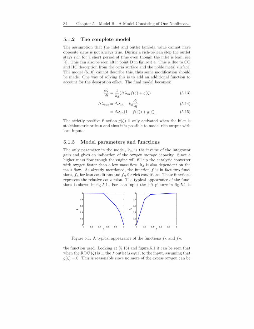
The only parameter in the model, kd, is the inverse of the integratorgain and gives an indication of the oxygen storage capacity. Since ahigher mass flow trough the engine will fill up the catalytic converterwith oxygen faster than a low mass flow, kd is also dependent on themass flow. As already mentioned, the function f is in fact two func-tions, fL for lean conditions and fR for rich conditions. These functionsrepresent the relative conversion. The typical appearance of the func-tions is shown in fig 5.1. For lean input the left picture in fig 5.1 is
0 0.2 0.4 0.6 0.8 10
0.2
0.4
0.6
0.8
1
ζ
f L
0 0.2 0.4 0.6 0.8 10
0.2
0.4
0.6
0.8
1
ζ
f R
Figure 5.1: A typical appearance of the functions fL and fR.
the function used. Looking at (5.15) and figure 5.1 it can be seen thatwhen the ROC (ζ) is 1, the λ outlet is equal to the input, assuming thatg(ζ) = 0. This is reasonable since no more of the excess oxygen can be
5.2. Parameter estimation 35
stored when ζ = 1. The less oxygen stored in the catalytic converter,the closer to 1 fL gets, which means that ∆λout approaches zero, i.e.λ ≈ 1. For rich input it is the other way around. When there is a lot ofstored oxygen almost all of the reducing species in the converter reactswith the stored oxygen and ∆λout is close to zero. When the converteris empty of stored oxygen all the exhaust coming in to the converteralso comes out. Both fL and fR is dependent on the mass flow.
The function g(ζ) has been added to the model in order to be ableto model rich output with lean input. The function is activated onlywhen the input is stoichiometric or lean and is also dependent on themass flow.
Since both parameter and functions are dependent on the mass flow,Balenovic made additional changes in the model in order to make themodel better in a wider operating range. These changes will not bepresented here but can be viewed in [4].
Both parameter and functions are dependent on the mass flow.However, in [4] additional changes in the model is presented, whichmakes the model better in a wider operating range. These changes willnot be presented here.
5.2 Parameter estimation
It is desirable to have an easy parameter estimation algorithm whichcan be used online, since the behavior of the catalytic converter changesover time. The parameter estimation algorithm presented in [4] requiresvery short testing time. The parameters and functions that need to beestimated are kd, f(ζ) and g(ζ). kd is very straight-forward to get.From (5.14) it follows:
kddζ = (∆λin − ∆λout)dt. (5.16)
If a test begins after the engine has run rich for a while and the oxygenstorage is ζ = 0 and ends after Tss seconds with a completely filledoxygen storage the following holds:
kd =
∫ Tss
0 (∆λin − ∆λout)dt∫ 1
0dζ
=
∫ Tss
0
(∆λin − ∆λout)dt
. (5.17)
The same approach can be used when the catalytic converter is initiallyfilled and empty at the end of the test. (5.17) can be approximatedwith the following sum:
kd =
N∑
k=1
(∆λin(k) − ∆λout(k))Ts, (5.18)
36 Chapter 5. Model B - A Model Consisting of One Nonlinear...
where N is the total number of samples and Ts is the sampling time.The same data and the same equation can be used to get ζ(t) which
can be used to estimate the function f(ζ) (g(ζ) is neglected here). From(5.15) it follows:
f(ζ) = 1 −∆λout∆λin
. (5.19)
When calculating (5.19) for all samples, F(k) is obtained. Instead of
using a map with F(k) and ζ(k) a simpler function f(ζ) is calculated
with a least squares algorithm. f(ζ) is approximated by a piecewiselinear function. This function can be written as a linear combinationof triangular basis functions:
f(ζ) =
∑ni=1 bi(ζ)fi
∑ni=1 bi()ζ
, (5.20)
where the triangular basis functions are:
bi(ζ) =
0, if ζ < ζi−1, i ≥ 2ζ−ζi−1
ζi−ζi−1 , if ζi−1 ≤ ζ < ζi, i ≥ 2
1 − ζ−ζi
ζi+1−ζi, if ζi ≤ ζ < ζi+1, i ≤ n− 1
0, if ζ ≥ ζi+1, i ≤ n− 1.
(5.21)
Good results have been obtained in [4] when predefining the basis func-tions. With fixed basis functions equation (5.20) has an analyticalsolution. The parameters f1,2..n are tuning parameters to the n ba-sis functions. A piecewise linear function with five points should beenough. An example on how to solve the least square problem can befound in [4].
The function g(ζ) can be obtained in a similar manner. The dataused to estimate the function is taken during a rich to lean step. Sincethe function only will be used when inlet and outlet lambda have dif-ferent signs and when ∆λin ≥ 0, the data set is calculated by:
G(k) =
{
∆λout, if ∆λout < 00, if ∆λout ≥ 0
(5.22)
F (k) =
{
1, if ∆λout < 0
1 − ∆λout
∆λin, if ∆λout ≥ 0.
(5.23)
The function g(ζ) does not have to be as accurate as f , so a piecewiselinear function with two or three point should be sufficient. g(ζ) can
be calculated in the same manner as f(ζ).
5.3 Validation
During the parameter estimation, the accuracy of the lambda sensorsignals is crucial. Neither the pre nor the post catalytic converter sensor

5.3. Validation 37
can have any biases. No such lambda sensor signals have been availableand therefore the model has not been tested.
The reason why this model is included in this thesis, is that withaccurate λ-sensors, the model should give satisfying result. The modelis also very simple with only one state and it needs no parameter op-timization, only calculations of the parameter and states. Hence, themodel should be easy to fit into an engine control system and needlittle CPU power.

38
Chapter 6
Model C - A Simplified
Physical Exhaust Gas
Aftertreatment Model
This model has been developed by Theophil Sebastian Auckenthalerand is presented in [3]. The model is a physical model of the exhaustgas aftertreatment system, which includes a reversible wide-range λ-sensor model before the converter, a switch-type λ-sensor model afterthe converter, and of course a TWC model.
The model is based on reaction kinetics of a small number of key gascomponents and reactions together with the dynamics of gas storage onthe converter surface. The spatially distributed nature of the converteris approximated by a lumped parameter model. The ageing of theTWC is represented by the parameter describing the storage capacity,hence the storage capacity is the only parameter that is assumed tochange over time.
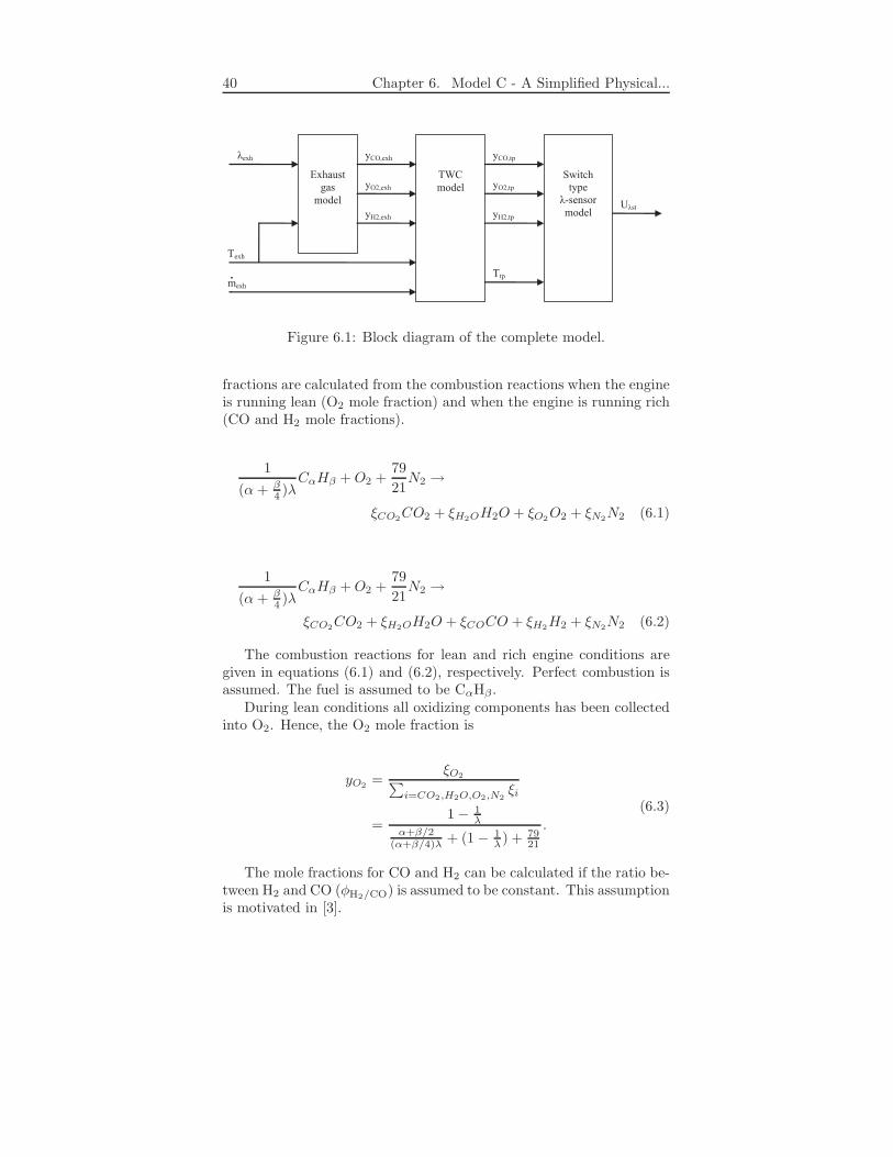
6.1 Model
The model consists of three modules, see fig 6.1.The input to the model is the wide-range lambda sensor signal up-
stream of the TWC, the exhaust mass flow and temperature, and theoutput is the switch-type lambda sensor signal.
6.1.1 Exhaust gas model
The main purpose of the exhaust gas model is to convert the wide-rangelambda sensor value into mole fractions of O2, CO and H2. These mole
39
40 Chapter 6. Model C - A Simplified Physical...
Exhaust
gas
model
TWC
model
Switch
type
λ-sensor
model
λexh
Texh
mexh
yCO,exh
yO2,exh
yH2,exh
yCO,tp
yO2,tp
yH2,tp
Ttp
Uλst
.
Figure 6.1: Block diagram of the complete model.
fractions are calculated from the combustion reactions when the engineis running lean (O2 mole fraction) and when the engine is running rich(CO and H2 mole fractions).
1
(α + β4 )λ
CαHβ +O2 +79
21N2 →
ξCO2CO2 + ξH2OH2O + ξO2
O2 + ξN2N2 (6.1)
1
(α + β4 )λ
CαHβ +O2 +79
21N2 →
ξCO2CO2 + ξH2OH2O + ξCOCO + ξH2
H2 + ξN2N2 (6.2)
The combustion reactions for lean and rich engine conditions aregiven in equations (6.1) and (6.2), respectively. Perfect combustion isassumed. The fuel is assumed to be CαHβ .
During lean conditions all oxidizing components has been collectedinto O2. Hence, the O2 mole fraction is
yO2=
ξO2∑
i=CO2,H2O,O2,N2ξi
=1 − 1
λα+β/2
(α+β/4)λ + (1 − 1λ) + 79
21
.
(6.3)
The mole fractions for CO and H2 can be calculated if the ratio be-tween H2 and CO (φH2/CO) is assumed to be constant. This assumptionis motivated in [3].
6.1. Model 41
yCO =
21+φH2/CO
( 1λ − 1)
α+β/2(α+β/4)λ + 79
21
yH2=
2φH2/CO
1+φH2/CO( 1λ − 1)
α+β/2(α+β/4)λ + 79
21
.
(6.4)
Since species have been lumped together it is important to remem-ber that the mole fractions contain fractions of other species as well.It has been found that it is critical that the final mole fractions areconsistent in terms of the air/fuel ratio λ, but it is not so critical thatthey are accurate. To make the air/fuel ratio consistent, the author of[3] found a heuristic function:
∆yO2=
ηcomb1 + 10|λ− 1|
∆yCO =2
1 + φH2/CO
ηcomb1 + 10|λ− 1|
∆yH2=
2φH2/CO
1 + φH2/CO
ηcomb1 + 10|λ− 1|
(6.5)
where
ηcomb = aηcomb+ bηcomb
Texh. (6.6)
When the efficiency of the combustion increase the temperature ofthe exhaust gas increase and the concentrations of the reducing andoxidizing species that reaches the catalytic converter decreases. ηcombcan be interpreted as an inverse combustion efficiency. The factor isdependent on the exhaust gas temperature and has strong impact onthe energy balance of the TWC.
The final mole fractions are:
yi,exh = yi + ∆yi. (6.7)
These mole fractions are the input to the TWC-model.
6.1.2 TWC model
The TWC model takes the concentrations of the species before theTWC, exhaust gas temperature, and exhaust mass flow as input, andpass on the concentrations of the species after the TWC and the tailpipetemperature to the switch-type λ-sensor.
42 Chapter 6. Model C - A Simplified Physical...
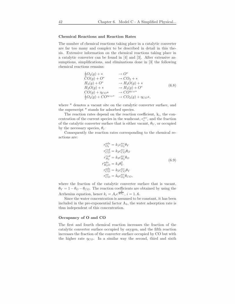
Chemical Reactions and Reaction Rates
The number of chemical reactions taking place in a catalytic converterare far too many and complex to be described in detail in this the-sis. Extensive information on the chemical reactions taking place ina catalytic converter can be found in [4] and [3]. After extensive as-sumptions, simplifications, and eliminations done in [3] the followingchemical reactions remains:
12O2(g) + ∗ → O∗
CO(g) + O∗ → CO2 + ∗H2(g) +O∗ → H2O(g) + ∗H2O(g) + ∗ → H2(g) +O∗
CO(g) + ηCO∗ → COηCO∗
12O2(g) + COηCO∗ → CO2(g) + ηCO∗,
(6.8)
where * denotes a vacant site on the catalytic converter surface, andthe superscript * stands for adsorbed species.
The reaction rates depend on the reaction coefficient, ki, the con-centration of the current species in the washcoat, cwci , and the fractionof the catalytic converter surface that is either vacant, θV , or occupiedby the necessary species, θi.
Consequently the reaction rates corresponding to the chemical re-actions are:
radsO2= k1c
wcO2θV
rredCO = k2cwcCOθO
rredH2= k3c
wcH2θO
radsH2O = k4θ2V
radsCO = k5cwcCOθV
roxCO = k6cwcO2θCO,
(6.9)
where the fraction of the catalytic converter surface that is vacant,θV = 1− θO− θCO. The reaction coefficients are obtained by using the
Arrhenius equation, hence ki = Aie−EiℜTs , i = 1..6.
Since the water concentration is assumed to be constant, it has beenincluded in the pre-exponential factor A4, the water adsorption rate isthus independent of this concentration.
Occupancy of O and CO
The first and fourth chemical reaction increases the fraction of thecatalytic converter surface occupied by oxygen, and the fifth reactionincreases the fraction of the converter surface occupied by CO but withthe higher rate ηCO. In a similar way the second, third and sixth
6.1. Model 43
reaction decreases the fraction of the converter surface occupied by thespecies in question.
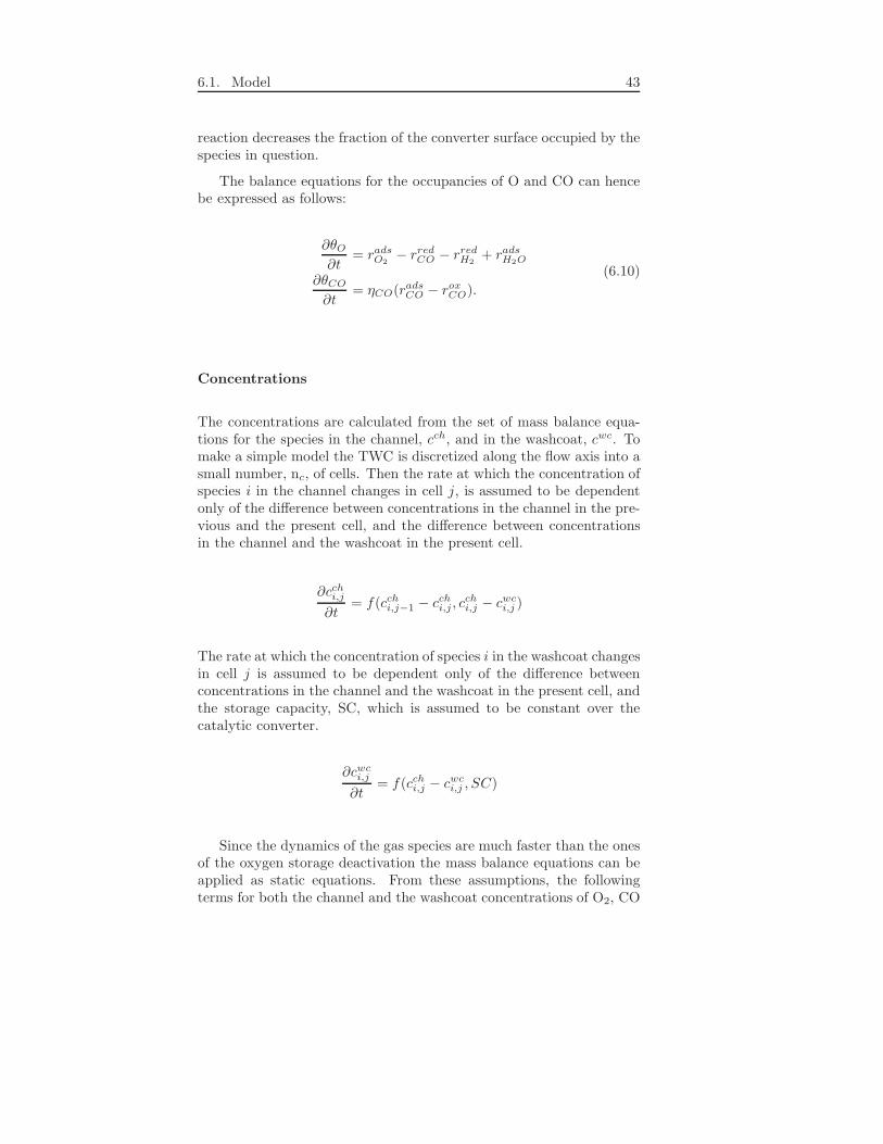
The balance equations for the occupancies of O and CO can hencebe expressed as follows:
∂θO∂t
= radsO2− rredCO − rredH2
+ radsH2O
∂θCO∂t
= ηCO(radsCO − roxCO).
(6.10)
Concentrations
The concentrations are calculated from the set of mass balance equa-tions for the species in the channel, cch, and in the washcoat, cwc. Tomake a simple model the TWC is discretized along the flow axis into asmall number, nc, of cells. Then the rate at which the concentration ofspecies i in the channel changes in cell j, is assumed to be dependentonly of the difference between concentrations in the channel in the pre-vious and the present cell, and the difference between concentrationsin the channel and the washcoat in the present cell.
∂cchi,j∂t
= f(cchi,j−1 − cchi,j , cchi,j − cwci,j )
The rate at which the concentration of species i in the washcoat changesin cell j is assumed to be dependent only of the difference betweenconcentrations in the channel and the washcoat in the present cell, andthe storage capacity, SC, which is assumed to be constant over thecatalytic converter.
∂cwci,j∂t
= f(cchi,j − cwci,j , SC)
Since the dynamics of the gas species are much faster than the onesof the oxygen storage deactivation the mass balance equations can beapplied as static equations. From these assumptions, the followingterms for both the channel and the washcoat concentrations of O2, CO
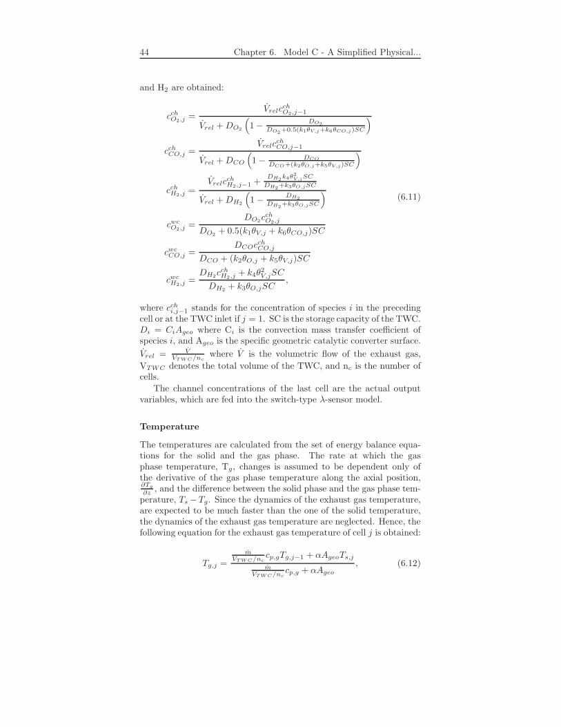
44 Chapter 6. Model C - A Simplified Physical...
and H2 are obtained:
cchO2,j =Vrelc
chO2,j−1
Vrel +DO2
(
1 −DO2
DO2+0.5(k1θV,j+k6θCO,j)SC
)
cchCO,j =Vrelc
chCO,j−1
Vrel +DCO
(
1 − DCO
DCO+(k2θO,j+k5θV,j)SC
)
cchH2,j =Vrelc
chH2,j−1 +
DH2k4θ
2V,jSC
DH2+k3θO,jSC
Vrel +DH2
(
1 −DH2
DH2+k3θO,jSC
)
cwcO2,j =DO2
cchO2,j
DO2+ 0.5(k1θV,j + k6θCO,j)SC
cwcCO,j =DCOc
chCO,j
DCO + (k2θO,j + k5θV,j)SC
cwcH2,j =DH2
cchH2,j+ k4θ
2V,jSC
DH2+ k3θO,jSC
,
(6.11)
where cchi,j−1 stands for the concentration of species i in the precedingcell or at the TWC inlet if j = 1. SC is the storage capacity of the TWC.Di = CiAgeo where Ci is the convection mass transfer coefficient ofspecies i, and Ageo is the specific geometric catalytic converter surface.
Vrel = VVT WC/nc
where V is the volumetric flow of the exhaust gas,
VTWC denotes the total volume of the TWC, and nc is the number ofcells.
The channel concentrations of the last cell are the actual outputvariables, which are fed into the switch-type λ-sensor model.
Temperature
The temperatures are calculated from the set of energy balance equa-tions for the solid and the gas phase. The rate at which the gasphase temperature, Tg, changes is assumed to be dependent only ofthe derivative of the gas phase temperature along the axial position,∂Tg
∂z , and the difference between the solid phase and the gas phase tem-perature, Ts−Tg. Since the dynamics of the exhaust gas temperature,are expected to be much faster than the one of the solid temperature,the dynamics of the exhaust gas temperature are neglected. Hence, thefollowing equation for the exhaust gas temperature of cell j is obtained:
Tg,j =
mVT WC/nc
cp,gTg,j−1 + αAgeoTs,jm
VT WC/nccp,g + αAgeo
, (6.12)
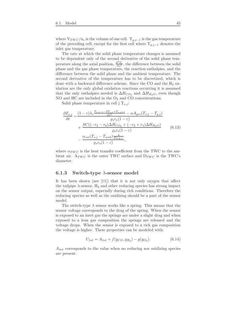
6.1. Model 45
where VTWC/nc is the volume of one cell. Tg,j−1 is the gas temperatureof the preceding cell, except for the first cell where Tg,j−1 denotes theinlet gas temperature.
The rate at which the solid phase temperature changes is assumedto be dependent only of the second derivative of the solid phase tem-
perature along the axial position, ∂2Ts
∂z2 , the difference between the solidphase and the gas phase temperature, the reaction enthalpies, and thedifference between the solid phase and the ambient temperature. Thesecond derivative of the temperature has to be discretized, which isdone with a backward difference scheme. Since the CO and the H2 ox-idation are the only global oxidation reactions occurring it is assumedthat the only enthalpies needed is ∆HCO2
and ∆HH2O, even thoughNO and HC are included in the O2 and CO concentrations.
Solid phase temperature in cell j Ts,j :
∂Ts,j∂t
=(1 − ε)λs
Ts,j−1−2Ts,j+Ts,j+1
dz2 − αAgeo(Ts,j − Tg,j)
scs(1 − ε)
+SC((−r2 − r6)∆HCO2
+ (−r3 + r4)∆HH2O)
scs(1 − ε)
−αcat(Ts,j − Tamb)
4DT WC
scs(1 − ε),
(6.13)
where αTWC is the heat transfer coefficient from the TWC to the am-bient air. ATWC is the outer TWC surface and DTWC is the TWC’sdiameter.
6.1.3 Switch-type λ-sensor model
It has been shown (see [11]) that it is not only oxygen that affectthe tailpipe λ-sensor, H2 and other reducing species has strong impacton the sensor output, especially during rich conditions. Therefore thereducing species as well as the oxidizing should be a part of the sensormodel.
The switch-type λ sensor works like a spring. This means that thesensor voltage corresponds to the drag of the spring. When the sensoris exposed to an inert gas the springs are under a slight drag and whenexposed to a lean gas composition the springs are released and thevoltage drops. When the sensor is exposed to a rich gas compositionthe voltage is higher. These properties can be modeled with:
Uλst = Aλst + f(yCO, yH2) − g(yO2
). (6.14)
Aλst corresponds to the value when no reducing nor oxidizing speciesare present.
46 Chapter 6. Model C - A Simplified Physical...
An analysis in [3] has shown that the sensor output correspondswith the logarithm of the exhaust gas components. When exposed torich exhausts the sensitivity to H2 is dominating, however even thoughthere is no H2 present the sensor shows a higher input than when ex-posed to an inert gas. The sensor output also decreases with increasingtemperatures. A model that covers these considerations is:
Uλst = Aλst + EA,λst · e−EE,λst
ℜTtp · log10(1 +BλstyCO + CλstyH2)
− Fλst · log10(1 +DλstyO2). (6.15)
When the concentrations are zero the corresponding term should alsobecome zero and thus the 1 in the logarithmic expressions. The 1 alsoprevent the terms from becoming negative.
The exhaust gas in the real sensor is brought to a chemical equi-librium and thus the model cannot be applied to the concentrationsdirectly. The calculation of the equilibrium concentrations is very com-plex and a crude approximation is used. When the mixture is lean theconcentrations are:
yO2= max(ytpO2
− 0.5(ytpH2+ ytpCO), 0)
yCO = 0
yH2= 0
(6.16)
and a somewhat more complicated calculation when the inlet is rich:
yO2= 0
yCO = max(ytpCO − 2(1 − wλst)ytpO2
+ min(ytpH2− 2wλsty
tpO2, 0), 0)
yH2= max(ytpH2
− 2wλstytpO2
+ min(ytpCO − 2(1 − wλst)ytpO2, 0), 0).
(6.17)
It is assumed that CO has a higher inclination to react with the excessO2 as compared to H2 and the weighing factor wλst is introduced totake that into account. wλst was chosen as:
wλst =0.3ytpH2
0.3ytpH2+ ytpCO
. (6.18)
The response time of the sensor is much shorter than the dynamicsof the exhaust gas composition. Thus the sensor dynamics can beneglected and the presented algebraic model should be sufficient.
6.2 Parameter estimation
The model contains many parameters. Most of the physical parametershave been found in tables or in the data sheets of the catalytic con-verter. However, the parameters not found must be estimated. These
6.2. Parameter estimation 47
parameters are the switch-type λ-sensor specific parameters, the oxy-gen storage capacity and heat-transfer coefficient between the TWCand ambient, the kinetic parameters of the TWC and heat conductiv-ity in the solid phase.
If measurements of the concentrations downstream of the catalyticconverter are available, the λ-sensor parameters can be found separatelywhich makes the estimation of the rest of the parameters much easier.
Unfortunately, concentration measurements were not available inthe laboratory used for measurements in this thesis and therefore theparameters are quite hard to obtain.
6.2.1 Simplifications and assumption
To make the parameter estimation more accurate a few assumptionsand simplifications can be made to get better start values to use withthe estimation algorithm.
Obtaining the lean-related parameters in the λ-sensor model
When the engine has been running lean long enough to fill the TWCwith oxygen the downstream exhausts can be assumed to be the sameas the inlet gases, which means that the inlet concentrations can beapplied directly to the λ-sensor model. If assuming that Aλst has thesame value as in [3] a least-square optimization routine can be appliedand Dλst and Fλst can be obtained.
Bλst and Cλst ratio
A constant ratio between Bλst and Cλst can be assumed. This ratio isassumed to be the same as in [3]
Fixed heat transfer and heat conduction
The heat transfer coefficient between the converter and the ambientair, αcat, can at first be set to zero. This will make the temperaturesincrease but the change is not dramatic. The heat conduction λs isimportant, though a high accuracy is not needed due to the fact thatthe model is very simplified. Hence a reasonable value can be used.
6.2.2 Estimation algorithm
Many of the parameters that has to be estimated are dependent on eachother and therefore an estimation algorithm has been made in order toget as accurate parameter values as possible. The optimization algo-rithm needs good first guesses. The algorithm should first be appliedto the kinetic parameters, SC, Bλst, EA,λst and EEλst with the rest
48 Chapter 6. Model C - A Simplified Physical...
of the values as suggested in section 6.2.1. Now the parameters havebeen narrowed down from 22 to 16. Next step is to freeze a few of theparameters at the time and apply the algorithm to the rest. This isdone in order to make the parameters which are dependent on otherparameters evolve without interacting with each other. An example ofthe estimation algorithm is given below:
1. kinetic parameters Ai and Ei, SC, Bλst, EA,λst and EEλst
2. kinetic parameters only
3. Bλst, EA,λst and EEλst only
4. SC only
5. all parameters, including Aλst, Cλst, Dλst, Fλst, αcat, λs
6. kinetic parameters only
7. sensor parameters only
8. αcat
9. SC
10. λs
The parameters are obtained by minimizing the error between themodel output and the switch-type λ-sensor. Some parameters how-ever, e.g αcat, affects the temperature rather than the model output,hence when αcat is estimated the least-square algorithm should mini-mize the error between the models temperature in the TWC and thesensor value instead of the switch-type λ-sensor.
If the result is not satisfying or if no good initial values are availablethe steps should of course be repeated.
The values obtained can be found in appendix C.
6.3 Validation
Two sets of parameters are presented in this chapter. The first set givesan output which is more alike the λ-sensor output than the second set,at least in the beginning of the simulations. The second set gives thestates a more realistic appearance than the first. The major differencebetween the first and second parameter set is that a parameter repre-senting the lambda offset had a fix value in the second set but not inthe first, when estimating the parameters.
The parameters (from both sets) have initially been obtained asdescribed above. The steps have been repeated several times.
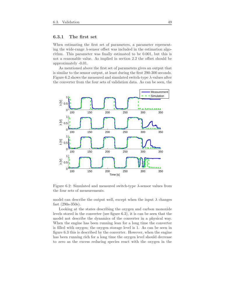
6.3. Validation 49
6.3.1 The first set
When estimating the first set of parameters, a parameter represent-ing the wide-range λ-sensor offset was included in the estimation algo-rithm. This parameter was finally estimated to be 0.001, but this isnot a reasonable value. As implied in section 2.2 the offset should beapproximately -0.01.
As mentioned above the first set of parameters gives an output thatis similar to the sensor output, at least during the first 290-300 seconds.Figure 6.2 shows the measured and simulated switch-type λ-values afterthe converter from the four sets of validation data. As can be seen, the
100 150 200 250 300 3500
0.5
1
λ [V
]
100 150 200 250 300 3500
0.5
1
λ [V
]
100 150 200 250 300 3500
0.5
1
λ [V
]
100 150 200 250 300 3500
0.5
1
λ [V
]
Time [s]
MeasurementSimulation
Figure 6.2: Simulated and measured switch-type λ-sensor values fromthe four sets of measurements.
model can describe the output well, except when the input λ changesfast (290s-350s).
Looking at the states describing the oxygen and carbon monoxidelevels stored in the converter (see figure 6.3), it is can be seen that themodel not describe the dynamics of the converter in a physical way.When the engine has been running lean for a long time the converteris filled with oxygen; the oxygen storage level is 1. As can be seen infigure 6.3 this is described by the converter. However, when the enginehas been running rich for a long time the oxygen level should decreaseto zero as the excess reducing species react with the oxygen in the
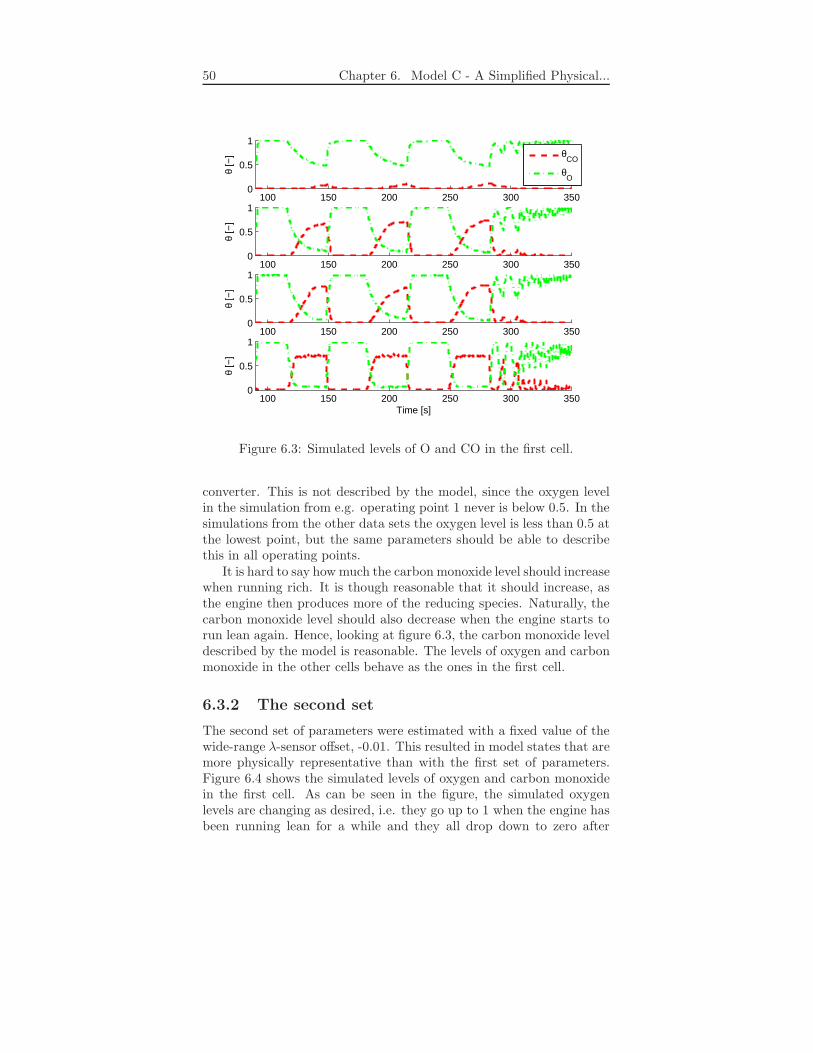
50 Chapter 6. Model C - A Simplified Physical...
100 150 200 250 300 3500
0.5
1
θ [−
]
100 150 200 250 300 3500
0.5
1
θ [−
]
100 150 200 250 300 3500
0.5
1
θ [−
]
100 150 200 250 300 3500
0.5
1
θ [−
]
Time [s]
θCO
θO
Figure 6.3: Simulated levels of O and CO in the first cell.
converter. This is not described by the model, since the oxygen levelin the simulation from e.g. operating point 1 never is below 0.5. In thesimulations from the other data sets the oxygen level is less than 0.5 atthe lowest point, but the same parameters should be able to describethis in all operating points.
It is hard to say how much the carbon monoxide level should increasewhen running rich. It is though reasonable that it should increase, asthe engine then produces more of the reducing species. Naturally, thecarbon monoxide level should also decrease when the engine starts torun lean again. Hence, looking at figure 6.3, the carbon monoxide leveldescribed by the model is reasonable. The levels of oxygen and carbonmonoxide in the other cells behave as the ones in the first cell.
6.3.2 The second set
The second set of parameters were estimated with a fixed value of thewide-range λ-sensor offset, -0.01. This resulted in model states that aremore physically representative than with the first set of parameters.Figure 6.4 shows the simulated levels of oxygen and carbon monoxidein the first cell. As can be seen in the figure, the simulated oxygenlevels are changing as desired, i.e. they go up to 1 when the engine hasbeen running lean for a while and they all drop down to zero after
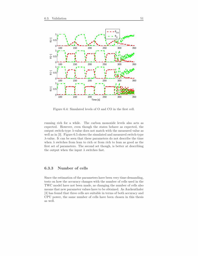
6.3. Validation 51
100 150 200 250 300 3500
0.5
1
θ [−
]
100 150 200 250 300 3500
0.5
1θ
[−]
100 150 200 250 300 3500
0.5
1
θ [−
]
100 150 200 250 300 3500
0.5
1
θ [−
]
Time [s]
θCO
θO
Figure 6.4: Simulated levels of O and CO in the first cell.
running rich for a while. The carbon monoxide levels also acts asexpected. However, even though the states behave as expected, theoutput switch-type λ-value does not match with the measured value aswell as in [3]. Figure 6.5 shows the simulated and measured switch-typeλ-value. It can be seen that these parameters do not describe the timewhen λ switches from lean to rich or from rich to lean as good as thefirst set of parameters. The second set though, is better at describingthe output when the input λ switches fast.
6.3.3 Number of cells
Since the estimation of the parameters have been very time-demanding,tests on how the accuracy changes with the number of cells used in theTWC model have not been made, as changing the number of cells alsomeans that new parameter values have to be obtained. As Auckenthaler[3] has found that three cells are suitable in terms of both accuracy andCPU power, the same number of cells have been chosen in this thesisas well.
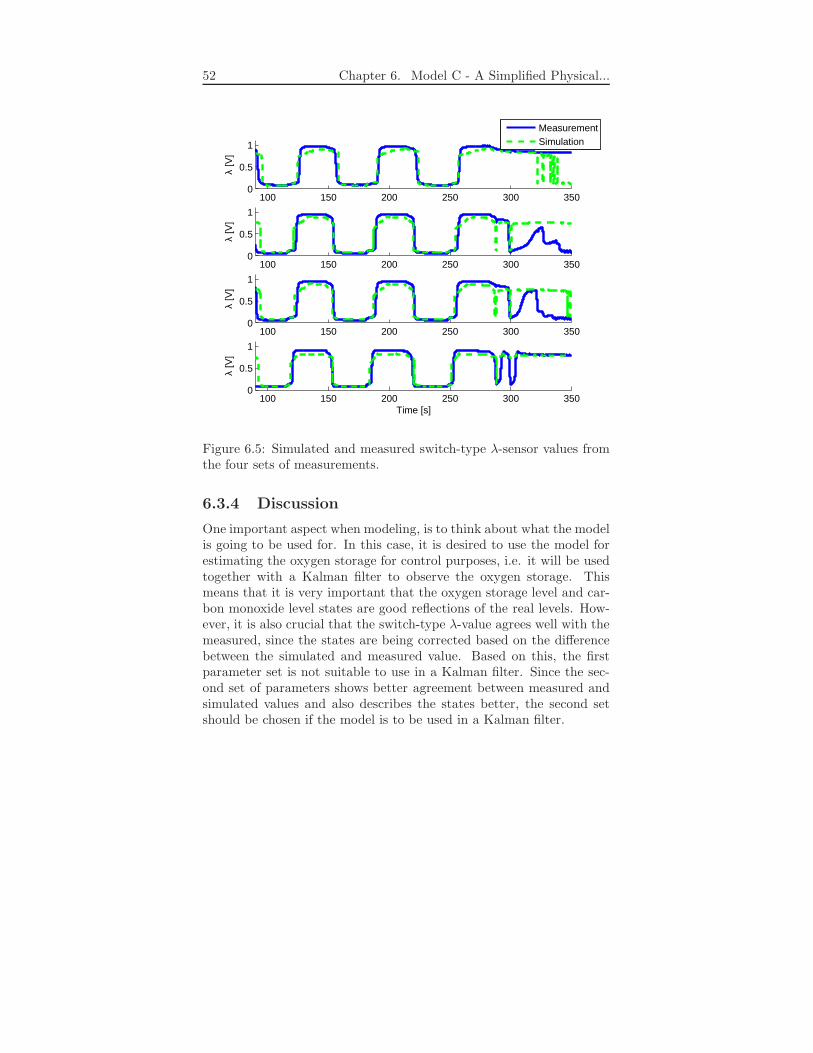
52 Chapter 6. Model C - A Simplified Physical...
100 150 200 250 300 3500
0.5
1
λ [V
]
100 150 200 250 300 3500
0.5
1
λ [V
]
100 150 200 250 300 3500
0.5
1
λ [V
]
100 150 200 250 300 3500
0.5
1
λ [V
]
Time [s]
MeasurementSimulation
Figure 6.5: Simulated and measured switch-type λ-sensor values fromthe four sets of measurements.
6.3.4 Discussion
One important aspect when modeling, is to think about what the modelis going to be used for. In this case, it is desired to use the model forestimating the oxygen storage for control purposes, i.e. it will be usedtogether with a Kalman filter to observe the oxygen storage. Thismeans that it is very important that the oxygen storage level and car-bon monoxide level states are good reflections of the real levels. How-ever, it is also crucial that the switch-type λ-value agrees well with themeasured, since the states are being corrected based on the differencebetween the simulated and measured value. Based on this, the firstparameter set is not suitable to use in a Kalman filter. Since the sec-ond set of parameters shows better agreement between measured andsimulated values and also describes the states better, the second setshould be chosen if the model is to be used in a Kalman filter.
Chapter 7
Model comparison
One reason to compare the models is to decide whether any of themodels can be used in the online adaption strategy described in thefollowing chapter.
7.1 Accuracy of the models
An important aspect when comparing the models is their accuracycompared to measurements.
Model A
It is hard to draw any conclusions about the accuracy of the catalyticconverter model in chapter 4, since a reliable wide-range λ-sensor down-stream of the converter, or a λ converter model with high accuracy isneeded to compare the model with measured data.
With the λ converter used in this thesis, the model of the converterseems to capture the dynamics of the converter well for one operatingpoint, but the model is not expected to show as good results when theoperating point is changed or the converter is aged.
Model B
Since no simulations has been done with this model there is no infor-mation available about the accuracy of the model.
Model C
The accuracy of the Model C output as compared to measurementsis good, regarding the low complexity of the model. It describes thelong-period changes in inlet λ well, but the agreement when the inlet λ
53
54 Chapter 7. Model comparison
changes fast is not very good. The oxygen level and carbon monoxidestates changes in a reasonable way.
Comparison
The accuracy of Model A and Model C is almost the same, as canbe seen in figures 4.3 and 6.5. The accuracy of Model C is thoughexpected to be better than Model A in other operating points thanused for evaluation in this thesis, since the model is based on physicalreactions in the converter.
7.2 Inputs and outputs
Due to economical reasons, automotive producers is reluctant to addadditional sensors. Therefore a model using only the present sensors isdesirable.
Model A
The catalytic converter model described in chapter 4, uses measure-ments from a wide-range λ-sensor before the catalytic converter, andthe fuel mass flow as inputs. The output, which is to be compared withmeasurements, from the model of the catalytic converter is a wide-rangeλ-value. When the λ-converter model is applied however, a switch-typeλ-value is the output. The λ-converter model also needs exhaust gastemperature as input.
Model B
Model B takes the upstream wide-range λ as input and the output isthe downstream wide-range λ.
Model C
Model C takes the wide-range λ, exhaust mass flow and exhaust tem-perature as inputs. The output is a switch-type λ-value.
Comparison
The major difference in the models’ need for extra sensors, is the useof a wide-range or a switch-type λ-sensor downstream of the converter.The measurements of the mass flow and exhaust gas temperatures areof minor concerns. Hence, from this point of view, Model A and C arepreferred.
7.3. Number of states and parameters 55
7.3 Number of states and parameters
The number of parameters is important because a higher number in-dicates that a good estimation of the parameters is harder to obtain.This in turn makes it hard to apply and adjust the model to differentcatalytic converters.
The number of states is a measurement of how detailed the modelis. Additionally the CPU recourses demanded by an online adaptionstrategy, such as the one described in chapter 8, is linked to the numberof states together with the number of parameters that changes as aresult of the ageing of the converter.
Model A
Model A contains two states describing the oxygen storage and the re-versible catalyst deactivation. These correspond to the states in ModelC describing the occupancy of O and CO. A big difference is that noconsideration has been made to describe the spatially distributed na-ture of the converter in this model.
The model of the catalytic converter contains nine parameters. Ad-ditionally the λ converter introduce ten parameters that have to beestimated. Among the nine parameters in the model of the converterthere are six which change as the catalytic converter ages.
Model B
Model B has only one state, which indicates the current global rela-tive oxygen coverage of ceria (ROC) in the catalytic converter. ROCcorresponds to the storage capacity SC in Model C. Model B has twofunctions that easily can be estimated with a data set where the ROCgoes from 0 to 1 and from 1 to 0. Furthermore, the model has oneadditional parameter that has to be estimated. This parameter is easyto obtain using the same data sets as for the functions. Both parame-ter and functions change over time and can be estimated online. Goodsensor values must be available in order to estimate the parameter andfunctions.
Model C
The dynamics of the converter is in Model C described by the TWCmodel. Each cell in the TWC model contains three states, describingthe occupancy of O and CO, and the solid phase temperature. In thiscase when the catalytic converter is divided into three cells there areconsequently nine states.
56 Chapter 7. Model comparison
The exhaust gas model, the TWC model and the sensor model havetogether 22 parameters which need to be estimated. Amongst themthere is one which changes as the catalytic converter ages.
Comparison
The number of parameters that need to be estimated are 19 in Model A,1 in Model B, and 22 in Model C. Model B additionally contains 2 func-tions with parameters, but these are obtained by simple calculations,and does not demand any optimization. Estimating the parameters inModel A and Model C, is hence expected to cause more trouble, thanthe estimation for Model B.
In an online strategy two states and 6 parameters would have to beestimated if Model A was to be used. One state, the parameter andtwo functions would have to be estimated if using Model B. The samenumbers for Model C is 9 states and one parameter. From this, theconclusion that Model B is least demanding if it were to be implementedin an online strategy, is drawn.
7.4 Simulation speed
The time it takes to simulate the models is a measurement of theircomplexity. The shorter time it takes, the easier the model will beto fit into an engine control system. Tests have shown that a 240 slong measurement sequence takes approximately 9 seconds to simulatewith Model C and approximately 4 seconds with Model A. This is nota surprising result since Model A has fewer states than Model C andhence should not need as much computer calculations as Model C.
7.5 Extensibility
The requirements of the models might differ depending on the field ofapplication. It is therefore desirable to know in what extent the modelscan be modified or extended.
Model A
Model A is empirical, and the dynamics of the TWC is assumed to bedominated of the oxygen storage and the reversible catalyst deactiva-tion. Extending this model with further characteristics would probablyresult in the need to reconsider the entire model.
7.6. Final comparison 57
Model B
The model can easily be extended to be accurate in a wider operatingrange by making the parameter and functions depend on the exhaustmass flow. However, that also means that the model needs one moreinput.
Model C
Since Model C is a simplified physical model, it is quite easy to extend.One way is to include humid air or a gasoline containing not only Hand C, but also O in the combustion reactions (6.1) and (6.2).
It is also likely that the model can be extended with the NO andHC concentrations without a drastic increase of the CPU power.
Comparison
Model C originates from a more advanced model, which has been sim-plified in order to be used in control strategies or on board diagnostics.More about the advanced model can be read in [3]. It is hence quiteeasy to extend. Even though Model B is a black-box model, it can beextended to show better results with different mass flows.
7.6 Final comparison
The most important aspect when comparing the models, is of coursethe accuracy compared to measurements. If the model makes a poordescription of the catalytic converter, it does not matter if e.g. thedemand for CPU power is limited.
Model B has due to offset problems with the sensors not been im-plemented and thus it cannot be used in the online adaptation strategy.
Model C is expected to be more accurate than Model A in otheroperating point than the ones used in this thesis.
Model C contains the highest amount of states, and is hence themost CPU consuming model. Additionally it is the model where theparameter values are hardest to obtain. On the other hand, the manystates and parameters make the model more reliable when it comes todescribing the behavior of the catalytic converter, and Model C has themost physical interpretation of the three models.

58
Chapter 8
Extended Kalman filter
To be able to use the models of the catalytic converter from the previouschapters, both the estimation of the internal state variables, by meansof an observer, and the estimation of the parameters that changes overthe converter’s lifetime, should be performed by the control unit duringoperation, i.e. an online adaption strategy is required.
The correct estimation of the controlled internal state variables suchas the oxygen storage level require a fast and accurate adaption to the”true” values. One way to achieve this is to use an extended Kalmanfilter (EKF), which can handle both the internal state variables andadapting parameters, as well as the nonlinear models.
8.1 Introduction to EKF
The EKF in this chapter is implemented accordingly to the EKF pre-sented in [3]. Therefore, only a short introduction is given. For furtherinformation on the subject the reader is referred to [3], and books andpapers on the subject such as [5] and [13].
Assume that the process noise and the measurement noise pro-cesses are uncorrelated, zero-mean white noise and additive to the statederivative and the output vectors. Then the system can be describedby nonlinear state space equations:
x = f(x,u) + w
y = h(x,u) + v,
where u is the control input vector, x the state vector, y the outputvector, w the process noise and v the measurement noise. The co-variance matrices for the process and the measurement noise can be
59
60 Chapter 8. Extended Kalman filter
expressed as:
Q = E[wwT ]
R = E[vvT ],
and the covariance matrix of the estimate error as:
P = E[(x − x)(x − x)T ].
The model has to be linearized around the current state estimate x
to obtain the systems measurement matrix H:
H =∂h(x,u)
∂x
∣
∣
∣
∣
x=x
and the dynamics matrix F:
F =∂f(x,u)
∂x
∣
∣
∣
∣
x=x
.
Since the purpose is to create a discrete filter, the fundamental matrixΦk is required instead of the systems dynamic matrix. Φk can beapproximated by the first two terms of the Taylor-series expansion:
Φk = eFhs ≈ I + Fhs
The first step of the extended Kalman filter algorithm is the ”timeupdate” or ”extrapolation” step, where the state vector estimate x andthe covariance matrix P are projected one step ahead:
x−
k = f(xk−1,uk−1) (8.1a)
P−
k = ΦkPk−1ΦTk + Qk, (8.1b)
where the discrete process noise matrix Qk can be obtained from thecontinuous matrix Q by integration over one time step:
Qk =
∫ khs
(k−1)hs
Φ(τ)QΦT (τ)dτ
The second step is the ”measurement update” or ”correction” step,where the state vector estimate x and the covariance matrix P arecorrected using the error between the projected output vector h(x−
k )and the measured vector zk, and the measurement matrix Hk:
xk = x−
k + Kk(zk − h(x−
k ,uk)) (8.2a)
Pk = (I − KkHk)P−
k (8.2b)
8.2. Implementation 61
The Kalman gain Kk is calculated from the discrete Riccati-equation:
Kk = P−
k HTk (HkP
−
k HTk + Rk)
−1 (8.3)
The filter algorithm is established with equations (8.1)-(8.3). Theseequations needs to be calculated every time step. Hence, the amount ofCPU power that is needed to carry them out has to be rather small.With this in mind, one might think that what appears to be a matrixinversion in the Riccati equation (8.3) could cause problems, but acloser inspection reveals that this is actually a scalar inversion, in thiscase, since the output vector is one dimensional. (Bara en utsignal)
8.1.1 Parameter identification
The parameters that changes over the catalytic converter’s lifetime needto be identified online. This is easily implemented when a discrete EKFis used by seeing them as additional state variables.
The discrete state space equation is originally expressed as:
xk+1 = f(xk,uk) + wk
yk = h(xk,uk) + vk,
and then augmented with the equation for the new state variables
pk+1 = pk + wp,k,
where p denotes the vector with the new state variables and wp,k isa zero-mean scalar white noise process. The effect of this is that p
is kept constant in the extrapolation step and only adjusted in themeasurement update step. Obviously Q and P have to be augmentedaccordingly.
8.2 Implementation
In this thesis, as well as in [3], the model incorporated in the EKF isthe Model C.
As a discrete EKF is used, the model has to be discretized. Oneway to do this is to approximate the expressions for the states in thecatalytic converter model with an Euler forward scheme.
When using Model C, the input, state and output vectors are de-
62 Chapter 8. Extended Kalman filter
fined as follows:
u =
λmexh
Texh
, x =
θO,1θCO,1Ts,1θO,2θCO,2Ts,2θO,3θCO,3Ts,3
, y = [Uλst]
The discrete form of the state space model is augmented with theparameter that needs to be identified, SC, which is the parameter thatchanges as the converter ages:
SCk+1 = SCk + wSC,k
Hence the model now contains ten state variables. This is close tothe allowed upper limit. As stated before it should be simple enoughto fit in the control system.
Since the coupling between the temperatures and the sensor out-put is relatively weak the filter can be simplified by not including thetemperatures in the measurement update step. The temperatures arehence only calculated in the extrapolation step and then handled asmodel parameters.
The state vector can thus be split in two vectors
xcorr =
θO,1θCO,1θO,2θCO,2θO,3θCO,3SC
and xTemp =
Ts,1Ts,2Ts,3
.
These two vectors in combination is used with an Euler forward schemeto calculate the state vector in the extrapolation step, but only xcorris updated in the correction step.
An attempt to calculate the Jacobians F and H analytically wasmade, but this task turned out to be to awkward, and they are herecalculated numerically with a forward differential scheme.
8.3 Tuning of the EKF
The two covariance matrices Q and R are used as tuning parameters ofthe EKF. If R is chosen large as compared to Q, the measured value is
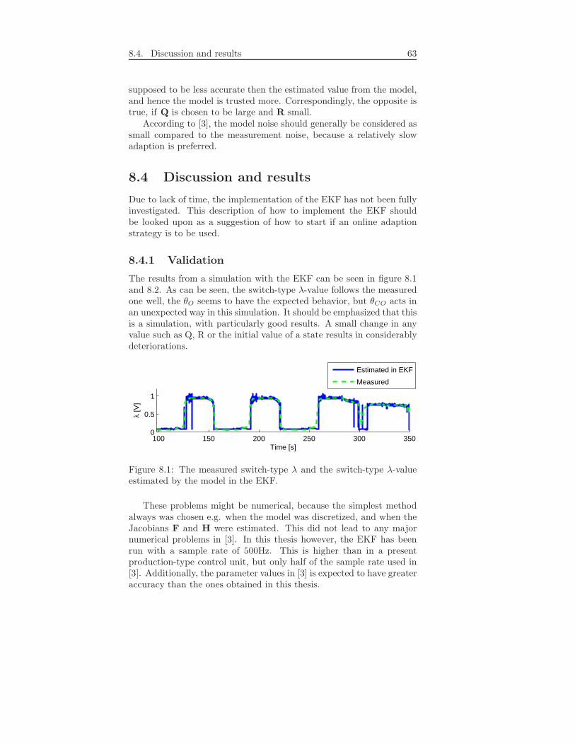
8.4. Discussion and results 63
supposed to be less accurate then the estimated value from the model,and hence the model is trusted more. Correspondingly, the opposite istrue, if Q is chosen to be large and R small.
According to [3], the model noise should generally be considered assmall compared to the measurement noise, because a relatively slowadaption is preferred.
8.4 Discussion and results
Due to lack of time, the implementation of the EKF has not been fullyinvestigated. This description of how to implement the EKF shouldbe looked upon as a suggestion of how to start if an online adaptionstrategy is to be used.
8.4.1 Validation
The results from a simulation with the EKF can be seen in figure 8.1and 8.2. As can be seen, the switch-type λ-value follows the measuredone well, the θO seems to have the expected behavior, but θCO acts inan unexpected way in this simulation. It should be emphasized that thisis a simulation, with particularly good results. A small change in anyvalue such as Q, R or the initial value of a state results in considerablydeteriorations.
100 150 200 250 300 3500
0.5
1
Time [s]
λ [V
]
Estimated in EKF
Measured
Figure 8.1: The measured switch-type λ and the switch-type λ-valueestimated by the model in the EKF.
These problems might be numerical, because the simplest methodalways was chosen e.g. when the model was discretized, and when theJacobians F and H were estimated. This did not lead to any majornumerical problems in [3]. In this thesis however, the EKF has beenrun with a sample rate of 500Hz. This is higher than in a presentproduction-type control unit, but only half of the sample rate used in[3]. Additionally, the parameter values in [3] is expected to have greateraccuracy than the ones obtained in this thesis.
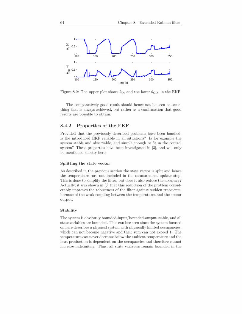
64 Chapter 8. Extended Kalman filter
100 150 200 250 300 3500
0.5
1
θ O [−
]
100 150 200 250 300 3500
0.5
1
Time [s]
θ CO
[−]
Figure 8.2: The upper plot shows θO, and the lower θCO, in the EKF.
The comparatively good result should hence not be seen as some-thing that is always achieved, but rather as a confirmation that goodresults are possible to obtain.
8.4.2 Properties of the EKF
Provided that the previously described problems have been handled,is the introduced EKF reliable in all situations? Is for example thesystem stable and observable, and simple enough to fit in the controlsystem? These properties have been investigated in [3], and will onlybe mentioned shortly here.
Splitting the state vector
As described in the previous section the state vector is split and hencethe temperatures are not included in the measurement update step.This is done to simplify the filter, but does it also reduce the accuracy?Actually, it was shown in [3] that this reduction of the problem consid-erably improves the robustness of the filter against sudden transients,because of the weak coupling between the temperatures and the sensoroutput.
Stability
The system is obviously bounded-input/bounded-output stable, and allstate variables are bounded. This can bee seen since the system focusedon here describes a physical system with physically limited occupancies,which can not become negative and their sum can not exceed 1. Thetemperature can never decrease below the ambient temperature and theheat production is dependent on the occupancies and therefore cannotincrease indefinitely. Thus, all state variables remain bounded in the
8.4. Discussion and results 65
real system and since the model is a representation of the reality, theyremain bounded in the model as well. According to [3], the resultinglinearized system is asymptotically stable in any steady state operatingpoint.
When the model is implemented in an EKF however, it is possiblethat the states is adjusted to values outside their physical limitations.One way to try to come around this is to implement boundaries inthe EKF, which also has been done. This might be another reason tothe strange behavior of θCO, since it primarily occurs when there issupposed to be higher levels of θCO.
Observability
To investigate the observability, a comparison between the model con-sisting of three connected cells and two occupancies, and a system ofthree tanks filled with e.g. water and oil, is made in [3]. If each tankleaks water/oil to the next tank dependent on the level of the liquid,and the size and geometry of the tanks are known, as well as the cor-relation of the storage levels and the leakage, it is intuitively obviousthat the levels of water and oil in the three tanks can be determined ifthe amount of water and oil leaving the last tank is measured.
Convergence
The investigation of the convergence is done in a similar way as withthe observability in [3]. A system consisting of a tank with entering andleaving mass flows is used to conclude that the system has to be excitedto guarantee convergence of the Kalman filter states to the ”true” val-ues. Under steady state conditions, when the input and output massflows are equal and constant, it is clear that the volume of the tankcannot be determined. In the model it is theoretically possible to de-termine the storage capacity under steady state conditions, since thereaction rates and hence both the heat production and the tailpipe con-centrations are dependent on SC. But this input-output link is weak.
The condition for convergence is hence that the system has to beexcited. This is however usually not a problem. The disturbances ofthe λ at the TWC inlet and the transients of the exhaust gas mass flowduring normal driving conditions are sufficient. The worst case scenariois when the driving is constant during longer periods, e.g. when drivingon a highway. In that case the excitations can become very weak, butat least the process does not diverge.

66
Chapter 9
Results and Discussion
The purpose of this thesis was to examine the possibilities to modelthe dynamics of a catalytic converter for control purposes. During thesearch for existing models, three promising models were found and theyhave been investigated in this thesis.
All three models have the wide-range λ as input and have at leastone state that in some way describes the oxygen storage level, and theyall consider catalyst deactivation. The three models are fairly simpleand needs online adaptation due to ageing of the converter. A shortsummary of the most important features of the models are presentedbelow. Further comparison of the models is given in chapter 7.
Two of the models (Model A and Model B) have a wide-range λas output. To be able to compare the values from these models withmeasurements, the wide-range λ-sensor downstream of the catalyticconverter have to be accurate enough. This is a problem since wide-range sensors often suffers from time varying biases. More about thedisadvantage of a wide-range sensor downstream of the converter canbe found in section 3.3. The third model (Model C), on the other hand,has a switch-type λ as output.
Of the three models, Model B would probably be the one that de-mands the least CPU power and it is the easiest one to adapt to dif-ferent kinds of converters. No expensive tests or optimization routineshave to be done to obtain the parameter and functions. However, itis also the most sensitive model by means of the characteristics of theλ-sensors. The dynamics in Model B is based on the wide-range sensorvalues before and after the converter, and when the sensors do not be-have as expected the model works poorly. The sensor problem is hardto get around, since an accurate converter model from switch-type towide-range λ-value is difficult to make, because of the nonlinearity ofthe switch-type sensor.
Model A describes the oxygen level well, but the λ-sensor value
67
68 Chapter 9. Results and Discussion
after the converter is not reliable, which is crucial if the model is to beused for control purposes. To overcome this, the original TWC modelhas been extended with a model that converts the output wide-range λinto a switch-type λ. This gives a better result, but it is not expectedto extrapolate to other operating points than the ones used for theparameter estimation.
Model C is the most detailed of the three models examined, it is thusno surprise that it is the most accurate, consume the highest amountof CPU power, and contains the highest number of parameters. Eventhough the results in this investigation is not as good as the resultsin [3], it is the most promising of the three models presented in thisthesis. The drawback of Model C is that it has many parameters thatare hard to estimate if only the switch-type λ-sensor is available formeasurements. If sensors measuring the concentrations of the speciesafter the converter are available, the parameter estimation can be di-vided into two parts, and thus the identification of the parameters iseasier.
The extended Kalman filter presented in chapter 8, together withModel C, is not fully investigated and should be considered as a way tostart if an online adaption strategy is to be implemented. The use ofan EKF is promising, and good results are expected if the previouslydescribed numerical problems (see section 8.4.1) are seen to.
An important conclusion drawn from this thesis, is that the behaviorof the sensors have to be taken into account if a model of the converteris to be used e.g. for onboard control.
Finally, the chances are good that the extended Kalman filter to-gether with Model C can successfully be used in an engine control sys-tem, if an effort is made to tune in the model parameters even betterand the problems with the EKF is solved.
Chapter 10
Future work
First of all, more time should be invested in obtaining parameter valuesfor Model C that describe the dynamics more accurately, e.g by usingother estimation algorithms or investigate if any simplifications like theones in section 6.2.1 can be done. When satisfying results have beenobtained, the next step is to solve the problems in the extended Kalmanfilter and finally, test the filter online with a control strategy. Since thestorage capacity is adapted online the filter can be used for diagnosticpurposes as well.
As described in previous chapters, the reactions taking place inthe converter make the gas composition change dynamically. As thegas composition has great impact on the sensors’ behavior, furtherinvestigation of the λ-sensors are highly recommended, especially ifa wide-range λ-sensor is to be used. Additionally, the effects of sensorageing should be examined.
69

70
References
[1] Division of vehicular systems, lab. Internet site.http://www.fs.isy.liu.se/Lab/, visited June 2005.
[2] Laborationskompendium grona bilen - reglerteknik for fordon. Labcompendium, Division of Vehicular Systems, Department of Elec-trical Engineering, Linkopings Universitet, Linkoping, Sweden,2004. In Swedish.
[3] T. Auckenthaler. Modelling and Control of Three-Way CatalyticConverters. Phd thesis, June 2005.
[4] Mario Balenovic. Modeling and Model-Based Control of a Three-Way Catalytic Converter. Phd thesis, Technische Univeriteit Eind-hoven, 2002.
[5] Lennart Ljung Fredrik Gustafsson and Mille Millnert. Signalbe-handling. Studentlitteratur, Lund, Sweden, 2 edition, 2001. InSwedish.
[6] James C. Peyton Jones. Modeling combined catalyst oxygen stor-age and reversible deactivation dynamics for improved emissionsprediction. SAE paper 2003-01-0999, 2003.
[7] James C. Peyton Jones. A novel approach to catalyst obd. SAEpaper 2005-01-0024, 2005.
[8] Kenneth R. Muske and James C. Peyton Jones. Feedfor-ward/feedback air fuel ratio control for an automotive catalyst. InProceedings of the American Control Conference, volume 2, pages1386–1391, Denver, Colorado, June 2003.
[9] Kenneth R. Muske and James C. Peyton Jones. Estimating theoxygen storage level of a three-way automotive catalyst. In Pro-ceedings of the American Control Conference, volume 5, pages 4060– 4065, Boston, Massachusetts, June 2004.
71
72 References
[10] Lars Nielsen and Lars Eriksson. Course material Vehicular Sys-tems. Linkoping, Sweden, 2004.
[11] Christopher H. Onder Theophil S. Auckenthaler and Hans P. Geer-ing. Aspects of dynamic three-way catalyst behaviour includingoxygen storage. In Proceedings of the IFAC Symposium on Ad-vances in Automotive Control, University of Salerno, Italy, April2004.
[12] Christopher H. Onder Theophil S. Auckenthaler and Hans P. Geer-ing. Online estimation of the oxygen storage level of a three-waycatalyst. SAE paper 2004-01-0525, 2004.
[13] Greg Welch and Gary Bishop. An introduction to the kalmanfilter. Technical Report TR 95-041, Department of Computer Sci-ence, University of North Carolina, Chapel Hill, US, April 2004.http://www.cs.unc.edu/∼welch/media/pdf/kalman intro.pdf,visited June 2005.
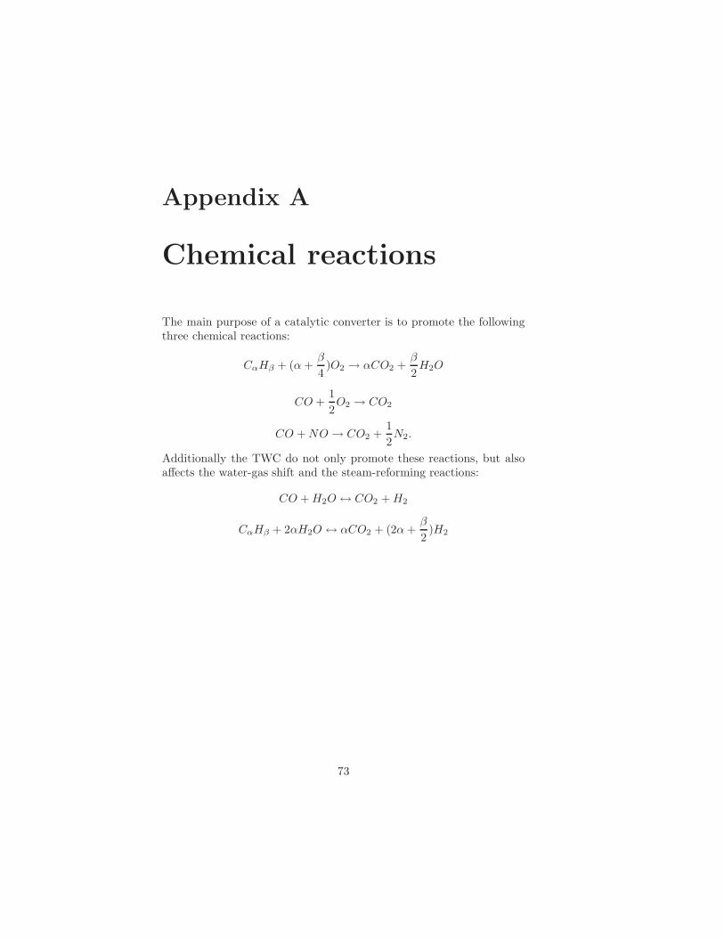
Appendix A
Chemical reactions
The main purpose of a catalytic converter is to promote the followingthree chemical reactions:
CαHβ + (α+β
4)O2 → αCO2 +
β
2H2O
CO +1
2O2 → CO2
CO +NO → CO2 +1
2N2.
Additionally the TWC do not only promote these reactions, but alsoaffects the water-gas shift and the steam-reforming reactions:
CO +H2O ↔ CO2 +H2
CαHβ + 2αH2O ↔ αCO2 + (2α+β
2)H2
73
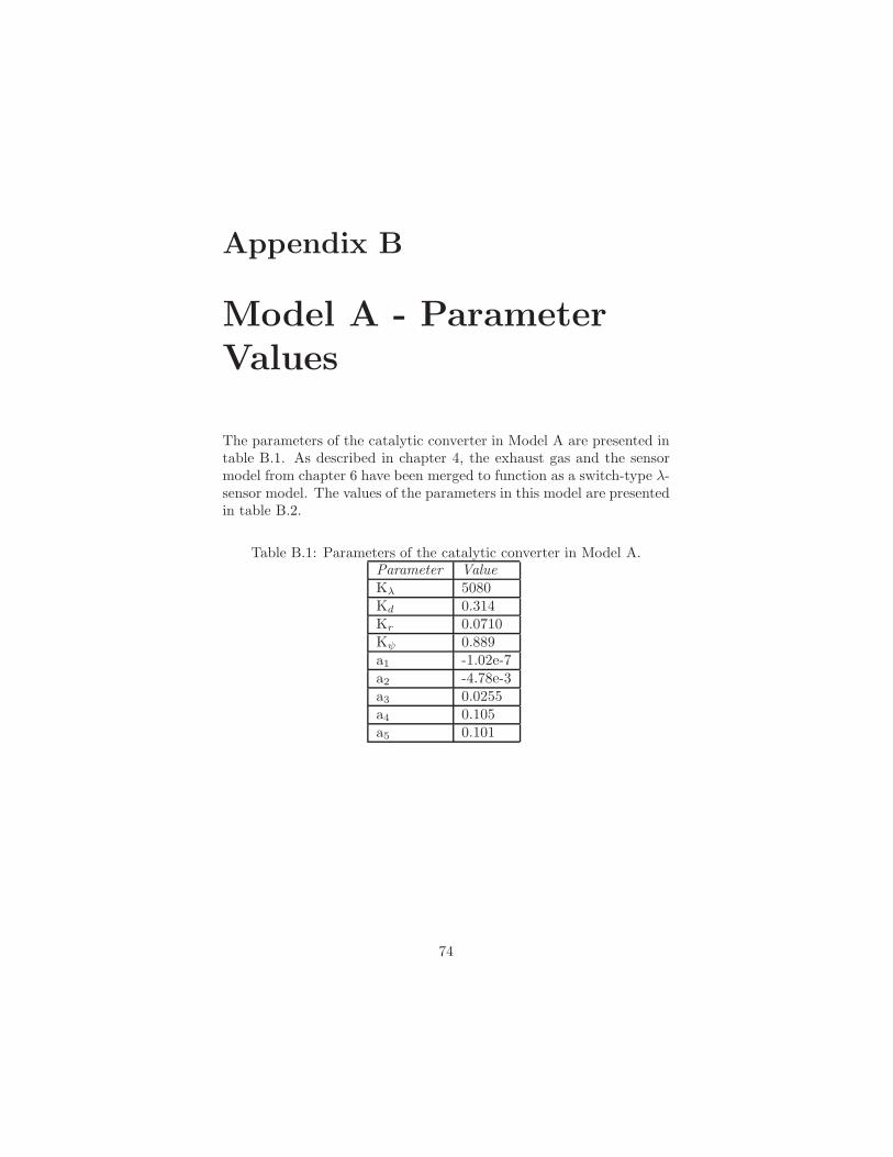
Appendix B
Model A - Parameter
Values
The parameters of the catalytic converter in Model A are presented intable B.1. As described in chapter 4, the exhaust gas and the sensormodel from chapter 6 have been merged to function as a switch-type λ-sensor model. The values of the parameters in this model are presentedin table B.2.
Table B.1: Parameters of the catalytic converter in Model A.Parameter ValueKλ 5080Kd 0.314Kr 0.0710Kψ 0.889a1 -1.02e-7a2 -4.78e-3a3 0.0255a4 0.105a5 0.101
74
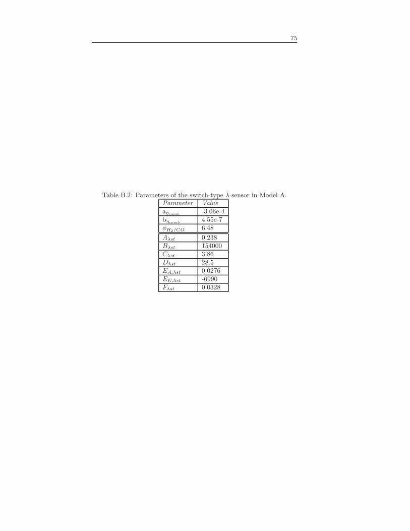
75
Table B.2: Parameters of the switch-type λ-sensor in Model A.Parameter Valueaηcomb
-3.06e-4bηcomb
4.55e-7φH2/CO 6.48
Aλst 0.238Bλst 154000Cλst 3.86Dλst 28.5EA,λst 0.0276EE,λst -6990Fλst 0.0328
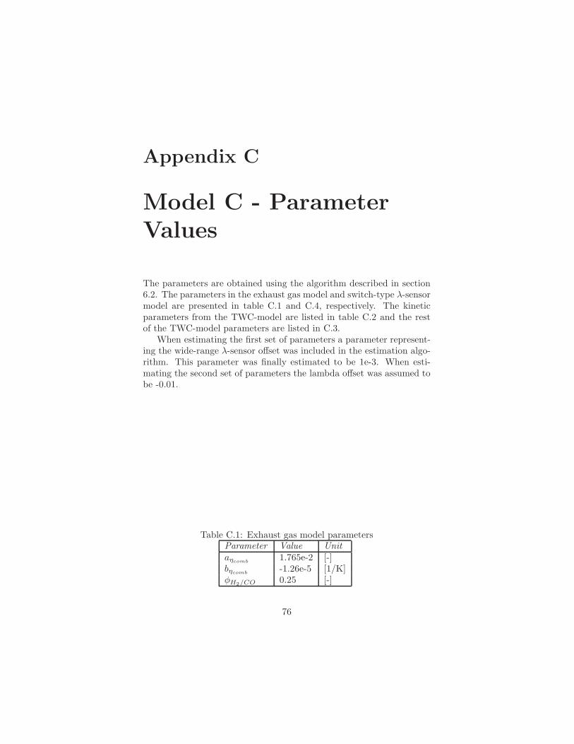
Appendix C
Model C - Parameter
Values
The parameters are obtained using the algorithm described in section6.2. The parameters in the exhaust gas model and switch-type λ-sensormodel are presented in table C.1 and C.4, respectively. The kineticparameters from the TWC-model are listed in table C.2 and the restof the TWC-model parameters are listed in C.3.
When estimating the first set of parameters a parameter represent-ing the wide-range λ-sensor offset was included in the estimation algo-rithm. This parameter was finally estimated to be 1e-3. When esti-mating the second set of parameters the lambda offset was assumed tobe -0.01.
Table C.1: Exhaust gas model parametersParameter Value Unitaηcomb
1.765e-2 [-]bηcomb
-1.26e-5 [1/K]φH2/CO 0.25 [-]
76
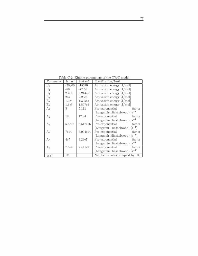
77
Table C.2: Kinetic parameters of the TWC modelParameter 1st set 2nd set Specification/UnitE1 -20000 -18310 Activation energy [J/mol]E2 -80 -77.56 Activation energy [J/mol]E3 2.2e5 2.214e5 Activation energy [J/mol]E4 2e5 2.23e5 Activation energy [J/mol]E5 1.3e5 1.395e5 Activation energy [J/mol]E6 1.6e5 1.597e5 Activation energy [J/mol]A1 5 5.111 Pre-exponential factor
(Langmuir-Hinshelwood) [s−1]A2 18 17.84 Pre-exponential factor
(Langmuir-Hinshelwood) [s−1]A3 5.5e16 5.517e16 Pre-exponential factor
(Langmuir-Hinshelwood) [s−1]A4 7e14 6.094e14 Pre-exponential factor
(Langmuir-Hinshelwood) [s−1]A5 4e7 4.23e7 Pre-exponential factor
(Langmuir-Hinshelwood) [s−1]A6 7.5e9 7.441e9 Pre-exponential factor
(Langmuir-Hinshelwood) [s−1]ηCO 12 Number of sites occupied by CO
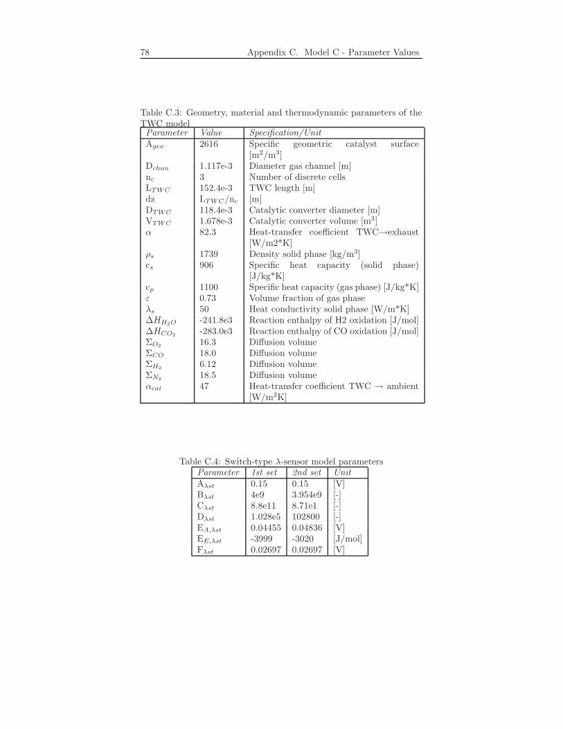
78 Appendix C. Model C - Parameter Values
Table C.3: Geometry, material and thermodynamic parameters of theTWC modelParameter Value Specification/UnitAgeo 2616 Specific geometric catalyst surface
[m2/m3]Dchan 1.117e-3 Diameter gas channel [m]nc 3 Number of discrete cellsLTWC 152.4e-3 TWC length [m]dz LTWC/nc [m]DTWC 118.4e-3 Catalytic converter diameter [m]VTWC 1.678e-3 Catalytic converter volume [m3]α 82.3 Heat-transfer coefficient TWC→exhaust
[W/m2*K]ρs 1739 Density solid phase [kg/m3]cs 906 Specific heat capacity (solid phase)
[J/kg*K]cp 1100 Specific heat capacity (gas phase) [J/kg*K]ε 0.73 Volume fraction of gas phaseλs 50 Heat conductivity solid phase [W/m*K]∆HH2O -241.8e3 Reaction enthalpy of H2 oxidation [J/mol]∆HCO2
-283.0e3 Reaction enthalpy of CO oxidation [J/mol]ΣO2
16.3 Diffusion volumeΣCO 18.0 Diffusion volumeΣH2
6.12 Diffusion volumeΣN2
18.5 Diffusion volumeαcat 47 Heat-transfer coefficient TWC → ambient
[W/m2K]
Table C.4: Switch-type λ-sensor model parametersParameter 1st set 2nd set UnitAλst 0.15 0.15 [V]Bλst 4e9 3.954e9 [-]Cλst 8.8e11 8.71e1 [-]Dλst 1.028e5 102800 [-]EA,λst 0.04455 0.04836 [V]EE,λst -3999 -3020 [J/mol]Fλst 0.02697 0.02697 [V]
Copyright
Svenska
Detta dokument halls tillgangligt pa Internet - eller dess framtida ersat-tare - under en langre tid fran publiceringsdatum under forutsattningatt inga extra-ordinara omstandigheter uppstar.
Tillgang till dokumentet innebar tillstand for var och en att lasa,ladda ner, skriva ut enstaka kopior for enskilt bruk och att anvanda detoforandrat for ickekommersiell forskning och for undervisning. Overfo-ring av upphovsratten vid en senare tidpunkt kan inte upphava dettatillstand. All annan anvandning av dokumentet kraver upphovsman-nens medgivande. For att garantera aktheten, sakerheten och tillgang-ligheten finns det losningar av teknisk och administrativ art.
Upphovsmannens ideella ratt innefattar ratt att bli namnd som upp-hovsman i den omfattning som god sed kraver vid anvandning av doku-mentet pa ovan beskrivna satt samt skydd mot att dokumentet andraseller presenteras i sadan form eller i sadant sammanhang som ar kran-kande for upphovsmannens litterara eller konstnarliga anseende elleregenart.
For ytterligare information om Linkoping University Electronic Pressse forlagets hemsida: http://www.ep.liu.se/
English
The publishers will keep this document online on the Internet - or itspossible replacement - for a considerable time from the date of publi-cation barring exceptional circumstances.
The online availability of the document implies a permanent per-mission for anyone to read, to download, to print out single copies foryour own use and to use it unchanged for any non-commercial researchand educational purpose. Subsequent transfers of copyright cannot re-voke this permission. All other uses of the document are conditionalon the consent of the copyright owner. The publisher has taken tech-nical and administrative measures to assure authenticity, security andaccessibility.
According to intellectual property law the author has the right tobe mentioned when his/her work is accessed as described above and tobe protected against infringement.
For additional information about the Linkoping University Elec-tronic Press and its procedures for publication and for assurance ofdocument integrity, please refer to its WWW homepage:http://www.ep.liu.se/
c© Jenny Johansson and Mikaela WallerLinkoping, 23rd September 2005