control plane routing in photonic networks - ucl...
TRANSCRIPT

Control plane routing in photonic networks
Robert John Friskney
A thesis submitted to University College London for the degree of Doctor in Engineering (Eng.D).
Communications Engineering Doctorate Centre
Department of Electronic and Electrical Engineering
University College London
August 2011
Page 1
Declaration I, Robert John Friskney, confirm that the work presented in this thesis is my own. Where
information has been derived from other sources, I confirm that this has been indicated in
the thesis.
Signed: Date:
Abstract The work described in the thesis investigates the features of control plane functionality
for routing wavelength paths to serve a set of sub-wavelength demands. The work takes
account of routing problems only found in physical network layers, notably analogue
transmission impairments.
Much work exists on routing connections for dynamic Wavelength-Routed Optical
Networks (WRON) and to demonstrate their advantages over static photonic networks.
However, the question of how agile the WRON should be has not been addressed
quantitatively. A categorization of switching speeds is extended, and compared with the
reasons for requiring network agility. The increase of effective network capacity achieved
with increased agility is quantified through new simulations. It is demonstrated that this
benefit only occurs within a certain window of network fill; achievement of significant
gain from a more-agile network may be prevented by the operator’s chosen tolerable
blocking probability.
The Wavelength Path Sharing (WPS) scheme uses semi-static wavelengths to form
unidirectional photonic shared buses, reducing the need for photonic agility. Making
WPS more practical, novel improved routing algorithms are proposed and evaluated for
both execution time and performance, offering significant benefit in speed at modest cost
in efficiency.

Page 2
Photonic viability is the question of whether a path that the control plane can configure
will work with an acceptable bit error rate (BER) despite the physical transmission
impairments encountered. It is shown that, although there is no single approach that is
simple, quick to execute and generally applicable at this time, under stated conditions
approximations may be made to achieve a general solution that will be fast enough to
enable some applications of agility.
The presented algorithms, analysis of optimal network agility and viability assessment
approaches can be applied in the analysis and design of future photonic control planes
and network architectures.

Page 3
Acknowledgements I am grateful to my supervisor, Professor Polina Bayvel, for her guidance throughout this
work. I would also like to thank the other academics, administrators and students at UCL
Electronic Engineering who have helped me get to this point, and my proofreaders: Sarah
Lilly, Peter Darton and Ruth Friskney.
I also acknowledge the significant improvement to the clarity of the thesis due to the
suggestions made by my examiners, Professor Andy Valdar of UCL and Dr. Hans-Jorg
Thiele of Nokia-Siemens.
I acknowledge the kind help and support I have received towards this course of study
from my colleagues past and present at Nortel and Ciena. Notable among these are my
colleagues at the Kao-Hockham laboratories at Nortel Harlow who launched me into the
field of photonics. Sadly, that group was disbanded in the collapse of Nortel.
Acknowledgements of help on particular topics are given in the relevant sections.
I gratefully acknowledge support from both the Engineering and Physical Sciences
Research Council (EPSRC) and my employers during the course of this thesis, Nortel and
Ciena. This thesis is not written on behalf of my employers and no part of it should be
taken as any form of statement or utterance by them.
Material on which Ciena owns copyright is reproduced with permission.

Page 4
Contents Declaration .......................................................................................................................... 1
Abstract ............................................................................................................................... 1
Acknowledgements ............................................................................................................. 3
Contents .............................................................................................................................. 4
List of tables ...................................................................................................................... 10
List of figures .................................................................................................................... 11
List of symbols .................................................................................................................. 15
List of abbreviations ......................................................................................................... 17
Chapter 1 Introduction ................................................................................................. 22
1.1 Outline of problem space ................................................................................... 22
1.2 Why dense wavelength division multiplexing (DWDM)? ................................. 23
1.3 Wavelength-routed optical networks (WRONs) ................................................ 24
1.4 The coherent revolution ..................................................................................... 26
1.5 Definitions used throughout this thesis .............................................................. 29
1.5.1 Wavelength-link .......................................................................................... 29
1.5.2 Wavelength-path ......................................................................................... 29
1.5.3 Wavelength continuity constraint ............................................................... 30
1.5.4 Black-box channel model for a wavelength-path and discussion of visible
Quality of Service (QoS) .......................................................................................... 30
1.5.5 Acceptable bit error rate (BER) .................................................................. 31
1.5.6 Optical viability .......................................................................................... 32
1.5.7 Agility ......................................................................................................... 33
1.5.8 Bandwidth stranding ................................................................................... 33
1.6 Network planes diagram..................................................................................... 34
1.7 Bridging the gap between wavelength and demand sizes .................................. 37
1.7.1 Optical packet switching (OPS) .................................................................. 37
1.7.2 Optical burst switching (OBS) .................................................................... 39
1.7.3 Agile wavelength-routed optical networks (A-WRONs) ........................... 42
1.7.4 Wavelength path sharing (WPS) ................................................................. 43

Page 5
1.8 Photonic control planes, routing and path computation elements (PCEs) ......... 44
1.9 Research question and current open issues ........................................................ 47
1.10 Thesis structure ............................................................................................... 47
1.11 Contribution of this work ............................................................................... 48
1.12 Publications arising in the course of the research described in this thesis ..... 50
1.12.1 Patents pending and granted ....................................................................... 51
1.13 Chapter references .......................................................................................... 54
Chapter 2 Wavelength path sharing (WPS) ................................................................. 61
2.1 Wavelength path sharing (WPS) principles and advantages .............................. 62
2.1.1 Motivation for using wavelength path sharing (WPS) ............................... 65
2.1.2 Alternatives to WPS in the literature .......................................................... 66
2.2 Discussion of WPS nodal hardware ................................................................... 72
2.2.1 Discussion of Myers’s hardware proposal and identification of problems. 72
2.2.2 New proposed nodal hardware layout for supporting WPS........................ 73
2.3 Routing algorithm proposal ................................................................................ 76
2.3.1 Why is a new routing algorithm needed? ................................................... 76
2.3.2 Review of Light-Frames routing algorithms............................................... 78
2.3.3 New heuristic routing algorithm 1 – longest-route first (LRF) ................... 79
2.3.4 Objective of the simulation ......................................................................... 82
2.3.5 Simulation conditions/assumptions ............................................................ 83
2.3.6 Results of simulations ................................................................................. 83
2.3.7 Analysis and discussion of simulation results ............................................ 87
2.4 The effect of wavelength allocation and why it is important to consider
wavelength continuity and unique wavelengths ........................................................... 88
2.4.2 New wavelength allocation ILP formulation (WA-ILP) ............................ 92
2.4.3 New heuristic routing algorithm 2 – Adaptive unconstrained routing with
fixed wavelength sequence allocation (AUR-F) ....................................................... 94
2.4.4 Conditions for wavelength-aware simulations............................................ 99
2.4.5 Simulation results and discussion ............................................................... 99
2.4.6 M-ILP versus LRF versus AUR-F comparison ........................................ 102
2.4.7 Simulations using randomly-connected networks .................................... 102

Page 6
2.5 Chapter summary ............................................................................................. 104
2.6 Chapter references ............................................................................................ 105
Chapter 3 The value of agility ................................................................................... 111
3.1 A formal definition of agility for switches, paths and systems ........................ 111
3.1.1 Switch agility ............................................................................................ 112
3.1.2 Path agility ................................................................................................ 113
3.1.3 Network agility ......................................................................................... 115
3.2 Review of agility of photonic switching elements ........................................... 116
3.2.2 Example technologies, grouped by category ............................................ 120
3.3 Ways in which network agility provides value ................................................ 122
3.3.1 Wavelengths on demand ........................................................................... 123
3.3.2 Infrastructure wavelengths (IW) ............................................................... 126
3.4 Quantifying the effect of increased agility on an infrastructure wavelengths
system via simulation .................................................................................................. 126
3.4.1 The infrastructure wavelengths model for analysis .................................. 127
3.4.2 Simulation conditions ............................................................................... 128
3.4.3 Traffic model ............................................................................................ 129
3.4.4 Traffic re-optimisation phase .................................................................... 131
3.4.5 Simulation steps ........................................................................................ 132
3.4.6 Simulation validation ................................................................................ 133
3.4.7 Discussion of detailed results: blocking probability plotted against
reconfiguration interval ........................................................................................... 134
3.4.8 Results: Blocking probability versus load ................................................ 135
3.4.9 Chapter summary ...................................................................................... 137
3.5 Chapter references ............................................................................................ 138
Chapter 4 Path viability and its effect on photonic control planes ............................ 143
4.1 Definition of optical viability and optical viability engine (OVE) .................. 144
4.1.1 Why may a wavelength-path be non-viable? ............................................ 145
4.1.2 Control plane functions that require viability information, and the
requirements this places upon the OVE .................................................................. 147

Page 7
4.1.3 Opportunities for viability calculation optimisation in agile control planes
versus static provisioned systems ........................................................................... 148
4.1.4 Viability and WPS .................................................................................... 150
4.2 Comparison of control plane and provisioning approaches to viability
calculation ................................................................................................................... 151
4.2.1 Criteria for comparing viability approaches ............................................. 151
4.2.2 Optical islands ........................................................................................... 152
4.2.3 Network trial and error.............................................................................. 153
4.2.4 Measure-and-predict ................................................................................. 155
4.2.5 Specify and predict ................................................................................... 159
4.2.6 Comparison table of viability methods ..................................................... 160
4.2.7 Conclusions of comparison of viability methods...................................... 161
4.3 Accuracy of On-Off Keying (OOK) measure-and-predict algorithm .............. 162
4.3.1 Calculating a link noise metric ................................................................. 163
4.3.2 Using link noise metrics for path calculations .......................................... 164
4.3.3 Error propagation in noise calculations .................................................... 165
4.3.4 Calculating a link distortion metric ........................................................... 167
4.3.5 Using link distortion metrics for path calculations ................................... 168
4.3.6 Error propagation in distortion and path calculations ............................... 169
4.3.7 Calculation/logic description behind results ............................................. 171
4.3.8 Results from the error calculation ............................................................. 172
4.3.9 The validity of measurements taken at a different fill level ..................... 174
4.3.10 Unmeasurable signal quality workaround ................................................ 175
4.4 Differences due to phase-modulated/coherent detection systems .................... 176
4.5 Chapter summary ............................................................................................. 178
4.6 Statement of collaboration ............................................................................... 179
4.7 Chapter references ............................................................................................ 180
Chapter 5 Conclusions and further work ................................................................... 187
5.1 References ........................................................................................................ 193
Appendix A A case study of the current state of the commercial art: The Ciena
Photonic Layer with 40Gbps and 100Gbps/channel DWDM transmission ................... 194
Page 8
A.1 Disclaimers ....................................................................................................... 194
A.2 The Ciena Common Photonic Layer (CPL) and 6500 Photonic Layer............ 195
A.2.1 Wavelength Selective Switches (WSSs) for Reconfigurable Optical
Add/Drop Multiplexers (ROADMs) ....................................................................... 198
A.2.2 Colourless and direction-independent filters ............................................ 199
A.3 The Ciena 40G transmission system ................................................................ 202
A.3.1 Dual-Polarisation Quadrature Phase-Shift Keying (DP-QPSK) ............... 204
A.3.2 Coherent reception and Digital Signal Processing (DSP)......................... 204
A.3.3 The Ciena 100G transmission system ....................................................... 206
A.3.4 Ciena system design choices, impact on wavelength agility .................... 207
A.4 Chapter references ............................................................................................ 209
Appendix B Topologies used for simulations ........................................................... 212
B.1 TOR3 ................................................................................................................ 213
B.2 Eurocore ........................................................................................................... 213
B.3 NSFNet ............................................................................................................. 214
B.4 EON .................................................................................................................. 214
B.5 UKNet .............................................................................................................. 215
B.6 ArpaNet ............................................................................................................ 215
B.7 USNet ............................................................................................................... 216
B.8 EuroLarge ......................................................................................................... 216
B.9 Randomly-Connected Networks (RCNs) ......................................................... 217
B.9.1 RCN with α = 0.16 ................................................................................... 217
B.9.2 Sample RCN with α = 0.18 ...................................................................... 218
B.9.3 Sample RCN with α = 0.19 ...................................................................... 218
B.9.4 Sample RCN with α = 0.20 ...................................................................... 219
B.9.5 Sample RCN with α = 0.21 ...................................................................... 219
B.9.6 Sample RCN with α = 0.22 ...................................................................... 220
B.9.7 Sample RCN with α = 0.23 ...................................................................... 220
B.9.8 Sample RCN with α = 0.24 ...................................................................... 221
B.9.9 Sample RCN with α = 0.25 ...................................................................... 221
B.9.10 Sample RCN with α = 0.26 ................................................................... 222

Page 9
B.9.11 Sample RCN with α = 0.27 ................................................................... 222
B.9.12 Sample RCN with α = 0.29 ................................................................... 223
B.9.13 Sample RCN with α = 0.30 ................................................................... 223
B.9.14 Sample RCN with α = 0.31 ................................................................... 224
B.9.15 Sample RCN with α = 0.32 ................................................................... 224
B.9.16 Sample RCN with α = 0.33 ................................................................... 225
B.9.17 Sample RCN with α = 0.34 ................................................................... 225
B.9.18 Sample RCN with α = 0.35 ................................................................... 226
B.9.19 RCN with α = 0.36 ................................................................................ 226
B.10 Chapter references ........................................................................................ 227
Appendix C Value of agility detailed results ............................................................. 228

Page 10
List of tables Table 2-1 List of wavelength-path sharing techniques considered, with key papers. ...... 66
Table 2-2 Comparison of wavelength path-sharing techniques ........................................ 69
Table 2-3 Summary of properties of routing algorithms discussed in this section ........... 79
Table 2-4 Key parameters used in this chapter. This information is a subset of the
List of symbols at the front of the thesis. .............................................................. 84
Table 2-5 Comparison of LRF with M-ILP and A-WRON .............................................. 84
Table 2-6 Execution time of the different algorithms considered over standard
analysis networks .................................................................................................. 86
Table 2-7 Bandwidth efficiency comparison of simulations considering allocation
of unique wavelengths. Myers lower bound should be rounded up to the
nearest integer for comparisons, as a non-integer value is not achievable in a
real system. ......................................................................................................... 101
Table 3-1 Comparison of optical switching technologies to agility requirements of
applications ......................................................................................................... 121
Table 4-1 Summary of viability assessment methods measured by comparison
parameters ........................................................................................................... 160
Table A-1 The numerical performance achieved by the approaches to 40Gbps
transmission discussed, with 10Gbps NRZ for comparison. From
[Nortel 08a]. All system specifications mentioned are using the same end of
life margin. .......................................................................................................... 203
Page 11
List of figures Figure 1-1 Black-box channel model of a wavelength-path ............................................. 31
Figure 1-2 The network planes considered in this thesis .................................................. 35
Figure 1-3 Generic optical burst switching (OBS) network diagram, after
[Duser 02] ............................................................................................................. 40
Figure 1-4 Basic principles of WPS illustrated on the NSFNet (see Appendix B) .......... 43
Figure 2-1 Basic principles of WPS. Two example paths overlaid on the NSFNet
(see Appendix B) topology. Reproduced from Chapter 1. ................................... 62
Figure 2-2 Hardware in an 'active' WPS node required to allow selected passing
traffic, steered through the photonic routing matrix, to be
received/inserted/passed through. ......................................................................... 64
Figure 2-3 Illustration of a WPS active node hardware configuration proposed in
this thesis using intermediate aggregation stage to save OE/EO conversions ...... 74
Figure 2-4 Illustration of alternative proposal in this thesis for WPS active node
using wavelength selective switches to save OE/EO components ....................... 75
Figure 2-5 The performance of the LRF heuristic algorithm versus Myers's ILP
(M-ILP) and the Baroni lower bound in terms of the number of wavelengths
consumed. ............................................................................................................. 85
Figure 2-6 Illustrating wavelength blocking - why more continuous wavelengths
may be required than are actually present on any given link. ............................... 89
Figure 2-7 Results from simulation/ILP results comparing different wavelength
allocation approaches for different network architectures as listed in
Appendix B ......................................................................................................... 100
Figure 2-8 The proposed heuristics (LRF and AUR-F) compared against the Myers
ILP (M-ILP) and theoretical lower bounds (Baroni for A-WRON, Myers for
WPS). .................................................................................................................. 103
Figure 3-1 Blocking probability against load ................................................................. 135
Figure 3-2 Blocking probability against load – focusing on the area of highest gain. ... 136
Figure 3-3 Re-running the simulations on an RCN from Chapter 2 with matching
N/L/α to NSFNet (but different links) to illustrate there is nothing atypical
about the previous results.................................................................................... 136

Page 12
Figure 4-1 Passive taps from the optical cross-connects feeding into a shared
performance monitor (one per node) giving Q and OSNR measurements.
Reproduced from [Friskney02a] with permission. ............................................. 158
Figure 4-2 Showing how the overall path performance prediction varies with
differing OSNR measurement accuracy and Q measurement accuracy. The
viability prediction error is shown in terms of colour, with contours marked
to be read out on the left-hand axis. To use this graph, pick an OSNR
accuracy value and a Q accuracy value, find the point on the graph where
these x and y values meet, then follow the contour around to the left-hand
axis to read off the resulting prediction error...................................................... 173
Figure 4-3 Performance prediction error rises steadily with the length of the path ....... 174
Figure A-1 The architecture of the Common Photonic Layer (CPL), showing that it
can exclude transmitters/receivers from its control domain and so can
support any terminal device supporting a support ITU grid wavelength –
illustrated devices include metro photonics, long-haul photonics,
SDH/SONET multiplexers (including of non-TDM traffic) and large-scale
enterprise Ethernet switching. eROADM/WSS are discussed in the next
section. Taken from [Nortel 07] .......................................................................... 197
Figure A-2 Forming a ROADM for local termination/origination of wavelengths
using a wavelength blocker. Reproduced from [Nortel 06a] ............................. 197
Figure A-3 The principle of a colourless wavelength demultiplexer configuration
which can receive any arbitrary non-contiguous set of (in this case four)
wavelengths......................................................................................................... 200
Figure A-4 The principles of direction-dependent versus direction-independent
terminal configurations. ...................................................................................... 201
Figure A-5 Normalised reach impact caused by (R)OADMs comparing different
40G implications. From [Nortel 08b] ................................................................. 205
Figure A-6 The two new aspects of Ciena's 40G modulation versus its 10G
modulation: dual polarization and quadrature phase-shift keying. Also
empirically showing the signal improvement achieved by receiver DSP.
From [Nortel 2009] ............................................................................................. 205

Page 13
Figure A-7 Showed the normalised reach impact caused by PMD with different
40Gbps modulation formats. From [Nortel 08a] ................................................ 205
Figure A-8 Comparison of spectrum consumed by Ciena's 10G, 40G and 100G
transmission systems. From [Nortel 08] ............................................................. 207
Figure B-1 TOR3 ............................................................................................................ 213
Figure B-2 Eurocore ....................................................................................................... 213
Figure B-3 NSFNet ......................................................................................................... 214
Figure B-4 EON .............................................................................................................. 214
Figure B-5 UKNet........................................................................................................... 215
Figure B-6 ArpaNet ........................................................................................................ 215
Figure B-7 USNet ........................................................................................................... 216
Figure B-8 EuroLarge ..................................................................................................... 216
Figure B-9 RCN with α = 0.16 ....................................................................................... 217
Figure B-10 Sample RCN with α = 0.18 ........................................................................ 218
Figure B-11 Sample RCN with α = 0.19 ........................................................................ 218
Figure B-12 Sample RCN with α = 0.20 ........................................................................ 219
Figure B-13 Sample RCN with α = 0.21 ........................................................................ 219
Figure B-14 Sample RCN with α = 0.22 ........................................................................ 220
Figure B-15 Sample RCN with α = 0.23 ........................................................................ 220
Figure B-16 Sample RCN with α = 0.24 ........................................................................ 221
Figure B-17 Sample RCN with α = 0.25 ........................................................................ 221
Figure B-18 Sample RCN with α = 0.26 ........................................................................ 222
Figure B-19 Sample RCN with α = 0.27 ........................................................................ 222
Figure B-20 Sample RCN with α = 0.29 ........................................................................ 223
Figure B-21 Sample RCN with α = 0.30 ........................................................................ 223
Figure B-22 Sample RCN with α = 0.31 ....................................................................... 224
Figure B-23 Sample RCN with α = 0.32 ........................................................................ 224
Figure B-24 Sample RCN with α = 0.33 ........................................................................ 225
Figure B-25 Sample RCN with α = 0.34 ........................................................................ 225
Figure B-26 Sample RCN with α = 0.35 ........................................................................ 226

Page 14
Figure B-27 RCN with α = 0.36 ..................................................................................... 226
Figure C-1 Load averaging 10 slots/demand .................................................................. 228
Figure C-2 Load averaging 12 slots/demand .................................................................. 228
Figure C-3 Load averaging 14 slots/demand .................................................................. 229
Figure C-4 Load averaging 16 slots/demand .................................................................. 229
Figure C-5 Load averaging 18 slots/demand .................................................................. 230
Figure C-6 Load averaging 19 slots/demand .................................................................. 230
Figure C-7 Load averaging 22 slots/demand. Note non-zero y-axis origin. ................... 231
Figure C-8 Load averaging 25 slots/demand. Note non-zero y-axis origin. ................... 231
Figure C-9 Load averaging 32 slots/demand. Note non-zero y-axis origin. ................... 232

Page 15
List of symbols
k The number of alternative optimal or near-optimal paths to be considered
in a k-shortest path algorithm.
l Average length of the optical path.
p A wavelength-path (usually a member of P).
ts An operator’s acceptable worst-case wavelength-path setup time
(Chapter 3).
w A particular wavelength (in the sense, reciprocal frequency).
An Network agility (see Chapter 3 for definition).
Ap Path agility (see Chapter 3 for definition).
As Switch agility (see Chapter 3 for definition).
D(x,y) Sub-wavelength demand from node x to node y.
Dx Optical signal distortion at measurement point x (Chapter 4).
N Number of nodes.
Nλ (A-WRON) Minimum number of wavelengths that would be required to serve the
demands by an A-WRON according to the Baroni lower bound.
Nλ (M-ILP) Minimum number of wavelengths that would be required to serve the
demands by WPS, calculated according to Myers’s ILP (Chapter 2).
Nλ (LRF) Minimum number of wavelengths that would be required to serve the demands
by WPS, calculated according to the Longest-Route First heuristic
proposed in Chapter 2.

Page 16
L Number of links.
P The set of all wavelength-paths.
P(B) Blocking probability (given conditions stated near the usage).
W The set of all wavelengths. w is usually a member. Wavelength as in
reciprocal frequency, not wavelength-path.
α The normalised number of bi-directional links with respect to a fully-
connected mesh topology (as defined in Appendix B).
β(s,d) Arrival rate for wavelength demands from node s to node d.
δpw A function that indicates whether wavelength-path p travels over
wavelength w (1) or not (0). See equation 2-2.
ε Permissible (small) variation away from optimum path lengths in the
Myers ILP assessed in Chapter 2.
λx Wavelength-path x.
μ(s,d) Departure rate for wavelength demands from node s to node d.
∆ The mean nodal degree of a graph.

Page 17
List of abbreviations Terms introduced in this thesis are in italics. Other terms are names or common terms
within the industry. A brief explanation is given for key general terms.
AMS-IX The Amsterdam Internet Exchange. See http://www.ams-ix.net/.
ASE Amplified Spontaneous Emission. See section 4.1.1.
ASTN Automatic Switched Transport Network: See ITU-T standard G.8080 and
related documents from http://www.itu.int/rec/T-REC-G/en. One version
of ASTN uses a GMPLS control plane.
AUR-E Adaptive Unconstrained Routing – Exhaustive [wavelength
consideration]. See AUR-F.
AUR-F Adaptive Unconstrained Routing – Fixed [sequence of wavelength
consideration]. An algorithm for simultaneous routing and wavelength
allocation discussed and extended for WPS in Chapter 2.
A-WRONs Agile Wavelength Routed Optical Networks: A term defined in this thesis,
in section 1.7.3.
BER Bit Error Rate.
DCM Dispersion Compensation Module: A unit used to partially or wholly
‘undo’ the chromatic dispersion effects of a length of transmission fibre.
DGD Differential Group Delay.
DP-QPSK Dual-Polarization Quadrature Phase-Shift Keying. The modulation format
for the Ciena 40/100G transmission system described in Appendix A.
DSP Digital Signal Processing or Digital Signal Processor.

Page 18
DWDM Dense Wavelength Division Multiplexing: A form of WDM with tightly-
packed channels (see ITU-T G.694.1). As opposed to Coarse WDM (see
ITU-T G.694.2) which has wider channel spacing/fewer channels.
eDCO Electronic Dynamically-Compensating Optics. A Ciena term. See
Appendix A.
EDFA Erbium-Doped Fibre Amplifier.
EON European Optical Network. One of the test networks used for analysis in
Chapters 2 and 3. See Appendix B.
FEC Forward Error Correction.
FF First-Fit: A well-known simple heuristic for wavelength allocation for a
set of routes. Described in Chapter 2.
FWM Four-Wave Mixing. See section 4.1.1.
GMPLS Generalized Multi-Protocol Label Switching: A control plane for SONET,
OTN, DWDM and other technologies. A family of standards developed
within the IETF’s Common Control and Measurement Plane (CCAMP)
working group. http://datatracker.ietf.org/wg/ccamp/.
IETF Internet Engineering Task Force: See http://www.ietf.org/.
ILP Integer Linear Programming. A mathematical method for finding an
optimal solution to a class of problems.
IMDD Intensity Modulation with Direct Detection. As opposed to phase-
modulated or QAM and coherent reception. In this thesis, always assumed
to be OOK.
ISIS-TE Intermediate System to Intermediate System extensions for Traffic
Engineering. A data-distribution protocol used within GMPLS and ASTN
as an alternative to OSPF-TE. See IETF RFCs 5305 and 5307.

Page 19
ITU-T International Telecommunication Union – Telecommunication
standardization sector. See http://www.itu.int/.
IW Infrastructure Wavelengths: See definition in Chapter 3. As opposed to
wavelength-on-demand.
LRF Longest-Route First: A heuristic algorithm for wavelength routing for
WPS, proposed in Chapter 2.
MEMS Micro Electro Mechanical Systems.
M-ILP Myers-Integer Linear Program. The ILP formulation due to Myers for
wavelength allocation in WPS. Described in Chapter 2.
MINTS Minnesota Internet Traffic Studies: A website collecting data on internet
traffic throughput around the world, http://www.dtc.umn.edu/mints/
MPLS MultiProtocol Label Switching. See IETF RFC 3031.
NSFNet National Science Foundation Network. One of the test networks used for
analysis in Chapters 2 and 3. See Appendix B.
NRZ Non-Return-to-Zero line code.
OBS Optical Burst Switching: See section 1.7.2.
OCS Optical Circuit Switching. Discussed within section 1.7.3.
ODU Optical channel Data Unit: See ITU-T G.709. e.g. ODU2 is payload of
approximately 10Gbps payload.
OEO Optical-Electrical-Optical: The process of performing an operation (e.g.
switching, or regeneration) such that it requires conversion of the optical
signal into electronic form (e.g. such that it can go through an electronic
switch) and back again. An all-optical operation does not require the two
conversions. See discussion in section 1.3.

Page 20
(O)OFDM (Optical) Orthogonal Frequency Division Multiplexing.
OOK On-Off Keyed: The simplest and most common form of intensity
modulation.
OPS Optical Packet Switching: See section 1.7.1.
OSA Optical Spectrum Analyser.
OSNR Optical Signal-to-Noise-Ratio. See section 4.2.4.1.
OSPF-TE Open Shortest Path First with Traffic Engineering extensions. See IETF
RFC 3630. A data-distribution protocol used within GMPLS and ASTN as
an alternative to ISIS-TE.
OTDM Optical Time-Division Multiplexing
OVE Optical Viability Engine. See section 4.1.
PBB-TE Provider Backbone Bridge – Traffic Engineering. IEEE 802.1Qay.
PCE Path Computation Element. See IETF RFC4655,
http://datatracker.ietf.org/doc/rfc4655/.
PDL Polarization-Dependent Loss.
PMD Polarization Mode Dispersion.
PON Passive Optical Network.
POP Point of Presence. A telecommunication demarcation point or interface
point between two or more companies or entities.
QAM Quadrature Amplitude Modulation.
QoS Quality of Service.

Page 21
QPSK Quadrature Phase-Shift Keying. Mostly used in the form of dual-
polarization QPSK (DP-QPSK). See Appendix A.
RCN Randomly-Connected Network. The RCNs used in Chapters 2 and 3 are
illustrated in Appendix B.
ROADM Reconfigurable Optical Add-Drop Multiplexer.
SDH Synchronous Digital Hierarchy. See e.g. ITU-T G.707. The ITU-T
equivalent to SONET.
SONET Synchronous Optical NETworking. See e.g. Telcordia (formerly known as
Bellcore) standard GR-253-CORE. The American equivalent to SDH.
SPM Self-Phase Modulation. See section 4.1.1.
WA-ILP Wavelength Allocation Integer Linear Program. An ILP formulation
proposed in Chapter 2 of this thesis for allocating a specific wavelength to
each of a set of paths.
WDM The process of injecting multiple channels onto a fibre, separated by the
wavelength of their light. See DWDM.
WPS Wavelength Path Sharing. The subject of Chapter 2.
WROBS Wavelength-Routed Optical Burst Switching. See section 1.7.2.
WRON Wavelength-Routed Optical Networks. See section 1.3 for an introduction.
WSS Wavelength-Selective Switch. References are provided in Chapter 2.
XFP 10 Gigabit Small Form Factor Pluggable. Small Form Factor Committee
INF-8077i. ftp://ftp.seagate.com/sff/INF-8077.PDF.
XPM Cross-Phase Modulation. See section 4.1.1.
XpolM Cross-Polarization Modulation. See section 4.1.1.
CHAPTER 1: Introduction
Page 22
Chapter 1 Introduction
1.1 Outline of problem space
The problem space described in this thesis is how to meet data-transport traffic demands
in telecoms optical-fibre network cores. The core is an administratively-defined
boundary. There is usually access networking around it, which is outside of the scope of
this thesis. The access networking could comprise some or all of routers, Ethernet
switches, TDM switches, or any other form of aggregation layer, the effect of which is
then represented as the point-to-point demands placed upon the core nodes.
A key part of addressing those demands is the connection routing process that happens as
part of the network planning/design process or some form of automated provisioning
system e.g. Generalized Multi-Protocol Label Switching (GMPLS)/Automatic switch-
transport network (ASTN). [GMPLS] [ASTN]
Demands are considered in terms of streams of packets whose destinations may vary
from packet to packet. On-demand circuit-switched connections are covered as a trivial
form of packet stream, where the destination remains the same for all of the packets in
the stream.
Throughout the thesis it is assumed that there is a finite set of nodes N in the core, and
that the bandwidth demand from node x to node y can be expressed as Dxy where Dxy≧0,
x ∈ N; y ∈ N and Dxx=0. The latter is because it is assumed that the access equipment
transports any local demand without reference to the core network, for simplicity. Then
all the demands that the network needs to serve are contained with the matrix of the Dxy
Resilience/protection/behaviour-on-fault arrangements are not considered in this thesis,
to simplify the analysis. A study on this area in collaboration with the author may be
values.

CHAPTER 1: Introduction
Page 23
found in [Dong 03] and [Dong 06], with the resultant scheme patented as [Friskney 02e]
and [Friskney 03a].
1.2 Why dense wavelength division multiplexing (DWDM)?
Worldwide demand for communications bandwidth has been growing fast for some years
and continues to do so. For example [Swanson 08] says IP traffic grew 48 percent to
4,949 petabytes/month during 2007, forecasting 62 percent for 2008. [Cisco 11] forecasts
32 percent annual growth from 2010 to 2015 and predicts 80.5 exabytes/month in 2015.
[Deloitte 07] reports 7.4%/month growth at the Amsterdam Internet Exchange (AMS-IX
which takes 20% of Europe’s traffic), equivalent to an annual compounded rate of 236%.
The [MINTS] website at the time of writing provides a survey of recorded traffic data
from 76 POPs (points of presence), showing a traffic-weighted average annual growth
rate of 80% for 2008 – the MINTS reports lag the current date by several years, but are
worthy of note for using real and detailed data from a comprehensive set of the Internet’s
largest peering points. The MINTS site-by-site breakdown shows significant variation
between sites (from an 81% annual drop, to a 1200% annual growth for data collected for
periods as short as a year to 2007) which explains the variation in numbers between these
different sources – there’s no one place to measure, each POP experiences different
traffic growth, and not all POPs will supply data. However, all of this data suggests that
that overall growth is positive, sustained (over all years studied), and significant.
Instead of trying to carry such huge amounts of traffic between a single high-speed
transmitter/receiver pair (examples below), or using many fibres, dense wavelength
division multiplexing (DWDM) has become common (as discussed in [Falcao 02] and
e.g. [Sivarajan 04] describes the DWDM networks of nine companies in India including
the two largest carriers), where multiple separate transmitter/receiver pairs can be
multiplexed onto the same fibre operating at different wavelengths.
Coarse Wavelength Division Multiplexing (CWDM, see ITU-T standard G.694.2 for
details of a standardised version) also exists but is out of scope of this thesis as it’s not
normally used in core networks or with photonic routing.

CHAPTER 1: Introduction
Page 24
Super-fast single-channel lab systems can achieve spectacular throughputs in the lab. For
example:
• [Richter 11] arranged 256 copies of a 40Gbps 16-QAM signal using 128-way
optical time-division multiplexing (OTDM) and dual-polarization multiplexing to
achieve 10.2Tbps.
• [Hillerkuss 11] took 650 copies of a 40Gbps 16-QAM signal using 325-way
optical orthogonal frequency-division multiplexing (OOFDM) and dual-
polarization multiplexing to achieve 26Tbps.
However, these single-channel systems are not yet ready for commercial consideration. It
is not appropriate to criticise these papers for impracticality because the target of the
work in these examples was to explore high bitrate propagation and optical inverse fast
Fourier transforms respectively. However, to achieve the stated throughputs they would
require 256 or 650 (respectively) separate 40Gbps modulators, which would be extremely
expensive.
The fastest modern commercial systems are based on DWDM and run at 10-100Gbps per
wavelength, with 100Gbps/wavelength just having been first commercially deployed at
the time of writing (see Appendix A). 40Gbps Ethernet standardisation was completed in
mid 2010 in [IEEE 802.3ba].
An example state-of-the-art commercial DWDM system is described in Appendix A,
capable of up to 88 wavelengths of 100Gbps over 1000km, or 88 wavelengths of 40Gbps
over 2000km of fibre, achieving a total of 8.8Tbps/fibre in the former case.
1.3 Wavelength-routed optical networks (WRONs)
The previous section discussed DWDM for a point-to-point link. At the end of such a
link, all of the wavelengths may be converted into an electronic signal (i.e. received).
Alternatively, some or all of them may be optically routed into a further DWDM link to
reach their ultimate destination. This optical routing could be carried out by something as

CHAPTER 1: Introduction
Page 25
simple as a demultiplexer/patch panel combination, or an automated photonic switch.
Thus, a network can be formed, steering traffic in units of a wavelength. Such a network
is referred to as a wavelength-routed optical network (WRON e.g. in the comprehensive
early treatment by [Baroni 98]), because the path taken by traffic is dependent upon the
wavelength at which it is injected.
If wavelengths can be directly switched through a node to their destination in the optical
domain, then they do not have to go through an optical-electronic-optical (OEO)
conversion sequence – i.e. received, switched, re-transmitted. The primary reason for
using WRONs is that photonic switching is cheaper than electronic switching, as well as
reducing space consumed by switching equipment, heat, power etc.
A further advantage of WRONs versus OEO switches is modulation transparency – under
the right conditions1
1 A line system will be able to support only a certain range of modulation formats. Some example factors
that would prevent the use of a new one:
the optical components (optical amplifiers, muxes etc.) do not
require a particular bit-rate or modulation format of the signal to be used. This has the
advantage that, as demands grow, paths may be selectively upgraded to newer, faster
transmitters/receivers without needing to replace any intermediate components along the
path. This further means that low-cost transmitters/receivers can be used for metro-scale
• Any wavelength muxes/demuxes must allow an adequate channel signal bandwidth for the new
format.
• The chosen route must have a suitable dispersion map or the transceivers must have electronic
dispersion compensation as newer systems do, such as the one described in Appendix A.
• Any monitoring equipment must not rely on a property of the modulation that may not be shared.
This transparency has been demonstrated in practice recently with the Ciena 40G transmission system
which due to quadrature phase-shift keying (QPSK) and polarization multiplexing and resultant 10GBaud
operation [http://www.nortel.com/corporate/investor/events/120307/men_40g_optical_teach_in.pdf] was
able to be deployed on line systems designed for its NRZ OOK (i.e. non-QPSK, non-polarization-diverse)
10G predecessor. In Appendix A, this line system is further described and also shown to support 100G
wavelengths.

CHAPTER 1: Introduction
Page 26
wavelengths, multiplexed with high-performance long-haul transmitters/receivers.
Appendix A describes a commercial use of this.
Practically, to add new wavelength-paths, or move existing ones, it will be necessary to
configure all of the intermediate photonic switching elements, and/or ensure the
transmitter is using the chosen frequency. The time taken to achieve this can vary from
hours/days/weeks (for a technician to physically visit all of the sites, and wire up patch
panels as needed, and physically install fixed-wavelength transmitters) to nanoseconds
(e.g. lithium-niobate modulators). The time taken to establish a new wavelength path and
factors that influence this, other than switch technology, are discussed in Chapter 3.
In the literature, the term wavelength-routed is sometimes, equivalently, written as λ-
routed or lambda-routed.
1.4 The coherent revolution
During the course of this work, optical transmission has experienced a revolution in the
form of coherent reception. An example coherent line system with numbers for the below
parameters is described in Appendix A, but in brief, coherent reception has the
consequences that:
- The receiver is able to detect signal phase (in addition to the amplitude that OOK
uses), allowing the transmitter to use phase modulation and also enabling
electronic mitigation of impairments though post-receiver digital signal
processing (DSP).
o Allowing more bits/Hz without increasing the baud rate and thus
impairments.
o Enabling electronic polarization mode dispersion (PMD) compensation.
- The receiver is frequency-selective (according to the tuning of its local oscillator
laser) and so does not need to have a per-wavelength filter in front of it.
o Increasing flexibility and lowering the cost of deploying it in an agile
wavelength system. See the colourless filters section of Appendix A.

CHAPTER 1: Introduction
Page 27
Thus, coherent reception enables higher bit-rates to have more tolerance for impairments
while still improving network agility. Pre-coherent systems are usually on-off keyed
(OOK).
Coherent systems with electronic dispersion compensation (Appendix A includes the
specification of the Ciena 40/100G system as ±50,000ps/nm chromatic dispersion
tolerance) effectively eliminate the need for dispersion compensation modules (DCMs).
Corning SMF-28e is chosen for this section as a representative example because Corning,
the world’s largest fibre manufacturer, describes this fibre in [SMF-28e] as their
“standard single mode fiber” and “the world’s most widely demanded full-spectrum
fiber”. I calculate from the SMF-28e data-sheet that it achieves a dispersion of
16.2ps/(nm.km) for λ=1550nm (Corning’s C-band reference wavelength). Therefore, the
Ciena system could tolerate the dispersion from just over 3,000km of uncompensated
SMF-28e fibre, which is 50% greater than its claimed un-regenerated reach of 2,000km,
which is to say that dispersion becomes irrelevant in normal circumstances, in which I
include all newly-laid fibre, and thus all new networks. Older networks have dispersion
compensation installed already, and so excess chromatic dispersion will not prevent
deployment of phase-modulated wavelengths.
PMD tolerance is now considered. Taking the common example of Corning SMF-28e
again, its specified PMD is 0.20ps/√km. Therefore, the 25ps PMD tolerance specified in
Appendix A allows for the PMD from up to 15,625km of SMF-28e – far beyond this line
system’s specified reach. Therefore PMD can now be ignored for new networks. Whether
this assumption can be applied to existing networks is considered in the next few
paragraphs.
My industrial experience includes several commercial service providers in North
America some of whose older fibres have much higher PMD than the above specification
for SMF-28e. [Breuer 03] provides similar evidence for the network of Deutsche
Telekom. [Breuer 03] is an exceptional paper in that it provides public domain PMD
information for an existing commercial network. Breuer collected PMD measurements of

CHAPTER 1: Introduction
Page 28
all 10,000 fibre segments in the network – which have installation dates of 1985 (nearly
10 years before PMD appeared on manufacturer fibre specification sheets) to 2001. Fibre
is expensive to install or re-lay in the ground and therefore it will continue to be re-used
rather than replaced if there is any way it can be. Therefore, while this paper could be
considered out of date, it is likely that the fibre he describes is still present, and that
Deutsche Telekom still want to use it.
Breuer’s data is reviewed in this paragraph for the improved number of Deutsche
Telekom links that a coherent system can address versus an older OOK system. Breuer
found a mean PMD of 0.17ps/√km (near to the SMF-28e worst-case value above) but an
exceptionally poor maximum of 4.79ps/√km. Breuer also showed that 40% of links are
unsuitable for OOK 40Gbps usage by the criterion cited, that the maximum differential
group delay (DGD) should be lower than 1/10 of the bit duration for a typical path length
of 600km. It will be observed that by this criterion, the target for a 10Gbps wavelength is
10ps, less than half the tolerance of the Ciena 40Gbps system, but comparable to the 15ps
specification of the 10G OOK Non-Return-To-Zero (NRZ) reference system illustrated in
Appendix A. For that path length, the Ciena system’s total 25ps tolerance translates to a
tolerance of just over 1ps/√km. The raw data used in [Breuer 03] is not supplied in that
paper to allow for an exact calculation, but this would be in excess of the 10Gbps 89% of
installed fibres. The 2.5Gbps (40ps target) 98.5% of installed fibre is not quite
comparable because that pertained to 1000km paths. By inspection of Breuer’s graph, I
estimate that the Ciena system would address over 96% of Deutsche Telekom’s installed
fibre plant. This is an enormous improvement versus 60% for a hypothetical OOK
40Gbps system. In fact this is a gross underestimate of the benefit of the coherent system,
as the paper also shows that the PMD in one span is almost uncorrelated with that likely
to be found in an adjacent span, so a path may be considered a random mix of
performance. However the paper also teaches that PMD must still be considered when
assessing older networks, as some paths will be impassable (e.g. if that link of
4.79ps/√km is >25km).

CHAPTER 1: Introduction
Page 29
For the reasons stated (practical immunity to chromatic dispersion and, in most fibres,
PMD, ability to increase bitrate significantly without incurring additional penalties over
OOK systems), coherent is expected to be the chosen technology for most long-haul
systems going forward. This is illustrated through it having been chosen by OIF as the
basis for its 100G standard [OIF-FD-100G-DWDM]. In smaller metro systems the
decreased capacity and reach requirements may mean that cost continues to drive the
deployment of OOK.
The work in this thesis is applicable to both OOK and coherent systems except where the
differences are discussed. This is because the question of finding an optimal set of
wavelength-paths (discussed in Chapters 2 and 3) is not specific to what is being sent
along them except in terms of bitrate and the binary question of whether a path is viable
or not (which is discussed in Chapter 4).
1.5 Definitions used throughout this thesis
The following definitions relating to wavelength-routed optical networks are used
throughout the rest of this thesis.
1.5.1 Wavelength-link
Wavelength-link: a wavelength for the span of one network physical link, i.e. the unit of
capacity for allocation in a wavelength-switched photonic network. This is a term
introduced by this thesis.
1.5.2 Wavelength-path
Wavelength-path: A specific sequence of wavelength-links (a route) running from the
optical transmitter of a particular light frequency to its associated optical receiver. The
light is not electronically switched/processed between the transmitter and receiver. The
same concept is described as a “lightpath” elsewhere, such as [Baroni 98]. However, in
more recent work such as [Malenstein 09], that term has been generalised to include
regenerated paths, so this thesis uses its own term to specifically refer to a purely
photonic path.
CHAPTER 1: Introduction
Page 30
1.5.3 Wavelength continuity constraint
By the definition of a wavelength-path above, it does not get regenerated (no OEO
conversion) at any intermediate point. As optical wavelength conversion is not
commercial at this time (e.g. as noted in [Zalesky 09]), the wavelength-path will retain
the same frequency on every link it traverses. Therefore, it does not just consume an
interchangeable unit of capacity on each link, but a specific frequency that other
wavelength-paths are then precluded from using. Therefore blocking may occur for a
route when there is free capacity on every link, but where there is no single frequency
that is free on all links. Studies such as the author’s collaboration in [Lao 04] quantify the
benefit of adding wavelength converters.
This is the wavelength continuity constraint – that a wavelength-path must use the
same frequency along all of the links in its path. This is a term commonly used in the
literature and the industry.
Wavelength allocation should be considered when wavelength-path routing algorithms
are being compared, because blocking will increase the number of wavelengths that are
required for any given solution.
An equivalent problem existed in early TDM switches that were space-switches only, i.e.
which could move traffic between ports, but were incapable of moving traffic between
different timeslots due to a lack of ability to buffer. Electronic space-time switches
(capable of switching between both port and timeslot) were rapidly introduced to address
this problem. For example, [Majumder 05] provides a particularly detailed discussion of
this problem. In a photonic network, the equivalent of timeslot interchange would be
wavelength conversion.
1.5.4 Black-box channel model for a wavelength-path and discussion of visible Quality of Service (QoS)
A higher network layer will use a wavelength-path as a black-box ‘bit-pipe’ - a channel
into which an electronic serial bit-stream can be injected, that will emit that bit-stream in

CHAPTER 1: Introduction
Page 31
another location. More formally, this is a black-box channel model, shown pictorially in
Figure 1-1.
The reason for using such a model is that the higher layer is not affected by the choice of
modulation format, forward error correction (FEC) etc. except in how it influences the
performance perceived from such a black box – the quality of service (QoS) experienced
by the client. It is for this reason, to take the most significant technology change of recent
years as an example, that the change from on-off keyed (OOK) to phase-
modulated/coherent-reception systems can occur without change to the clients (such as
the SONET or Ethernet switching layers).
Some key black box/QoS parameters for a wavelength-path are latency, jitter, protection
switching time (and outage probability), availability and post-forward error correction
(FEC) bit error rate (BER). The latter (BER) is required for the concept of optical
viability introduced in section 1.5.6 and the subject of Chapter 4 and so is further
discussed in the next section.
1.5.5 Acceptable bit error rate (BER)
Acceptable bit error rate (BER): A black box bit error rate that a service provider has
decided is acceptable for a particular service type (application). The previous section
describes the black-box model, and its other measurable quality of service parameters.
Wavelength-path Data in (electrical interface)
Data out (electrical interface)
Figure 1-1 Black-box channel model of a wavelength-path
CHAPTER 1: Introduction
Page 32
As examples, industry BER requirements for the most commonly-used line protocols are:
- 10-12 for SONET with bit-rate >= OC192 [GR-253-Core] Older systems were
designed to a target of 10-9 [Goralski 00]
- 10-12 for 1000Base-X, 10GBase-X and 10Gbase-R Ethernet [IEEE 802.3-2005].
Other optical Ethernet variants within the standard with slower bitrates have less-
demanding requirements, of 10-10 or 10-9
1.5.6 Optical viability
.
The above target BERs are measured at the client level and so would be measured after
forward error correction (FEC) had been performed. Sometimes acceptable BER for a
given FEC implementation is specified pre-FEC. This is because pre-FEC BER can be
measured much more quickly than post-FEC BER, as quantified in Chapter 4.
Optical viability: a property of a wavelength-route such that if it is provisioned then a
BER will be achieved at the receiver that is acceptable for the purpose to which this
wavelength-route will be put (see the previous section for example acceptable BER
values). Optical viability is a term used in some parts of the industry.
Along a wavelength-path, by definition the signal is not electronically regenerated at
intermediate switching points. Therefore, there will be some paths resulting in sufficient
signal impairment that an acceptable BER will not be achieved. Causes of impairment are
discussed in Chapter 4. To briefly summarise that introduction, there is not just a fixed
number of kilometres that the signal can travel before BER drops below the acceptable
threshold - some impairments such as dispersion can be reversed, and have an optimal
value, so it is possible for a longer, better-compensated route to be viable where a sub-
section of that route which is exceptionally poorly or over-compensated is not viable.
Chapter 4 also discusses past work in which network engineering approaches are used
where viability does not have to be considered at the time of setting up a wavelength,
because any wavelength allowed by network policy is guaranteed to be viable. However,
this simply means that the concept of viability has been shifted to the stage of network

CHAPTER 1: Introduction
Page 33
planning, or setting network engineering rules. Therefore, it is asserted that for all
photonic networks, a choice must be made of engineering approach to ensure that optical
viability is achieved for in-service wavelengths. Chapter 4 discusses some possible
approaches to this problem.
1.5.7 Agility
Switch, wavelength-path and network agility are formally defined in Chapter 3, which
also shows how they are related, and what factors contribute to them.
As an informal summary, in this thesis, agility is measured in terms of the time taken to
provision new wavelengths, measured to the point where that wavelength is ready to
transmit user data with acceptable BER.
Greater agility (the ability to set up new wavelengths faster) translates to the ability to re-
deploy network resources (wavelength links) more rapidly, to better serve changing
traffic demands. This relationship is formally discussed in Chapter 3.
1.5.8 Bandwidth stranding
Bandwidth stranding: the situation where bandwidth is allocated to a connection but not
fully used by that connection. That bandwidth is then unavailable for other users (e.g.
where a connection X is full and a new demand has arrived making it desirable to expand
X) on the same links and so hastens blocking of requests for more bandwidth.
For example, if a 40Gbps wavelength is allocated to serve a 2.5Gbps traffic demand from
A to Z and there are no other demands between the same source and destination then
37.5Gbps of bandwidth is stranded until more demand arrives – or the 2.5Gbps demand
terminates and this wavelength can be torn down. This bandwidth granularity mismatch
of small demands and comparatively big wavelengths is getting worse with the rise of
commercial 100G per wavelength systems such as that shown in Appendix A.
The low efficiency of bandwidth usage resulting from bandwidth stranding may be
addressed by using a multiplexing client layer.

CHAPTER 1: Introduction
Page 34
Traditionally electronic time-division multiplexing (TDM) layers such as SONET/SDH
have been used to address this wavelength/demand gap.
Connection-oriented packet/frame technologies without fixed/pre-allocated sizes using
technologies such as MPLS or IEEE 802.1Qay/PBB-TE (first described in [Friskney 04])
are becoming more popular as an alternative to TDM layers.
All-optical alternatives to address the wavelength/demand gap are reviewed in section
1.7.
Bandwidth stranding is a problem of any technology with connections with fixed sizes, or
where the connection size may be changed less quickly than the demand size changes.
The latter scenario is the subject of Chapter 3.
Bandwidth stranding is a common term in network planning.
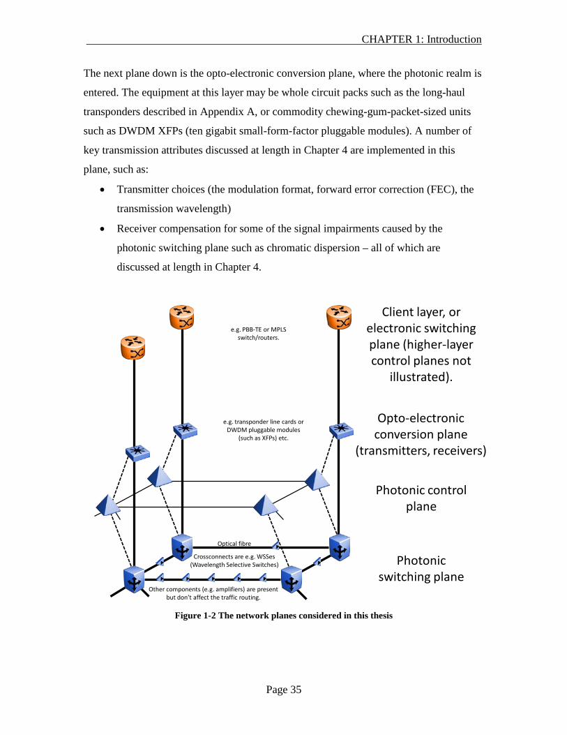
1.6 Network planes diagram
In this section is Figure 1-2, a generic model of the functions within the network explored
within this thesis. It is provided such that later sections in this chapter can be given in the
context of a particular area of this diagram.
The top plane shows a client layer that is connected together via the photonic switching
plane. There will be a quantity of traffic (which may be zero) to be moved between any
pair of its nodes at any time. Some traffic will be broadcast/multicast. The subject matter
of this thesis is the photonic layer, so the nature of the client layer is out of scope of this
thesis except with respect to these traffic demands. As discussed in section 1.5.8, to avoid
bandwidth stranding the client layer will usually be some sort of electronic
switching/multiplexing layer, but photonic techniques to bridge the demand/wavelength
size gap are discussed in section 1.7.
CHAPTER 1: Introduction
Page 35
The next plane down is the opto-electronic conversion plane, where the photonic realm is
entered. The equipment at this layer may be whole circuit packs such as the long-haul
transponders described in Appendix A, or commodity chewing-gum-packet-sized units
such as DWDM XFPs (ten gigabit small-form-factor pluggable modules). A number of
key transmission attributes discussed at length in Chapter 4 are implemented in this
plane, such as:
• Transmitter choices (the modulation format, forward error correction (FEC), the
transmission wavelength)
• Receiver compensation for some of the signal impairments caused by the
photonic switching plane such as chromatic dispersion – all of which are
discussed at length in Chapter 4.
e.g. PBB-TE or MPLS switch/routers.
Photonic switching plane
Opto-electronic conversion plane
(transmitters, receivers)
Client layer, or electronic switching plane (higher-layer control planes not
illustrated).
Photonic control plane
e.g. transponder line cards or DWDM pluggable modules
(such as XFPs) etc.
Crossconnects are e.g. WSSes(Wavelength Selective Switches)
Other components (e.g. amplifiers) are present but don’t affect the traffic routing.
Optical fibre
Figure 1-2 The network planes considered in this thesis

CHAPTER 1: Introduction
Page 36
The next plane down for user data (which does not pass into the control plane) is the
photonic switching plane. This directs the optical signals emitted by the opto-electronic
plane’s transmitters to their corresponding receivers via fibre and switching elements
such as wavelength-selective switches (WSSes). For the purposes of Chapters 2 and 3
this signal-routing function is the primary area of interest. There can be many other
components within the photonic switching plane to help improve the quality of the signal
ultimately received, such as optical amplifiers. Chapter 4 discusses at length the impact
of fibre transmission and optical components upon signal quality, and how to determine
whether the received signal will achieve an acceptable BER as defined in section 1.5.5.
To the side of the diagram between the opto-electronic conversion and photonic
switching planes, forming a parallel layer, is the photonic control plane. Client data does
not flow to this layer, which is why it is illustrated to the side of the data-path. Its key
functions discussed throughout this thesis are to set the photonic switching plane to
implement its route decisions for a wavelength-path, and to configure the transmitter’s
wavelength such that it is not being used along the path of that wavelength-path. Chapter
4 also discusses value that may be derived from adjusting other transmitter parameters
such as modulation format. See section 1.8 for further discussion of the usage of control
planes within this thesis. The control plane will need communication paths to signal to
the hardware it is controlling, and if it is distributed, within its own nodes. The latency of
these communication paths is a significant issue discussed in Chapter 3.
Higher layers have control planes, but these are outside of the photonic scope of this
thesis. Design of a multi-layer control plane including the photonic layer would need to
include all of the factors discussed in this thesis. However, the routing algorithms would
need to be enhanced to be multi-layer. This is an item in Chapter 5’s further work section.
Power balancing (not illustrated) is the function of adjusting network component settings
such that all wavelength-paths are received at a power level that achieves an acceptable
BER (if this is possible). Power balancing is sometimes considered part of the function of
a photonic control plane. However, because it is an independent process from the routing

CHAPTER 1: Introduction
Page 37
and wavelength allocation that is the primary subject of this thesis, it is not further
considered – it is assumed that it will happen automatically in the background. This
assumption reflects the behaviour of the Ciena system described in Appendix A.
1.7 Bridging the gap between wavelength and demand sizes
A problem with WRONs (see section 1.3) is that the total demand from the access layer
will probably not correspond to an integer number of wavelengths. This section reviews
the most common approaches in the literature for addressing this mismatch in the
photonic domain (optical packet switching/optical burst switching), and why they are not
usable at this time. Then the approaches discussed in the remainder of the thesis are
described: a generalised view of the present mode of operation (named here as A-
WRONs, agile WRONs), as well as introducing a less well-known alternative approach
(wavelength path sharing).
1.7.1 Optical packet switching (OPS)
An optical packet switching node inspects a header on each packet that is received and
from this determines on which port to send it to the next node, in similar fashion to an IP
router or Ethernet switch (described in [Boudriga 08]). Thus, the packet makes its way
hop-by-hop to its destination. However, the packet has travelled optically all the way
from source to destination because all intermediate components process the data as light
rather than electrons, thus the disadvantages of OEO conversion are not incurred.
Therefore, the efficiency of IP-style statistical multiplexing can be achieved while
eliminating the expense/power/heat of any electronic switching from the network core,
except for the lesser expense/power/heat of electronic packet header inspection and
routing.
However, because the packets do not arrive according to a pre-coordinated schedule,
there will sometimes be contention for an output port. To avoid packet loss, buffering
must be available. Unfortunately the only known methods of optical buffering are not
very practical (reviewed in [Zhou 03][Bawab 02][Burmeister 08]): e.g. fibre delay lines

CHAPTER 1: Introduction
Page 38
(FDLs) are physically bulky as discussed in [Boudriga 08] and [Mack 08] and as per the
example2
Further, to achieve comparable efficiency of link fill to electronic switches, OPS requires
full wavelength conversion – the ability to wavelength-convert all of the packets
simultaneously arriving on all of their ports at all wavelengths to a different wavelength
than the one they arrived on – to avoid conflicts where the same wavelength from two
; micro-ring resonators allow loops to be embedded on a semiconductor die as
per [Ding 08], although this does not reduce the need for the sheer volume of storage.
Photonic crystals solve the underlying problem by slowing down the light (e.g. as per the
preliminary work in [Baba 07], however, as [Burmeister 08] demonstrates convincingly,
slow-light devices currently suffer from dispersion, bandwidth and loss issues that
prevent them achieving useful amounts of buffering. Burmeister concludes that
recirculating silica or silicon delay lines (which can be integrated onto a silicon wafer)
are a convenient and practical solution. However, taking the benchmark from the
previous footnote of 100ms, using Burmeister’s density figure of 0.1ns/cm, this would
require a cumulative total of 10,000km of delay line. Even his CRS-ideal slow-light
technology achieving 30ns/cm would require approximately 33km of delay line – still
quite impractical.
2 To give an example of the impracticality of the physical bulk of the fibre delay line required to replace the
electronic buffering in a modern Ethernet switch: the Cisco 7600 ES+ series of line cards claims 100ms
buffering/direction per port [Cisco7600ES+]. Taking an example of Corning SMF-28e optical fibre, 100ms
requires a length of N
ct ×(where t = 100ms, c = speed of light, N = refractive index at 1550nm , which is
approx 1.47 [Corning SMF-28e]) approx 20400km , which assuming a single layer of fibre on the
recommended 50mm-diameter spool and an average of the specified 245um coated fibre diameter would
require a spool 31.8km high, which would be infeasibly physically large, without even considering other
issues such as the transmission loss and signal degradation of such a lot of fibre. A practical
implementation would probably need multiple short loops to allow data to be tapped off after less than the
full delay where there was a slot free on the output transmission fibre, but the sum of the lengths of the
short loops would have to at least equal the length calculated above – sending the data around a shorter
loop multiple times would work in the style of a recirculating loop (such as described in Fig 2 of [Boudriga
08]), but would require additional loops for data subsequently received.

CHAPTER 1: Introduction
Page 39
different ports needs to end up on the same egress port [Mohamadzadeh 06]. As yet,
these have not become cheaper than electronic options (as noted in [Zalesky 09]),
although research progresses with e.g. [Raz 09], [Marconi 09].
Therefore, until a breakthrough in the areas of buffering and wavelength conversion
occurs, optical packet switching is generally accepted to be non-commercial, and thus not
further discussed.
1.7.2 Optical burst switching (OBS)
[Qiao 99] introduced optical burst switching as an evolution of optical packet switching
(for more recent reviews, see e.g. [Zalesky 09], [Hernandez 09], [Yoo 06]). The
difference is most clear in the ‘tell and wait’ case, where transmission of a packet is
delayed for a while to allow the header time to be processed by intermediate switching
nodes. This delay means that further packets to the same destination may have arrived
before the first can be transmitted, such that a stream of packets may be transmitted
together as a burst. One aspect of further work has been on burst release strategies: when
to deliberately delay the signalling of a burst to increase its size and thereby gain
efficiency, e.g. [Zalesky 08].
Figure 1-3 shows a generic diagram of optical burst switching, where a photonic-
switched core (‘Optical layer’) is terminated by electronic routers (i.e. with electronic
buffering capability) which aggregate up packet flows into bursts across the photonic
core.
[Qiao 99] discussed the use of fibre delay lines. Some more recent papers share this idea
such as [Boudriga 08]. For the reasons discussed in the OPS section, this thesis will
ignore this aspect of Qiao’s proposal as currently impractical and use the now
commonly-held definition of OBS as including no optical buffering as per
[Weichenberg 06], [Weichenberg 07] and [Zalesky 08].

CHAPTER 1: Introduction
Page 40
Figure 1-3 Generic optical burst switching (OBS) network diagram, after [Duser 02]
Because core congestion is inevitable where the burst is transmitted without knowledge
that there is capacity for it to traverse the network (as Qiao proposed), and this leads to
burst loss, inefficient routing (via deflection routing) or a need for buffering, an
alternative scheme has been proposed where a signalled acknowledgement that
bandwidth is available is required before a transmitter will send a burst. In essence, a
short-lived connection is established for the burst. This scheme was proposed as
Wavelength Routed Optical Burst Switching (WROBS) in [Duser 02] or Optical Flow
Switching in [Weichenberg 06]. This thesis will refer to it as WROBS.
As a WROBS scheme must buffer up any traffic that arrives between the decision that a
burst should be sent and the time that the burst is authorised, WROBS bursts are longer
than unacknowledged bursts (tens of kilobytes [Duser 02]) for the same burst-sending
strategy. To justify the signalling overhead of setting up a tell-and-wait burst, it is usual
for the burst-sending strategy to wait from the arrival of the first packet of a burst for as
long as its latency budget will allow, to maximise the opportunity for more packets to
arrive that can join that burst.
Photonic layer
Burst aggregation
layer
Electronic burst aggregator (router/switch)
Photonic burst switch
CHAPTER 1: Introduction
Page 41
More recent work has covered Quality of Service (QoS) in OBS. E.g. reserved sub-
wavelength bandwidth connections over an OBS network reviewed in e.g. [Hernandez
09], as is the possibility of sharing such links with best effort traffic; [Boudriga 08]
discusses using buffering to achieve sophisticated QoS like Ethernet or IP; while [Das
08] shows convincingly that adjusting the average burst size according to the congestion
level will increase throughput.
To minimise dropping (or buffering) on congestion for tell-and-go, [Qiao 99] proposed
using deflection routing – the idea of sending the burst out of an alternative port where
there might be available capacity to get it to its destination. That is to say, the burst is
deliberately sent the ‘wrong’ way as the only alternative is dropping it.
As with OPS, reasonable efficiency is only achieved in tell-and-go type schemes if full
wavelength conversion is available. For the reasons discussed in the OPS section, this
will be regarded as impractical until a breakthrough is made in the field and disregarded
for the purposes of this thesis.
Suitability of these approaches is split by network size and target traffic QoS.
Acknowledged bursts have the advantage that the data will not be lost in transit and so
provide predictable performance characteristics, as opposed to unacknowledged bursts
which may require retransmission of the user data. However, unacknowledged burst
systems do not need to wait for a round-trip delay before transmitting, offering lower
minimum/expected latency and being able to work networks three times as large for a
given tolerable latency (because this must be divided between the signalling round-trip
and the transmission time in WROBS).
Therefore, lacking buffering/wavelength conversion as per OPS, OBS is not an option for
the general case of large national networks. [Duser 02] calculates that if an edge delay
constraint of 10ms (very generous when low latency is now a key differentiator in the
industry) is acceptable then a network diameter of 1500km may be achieved – inadequate
for US and other larger continental networks. Further, fast switching components are
CHAPTER 1: Introduction
Page 42
required for large-scale networks/networks at high utilisation – for small-scale OBS
networks many wavelength routes can be pre-set with the chosen transmitter wavelength
selecting which one will get its traffic to its destination, but this strands capacity and thus
is not scalable.
1.7.3 Agile wavelength-routed optical networks (A-WRONs)
In this thesis, agile wavelength-routed optical networks (A-WRONs) are defined as
being WRONs, where wavelengths are re-arranged/added according to a planning cycle
(which may be triggered by a link fill threshold being exceeded) rather than immediately
in reaction to a particular packet arrival. Spare capacity is provisioned with a goal that
new requests for bandwidth received until the next opportunity to add wavelengths will
not be blocked due to capacity exhaustion.
With longer planning cycle frequencies (hours/days), A-WRONs correspond to the state
of the commercial art (see Appendix A) of ROADM (reconfigurable optical add-drop
multiplexer)-based line systems, although a human is usually involved in interpreting
demands and considering network re-engineering.
Replace that human with an automated function, and in the limit of extremely fast
planning cycles this becomes very similar to WROBS, but critically it is still different in
that OBS is trying to serve a packet that has just arrived, whereas A-WRON is trying to
serve the unknown packets that are about to arrive.
As the planning cycle becomes faster (more agile), less spare capacity bandwidth is
required, so theoretically the network should operate more efficiently. Assessing the
actual achievable value of this agility is the subject of Chapter 3, which also more
thoroughly defines A-WRONs.
The same concept is described as Optical Circuit Switching (OCS) by [Zalesky 09],
however his analysis is limited to an extremely fast (millisecond ‘planning interval’)
version. Further Zalesky’s connections are bidirectional, for no apparent reason except

CHAPTER 1: Introduction
Page 43
convention in connection setup. This thesis assumes unidirectional wavelength-paths, as
an upper bound of efficiency (as bidirectional connections are just a special case of
unidirectional connections). This assumption is not fully realistic as many applications
require approximately symmetric latency, which may be achieved by a routing constraint
to this effect, but is usually and more simply addressed by routing bidirectional
wavelengths.
1.7.4 Wavelength path sharing (WPS)
A-WRONs provide a dedicated wavelength for each wavelength demand. They will
therefore suffer from bandwidth stranding. WPS (proposed in [Myers 01] addresses this
by allowing a network with slow wavelength-switching times (unlike OBS/OPS) to still
achieve sub-wavelength granularity at the optical layer.
8
10
6
2
3
1
4
5
7
9
11
0
13
12Path 1
Path 2
Key
n
This logical path transits this node transparently. [Passive node]This logical path transits this node with add/drop capability. [Active WPS node]
Node with identifier ‘n’.
Fibre
Figure 1-4 Basic principles of WPS illustrated on the NSFNet (see Appendix B)
It does this by allowing multiple demands to share a single wavelength without requiring
the photonic switch matrix to cross-connect at the speed of demand variation.

CHAPTER 1: Introduction
Page 44
Figure 1-4 shows the principle of WPS, where a wavelength-path (Path 1) is established
along a route 2-1-8-9. This path can serve demands between any of the nodes that are
active along the path - 2, 8 and 9. Node 1 is acting as a conventional WRON switched
node.
Similarly, path 2 is a wavelength-path along the route 2-4-5-7-8-9-13. Nodes 2, 5 and 13
are active, with 4, 7, 8 and 9 being passive. This second path is shown to make the point
that a node may be active for one path, but passive in another – nodes 8 and 9 in this
figure. A passive node requires less equipment and introduces less optical impairment
into the path.
Chapter 2 introduces WPS in more depth and proposes a number of enhancements.
1.8 Photonic control planes, routing and path computation
elements (PCEs)
Each of the previous sub-sections (A-WRONs and WPS) has assumed the ability to set
up and tear down wavelength-paths along (near-)optimal routes. How optimal those
routes are determines the efficiency of the network – how much traffic it can carry before
money must be spent on addition of capacity. To put that another way, for a network
operator, the routing efficiency determines how much revenue-earning traffic they can
support with their principal capital asset, the network. Thus, effective routing is a key
factor in their continued commercial survival, and therefore extremely important.
In the context of this thesis, the “Photonic control plane” is defined as a software entity:
- Of which a user can request connectivity;
- That can create and delete wavelength-paths by commanding nodes to set up
sections of that path (such as nodal cross-connections) in response to traffic
demands that may be sub-wavelength.

CHAPTER 1: Introduction
Page 45
This is very similar to a non-photonic control plane, except that this entity is serving its
demands with wavelength paths. Implicit within that are photonic-specific constraints
such as wavelength continuity and viability as discussed elsewhere in this chapter.
This definition includes technologies commonly described as control planes such as the
ASTN/ASON [ASTN] architecture and [GMPLS] protocols/architecture. However, it
deliberately also includes management systems that directly control nodes for the purpose
of path setup. This inclusion is made because the routing function is the same for both
cases, so this thesis does not make a distinction. Some example differences – not relevant
to this thesis – are that:
• Signalled control planes usually: reside on the controlled equipment; form a
highly-distributed computing environment (usually one instance per node); react
to network events such as faults (in addition to external stimuli such as new
connection requests that management systems also react to); may provide some
form of restoration/protection on failure.
• Management systems usually: reside on a server rather than the controlled
equipment; form a highly-centralised computing environment (the basic
configuration being one or a resilient pair of servers); only provision the network
when directed by external stimuli (like new connection requests); may provision
(but not directly provide) protection mechanisms in the network.
There are exceptions to each of the differences listed – for example, the Nortel LH1600
OPC card was a management system that ran on an HP workstation that was physically
housed in a card that sat in an optical transmission shelf and managed the local sub-
network.
However, the control/management plane distinction provided above does not cover all
possibilities as it is legitimate, and within e.g. the [GMPLS] standard, for a higher-level
entity (e.g. a management system or OSS) to fully-specify (every port, every node) all
routes explicitly, meaning that the actual control plane would be offering no intelligence
to the question of where traffic is placed.
CHAPTER 1: Introduction
Page 46
Therefore, define:
“Control plane routing”: the algorithms that determine which wavelength-paths should
be establish to serve a given set of wavelength-sized and sub-wavelength demands, and
which wavelength-links each wavelength-path should be routed over.
Then, if a higher-level OSS is indeed doing all of the routing calculations, it is considered
part of the control plane routing.
This is a broader definition than classic routing and wavelength allocation (RWA – e.g.
used in [Raza 08], [Duser 02]) as the input of control plane routing is not a set of
wavelength demands, but a set of sub-wavelength demands. Further, as will be seen later,
a key parameter investigated is how fast the wavelengths are re-arranged to suit the sub-
wavelength demands.
The concept of ‘outsourcing’ the routing function from control planes to a separate entity
was introduced in [RFC4655] as a Path Computation Element (PCE). This is a more
limited definition than the one in this chapter because it assumes there is a GMPLS
control plane in existence to receive the original connection request, rather than allowing
that to be a management system. Further, the stated purpose of the Internet Engineering
Task Force’s (IETF’s) PCE work is to define a mechanism to allow the separation of the
PCE – deemed a hard problem that may need to be handled differently for each
operator/domain – from the standard signalling. The IETF PCE Working Group does not
actually attempt to solve the routing problem. PCE is sometime informally used with a
more general definition similar to “control plane routing”, but the term “PCE” has a
specific and well-defined meaning in the IETF and so the separate term “control plane
routing” is defined for use in this thesis for the general case.
In summary, the control plane usage within this thesis is compatible with but does not
assume GMPLS or ASTN. This thesis is focussed exclusively on the routing question and
is not concerned about any other aspect of control planes, for example the choice of
method of signalling information between nodes.
CHAPTER 1: Introduction
Page 47
1.9 Research question and current open issues
This thesis addresses the research question of how the control plane routing should
address changing traffic demands.
To investigate this, the following significant issues must be addressed:
1. WPS must be evaluated as an alternative to fast switching in A-WRONs. The
integer linear programming (ILP)-based routing algorithm given with its original
proposal in [Myers 01] must be evaluated for speed of execution, and thus
practicality for on-line use. A faster alternative routing algorithm must be
proposed, and evaluated for optimality against the ILP and theoretical lower
bounds.
2. The value of agility in A-WRONs must be assessed. First, a formal definition of
agility must be provided. Many switching technologies are available to offer
different network agilities, however the benefit to the network operator of
faster switching/greater agility must be evaluated in terms of the greater
network efficiency that the control plane can achieve.
3. Network engineering approaches such that the control plane routing can
deliver optically viable wavelength-paths must be reviewed, the most optimal
approach proposed and evaluated for practical applicability. This must be done
for both traditional (on-off keyed) and newer modulation formats/detection
techniques.
1.10 Thesis structure
In order to address these issues, the remainder of this thesis is structured as follows:
In Chapter 2, WPS is presented in detail. The Integer Linear Programming (ILP)
formulation given by Myers to find routes, while providing optimal results, is shown to
be unacceptably slow for online execution, so a new heuristic algorithm is provided.
Performance of the two is then compared. A new ILP formulation for allocation of
specific wavelengths, obeying the wavelength continuity constraint, is provided. The

CHAPTER 1: Introduction
Page 48
best-known heuristic for WRONs, AUR-E is adapted for WPS and compared with the
Myers ILP.
In Chapter 3, the value of network agility is evaluated. Firstly, a formal definition of
agility is provided for switches, wavelength-paths and networks, with the relationship
between these and other factors that may contribute to them. The literature on switching
speeds is reviewed to extract the range of switching speeds currently available. Then,
new simulations are performed that evaluate the practical benefit achieved by
reconfiguring the network at different intervals, in terms of delaying the time at which an
upgrade must be performed, i.e. new investment must be applied to the network.
In Chapter 4, optical viability is reviewed. Causes of non-viability are discussed. Use of
viability in a control plane context is described. Network engineering approaches that
avoid the need to actively calculate viability for each new wavelength are reviewed.
Techniques to incorporate optical viability into routing algorithms are reviewed. Error
analysis is used to show that open-loop calculation based on previously-measured link
characteristics, when using the best commercially available measurement equipment, is
no better than performing predictions based on equipment specifications. The differences
in impairment calculations for phase-modulated coherent systems are considered, and
adaptation of the specify-and-predict approach to coherent viability calculation is
described.
In Chapter 5 conclusions and ideas for further work are presented.
1.11 Contribution of this work
The novel contributions of this thesis are the following:
i) An alternative hardware configuration for WPS that delivers savings in OE/EO
conversions (the amount varying with acceptable blocking probability and traffic
load), where the one originally proposed in [Myers 01] did not.
CHAPTER 1: Introduction
Page 49
ii) A heuristic algorithm for routing WPS logical connections to achieve execution
time savings relative to Myers’ ILP, at some cost in efficiency of the result. This
was published in [Friskney 03].
iii) An ILP formulation for optimal wavelength allocation. This was included in
[Friskney 03].
iv) A heuristic algorithm for simultaneous routing and wavelength allocation for
WPS, derived from AUR-F and AUR-E, reducing the efficiency cost relative to
Myers’ ILP.
v) A definition of network agility.
vi) A categorisation of switch times by application type.
vii) Simulations to quantify the effects in terms of network bandwidth efficiency of
increased network agility on an infrastructure wavelengths system.
viii) A comparison of methods of optical viability calculation. A shorter version was
co-published as [Peeters 04]. The author collaborated on a related technique, co-
filed and granted as US patent [Peeters 03], which is not otherwise discussed in
this thesis.
ix) Error analysis for a measure-and-predict optical viability. Published in
[Friskney 02].
x) The proposal of the adaptive use of phase/amplitude modulation to achieve
optimal spectral efficiency for a given set of bitrates and reach requirements.
Granted as US patent [Friskney 02c].

CHAPTER 1: Introduction
Page 50
1.12 Publications arising in the course of the research described in this thesis
[Dong 03] S. Dong, C. Phillips, R. Friskney, "Differentiated-Resilience Provisioning in
Wavelength-Routed Optical Networks". International Teletraffic Congress (31st August-
5th September 2003) 2003, Berlin, Vol. 5A-B, pp921-930.
[Friskney 02] R. Friskney, K. Warbrick, S. Poliakoff, R. Heath, "Link-based photonic
path performance prediction and control". Proc. European Conference on Optical
Communications (ECOC) 2002 (6th-12th September 2002), Copenhagen, Vol. 3, pp1-2.
Paper 7.4.3.
[Friskney 03] R. Friskney, "Path allocation for wavelength path sharing". Proc. London
Communications Symposium (LCS) 2003 (8th-9th September 2003).
[Peeters 04] B. Peeters, D. Forbes, R. Friskney, J. Shields, "Optimal routing in hybrid
networks by decoupling the route calculation from the assessment of optical route
viability". European Conference on Networks & Optical Communications (NOC) 2004
(29th June-1st July 2004), Eindhoven.
[Lao 04] R.N. Lao, R. Friskney, R.I.Killey, "Effect of Sparse Wavelength-Conversion
on Network Tolerance to Inaccuracy in Traffic Load Forecasts". European Conference on
Optical Communication (ECOC) 2004 (September 2004), Stockholm.
[Lao 04-2] R.N. Lao, R. Friskney, R.I.Killey, "Investigation of the tolerance of
wavelength-routed optical networks to inaccuracy in traffic load forecasts". Optical Fiber
Communication Conference (OFC) 2005 (6th-11th March 2005), Vol. 4. Paper: OThS4.
[Lao 05] R. N. Lao, R. Friskney, R. I. Killey, "Investigation of the tolerance of
wavelength-routed optical networks to inaccuracy in traffic load forecasts". Journal of
Optical Networking, Vol. 4, Issue 3 (3rd
http://www.osa-jon.org/abstract.cfm?URI=JON-4-3-144
March 2005), pp144-156.

CHAPTER 1: Introduction
Page 51
[Dong 06] S. Dong, C. Phillips, R. Friskney, "Differentiated-Resilience Provisioning for
the Wavelength-Routed Optical Network". Journal of Lightwave Technology, Vol. 24,
Issue 2 (February 2006), pp667-673.
1.12.1 Patents pending and granted
The following patents which I contributed to were filed by Nortel. They were subjected
to an internal peer review before doing so to determine whether it is worth the
considerable cost in attorney fees etc. to have them professionally drafted and filed, and
in which countries it was deemed strategic to do so. Grant occurs only after an extensive
multi-year government examination, with iterative legal and technical argument and re-
drafting, which is why grant occurs many years after filing. Note: The title submitted is
often changed by the attorneys in each country and therefore the one listed here may not
correspond to official records, hence reference numbers are provided where known.
[Fisher 02] D. Fisher, N. Bragg, R. Friskney, “Concatenated Transmission of
Synchronous Data”. US filing 10/054,188, filed June 2002. Granted 22nd April 2008 as
US patent 7,362,777.
[Friskney 02a] R.Friskney, R. Heath, K. Cordina, “Transient Location for Optical
Networks”. US filing 10/109,199, filed March 2002.
[Friskney 02b] R. Friskney, A. Robinson, R. Spagnoletti, “Optical Communications
System”. US filing 10/185,097, filed June 2002.
[Friskney 02c] R. Friskney, A. Sparks, R. Spagnoletti, Robin Rickard, “Optical
Communications System”, US filing 10/180,595, filed June 2002. Granted 30th December
2008 as US Patent 7,471,903.
CHAPTER 1: Introduction
Page 52
[Parry 02] S. Parry, A. Sparks, R. Friskney, R. Spagnoletti, D. Watley, “Method and
system for locating faults in an optical network”. US filing 10/298,098, filed November
2002.
[Friskney 02d] R. Friskney, A. Sparks, S. Parry, N. Davis, “Determining and using value
of traffic relying on a given component of a communications network”. US filing
10/261,069, filed September 2002. Granted in UK as patent number 2,393,606 21st
December 2005. Granted 15th July 2008 as US Patent 7,400,583.
[Friskney 02e] R. Friskney, S. Dong, C. Phillips, “Differentiated Resilience in Optical
Networks”. US filing 10/323,409, filed 18th December 2002.
[Shields 03] J. Shields, R. Friskney, “Optical Routing and Service Activation”. US filing
10/656,544 5th September 2003.
[Friskney 03a] R. Friskney, N. Baker, F. Davis, S. Dong, C. Phillips, “Methods and
apparatus for determining a path in a communications network”. US filing 10/675,760,
filed September 2003.
[Peeters 03] B. Peeters, R. Friskney, J. Shields, “Method of and system for routing in a
photonic network”. US filing 10/656,543, filed September 2003. Granted 13th January
2009 as US Patent 7,477,843.
[Friskney 04] R. Friskney, N. Bragg, S. Parry, P. Ashwood-Smith, D. Allan, S.
Brueckheimer, “Direct configuration of ethernet switch bridging tables for the
establishment of virtual circuits for traffic management”. US filing 10/818,685, filed
April 2004, also US filing 12/196909 filed 22nd August 2008, also US filing 10/593108
filed 21st May 2007. WO filing 2005099183. European filing EP1735961 (A0, A1),
Canada CA2560702. Granted in UK 28th March 2007 as patent GB 2,422,508 and 5th
December 2007 as GB 2,438,767. This is the fundamental patent first proposing the
technology in IEEE standard 802.1Qay.
CHAPTER 1: Introduction
Page 53
[Parry 05] S. Parry, R. Friskney, “Improved Multilink Trunking for Provider Backbone
Bridges”. US filing 11/264634 filed 1st November 2005. Granted 13th April 2010 as US
Patent 7,697,528. European filing 16th July 2008 EP1943785.
[Bragg 06] N. Bragg, P. Bottorff, D. Allan, R. Friskney, S. Parry, “Planning routes and
allocating identifiers to routes in a managed frame-forwarding network”. US filing
11/343996 filed 31st January 2006. Granted 13th July 2010 as US Patent 7,756,035. Filed
in Europe 29th October 2008 as EP1985072. Also US filing 12/752228 filed 1st April
2010.
[Allan 06] D. Allan, N. Bragg, M. Holness , R. Friskney, S. Parry, “Provider backbone
bridging – provider backbone transport internetworking”. US filing 11/479694 filed 30th
June 2006. Filed in Europe 16th July 2008 as EP1943783.
[Friskney 07] R. Friskney, S. Parry, D. Allan, N. Bragg, “Scaling OAM for point-to-
point trunking”. US filing 11/845930, 28th August 2007.
[Friskney 07] R. Friskney, C. Ramsden, “Reducing configuration required in
802.1ag/Y.1731 OAM signalling”. US filing 11/964534 filed 25th December 2007.
[Bragg 07] N. Bragg, D. Allan, S. Parry, R. Friskney, S. Brueckheimer, “An improved
method for network evolution”. US filing 11/962476 filed 21st
US versions of filings may be seen at http://www.uspto.gov by using the filing numbers
given. European and some other filings can be found at http://www.ipo.gov.uk/ or more
readily http://gb.espacenet.com/.
December 2007. Also
filed as KR20100114025, EP2232781, CN101926129, WO2009079771.

CHAPTER 1: Introduction
Page 54
1.13 Chapter references
[ASTN] ITU G.8081, G.807, G.8080, G.7713 et al. Currently summarized as
http://www.itu.int/ITU-T/2001-2004/com15/otn/astn-control.html.
[Baba 07] T. Baba, “Toward Photonic Crystal Optical Buffer”. Proc. IEEE LEOS Lasers
and Electro-Optics & Quantum Electronics and Laser Science, Vols 1-9 (2008), page
1844.
[Bagula 07] A. Bagula, “On Achieving Bandwidth-Aware LSP/λSP
Multiplexing/Separation in Multi-layer Networks”. IEEE Journal in Selected Areas in
Communications, Vol. 25, No. 5 (June 2007), pp 987-1000.
[Baroni 98] Stefano Baroni, “Routing and wavelength allocation in WDM optical
networks”. University College London PhD thesis. May 1998.
[Bawab 02] T. El-Bawab, J-D. Shin, “Optical packet switching in core networks: between
vision and reality”. IEEE Communications Magazine, Vol. 40, Issue 9 (Sept 2002), pp60-
65.
[Boudriga 08] N. Boudriga, A. Lazzez, Y. Khlifi, M. Zghal, “All Optical Network
Switching: A New Scheme for QoS Provision and Virtual Memory Control”.
International Conference on Transport Optical Networks 2008 (June 2008), pp 178-182.
[Brehon 07] Y. Brehon, D. Kofman, M. Pioro, M. Diallo, “Optimal Virtual Topology
Design using Bus-Label Switched Paths”. IEEE Journal on Selected Areas in
Communications, Vol. 25, No. 5 (June 2007), pp1001-1010.
[Breuer 03] D. Breuer, H-J. Tessmann, A. Gladisch, H. Foisel, G. Neumann, H. Reiner,
H. Cremer, “Measurements of PMD in the installed fiber plant of Deutsche Telekom”.
LEOS Summer Topical Meetings 2003, Holey Fibers and Photonic Crystals/Polarization

CHAPTER 1: Introduction
Page 55
Mode Dispersion/Photonics Time/Frequency Measurement and Control, 14th-16th
[Cisco 11] “Cisco Visual Networking Index – Forecast and Methodology, 2010-2015”,
June 1, 2011.
July
2003, MB2.1/5.
[Burmeister 08] E. Burmeister, D. Blumenthal, J. Bowers, “A comparison of optical
buffering technologies”. Optical Switching and Networking, Vol. 5, No. 1 (March 2008),
pp10-18.
http://www.cisco.com/en/US/solutions/collateral/ns341/ns525/ns537/ns705/ns827/white_
paper_c11-481360_ns827_Networking_Solutions_White_Paper.html
[Das 08] A. Das, P. Banerjee, A. Das, “Performance evolution in Optical Burst Switched
Networks”. Proc. IFIP International Conference on Wireless and Optical
Communications Networks 2008 (5th-7th
[Deloitte 07] Deloitte, “Telecommunications Predictions: Technology Media &
Telecommunications Trends 2007”.
May 2008), pp1-5.
http://www.deloitte.com/dtt/cda/doc/content/dtt_TelecomPredictions011107.pdf
[Ding 08] Y. Ding, X. Zhang, X. Zhang, D. Huang, “Proposal for loadable and erasable
optical memory unit based on dual active microring optical integrators”. Optics
Communications, Vol. 281, Issues 21 (November 2008), pp 5315-5321.
[Duser 02] M. Duser, P. Bayvel, “Analysis of a dynamically wavelength-routed optical
burst switched network architecture”. Journal of Lightwave Technology, Vol. 20, No. 4
(April 2002), pp574-585.
[Duser 05] M. Duser, “Investigation of the impact of traffic growth and variability on
future network architectures”. Proc. European Conference on Optical Communications
2005 (25th-29th September 2005), Vol. 5, pp27-30. Paper Tu 4.1.2.
CHAPTER 1: Introduction
Page 56
[Falcao 02] P. Falcao, E. Mannie-Corbisier, M. Moelants, P. Noel, “Deployment of next
generation WDM networks in Europe“. Proc. Optical Fibre Communication Conference
(OFC) 2002 (17th-22nd March 2002), pp45-46. Paper TuH4.
[GMPLS] IETF RFC3471 L. Berger (Editor), “Generalized Multi-Protocol Label
Switching (GMPLS) Signaling Functional Description”. January 2003.
[Gong 08] S. Gong, B. Jabbari, “Optimal and efficient end-to-end path computation in
multi-layer networks”. IEEE International Conference on Communications 2008 (19th-
23rd
[Hillerkuss 11] D. Hillerkuss et al., “26 Tbit s
May 2008), pp5767-5771.
[Goralski 00] W. Goralski, “SONET”, McGraw-Hill. Second edition. Page 557.
[GR-253-Core] Telcordia, “Synchronous Optical Network (SONET) Transport Systems:
Common Generic Criteria”. GR-253-Core, Issue 4 (December 2005), page 4-5 “Optical
Parameter Definitions and Interface Requirements”.
[Hernandez 09] J. Hernandez, J. Aracil, V. Lopez, J. Garcia-Dorado, L. de Pedro,
“Performance analysis of asynchronous best-effort traffic coexisting with TDM
reservations in polymorphous OBS networks”. Photonic Network Communications, Vol.
17, Issue 2 (April 2009), pp 93-103.
−1 line-rate super-channel transmission
utilizing all-optical fast Fourier transform processing”. Nature Photonics advanced online
publication 22nd May 2011 “doi:10.1038/nphoton.2011.74”.
http://dx.doi.org/10.1038/nphoton.2011.74.
[IEEE 802.3-2005] IEEE Computer Society, “802.3: Carrier sense multiple access with
collision detection (CSMA/CD) access method and physical layer specifications”. 802.3-
CHAPTER 1: Introduction
Page 57
2005. For example 1000Base-X is in Part 3, page 33: “Physical Coding Sublayer (PCS)
and Physical Medium Attachment (PMA) sublayer, type 1000Base-X”.
[IEEE 802.3ba] IEEE P802.3ba 40Gbps and 100Gbps Ethernet Task Force
[Kohn 06] M. Kohn, “A new efficient online-optimization approach for SDH/SONET-
WDM multi-layer networks”. Proc. Optical Fiber Communication Conference (OFC)
2006 (5th-10th March 2006). Paper OFG8.
[Mack 08] J.P. Mack, E.F. Burmeister, H.N. Poulsen, J.E. Bowers, D.J. Blumenthal,
“Synchronously Loaded Optical Packet Buffer”. IEEE Photonics Technology Letters,
Vol. 20, No. 21 (November 2008), pp1757-1759.
[Majumder 05] S.P. Majumder, S.M.R. Kabir, R. Rahman, F. Imtiaz, M. Moniruzzaman,
“A new architecture of TDM switch”. IEEE Pacific Rim Conference on
Communications, Computers and Signal Processing 2005 (24th-26th August 2005),
pp372-375.
[Malenstein 09] G. van Malenstein, B. Peeters, H. Trompert, “Dynamic lightpaths at
SURFnet: from pilot to production”. Trans-European Research and Education Network
Association (Terena) Network Conference 2009 (8th-11th June 2009).
[Marconi 09] J. Marconi, S. Cerquieri Jr., J. Robinson, N. Sherwood-Droz, Y. Okawachi,
H. Hernandex-Figueroa, M. Lipson, A. Gaeta, H. Fragnito, “Performance investigation of
microphotonic-silicon devices in a field-trial all-optical network”. Optics
Communications, Vol. 282, Issue 5 (1st
[MINTS] Minnesota Interenet Traffic Studies (MINTS).
March 2009), pp849-855.
http://www.dtc.umn.edu/mints/home.php. Regularly updated with internet usage data.

CHAPTER 1: Introduction
Page 58
[Mohamadzadeh 06] H. Mohamadzadeh, M. Sabaei, “A Two Levels Architecture For
Bufferless WDM Optical Packet Switches”. Proc. Information and Communication
Technologies (ICTTA) 2006 (24th-28th
[OIF-FD-100G-DWDM] Optical Internetwork Forum (OIF) Implementation Agreement
OIF-FD-100G-DWDM-01.0 “100G Ultra Long Haul DWDM Framework Document”.
June 2009.
April 2006), Vol. 2, pp2036-2041.
[Myers 01] A. Myers, “Architecture for Optical Burst Switching”, MRes Thesis 2001,
University College London.
[Myers 01a] A. Myers, “Performance of the Just-Enough-Time (JET) scheme for Optical
Burst Switching”. Proc. London Communications Symposium September 2001, pp163-
166.
http://www.oiforum.com/public/documents/OIF-FD-100G-DWDM-01.0.pdf
[Qiao 99] C.M. Qiao, M.S. Yoo, “Optical burst switching (OBS) - a new paradigm for an
optical Internet”. Journal High Speed Networks, vol 8, no 1 (January 1999), pp69-84.
[Raz 09] O. Raz, J. Herrera, H. Dorren, “Enhanced 40 and 80 Gb/s wavelength
conversion using a rectangular shaped optical filter for both red and blue spectral
slicing”. Optics Express Vol. 17, Issue 3 (2nd February 2009), pp1184-1193.
[Richter 11]T. Richter, E. Palushani, C. Schmid-Langhorst, Markus Nölle, R. Ludwig, C.
Schubert, “Single Wavelength Channel 10.2 Tb/s TDM‐Data Capacity using 16‐QAM
and coherent detection”. Proc. Optical Fiber Communication Conference (OFC) 2011,
Postdeadline paper PDPA9.
[RFC4655] A. Farrel, J.-P. Vasseur, J. Ash, “A Path Computation Element (PCE)-Based
Architecture”. Internet Engineering Task-Force (IETF) Request For Comments 4655.
CHAPTER 1: Introduction
Page 59
[Sahara 08] A. Sahara, T. Ono, J. Yamawaku, A. Takada, S. Aisawa, M. Koga,
“Congestion-Controlled Optical Burst Switching Network With Connection Guarantee:
Design and Demonstration”. Journal of Lightwave Technology, Vol. 26, No. 14 (15th July
2008), pp 2075-2008.
[Sivarajan 04] K.N. Sivarajan, “Optical fibre networks and systems in India “. Proc.
Optical Fiber Communications Conference (OFC) 2004 (23rd-27th February 2004), Vol.
1. Paper WH6.
[Swanson 08] B. Swanson, G. Gilder, “Estimating the Exaflood: The impact of Video &
Rich Media on the Internet: A “zettabyte” by 2015?”. January 2008, Discovery Institute.
[Yoo 06] S.J. Ben Yoo, “Optical Packet and Burst Switching Technologies
for the Future Photonic Internet”. Journal of Lightwave Technology, Vol. 24, No. 12
(December 2006), pp 4468-4492.
[Yu 05] S. Yu, W. Gu, “A Tunable Wavelength Conversion and Wavelength Add/Drop
Scheme Based on Cascaded Second-Order Nonlinearity With Double-Pass
Configuration”. IEEE Journal of Quantum Electronics, Vol. 41, No. 7 (July 2005),
pp1007-1012.
[Weichenberg 06] G. Weichenberg, V.W.S Chan, M. Medward, “On the Capacity of
Optical Networks: A Framework for Comparing Different Transport Architectures”.
Proc. IEEE International Conference on Computer Communications April 2006, pp 1-13.
[Weichenberg 07] G. Weichenberg, V.W.S Chan, M. Medward, “On the capacity of
optical networks: A framework for comparing different transport architectures”. IEEE
Journal Selected Areas in Communications, Vol 25, Issue 6 (August 2007), pp 84-101.
CHAPTER 1: Introduction
Page 60
[Zalesky 08] A. Zalesky, H.L. Vu, “Designing an Optimal Scheduler Buffer in OBS
Networks”. Journal of Lightwave Technology, Vol. 26, No. 14 (July 2008), pp 2046-
2054.
[Zalesky 09] A. Zalesky, “To Burst or Circuit Switch?”. IEEE/ACM Transactions on
Networking, Vol. 17, No. 1 (February 2009), pp305-318.
[Zhou 03] P. Zhou, O. Yang, “How practical is optical packet switching in core
networks?”. IEEE Global Telecommunications Conference (Globecom) 2003, Vol. 5,
pp2709-2713.

CHAPTER 2: Wavelength Path Sharing
Page 61
Chapter 2 Wavelength path sharing (WPS) In the previous chapter, it was shown that agile wavelength routed optical networks are
important, and the design challenges for these were discussed – notably in serving sub-
wavelength demands photonically to achieve advantages such as eliminating the cost of
optical-to-electrical (OE) and electrical-to-optical (EO) conversions. In addition, an
approach (wavelength path sharing) was introduced for serving such demands without
using the comparatively fast switching speeds of OPS/OBS (ns/ms, as discussed in
Chapter 1) but while still achieving sub-wavelength granularity.
In this chapter, wavelength path sharing and its advantages as introduced by [Myers 01]
are further described. The shortcomings of this approach are then described, in terms of
the hardware configuration proposed by Myers not delivering savings in OE/EO
conversions relative to a fully-electronic switch. An alternative hardware configuration is
proposed that addresses this shortcoming.
Myers provided an integer linear programming formulation for finding wavelength-path
routes for WPS. This is referred to as M-ILP within this chapter. However, as an ILP
with bounded variables is NP-hard, this will scale poorly in execution time. Indeed,
Myers had to use a restricted formulation to get results on his limited test networks.
Therefore a novel heuristic is proposed for WPS control plane routing – the longest-route
first (LRF) algorithm. The performance of this alternative is then evaluated for
comparison with Myers’s wavelength count results.
A new wavelength allocation ILP formulation (WA-ILP) is then introduced. WA-ILP is
then used in order to re-evaluate the LRF heuristic, under the wavelength-continuity
constraint, versus the M-ILP formulation.
Finally, a further novel heuristic (AUR-F), this time performing simultaneous routing and
wavelength allocation, is also provided (as an extension to an A-WRON version) and
evaluated.

CHAPTER 2: Wavelength Path Sharing
Page 62
2.1 Wavelength path sharing (WPS) principles and advantages
Wavelength path sharing (WPS) is the subject of this chapter. Therefore, this section
provides an outline of WPS as originally defined in [Myers 01]. The next section
describes and compares similar schemes in the literature.
The principle of wavelength path sharing is illustrated in Figure 2-1. In [Baroni 98]’s
usage of WRONs, defined as "A-WRONs" in Chapter 1, a wavelength-path (which
Baroni refers to as a lightpath) is allocated from a source to a destination node via zero or
more intermediate nodes. Critically, the intermediate nodes cannot receive, or
add/remove traffic to/from the wavelength-path.
8
10
6
2
3
1
4
5
7
9
11
0
13
12Path 1
Path 2
Key
n
This logical path transits this node transparently. [Passive node]This logical path transits this node with add/drop capability. [Active WPS node]
Node with identifier ‘n’.
Fibre
Figure 2-1 Basic principles of WPS. Two example paths overlaid on the NSFNet (see Appendix B)
topology. Reproduced from Chapter 1.
By comparison, in WPS, some or all of the intermediate nodes may be ‘active’, defined
as the ability to receive/intercept the traffic or inject their own. Thus, provisioned

CHAPTER 2: Wavelength Path Sharing
Page 63
wavelength routes may be time-sliced to service demands to/from active intermediate
nodes.
Figure 2-1 illustrates a ‘physical’ wavelength path set up along the route 2-1-8-9 (‘Path
1’, dotted line) – just as could be set up in an A-WRON. However, nodes 2, 8 and 9 are
‘active’ and so have different behaviour from nodes in A-WRONs. They can, per-packet
or per-burst, be instructed by the control plane to do any or all of:
• Allow the packet/burst through unaffected
• Receive the packet/burst
• Block the packet/burst and optionally transmit their own packet/burst
Node 2 does not have anywhere to receive from on this logical path, so it may just
transmit, or not transmit, as instructed by the control plane.
Therefore, any one of the following demand groups can be all served simultaneously:
• 2-9 , or
• 2-8 and 8-9
We, therefore, define:
- A physical path as the complete sequence of nodes, active or not, traversed by the
wavelength channel (or lightpath). In this example, that is 2-1-8-9.
- A logical path as the complete sequence of active nodes (in which the originating and
terminating node are included). In this example, that is 2-8-9.
The diagram shows a path 2. The physical path is 2-4-5-7-8-9-13. The logical path is 2-5-
13. Demands served are therefore 2-5, 5-13 and 2-13. This path is included to show that
the passive nodes for one path may be active nodes for another path as shown for nodes 8
and 9. This saves equipment at such nodes.
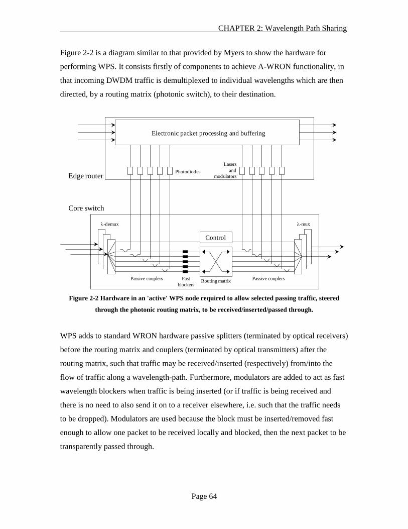
CHAPTER 2: Wavelength Path Sharing
Page 64
Figure 2-2 is a diagram similar to that provided by Myers to show the hardware for
performing WPS. It consists firstly of components to achieve A-WRON functionality, in
that incoming DWDM traffic is demultiplexed to individual wavelengths which are then
directed, by a routing matrix (photonic switch), to their destination.
Control
Lasersand
modulatorsPhotodiodes
Electronic packet processing and buffering
Edge router
Core switch
Passive couplers Fast blockers
Passive couplersRouting matrix
λ-demux λ-mux
Figure 2-2 Hardware in an 'active' WPS node required to allow selected passing traffic, steered
through the photonic routing matrix, to be received/inserted/passed through.
WPS adds to standard WRON hardware passive splitters (terminated by optical receivers)
before the routing matrix and couplers (terminated by optical transmitters) after the
routing matrix, such that traffic may be received/inserted (respectively) from/into the
flow of traffic along a wavelength-path. Furthermore, modulators are added to act as fast
wavelength blockers when traffic is being inserted (or if traffic is being received and
there is no need to also send it on to a receiver elsewhere, i.e. such that the traffic needs
to be dropped). Modulators are used because the block must be inserted/removed fast
enough to allow one packet to be received locally and blocked, then the next packet to be
transparently passed through.

CHAPTER 2: Wavelength Path Sharing
Page 65
Therefore at this node, a particular incoming wavelength-path, at a particular instant, may
be:
• Transparently passed through to the next node, as in an A-WRON intermediate
node.
• Received, and also allowed to pass through to the next node (for
multicast/broadcast applications)
• Received and blocked. That is to say, dropped.
If the wavelength-path is blocked (i.e. not being transmitted on upstream) at this node,
the part of the wavelength-path downstream of this node may optionally be used for
additional traffic from this or a later node – spatial sharing.
2.1.1 Motivation for using wavelength path sharing (WPS)
[Myers 01] analysed the efficiency achievable for different logical path lengths. In
particular, Myers proved analytically that under uniform demand a 3-node logical path
allows 100% efficiency in using every segment of its physical path. Longer logical paths
have a lower efficiency: 1
4+N
for N odd, 2
)1(4NN − for N even, where N is the number of
nodes, with efficiency measured as the bandwidth utilisation of the least-utilised link,
normalised to a link capacity of 1, with N ≥ 3. Therefore consideration is limited to a 3-
node logical path within the rest of this chapter. With this limitation, Myers analytically
proved a theoretical lower bound where WPS would use half of the wavelengths required
by an A-WRON, as judged by the Baroni theoretical lower bound. This result was for a
uniform traffic matrix, with half of one wavelength per demand.
This is a significant saving in the number of wavelengths required to serve a set of
demands, and is a further reason for considering WPS.
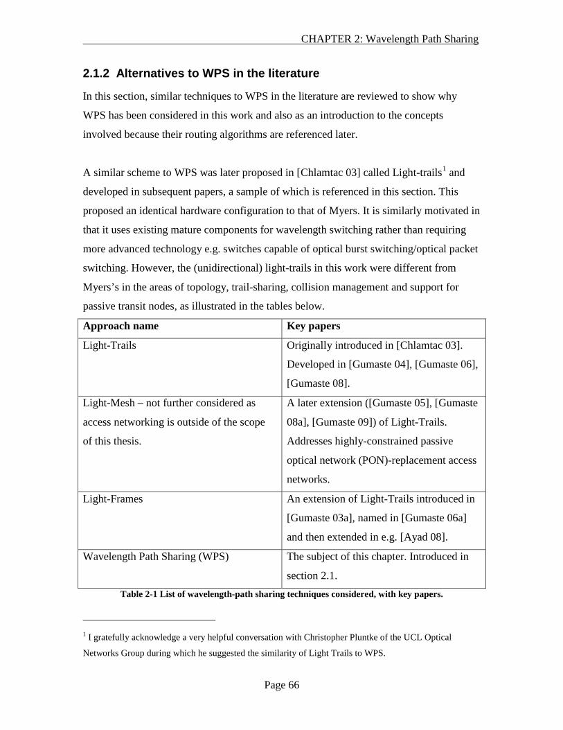
CHAPTER 2: Wavelength Path Sharing
Page 66
2.1.2 Alternatives to WPS in the literature
In this section, similar techniques to WPS in the literature are reviewed to show why
WPS has been considered in this work and also as an introduction to the concepts
involved because their routing algorithms are referenced later.
A similar scheme to WPS was later proposed in [Chlamtac 03] called Light-trails1
Approach name
and
developed in subsequent papers, a sample of which is referenced in this section. This
proposed an identical hardware configuration to that of Myers. It is similarly motivated in
that it uses existing mature components for wavelength switching rather than requiring
more advanced technology e.g. switches capable of optical burst switching/optical packet
switching. However, the (unidirectional) light-trails in this work were different from
Myers’s in the areas of topology, trail-sharing, collision management and support for
passive transit nodes, as illustrated in the tables below.
Key papers
Light-Trails Originally introduced in [Chlamtac 03].
Developed in [Gumaste 04], [Gumaste 06],
[Gumaste 08].
Light-Mesh – not further considered as
access networking is outside of the scope
of this thesis.
A later extension ([Gumaste 05], [Gumaste
08a], [Gumaste 09]) of Light-Trails.
Addresses highly-constrained passive
optical network (PON)-replacement access
networks.
Light-Frames An extension of Light-Trails introduced in
[Gumaste 03a], named in [Gumaste 06a]
and then extended in e.g. [Ayad 08].
Wavelength Path Sharing (WPS) The subject of this chapter. Introduced in
section 2.1. Table 2-1 List of wavelength-path sharing techniques considered, with key papers.
1 I gratefully acknowledge a very helpful conversation with Christopher Pluntke of the UCL Optical
Networks Group during which he suggested the similarity of Light Trails to WPS.

CHAPTER 2: Wavelength Path Sharing
Page 67
Approach
name
Light-Trails Light-Frames Wavelength
Path Sharing
(WPS)
Applicable
topologies.
2-fibre rings or unbranching lines –
no routing flexibility and so no
photonic cross-connect except for
the wavelength blocker.
No restrictions -
arbitrary mesh
No restrictions -
arbitrary mesh
Growth and
shrinking of
lightpaths
Light trails may automatically grow
and shrink along the pre-defined
constrained topologies.
No support -
routing decisions
would be needed
to extend the
trail at branching
points.
No support.
Trail-
sharing
Wavelength blockers at active
nodes are used solely to separate
semi-permanent (meaning not
moved per-packet) light-trails, not
between frames.
As a consequence, downstream
nodes are starved of transmission
opportunities by any upstream
transmitter sending traffic.
Trail-sharing could be added to this
scheme.
As Light-Trails One trail can
simultaneously
be used by two
or more frames
at once,
separated by a
modulator used
as an optical
blocker. This
increases the
traffic that may
be served.
What
happens
when more
than one
transmitter
at once has
Ethernet collisions result in invalid
frames which have to be re-sent, at
a cost of additional bandwidth and
frame latency variation. The re-
send mechanism requires nodes to
cache any received-from-upstream
As per Light-
Trails, plus
[Gumaste 06a]
requires nodes to
have a total map
of the network’s
Pre-arranged
slots. No
collisions.

CHAPTER 2: Wavelength Path Sharing
Page 68
data to
send?
frames while sending downstream,
then later re-send the upstream
frames if a collision was detected.
See the row below on the impact
this has on OEO requirements and
transparency.
topology to
determine
whether to
retransmit on a
collision or not
because the
packet may have
also taken an
alternative path –
much more
complex than
standard
Ethernet.
Scope to
reduce OEO
equipment,
bitrate and
format
transparency
To enable resending on collisions,
all receivers along the path must be
capable of all bitrates/formats that
might be used upstream of them.
Then, why not remove the photonic
bypass path altogether and act as a
2-node electronic switch at all times
at every node? While this would
increase latency of through-traffic
due to the additional processing, it
would entirely eliminate the wasted
bandwidth of Ethernet collisions,
remove the need for the related
guard times for collision detection,
and also increase optical reach as
the signal would be wholly
regenerated.
As Light-Trails Only the
originating
transmitter and
terminating
receiver are
used by any
given burst. I.e.
WPS is
completely
transparent to
the capabilities
of other devices
on the bus.

CHAPTER 2: Wavelength Path Sharing
Page 69
Support for
passive
transit nodes
(WRON-
type nodes
that don’t
participate
in per-
packet
switching)
No, but could be enhanced.
Chlamtac et al. acknowledge that
this causes inefficiency in that this
causes the centre of the light trail to
become a ‘hot-spot’ versus the links
at the ends. Including superfluous
switching introduces unnecessary
optical impairment. It is possible
that the desire for more transmitters
on the bus, and hence more scope
for opportunistic use of bandwidth,
reflects the strong preference of
statistical multiplexing versus
Myers’s slotted system.
No, but could be
enhanced. See
previous column
for further notes.
Fully supported.
Myers
recommended
using 3-node
‘trails’ to
achieve 100%
utilisation
efficiency,
which requires
passive transit
nodes if any
reasonable
reach is to be
achieved.
Broadcast
and
multicast
suitability
Larger number of nodes on a trail
makes this more effective than a 3-
node WPS logical path.
As with Light-
Trails.
3-node logical
paths slightly
more efficient
than A-WRON. Table 2-2 Comparison of wavelength path-sharing techniques
2.1.2.1 More detail on Light Frames
“Light-frames” (from e.g. [Gumaste 06a]) is now described, because it is the expansion
of light-trails to full mesh networks and so is the nearest equivalent to WPS. Light-frames
introduced the concepts of ‘strings’ (the light-trails themselves) and ‘threads’ (point-to-
point connections between nodes in different strings). Interconnection between strings
and threads may be all-optical, but the per-wavelength interconnection includes a blocker
such that the linkage may be made OEO to break optical cycles or otherwise. This allows
quite generalised directional acyclic tree bus structures, in that there may be merge/join
points between the light-trail-style topologically linear buses. Similar to the need for long
strings, no argument is offered for why this is useful. Indeed the early [Gumaste 03a]
dismisses the option as too complex. However, it offers the option to use OEO bridging
CHAPTER 2: Wavelength Path Sharing
Page 70
between strings and trails where an OOO merge point is not desirable for any reason
(such as the excessive packet collisions it might cause if it were put between two busy
lines). By comparison, WPS (the subject of this chapter) does not consider photonic
interconnection between its ‘strings’ and thus assumes that demands will be handled
photonically from their ultimate source within the photonic network to their ultimate
destination within the photonic network, thus maximising the benefit from OOO
switching.
In conclusion, while Light-Frames are not the same as WPS for the reasons described,
there seems no reason why the listed shortcomings of the former could not be addressed
(by using the per-node modulators to allow sharing of the path; to change the control
system so there were no collisions and hence no need for the re-send mechanism; to
allow in-active transit nodes) and thus make Light-Frames a generalisation of WPS.
Considering each of these limitations separately:
• Uniform traffic: It is possible to contrive traffic patterns where longer WPS paths
achieve 100% bandwidth efficiency. For example, this could be achieved by the
following pseudo code (considering normalised bandwidth units):
1. Start with a null demand matrix, i.e. yxyxD ∀∀= ,0),( where D(x, y)
is the demand from node x to node y.
2. For each path A-B-C-D amongst a given arbitrary set of 4-node logical
paths:
For each demand in {(A, B), (B, C), (C, D)}:
• D(demand) ← D(demand) + 1
• That is to say, take the simplest example of only having
demands between immediate neighbours on the logical
path.
Paths longer than 3 nodes suffer from ‘hotspots’ – that is to say, there are more
potential demands going across the central link(s) ({(A,C), (A,D), (B,C), (B,D)}
in the above example) than across each of the outermost two links ({(A,B), (A,C),
CHAPTER 2: Wavelength Path Sharing
Page 71
(A,D)} for the first link of the above example). Therefore, the demands going
across the core links must average out to be smaller than those going across the
edge links (1/4 vs. 1/3 in this example) in order to achieve 100% bandwidth
utilisation (still assuming that only one logical path serves each demand).
Such contrived or very specific cases do not fit the scope of this chapter, which is
to consider the general case, and so this possibility is not further considered.
• Multiple logical paths: If the same demand could be split across more than one
logical path, this could help to serve particularly large peak demands that did not
fit within one logical path’s bandwidth, or to compensate for the uneven
bandwidth provided by logical paths with more than 3 nodes, as per the uniform
traffic point. These are valid cases declared out of scope of this chapter for
reasons of complexity. This is because, in addition to the simple WPS case, it
would add for each logical path the parameter of the fraction of each demand it
was serving. This is without loss of generality because a larger demand that could
be split across two logical paths may be modelled as two smaller demands.
Routing algorithms devised in connection with the light-trails-based work are reviewed
later.
The remainder of this chapter will focus purely on 3-node WPS paths as the problem
which needs to be solved, as only this configuration can achieve 100% bandwidth
efficiency, as per the Myers analytical derivation. This derivation is under the particular
conditions of uniform traffic and no more than one logical path servicing each demand.
Two problems with WPS (the hardware design proposed does not achieve the goals of
photonic networking, and the M-ILP routing algorithm provided by Myers is an ILP and
hence scales poorly) are now described and solutions proposed.
CHAPTER 2: Wavelength Path Sharing
Page 72
2.2 Discussion of WPS nodal hardware
2.2.1 Discussion of Myers’s hardware proposal and identification of problems
The nodal implementation illustrated in Figure 2-1 requires that a receiver and transmitter
for each wavelength exist at each active intermediate node. In other words, the benefits of
photonic networking that involve elimination of optical-electrical-optical conversion are
not achieved, because dedicated OE and EO hardware is required anyway.
One benefit of photonic networking is still attained, that of wavelength bitrate/format
transparency.
Wavelength bitrate/format transparency would allow, for example, nodes A-D to
communicate using more-expensive transmitter/receivers (perhaps with higher speed or
longer reach) while B and C could be equipped with much cheaper transmitters/receivers
(perhaps of lower speed or shorter reach).
The commercial case study in Appendix A shows where real-world advantage has been
taken of this kind of bitrate/format transparency in a non-WPS case, allowing terminal
transmitters/receivers to be selectively upgraded from 10Gbps to 40Gbps to 100Gbps
without having to replace intermediate nodes’ equipment.
However, in WPS as defined above, all transmitters/receiver pairs along a wavelength-
path must share a common modulation format, as during some of the timeslots they will
be communicating with each other. Therefore, photonic transparency cannot be used
unless multi-rate transmitters/receivers are used. For cost reasons, multi-rate transceivers
are unlikely to be used in the bandwidth-hungry network core, even though multi-rate
modems are conceptually well-understood, as it is not cost-effective to pay for a 40Gbps-
capable transmitter and then only run it at 10Gbps, due to the significant amount of line-
card hardware that has to be dimensioned to its highest bit-rate (FEC
processing/backplane comms/client port count etc.). Network edges (where wavelength
CHAPTER 2: Wavelength Path Sharing
Page 73
capacity is not so critical, rates are lower and so the cost impact of multi-rate cards is less
prohibitive) are outside the scope of this thesis.
Therefore, for the cost reasons outlined above, the property of photonic transparency is
not usable by WPS as defined here. While it would be possible to construct a modified
form of WPS where mixed but fixed-rate transmitter/receiver pairs are used in one
wavelength-path and can only communicate with other transceivers of the same rate, and
it would be possible to operate such a network, this option is disregarded for simplicity –
the analysis presented here would present a best case in terms of bandwidth efficiency
such a network, but only for the case where all demand positioning happened to align
with the placement of different transmitter sizes, which is unlikely in practice.
2.2.2 New proposed nodal hardware layout for supporting WPS
As discussed in the previous section when considering which benefits of photonic
networking WPS offers, WPS does not allow the user to benefit from photonic
transparency and Myers’s proposed hardware configuration does not reduce the number
of OE/EO conversions in the network versus a fully electronically switched network.
This section describes an alternative nodal hardware layout which overcomes the second
problem – it shows how WPS can reduce the number of OE/EO conversions, and the
monetary/heat/space/power costs associated with them.
In order to achieve this, the transmitters/receivers must be wavelength-tunable (a
commercially realistic assumption, see Appendix A) and an additional aggregation
photonic switching layer must be placed between the WPS splitters and the receivers as
illustrated in Figure 2-3. This shows that it is possible to exploit the sub-100% duty cycle
of the receivers/transmitters in order to share them between the passive splitters/couplers.
The example in the figure shows five wavelengths being aggregated down to require only
three transmitters/receivers – rather than one per wavelength. Such a reduction introduces
a new point of blocking. However, in many practical cases, there will already have been
at least one potential blocking point in Myers’s configuration should the electronic

CHAPTER 2: Wavelength Path Sharing
Page 74
switching matrix be dimensioned to suit anything less than peak load in terms of
dropped/added traffic.
Assuming that an active node cross-connects multiple fibres, each of which has its own
pool of transmitters/receivers, the pool could be shared between all such fibres
dynamically, for further statistical multiplexing gains. Characterising these gains is
beyond the scope of this chapter, as it requires choices in terms of acceptable switch
blocking probability which is a subjective matter of policy.
Control
Lasersand
modulatorsPhotodiodes
Electronic packet processing and buffering
Edge router
Core switch
Passive couplers Fast blockers
Passive couplersRouting matrix
λ-demux λ-mux
New aggregation stage
Fewer OE/EO components
required
Figure 2-3 Illustration of a WPS active node hardware configuration proposed in this thesis using
intermediate aggregation stage to save OE/EO conversions
Alternatively, a wavelength-selective switch (WSS) (see [Takahashi 08] and [Ma 08] for
a discussion of what a WSS is) can be used instead, shown in Figure 2-4. This effectively
combines the functions of the demux/mux/passive-taps/power-balancing-
attenuators/routing-matrices and aggregating-MEMS layer all into one device.
The configuration proposed in this section does require that the transmitters, receivers
and aggregating components (such as the new routing matrix in the first figure) be
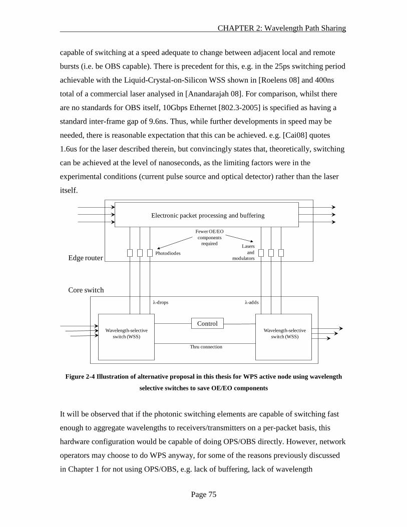
CHAPTER 2: Wavelength Path Sharing
Page 75
capable of switching at a speed adequate to change between adjacent local and remote
bursts (i.e. be OBS capable). There is precedent for this, e.g. in the 25ps switching period
achievable with the Liquid-Crystal-on-Silicon WSS shown in [Roelens 08] and 400ns
total of a commercial laser analysed in [Anandarajah 08]. For comparison, whilst there
are no standards for OBS itself, 10Gbps Ethernet [802.3-2005] is specified as having a
standard inter-frame gap of 9.6ns. Thus, while further developments in speed may be
needed, there is reasonable expectation that this can be achieved. e.g. [Cai08] quotes
1.6us for the laser described therein, but convincingly states that, theoretically, switching
can be achieved at the level of nanoseconds, as the limiting factors were in the
experimental conditions (current pulse source and optical detector) rather than the laser
itself.
Control
Lasersand
modulatorsPhotodiodes
Electronic packet processing and buffering
Edge router
Core switch
Fewer OE/EO components
required
Wavelength-selective switch (WSS)
Wavelength-selective switch (WSS)
Thru connection
λ-drops λ-adds
Figure 2-4 Illustration of alternative proposal in this thesis for WPS active node using wavelength
selective switches to save OE/EO components
It will be observed that if the photonic switching elements are capable of switching fast
enough to aggregate wavelengths to receivers/transmitters on a per-packet basis, this
hardware configuration would be capable of doing OPS/OBS directly. However, network
operators may choose to do WPS anyway, for some of the reasons previously discussed
in Chapter 1 for not using OPS/OBS, e.g. lack of buffering, lack of wavelength

CHAPTER 2: Wavelength Path Sharing
Page 76
conversion, latency requirements and network size that preclude the round-trip signalling
of WROBS.
The remainder of this chapter does not make any assumptions regarding the particular
hardware configuration used to implement WPS.
2.3 Routing algorithm proposal
2.3.1 Why is a new routing algorithm needed?
Much has been written on how to route and allocate wavelengths to serve demand
patterns with A-WRONs (e.g. [Baroni 98], [Zapata-Beghelli 08], [Belgacem 08]).
However, this task is different when considering WPS networks. Referring back to Figure
2-1: a physical path (2-1-8-9) is chosen not to support a demand directly, but to support
one of several possible logical paths (2-8-9 in this example), any of which will
simultaneously satisfy several demands; in the example given, the demand set is
{(2, 8), (2, 9), (8, 9)}. The objective is to ensure that every demand in the traffic matrix is
satisfied, and to do so using a minimum of resources. I.e. not wastefully serving some
demands multiple times or with more bandwidth than is required. For example, if, in
addition to Figure 2-1, the same network also contained logical path 7-8-9 then the
demand 8-9 is wastefully/unnecessarily served by both logical paths. Therefore, WPS
routes groups of demands, and part of the routing operation, unlike A-WRON, is to
choose an optimal set of demand-groups to route.
In his proposal Myers assessed potential network utilisation gains of WPS by
transforming the wavelength-path placement problem into an integer linear programming
problem and using standard optimisation software to gain an answer.
While ILP approaches often achieve extremely good results due to optimising an exact
formulation of the problem, they are notorious for their long execution time (because,
with bounded variables, as used in this case, they are NP-hard). However, in this
particular case, the execution time scaled up in size so rapidly that [Myers 01] had to use
a restricted formulation of the problem in order to obtain results in what he described as a

CHAPTER 2: Wavelength Path Sharing
Page 77
"reasonable period". As the results below (section 2.3.6) show, even this restricted
formulation could fail to complete within several days for large networks (43 or 46 nodes
failed to complete within four days, where networks up to 21 nodes completed in less
than twenty seconds). Therefore, to achieve a result in a reasonable time span for more
general (i.e. larger) network sizes, a more scalable heuristic is required.
[Zapata-Beghelli 08] reviewed routing and wavelength assignment (RWA) algorithms
used in existing A-WRONs, concluding that the Adaptive Unconstrained Routing with
Exhaustive wavelength consideration (AUR-E) (first proposed in [Mokhtar 98]) is the
best heuristic for routing a network in terms of reducing blocking probability. AUR-E is
very computationally intensive due to separately running the Dijkstra shortest path
algorithm for each wavelength supported in the network. However, it is still an
improvement relative to an integer linear programming (ILP) approach and incurring the
NP-hard scaling that brings (such as [Belgacem 08], although he has a technique for
reducing the scaling problem, by breaking the problem down into chunks and ILP-
solving each chunk separately). This is the intuitively expected answer for two reasons: a)
an adaptive algorithm should perform better than a static algorithm (as the former has
more information – current network state – to work on); and b) an algorithm performing
simultaneous routing and wavelength allocation has the opportunity to consider the joint
optimum between these two axes, where separate routing and wavelength allocation
phases as per Zapata-Beghelli’s alternative algorithms can only provide the combination
of optimum routing allocation with the separately-optimal wavelength allocation on those
routes. The simulation results later in this section seem to back up Zapata-Beghelli’s
conclusions as will be seen in section 2.4.5.
None of the existing RWA algorithms, which were designed for WRONs, deal with the
problem of WPS routes explicitly or serving multiple demands as used in WPS. The
nearest equivalent work to WPS is light-frames and therefore is it appropriate to review
the routing algorithms proposed in that area for suitability.

CHAPTER 2: Wavelength Path Sharing
Page 78
2.3.2 Review of Light-Frames routing algorithms
This section reviews key papers in Light-Frames work in terms of the routing algorithms
proposed and also discusses why they are not suitable for finding the best wavelength-
paths in the scenario described in this chapter.
The Light-Trails (e.g. [Chlamtac 03]) and Light-Mesh (e.g. [Ayad 08]) work describes
constrained topologies (rings or pre-planned paths) and so there are no routing decisions
to be made, merely decisions on where each Trail should be allowed to start/end (with a
semi-permanent block before/after). These assume that those constrained technologies
already exist and so do not provide routing algorithms to determine where they should be
placed.
The Light-Frames concept (e.g. [Gumaste 06a]) works on arbitrary meshes and as such it
routes paths similar to those required for WPS.
[Gumaste 06a] offered an ILP formulation for routing strings and threads. However, its
minimisation objective is for the number of strings, threads and OEO nodes (an OEO
node is just an OOO node with wavelength blocking activated, so incurring no additional
cost), rather than any direct measure of network resource usage, and so it cannot be relied
upon to produce optimal results. Similarly, [Ayad 08] provides an ILP which minimises
trails rather than wavelengths. Without a fixed trail length there is no way of directly
calculating wavelength-link usage from trail count. Indeed [Fang 04] notes that different
solutions are required to optimise wavelength-links instead of number of trails. As the
existence of more trails does not in itself cost more money, except in the number of
wavelengths it consumes, this seems the wrong optimisation; it makes more sense that
wavelength-links should be optimised directly. It would be possible to argue that using
more trails requires more transceivers/per-wavelength optics. However, this argument is
inapplicable to the Gumaste proposal because the light-trails proposal possessed
switching nodes on all available wavelengths (to allow the light-trail lengths/routes to be
dynamic). Thus, the light-trails hardware cost is actually related to the number of
wavelengths that may be used, rather than the number of trails used.

CHAPTER 2: Wavelength Path Sharing
Page 79
Therefore, as per the previous section, an algorithm is required that finds optimal logical
paths that serves multiple demands (as occurs in WPS) and, as per this section, this must
be done such that optimality is assessed in terms of wavelength-links, being a more direct
and simple measure of network capacity consumed than those which have been reviewed
in this section.
Proposal and references Topology considered Minimisation objective
Light-Trails (e.g. [Chlamtac 03]) Constrained (rings, or
pre-planned)
N/A
Light-Mesh (e.g. [Ayad 08])
Light-Frames ([Gumaste 06a]) Arbitrary mesh Count of strings, threads
and OEO nodes.
Light-Frames ([Ayad 08]) Arbitrary mesh Trail-count
This Chapter (LRF, AUR-F) Arbitrary mesh Network capacity consumed
(Wavelength-links) Table 2-3 Summary of properties of routing algorithms discussed in this section
2.3.3 New heuristic routing algorithm 1 – longest-route first (LRF)
2.3.3.1 Pseudo-code
The objective is to produce an algorithm that executes faster than the M-ILP formulation
but produces comparable results in terms of minimizing the number of wavelength-links
consumed to serve all demands. This novel heuristic algorithm, "Longest-Route First"
(LRF), outputs a list of logical paths (with supporting physical paths) that, for a given
target network topology, fully satisfy all traffic demands.
The algorithm builds on the Light-trails proposals such as [Gumaste 06]’s “Longest pair
heaviest-load assignment”, generalised to cope with a mesh topology (instead of a simple
ring), to accommodate passive transit WPS nodes, and enhanced with the analysis (of the
non-WPS case) done by [Zapata-Beghelli 06]. This algorithm shows that k-shortest-path
first-fit achieved near-optimal results at a much reduced computational cost versus the
best heuristic solution of an adaptive routing algorithm such as AUR-E [Mokhtar 97].

CHAPTER 2: Wavelength Path Sharing
Page 80
The algorithm produces logical paths of length limited to 3 nodes (as previously
discussed in this chapter, this is the limit at which 100% usage of the network may be
achieved with uniform traffic).
Within the following pseudo-code, demands are denoted by the ordered tuple (s, d),
denoting a unidirectional demand from node s to node d. Establishing a WPS logical path
(a, b, c) serves the demands (a, b), (b, c) and (a, c). Notation in square brackets denotes
computational complexity of the step, with the net effect discussed in the next section.
Pseudo-code for the LRF algorithm is:
1. Calculate the k-shortest paths between all pairs of nodes. [Demands.O(n log n)]
a. For each pair of nodes, sort the k-shortest paths such that they are in order
of increasing length (defined as number of hops in the implementation for
generality, but could also be done by link weight or geographical
distance). [Demands.O(n log n)]
b. As steps 1 and 1.a are traffic invariant, they may be done offline.
2. Sort the unidirectional traffic demands in order of decreasing distance. Define this
ordering as demand (sA, dA)< (sB, dB) if the shortest path between the nodes
(sA, dA) is shorter than the shortest path between the nodes (sB, dB
3. For each un-served traffic demand (s, d) in the list, in order (as sorted in the
previous step):
). [O(n log n)]
a. For each path identified in the previous step of length greater than 2 nodes,
find the central node of the path and designate this as both q and r. If the
centre of the path falls between two nodes, designate one node q and the
other r.
i. Test if r is such that the demands (s, r) and (r, d) have not yet
already been met. If that is the case, establish the WPS logical path
(s, r, d) and go back to step 3 to consider the next demand (s, d). If
only one of those demands has not been met, set b= r and continue
to step ii.

CHAPTER 2: Wavelength Path Sharing
Page 81
ii. Test if q is such that the demands (s, q) and (q, d) have not yet
already been met. If that is the case, establish the WPS logical path
(s, q, d) and go back to step 3 to consider the next demand. If only
one of those demands has not been met, set b=r and continue to
step iii.
iii. Move r one hop along the path towards d. Move q one hop along
the path towards s. Go to step i.
iv. Once both ends have been reached go back to step a, and then
consider the next path in the list.
v. Once all paths have been considered, if a match has not already
been found as per steps i or ii, if a partial match node (b) has been
found then establish a WPS logical path (s, b, d). If no such partial
match was found, establish a sub-length WPS logical path of (s, d).
b. Go back to step 3 and consider the next demand (s, d) in the list.
Step 3 will terminate when all demands have been served.
It is assumed that the network is fully connected, i.e. that no (s, d) exist such that there is
no possible path from s to d. This assumption is without loss of generality, as any
demands between the partitions of a disconnected network are not directly serviceable
and so must be dealt with by a means other than WPS.
Note: Where wavelength allocation is also considered, as described in section 2.4
onwards, an additional heuristic (AUR-F) doing simultaneous routing and wavelength
allocation is proposed in section 2.4.3.
CHAPTER 2: Wavelength Path Sharing
Page 82
2.3.3.2 Algorithm execution complexity
The computational complexity of the action in each step is marked next to it. However,
there are multiple parts to step 3, so the net total complexity of this must be calculated, as
follows:
• Assume there are n2
• The k-shortest paths of step
demands as is the worst case, achieved by e.g. a uniform
traffic demand.
1 must therefore be executed n2 times, resulting in a
complexity of O(n3
• Step
log n).
1.a likewise has complexity O(n3
• There are at worst, n
log n). 2 3 iterations of step .
• The k iterations of step a (due to the k shortest paths) may be disregarded for
scaling analysis, being a constant.
• As a result, steps i-v just iterate along the length of a path l, O(l).
• Therefore, step 3 costs O(n2
Each iteration of step
.l).
3 may address up to three separate demands, but this just introduces
another constant factor which should be ignored for worst-case complexity analysis.
Therefore step 1 dominates the complexity, so the LRF algorithm achieves a complexity
of O(n3
However, if step
log n).
1 and 1.a may be executed in advance, then the processing for each
demand as it arrives is much reduced such that only steps 3.a.i-3.a.v need be executed.
Therefore, in normal usage, the complexity of the LRF algorithm is O(n2
2.3.4 Objective of the simulation
.l), where l is the
average length of the optical path.
The objective of the simulation is to compare the performance of the LRF algorithm with
the M-ILP formulation. In this section, performance is measured in terms of the number
of wavelengths consumed (Nλ in the results below) for consistency and comparison with

CHAPTER 2: Wavelength Path Sharing
Page 83
Myers’s results. An alternative approach of considering performance in terms of
continuous wavelengths is described and pursued in section 2.4 onwards, to which this
first simulation is an approximation.
As a benchmark, the A-WRON lower bound of wavelengths required for the same
network is found, as derived in [Baroni 98].
2.3.5 Simulation conditions/assumptions
A uniform traffic model is assumed, for comparability with Myers’s results, with an
average of 0.5 wavelengths per (source, destination) node pair, and no traffic starting and
terminating at the same node (as the access layer will directly switch that traffic). The
traffic model is static throughout this chapter: changing traffic is discussed in the next
chapter. As per Myers, these are the best-case conditions for 3-node WPS paths – where
they should achieve 50% cost-savings versus A-WRONs.
The networks simulated are the standard analysis networks taken from [Zapata-
Beghelli 06] shown in Appendix B (as are the other simulations performed in this thesis).
The choice of these topologies, and their characteristics, are described there.
Demands are routed unprotected, as per the assumption stated in Chapter 1. This is also
to remain consistent with Myers in order to allow the results to be compared.
2.3.6 Results of simulations
With ε = 1 or 2, the M-ILP [Myers 01] failed to run to completion within a few days, it
was necessary to limit ε at 0. This will have affected the results for the worse, as it
constrains the M-ILP to only considering shortest paths. Myers also had to use ε = 0 for
some of his runs where ε = 1 failed to terminate ‘in a reasonable time’. The difficulty of
getting these results is a practical demonstration of the unsuitability of an ILP approach to
practical usage on larger networks due to execution time.

CHAPTER 2: Wavelength Path Sharing
Page 84
Simulations were run, for each network, using the following parameters:
N Number of nodes
L Number of links
α The normalized number of bi-directional links with respect to a fully-
connected mesh topology (as defined in Appendix B).
∆ The mean nodal degree in the graph
Nλ (A-WRON) Minimum number of wavelengths that would be required to serve the
demands by an A-WRON according to the Baroni lower bound.
Nλ (M-ILP) Minimum number of wavelengths that would be required to serve the
demands by WPS, calculated according to Myers’s ILP (M-ILP)
Nλ (LRF) Minimum number of wavelengths that would be required to serve the
demands by WPS, calculated according to the LRF algorithm
proposed in this chapter.
Table 2-4 Key parameters used in this chapter. This information is a subset of the List of symbols at
the front of the thesis.
Benchmark
Tor3 9 18 0.5 4 3 2 66.67% 4 133.33%Eurocore 11 25 0.45 4.55 4 3 75.00% 5 125.00%NSFnet 14 20 0.22 2.86 13 8 61.54% 10 76.92%EON 20 39 0.21 3.9 18 9 50.00% 15 83.33%UKNet 21 39 0.19 3.71 19 11 57.89% 14 73.68%ArpaNet 20 31 0.16 3.1 33 17 51.52% 22 66.67%
N L
Network parameters Existing ILP Proposed heuristic
Networkα
(2d.p.)∆
(2d.p.)Nλ
(M-ILP)
Nλ(M-ILP) / Benchmark
%Nλ
(LRF)
Nλ (LRF) /
Benchmark
%
Non-WPS benchmark
Nλ(A-WRON)
Table 2-5 Comparison of LRF with M-ILP and A-WRON
The LRF also used ε to indicate the maximum permitted deviation from the shortest path.
The optimal value of ε varied per network, so the algorithm discussed henceforth is
where the LRF is executed with ε = 0 then ε = 1 then ε = 2 in sequence and the best result

CHAPTER 2: Wavelength Path Sharing
Page 85
chosen. A maximum value of ε = 2 was chosen, as higher values do not appear to give
any significant improvement.
The results of the LRF heuristic relative to M-ILP, compared to the calculated Baroni
lower bound are provided in Table 2-5.
With the USNet (46 nodes/76 links) and Eurolarge (43 nodes/90 links) network
scenarios, M-ILP failed to run to completion after approximately four days of execution
time (each), reinforcing the need for a new heuristic, e.g. LRF, for networks of practical
size.
0
5
10
15
20
25
30
35
Tor3 Eurocore NSFnet EON UKNet ArpaNet
Hig
hest
wav
elen
gth
coun
t on
any
link
in t
he n
etw
ork
Network
Non-WPS benchmark Nλ (A-WRON)
Nλ (M-ILP)
Nλ (LRF)
Figure 2-5 The performance of the LRF heuristic algorithm versus Myers's ILP (M-ILP) and the
Baroni lower bound in terms of the number of wavelengths consumed.

CHAPTER 2: Wavelength Path Sharing
Page 86
[Myers 01] proves (by trivial analytical derivation) that the theoretical minimum
achievable number of wavelengths required, relative to an A-WRON, is 50%.
The results from the table are shown in graphical form in Figure 2-5. The network graphs
are ordered in terms of increasing Nλ (A-WRON), which for these graphs is the same as
decreasing alpha. This is an arbitrary sorting.
The reason for using a heuristic algorithm was to decrease the processing time required.
Table 2-6 shows the measured time in achieving the results above for each method over
each graph. Note that a non-trivial amount of time is spent formulating the M-ILP before
it can be fed to the solver, because the problem formulation requires all possible logical
and physical paths to be enumerated. For clarity, these times have been displayed
separately.
These results were produced using an (otherwise unloaded) Intel T2050 1.6GHz running
Windows XP Media Center SP3 with 1.5Gb of RAM, averaged over three runs.
Execution times did not vary significantly over the three runs.
Tor3 9 18 0.5 4 0.05 0.01 0.01 0.05 310.87%Eurocore 11 25 0.45 4.55 0.24 0.02 0.03 0.1 221.99%NSFnet 14 20 0.22 2.86 0.32 0.03 0.03 0.12 193.55%EON 20 39 0.21 3.9 5.55 0.12 2.63 0.52 18.79%UKNet 21 39 0.19 3.71 11.22 0.13 1.88 0.55 27.47%ArpaNet 20 31 0.16 3.1 3.43 0.1 1.53 0.39 23.64%
Network data Existing ILPA-WRON execution
time(seconds)
(2d.p.)[for interest
only]
Proposed algorithm
(LRF) execution
time (seconds)
(2d.p.)
Proposed (LRF) vs. Existing (M-ILP) (total time)
% (2d.p.)Network α (2d.p.) ∆ (2d.p.)
M-ILP prep time (seconds)
(2d.p.)
M-ILP execution
time (seconds,
2d.p.)N L
Table 2-6 Execution time of the different algorithms considered over standard analysis networks

CHAPTER 2: Wavelength Path Sharing
Page 87
2.3.7 Analysis and discussion of simulation results
M-ILP only achieved the Myers theoretical exact lower bound (on performance of 50%
with 3-node paths) with the EON network, but not with other networks. Nonetheless,
both M-ILP and LRF achieve an improvement over the non-WPS A-WRON value,
showing that WPS is providing benefit.
As would be expected, LRF provided less optimal results than the M-ILP formulation
benchmark (an average of approximately 50% more wavelengths). However it is
significant that, for the larger networks where efficiency is more important, the LRF
heuristic is still bettering (by 17-33%) the A-WRON theoretical lower bound (as well as
running to completion within a reasonable time period, even on networks where M-ILP
did not). Using A-WRON, this theoretical bound is not always achievable in practice, or
with a practical algorithm, making the improvement demonstrated here more significant.
For general use, both algorithms (M-ILP and LRF) should be modified such that they
never achieve a worse result than A-WRON, as there is no advantage to WPS except in
terms of saved wavelengths. A simple way of doing this would be to run a (reasonably
optimal) A-WRON routing algorithm at the same time and use whichever result produced
the lower wavelength count.
Both of these routing algorithms (M-ILP and LRF) always use a 3-node logical path if
one is physically possible, ignoring more efficient 2-node options, resulting in sub-
optimal results in some situations. This is justified as, when consuming the same number
of links, 3-node paths are preferable over 2-node paths because they serve 3 demands
rather than 1. However, one 3-node path consuming x links is clearly less efficient than
three 2-node paths averaging < x/3 links each. A more-optimal WPS placement would
have the A-WRON lower-bound wavelength-count as its upper bound: A-WRON point-
to-point wavelengths can be considered 2-node logical paths and thus a sub-part of the
optimization-space that the WPS route-placer is considering.

CHAPTER 2: Wavelength Path Sharing
Page 88
The heuristic can be judged as a success in that, where an ILP performs poorly (if at all,
in the case of larger networks), LRF is able to show significant (>20%) value for WPS
while saving a significant (70-80%) proportion of the execution time. This advantage in
execution time would increase with larger networks to the point where the LRF would get
results where the ILP did not complete within reasonable time.
With smaller networks (where execution time is less of an issue), LRF did take longer to
execute but this is believed to be due to a lack of optimisation in the start-up of the
heuristic execution. It is expected that further work could eliminate this anomaly.
It should be noted that, in most of these cases, M-ILP does not achieve its theoretical
50%, which may be due to the limited value of ε=0 (required for reasonable execution
time as discussed in section 2.3.6). Increasing ε is likely to improve the M-ILP’s results at
a cost of increase execution time.
The purpose of the LRF algorithm and these simulations was to provide and prove a
faster and more scalable alternative to M-ILP, which both calculate routing. However,
routing without wavelength allocation does not fully account for wavelength-links
consumed. The next section describes why this is the case, proposes an additional new
routing algorithm with wavelength allocation (AUR-F) and compares its bandwidth
efficiency to those already seen in the simulations discussed so far in this chapter.
2.4 The effect of wavelength allocation and why it is important to consider wavelength continuity and unique wavelengths
In the previous section, two routing algorithms (M-ILP and LRF) are compared for
performance in terms simply of the maximum number of wavelength-links required on
any link. The choice of simulation conditions allows comparison with Myers’s results.
However, as WPS does not include wavelength conversion, it must in practice use one
frequency of light along the whole route of each wavelength-path (the wavelength
continuity constraint, as defined in Chapter 1). Because of the possibility of blocking (a
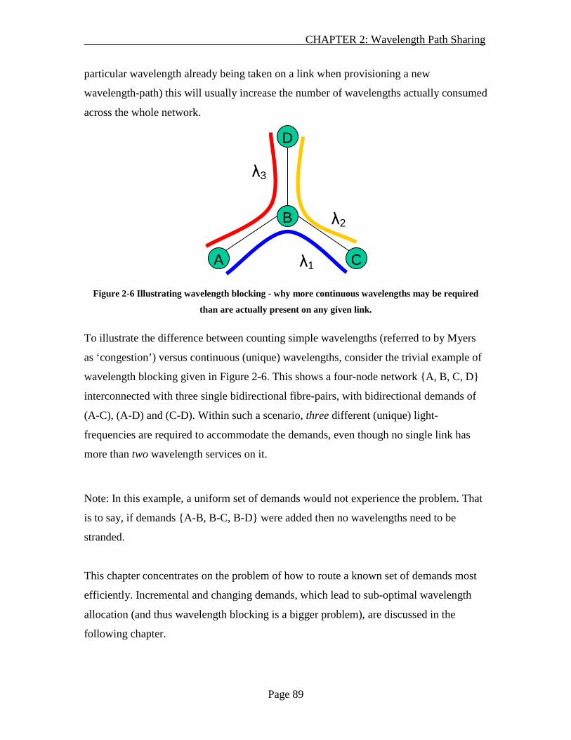
CHAPTER 2: Wavelength Path Sharing
Page 89
particular wavelength already being taken on a link when provisioning a new
wavelength-path) this will usually increase the number of wavelengths actually consumed
across the whole network.
Figure 2-6 Illustrating wavelength blocking - why more continuous wavelengths may be required
than are actually present on any given link.
To illustrate the difference between counting simple wavelengths (referred to by Myers
as ‘congestion’) versus continuous (unique) wavelengths, consider the trivial example of
wavelength blocking given in Figure 2-6. This shows a four-node network {A, B, C, D}
interconnected with three single bidirectional fibre-pairs, with bidirectional demands of
(A-C), (A-D) and (C-D). Within such a scenario, three different (unique) light-
frequencies are required to accommodate the demands, even though no single link has
more than two wavelength services on it.
Note: In this example, a uniform set of demands would not experience the problem. That
is to say, if demands {A-B, B-C, B-D} were added then no wavelengths need to be
stranded.
This chapter concentrates on the problem of how to route a known set of demands most
efficiently. Incremental and changing demands, which lead to sub-optimal wavelength
allocation (and thus wavelength blocking is a bigger problem), are discussed in the
following chapter.
A
B
C
D
λ1
λ2
λ3

CHAPTER 2: Wavelength Path Sharing
Page 90
It is important to evaluate the number of continuous unique wavelengths (light
frequencies) rather than simply the number of occupied wavelengths because it is the
exhaustion of the former which causes blocking, and thus for money spent on capacity
upgrades.
For example, the Ciena line system described in Appendix A is sold as supporting 88
wavelengths on the C-band. If this equipment had 60 wavelengths in use, but a new
demand could not be placed on this fibre due to wavelength blocking, then the operator
would be faced with the choice of deploying an additional fibre or L-band amplifier
upgrades (both incurring capital expenditure). Alternatively, a less-preferable route with
available capacity could be used, accelerating capacity blocking elsewhere in the
network.
Therefore, the two routing algorithms (M-ILP and LRF) are now compared again using
the performance measure of continuous wavelengths, based on the following
assumptions:
2.4.1.1 Assumption: No wavelength conversion
Full wavelength conversion (at all nodes in the network, all incoming wavelengths may
be translated to a different frequency before egress) eliminates the possibility of
wavelength blocking, and the relevance of this section, but adds cost. For example,
[Pedro 09] discusses the current technical immaturity of all-optical wavelength
conversion, leading to the need for expensive electro-optical (O-E-O) wavelength
conversion. The option of full wavelength conversion (meaning that the output of every
switch may convert wavelengths, which if this is done electro-optically means full OEO
at every switch and so no photonic pass-through at all) is therefore not compatible with
the objective of this thesis to investigate fully-photonic networking.
The effect of partial wavelength conversion (where wavelength converters are deployed
selectively to ease congestion) depends on how the converters are placed through the
network. e.g. [De 07] compares several approaches and presents strong simulator-based

CHAPTER 2: Wavelength Path Sharing
Page 91
evidence for an 8-15% improvement for their own proposal. Therefore, for simplicity and
generality, partial conversion is declared out of scope.
2.4.1.2 Assumption: No parallel fibres required
For the same total capacity, n parallel fibres between the same pair of nodes decreases
wavelength blocking because each light-frequency can be sent n times before blocking
occurs. [Baroni 98] section 3.8 shows this analytically.
No parallel fibres are assumed for simplicity of interpreting the results and generality –
not introducing the granularity arrangements of a particular system.
In my industrial experience, this also best represents today’s deployed networks. This is
because larger demands (those more than a significant fraction, say 10% of the size of the
wavelength) will be allocated dedicated wavelengths or fibres. Thus, the agile network is
only serving smaller demands.
Thus, and also after considering leasing-out and glass-through connections, it is
reasonable to assume that many fibres may be lit in a duct without any particular sub-
wavelength network (such as the WPS network considered here) having more than one
fibre to a particular destination.
2.4.1.3 Assumption: Wavelength exhaustion has not been reached
for any fibre
As with the no-parallel-fibres assumption (above), this is to retain generality by avoiding
introducing the granularity chosen by any particular line system; instead keeping it a
simple linear utility function, the count of continuous wavelengths.
This would be realistic for existing single-fibre-pair networks wanting to delay the
expense of lighting/adding parallel fibres. It is a loose upper-bound for multi-fibre
networks which will be less prone to blocking as discussed above. Networks with a few

CHAPTER 2: Wavelength Path Sharing
Page 92
parallel fibres added in hot-spots will perform noticeably better than discussed here as the
hot-spots are where wavelength blocking is most likely to occur. This is discussed in
[Baroni 98] section 3.8.
2.4.1.4 Assumption: Consistent line systems on all links
The objective of this simulation is to minimise the maximum number of continuous
wavelengths used by any link.
This would be an inappropriate metric if the network consisted of a mix of links of
dissimilar wavelength capability (e.g. some supporting 44 wavelengths and some
supporting 88). However, as per the previous assumptions, this would require building in
a particular granularity model which would decrease the generality of the results and so
this factor is disregarded.
This assumption is justified in terms of modern line-systems, such as the Ciena system
described in Appendix A, that do not have any fixed-frequency components (once a fibre
span has amplifiers it can carry any supported C-band wavelength). However, older
systems with fixed demultiplexing filters may support/require progressive upgrades in
order to add further bands/groups of e.g. 4 or 8 wavelengths, so deferring the expense of
the additional group filters would be beneficial versus the results shown here.
Again, introducing such system-specific details would lose generality of the results
derived later.
2.4.2 New wavelength allocation ILP formulation (WA-ILP)
This section describes a new ILP formulation (WA-ILP) that allocates specific
continuous wavelengths to a given set of routes, on a given single-fibre-per-link network.
This ILP formulation provides optimal wavelength allocation in terms of the number of
wavelength-links consumed. This optimal allocation is required to provide a lower bound
of wavelength usage to compare against the algorithms proposed in later sections. WA-
ILP is not itself considered to be practical for online use because, as with all ILPs, it is an
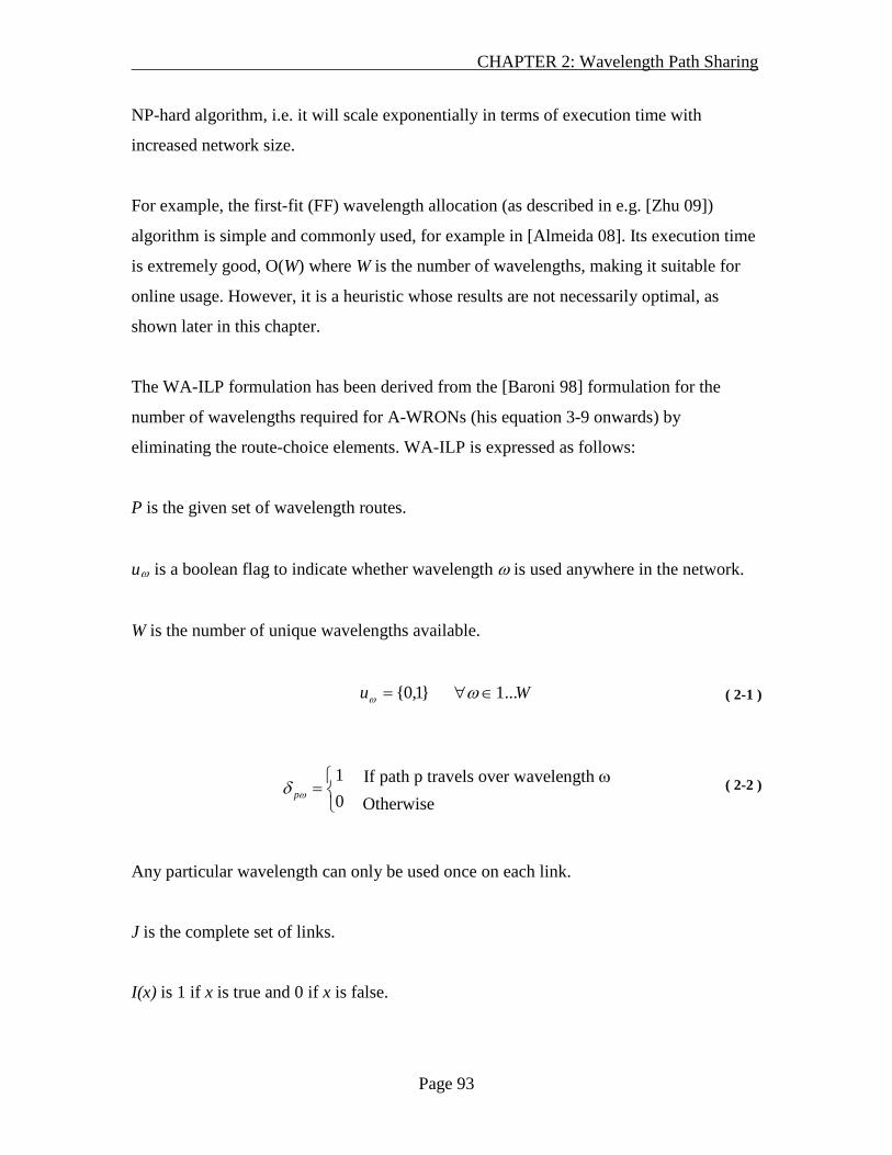
CHAPTER 2: Wavelength Path Sharing
Page 93
NP-hard algorithm, i.e. it will scale exponentially in terms of execution time with
increased network size.
For example, the first-fit (FF) wavelength allocation (as described in e.g. [Zhu 09])
algorithm is simple and commonly used, for example in [Almeida 08]. Its execution time
is extremely good, O(W) where W is the number of wavelengths, making it suitable for
online usage. However, it is a heuristic whose results are not necessarily optimal, as
shown later in this chapter.
The WA-ILP formulation has been derived from the [Baroni 98] formulation for the
number of wavelengths required for A-WRONs (his equation 3-9 onwards) by
eliminating the route-choice elements. WA-ILP is expressed as follows:
P is the given set of wavelength routes.
uω
is a boolean flag to indicate whether wavelength ω is used anywhere in the network.
W is the number of unique wavelengths available.
Wu ...1}1,0{ ∈∀= ωω ( 2-1 )
( 2-2 )
Any particular wavelength can only be used once on each link.
J is the complete set of links.
I(x) is 1 if x is true and 0 if x is false.
If path p travels over wavelength ω Otherwise
=01
ωδ p
CHAPTER 2: Wavelength Path Sharing
Page 94
∑∈
∈∀∈∀≤∈Pp
p WJjpjI ...11)( ωδ ω ( 2-3 )
Each path must be assigned a wavelength.
∑∈
∈∀≥W
p Ppω
ωδ 1 ( 2-4 )
uω
must be set if any path uses the wavelength ω:
∑∈
∀≤Pp
p u ωδ ωω ( 2-5 )
And the overall purpose of the optimisation is to perform wavelength allocation whilst
minimising the total number of wavelengths used in the network:
Objective: ∑∈
=W
uNω
ωλmin ( 2-6 )
W must be set to a number of wavelengths large enough to allow a feasible solution, and
thus for the ILP to terminate successfully. Values of W larger than strictly necessary to
allow a solution result in a longer execution time but do not affect the resulting count.
2.4.3 New heuristic routing algorithm 2 – Adaptive unconstrained routing with fixed wavelength sequence allocation (AUR-F)
The LRF and M-ILP routing algorithms previously discussed have required a separate
second phase of wavelength allocation. Separating these phases has been shown
[Mokhtar 98] to reduce efficiency of the routes produced. A novel algorithm is presented
in this section, extending Mokhtar’s work to apply to WPS, to choose the route and
wavelength simultaneously. It will be shown that this algorithm achieves substantially
greater efficiency (approximately 50% wavelength saving) versus LRF with a subsequent
wavelength allocation phase.

CHAPTER 2: Wavelength Path Sharing
Page 95
The proposed algorithm is based on the Adaptive Unconstrained Routing with Exhaustive
wavelength allocation (AUR-E) as proposed in [Mokhtar 98]. This was found to be the
most efficient (as measured in terms of blocking probability) A-WRON RWA algorithm
in Mokhtar’s paper and, in a broader comparison, more recently [Zapata-Beghelli 06].
Defining the terms used in this name:
• Adaptive means that the route the algorithm chooses will depend on current
network usage. This is as opposed to Fixed routing which is traffic unaware and
thus solely dependent on the static network topology.
• Unconstrained is as opposed to Alternate routing. In Alternate routing, multiple
routes are calculated from the static network topology, and then those for which
there is inadequate free capacity are eliminated to leave zero or more choices.
Unconstrained routing is not limited to a set of routes and so will always find a
route if one exists for which there is capacity on the network.
• Exhaustive wavelength allocation means that the demand is routed on all
wavelengths and the shortest path chosen.
As the Exhaustive wavelength allocation variant of this algorithm executes by
considering every possible wavelength, it assumes that demands are being applied to a
particular finite set of wavelengths. However, the objective problem statement of this
chapter while closely related to that is slightly different – the minimisation of the number
of wavelengths required to support a given set of demands. Therefore, the Fixed
wavelength allocation sequence variant is used instead (AUR-F) as being suitable for an
unconstrained number of wavelengths. [Mokhtar 98] showed that this produced nearly
the same results as AUR-E (he did not provide particular numbers, but his graphs make a
strong case), while being substantially lower in execution complexity (between 36% and
58% in the examples provided). This execution time advantage increases with the number
of wavelengths available as AUR-F can visit fewer where AUR-E must visit all of them
but decreases with rising blocking probability as where the network fill is higher, AUR-F
will block on earlier wavelengths and so have to visit more in total).

CHAPTER 2: Wavelength Path Sharing
Page 96
2.4.3.1 Pseudo-code
The AUR-E algorithm outputs a list of logical paths - with supporting physical paths
allocated to a particular wavelength - that fully satisfies all traffic demands on a given
network topology. The objective is to produce an algorithm that executes faster than M-
ILP combined with WA-ILP while producing comparable results.
Demands are denoted by the ordered tuple (s, d), denoting a unidirectional demand from
node s to node d. Establishing a WPS logical path (a, b, c) serves the demands (a, b), (b,
c) and (a, c). w denotes a wavelength from the set of wavelengths W.
It will be observed that this algorithm is very similar to LRF (Section 2.3.3), the critical
difference being the sequential wavelength allocation in steps 3a, 3c and 3d. Further, only
considering shortest paths is equivalent to setting ε to zero. However, as AUR-F accepts
the first path for which there is free capacity, and the path calculation is performed on
available capacity, paths with ε > 0 would never be considered. Therefore, this constraint
does not affect the results.
Pseudo-code for the algorithm is: [Notation in square brackets denotes computational
complexity of the step, with the net effect discussed in the next section]
1. Calculate the shortest path between each node. As this is traffic invariant, it may
be done offline. [O(n log n)]
2. Sort the unidirectional traffic demands in decreasing order, where ordering is
defined as demand (sA, dA)< (sB, dB) if the shortest path between the nodes (sA,
dA) is shorter than the shortest path between the nodes (sB, dB
3. For each un-served traffic demand (s, d) in the list, in order:
). [O(n log n)]
a. w ← 0
b. Calculate all shortest paths (s, d) based on current available capacity for
wavelength w. [O(n log n) ]
c. Execute step 3a of the LRF heuristic previously described in section
2.3.3.1

CHAPTER 2: Wavelength Path Sharing
Page 97
i. If a path has been found go back to step 3 of this algorithm to try
the next demand. [O(ln n) – the only loop is over the length of a
path, times the number of paths found in the previous step]
d. As a satisfactory path has not yet been found: w ← w + 1
e. Go to a and consider the next demand in the list.
Step 3 will terminate when all demands have been served.
As with LRF, it is assumed that the network is fully connected. I.e. that no (s, d) exist
such that there is no path from s to d. As before, this is assumed without loss of generality
as any demands between the partitions of a disconnected network are not serviceable and
so must be dealt with by another means than WPS.
2.4.3.2 First-fit (FF) algorithm execution complexity
As mentioned, neither M-ILP nor LRF perform wavelength allocation (they just route
traffic) and hence both require a second algorithm to perform wavelength allocation.
AUR-F does wavelength allocation simultaneously with finding routes. Therefore, it is
not appropriate to compare AUR-F’s execution time to either M-ILP or LRF directly: the
additional cost of the wavelength allocation step should be considered.
The FF (first-fit, referenced in section 2.4.2) algorithm has a complexity of O([W].[P].l)
where:
• [W] is the number of wavelengths supported by the line system (a constant
factor) to be iterated over;
• [P] is the number of paths to be wavelength-allocated, assumed to be O(n2
• l is the average path length as, for each iteration over a wavelength for a path, the
algorithm must check whether a particular link is used. If a simple sparse matrix
is used with indices of <wavelength, start node, end node> each lookup is of
constant time. More storage-efficient techniques would (probably) be preferable,
) here
– the worst case of a full mesh of demands (divided by the constant factor of
three demands served by each WPS logical path).

CHAPTER 2: Wavelength Path Sharing
Page 98
however, as a sparse matrix would require exactly [W].n2
Therefore, the net complexity of using FF as the wavelength allocation stage after either
M-ILP or LRF is O(n
elements. l can be
approximated to log n.
2
2.4.3.3 AUR-F execution complexity
log n). However, as this is done in sequence after the routing
algorithm, not within any kind of iteration, it can be ignored as this is of smaller order
than the routing algorithm itself.
The additional loop over wavelengths of step 3a, 3d, 3e mean that AUR-F has higher
complexity than the LRF algorithm. However it does eliminate the need for the
wavelength allocation step.
As will be seen in this derivation, the largest-scaling step is step 3; steps 1 and 2 are
negligible by comparison. The same worst-case assumption can be made as is made in
section 2.3.3.2, namely that the worst-case number of demands is n2
3
, giving this number
of iterations of step . The worst case number of iterations around steps 3a/3d/3e is [W],
which is a constant factor for any particular network and so can be disregarded. Step 3b
includes the O(n log n) shortest path calculation, which dominates the other steps.
Therefore, the net complexity is O(n2.[W].n log n) = O(n3
While the first few steps can be pre-calculated as with LRF. Because AUR-F is adaptive
(performs its routing calculation based on current network usage), its key routing stage
(
log n).
Therefore, AUR-F scales just as well as LRF with network size, meaning comparison
between them can be solely on bandwidth efficiency.
3.b) is within the per-demand loop, therefore pre-calculation can reduce the absolute
time, but not the scaling. With pre-calculation, complexity is therefore still O(n3 log n).

CHAPTER 2: Wavelength Path Sharing
Page 99
2.4.4 Conditions for wavelength-aware simulations
Having described a set of algorithms (M-ILP, LRF and AUR-F), wavelength allocation
approaches (WA-ILP and FF), and network assumptions, the bandwidth efficiency of
each algorithm is now compared by simulation to determine the most efficient algorithms
and also to illustrate the difference between this and the non-wavelength-continuous case
studied before in section 2.3.6.
The same networks and traffic demands as the previous (non-continuous wavelength)
simulations were used.
For WA-ILP, W was set to the output count from the FF algorithm (briefly described in
section 2.4.2) – a known feasible solution and thus meeting the "large enough"
requirement, as well as being available from a previous stage of the simulation. It is also
a practical real-world source because FF executes in negligible time compared to the
WA-ILP solution.
As will be seen from the results, a more aggressive choice of W may have been both
possible and beneficial in decreasing execution time. However, as the choice of W does
not affect the count of wavelengths produced (which was the objective), this effect was
not further investigated.
2.4.5 Simulation results and discussion
The results shown in this section compare a count of unique wavelengths used in the
network (not just the maximum count of wavelengths used across all links separately –
see section 2.4 for an explanation of this distinction) for all of the algorithms discussed
thus far in the chapter. Specifically, results are compared for:
- The routing algorithms used in the previous simulations (the LRF heuristic and
M-ILP)
- The WA-ILP and FF heuristic wavelength allocation algorithms as applied to both
routing algorithms.
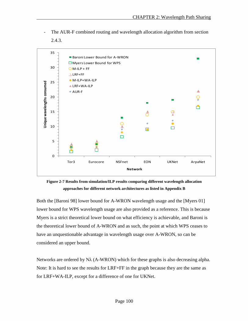
CHAPTER 2: Wavelength Path Sharing
Page 100
- The AUR-F combined routing and wavelength allocation algorithm from section
2.4.3.
0
5
10
15
20
25
30
35
Tor3 Eurocore NSFnet EON UKNet ArpaNet
Uni
que
wav
elen
gths
con
sum
ed
Network
Baroni Lower Bound for A-WRON
Myers Lower Bound for WPS
M-ILP + FF
LRF+FF
M-ILP+WA-ILP
LRF+WA-ILP
AUR-F
Figure 2-7 Results from simulation/ILP results comparing different wavelength allocation
approaches for different network architectures as listed in Appendix B
Both the [Baroni 98] lower bound for A-WRON wavelength usage and the [Myers 01]
lower bound for WPS wavelength usage are also provided as a reference. This is because
Myers is a strict theoretical lower bound on what efficiency is achievable, and Baroni is
the theoretical lower bound of A-WRON and as such, the point at which WPS ceases to
have an unquestionable advantage in wavelength usage over A-WRON, so can be
considered an upper bound.
Networks are ordered by Nλ (A-WRON) which for these graphs is also decreasing alpha.
Note: It is hard to see the results for LRF+FF in the graph because they are the same as
for LRF+WA-ILP, except for a difference of one for UKNet.

CHAPTER 2: Wavelength Path Sharing
Page 101
Network
Baroni
Lower B
ound fo
r A-W
RON
Mye
rs Lo
wer Bound f
or WPS
M-IL
P + FF
LRF+
FF
M-IL
P+WA-IL
P
LRF+
WA-IL
P
AUR-F
Tor3 3 1.5 3 4 2 4 3Eurocore 4 2 4 5 3 5 3NSFnet 13 6.5 11 10 8 10 9EON 18 9 14 15 9 15 11UKNet 19 9.5 15 15 11 14 12ArpaNet 33 16.5 20 22 17 22 19
Table 2-7 Bandwidth efficiency comparison of simulations considering allocation of unique
wavelengths. Myers lower bound should be rounded up to the nearest integer for comparisons, as a
non-integer value is not achievable in a real system.
Comparing FF to WA-ILP: Judging from the simulations results shown in Table 2-7, FF
is an excellent choice of wavelength allocation algorithm to use in association with LRF
if WA-ILP proves unacceptably slow (as networks increase in size) because FF achieves
very similar results (just one more wavelength consumed over all of the test networks
used, averaging to a ‘cost’ in bandwidth efficiency of 1% for using this much more
scalable heuristic).
However, when using M-ILP, the penalty for using FF instead of WA-ILP is higher;
averaging around 38%. If the user is using an ILP for routing then they are presumably
less concerned about execution time than a user executing a heuristic algorithm, so given
these results, it would seem more sensible to also use an ILP wavelength allocation
algorithm.
Notably, for these uniform all-to-all traffic patterns and WA-ILP, the number of unique
wavelengths required is the same as the count of wavelengths required calculated in the
previous section – WA-ILP has achieved the perfect lower bound result in these cases.

CHAPTER 2: Wavelength Path Sharing
Page 102
It should be noted that the first fit algorithm behaves (relatively) better (approx 37%)
with the routes produced by LRF versus the routes calculated by M-ILP. This may affect
many of the conclusions, e.g. [Almeida 07] [Almeida 08], drawn in the literature from
running tests with first-fit and no other validation.
2.4.6 M-ILP versus LRF versus AUR-F comparison
The routing algorithms included in Table 2-7) are compared in this section. The FF
results are ignored because the WA-ILP can be taken as providing optimal wavelength
allocation.
LRF+WA-ILP is able to offer an approximately 25% saving versus the Baroni lower
bound for the larger networks, delivering a significant fraction of the benefit of WPS as
benchmarked by M-ILP+WA-ILP.
M-ILP+WA-ILP offers a 25-50% gain over the A-WRON, clearly demonstrating the
potential for WPS to save wavelengths, and achieves the Myers lower bound for WPS in
half the cases (as fractional wavelength counts must be rounded up to integers in
practice). However, being NP-hard, it does not necessarily complete within a reasonable
time.
AUR-F offers a significant improvement over LRF+WA-ILP (averaging 22% of its
wavelengths) and critically, is always at least as good as the A-WRON Baroni lower
bound. It does not quite reach the performance of M-ILP+WA-ILP on average, but the
difference is quite small (M-ILP+WA-ILP averages 14% fewer wavelengths).
Again I note that the Baroni lower bound is theoretical and so the actual gains of WPS
versus practical A-WRON systems will be larger. In particular, the Baroni lower bound
assumes full wavelength conversion which the other methods do not.
2.4.7 Simulations using randomly-connected networks
The simulations were repeated using a sequence of 38 Randomly-Connected Networks
(RCNs) plus NSFNet to determine how the algorithms' (in Table 2-7 above) performance

CHAPTER 2: Wavelength Path Sharing
Page 103
changes according to different networks with the same size. Diagrams of a representative
sample of these RCNs are shown in Appendix B.
The RCNs were selected to have a fixed 14 nodes – the same as NSFNet – for
comparability with this most-studied of analysis networks. RCNs were generated from a
nominal alpha of 0.15 to 0.35 at nominal increments of 0.005, giving 38 graphs
(excluding endpoints). Exact values of α achieved were not precisely equal to these
values, as the actual values were quantised according to the integer numbers of links that
could be assigned on the network (the granularity of 0.005 was approximately twice that
achievable, giving the advantage of 2-3 RCNs for each α value). This range of α was
chosen because it covered the space of realistic delta connectivity values shown by the
analysis networks (in fact going from approx 2.14 to approx 4.71).
0
5
10
15
20
25
30
35
40
45
50
0.15 0.2 0.25 0.3 0.35
Uni
que
wav
elen
gths
con
sum
ed
α of network
Baroni Lower Bound
Myers Lower Bound
AUR-F
M-ILP+WA-ILP
LRF+WA-ILP
Figure 2-8 The proposed heuristics (LRF and AUR-F) compared against the Myers ILP (M-ILP) and
theoretical lower bounds (Baroni for A-WRON, Myers for WPS).

CHAPTER 2: Wavelength Path Sharing
Page 104
Tor3 and EuroCore have higher alpha values only because they have fewer nodes. For
reference, NSFNet has α = 0.22 as per Table 2-6.
Echoing the results from the standard analysis networks of Table 2-6, AUR-F performs
extremely well – very close to or equal to M-ILP + WA-ILP approach (M-ILP averaging
12% lower on this data-set), far better than the simple LRF + WA-ILP approach (AUR-F
averaging 50% of the unique wavelengths consumed as LRF).
While it might appear that the gap narrows with higher alpha, this is only in absolute
terms: The gap is fairly constant in relative terms allowing for the quantisation error of
requiring few wavelengths on a richly connected topology (comparing the bottom 10
alpha values to the top 10 alpha values gives a cost versus ILP of 11% falling to 3% and a
mean gain versus LRF of 4% rising to 14%).
On three of the graphs, LRF + WA-ILP outperformed AUR-F slightly (by one or two
wavelengths), so a better approach would be to run both algorithms in parallel and take
the least costly result.
2.5 Chapter summary
This chapter described a particular example of agile photonic networks achieving sub-
wavelength granularity – wavelength path sharing (WPS) as introduced by [Myers 01].
An alternative hardware configuration was proposed.
To make WPS work, a routing algorithm is required. M-ILP was found to not scale to
larger real-world networks. Therefore, a new heuristic, LRF, was proposed.
LRF was shown to provide inferior performance (approx 50% more wavelengths) relative
to M-ILP in terms of wavelength consumption efficiency (as would be expected), but still
providing a significant gain (approx 20% over the Baroni theoretical lower bound of A-
WRONs’ wavelength usage) with faster execution time (approx 70%) with larger
networks due to superior scaling.
CHAPTER 2: Wavelength Path Sharing
Page 105
Further simulations were executed looking at first-fit (FF) wavelength allocation in terms
of minimising continuous wavelength requirements, as this is a more practical parameter
for network dimensioning than an abstract count of wavelengths. Validating the
simulations using a new wavelength-allocation ILP, WA-ILP, showed that FF noticeably
favoured the routes found by LRF over those found by M-ILP (by approximately 35%).
This shows that comparing routing algorithms by combining them with FF will give
misleading results relative to an optimal (e.g. ILP) wavelength allocation, because the
proportional ‘cost’ (sub-optimality in terms of wavelengths consumed) of FF may be
systematically biased towards one algorithm, as was found here.
Using the WA-ILP (i.e. optimal wavelength allocation) results did not change the
conclusion from the FF-based simulations. However, introducing a novel WPS routing
algorithm based on AUR-F offered a scalable algorithm at a low cost in wavelength
utilisation (averaging 12% across all topologies tested) relative to the M-ILP formulation,
given the traffic and other assumptions used in this chapter.
Therefore, for larger networks where the execution time of M-ILP + WA-ILP for the
optimal solution is prohibitive, AUR-F may be recommended as providing reasonably
efficient results.
2.6 Chapter references
[802.3-2005] IEEE Standard 802.3-2005.
[Almeida 08] R.C. Almeida, D.R. Campelo, A.V.T Cartaxo, K.M. Guild, H. Waldman,
“Efficient Wavelength Assignment Policy for XPM-Impaired WDM Networks”. IEEE
Communications Letters, Vol 12, Issue 10 (Oct 2008). Pp 791-793.
[Almeida 07] H.M. Almeida, E.M.G de Queirox, A.C. Cesar, “Cost-benefit analysis of
WDM optical network simultaneously using waveband grooming and wavelength
conversion”, IEEE International Microwave and Optoelectronics Conference (IMOC)
2007 (29th October -1st November 2007). pp 356-360.

CHAPTER 2: Wavelength Path Sharing
Page 106
[Anandarajah 08] P.M. Anandarajah, A. Kaszubowska, R. Maher, L.P. Barry,
“Wavelength tunable lasers in future optical communication systems”. Proc. International
Conference on Transparent Optical Networks (OCTON) 2008 (22nd-26th June 2008),
p109.
[Ayad 08] A.S. Ayad, K.M.F Elsayed, S.H.Ahmed, “Enhanced Optimal and Heuristic
Solutions of the Routing Problem in Light-Trail Networks”
[Baroni 96] S. Baroni, P. Bayvel, “Influence of physical connectivity on the number of
wavelengths in dense wavelength-routed optical networks”. Proc. Optical Fibre
Communication Conference (OFC) 1996 (25th February-1st March 1996), pp. 25-26.
[Baroni 97] S. Baroni, P. Bayvel, “Wavelength Requirements in Arbitrarily Connected
Wavelength-Routed Optical Networks”. IEEE Journal of Lightwave Technology. Vol 15.
Issue 2 (Feb 1997). Pp 242-251.
[Baroni 98] S. Baroni, “Routing and wavelength allocation in WDM optical networks”.
PhD thesis 1998. University College London.
[Battestilli 03] T. Battestilli, H. Perros, “An introduction to optical burst switching”,
IEEE Communications Magazine Volume 41, issue 8 (August 2003), pp s10-s15.
[Belgacem 08] L. Belgacem, N. Puech, “Solving large size instances of the RWA
problem using graph partitioning”. Proc. Optical Network Design and Modelling
(ONDM) 2008 (12th-14th March 2008). Pp1-6.
[Cai 08] H. Cai, X.M. Zhang, J. Tamil, Q.X. Zhang, A.Q. Liu, “Nanosecond-level
wavelength tuning using MEMS coupled-cavity laser”. IEEE International Conference on
Micro Electro Mechanical Systems (MEMS) 2008 (13th-17th January 2008). pp786-789.
CHAPTER 2: Wavelength Path Sharing
Page 107
[Chen 08] B. Chen, G.N. Rouskas, R. Dutta, “On Hierarchical Traffic Grooming in
WDM Networks”. IEEE/ACM Transactions On Networking. Vol 16, Issue 5 (Oct 2008),
pp 1226-1238.
[Chlamtac 03] I. Chlamtac, A. Gumaste, “Light-trails: A solution to IP Centric
Communication in the Optical Domain”. Proc. Quality of Service in Multiservice IP
networks, February 2006. Pp 634-644
[De 07] T. De, A.K. Pathap, A. Pal, “An Efficient Heuristic-based Algorithm for
Wavelength Converter Placement in All-optical Networks”. IEEE International
Conference on Telecommunications and Malaysia International Conference on
Communications (14-17 May 2007), pp186-190.
[Fang 04] J. Fang, W.S. He, A.K. Somani, “Optimal Light Trail Design in WDM optical
networks”. Proc. IEEE International Conference on Communications June 20-24 2004.
Pp1699-1703.
[GR-253] Telcordia, “Synchronous Optical Network (SONET) Transport Systems:
Common Generic Criteria”, GR-253-CORE. Issue 3, September 2000.
[Gumaste 03] A. Gumaste, I. Chlamtac, “Light-trails: A novel conceptual framework for
conducting optical communications”. IEEE Workshop on High-Performance Switching
and Routing (HPSR) 24th-27th June 2003. Pp 251-256.
[Gumaste 03a] A. Gumaste, I. Chlamtac, “Mesh implementation of light-trails: a solution
to IP centric communication”. Proc. International Conference on Computer
Communications and Networks 20-22 Oct 2003. Pp 178-183.
[Gumaste 04] A. Gumaste, I. Chlamtac, “Light-trails: An optical solution for IP
transport”. Journal of Optical Networking May 2004. Pp 261-281.

CHAPTER 2: Wavelength Path Sharing
Page 108
[Gumaste 05] A. Gumaste, S. Qing Zheng, “Next-Generation Optical Storage Area
Networks: The Light-Trails Approach”. IEEE Communications Magazine, Vol. 43, Issue
3 (March 2005). Pp 72-79.
[Gumaste 06] A. Gumaste, P. Palacharla, “Heuristic and optimal techniques for light-trail
assignment in optical ring WDM networks”. Computer Communications, Vol. 30, Issue 5
(8th March 2007). Pp990-998.
[Gumaste 06a] A. Gumaste, S. Qing Zheng, “Light-Frames – Pragmatic Framework for
Optical Packet Transport: Extending Ethernet LANs to Optical Networks”. IEEE Journal
of Lightwave Technology, Vol. 24, No. 10 (October 2006).
[Gumaste 08] A. Gumaste, N. Ghani, P. Bafna, A. Lodha, A. Agrawal, T. Das, J. Wang,
S. Qing Zheng, “DynaSPOT: Dynamic services provisioned optical transport test-bed -
Achieving multirate multiservice dynamic provisioning using strongly connected light-
trail (SLiT) technology”. Journal of Lightwave Technology, Vol. 26, Issue 1-4 (Jan-Feb
2008). Pp 183-195.
[Gumaste 08a] A. Gumaste, D. Diwakar, A. Agrawal, A. Lodha, N. Ghani, “Light-mesh
– A pragmatic optical access network architecture for IP-centric service-oriented
communication”. Elsevier Optical Switching and Networking Journal April 2008.
[Gumaste 09] A. Gumaste, T. Das, R.Vaishaympayan, N. Ghani, "Light-Mesh: An
Evolutionary Approach to Optical Packet Transport in Access Networks". Proc. 25th
IEEE/OSA Optical Fiber Communications Conference (OFC) 2009, San Diego.
[Ma 08] Y. Ma, “MicroElectroMechanical Systems (MEMS) Based Wavelength-
Selective Building Block in a Transparent Network Architecture”. Proc. Communications
Networks and Services Research Conference (CNSR) 2008 (5th-8th May 2008), pp 326-
330.

CHAPTER 2: Wavelength Path Sharing
Page 109
[Myers 01] A. Myers, “Architecture for Optical Burst Switching”, MRes Thesis 2001,
University College London.
[Mokhtar 98] A. Mokhtar, M. Azizoglu, “Adaptive Wavelength Routing in All-Optical
Networks”. IEEE/ACM Transactions on Networking, Vol. 6, No. 2 (April 1998). Pp197-
206
[Pedro 09] J. Pedro, P. Monteiro, J. Pires, “Traffic Engineering in the Wavelength
Domain for Optical Burst-Switched Networks”. IEEE Journal of Lightwave Technology.
Vol 27. Issue 15 (August 2009). Pp 3075-3091.
[Postel 81] J. Postel, “Internet Protocol”, Internet Engineering Task Force,
RFC0791/STD0005.
[Roelens 08] M. Roelens, J. Bolger, D. Williams, B. Eggleton, “Arbitrary pulse bursts at
40GHz created with a wavelength selective switch”. Proc. Opto-Electronics and
Communications Conference 2008 and Australian Conference on Optical Fibre
Technology 2008 (OECC/ACOFT) (7th-10th July 2008). PP 1-2.
[Rosberg 03] Z. Rosberg, H. Le Vu, M. Zukerman, J. White, “Performance Analyses of
Optical Burst-Switching Networks”. Journal on Selected Areas of Communications, Vol
21, issue 7 (Sept 2003), pp 1187-1197.
[Suzuki 94] S. Suzuki, A. Himeno, Y. Tachikawa, Y. Yamada, “Multichannel optical
wavelength selective switch with arrayed-waveguide grating multiplexer”. IEEE
Electronics Letters Vol. 30 (1994), pp 1091-1092.
[Takahashi 08] K. Takahashi, Y. Kanamori, Y. Kokubun, K. Hane, “A wavelength-
selective add-drop switching using silicon microring resonator with a submicron-comb
electrostatic attenuator”, Optics Express, Vol. 16, Issue 19 (2008), pp. 14421-14428.

CHAPTER 2: Wavelength Path Sharing
Page 110
[Ye 05] Y. Ye, H. Woesner, R. Grasso, T. Chen, I. Chlamtac, “Traffic Grooming in Light
Trail Networks”. IEEE Globecom 2005.
[Zapata-Begheli 08] A. Zapata-Beghelli, P. Bayvel, “Dynamic Versus Static Wavelength-
Routed Optical Networks”. Journal of Lightwave Technology, Vol. 26, No. 20 (15th
October 2008). Pp3403-3415.
[Zapata-Beghelli 06] Alejandra Zapata-Beghelli, “Resource allocation and scalability in
dynamic wavelength-routed optical networks”. PhD thesis 2006. University College
London.
[Zhu 09] M. Zhy, W. Gui, S. Xiao, Y. Dong, W. Sun, Y. Jin, W Hu, “Design and
performance evaluation of dynamic wavelength scheduled hybrid WDM/TDM PON for
distributed computing applications”. Optics Express, Vol. 17, Issue 2 (19th January 2009).
Pp 1023-1032.

CHAPTER 3: The value of agility
Page 111
Chapter 3 The value of agility In the previous chapter, improved routing algorithms for static traffic in wavelength path
sharing (WPS) were discussed and its claims for reduced wavelength usage relative to
conventional A-WRONs confirmed. Efficient routing of static traffic is an important part
of initial planning of a network, or where existing traffic can be re-arranged by the
control plane. However, real networks must work with both growing and changing
traffic, requiring reconfiguration of switches.
Photonic devices vary both in how fast they can switch – and in price. A key network
design question is then: what added value does a more expensive faster switch provide?
This chapter aims to answers that question.
To investigate the value of agility, first a formal definition of network agility is provided,
with discussion of what factors contribute to it. Then a survey of switching technologies
is given, together with the corresponding switching speeds. Finally, the impact of
different network agility in terms of network efficiency achieved by control plane routing
(measured as time before additional network capacity is required to serve demands) is
evaluated by simulation. For generality, the particular control plane approach and
complexities such as signalling latency are disregarded. This would be equivalent to
assuming a centralized route-processor with instantaneous communication to all nodes,
which becomes less reasonable for geographically larger networks with larger signal
propagation delays.
The work described in this chapter has been carried out in the context of A-WRONs,
providing more general applicability than the WPS focus of the previous chapter.
3.1 A formal definition of agility for switches, paths and systems
Optical path viability is covered in Chapter 4, however this chapter assumes that the
control plane has chosen a path it knows to be viable (including any impairments via

CHAPTER 3: The value of agility
Page 112
switches). The reason for making this assumption is for generality - to exclude the case
where a path for user traffic is set up, found to be non-viable (e.g. the receiver forward
error correction reports an unacceptable inadequate bit error rate), and thus to exclude the
variation of time taken by the choice of retry algorithm. The impact of this assumption is
dependent upon the path viability approach chosen as discussed in the next chapter. For
example, if known-viable routes are the only ones considered by the routing algorithm
then the situation will be exactly as described in this chapter barring faults. However, if
path performance is predicted then there will be an error probability and, thus, a fraction
of paths (quantifiable, as discussed in the next chapter) where the setup time targeted is
not met due to the need for a retry – where results in this chapter would be in error.
3.1.1 Switch agility
Switch agility, As,
is defined in this work, for a given switch node s, as the speed at
which a new connection may be established through a switching node, such that
csns ttA −= (3-1)
tcs is defined as the first time where the switch starts to change its configuration to
establish the new connection.
tn
‘Acceptably’ is defined for the purposes of equation
is defined as the first time at which a new signal, as part of the new connection, may
pass ‘acceptably’ through this node
(3-1) and for the work described in
this chapter as meaning that a signal can pass through the corresponding entity (such as
switch/path/network) and that the signal performance has stabilised such that a new
wavelength is experiencing something close to the expected long-term impairment for the
end-to-end path rather than any transient effects.
That is to say, As is the fastest time that a new connection through a switch of a particular
equipment type can be brought from no light to an acceptable operational condition,
assuming it is already being injected to the switch such that the additional complications
described and discussed in the next subsection (e.g. transmitter turn-up time, amplifier
coupling) are not contributing to As. To measure this, make the switch under test be the

CHAPTER 3: The value of agility
Page 113
last component before a receiver, and the path otherwise be pre-established. tn
Example real-world values for A
would
then be the time at which the receiver could achieve an acceptable BER as defined in
Chapter 1. This definition assumes the wavelength-path is viable (i.e. will ever achieve an
acceptable BER) and disregards the time taken by the receiver to lock onto the signal, so
this test could only be achieved in a lab-type setup with external clock recovery and
known polarization etc. states.
The trivial case where the new and old paths are identical is not part of this definition, as
no switching action – no agility – is required in that case.
s 3.2 are discussed in section below.
3.1.2 Path agility
Path p is defined for the purposes of the definitions in this chapter as the set of switches
which that path goes through, i.e. p = {s1, s2, s3, …}
Then for that p, path agility Ap
is defined similarly to the previous section as the speed at
which a particular new path can be set up ‘acceptably’ such that:
cpnpp ttA −= (3-2)
where:
tcp is defined as the first time at which the switches start to change their configuration to
establish the new path.
tnp
As will be seen in section
is defined as the first time at which a signal as part of the new path may pass
‘acceptably’.
3.2 below, As
How A
is primarily determined by the switching
technology chosen.
s relates to Ap is also influenced by additional parameters such as: whether the
multiple switches in a path are changed sequentially or in parallel; how much control-
signal propagation delay there is in signalling changes to specific switches. In this

CHAPTER 3: The value of agility
Page 114
chapter, these factors are disregarded because it is assumed, for simplicity, that a central
control point sets all switches in parallel, starting simultaneously, with zero propagation
delay (as stated in the introduction to this chapter) – i.e. disregarding different approaches
that a practical distributed control plane would require. This simplifying assumption is
required because the objective of this thesis is to investigate and quantify the need for
photonic network agility, so control plane algorithm and implementation choices are out
of this scope. Using these assumptions therefore means that Ap is a lower bound on the
performance of these out-of-scope factors. Should it be desirable to investigate such
control-plane delays, they can be incorporated as a fixed increment to Ap, without
affecting the non-technology-specific elements of the subsequent discussion in this
chapter.
Ap also accounts for additional factors unrelated to As, such as network policy on how
fast transmitter power may be increased, without impairing existing wavelengths by
causing transients in optical amplifiers carrying both new and old wavelengths, for
example, as discussed in e.g. [Murakami 08] and [Friskney 02a]. Since the aim of the
work is to focus on the value of switch agility, these factors are disregarded. This also
will cause the results in this chapter to give an optimistic view of the value of agility.
This assumption is reasonable within metro-scale networks with few amplifiers to reduce
system margin with transients. It is an assumption that OPS and OBS systems also have
to make. For example, [Murakami 08] achieved complete suppression of the transient
caused by repeatedly adding/removing 29 channels out of 30 in his 6-EDFA 300km
transmitter-receiver test configuration, where switching speed was >= 0.5ms. Further
work would be required to see what impact it has in long-haul networks with longer
chains of amplifiers which would thus cause more wavelength-coupling/transient
behaviour. 300km is a metropolitan-area networking scale, rather than the multi-
thousand-kilometres long-haul systems required to reach across e.g. the US [CIA09]
Given the mentioned simplifying assumptions, Ap
becomes:
( ) psAA sp ∈∀= max (3-3)

CHAPTER 3: The value of agility
Page 115
And if all switches in the network are of the same type, as could be dictated by network
policy, then:
sp AA = (3-4)
For a greenfield (new-build) network, that all switches are of the same type is a very
likely case. The only unrealistic assumption here is in disregarding control plane
signalling propagation time, which is discussed earlier in this section, and in the next
section.
3.1.3 Network agility
The definitions of As and Ap given in the previous two sections were given in terms of
specific nodes (switch types) and paths (sequences of nodes and terminal equipment) – of
which there would be many in a network. However, it is simpler to compare technologies
if this can be reduced to a single value for the network. In this work, the agility of a
network An
is defined as:
( ) PpAA pn ∈∀= max (3-5)
where P is the set of potential paths, as selected by the operator. An example of why this
might not be the full set of possible paths is that if Ap is related to path length then it may
be necessary to bound the longest paths that will be configured, in order to bound An
The simplifying assumptions discussed in the previous two sections mean that equation
.
(3-4) is valid for all paths, therefore for the remainder of this chapter:
sn AA = (3-6)
That is to say, the thesis objective of determining the required network agility may be
translated to the much simpler objective of determining the required switch agility –
within these assumptions.
The purpose of this chapter is to compare the impact of switching technologies rather
than the time taken by routing algorithms, and so the time taken to calculate new paths is
assumed to be zero.
CHAPTER 3: The value of agility
Page 116
As a brief aside on the potential speed of control planes, [Cugini 05] demonstrates
experimentally a 5ms outage when doing a network restoration to a pre-calculated path –
very fast by comparison to the other methods he illustrates such as a polling-based
technique taking up to 40ms even to notice a failure, resulting in outages of 80-1080ms.
His results are unrepresentative in that they do not consider the speed-of-light delay to
signalling that would occur in a real system where nodes were not adjacent to each other
in a lab. This limits the potential speed of such restoration schemes in networks
containing significant lengths of fibre such as the US. Between the coasts of Oregon and
Maine (the most distant of the contiguous states) is approximately 4300km (measured
from [Times 03]) which at a speed-of-light in fibre of 2.998x10⁸
3.2 Review of agility of photonic switching elements
m/s / 1.4682 (Corning’s
SMF-28e+ refractive index at 1550nm) gives a round trip time of approximately 42ms.
The speed of light sets a strict lower bound at which protection or rerouting could happen
symmetrically regardless of network agility. This means that the aforementioned
assumption of zero control plane signalling latency becomes less reasonable as the
network becomes geographically larger or switching times faster – when signalling
propagation times (42ms as derived above seeming a likely upper bound) approach or
exceed switching times.
The aim of this section is to illustrate some values of As for currently available
technology and practical options for photonic switching elements, and introduce a new
categorisation approach for these based on switch speed.
[Ma 03] provides a comprehensive review of different switching technologies, including
in terms of switching speed defined in similar fashion to As. An example of an exception
would be [Pan 08] where prior knowledge of a new configuration is used to partially set
up the switch, prior to disrupting the old configuration, to minimise the time where no
valid data is being passed.

CHAPTER 3: The value of agility
Page 117
[Ma 03] offers a categorisation of multi-millisecond-order (useful for protection
switching of circuits), nanosecond-order (useful for packet-switching applications) and
picosecond-order (for bit-level OTDM). It is proposed in this thesis that additional useful
categories are 0.1-10 seconds (useful for automatic traffic restoration, but not capable of
imperceptible protection) and a fifth category with switching times in excess of 10
seconds, useful for (re-)configuration, but not restoration. The reason for the choice of
threshold of 10s is that this is the criterion of the US Federal Communication
Commission (FCC)’s Automated Reporting Management Information System (ARMIS)
for an outage that is likely to be noticed by a human (as opposed to machine) user
[Tellabs 09]. Ma has not noted these two additional application areas, both of which show
other forms of value from agility and therefore parts of the scope of this chapter.
At the end of this section, a selection of technologies is grouped according to this
scheme.
This section uses two example switching approaches – robot patch panels and manual
intervention – and derives As
3.2.1.1 Robot patch panels
values for them. These are the slowest switching
approaches considered within the comparison table. Therefore, they are often dismissed
or not considered e.g. by Ma. However they provide two (extreme) examples of the
configuration speed-category proposed in the previous section.
‘Manual intervention’ was the only option until photonic switching became viable and
the lowest capital expenditure to install – it would be expected to be no additional capital
cost assuming a fibre patch panel is installed anyway. Therefore, manual intervention is
the benchmark against which all other options must be considered. It is also included to
describe the upper bound in latency.
Fibre patch panels with robot arms [Mizukami 04][Mizukami 05] achieve the objective of
being able to reconfigure a node accurately without a human physically visiting the site

CHAPTER 3: The value of agility
Page 118
for each connection, at a much lower cost and usually lower optical loss (<1dB – just
connector loss) than ‘real’ switches such as WSS. If speed is not an important
consideration then additional patch-panels may be added over time to what one arm can
adjust, offering the advantages of effectively limitless scalability, in-service upgrade and
decreasing cost-per-port (as the cost of the arm is amortised across an increasing number
of ports).
Two reasons for robot patch panel switching speed being much slower (approximately 1
minute per connection change [Mizukami 05]) are the need to physically move the robot
arm around, and that there are only a limited number of arms, often one, for the patch
panel, so the arm may be busy with another connection as a new demand arrives.
As(one connection) = 60 seconds [Mizukami 05]
As(all connections on 200x200 cross-connect used in [Mizukami 05])
= 200 x As
3.2.1.2 Manual intervention - Installation, re-routing and operations
or some such – ‘People in vans’
(one connection) = 200 minutes.
Technicians following instructions to re-patch connections from computer-generated job-
sheets (potentially generated by an automated routing system) may be considered as a
wavelength switching system.
As with robot patch panels, there will be a limit to how many connections a person can
modify at a time. Unlike other methods here, this option has a non-negligible error rate,
and collateral damage rate (interruption to non-related existing connections due to
confusion/mislabelling etc.).
Scheduling and physical travel to site will mean that latency will be measured in hours
and days (see below) in the general case. However, some large sites will have staff
physically situated in them.

CHAPTER 3: The value of agility
Page 119
Review of the literature did not find yield any results on characterisation of normal
operational practices of this type. Therefore, below is a derivation of an agility value
from some simple assumptions, to give an example.
Consider a national network in the continental United States land-mass 9,161,923 sq. km.
[CIA 09].
Assuming the land is divided evenly into 50 uniform circular territories (area: approx.
183,000 sq. km, radius: approx 242km) in the centre of which is a maintenance depot at
which staff are ready to immediately leave to make a cross-connection (i.e. ignoring
scheduling, which is necessary to get a general answer as scheduling varies company-to-
company, but the assumption is not realistic except for where the company is deliberately
paying to maintain a high level of staff readiness at all depots for most-rapid response to
problems).
Assuming nodes are uniformly distributed across the circle, the average distance they will
then have to travel is 2.radius/3 i.e. approx 161km. Adjust this to compensate for road
distance being larger than direct distance by a factor of 1.20 (the combined United States
figure from [Ballou 02], other countries ranged from 1.12 to 2.10, with for example the
United Kingdom factor being 1.40) gives approx 194km. Assuming an average driving
speed of 40km/h, this gives approximately 5 hours average driving time.
Assume that a well-trained human with a clear work-order, adequate spare patch cords
and a well-labelled patch-panel can move a connection in 1 minute.
In addition, assume that, for consistency with the robot patch-panel switch speed, the
patch panel input x output port count is 200x200. This similarly gives 200 minutes to
reconfigure the entire patch panel.
This gives the value of As as approx 490 minutes.

CHAPTER 3: The value of agility
Page 120
Experience within Nortel indicates that this value could be achieved if an operator chose
to deploy sufficient manpower to have resources (people) available and waiting to be
dispatched at any moment, or for a particularly critical case, but that in normal operation
today job-scheduling would mean that a few days is a more likely average value,
assuming all equipment was already installed. However, this is on the basis of an operator
who uses photonic reconfiguration just for new configuration and fault repairs, rather
than periodic capacity optimisation as discussed in this chapter. If the operator were to
find they had a business case for the latter approach then this would be on the basis of a
level of staffing to achieve a chosen average/worst-case response time.
As will be seen later in this chapter, it is not necessary to arrive at a precise value for the
manual intervention option, having established that it is by far the least agile option and
provided a rough order of magnitude value, for comparison.
Historically, the manual approach has been the only approach used, in all parts of the
network. The stated scope of this thesis is the core network where manual patching is still
a common technique, but ROADMs (reconfigurable optical add-drop multiplexers,
allowing greater agility than manual changes) are increasingly being installed
opportunistically when doing other upgrades, or for new installations.
3.2.2 Example technologies, grouped by category
The consequences of higher or lower agility are discussed in the second half of this
chapter. To provide context to that, this section illustrates the range of switch speeds
currently available. It also illustrates the speed-categorisation by application suitability
proposed in section 3.2. These are the three categories outlined by Ma, reproduced here
because it usefully brings together a substantial amount of information into one place.
Example As values are given in each case.

CHAPTER 3: The value of agility
Page 121
Category Technology Technology
variant and A
Configuration-capable
A
s
s
People in vans
> 10s
As
Robot patch panels
=1-490+
minutes [approx,
see above]
As
Restoration-capable
A
=1-200 minutes
[see above]
s
Thermo-optical switch using coated
microsphere resonators > 100ms As
Protection-capable
A
≈100ms
s
Free-space mirror/gap-closing MEMS
> 200μs
As
Deformable mirror MEMS
=7ms
As
Thermo-optical: silica-based MZI
interferometric switch
<1ms
As
Electro-optic: nematic liquid crystal
<4.9ms
As
… many more options, see [Ma 03]
≈1ms
OPS-capable
MEMS waveguide MOEMS As
Electro-optic: Lithium Niobate
=32-200ns
As
SOA-based switch
=5ns
As
Electroholographic switch
=200ps
As
…many more options, see [Ma 03]
<10ns
Table 3-1 Comparison of optical switching technologies to agility requirements of applications
As the bit period of a 10GBaud on-off-keyed (OOK) signal is 100ps and none of the
technology Ma lists manage to achieve a shorter switching interval than this, there are no
entries for the OTDM category.
As
The discussion in section
values given come from [Ma 03] unless otherwise stated.
3.1.3 regarding signalling propagation latency is pertinent to
this table. For the US with its worst-case round-trip signalling latency of 42ms there is
decreasing value in agility in the ‘protection capable’ (As<100ms) or faster classes for the
CHAPTER 3: The value of agility
Page 122
purposes of reconfiguration efficiency discussed in this chapter because signalling
propagation time would become significant or start to dominate. The value of these
would be for other applications that do not suffer from signalling latency such as pre-
planned protection with symmetric fault detection or OPS. However, for the Netherlands
(worst-case round trip time 3ms), slightly faster agile switching technologies would have
value within A-WRONs.
3.3 Ways in which network agility provides value
Towards the objective of finding a way to quantify the value provided by agility, this
section categorises the ways in which this value is provided.
The following categorisation is required. Define:
• Wavelength-on-demand as the scenario where a wavelength may (but not
always will, perhaps because there is already sufficient capacity) be deployed in
direct response to a demand for a new wavelength or sub-wavelength connection
arriving, to serve that demand. Wavelength-on-demand is a well-known concept
in the industry and literature.
• Infrastructure wavelengths (IW) as the scenario where wavelengths are never
deployed directly to serve a newly-arrived connection demand. However, the
wavelengths are moved around as part of a periodic traffic optimisation to relieve
hotspots in a higher multiplexing layer. To the best of the author’s knowledge, the
IW concept has not been defined before, but it is simply the converse of the well-
known wavelength-on-demand idea.
The network operator will require that new demands are served with a certain maximum
or average delay for a particular type of service. This may be contractual, but if not then
it will be in terms of their expectations. Define ts as the acceptable provisioning latency
of a new demand.
CHAPTER 3: The value of agility
Page 123
The subordinate sections to this one describe the values that agility provides, but in
summary they are:
Value 1: Automation of a manual process. As has already been discussed, automation per
se at any speed provides benefits such as reduced misconnection rate and reduction of
staff costs. However, these benefits do not change with how agile the automation is and
so detailing or quantifying values solely from automation is out of scope of this work,
except to note they exist
Value 2: If An ≤ ts 3.3.1, the network can provision wavelengths-on-demand. See section .
Value 3: With wavelength-on-demand, smaller An, new application types – new ts
Value 4: In an IW network, a smaller A
values
– are enabled, giving the carrier an increased addressable market if there is any effective
demand for the new types. The nature of such new markets is substantially a
marketing/commercial question and so out of scope of this thesis.
n
3.3.2
allows spare wavelength bandwidth to more
accurately track demands, resulting in lower blocking probability. See section .
Quantifying this is the subject of the remainder of the chapter.
A particular conclusion is that apart from in meeting the thresholds discussed in values 2
and 3, there is no value in greater agility except value 4.
3.3.1 Wavelengths on demand
As per value 2: If An ≤ ts
• offer services photonically (i.e. at lower cost than electronically-switched services
as discussed in Chapter 1).
, the network can provision wavelengths-on-demand.
This means the network operator can now do some or all of:
• provide bandwidth to a higher switching layer as it needs it. This avoids blocking
due to inadequate bandwidth in the photonic layer interconnecting the higher
switching layer.
For the discussion in section 0, it is assumed that no prior knowledge of demands is
present, although a statistical expectation may be maintained. This is for simplicity and

CHAPTER 3: The value of agility
Page 124
because it is rarely the case that a large proportion of demands are known. If they were,
this would effectively make wavelengths on demand possible with very slow switching
speeds, provided the foreknowledge exceeded An - ts where An > ts.
Following on from value 2:
Potential value: As ts – An increases, wavelengths-on-demand can be provisioned faster
(e.g. as faster switching technologies are found).
It is significant that this potential value does not allow the operator to do anything new,
just the same operations as value 2 but faster. Therefore, it is proposed that there is little
value in An being substantially less than ts
However, t
. If faster switching gives more costly switches,
as it often does, this provides a significant design parameter for the target switches. That
is to say, faster is not always better – although it is never worse, all other attributes
(notably cost) being equal.
s is dependent upon the application(s) you are trying to serve. Or conversely,
as An
3.2
becomes small enough, it will pass the next application threshold and enable a new
type of service. Some non-exhaustive examples of application thresholds are provided in
section .
An example of such an application threshold from my industrial experience of photonic
networks at the time of writing: a number of carriers in the Americas, Europe and Asia
are requesting photonic mesh restoration to replace existing electronic-switched
protection schemes (some example requests are for 2s, 5s or 10 second restoration).
Current end-user service level agreements in terms of outage times must be maintained,
so there is a simple pass/fail criterion: if we cannot meet this protection speed application
threshold, our solution simply cannot be considered for this purpose. 50ms photonic
protection is also being requested by a smaller number of carriers.
CHAPTER 3: The value of agility
Page 125
Currently, fast restoration is requested far more than fast automated provisioning –
because the 10G/40G/100G optical transponders supported by agile line-systems are
extremely expensive and so only physically installed when required for a new service,
whereas a restoration action uses no new equipment – it just moves the traffic to some
pre-existing spare bandwidth. Colourless networking and electronic dispersion
compensation have made photonic network much more attractive to service providers
because they open up many more route possibilities (see Appendix A for more details of
these technologies in Ciena’s portfolio today):
- Colourless transponders and filters (multiplexers/demultiplexers) mean that
transponders may be installed and then the optimal wavelength at the time of
service activation used.
o As opposed to having to pre-order and plan components of a particular
wavelength months in advance, and thus getting a less-optimal wavelength
and route choice.
o And allowing the wavelength-service to be re-planned onto a different
route/wavelength remotely, i.e. without an expensive site-visit.
- Electronic dynamically-compensating optics (eDCO) means that the wavelength
path routing algorithm can disregard chromatic dispersion as a constraint because
the tolerance of the system exceeds anything likely to be found in a practical
system. [±50,000 ps/nm – example in Appendix A] With non-eDCO systems, a
path had to be found that fitted within the narrower tolerance of a conventional
receiver [For comparison Ciena’s older 10G NRZ example in Appendix A
achieved ±500ps/nm]
Constraints still exist (e.g. accumulated noise). This is the subject of Chapter 4.
These application threshold examples illustrate value 3: That ts is particular to a set of
target applications, so improved An may enable new application sets and thus new
revenue.
CHAPTER 3: The value of agility
Page 126
3.3.2 Infrastructure wavelengths (IW)
Where wavelengths are not provisioned on demand, this does not necessarily imply that
An > ts – using IW may be the operator’s choice.
In an IW system, An can be considered as the delay between identifying a need to
rearrange wavelengths, and being able to satisfy that need. Therefore, at any given time
t0, sufficient spare wavelength capacity needs to be active to support all traffic that
arrives until time t + An – and these wavelengths must have been requested at time t0-An
according to a prediction of the demands 2.An later (at absolute minimum – if one switch
cycle starts as soon as the last has finished). Unless traffic demands are perfectly
predictable, this implies a non-zero blocking probability, P(B). Blocking probability is of
concern to carriers as a blocked request for additional capacity is lost or delayed revenue.
Quantifying the impact of changing An upon P(B) is the objective of the remaining
section of this chapter.
Qualitatively, value 4 will be clear, that smaller An
3.4 Quantifying the effect of increased agility on an infrastructure wavelengths system via simulation
allows spare wavelength bandwidth to
more accurately track demands, resulting in lower blocking probability.
As an alternative approach, the author collaborated in a study of the effect of inaccuracy
in traffic forecasts on routing algorithms in [Lao 04], [Lao 04-2] and [Lao 05].
The previous section raised the question of how changing An will affect the blocking
probability of an infrastructure wavelengths (IW)-based system. This section answers that
question by first defining in more detail how an IW system would work, and defining a
specific one for analysis.
Simulations are then performed with the objective of comparing blocking probability at
different An values.

CHAPTER 3: The value of agility
Page 127
3.4.1 The infrastructure wavelengths model for analysis
The defining feature of an IW network is the way in which wavelength-paths are
reconfigured to match demands. The algorithm to determine when and where
wavelength-paths will be placed/re-placed will be referred to as an IW algorithm in the
remainder of this chapter. Define the following two categories of IW algorithms:
• Traffic-stable: where in-service wavelengths/traffic will not be part of any
infrastructure rearrangement.
• Traffic re-arranging: where in-service traffic may be moved onto a different
route in order to achieve a more efficient arrangement of the traffic
In equivalent situations in real networks, traffic re-arranging algorithms are usually
avoided because this involves disrupting services, which eats into the down-time allowed
under the service level agreement (SLA) in the operator’s contract and may result in
dissatisfied customers.
However, the objective of this work is to show the maximum potential benefit from
agility, so the traffic-rearranging approach will be taken to provide an upper bound of
performance for the traffic-stable approach. This makes the simulations memoryless – i.e.
one time-cycle is not affected by the sub-optimal decisions of a previous one – until the
first blocking starts to occur, at which point there is the subtle memory effect of which
calls are on the network, and which are not.
From my industrial experience: A well-established major national carrier in the Americas
recently issued requirements for a traffic re-arranging SONET network. They believed
that they could achieve significant capacity gains by re-optimising routes and
wavelengths every 3-6 months due to the high level of traffic growth and churn they were
experiencing.
It is assumed that the higher-level switching layer will not support intermediate hops –
i.e. the switching layer is just present to pack sub-wavelength A-Z demands onto a
wavelength going from the same A to the same Z. This is quite unrealistic but not

CHAPTER 3: The value of agility
Page 128
impossible, again to find the upper bound of benefit from agility. The impact of this is
that calls will be blocked that would not have been if they could be routed via some
intermediate node. This is discussed further in Chapter 5’s further work section.
For simplicity in interpreting results, the wavelength layer will reallocate at regular
intervals tw, rather than individual wavelengths rerouting at uncoordinated times. For a
traffic re-arranging IW algorithm that is quite realistic as a re-optimisation would
commonly be a whole-network calculation. Also, the re-optimisation would be triggered
by a block occurring, not just by a regular time-period. A traffic-stable IW algorithm,
being less traffic disruptive, is better able to respond immediately when a block happens.
It must be the case that An << tw
3.4.2 Simulation conditions
such that some traffic can flow in between switching
actions.
The simulations described below were executed on NSFNet (diagram in Appendix B).
This network was chosen to facilitate comparison with the literature as it is a very
commonly-used analysis network (amongst the many papers using it, the most relevant
examples are the work being built on in this and the previous chapter from [Baroni 98],
[Myers 01] and [Zapata-Beghelli 08]). It was also used in Chapter 2. Later the
simulations are also executed on some of the randomly-connected networks (RCNs) from
Chapter 2 to verify that there’s nothing atypical about the behaviour on NSFNet.
As described in section 3.1 above, the network agility An may be represented by switch
speed As
3.2
with the assumptions described there, e.g. the operator uses the same switch
technology throughout the network. The scope of this chapter is circuit-switched
wavelengths, therefore, the class of OPS or OBS-capable switch speeds (defined in
section ) are disregarded. Thus, switching speeds from ‘protection-capable’ up to the
manual intervention (defined in section 3.2.1.2) option are considered. It is assumed that
no switching technologies slower than manual intervention would be considered. This is
not necessarily true – automation has cost and accuracy benefits even if very slow.
CHAPTER 3: The value of agility
Page 129
However, no slower mechanisms are proposed in the literature at this time as per the
comparisons referenced in section 3.2.2.
The simulation was implemented as a discrete event simulator, where the events were
traffic arrivals, departures, and wavelength re-allocation. When each event executed, it
generated a new event of the same kind and added it to the queue at a time according to
the traffic model (arrivals/departures, as per previous section) or a fixed offset
(wavelength re-allocation). Time was taken to be continuous and floating point to avoid
quantising the Poisson distribution into a Bernoulli distribution. The discrete event
approach allows any intervals without events to be skipped.
3.4.3 Traffic model
The traffic model used in the course of this work is based on principles of:
- A steady (non-growing/non-shrinking) traffic load. This is not very realistic, but
helps to get good statistical confidence on P(B).
- Churning traffic so that hotspots appear and disappear, to test the traffic handling
on the network and to reflect real-world behaviour of traffic moving around.
- The traffic load should be causing exhaustion in some areas of the network so that
there is a purpose for the wavelength reallocation, but not to exhaust all areas
(total saturation).
Wavelengths were normalised to a dimensionless size of 1. Traffic demands are of
uniform size of 1/20 of a wavelength, to make it easier to interpret and generalise from
the results. This size is chosen arbitrarily to provide some sub-wavelength granularity
without requiring very large quantities of demands to fill the wavelengths. This order of
magnitude is chosen to reflect a common disparity between two orders of multiplexing,
e.g. the number of Optical channel Data Unit 1 (ODU1 - 2.5Gbps) circuit demands
addressable by a 40Gbps wavelength (16).
CHAPTER 3: The value of agility
Page 130
The network was assumed to be initially dimensioned in terms of wavelengths by taking
a uniform demand matrix β(s, d)
=≠
=yxyx
yx :0:1
),(β(i.e. where ), shortest-path routing
wavelengths and adding 20% headroom, arbitrarily.
A Poisson calls arrival process was used for each source-destination pair (s, d) with an
average arrival rate of β(s, d). Hold time was taken to be exponentially distributed with
mean 1/μ(s, d). For a stable traffic load, μ(s, d) = β(s, d), although this means that an initial
traffic load equal to the starting non-uniform traffic matrix had to be applied. This was
done by allowing a load-up time at the start of the simulation, but using the normal
arrivals/departures process.
Ethernet and other packet traffic has been shown from analysis of extensive data to be
self-similar [Leland 94] with more recent data confirming that application changes have
not altered this conclusion [Gupta 09], making the choice of the Poisson distribution and
its event-independence unrepresentative due to the long-range dependence shown in real
traffic. However, the scope of this work considers only connection requests for which no
such criticism of the Poisson model has been made. This also provides comparability
with prior work in the literature (to pick some examples used elsewhere in the thesis,
[Almeida 08], [Bagula 07]).
The simulation runs in abstract time from 0 to 1000 simulator ‘ticks’ which can be scaled
to fit any switching speed of interest. The traffic arrivals/departures occur in continuous
floating point time and so may be scaled freely.
For example, exploring the range of reconfiguration intervals from 1 to 1024 ‘ticks’ is
equivalent to going from the 100ms of thermo-optic switches down to close to the 35.3us
of ferroelectric liquid crystal.
Different load levels were achieved by varying the call holding time and measuring the
resulting average occupancy of a link.
CHAPTER 3: The value of agility
Page 131
A link capacity of 22 wavelengths was used because this was the upper limit that gave an
acceptable run-time (stretching into several days per run). The results can be scaled up to
the 40 wavelengths representative of an older network such as NSFnet, or the 88
wavelengths of new systems such as described in Appendix A.
Exploration of networks with more nodes would be possible by further constraining the
link capacity and/or by increasing the degree of mesh connectivity (α). However, the
objective was to explore behaviour on the common analysis networks given.
3.4.4 Traffic re-optimisation phase
During the periodic traffic re-optimisations, the following algorithm was executed
(AUR-F modified as per previous chapter):
1) Sort demands D to be longest-first, measured by the simple shortest path.
2) For each demand, d a member of D:
a. For each possible wavelength, w:
i. Find the k-shortest paths that could serve d
ii. If there are such, use the shortest to serve d and move on to the
next demand (which may be another connection to serve d).
iii. Next w
b. Next d
This serves the traffic currently present for each A-Z demand.
However, the spare traffic capacity within the wavelengths will need to serve any
additional traffic that arrives between the time of one traffic re-optimisation and the next.
Therefore, spare bandwidth should be allocated. That is to say, where equipment is
present in excess of that calculated to be required until the next re-optimisation period, it
should be provisioned anyway such that there are spare wavelengths ready to transport
unanticipated demands instead of allowing them to be blocked.

CHAPTER 3: The value of agility
Page 132
The following algorithm was used for this:
1) Take D, sorted in order of the ‘neediest’ demand – the one which has least free
traffic slots at present.
2) For each demand d, a member of D:
a. Attempt to route d, running through each wavelength in turn.
b. Next d
3) If there were any wavelengths allocated in the last iteration, go to 1 until it is not
possible to add a wavelength to any demand.
Note: It is not clear that fully-allocating wavelengths in this fashion is realistic, as it
assumes that there is an infinity of transceivers and subtending routers etc. to make use of
them.
An alternative approach would have been to consider simply the longest path as per the
first phase, or the demands with most traffic to serve – assuming that expansion is
proportional to the current load.
3.4.5 Simulation steps
Normal operation:
Traffic (model described in the previous section) demands were applied to the chosen
network sequentially as they arrived. If a demand cannot be served, this adds to the count
of blocked connections, used to calculate the blocking probability as a fraction of the
offered demands that were blocked. When their holding time expires, calls are
immediately removed. As multi-hop routing at the higher layer has been excluded, the
only routing decision is the choice of which wavelength-path to use towards the
destination. A most-full-first algorithm was be used, to maximise the free wavelengths.
In parallel with the process of demands arriving/departing is the infrastructure
wavelengths optimisation process. This operates every time period tw. At the end of each

CHAPTER 3: The value of agility
Page 133
such period, the network is re-optimised – i.e. wavelength-paths are routed afresh and
traffic re-packed onto them.
Routing and wavelength allocation was performed according to the AUR-F algorithm as
this gave good efficiency in the previous chapter, with acceptable execution time.
Start-up phase:
Due to the memoryless nature of total re-optimisation, there need not be a start-up phase
where the network loads up with traffic. Instead, the simulation started with a full load of
traffic present and an immediate re-optimisation phase to serve it.
Termination condition:
Each simulation run terminated when 1000 new connection requests had been offered to
each demand.
The blocking probability calculated over the whole run was recorded.
Each simulation run used a given network and value of tw
3.4.6 Simulation validation
, so that the whole set of both of
these were iterated over
The results from trivial networks of 2 and 3 links were hand-validated and found to be
accurate.
The wavelength reallocation interval was taken to “0 and infinity” – equivalent to 1
(every tick) and 1024 (never) in the abstract time-space of the simulation discrete event
simulator. These were found to fit with the trends shown by the other points, as expected.
Load was decreased to very low levels, and no blocking occurred at all, as expected.
Load was increased until exceptionally high blocking resulted (up to 32%) as would be
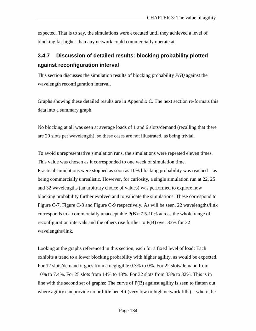
CHAPTER 3: The value of agility
Page 134
expected. That is to say, the simulations were executed until they achieved a level of
blocking far higher than any network could commercially operate at.
3.4.7 Discussion of detailed results: blocking probability plotted against reconfiguration interval
This section discusses the simulation results of blocking probability P(B) against the
wavelength reconfiguration interval.
Graphs showing these detailed results are in Appendix C. The next section re-formats this
data into a summary graph.
No blocking at all was seen at average loads of 1 and 6 slots/demand (recalling that there
are 20 slots per wavelength), so these cases are not illustrated, as being trivial.
To avoid unrepresentative simulation runs, the simulations were repeated eleven times.
This value was chosen as it corresponded to one week of simulation time.
Practical simulations were stopped as soon as 10% blocking probability was reached – as
being commercially unrealistic. However, for curiosity, a single simulation run at 22, 25
and 32 wavelengths (an arbitrary choice of values) was performed to explore how
blocking probability further evolved and to validate the simulations. These correspond to
Figure C-7, Figure C-8 and Figure C-9 respectively. As will be seen, 22 wavelengths/link
corresponds to a commercially unacceptable P(B)=7.5-10% across the whole range of
reconfiguration intervals and the others rise further to P(B) over 33% for 32
wavelengths/link.
Looking at the graphs referenced in this section, each for a fixed level of load: Each
exhibits a trend to a lower blocking probability with higher agility, as would be expected.
For 12 slots/demand it goes from a negligible 0.3% to 0%. For 22 slots/demand from
10% to 7.4%. For 25 slots from 14% to 13%. For 32 slots from 33% to 32%. This is in
line with the second set of graphs: The curve of P(B) against agility is seen to flatten out
where agility can provide no or little benefit (very low or high network fills) – where the

CHAPTER 3: The value of agility
Page 135
t=1 value is non-zero starting (imperceptibly on these graphs) at 16 slots/demand and
rising thereafter.
3.4.8 Results: Blocking probability versus load
As a summary of the detailed results shown in Appendix C, in this section the results are
graphed to illustrate how the blocking probability varies with load.
0
0.05
0.1
0.15
0.2
0.25
0.3
0.35
0.4
0 5 10 15 20 25 30 35
1
2
4
8
16
32
64
128
256
512
1024
Avg. load (slots/demand)
P(B)
Agility (ticks betw
een reallocations)
Figure 3-1 Blocking probability against load
Looking at Figure 3-1, it is no surprise that the blocking probability rises with average
load. At negligible load (up to approximately 10 slots/demand) the blocking probability is
zero for all configurations (there is no scope for blocking). It is interesting that, as soon as
blocking starts to occur, the different reconfiguration intervals spread out in performance
(going to a maximum difference of 5% versus 1% at average load of approximately 19),
then reconverge as the blocking probability gets very high (33% to 32%) – where the
network is near-full and reallocation is of no assistance. That is to say, faster reallocation
provides significant benefit only within a particular load window.

CHAPTER 3: The value of agility
Page 136
0
0.01
0.02
0.03
0.04
0.05
0.06
0 5 10 15 20 25 30 35
1
2
4
8
16
32
64
128
256
512
1024
Avg. load (slots/demand)
P(B)
Agility (ticks between reallocations)
Figure 3-2 Blocking probability against load – focusing on the area of highest gain.
0
0.02
0.04
0.06
0.08
0.1
0.12
0.14
0.16
0.18
0 5 10 15 20 25 30
P(B)
Avg. load (slots/demand)
1
2
4
8
16
32
64
128
256
512
1024
Agility (ticks betw
een reallocations)
Figure 3-3 Re-running the simulations on an RCN from Chapter 2 with matching N/L/α to NSFNet
(but different links) to illustrate there is nothing atypical about the previous results.

CHAPTER 3: The value of agility
Page 137
Figure 3-2 expands the y-axis of the results to show that the results are very clearly
ordered by reconfiguration interval.
To illustrate the maximum benefit this can provide for a carrier with an example
acceptable blocking probability threshold of 1%: The carrier can run their network at
approximately 13 slots/demand with t=1024, or approximately 19 slots/demand with t=1.
To put that differently, greater agility has effectively expanded the capacity of their
network by 46%.
To verify that there is nothing exceptional about NSFnet, the same simulations were re-
run using one of the Randomly Connected Networks from Chapter 2 (diagrams in
Appendix B) with the same number of nodes (14) and links (20) and thus α value as
NSFnet, but with the links arranged differently. After the experience of NSFnet, the
maximum load was capped when P(B) exceeded 10% for all reallocation times, because
that appeared to be a clearly unrealistic operating regime. The results are shown in
Figure 3-3. Unsurprisingly, the results are very similar.
3.4.9 Chapter summary
In this chapter a formal definition of network agility was given and it was shown how
some representative assumptions could make this equivalent to switch agility. The range
of switch agility values in modern technologies was compared and a categorisation by
function – configuration/restoration/protection/OBS/OPS, noting that human
provisioning does appear on this scale – provided.
Then, simulations were performed to determine the network benefit that can be achieved
from increased agility. It was observed that the benefit achieved depended significantly
upon the network load – too low (negligible amounts of blocking) and there was nothing
to improve on; too high and the network achieved inoperable amounts of blocking.
Within the optimal window of load, an improvement of 46% usable network capacity
could be achieved against a maximum acceptable blocking probability of 1% at the cost
of a one thousand-fold increase in network agility – the equivalent of moving into the

CHAPTER 3: The value of agility
Page 138
next technology category faster. This is a significant and worthwhile efficiency
improvement.
However, the likelihood is that the operator’s network will be installed with considerably
more capacity than is required – below the load-level at which agility provides non-
negligible advantage – and therefore spend a significant proportion of its lifetime not
making use of the agility. Further, with geographically large networks the signalling
latency may come to dominate connection setup time (e.g. the round-trip-time of 43ms
across the continental US derived in section 3.1.3) such that switch speeds much faster
than the signalling latency have negligible value.
The operator, when deciding what network agility they require, must therefore choose a
blocking level that they deem acceptable. The maximum blocking level will determine
whether will have their network at the right load-level to take advantage of more-frequent
reallocations, or whether the need for reallocations will be rare enough that a slower and
thus cheaper technology will suffice.
3.5 Chapter references
[Almeida 08] R.C. Almeida, D.R. Campelo, A.V.T Cartaxo, K.M. Guild, H. Waldman,
“Efficient Wavelength Assignment Policy for XPM-Impaired WDM Networks”. IEEE
Communications Letters, Vol 12, Issue 10 (Oct 2008). Pp 791-793.
[Bagula 07] A. B. Bagula, “On Achieving Bandwidth-Aware LSP/λSP
Multiplexing/Separation in Multi-Layer Networks”. IEEE Journal on Selected Areas in
Communications, Vol. 25, No. 5 (June 2007).
[Ballou 02] R.H. Ballou, H. Rahardja, N. Sakai, “Selected country circuity factors for
road travel distance estimation”. Transporatation Research Part A – Policy And Practice,
Vol. 36, Issue 9 (November 2002), pp843-848.

CHAPTER 3: The value of agility
Page 139
[Baroni 98] Stefano Baroni, “Routing and wavelength allocation in WDM optical
networks”. PhD thesis 1998. University College London.
[Cao 07] X. Cao, V. Anand, C. Qiao, “Waveband Switching for Dynamic Traffic
Demands in Multigranular Optical Networks”. IEEE/ACM Transactions on Networking,
Vol. 15, Issue 4 (August 2007), pp 957-968.
[CIA 09] CIA world fact book for the USA, as at January 2009, including land area.
https://www.cia.gov/library/publications/the-world-factbook/geos/us.html
[Cugini 05] F. Cugini, L. Valcarenghi, P. Castoldi, M. Guglielmucci, “Low-cost
resilience schemes for the Optical Ethernet”. Journal of Optical Networking, Vol. 4, Issue
12 (December 2005), pp 829-837.
[Fawaz 08] W. Fawaz, K. Chen, Z. Nakad, C. Abou-Rjeily, “A simple quality-of-service-
based connection setup management approach for optical networks”. IEEE Conference
on Communications (ICC) 2008 (19th-23rd May 2008), China, Vols. 1-13, pp 5349-5353.
[Flood 00] F.A. Flood, “L-band erbium-doped fiber amplifiers”. Optical Fiber
Communication Conference (OFC) 2000 (7th March 2000), Baltimore, Vol. 2, pp 102-
104.
[Friskney 02a] R.Friskney, R. Heath, K. Cordina, “Transient Location for Optical
Networks”. US filing 10/109,199, filed March 2002.
[Gupta 09] H. Gupta, A. Mahanti, V.J. Ribeiro, “Revisiting Coexistence of Poissonity
and Self-Similarity in Internet Traffic”. IEEE Modeling, Analysis and Simulation of
Computer and Telecommunications Systems (MASCOTS) 2009 (21st-23rd September
2009), London, United Kingdom, pp 433-442.

CHAPTER 3: The value of agility
Page 140
[Jeong 05] H.Y. Jeong, S.W. Seo, “Blocking in Wavelength-Routed Optical Networks
With Heterogeneous Traffic”. IEEE Journal On Selected Areas In Communications, Vol.
23, Issue 8 (August 2005), pp 1643-1657.
[Lao 04] R.N. Lao, R. Friskney, R.I.Killey, "Effect of Sparse Wavelength-Conversion
on Network Tolerance to Inaccuracy in Traffic Load Forecasts". European Conference on
Optical Communication (ECOC) 2004 (September 2004), Stockholm.
[Lao 04-2] R.N. Lao, R. Friskney, R.I.Killey, "Investigation of the tolerance of
wavelength-routed optical networks to inaccuracy in traffic load forecasts". Optical Fiber
Communication Conference (OFC) 2005 (6th-11th March 2005), Vol. 4. Paper: OThS4.
[Lao 05] R. N. Lao, R. Friskney, R. I. Killey, "Investigation of the tolerance of
wavelength-routed optical networks to inaccuracy in traffic load forecasts". Journal of
Optical Networking, Vol. 4, Issue 3 (3rd March 2005), pp144-156.
http://www.osa-jon.org/abstract.cfm?URI=JON-4-3-144
[Kantarci 08] B. Kantarci, H.T. Mouftah, S. Oktug, “Arranging shareability dynamically
for the availability-constrained design of optical transport networks”. IEEE Symposium
on Computers and Communications 2008 (6th-9th July 2008), Vols. 1-3, Marrakech,
Morocco, pp 100-105.
[Khazali 08] I. Khazali, R. Vickers, “The Agile All-Photonic Network: Architectures,
algorithms, and protocols”. IEEE Multi-conference on Systems, Signals and Devices
(SSD) 2008 (20th-22nd July 2008), pp 436-440.
[Leland 94] W.E. Leland, M.S Taqqu, W. Willinger, D.V. Wilson, “On the self-similar
nature of Ethernet traffic (extended version)”. IEEE/ACM Transactions on Networking,
Vol. 2, Issue 1 (February 1994), pp 1-15.

CHAPTER 3: The value of agility
Page 141
[Li 06] X. Li, Z. Zhou, M. Hamdi, “Non-violation set scheduling for two-dimensional
optical MEMS switches”. IEEE Communications Letters, Vol. 10, Issue 4 (April 2006),
pp 308-310.
[Ma 03] X. Ma, G.S. Kuo, “Optical Switching Technology Comparison: Optical MEMS
vs. Other Technologies”, IEEE Communications Magazine, Vol. 41, Issue 11 (November
2003), pp S16-S23.
[Ma 08] Y. Ma, “MicroElectroMechanical Systems (MEMS) Based Wavelength-
Selective Building Block in a Transparent Network Architecture”. Communications
Networks and Services Research Conference 2008 (5th-8th May 2008), Halifax, Canada,
pp 326-330.
[Mizukami 04] M. Mizukami, M. Masato, M. Makihara, S. Inagaki, K. Sasakura,
“Development of automated optical fiber cross-connect equipment”. NTT Technical
Review Vol. 2, No. 11 (November 2004), pp63-67.
[Mizukami 05] M. Mizukami, M. Makihara, S. Inagaki, K. Sasakura, “200 × 200
automated optical fiber cross-connect equipment using a fiber-handling robot for optical
cabling systems”. Optical Fiber Communication Conference (OFC) 2005 (6th-11th March
2005), Anaheim, California, Vol. 6, pp 3-5.
[Murakami 08] M. Murakami, T. Seki, K. Oda, “Optical channel power stability in
transparent optical network using large-scale photonic crossconnects and automatic gain
control EDFAs”. International Conference on Transparent Optical Networks (ICTON)
2008 (22nd-26th June), Athens, Greece, Vol. 1, pp 157-160.
[Myers 01] A. Myers, “Architecture for Optical Burst Switching”, MRes Thesis 2001,
University College London.
CHAPTER 3: The value of agility
Page 142
[Pan 08] Y. Pan, Y. Ma, S. Islam, “Electrostatic Torsional Micromirror: Its Active
Control and Applications in Optical Network”. IEEE Conference on Automation Science
and Engineering (CASE) 2008 (23rd-26th August 2008), Arlington, USA, pp 151-156.
[Suzuki 94] S. Suzuki, A. Himeno, Y. Tachikawa, Y. Yamada, “Multichannel optical
wavelength-selective switch with arrayed-waveguide grating multiplexer”. IEEE
Electronics Letters Vol. 30, Issue 13 (23rd June 1994), pp 1091-1092.
[Takahashi 08] K. Takahashi, Y. Kanamori, Y. Kokubun, K. Hane, “A wavelength-
selective add-drop switch using silicon microring resonator with a submicron-comb
electrostatic attenuator”. Optics Express, Vol. 16, Issue 19 (15th
[Tellabs 09] Tellabs white paper, “Beyond Five Nines: The New Age of “Uber
Reliability”.
September 2008), pp.
14421-14428.
http://www.tellabs.com/resources/papers/tlab_uberreliability.pdf. February
2009.
[Terui 91] H. Terui, T. Kominato, M. Kobayashi, “Lossless 1×4 laser diode optical gate
switch”. Journal Of Lightwave Technology, Vol. 9, Issue 11(November 1991), pp 1518-
1522.
[Times 03] Times Books Group Ltd., “The Times Concise Atlas Of The World”, Eighth
Edition, Printed 2003.
[Zapata-Begheli 08] A. Zapata-Beghelli, P. Bayvel, “Dynamic Versus Static
Wavelength-Routed Optical Networks”. Journal of Lightwave Technology, Vol. 26, No.
20 (15th October 2008). Pp3403-3415.

CHAPTER 4: Path viability and its effect on photonic control planes
Page 143
Chapter 4 Path viability and its effect on photonic control planes
In the previous chapter, conditions were discussed under which greater photonic network
agility could provide value to an operator in terms of new service types (requiring
particular setup/restoration time bounds) or of network bandwidth efficiency –
accommodating more traffic on the same network, or the same traffic with a smaller
network. It was noted that it is possible to set up wavelength-paths in a photonic path that
are not optically viable (i.e. that do not achieve an acceptable (according to operator
policy) received Bit Error Rate1
First a formal definition of optical viability is provided for both the A-WRON and WPS
cases discussed in this thesis, then alternative methods of pre-determining viability are
reviewed, a new calculation of the error involved in prediction based on live impairment
) and are thus not usable. It was assumed that it was
possible to pre-determine whether a path was viable and thus there would never be the
attempt made to set up a non-viable path. Because of this possibility of non-viability, any
kind of photonic provisioning system/control plane will need to pre-determine the
viability of a path before it is set up, or handle the case where a provisioned path proves
to be non-viable by some technique.
The purpose of this chapter is to describe and compare these alternative approaches to
viability calculation and to determine their implications on the use of photonic control
planes.
Work published from 2002-2004 relating to ‘traditional’ IMDD (intensity-modulated
direct detection) is described. Since then, phase-modulation/coherent reception and DSP
technology has offered a dramatic step forward in bitrate and impairment tolerance. A
section is provided discussing the implications of this on the earlier work.
1 A formal definition of viability is given later in this chapter.

CHAPTER 4: Path viability and its effect on photonic control planes
Page 144
measurement is given for an IMDD system. Finally, the implications of the limitations
discovered on usage of a photonic control plane are discussed.
4.1 Definition of optical viability and optical viability engine (OVE)
The ‘health’ of a wavelength-path is measured by the Bit Error Rate (BER). Each
network operator will have a policy on the worst BER they will accept for a newly-
provisioned wavelength-path. The target is commonly set in terms of the newly-
provisioned BER - it is assumed equipment performance reduces over time.
BER is usually measured after all processing such as Forward Error Correction (FEC) has
been applied, as this is the error rate that the service data is subject to. This target can
then be common across all transmission media in terms of the requirements of the service
application. Some operators set their viability targets in terms of the pre-FEC BER
because lower error levels (that the FEC can remove from the service data) will be
apparent. However, as the ultimate goal is to deliver service data end-to-end across the
network with a particular BER, measuring viability pre-FEC would mean that different
targets would be required according to the strength of the FEC used, so this is only
appropriate within a set of similar transponders.
Definition: An optically viable path is one that meets or is better than (experiences less
errors than) the operator’s target BER.
This definition (routes suitable “for path selection”) is shared with the IETF’s draft
standards work in this area (see reference [Wson-impairments]). Common published
standards for acceptable post-FEC BERs are given in Chapter 1. For transmission of
>1Gbps, these provide a target of 1 error in 1012
Direct measurement of BER would take a long time by machine standards – 10
bits received.
12 bits at
40Gbps takes 25 seconds. Methods for measuring the optical Q-factor include (after
CHAPTER 4: Path viability and its effect on photonic control planes
Page 145
[Mishra 10], for example) allowing the BER to be extrapolated by determining the edges
of the optical eye.
For use in the comparison of routing techniques that follows, the further concept of
Optical Viability Engine is required:
Definition: An Optical Viability Engine (OVE) is a software component that will
indicate whether a given wavelength-path will be viable. [Peeters 04]
In standards (IETF) terms, optical viability (or “impairment validation” as the IETF calls
it) is discussed in the reference [Wson-impairments] and commonly outsourced from the
control plane to a “Path Computation Element” (PCE) functionality introduced in
[RFC4655]. A photonic PCE is defined by the IETF as including the functionality of an
OVE. Further discussion is in section 1.8.
4.1.1 Why may a wavelength-path be non-viable?
Unlike most other forms of data communications, the advantages of photonic networks
(described in Chapter 1) come when no electronic processing at intermediate nodes is
performed. Electronic processing gives ‘3R’ (re-amplification, re-timing, re-shaping)
regeneration implicitly, but only amplification is usually present in all-optical systems, so
signal impairments accumulate at each hop. Thus, transitivity is lost – if A can reach B
and B can reach C, then A may very well not be able to reach C if the longer path reduces
the signal quality below a usable level. Some examples of impairments that accumulate
(not necessarily additively) are noise and polarization mode dispersion (PMD),
Further complicating the problem, some parameters need to be within an optimal window
rather than minimised, e.g. chromatic dispersion (for systems without electronic
dispersion compensation, e.g. most existing installed systems). As an example, if A-B is
non-viable due to excess positive dispersion and B-C is non-viable due to excess negative
dispersion, on route A-B-C the dispersion may cancel out sufficiently to result in a viable
CHAPTER 4: Path viability and its effect on photonic control planes
Page 146
path. An example of this would be where A-B was a long series of uncompensated fibre
links and B-C was a short fibre link with a large dispersion compensation module.
Another form of non-viability is fundamental incompatibility – e.g. if link A-B was
provided by vendor X, link B-C was provided by vendor Y and vendors X and Y used
different wavelength grids, it might not be possible to route a wavelength via A-B-C
regardless of the impairments on these links. Such fundamental incompatibility is
declared out of scope of this chapter as it is not a common practical problem: photonic
networks are usually designed to have line equipment only from a single vendor with
regeneration before hand-off to another line system.
The impairments considered in this chapter are of two forms, linear impairments such
as loss and dispersion and non-linear effects such as four-wave mixing (FWM), cross-
phase modulation (XPM – the effects of which are described in depth in [Thiele 00]),
cross-polarisation modulation (XpolM), self-phase modulation (SPM). Other fibre
nonlinear impairments exist (e.g. stimulated Raman scattering (SRS) and stimulated
Brillouin scattering (SBS)) but these are negligible in current systems that compensate for
them. A comprehensive treatment of all of these effects and noise sources such as
amplified spontaneous emissions (ASE) can be found in [Agrawal 95] and [Agrawal 97].
The dispersion map is the sequence of fibre segments and network elements with
chromatic dispersion effects, and the size and sign of dispersion of each segment/element.
An example earlier in this section referenced the simple net sum of the positive and
negative dispersion along a wavelength-path. However, the precise ordering of the
elements within the map may increase or decrease other effects notably SPM and XPM as
further discussed in [Thiele 00]. Other significant factors that likewise have an effect on
the impairments that will be experienced are other channels’ spacing, power and
modulation format.
CHAPTER 4: Path viability and its effect on photonic control planes
Page 147
4.1.2 Control plane functions that require viability information, and the requirements this places upon the OVE
Any control plane function that involves provisioning a wavelength-path along a new or
modified route will require a viability check: provisioning of new connections,
modification of existing paths, protection or restoration around faults.
Below are listed how these set requirements on the system provisioning speed (i.e.
network agility, the subject of the previous chapter), and thus indirectly on the
operational speed of the OVE:
- Human-triggered provisioning needs ideally to complete within the span of
human patience on a GUI – perhaps a few seconds.
- Machine-triggered provisioning, where an example would be a higher layer
having gone past a congestion threshold, needs to dial up some extra bandwidth.
This provides no particular time target, but the upper bound on connection setup
speed will determine how late the upper layer can leave signalling for additional
bandwidth and thus reducing the upper bound will result in greater higher-layer
efficiency.
- Protection switching will require a bounded time. The well-known 50ms target (a
common expectation codified in standards such as [GR-253-Core]) would be
required for some paths. A US regulatory target described in the previous chapter
is 10 seconds. 50ms is commonly delivered by using a pre-established backup
path ([GR-253-Core] suggests this approach). If the photonic system is agile
enough to calculate, validate and establish a wavelength-path within 50ms then
pre-establishing the backup path may not be required – increasing network
efficiency by not requiring more than half of the capacity of the network to lie
permanently idle in the longer protection paths.
In addition to those control plane functions that use viability information, a control plane
implies distributed intelligence, that path setup can be initiated from multiple points in
the network – e.g. from any node. Section 4.2.4.1 describes later a method of extracting
this information from the network and distributing it to all the nodes that will need it for

CHAPTER 4: Path viability and its effect on photonic control planes
Page 148
their route computation. [Azodolmolky 09] provides more detail on a potential protocol
infrastructure for distributing the information.
4.1.3 Opportunities for viability calculation optimisation in agile control planes versus static provisioned systems
Commonly today, wavelengths are provisioned such that they may be kept operating as
on the same route and equipment for an estimated lifetime of 20 years, or a similarly
lengthy period. This is associated with an unwillingness to disrupt a revenue-earning
service once it is installed, and an existing slow, expensive and error-prone human-based
re-routing process.
An agile photonic network with shorter wavelength lifespans has an advantage in terms
of being able to ignore or reduce link budget margins for factors related to long lifespan
(what [Azodolmolky 09] calls time-varying impairments). These factors are:
- Additional fibre loss later in life due to breakages fixed by splicing. The
breakages are mainly caused by civil works activities accidentally digging
through the fibres.
- Amplifiers2
- Receivers ageing and becoming less sensitive.
ageing and increasing their noise figure.
- The ability to use current measured performance values (where present) versus
component specifications. This option is discussed in much more detail in the
measure-and-predict section later.
Examples of where at least some wavelength-paths may have predictably shorter
lifespans are:
2 It is assumed that amplifiers are EDFA in this chapter, as that reflects the experimental work that was
done. However, the work equally applies if they are Raman amplifiers additionally or instead of EDFAs
because it is the net effect of a span that is being considered. This statement assumes that measurement
points are not further impaired by the Raman pump light. For the specify-and-predict approach it assumes
that the effect of the Raman pump is specified as well as for an EDFA which may not be true if the
transmission fibre is not well characterised – e.g. the Raman is an upgrade on old poorly-specified fibre.

CHAPTER 4: Path viability and its effect on photonic control planes
Page 149
- Where a service is pre-booked for a stated finite duration, rather than the
expectation that it will serve until cancelled. Currently this is not general practice
and so is only seen for rare special events (e.g. the Olympics). However, it is not a
significant restructuring of the customer/carrier relationship as prices would often
be adjusted/renegotiated every few years anyway.
- Where a particular service type is defined to have a maximum lifetime. For
example, if the ability to dial-up wavelengths were provided to users with large
but short-term requirements (e.g. virtual machine migration between data centres,
downloading of large experimental data-sets) then their contract could state that
each path would automatically be terminated after 24 hours in the unlikely case its
termination had not already been requested by the customer.
- Where the carrier expects to perform regular network defragmentation (re-
optimisation) of their wavelength-routes. A major North American carrier
currently has a policy of defragmenting their SONET network every 6 months due
to the exceptional growth they are experiencing, so it may be assumed that as
agile wavelength networks develop it may be seen with wavelength-paths too.
- Where a wavelength-path is provisioned temporarily as a restoration route and the
operator has a policy of fixing the original route and reverting the traffic to it, so
the expected requirement for the restoration path is just the worst-case repair time.
This is common practice because the original path would have been chosen as
part of an overall optimal path layout, or because it was the least-cost path
available. Further/alternatively, the restoration path may have higher latency (e.g.
due to more fibre-kilometres traversed) which the end-customer could detect and
complain.
Reduced link budget margins mean that more wavelength-paths are viable without
regeneration, notably longer wavelength paths. This will reduce the number of
regenerators required to operate a network, and thus the network cost. Or conversely, for
a fixed set of regenerators, allow more network traffic to be accommodated.

CHAPTER 4: Path viability and its effect on photonic control planes
Page 150
Control planes still need to leave some margins for factors such as PMD that can change
faster than a wavelength is likely to persist. For example, a submarine fibre (perhaps the
most stable environment a cable could be in) was found to change its PMD value by
>0.25ps over 70% of 15s intervals during daytime in [Zhang 07]
Required operating margin and the different approaches to it are factors that are often not
considered in the networking literature e.g. [Azodolmolky 09] describes the EU research
network DICONET which is very similar to the agile WRONs described in this thesis. He
states that his Q factor estimator predicts performance based on the currently-provisioned
wavelengths before deciding whether to provision new wavelength X. However, if
further wavelengths are added, these will result in greater impairment to X (e.g. via cross-
phase/cross-polarisation modulation (XPM/XpolM) or four-wave mixing (FWM)). Other
system changes may similarly result in increased impairment (e.g. power re-balancing
due to wavelength adds/deletes elsewhere). If the operating margin of X is not adequate
to allow for this increased impairment, it will then fail in operation before its design
lifetime has expired. As mentioned, on a longer timescale, effects such as fibre breaks
and re-splicing may similarly cause an operating wavelength to fail. Therefore, required
margin (and its relationship to anticipated wavelength duration of being in-service) is a
key factor in viability.
As this work does not assume any particular control plane approach, it is equally
applicable to Grid-type control systems which dial up both IT and networking capacity as
described, to pick a recent example among many, [Grosso 09]. This paper is chosen
particularly because it uses the Nortel/Ciena photonic system used as an example
throughout this thesis.
4.1.4 Viability and WPS
Wavelength path sharing is described in Chapter 2. In terms of viability, each transmitter-
receiver pair must be separately considered, i.e. each demand service along a given
logical path. The example in section 4.1.1 is directly translatable to WPS as it shows
where in a viable path A-B-C, the sub-paths A-B and B-C may be non-viable.

CHAPTER 4: Path viability and its effect on photonic control planes
Page 151
However, in terms of determining whether a particular transmitter-receiver pair is viable,
WPS is using precisely the same technology as A-WRON and so the viability calculation
problem is the same – applied for each of the transmitter/receiver pairs within a planned
logical path. Therefore this chapter discusses only the A-WRON case without loss of
generality.
4.2 Comparison of control plane and provisioning approaches to viability calculation
This section reviews the different approaches that control planes/provisioning systems
can take to calculating viability and compares them according to the criteria given next. It
is a write-up of concepts co-published in [Peeters 04].
4.2.1 Criteria for comparing viability approaches
The following parameters are used to compare the different techniques:
- Speed of response of viability calculation. At the time of writing, the most
accurate technique that Ciena has to predict performance is the split-step Fourier
propagation simulation (a recent approach including a review of this area is
provided in [He 10]), which takes over 24 hours to execute for a single
wavelength route. This is not compatible with restoration targets of 10 seconds or
50 milliseconds as set out earlier in the chapter, but could be used for pre-planned
activities.
- Accuracy of result - percentage of false positives/negatives. False positives may
cause the need to tear-down and retry the connection, causing additional setup
latency. False positives within the allocated margins for PMD etc. will cause
unreliability – wavelength-paths that appear to be viable but sometimes (e.g. in
adverse polarization conditions brought on by strong winds on fibres) fail
unexpectedly. False negatives will reduce network efficiency by rejecting optimal
paths. [Azodolmolky 09] considers this another form of blocking. An alternative
approach would be to allow a retry.
CHAPTER 4: Path viability and its effect on photonic control planes
Page 152
- Constraints on network design. These and their impacts are discussed in the
individual sections.
- Efficiency at minimizing OEO regeneration.
The methods in the next sections fit into three broad categories:
- Apply planning constraints such that viability calculations are not required for
new paths.
- Run sophisticated viability calculations.
- “Try it and see”. Actually provision a path and measure performance at the
receiver to determine whether it is viable.
4.2.2 Optical islands
The physical topology is divided up into ‘islands’. Between the islands all traffic is
regenerated. Thus, each island is a separate photonic domain. The islands are engineered
such that any ‘sensible’ (e.g. “up to 6 hops” or “within 2 hops of the shortest path”)
photonic path is viable [Saleh 00].
Where there are natural boundaries already between small (all ‘reasonable’ paths viable)
network domains, e.g. between photonics rings with dissimilar types of optical systems
(e.g. different vendors), then the optical islands approach is the obvious choice.
The advantage of this method is that viability calculation is not required per-path and so
causes no calculation delay. Further, any reasonable routing algorithm may be used,
provided it is compatible with the planning rule used. This method is therefore commonly
used (usually implicitly and without discussion) for systems like OPS/OBS, where there
is no time for attempting a second path.
Where a domain has only partial reachability, but the operational simplicity of islands is
desired, the domain may be transformable into an island by using longer reach/more
expensive transponders.

CHAPTER 4: Path viability and its effect on photonic control planes
Page 153
The disadvantages of this method are that:
- Wavelengths travelling very short distances that happen to cross an island
boundary will be regenerated when these paths would be viable without
regeneration – i.e. unnecessary cost. This example is equivalent to an inaccurate
viability prediction.
- It is a significant network design constraint to use only limited-size (determined
by reachability) islands.
4.2.3 Network trial and error
The path is provisioned and the BER of that path is measured. If the BER is satisfactory
and the system determines that the path will stay viable for its expected lifetime (see
below), the path is accepted for traffic. If the path is not accepted, an alternative path may
be tried – algorithms discussed below.
Even if the wavelength-path immediately achieves adequate BER, it does not mean it will
continue to be viable. Time-varying impairments such as PMD [Savory 06] may later
increase. Therefore, a margin above the target BER will be required, calculated from the
known statistics of the impairments, the policy of the operator on acceptable risk, and the
duration for which the path can be measured before a decision is required. The reader is
referred back to section 4.1.1 which discusses how long a direct BER measurement may
take, although a pre-FEC BER measurement would normally be used as this will get a
more rapid result. Further, depending upon the acceptance policy of the operator, the path
may need to dry run for longer periods to e.g. experience day/night changes in
performance. A trade-off must be struck between network bandwidth efficiency
(minimising margins) and setup speed (using larger margins to compensate for lack of
knowledge of the statistics of variable impairments encountered rather than longer
measurement periods).
This approach is very well-suited to a system where:
- routing is done via a least-cost path;
- the dominant impairment is simply additive (such as noise);

CHAPTER 4: Path viability and its effect on photonic control planes
Page 154
- the noise added by each link is proportional to its routing algorithm link cost;
or otherwise such that the least-cost path is also an approximation to the least-impaired
path. Given this assumption, the first path tried is likely to succeed. In contrast, if the first
few tries fail, it is unlikely that any path will succeed and the connection can sensibly be
rejected.
Contrariwise, if the routing algorithm is unlikely to try the least-impaired path, then the
system must budget for several failed attempts before one succeeds.
Because this approach makes use of actual measured end-to-end performance on the
route to be used, it can make use of unexpectedly good performance (e.g. equipment
outperforming its specifications) where the greater margins of other approaches may
cause them to regenerate unnecessarily. It is the only method usable when photonic
performance cannot be modelled effectively in advance.
It is unattractive where any of the following conditions hold:
- A large number of ‘sensible’ routes will be non-viable, causing it to be very
cumbersome - trying lots of useless routes.
o E.g. long-distance networks where at least one or two steps of
regeneration will be required.
o It would need to be combined with a simple regenerator-selection, which
would then need its own viability calculation approach.
- Setting up paths can only be done slowly and carefully to avoid disruption of
other wavelengths and/or has a cost of some sort – e.g. potentially requiring
equipment to be deployed, requiring some manual intervention, risking
interruption of service of other wavelengths.
- The margin for variability has to be high - e.g. the network is prone to large
day/night performance variations, PMD, component ageing margin. Some of
these may be removed by operating the path for a long period (e.g. a few weeks)
and averaging the performance before a pass/fail report is given. Ageing margin
may be adjusted if an expected hold-time is known for the path. Such multi-week
CHAPTER 4: Path viability and its effect on photonic control planes
Page 155
measurement periods may not be compatible with the targets of the operator for
agility/time to revenue. They are also not compatible with needing to try several
routes to find a suitable one.
- Regenerators are likely to be required along the path and the routing algorithm
must determine where they are to be used – in the most naïve implementation this
algorithm would have to try every possible unregenerated route before trying
every possible one-regenerator route, then every possible two-regenerator route
and so on. Heuristic enhancements would be possible e.g. after two failed un-
regenerated path attempts, add the regenerator topologically nearest to the shortest
paths.
- Already-operating wavelengths have such a small margin that each provisioning
act carries a non-negligible risk of disrupting service.
In terms of the parameters for evaluation:
- Speed of viability “calculation” in this case is the sum of the number of failed
path setups plus the measurement times required.
- Accuracy of result: A trade-off with measurement time, as discussed above.
- Constraint of network design: No constraints.
- Efficiency in minimizing OEO regeneration: This simplest version does not
address the problem at all. It will use an unregenerated path where it can be
viable.
4.2.4 Measure-and-predict
During the operation of the network, each of its links are characterised in terms of
impairments by direct measurement - a possible implementation is provided below. Then,
when a new route request is received, a viability prediction is made on the basis of this
information. Example equations for doing this are given in section 4.3
Definition: A probe wavelength-path is one not used for end-user data, and is solely
established to enable characterisation of the segments of the network it travels through.

CHAPTER 4: Path viability and its effect on photonic control planes
Page 156
In order to get information before a link is used, probe wavelength-paths may be set up.
Probe wavelength-paths may use idle regenerators as transmission sources.
Alternatively/additionally, probe wavelength-paths may use ROADMs (reconfigurable
optical add-drop multiplexers) to split existing wavelength-paths (probe or user) into their
original path and one or more probe paths, although this is restrictive in that the probes
will all be at the same wavelength as the original. Once the network has at least one
traffic-carrying wavelength on each link, there is no further use for probe wavelength-
paths – i.e. there is no long-term requirement for probing equipment.
While the network is in operation, monitoring can continue on traffic-carrying and probe
wavelength-paths to detect performance drifts over time.
In terms of the parameters for evaluation:
- Speed of viability calculation:
- Accuracy of results: Section 4.3 is dedicated to this question.
- Constraint of network design: No constraints. Requirement for enough hardware
(spare transponders) at initial deployment for network to characterise itself before
use, although this requirement goes away when network is fully in use (all links
have at least one wavelength). Requirement for monitoring equipment at each
node which has cost. The Ciena system has an Optical Spectrum Analyser (OSA)
- as part of its optical performance monitor (OPM) function - present at every
ROADM site anyway as part of the wavelength power-control/gain-flattening
control system, so this can be used at no extra cost by a control plane.
- Efficiency in minimizing OEO regeneration: Makes full use of system reach,
except due to false-negatives due to inaccuracy on viability.
This technique is similar to the drafts currently proposed in the IETF standards body
[Bernstein 10], [wson-impairments], and by the ITU in G.680. However, these standards
currently only describe how to model the impairments of each component and calculate
cumulative impairments of all the different types (noise, PMD, polarization-dependent

CHAPTER 4: Path viability and its effect on photonic control planes
Page 157
loss (PDL) etc.) without the required final step of an actual BER prediction such as is
provided in the next section.
4.2.4.1 Example measure-and-predict system
The example system was built as a test-bed at the Kao-Hockham laboratories (now
closed) in Nortel Harlow. A more analytical presentation and an error analysis are
performed in section 4.3.
This section uses the concept of Optical Signal-to-Noise Ratio (OSNR). This is simply
the ratio of the average signal optical power to the average signal noise power [from
Agrawal 97]:
=
N
S
PP
OSNR 10log10 (4-1)
Where OSNR here is given in dB.
PS is the signal power (in any units)
PN is the noise power (in units to match PS
An example of a measure-and-predict system is described in this section. This is chosen
as it is evaluated further in section
).
Practically, this measurement is made over a given bandwidth Δf as the receiver will only
pick up noise (or indeed signal) over a finite bandwidth.
4.3. Figure 4-1 shows the configuration of the system.
At each photonic cross-connect or ROADM, each wavelength is periodically measured as
it enters and leaves the transmission fibre. Two measurements are performed. The first
measurement is an Optical Spectrum Analyser (OSA). This is used to measure change in
optical signal to noise ratio across the link (Δ-OSNR) – from which can be extracted the
impairment due to optical noise added by this link. The second measurement is a Q
monitor. This measures the overall differential impairment across the link. Subtracting
the noise-based impairment from the total impairment across the link gives the distortion
impairment – described in the figure as Δ-distortion. See section 4.3 for a mathematical

CHAPTER 4: Path viability and its effect on photonic control planes
Page 158
treatment of this, and path performance based on this information. For cost reasons, the
OSA and Q monitor are shared between all of the wavelengths at a site and a photonic
switch is used to apply them to all of the input/output ports of that site in turn. A passive
optical tap from each line means that such monitoring is non-intrusive.
It is significant that in terms of OSNR measurement, it is the OSNR contribution of the
link being measured rather than absolute OSNR values. This is because OSNR is defined
as the ratio of the signal to the noise within that wavelength. However, the noise within
the wavelength cannot be separated by an OSA (it measures what power is there, not
where it comes from); therefore the OSA measures the noise to either side of the
wavelength signal and extrapolates the noise floor under the signal. When going through
wavelength-separating filters, the noise floor between wavelengths will be changed –
“noise floor shaping”. Therefore the absolute OSNR measurements will be invalid.
Performance monitoring integration
PXC
0 1 2 3 4 5 6 7 8 9 1
- - - 0 0. 0. 0. Q OSNR
Optical Data - base
GMPLS OSPF
PM
∆ - OSNR ∆ - Distortion
PXC
0 1 2 3 4 5 6 7 8 9 1
0
- - - 0 0. 0. 0. Q OSNR
Optical Data - base
GMPLS OSPF
PM
∆ - OSNR ∆ - Distortion
Physical layer
Performance Monitoring
layer
Q, OSNR
Control layer Optical Metrics
Figure 4-1 Passive taps from the optical cross-connects feeding into a shared performance monitor (one per
node) giving Q and OSNR measurements. Reproduced from [Friskney02a] with permission.

CHAPTER 4: Path viability and its effect on photonic control planes
Page 159
However, measurements are taken at wavelength-multiplexed points – just before the first
amplifier and just after the last amplifier. Therefore, the comparison of these two
measurements is still valid, even if the absolute values are not.
The distortion values measured will include any inter-channel effects such as XPM.
However they will not capture how those impairments will change as more channels are
added later. A margin must be added to compensate for that depending upon the channels
which can be added from the current fill level to the maximum fill level anticipated
within the period that the wavelength-path will be used.
4.2.5 Specify and predict
This method takes the manufacturer specifications of all of the equipment in the path and
then predicts the end-to-end wavelength performance. Some options for path
performance prediction:
- Full split-step propagation simulation (such as discussed for example in [He 10])
- A simple noise + impairment-estimate model such as provided in 4.3.
- Some hybrid of the above.
The photonic planning tools produced by Ciena use an accelerated split-step Fourier
propagation simulation by using a proprietary approach of pre-calculated lookup tables
where possible.
Advantages of specify-and-predict over measure-and-predict:
- More accurate measuring equipment is available in a factory than in an
operational network and more insightful characterisation can be performed. This
assumes such per-unit factory calibration data can be stored in and read from the
equipment. Passive equipment (DCMs, fibre) may not have a mechanism to report
such characterisation data.
- No additional measurement equipment required in the network.
- Fixed information over the lifetime of the network so impairments can be
precalculated if required.

CHAPTER 4: Path viability and its effect on photonic control planes
Page 160
Disadvantages of specify-and-predict over measure-and-predict:
- If there is significant performance variation between instances of the same
product, the specification data will have to incorporate this – unless per-unit
calibration data is included as discussed above.
- Performance data will have to include ageing margin for the product’s lifetime.
4.2.6 Comparison table of viability methods
Table 4-1 provides a comparison of the viability methods listed in previous sections,
evaluated against the criteria provided in section 4.2.1.
Optical
Islands
Trial & error Measure &
predict
Specify &
predict
Speed of
response of
OVE
No
calculation
required.
N * Wavelength turn-
up and measurement
time.
Negligible
(*)
Negligible (*)
Additional
margin (and
thus utilisation
inefficiency)
required (**)
Built in at
planning
stage
For ageing only. For ageing
only
For ageing +
component
variation
tolerance.
Additional
measurement
equipment
None None OSA/Q
monitor per
switching
site.
None
Network design
constraints
Requires
islands
No constraints. No
constraints.
No constraints.
Suitability for
fast switching
such as
WROBS
Yes Requirement for
multiple attempts may
result in unacceptable
delay.
Yes Yes
Table 4-1 Summary of viability assessment methods measured by comparison parameters

CHAPTER 4: Path viability and its effect on photonic control planes
Page 161
(*) –This assumes that both measure & predict and specify & predict use the simple
impairment model described in the next section. In our experiments this model took an
imperceptible time to execute compared to the seconds required by the photonic switch.
Without having measured it, this only allows the characterisation of << 1 second.
(**) – Margins for PDL and similar fast-moving variations are not noted, as they are
common to all options.
4.2.7 Conclusions of comparison of viability methods
At present, A-WRON systems tend to assume viability e.g. [Um 08][Tinter 08] (and
trivially, as it is PON-based [Segarra 06]), which limits their applicability to small
networks, or networks with an optical islands design approach.
Presently, one of the limiting factors in WROBS is the worst-case path set-up time.
[Um 08] [Zapata 03][Zapata 04] Therefore, increasing this by one or several additional
path set-up times with the trial-and-error method seems unattractive – it will increase
intrinsic network latency, thereby decreasing the buffer fill to trigger a burst, decreasing
network efficiency.
While the measure/specify & predict methods would require more complex routing
algorithms in WROBS to take account of the possibility of non-viability, the additional
computation time should still be negligible (with the assumptions stated in section 4.2.6)
by comparison with the path setup delay. [Guild 06] does a similarly elaborate calculation
for OBS/OPS.
Theoretically, measure & predict should out-perform specify & predict because there is
no need to include further margin for component unit variation (although recording of
per-unit factory calibration data may eliminate this issue for specify & predict as
discussed above), and with knowledge of the target wavelength hold-time, there can be a
significant reduction in ageing margin.

CHAPTER 4: Path viability and its effect on photonic control planes
Page 162
Considering how the additional cost of the Q monitor and OSA might decrease over time
in the all-optical future:
• There will always be additional components versus the other viability options and
so have non-zero extra cost.
• Only one Q monitor/OSA is required/cross-connect site. Extrapolation may be
possible if the network is 100% populated, although the accuracy impact of this
sub-population is not considered in the calculations below.
• Speed of measurement is not critical, as this measurement is not part of the turn-
up workflow.
• Alternative approaches for deriving OSNR and Q are arriving via developments
such as [Ye 07] and his multi-Gaussian curve-fitting to histograms of signal
levels. [Skoog 06] believes that such things can be both cost-effective and
revealing. These are samples from a huge body of work on performance
characterisation. The purpose of this comparison is to discuss the general case of
the different approaches and so review of that field is out of scope.
Where a network may be segmented into optical islands without adding additional
regenerators, this approach is simplest of those considered and should be used. For the
general case of networks, assuming that in the all-optical future it becomes affordable to
have a compact OSAs and Q monitor at a high proportion of the nodes, measure-and-
predict should theoretically produce the best performance. The next section considers
what this performance could be and the influence of the accuracy of the measurement
equipment on it.
4.3 Accuracy of On-Off Keying (OOK) measure-and-predict algorithm
A summary version of this section was published as [Friskney 02] and in more detail as
internal report [Friskney 02a]. Where elements are Copyright Ciena from that internal
report, they are reproduced with permission.

CHAPTER 4: Path viability and its effect on photonic control planes
Page 163
In this section equations behind the measure-and-predict algorithm are derived and then
novel error propagation calculations are performed on them. A
simplification/instantiation of this is offered based on current measurement equipment,
showing that current accuracy is very poor, and setting new targets for future
measurement equipment.
The objective of this section is to establish how accurate these calculations are given
known measurement equipment capabilities. It is emphasised that the contribution of this
section is that error analysis rather than presentation of this particular measure-and-
predict framework. The framework essentially models nonlinear distortion as horizontal
eye-closure, assuming that vertical eye-closure comes predominantly from noise.
However, [Thiele 00] shows that the effects of XPM are seen mainly through vertical
eye-closure, with negligible timing jitter (horizontal eye-closure). This was not known to
the experimenters at the time, but better-reflects modern systems with many wavelengths
(XPM pumps), high bitrates and non-dispersion-compensated systems (so causing the
interference time of a pump data-bit A with a signal bit B to be lower than with older
low-rate/fully-span-compensated line systems).
4.3.1 Calculating a link noise metric
This metric has physical significance in that it measures the amount of noise power or
distortion that will be experienced by a signal traversing this link.
The link metric is derived along similar lines to that in [G.680] (the ITU standard on
calculation of an impairment metric) “Impact of cascaded ONEs (Optical Network
Elements) on line system OSNR”. This standard does not bring together the impairments
into a predicted BER or perform an error analysis on the result. See for example [Qin 10]
who does predict a BER but does not perform an error calculation.
At each tap, signal power and OSNR is measured. The node at the downstream end of the
link (remote) passes these measurements to the node at the upstream end (local) of the
link where they are combined as follows (paying careful attention to the units used):

CHAPTER 4: Path viability and its effect on photonic control planes
Page 164
Losslink = PowerLocal_dBm – Power (4-2)
Remote_dBm
This is often negative, indicating a net gain over the course of the link due to
amplification.
First, the absolute noise power is measured at the start and end of the link – note that no
wavelength multiplexers or demultiplexers must be between these two points or noise-
floor shaping effects will cause error in the results, assuming that the usual interpolation-
based OSNR measurement equipment is used. The loss adjustment on the local
measurement is such that this is the noise as would be seen at the remote end, if no noise
were added in this link.
linearLocallinearLink
mWLocalmWLocal OSNRLoss
PowerNoise
__
__ =
(4-3)
linearmote
mWmotemWmote OSNR
PowerNoise
_Re
_Re_Re =
(4-4)
A simple subtraction yields the noise power attributable to this link, which is propagated
as a property of the link l: Noisel = NoiseRemote_mW – Noise
4.3.2 Using link noise metrics for path calculations
Local_mW.
In the final path calculations, the total anticipated noise power for a given path p is:
∑ ∏∈∈
=pl
lSkk
lmWPath Loss
NoiseNoise
)(
_
(4-5)
where S(l) is the set of links in the path strictly succeeding l, i.e. all those links between it
and the destination, from the perspective of following the path. In incremental path
calculations (e.g. Dijkstra), this has the convenient feature that for each new link added, a
CHAPTER 4: Path viability and its effect on photonic control planes
Page 165
running path noise total can be kept by dividing the current total by the new link loss,
then adding the link noise power contribution:
))(()()(
__
)(_
_
lSkpklPk
LossNoisepowerLaunch
LossNoisepowerLaunchOSNR
pl lPkkl
mW
pllmWPath
mWlinearPath
∉∩∈=∈
==∑ ∏∏∈ ∈∈
(4-6)
Again, for incremental path calculations it is useful to keep a record of a running path
OSNR. This equation shows that by storing the denominator and cumulative loss, the
OSNR for a new link z can be calculated readily with four operations:
1) Update the cumulative loss with the loss of the new link z.
2) Multiply the noise from link z by the new cumulative loss.
3) Add the noise factor from 2) to the cumulative denominator.
4) Divide launch power by the new cumulative denominator.
In fact, the actual measurable OSNR will be:
OSNRMeasurable=1/(NoiseInitial/Launch_powermW+1/OSNRPath_linear), where NoiseInitial is
the measured noise floor at the ingress to the managed domain, e.g. the input of the first
PXC. OSNRPath_linear
4.3.3 Error propagation in noise calculations
is useful only for path optimisation calculations, i.e. where relative
numbers are all that matter.
The standard error propagation formula to find δA (error on parameter A) where A=B+C,
(δA)2=(δB)2+(δC)2
is used in this section. From this, the error in per-link noise figure is:
( ) ( )[ ]
+
+
+
+
+
=
+
+
+
+
=
+
=−=
2Re
2222
2
2
Re
Re
2
Re
Re2Re
2222
2
Re
Re
2
Re
Re2Re
22
Re
ReRe
1
)(
moteLocalLocal
Local
Local
LocalLocal
mote
mote
mote
motemote
Local
Local
Local
LocalLocal
mote
mote
mote
motemote
LinkLocal
Local
mote
moteLocalmotelink
PowerPowerLossOSNR
OSNRPowerPowerNoise
OSNROSNR
PowerPowerNoise
LossLoss
OSNROSNR
PowerPowerNoise
OSNROSNR
PowerPowerNoise
LossOSNRPower
OSNRPowerNoiseNoiseNoise
δδδδ
δδ
δδδ
δδ
δδδδ
(4-7)

CHAPTER 4: Path viability and its effect on photonic control planes
Page 166
With algebraic shorthand of:
∑ ∏∈ ∈
+=pl lPk
klInitial LossNoiseNoiseZ)(
and: 2
__
=
mW
mW
powerLaunchpowerLaunchL δ
The error in the calculated path OSNR is:
∑ ∑∏
∑ ∏
∈ ∈∈
∈ ∈
+
+
+
=
++=
+=
pl lPk k
k
l
l
lPkkl
Initial
pl lPkklInitial
linearPath
linearPath
LossLoss
NoiseNoise
LossNoise
NoiseZL
LossNoiseNoiseZL
ZZL
OSNROSNR
)(
222
)(
22
2
)(2
2
_
_
)(1
)(1
δδ
δ
δ
δδ
(4-8)
Note: this method of error calculations adds statistically on the assumption that all errors
are from Gaussian noise sources.
This is an unwieldy result. Worst-case addition gives a slightly simpler but still a
cumbersome formula.
If it can be assumed that there is no (net) loss in each link (i.e. lossl
∑∈
+=pl
lInitiallossless NoiseNoiseZ
= 1) – e.g.
normalised sections or appropriately power-balanced, Z simplifies to the total noise
power introduced, i.e. . The overall equation then
simplifies to:
( )
++=
++=
+=
∑
∑
∈
∈
pllInitial
lossless
pllInitial
lossless
lossless
lossless
linkslosslesslinearPath
linkslosslesslinearPath
NoiseNoiseZ
L
NoiseNoiseZ
L
ZZL
OSNROSNR
222
2
2
2
___
___
)(1
)(1
δδ
δ
δδ
(4-9)
CHAPTER 4: Path viability and its effect on photonic control planes
Page 167
The error in noise measurements is equal to the error in OSNR, assuming loss-less links
and accurate knowledge of launch power:
NN
NN
SNN
SS
NS
NS
OSNROSNR δδδδδδ
=
+
=
+
==
2222 0 (4-10)
As a check, taking this to the extreme case, where there is no wavelength filtering (i.e. no
wavelength demux/ROADM), that is to say it is simply concatenating together multiple
sections of transmission line (i.e. fibre + amps), using one link’s end measurement as the
next link’s start measurement, this reduces substantially to:
( ) ( )( )2
22
2
2
2
2
_____
_____
1
)(1
Final
FinalInitialFinalInitial
lossless
pllInitial
losslesslossless
lossless
WDMsnolinkslosslesslinearPath
WDMsnolinkslosslesslinearPath
NoiseNoise
LNoiseNoiseNoiseZ
L
NoiseNoiseZ
LZZL
OSNROSNR
δδδδ
δδ
δ
+=−++=
++=+= ∑
∈
(4-11)
i.e., as it should, this reduces to the error of the simple signal to noise ratio.
4.3.4 Calculating a link distortion metric
In this section is characterised all consistent non-ASE noise signal impairments for a link
into one aggregate ‘distortion’ metric.
At each tap, QMeasured
and OSNR are measured.
Given a distortionless link, Q can be approximated directly from a measured OSNR by:
21
220
21
.4141
.41
1
QOSNRFOSNR
QOSNRF
QMeasurable
++
++= (4-12)

CHAPTER 4: Path viability and its effect on photonic control planes
Page 168
Equation (4-12) shows Q in terms of OSNR for a distortion-free link, incorporating
receiver noise. The following, which are taken as constant calibration factors for a given
physical receiver, are used:
• F=∆f/B, where ∆f is the optical bandwidth used when measuring the OSNR and B
the electrical bandwidth of the receiver.
• Q0 and Q1
A measurement of distortion at tap x is then taken as
reflect the limit to the measurable Q caused by receiver noise on 0’s
and 1’s, respectively.
Measurable
Measuredx Q
QD = where QMeasured and
QMeasurable
y
xxy D
DD =
were as defined earlier in this section.
A measurement of the eye-opening that will be seen given a distortion-free signal
injection into a given link starting at tap x and finishing at tap y is then .
Dxy
4.3.5 Using link distortion metrics for path calculations
is propagated as a characteristic of the link.
Distortion for the path is calculated as ∏∈
=Pij
ijPath DD - where P is the set of all links ij in
the path. Possible sources of distortion are XPM, FWM etc.
NOTE: This assumes that there is no distortion as seen at the head end of the path. This is
unlikely to be the case, so Dpath must be multiplied by Da
PathpathlessDistortionEgress DQQ _=
(where ‘a’ is the head end tap
point) to give the distortion actually seen at the end of the path.
The Q at the downstream end of the path can then be predicted from this and the Q
predicted from the path OSNR (previous subsection) as: .

CHAPTER 4: Path viability and its effect on photonic control planes
Page 169
This value can be compared against a specified minimum receiver Q as an acceptability
threshold for paths. In the absence of any other method, it can also be used as a
preference value for the paths.
4.3.6 Error propagation in distortion and path calculations
See section 4.3.3 above for OSNR error propagation calculations.
First, a little expansion of the equation on the assumption that Q measurements are end-
to-end, i.e. one Q measurement is taken and used for both the end of one link and the start
of another:
( )EndMeasurededicted
EndedictedMeasured
EndEndedicted
PijijEndedictedPathpathlessDistortionEgress
QQQQ
DDQ
DQDQQ
_1_Pr
2_Pr1_1
_Pr
_Pr_
==
== ∏∈
(4-13)
This substantially simplifies the error calculation, although it assumes that one
measurement instance is used to probe the whole path. Assume that, for error calculation
purposes, Q0 and Q1 linearedicted OSNRQ αPr are known exactly and thus that , also using
the OSNR error calculation performed previously, obtain:
( )( )
2
_
_
2
_
_
2
_
_
2
1_
1_
2
1_Pr
1_Pr
2
_Pr
_Pr
2
_
_
2
1_
1_
2
_
_
2
1_Pr
1_Pr
2
_Pr
_Pr
2
1_
1_
2
_1_Pr
_1_Pr
2
2_Pr1_
2_Pr1_
Pr
Pr
4
4
2
2
+
+
+
=
+
+
+
=
+
+
+
=
+
=
==
Startlinear
Startlinear
Endlinear
Endlinear
EndMeasured
EndMeasured
Measured
Measured
edicted
edicted
Endedicted
Endedicted
EndMeasured
EndMeasured
Measured
Measured
EndMeasured
EndMeasured
edicted
edicted
Endedicted
Endedicted
Measured
Measured
EndMeasurededicted
EndMeasurededicted
EndedictedMeasured
EndedictedMeasured
Egress
Egress
linear
linear
linear
linear
edicted
edicted
OSNROSNR
OSNROSNR
QQQQ
QQQQ
OSNROSNR
OSNROSNR
δδδδ
δδδδ
δδδδ
δδδ
δδδ
(4-14)
CHAPTER 4: Path viability and its effect on photonic control planes
Page 170
All of these terms are direct properties of measurement equipment or calculated
previously from such.
The object of path prediction from measurement is to be able to predict the properties of a
path without having to light it, extrapolating from having measured each segment as part
of other paths. Thus, the cancellation above does not work in the common case. In
practice, particularly in networks with a low degree of connectivity, it seems likely that
each ‘probe’ path would probably pass through – and hence give measurements for -
several segments at once. The worst case, where each ‘probe’ touches only one link of
our planned case is given here:
∑
∑
∈∈
∈∈
+
+
=
+
+
=
pjik k
k
kMeasured
kMeasured
pjik kOSNRedicted
kOSNRedicted
kMeasured
kMeasured
OSNR
OSNR
Egress
Egress
OSNROSNR
OSNROSNR
),(
22
_
_2
),(
2
__Pr
__Pr
2
_
_2
22δδδ
δδδδ
(4-15)
where the sum over k ranges over all measurement points, starts and finishes of links –
i.e. for all but the first and last links, the error on the measurement at each end of each
link is taken twice – once as a start, once as an end. Note that these calculations assume
that the OSNRs used for each of the Dx have independent noise from each other and from
that used for the QOSNR. This is not true in the general case – in particular for a given Dxy,
the OSNR measurements for Dx and Dy
This can be simplified by disregarding the effect of DWDM noise-floor shaping, which
allows the direct use of the measured OSNR at each point for calculating the eye-
openings D
and will be the same as the noise contribution for
x-y.
x. This has the same issue as described above in that the path OSNR
prediction will be based on the same measurements as the QOSNR in the Dx
4.3.3
but this is
disregarded again. The equation looks identical to (iii) but path predicted OSNR on the
right hand side becomes the simple OSNR measurement error. Path OSNR predicted
error comes from (iii) in section .

CHAPTER 4: Path viability and its effect on photonic control planes
Page 171
4.3.7 Calculation/logic description behind results
This section describes the approach taken to generate the results shown in the next
section.
The Q path impairment calculations described above are implemented assuming that:
• OSNR measurements can be used directly to get eye closure, i.e. that there is
no noise-shaping occurring within the links such that predicted path OSNR
would need to be used instead. As noise shaping primarily occurs due to
switching/wavelength filtering between links, this seems a reasonable
assumption.
• Q measurements are taken at the start and end of a link. Each link is measured
separately, i.e. the measurement from the end of one link in the path was not
the same one as taken at the start of the next link, even though these would
have been taken through the same tap – at different times. This assumption is
one of the design rules of the system.
• Each span is identical.
Note that, due to the division factor of 2 in equation (4-12) deriving the path predicted
distortionless Q from the path predicted OSNR, the effect of this is small compared to the
effect of the error on the path predicted distortion, i.e. the error on the Q measurement.
The OSNR calculations follow the equations (4-13) and (4-15) above, assuming a loss-
less system, although note that 1/OSNR is used instead of noise – they are equivalent in a
loss-less system i.e. where the signal is constant at all points of measurement.
1. Representative values for OSNR at the start and end of a lightpath are used. It is
worth noting that the number of spans is immaterial in this – the end OSNR must
be not much below this or the receiver will have a significant error rate. However,
if a lightpath was substantially beneath the maximum reach attainable, its receiver
OSNR would be higher than this, so this calculation represents the maximum
specified distance for the system.

CHAPTER 4: Path viability and its effect on photonic control planes
Page 172
2. Given this start and end OSNR, the calculation then apportions the noise power
added to the signal equally between the links. While it is not valid to assume that
all links will be exactly equal in this way, the case where links are very
comparable is both normal and desirable – where one link dominates the overall
noise, the error will be smaller but the link engineering may have been flawed!
3. Then the calculation takes two alternatives: the best case alternative is where all
of the link data used for the path whose performance is being predicted comes
from spans which were at the start of the probing lightpaths – i.e. where the
difference in OSNR between the start and end of the span was largest, thus
making the relative size of the error smallest. Alternatively, the worst case is
where all of the link data used for the path being considered comes from
measurements taken on spans at the end of the probing lightpaths. As can be seen,
the difference in error is substantial, but as path OSNR makes so little difference
to the predicted receiver Q there seems little point in further considering this issue
– although clearly there are possibilities in the path probing strategy that would
ensure a medium case or, with extra probing, move towards the best case.
4. On a given span, the absolute errors on the measurements taken at the start and
end are calculated, and then combined to give an absolute error for delta 1/OSNR,
i.e. the noise property associated with this link.
5. The absolute error is then calculated for the concatenation (by simple addition) of
these link properties.
6. This is then converted to the a relative error for the path prediction against the
final OSNR – which is the final desired result
4.3.8 Results from the error calculation
Figure 4-2 shows how the error of the final predicted path performance varies according
to the errors in the Q and OSNR measurements used to calculate it. It assumes that there
are 6 links within the path being considered. It is believed that the best of the technology
of today gives OSNR accuracy of approx 0.25 dB (bench-based) and Q accuracy of 5%
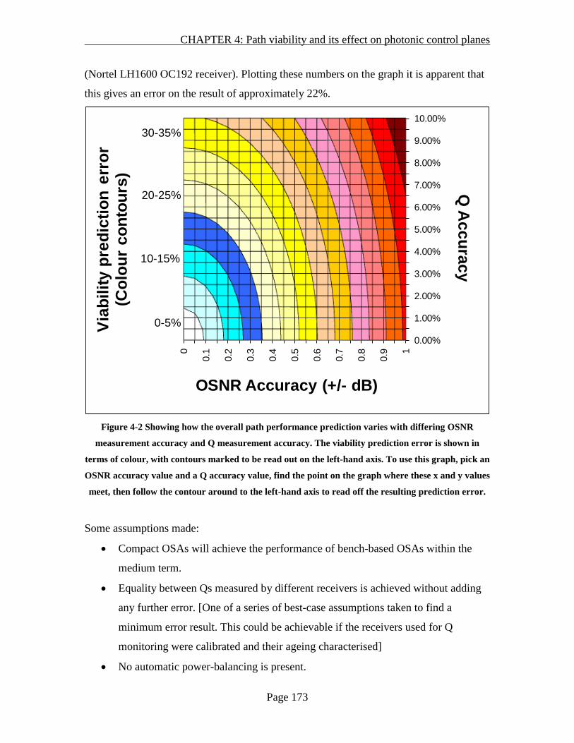
CHAPTER 4: Path viability and its effect on photonic control planes
Page 173
(Nortel LH1600 OC192 receiver). Plotting these numbers on the graph it is apparent that
this gives an error on the result of approximately 22%.
0.00%
1.00%
2.00%
3.00%
4.00%
5.00%
6.00%
7.00%
8.00%
9.00%
10.00%
0
0.1
0.2
0.3
0.4
0.5
0.6
0.7
0.8
0.9 1
Q A
ccuracy
OSNR Accuracy (+/- dB)
10-15%
0-5%
20-25%
30-35%
Viab
ility
pre
dict
ion
erro
r (C
olou
r co
ntou
rs)
Figure 4-2 Showing how the overall path performance prediction varies with differing OSNR
measurement accuracy and Q measurement accuracy. The viability prediction error is shown in
terms of colour, with contours marked to be read out on the left-hand axis. To use this graph, pick an
OSNR accuracy value and a Q accuracy value, find the point on the graph where these x and y values
meet, then follow the contour around to the left-hand axis to read off the resulting prediction error.
Some assumptions made:
• Compact OSAs will achieve the performance of bench-based OSAs within the
medium term.
• Equality between Qs measured by different receivers is achieved without adding
any further error. [One of a series of best-case assumptions taken to find a
minimum error result. This could be achievable if the receivers used for Q
monitoring were calibrated and their ageing characterised]
• No automatic power-balancing is present.

CHAPTER 4: Path viability and its effect on photonic control planes
Page 174
No non-linear effects impair the signal. [Hiew 06] shows that for 40GBaud this
assumption starts to break down for even smaller networks. However, as many 40Gbps
systems are using QPSK and/or polarization multiplexing to achieve a symbol rate of as
little as 10GBaud, the assumption is not broken by the 40Gbps systems of today.
Making an estimate of what might be a reasonable generational improvement in
equipment specification: 0.1 dB OSNR error and 3% Q error. This gives the dramatically
more useful ~12% path error. Significantly, this result is more accurate than the
specification-based planning-stage budgeting techniques of today.
The purpose of the second graph (Figure 4-3) is to show that 6 spans is not a number of
spans with any special significance – the error rises steadily with number of spans for
both the example hardware specifications.
0.00%
5.00%
10.00%
15.00%
20.00%
25.00%
30.00%
35.00%
3 4 5 6 7 8 9 10 11 12
% e
rror
of p
redi
ctio
n
Links/path
5%/0.25dB
3%/0.1dB
Figure 4-3 Performance prediction error rises steadily with the length of the path
4.3.9 The validity of measurements taken at a different fill level
Initial probing of the network is likely to occur at a lower fill level (number of
wavelength slots occupied) than will finally occur – and indeed, some transmitters etc.
may be installed as the network grows. In this and other circumstances, it is likely that the

CHAPTER 4: Path viability and its effect on photonic control planes
Page 175
measured wavelength will be running in a link with a different fill level than the
wavelength to be provisioned on that link – thus there is scope for the network
performance experienced to be somewhat different due to increased inter-channel
interference (e.g. FWM, XPM) as more wavelengths are added.
In the absence of per-wavelength dynamic VOA arrays, only two things change as the
number of wavelengths increases:
• Amplifier pump power increases to maintain a given level of gain.
• Non-linear effects due to total power in the fibre and also localised effects to
wavelengths adjacent to the newly added ones.
As has been previously stated, the latter point will be ignored as negligible at the power
levels considered.
Amplifier manufacturers claim that amplifier noise figures are near-constant for a given
gain, regardless of the pump power being used: a wavelength should suffer the same
added ASE if on its own or with e.g. 39 others.
4.3.10 Unmeasurable signal quality workaround
During practical experimentation on this architecture, a problem became apparent: Near
the transmitter, OSNR exceeded the ability of our OSAs to measure it accurately – the
signal had to pass through one or two EDFAs before the OSNR had reduced to being
measurable. To work around this, probe planning should note excessively high
measurements, discard them, and re-measure the same link by using a different probe
route whose transmitter is a few hops away. The consequence of this is that more probe
wavelengths will be required to get full coverage of the network. It also means that links
from terminal-only (i.e. no thru-capability) nodes cannot be measured.
CHAPTER 4: Path viability and its effect on photonic control planes
Page 176
4.4 Differences due to phase-modulated/coherent detection systems
As mentioned in Chapter 1, since the work described in this chapter was performed, the
coherent ‘revolution’ has occurred. The impact of the development of coherent detection
technology on this work can now be discussed. An example of the current commercial
state-of-the-art using coherent detection is provided in Appendix A.
Key differences and similarities between a conventional 10G on-off keyed (OOK) and a
Ciena 100G coherent (two-carrier dual-polarization quadrature phase-shift-keying, DP-
QPSK, see [OIF-FD-100G-DWDM] for details of the 100G standard based on this)
system are:
- Similarity: The symbol rate is approximately the same (12.5Gbaud/s) which gives
the same fundamental tolerance to effects such as PMD.
- Difference: The coherent receiver and DSPs can fully compensate for chromatic
dispersion and PMD in all new systems and most existing ones. This means that
coherent receivers can be used where it would be too expensive to retrofit the
network to support 10G OOK.
- Difference: As DP-QPSK is phase-modulated, the signal is affected by phase
noise from effects such as XPM more strongly than OOK.
- Difference: Q and OSNR calculations are different (but equivalent) because they
must take account of phase signal and noise rather than just amplitude.
Removing the need for DCMs (dispersion compensation modules) has the following
effects:
- The elimination of the capital cost of the DCMs and the engineering required to
calculate where to place them.
- The elimination of the significant power loss caused by the DCMs, and thus the
noise added by amplifiers to compensate for this loss. This makes more and
longer paths viable.
- Wavelength paths no longer need to achieve a narrow acceptable chromatic
dispersion range and so many more wavelength paths are viable – the A-B-C

CHAPTER 4: Path viability and its effect on photonic control planes
Page 177
chromatic dispersion example in the previous section no longer applies. It is this
advantage which is most significant for agile photonic networks because this key
reason for non-viability disappears in most practical cases.
- Neighbouring wavelengths ‘walk off’ each other more quickly (find their bit-
periods getting progressively more desynchronized as they are dispersed at every
hop rather than re-compensated), thus reducing XPM.
It is important to note that coherent systems are not incompatible with DCMs. Therefore
they may be used on existing fibre networks which mostly have DCMs present, still
offering significant advantages in bitrate, PMD tolerance etc.
Greenfield coherent deployments (i.e. where there are no existing OOK wavelength-
paths) have no requirement for DCMs. On non-dispersion-shifted fibre (e.g. the common
SMF-28e), in the absence of DCMs, the XPM penalty is reduced relative to an equivalent
fully-compensated modern many-channel 10G OOK system due to increased walk-off in
time between the signals’ symbols ([Thiele 00] describes the effects of XPM generally
and the interaction between XPM and walk-off length in depth), despite phase
modulation being more-directly affected by the phase noise of XPM than non-phase-
modulated OOK. This also applies to existing deployments where the DCMs and existing
non-coherent wavelengths have been removed. As mentioned, coherent receivers can
post-compensate for chromatic dispersion and polarization mode dispersion. Therefore,
the remaining dominant impairment may be noise. Therefore, an approximate impairment
calculation for coherent can be performed solely using OSNR as shown for OOK in
section 4.3.2. Quantifying the size of the error in this approximation, and whether it can
or should be approximated by some simple margin calculation, is discussed in the further
work section of Chapter 5.
Modern transmitter/receiver pairs based on digital-to-analogue and analogue-to-digital
converters are not fixed in hardware to any particular modulation format (e.g. QPSK, 8-
PSK, 16-QAM) so it may be possible to change in software or firmware. As such, a
trade-off between reach and bit-rate can be made. [Rival 11] demonstrates that by trading

CHAPTER 4: Path viability and its effect on photonic control planes
Page 178
off between bitrate and reach, because of reduced regeneration, port-counts may be
reduced. Rival et al. demonstrate up to a 21% reduction in the number of opto-electronic
ports required to serve their example European network by using flexible-rate
transponders. Such multi-format adaptive transmission is discussed further in [Friskney
02c], a US patent granted after examination, but otherwise out of scope of this thesis.
4.5 Chapter summary
A formal definition of optical viability within control planes was provided. Alternative
methods of pre-determining viability were reviewed. A new calculation of the error
involved in prediction based on live impairment measurement (a ‘measure-and-predict’
system) was provided.
This error calculation showed that given likely measurement accuracies (0.25dB OSNR
error, 5% Q error), a measure-and-predict system was less accurate (22%) than the
apparently more naive specify-and-predict approach, despite incurring the cost of
additional measurement hardware. Therefore measurement accuracies would need to
improve to make measure-and-predict a preferable choice. A combination that would
achieve this would be 0.1dB OSNR error and 3% Q error.
Until measurement equipment can be improved, the two options available for viability
calculation are then:
- Optical islands, only efficient where there are natural boundaries for other reasons
that can be made to align with unregenerated reach limits.
- Specify-and-predict systems.
An alternative viability prediction calculation would have a different error result. In
particular, if as has been speculated a purely noise-based viability calculation is
sufficiently precise for a coherent system, the above accuracy result would not apply.
‘Try it and see’ was shown to be unsuitable for a system that may require regeneration.

CHAPTER 4: Path viability and its effect on photonic control planes
Page 179
Finally, differences in impairment calculations between traditional on-off keyed (OOK)
modulation (the majority of the installed base of equipment) versus phase-modulation
with coherent reception (the direction of newer products, notably at 100Gbits/s per
wavelength) were described.
4.6 Statement of collaboration
The first (OOK) phase of the work described in this chapter was a project performed by
my team at Nortel’s Optical Communications Advanced Technology group and
documented in [Friskney 02a] and published in [Friskney 02]. The measure and predict
framework was proposed by Kevin Warbrick and Xiang Lu. The Q and OSNR equations
were written by me from references provided by and with validation from Richard Hearth
and Simon Poliakoff. The detailed error propagation equations were derived by me. The
first simplification was done by Simon Poliakoff. The generalisation of this to the full
range of input values, comparison with equipment behaviour and against network
accuracy was performed by me. The write-up was done exclusively by me, re-using some
material I contributed to [Friskney 02a] and [Friskney 02].
Work on viability approaches was done in collaboration primarily with Bram Peeters,
Duncan Forbes and Jim Shields (all then at Nortel) and co-patented as [Peeters 03]. This
write-up was provided by me, as a more comprehensive treatment than the summary
provided by Bram Peeters in [Peeters 04], and with criteria for comparison. Related work
was co-patented as [Shields 03].
The coherent section was written by me. I acknowledge very helpful conversations with
David Boertjes, Michael Morey and Alan Robinson and suggestions from Kim Roberts
(all while working for Ciena).
The principle of [Friskney 02c] was due to me, and then was developed in detail in
collaboration with the help of my listed co-inventors.

CHAPTER 4: Path viability and its effect on photonic control planes
Page 180
4.7 Chapter references
[Acreo 10] Acreo, “PRESS RELEASE: Acreo performed successful 100G DWDM field
trial using 16-QAM with advanced modulation and detection techniques”.
http://www.acreo.se/templates/Page____9477.aspx
[Agrawal 97] G. Agrawal, “Fiber-Optic Communication Systems”, Second Edition. John
Wiley & Sons, Inc., 1997.
[Agrawal 95] G. Agrawal, “Nonlinear Fiber Optics”, Second Edition. Academic Press,
1995.
[Ali 01] M. Ali, D. Elie-Dit-Cosaque, L. Tancesvki, “Enhancements to Multi-Protocol
Lambda Switching (MPlS) to Accommodate Transmission Impairments”. IEEE Global
Telecommunications Conference (Globecom) 2001 (25th-29th
[Duthel 08] T. Duthel, C. Fludger, J. Geyer, C. Schulien, “Impact of Polarisation
Dependent Loss on Coherent POLMUX-NRZ-DQPSK”. Optical Fiber Communication
November 2001), San
Antonio, Texas, USA, pp70-75.
[Azodolmolky 09] S. Azodolmolky et al., “A Dynamic Impairment-Aware Networking
Solution for Transparent Mesh Optical Networks”. IEEE Communications Magazine,
Vol. 47, Issue 5 (May 2009), pp 38-47.
[Belanger 06] Belanger, M.P, Cavallari, M. “Network cost impact of solutions for
mitigating optical impairments: comparison of methods, techniques, and practical
deployments constraints”. Journal of Lightwave Technology Vol. 24, Issue 1 (Jan 2006).
[Bernstein 10] G. Bernstein, Y. Lee, M. Kattan, “Information Model for Impaired Optical
Path Validation”. Internet Engineering Task Force (IETF) draft, draft-bernstein-wson-
impairment-info-03, October 2010.

CHAPTER 4: Path viability and its effect on photonic control planes
Page 181
and the National Fiber Optical Engineers Conference (OFC/NFOEC) 2008 (24th-28t
February 2008), San Diego, California, USA, p1-3.
[Friskney 02] R. Friskney, K. Warbrick, S. Poliakoff, R. Heath, "Link-based photonic
path performance prediction and control". 28th European Conference on Optical
Communications (ECOC) 2002 (September 2002), Copenhagen.
[Friskney 02a] R. Friskney, E. Pittuck, S. Poliakof, K. Warbrick, “Measurement-based
Dynamic Path Performance Prediction for Route Selection in Meshed Photonic
Networks: Approach and evaluation of the use of OSNR and Q”. Nortel internal report
code PU061/Photonic_Networks/00003/1.0/rjf, 30th April 2002.
[Friskney 02c] R. Friskney, A. Sparks, R. Spagnoletti, Robin Rickard, “Optical
Communications System”, US filing 10/180,595, filed June 2002. Granted 30th December
2008 as US Patent 7,471,903.
[G.680] International Telecommunications Union Telecommuication Standardization
Sector (ITU-T) Study Group 15, “Physical transfer functions of optical network
elements”. Recommendation G.680 (07/2007).
[GR-253-Core] Telcordia “Synchronous Optical Network (SONET) Transport Systems:
Common Generic Criteria”, GR-253-Core, Issue 4 (December 2005).
[Grosso 09] P. Grosso, D. Marchal, J. Maasen, E. Bernier, L. Xu, C. de Laat, “Dynamic
photonic lightpaths in the StarPlane network”. Future Generation Computer Systems,
Vol. 25, Issue 2 (February 2009), pp 132-136.
[Guild06] K. Guild, “Ultra-Fast Optical Routing including Impairment Constraints
(UFORIC)”. International Conference on Photonics in Switching 2006 (16th-18th October
2006), Heraklion, Greece, pp167-168.

CHAPTER 4: Path viability and its effect on photonic control planes
Page 182
[He 10] K. He, X. Li, “An Efficient Approach for Time-Domain Simulation of Pulse
Propagation in Optical Fiber”. Journal of Lightwave Technology, Vol. 28, Issue 20 (15th
October 2010), pp 2912-2918.
[Hiew 06] C.C. Hiew, F.M. Abbou, H.T. Chuah, S.P. Majumder, A.A.R. Hairul,
“Nonlinear BER performance of dense optical WDM manhattan street network with
deflection routing”. IEEE Photonics Technology Letters, Vol. 18, Issue 9 (May 1, 2006).
[Hui 09] R. Hui, M. O’Sullivan, “Fiber Optic Measurement Techniques”. Elsevier
Academic Press, 2009.
[Lee 04] L. Kwangil, M. A. Shayman, “Optical network design with optical constraints in
multi-hop WDM mesh networks”. 13th International Conference on
Computer Communications and Networks (ICCCN) 2004 (11th-13th October 2004),
Chicago, Illinois, USA, pp431-436.
[Lu 10] G-W. Ly, M. Skold, P. Johanisson, J. Zhao, M. Sjodin, H. Sunnerud, M.
Westlund, A. Ellis, P. Andrekson, “40-Gbaud 16-QAM transmitter using tandem IQ
modulators with binary driving electronic signals”. Optics Express Vol. 18, Issue 22 (25th
October 2010), pp 23062-23069.
[Millar 10] D. Millar, S. Makovejs, C. Behrens, S. Hellerbrand, R. Killey, P. Bayvel, S.
Savory, “Mitigation of Fiber Nonlinearity Using a Digital Coherent Receiver”. IEEE
Journal of Selected Topics in Quantum Electronics, Vol. 16, No. 5 (September/October
2010).
[Mishra 10] A.K. Mishra, A.D. Ellis, L.P. Barry, “Time-Resolved Q-factor Measurement
and Its Application in Performance Analysis of 42.6 Gbit/s Packets Generated by
SGDBR Lasers”. Journal of Lightwave Technology, Vol. 28, No. 8 (15th April 2010),
pp1144-1151

CHAPTER 4: Path viability and its effect on photonic control planes
Page 183
[OIF-FD-100G-DWDM] Optical Internetwork Forum (OIF) Implementation Agreement
OIF-FD-100G-DWDM-01.0 “100G Ultra Long Haul DWDM Framework Document”.
June 2009. http://www.oiforum.com/public/documents/OIF-FD-100G-DWDM-01.0.pdf
[Peeters 03] B. Peeters, R. Friskney, J. Shields, “Method of and system for routing in a
photonic network”. US filing 10/656,543, filed September 2003. Granted 13th January
2009 as US Patent 7,477,843.
[Peeters 04] B. Peeters, D. Forbes, R. Friskney, J. Shields, "Optimal routing in hybrid
networks by decoupling the route calculation from the assessment of optical route
viability", 9th European Conference on Networks & Optical Communications (NOC)
2004 (June 2004), Eindhoven, Netherlands.
[Qin 10] Y. Qin, Y. Pointurier, E. Escalona, S. Azodolmolky, M. Angelou, I. Tomkos, K.
Ramantas, K. Vlachos, R. Nejabati, D. Simeonidou, "Hardware accelerated impairment
aware control plane”. Optical Fiber Communication and the National Fiber Optical
Engineers Conference (OFC/NFOEC) 2010 (21st-25th March 2010), San Diego,
California, USA, p1-3.
[Ramamurthy 99] Ramamurthy et al., “Impact of Transmission Impairments on the
teletraffic performance of Wavelength-Routed Optical Networks”. Journal of Lightwave
Technology, IEEE, Vol. 17, No. 10 (1999).
[Reimer 07] M. Reimer, “Modeling and simulation of Polarization Mode Dispersion and
Polarization Dependent Loss”. University of Waterloo, Ontario, Canada. MSc thesis.
2007.
[RFC4655] A. Farrel, J.-P. Vasseur, J. Ash, “A Path Computation Element (PCE)-Based
Architecture”. Internet Engineering Task-Force (IETF) Request For Comments 4655.

CHAPTER 4: Path viability and its effect on photonic control planes
Page 184
[Rival 11] O. Rival, G. Villares, A. Morea, “Impact of Inter-Channel Nonlinearities on
the Planning of 25–100 Gb/s Elastic Optical Networks”. Journal of Lightwave
Technology, Vol. 29, No. 9 (1st May 2011), pp1326-1334.
[Saleh 00] A.A.M. Saleh, “Transparent optical networking in backbone networks”.
Optical Fiber Communication Conference (OFC) 2000 (7th-10th March 2000), Baltimore,
Maryland, USA, Vol. 3, ThD7-1 -ThD7-3.
[Savory 06] S. Savory, F. Payne, A. Hadjifotiou, “Estimating outages due to polarization
mode dispersion using extreme value statistics”. Journal of Lightwave Technology Vol.
24 Issue 11 (Nov 2006), pp 3907-3913.
[Segarra 06] J. Segarra, V. Sales, J. Prat, “Queue Management and Priority Scheduling
Disciplines for QoS Control in Wavelength Routed OBS (WROBS) Access Networks”.
International Conference on Transparent Optical Networks (ICTON) 2006 (June 2006),
Volume 3, pp207-214.
[Shatalin 06] S.V. Shatalin, A.J. Rogers, “Location of High PMD Sections of Installed
System Fiber”. Journal of Lightwave Technology, Vol. 24, Issue 11 (Nov. 2006), pp 207-
214.
[Shields 03] J. Shields, R. Friskney, “Optical Routing and Service Activation”. US filing
10/656,544 5th September 2003.
[Skoog 06] R.A. Skoog, T.C. Banwell, J.W. Gannett, S.F. Habiby, M. Pang, M.E. Rauch,
P. Toliver, “Automatic Identification of Impairments Using Support Vector Machine
Pattern Classification on Eye Diagrams”. IEEE Photonics Technology Letters,
Vol.18, Issue 22 (15th Nov 2006).
[SMF-28e] Corning SMF-28e datasheet, downloaded 2nd November 2008.

CHAPTER 4: Path viability and its effect on photonic control planes
Page 185
[Thiele 00] H. J. Thiele, “Investigation of high-speed optical transmission in the presence
of fibre nonlinearities”. PhD thesis, July 2000, University College London.
[Tintor 08] V. Tintor, P. Matavulj, J. Radunovic, “Analysis of blocking probability in
optical burst switched networks”. Photonic Network Communications Vol. 15 Issue 3
(June 2008).
[Tipsuwannakul 10] E. Tipsuwannakul, M. Chughtai, M. Forzati, J. Martensson, P
Andrekson, M. Karlsson, “Influence of self- and cross-phase modulation on 40 Gbaud
dual polarization DQPSK/D8PSK signals in 10 Gbit/s OOK WDM systems”. Optics
Express Vol. 18, Issue 23 (8th November 2010), pp 24178-24188.
[Um 08] T.W. Um, J.K. Choi, J. Guo, W. Ryu, B.S. Lee, “Soft-state bandwidth
reservation mechanism for slotted optical burst switching networks”. ETRI Journal
Vol. 30 Issue: 2 (April 2008).
[van den Borne 09] D. van den Borne, V. Sleiffer, M. Alfiad, S. Jansen, T. Wuth,
“POLMUX-QPSK modulation and coherent detection: the challenge of long-haul 100G
transmission”. 35th European Conference on Optical Communication (ECOC 20th-24th
September 2009).
[Wegmuller 04] M. Wegmuller, F. Scholder, N. Gisin, “Photon-counting OTDR for local
birefringence and fault analysis in the metro environment”. Journal of Lightwave
Technology. Vol. 22, Issue 2 (Feb. 2004).
[Winter 09] M. Winter, C.-A. Bunge, D. Setti, K. Petermann, “A Statistical Treatment of
Cross-Polarization Modulation in DWDM Systems”. Journal of Lightwave Technology,
Vol. 27, No. 17 (1st September 2009).
[Wson-impairments] Y. Lee, G. Bernstein, D. Li, G. Martinelli, “A Framework for the
Control of Wavelength Switched Optical Networks

CHAPTER 4: Path viability and its effect on photonic control planes
Page 186
(WSON) with Impairments”. Internet Engineering Task-Force (IETF) draft of the
Common Control and Measurement Working Group (CCAMP), draft-ietf-ccamp-wson-
impairments-04.
[Ye 07] D. Ye, W.D. Zhong, “Identifying various impairments of optical channels using
amplitude histogram”. Optical Engineering Vol. 46, Issue 12 (Dec 2007).
[Yen 07] Y. Hong-Hsu, S.S.W. Leeswlee, B. Mukherjee, “Impairment-aware Waveband
Switching in Optical Networks”. Optical Fiber Communication and the National Fiber
Optical Engineers Conference (OFC/NFOEC) 2007 (25th-29th March 2007), Anaheim,
California, USA, p1-3.
[Zapata 03] A. Zapata, P. Bayvel, “Impact of burst aggregation schemes on delay in
optical burst switched networks”. IEEE Lasers and Electro-Optics Society (LEOS) 2003
(27th-28th October 2003), Arizonia, USA, pp57-58.
[Zapata 04] A. Zapata, P. Bayvel, “Optimising scheduling delay in wavelength-routed
optical burst switched networks with re-attempt capability”. Optical Fiber
Communication Conference (OFC) 2004 (23rd-27th Feb 2004), Vol. 2, p3.
[Zhang 07] Z. Zhang, X. Bao, Q. Yu, L. Chen, “Time evolution of PMD due to tides and
sun radiation on submarine fibers”. Optical Fiber Technology, Vol. 13, Issue. 1 (January
2007), pp 62-66.

CHAPTER 5: Conclusions and further work
Page 187
Chapter 5 Conclusions and further work The work described in the thesis investigated the features of control plane functionality
for routing wavelength paths in telecommunications networks. The objective of this
routing functionality is to serve a set of changing sub-wavelength demands. Optimal
efficiency in terms of wavelength capacity required to serve a given set of demands is the
primary concern of this thesis. The work described in the thesis also takes account of
routing problems not found in higher Open Systems Interconnect (OSI) layers (e.g.
Ethernet, IP), notably physical transmission impairments. Agile wavelength-routed
optical networks (A-WRONs) were investigated as being the closest to currently-
deployed networks, and wavelength path sharing (WPS) as a variant on that that does not
require fast (per-packet, per-burst) switching such as optical burst switching (OBS) or
optical packet switching (OPS).
Firstly, the wavelength path sharing (WPS) scheme was discussed. WPS is a method of
reducing the need for photonic agility by allowing semi-static wavelengths to be a
unidirectional photonic shared-bus between multiple transmitters/receivers, allowing
statistical packet multiplexing. An alternative hardware configuration was proposed in
Chapter 2 (wavelength path sharing) which provided an additional benefit of photonic
networking (format transparency) and savings in receiver/transmitter hardware, the
quantitative benefit realised being according to the acceptable blocking probability
threshold selected by the operator and traffic levels.
The routing ILP originally proposed with the WPS scheme was found to not scale to
larger real-world networks. Therefore, a new heuristic was proposed.
This heuristic was shown to provide somewhat inferior performance (approx 50% more
wavelengths) relative to the ILP in terms of wavelength consumption efficiency as would
be expected, but still providing a significant gain (approx 20%) over the Baroni
theoretical lower bound of wavelength usage for A-WRONs with faster execution time
(approx 70%) with larger networks.
CHAPTER 5: Conclusions and further work
Page 188
Further simulations were executed looking at first-fit wavelength allocation in terms of
minimising continuous wavelength requirements, as this is a more practical parameter for
network dimensioning than an abstract count of wavelengths. Validating the simulations
using a new wavelength-allocation ILP showed that the first-fit algorithm noticeably
favoured the routes found by the heuristic over those found by the routing ILP – by
approximately 35%. This showed that comparing routing algorithms by combining them
with the first-fit algorithm will give misleading results relative to an optimal (e.g. ILP)
wavelength allocation, because the proportional ‘cost’ (sub-optimality in terms of
wavelengths consumed) of first-fit may be systematically biased towards one algorithm,
as it is here.
Using the optimal wavelength allocation results did not change the conclusion from the
earlier simulations. However, introducing a novel WPS routing algorithm based on AUR-
F offered a scalable algorithm at a low cost in wavelength utilisation (averaging 12%
more wavelengths across all topologies tested) relative to the ILP formulation given the
traffic and other assumptions stated in the chapter.
Secondly the question of how agile the WRON should be was addressed quantitatively in
Chapter 3. A formal definition of network agility was provided, and a simple mapping to
switch agility described. Modern switch technologies were compared in terms of agility
and a categorisation by function – configuration/restoration/protection/OBS/OPS, noting
that human provisioning does appear on this scale – was provided.
The quantitative network benefit that can be achieved by increased agility was assessed
by simulation. It was observed that the benefit achieved depended significantly upon the
network load – too low (negligible amounts of blocking) and there was nothing to
improve on; too high and the network achieved inoperable amounts of blocking. Within
the optimal window of load (with the network running at an average link-fill above 50%),
an improvement of 46% usable network capacity could be achieved against a maximum
acceptable blocking probability of 1% at the cost of a one thousand-fold increase in
network agility – the equivalent of moving into the next technology category faster. This

CHAPTER 5: Conclusions and further work
Page 189
is a significant and worthwhile efficiency improvement. It was observed that for a given
network size, the resulting signalling latency sets an upper bound on the value that can be
achieved by faster switching.
Finally, photonic viability - the question of whether a path that the control plane can
configure will work with sufficient bit error rate (BER) despite the physical transmission
impairments encountered – was reviewed in Chapter 4, both for conventional networks
and those based on the recently-commercialised coherent-receiver technology.
A formal definition of optical viability within control planes was provided. Alternative
methods of pre-determining viability were reviewed. A new calculation of the error
involved in prediction based on live impairment measurement (a ‘measure-and-predict’
system) was provided.
With this error calculation and given likely measurement accuracies, it was shown that a
measure-and-predict system was less accurate than the apparently more naive specify-
and-predict approach, despite incurring the cost of additional measurement hardware.
Therefore measurement accuracies would need to improve to make measure-and-predict
a preferable choice.
Until the measurement equipment (OSAs and Q monitors) can be improved, the two
options available for viability calculation are then:
- Optical islands, only efficient where there are natural boundaries for other reasons
that can be made to align with unregenerated reach limits.
- Specify-and-predict systems.
‘Try it and see’ was shown to be unsuitable for a system that may require regeneration.
Finally, differences in impairment calculations between conventional on-off keyed
(OOK) modulation (the majority of the installed base of equipment) versus phase-
CHAPTER 5: Conclusions and further work
Page 190
modulation with coherent reception (the direction of newer products, notably at
100Gbits/s per wavelength) were described.
In summary, improved routing techniques for both the WPS and A-WRON cases have
been provided, and recommendations were made for how to incorporate optical viability
(also known as impairment awareness) into these algorithms. These answer the original
research question of how a control plane routing algorithm can best serve sub-wavelength
demands with a wavelength-routed network.
The significance of the work is that it has:
- made WPS more practical for control planes by providing an efficient heuristic
algorithm for route calculation that is much faster than Myers’ ILP. The latter is
only really suitable for up-front planning where time is not an issue;
- brought new understanding to the value of agility by showing that under some
conditions (operators who never allow network load to get high), there may be no
value achieved – so they could buy a cheaper less-agile network. And to quantify
the value for suitable networks;
- determined the best viability calculation approach for a photonic control plane
to take (specify-and-predict - unless the network naturally splits into optical
islands), having reviewed the alternatives and exposed a problem of accuracy with
the proposed measure–and-predict approach.
Possible further work to extend that described in this thesis would be to:
- Calculate the viability error with a measure-and-predict system for a coherent
system using a noise-only approach and (for comparison) using a noise +
impairments approach. Theoretically the noise error calculation provided in
Chapter 4 should translate without modification to the coherent case. However,
the noise-only approach has not been publicly compared to
measurement/simulation at the time of writing and so some refinement of it may
CHAPTER 5: Conclusions and further work
Page 191
be required to achieve usable accuracy which may invalidate the assumption in
Chapter 4 of Gaussian noise for the coherent case and require an update of the
calculations. The noise + impairments approach would additionally require an
error calculation on the split-step Fourier calculation of the non-linear
impairments.
- Quantify the value of agility in a WPS system. The A-WRON-based calculations
of the value of agility should give an upper-bound on the value of agility in WPS
because WPS uses wavelength-paths for its communication. However, the use of
statistical multiplexing means that it is more tolerant to demand changes because
each unit of spare capacity within a wavelength-path is available to two different
demands. Simulations similar to that provided in Chapter 3 could be used to
quantify how much difference this made.
- Provide routing algorithms that simultaneously optimise cost and achieve
viability. The scaling problems of multi-objective optimisation are well known
([Reinhardt 11] is a very recent paper providing a survey). In the past, this has
been avoided by assuming that cost and viability are correlated and optimising
just for viability. It is indeed the trend that cost rises with distance (due to
increased fibre and equipment traversed), and the probability of viability falls
(due to increased accumulated impairments). Therefore many solutions have
simply optimised on viability. However, the correlation is not total. As per the
Deutsche Telekom PMD study [Breuer 03] discussed at length in Chapter 1, in
older networks a lot of highly-impaired fibre exists which a solution optimising
on viability would avoid. However, these fibres are likely to be lower-cost
because the service provider wishes them to be used for any traffic that can to free
up less-impaired links for wavelength-paths. For this reason, impairment should
be treated as a binary threshold (as discussed in the next paragraph) rather than an
optimisation parameter.

CHAPTER 5: Conclusions and further work
Page 192
- Provide routing algorithms that achieve a given maximum cost goal. For viability
as mentioned in the previous paragraph and cost factors such as latency – a
requirement that I have seen become more commercially significant in my
industrial experience – there is a threshold value above which a service is simply
not useful (e.g. it exceeds the latency guarantee of a particular contract type, or
the maximum tolerable latency of a particular application) and therefore highly
costly routes become the only option. Techniques such as exception routing
(described in many papers e.g. the Nortel-sponsored [Ahmed 09] and its
references) can address this binary acceptability problem, at a cost in scalability –
[Ahmed 09] gets the cost down to a constant factor which is the number of
exceptions that need to be made (routes tried that are known not to be valid).
These techniques are problematic in practice because the algorithms tend to try
every variant on the failed path (all of which are also invalid), as these are of
similar cost, before trying a different but slightly more costly approach, so the
number of exceptions can become large. Therefore, there is opportunity for a
viability-specific algorithm that understands viability to have a significant scaling
advantage.
- Calculate the efficiency loss in wavelength usage terms of the viability calculation
error. A worst-case model could be taken of a reduction in reach (and thus
increased use of regenerators) equivalent to the size of the error bar in viability
calculation.
- Develop a signalling protocol that would allow a distributed specify-and-predict
algorithm to function. Extending OSPF-TE or ISIS-TE in this way would be
straightforward. However, there could be some implications. In terms of
propagation latency of impairment information, theoretically the loss and
amplifier noise factors required for an OSNR-based solution are near-constant
(decaying over the course of years rather than hours). If the nonlinear
impairments were calculated using specify-and-predict based on equipment
manufacturer data for a worst-case then these also would not vary, whereas with

CHAPTER 5: Conclusions and further work
Page 193
measure-and-predict they would vary with each added wavelength. If a coherent
approach using an elaborate nonlinear impairment calculation approach with
many parameters per link were used, then scaling might become a concern for
larger networks.
- Devise multi-layer routing algorithms that would simultaneously optimise the
photonic and client layers, still taking account of optical viability. This should
produce better results than separate optimisation. For example, an alternative to
setting up a lightpath A-B for a small amount of new traffic may be to indirect the
traffic via existing lightpaths with spare capacity A-C and C-B. This has the
benefit of decreasing the number of wavelengths required. It has the cost of
requiring additional electronic switching capacity at C. However, this indirection
should not always be done: it also hastens both A-C and C-B requiring an
additional wavelength. Where C is not along an optimal path for A-B, this
indirection action may at a later time therefore cause more wavelength-links to be
consumed than if it had not been done.
5.1 References
[Ahmed 09] M. Ahmed, A. Lubiw, “Shortest paths avoiding forbidden subpaths”.
26th
International Symposium on Theoretical Aspects of Computer Science (STACS),
Freiburg 2009, pp 63-74.
[Breuer 03] D. Breuer, H-J. Tessmann, A. Gladisch, H. Foisel, G. Neumann, H. Reiner,
H. Cremer, “Measurements of PMD in the installed fiber plant of Deutsche Telekom”.
LEOS Summer Topical Meetings 2003, Holey Fibers and Photonic Crystals/Polarization
Mode Dispersion/Photonics Time/Frequency Measurement and Control, 14th-16th
July
2003, MB2.1/5.
[Reinhardt 11] L.B. Reinhardt, D. Pisinger, “Multi-objective and multi-constrained non-
additive shortest path problems”. Computers and Operational Research Vol. 38, Issue 3
(March 2011), pp605-616.

APPENDIX A: Case study
Page 194
Appendix A A case study of the current state of the commercial art: The Ciena Photonic Layer with 40Gbps and 100Gbps/channel DWDM transmission
This appendix is frequently referenced in the main part of the thesis as an example of
what is being deployed in volume commercially at the time of writing. The other chapters
reference particular aspects and characteristics of the Ciena solution, this appendix gives
context to those attributes. As will be seen, while most of the network functions used in
the remainder of the thesis (amplifiers, DWDM multiplexers/demultiplexers, VOAs,
power monitors etc.) are part of this real product, the way they are designed to be used
here (e.g. with turn-up times reported in 2009 as “around 10 minutes” [Grosso 09],
although current performance not public) is a long way from the millisecond or
nanosecond timescales discussed in some papers at present (reviewed in Chapter 3). At
the end of the appendix, the implications on control plane agility of the Ciena system
design choices are described.
The Ciena coherent transmission system is a good example because it has been very
commercially successful – [Ciena 11c] states that, as of 19th
A.1 Disclaimers
May 2011, Ciena “has
shipped in excess of 7,000 coherent 40G/100G line interfaces to more than 80 customers
across the globe with more than 5.5 million coherent kilometres deployed”.
Disclaimers: No part of this thesis should be taken to form any kind of statement, claim,
commitment or other form of communication by or on behalf of Ciena. This section is a
summary of public information, and may not take account of commercially confidential
information known to the author.
Copyright in the diagrams in this chapter is owned by Ciena. They are reproduced here
with permission.
APPENDIX A: Case study
Page 195
A.2 The Ciena Common Photonic Layer (CPL) and 6500 Photonic Layer
This section describes an example of the current state of the commercial art in the field.
Ciena CPL was formerly known as Nortel CPL.
Ciena 6500 Photonic Layer was formerly known as Nortel OME6500 Photonic Layer.
The Ciena 6500 Photonic Layer is, for the purposes of this thesis, a physically-
repackaged version of the CPL – within a chassis capable of many higher-layer functions
- and therefore they will not be separately described.
This section is a summary of [Nortel 07] and [Ciena 11a]. The Common Photonic Layer
is the overall brand within Ciena for a system of optical amplifiers, DWDM
multiplexers/demultiplexers (mux/demuxes) and related components. A diagram of the
system is provided below in Figure A-1. It was introduced to simplify usage of the
photonic layer through automation and network intelligence; to service a range of reaches
(metro, regional and long-haul deployments); and to scale both up and down effectively –
i.e. be suited to small initial deployments that could incrementally add wavelengths later
without disrupting those already in service (e.g. by requiring them to be temporarily
unplugged for additional components to be inserted into the line).
The Domain Optical Control (DOC) system is a software-based automatic wavelength
turn-up and power optimisation systems. This is a significant part of CPL because some
previous systems have required manual turn-up such as people with screwdrivers
adjusting or adding/removing optical attenuators. Automatic turn-up not only decreases
the time and cost taken to introduce new wavelengths, but reduces the risk of errors, i.e.
decreases the chance that existing wavelengths will be disrupted. A reduced risk of
disruption of existing traffic makes it more acceptable to introduce wavelengths during
normal operation rather than in special maintenance windows that have to be agreed with
all existing customers some time (e.g. weeks) in advance.
APPENDIX A: Case study
Page 196
Part of the objective of CPL and DOC was to allow more sophisticated photonic
topologies to be supported. In particular, to add support for photonic branching. This is
defined as the point where at an OADM site, dropped wavelengths may then go into
another line system (through amplifiers not on the first line system). This contrasts to
local termination, where the optical receivers are physically co-located with the OADM
device, so no further amplification is required. The reason that branching support is
challenging is because the automatic power optimisation must simultaneously optimise
the interlinked operation of multiple line systems, rather than being constrained to a
simple linear segment.
A further benefit offered by DOC is that a planning tool is available that contains the
DOC algorithm, plus continuous monitoring and re-optimisation allows initial
performance to be increased by using initial link margins appropriate for the exact
configuration used, rather than a conservative general-purpose figure. Note that this
direct measurement of end-to-end BER is not what is in the link-by-link measurement
model described in Chapter 4, where path prediction based on measured link-by-link
characteristics was shown to be less accurate than specification-based predictions.
The CPL provides support for up to 88 wavelengths on the C-band with 50GHz
wavelength spacing, or 44 wavelengths with 100GHz spacing, both using the standard
ITU grid [G.694.1] of channel frequencies. This is achieved in two stages, a 4- or 8-
channel (100GHz or 50GHz respectively) mux/demux (CMD) module, followed by a 9-
way group mux/demux (GMD). The GMD also hosts the distributed power control plane
(GMD). As discussed below, each of the channels may be up to 100Gbps, giving a total
system capacity of 7.2Tbps/fibre. [Nortel 08] and [Ciena 10a] describes achieving 88
100Gbps wavelengths by using a passive splitter with amplifier to two 44-way splitters,
giving a system capacity of 8.8Tbps/fibre. The previous Nortel long-haul transmission
system (LH1600G) supported 80 C-band wavelengths and optionally allowed a parallel
set of optical amplifiers/splitters/combiners to be used to achieve 80 wavelengths in the
L-band, allowing 160 wavelengths in total. CPL makes no attempt to support any part of
the fibre spectrum other than C-band at the time of writing.

APPENDIX A: Case study
Page 197
Figure A-1 The architecture of the Common Photonic Layer (CPL), showing that it can exclude
transmitters/receivers from its control domain and so can support any terminal device supporting a
support ITU grid wavelength – illustrated devices include metro photonics, long-haul photonics,
SDH/SONET multiplexers (including of non-TDM traffic) and large-scale enterprise Ethernet
switching. eROADM/WSS are discussed in the next section. Taken from [Nortel 07]
Extracted (dropped) wavelengths Inserted (added) wavelengthsλ1, λ2, λ3, λ4, λ5, … λ20, λ21, λ22, λ23, λ24,
…
WB blocks the desired wavelengths from passing through
and directs them to the filter for extraction (drop)
New wavelengths can be inserted (added) after the WB
Wavelength blocker (WB)
Figure A-2 Forming a ROADM for local termination/origination of wavelengths using a wavelength
blocker. Reproduced from [Nortel 06a]

APPENDIX A: Case study
Page 198
The CPL amplifier is locally gain-controlled but participates in the DOC and thus may
have its gain adjusted by this control plane. The amplifier is also transient-suppressed.
Both of these are to reduce the impact on existing wavelengths of addition/removal of
new/defunct wavelengths, as a planned operation or due to an upstream fault.
The reasons for the ‘common’ in the name is that CPL is intended to carry wavelengths
of all sources that can comply with the ITU grid as neighbours on the same fibre
(designed for 1.25-40Gbps wavelengths, 100Gbps compatible as discussed below) – from
short-reach traffic used by low-cost metro equipment, to extremely optically-performance
sensitive ultra-long-reach wavelengths. In particular, a design goal is to carry non-Ciena-
originated wavelengths - ‘alien’ wavelengths, as shown in Figure A-1. This new
capability is significant because alien wavelengths cannot be expected to participate in
the DOC control plane, or carry Ciena-proprietary health-monitoring data. Therefore, all
DOC signalling is done out-of-band, all channels are controlled by electronically-
controlled VOAs, and the DOC resides in the line system components rather than the
transmitter/receiver cards.
A.2.1 Wavelength Selective Switches (WSSs) for Reconfigurable Optical Add/Drop Multiplexers (ROADMs)
This section provides a summary of [Nortel 06a] and [Ciena 10a]. For its latest ROADM
product, Ciena has chosen to use micro electro-mechanical systems (MEMS)-based
wavelength selective switches (WSSs), which it brands as Enhanced Reconfigurable
Optical Add/Drop Multiplexers (eROADMs). WSSs allow the dropping of an arbitrary
choice of wavelengths into one of – with this product – five different output ports. Each
output port is truly ‘colourless’ and so can have any selection of wavelengths directed to
it by remote configuration, avoiding the bandwidth stranding of systems without this
capability such as PLC-based ROADMs. This makes branching sites simpler than with
the older technology of wavelength blockers (WB), which were two port devices,
selectively allowing/disallowing a wavelength through.

APPENDIX A: Case study
Page 199
Figure A-2 shows an equipment configuration where a WB is used for local add/drop. It
shows that selected wavelengths can be dropped when they reach the WB. A passive
coupler before the WB allows reception of those wavelengths, once selected via DWDM
demultiplexers. Selected wavelengths (either previously blocked or never inserted onto
the line) can be inserted, via passive coupler, after the blocker.
As will be clear, to form an n-way non-blocking cross-connection, n.n-1 WBs would be
required (one for each input to each output that does not loop back into the input fibre-
pair), with losses caused by n-way couplers becoming quickly unacceptable. WSSes are
preferable because only n would be required to provide a full cross-connection. The
solution publicly advertised by Ciena offers five-way branching with WSSes and use of
50GHz spacing, but only two-way and 100GHz spacing with WB or planar lightwave
circuits (PLC) approaches.
A.2.2 Colourless and direction-independent filters
Figure A-2 above includes traditional fixed multiplexer/demultiplexers. That is to say,
any particular port a transmitter/receiver plugs into will be for a designated wavelength.
Thus, if the transmitter is tunable, this facility cannot be utilised for route agility –
tunable transmitters provide value only in that one spare does not need to be kept for each
wavelength, as was the case with fixed transmitters.
This presents an obstacle to network agility when provisioning a new path – unless 88
spares (one/wavelength) are deployed, how can the control plane be sure it will find a
terminal or regenerator on the correct wavelength? If a spare terminal/regenerator is
installed on every wavelength, how can the network cost minimisation goals be met?
The solution to this is not to use fixed filters. Some vendors propose using tunable filters.
At present, our competitive information is that these result in an expensive solution.
Another solution would be to attach a transmitter/receiver directly to a ROADM port.
This would allow full flexibility as to which wavelength could be added/dropped, but
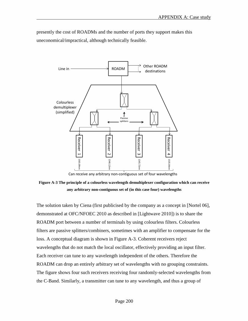
APPENDIX A: Case study
Page 200
presently the cost of ROADMs and the number of ports they support makes this
uneconomical/impractical, although technically feasible.
Receiver 1
Receiver 2
Receiver 3
Receiver 4
Colourlessdemultiplexer
(simplified)Passive splitters
ROADMOther ROADM destinationsLine in
1565.09nm
1546.12nm
1545.72nm
1535.04nm
Can receive any arbitrary non-contiguous set of four wavelengths Figure A-3 The principle of a colourless wavelength demultiplexer configuration which can receive
any arbitrary non-contiguous set of (in this case four) wavelengths
The solution taken by Ciena (first publicised by the company as a concept in [Nortel 06],
demonstrated at OFC/NFOEC 2010 as described in [Lightwave 2010]) is to share the
ROADM port between a number of terminals by using colourless filters. Colourless
filters are passive splitters/combiners, sometimes with an amplifier to compensate for the
loss. A conceptual diagram is shown in Figure A-3. Coherent receivers reject
wavelengths that do not match the local oscillator, effectively providing an input filter.
Each receiver can tune to any wavelength independent of the others. Therefore the
ROADM can drop an entirely arbitrary set of wavelengths with no grouping constraints.
The figure shows four such receivers receiving four randomly-selected wavelengths from
the C-Band. Similarly, a transmitter can tune to any wavelength, and thus a group of

APPENDIX A: Case study
Page 201
transmitters can inject an arbitrary set of wavelengths into the ROADM. This is the exact
converse of the figure.
b. Direction-independent terminal configuration
a. Direction-dependent terminal configuration
ROADM
Transmitter 1
Transmitter 4
Transmitter 3
Transmitter 2
Tran
smitt
er 5
Tran
smitt
er 8
Tran
smitt
er 7
Tran
smitt
er 6
ROADMLine out 1 Line out 2
ROADM
Transmitter 1
Transmitter 4
Transmitter 3
Transmitter 2
Transmitter 5
Transmitter 8
Transmitter 7
Transmitter 6
ROADMLine out 1 Line out 2
ROADM
Figure A-4 The principles of direction-dependent versus direction-independent terminal
configurations.
Directionally-independent operation is simply the concept that a particular transceiver is
not bound to a specific ‘direction’ (a particular fibre at a ROADM site). This concept is
illustrated in Figure A-4, which shows a subset of the hardware at a 2-direction (“Line
out 1” and “Line out 2”) ROADM site. The subset is just to show the path from the local
transmitters to their line systems. The diagram for receivers is just the converse, omitted
for simplicity. Other inputs from the ROADMs are also omitted for simplicity. Diagram a
shows an older-fashioned direction-dependent terminal configuration where e.g.
transmitter 1 is unconditionally associated with line out 2. Diagram b shows a direction-
independent (sometimes called ‘directionless’ in marketing material) node configuration
where each transmitter can output to any direction according to switch settings. Diagram
b requires a larger switching capability (an extra WSS as illustrated here, or one bigger
WSS, or some such), which has cost relative to diagram a. However, it will be more
efficient and flexible in how the transmitters may be used. Like colourless, direction-
APPENDIX A: Case study
Page 202
independent improves the value of speculative installation of transceivers/regenerators at
a site, because any one transceiver can be used for more directions.
To be clear, direction-independence uses no novel hardware or concepts of any fashion -
the innovation is to enable the power-balancing control plane to support this
configuration, which previously it did not.
A.3 The Ciena 40G transmission system
The Ciena 100G transmission system is based on the 40G system, so that is described
first. Both are currently implemented as transmitter/receiver cards for the 6500 chassis,
that also supports many other card types for functions such as TDM switching, packet
switching, adaptation of many traffic types (e.g. Ethernet, SAN, PDH, SDH, SONET), or
simple regeneration. The associated line system components (e.g. amplifiers,
mux/demuxes) form part of the previously-described Common Photonic Layer system or
may also reside in 6500 chassis.
The Ciena 40Gbps transmission product is able to upgrade existing 10G infrastructure
just by replacing transponders and achieve equivalent continental-scale (2000km+
[Nortel 08]) reach equivalent to Ciena’s more traditional (i.e. simple non-return-to-zero
(NRZ)-modulated) 10Gbps transmission systems1
1 Ciena now has an upgraded 10Gbps transmitter with electronic dispersion pre-compensation, branded as
electronic dynamic-compensating optics (eDCO) [Nortel 06]. The ‘traditional’ transmitter is given as a
reference point of the state of the art across the industry before digital signal-shaping/post-compensation
started to be used.
. By comparison, its competitors using
other technologies, such as non-polarization DQPSK, achieve distinctly limited reach and
require more constrained and idealised conditions – only certain fibre types, and more
tightly constrained dispersion maps – such that upgrading 10G systems can only be done
in rare circumstances, or by re-engineering the intermediate equipment. Therefore, while
Ciena’s approach results in more complex (and therefore potentially more expensive)
transponders, less of them are needed, the system cost for upgrading to 40G can often be
much lower, the upgrade can be done selectively per-wavelength rather than as one big
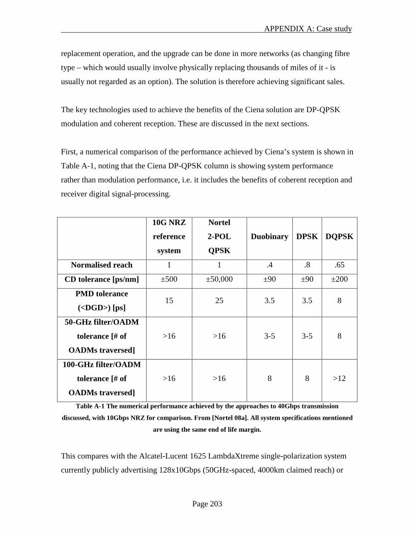
APPENDIX A: Case study
Page 203
replacement operation, and the upgrade can be done in more networks (as changing fibre
type – which would usually involve physically replacing thousands of miles of it - is
usually not regarded as an option). The solution is therefore achieving significant sales.
The key technologies used to achieve the benefits of the Ciena solution are DP-QPSK
modulation and coherent reception. These are discussed in the next sections.
First, a numerical comparison of the performance achieved by Ciena’s system is shown in
Table A-1, noting that the Ciena DP-QPSK column is showing system performance
rather than modulation performance, i.e. it includes the benefits of coherent reception and
receiver digital signal-processing.
10G NRZ
reference
system
Nortel
2-POL
QPSK
Duobinary DPSK DQPSK
Normalised reach 1 1 .4 .8 .65
CD tolerance [ps/nm] ±500 ±50,000 ±90 ±90 ±200
PMD tolerance
(<DGD>) [ps] 15 25 3.5 3.5 8
50-GHz filter/OADM
tolerance [# of
OADMs traversed]
>16 >16 3-5 3-5 8
100-GHz filter/OADM
tolerance [# of
OADMs traversed]
>16 >16 8 8 >12
Table A-1 The numerical performance achieved by the approaches to 40Gbps transmission
discussed, with 10Gbps NRZ for comparison. From [Nortel 08a]. All system specifications mentioned
are using the same end of life margin.
This compares with the Alcatel-Lucent 1625 LambdaXtreme single-polarization system
currently publicly advertising 128x10Gbps (50GHz-spaced, 4000km claimed reach) or
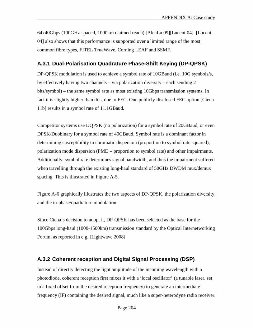
APPENDIX A: Case study
Page 204
64x40Gbps (100GHz-spaced, 1000km claimed reach) [AlcaLu 09][Lucent 04]. [Lucent
04] also shows that this performance is supported over a limited range of the most
common fibre types, FITEL TrueWave, Corning LEAF and SSMF.
A.3.1 Dual-Polarisation Quadrature Phase-Shift Keying (DP-QPSK)
DP-QPSK modulation is used to achieve a symbol rate of 10GBaud (i.e. 10G symbols/s,
by effectively having two channels – via polarization diversity – each sending 2
bits/symbol) – the same symbol rate as most existing 10Gbps transmission systems. In
fact it is slightly higher than this, due to FEC. One publicly-disclosed FEC option [Ciena
11b] results in a symbol rate of 11.1GBaud.
Competitor systems use DQPSK (no polarization) for a symbol rate of 20GBaud, or even
DPSK/Duobinary for a symbol rate of 40GBaud. Symbol rate is a dominant factor in
determining susceptibility to chromatic dispersion (proportion to symbol rate squared),
polarization mode dispersion (PMD – proportion to symbol rate) and other impairments.
Additionally, symbol rate determines signal bandwidth, and thus the impairment suffered
when travelling through the existing long-haul standard of 50GHz DWDM mux/demux
spacing. This is illustrated in Figure A-5.
Figure A-6 graphically illustrates the two aspects of DP-QPSK, the polarization diversity,
and the in-phase/quadrature modulation.
Since Ciena’s decision to adopt it, DP-QPSK has been selected as the base for the
100Gbps long-haul (1000-1500km) transmission standard by the Optical Internetworking
Forum, as reported in e.g. [Lightwave 2008].
A.3.2 Coherent reception and Digital Signal Processing (DSP)
Instead of directly detecting the light amplitude of the incoming wavelength with a
photodiode, coherent reception first mixes it with a ‘local oscillator’ (a tunable laser, set
to a fixed offset from the desired reception frequency) to generate an intermediate
frequency (IF) containing the desired signal, much like a super-heterodyne radio receiver.
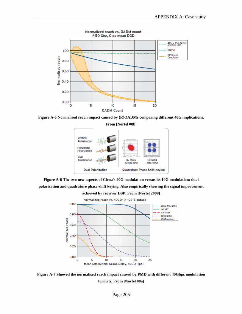
APPENDIX A: Case study
Page 205
Figure A-5 Normalised reach impact caused by (R)OADMs comparing different 40G implications.
From [Nortel 08b]
Figure A-6 The two new aspects of Ciena's 40G modulation versus its 10G modulation: dual
polarization and quadrature phase-shift keying. Also empirically showing the signal improvement
achieved by receiver DSP. From [Nortel 2009]
Figure A-7 Showed the normalised reach impact caused by PMD with different 40Gbps modulation
formats. From [Nortel 08a]

APPENDIX A: Case study
Page 206
This provides phase information as well as amplitude. Polarization diverse receivers
allow polarization information to be extracted. Given this much richer information
(amplitude, phase and polarization) than traditional systems (amplitude only), and digital
signal processing (DSP) including polarization tracking, the DP-QPSK can then be
demodulated. However, the DSP also has the information to undo chromatic and
polarization mode dispersion to the extent shown in Table A-1. In fact, the 40Gbps
system achieves better PMD tolerance (25ps) than the conventional NRZ 10Gbps system
(15ps), the network system impact of this is shown in Figure A-7. This means that some
fibres deemed unsuitable for 10Gbps transmission due to excess PMD can now be used
for 40Gbps.
Coherent technology has therefore provided a revolution in:
- Increased spectral efficiency to allow higher bitrates without increasing baud rate
and thus impairment sensitivity.
- Working with DSP to cancel out some impairments altogether, and ameliorate
others, to increase reach and make photonic systems easier to plan.
A.3.3 The Ciena 100G transmission system
Following on from the 40Gbps transmission system described above, Ciena has made
available its “40G/100G adaptive optical engine”. With the now-Ciena system, Nortel
was able to announce the first commercially-supplied 100G wavelength, and
(simultaneously) first commercial traffic to travel over 100G [Nortel 09] – the 893km
Paris-Frankfurt link for Verizon, added alongside in-service 10G wavelengths in the same
fibre. Further sales and field trials have followed, such as TelstraClear [Ciena 10] and
Surfnet [Ciena 11c].
As described in [Nortel 08], the Ciena 100G system uses similar modulation to the 40G
system, DP-QPSK, up-rated to 50G, then runs two such wavelengths 20GHz apart to
form a combined bit-rate of 100Gbps2
2 As with 10 and 40Gbps, this is not exactly 100Gbps due to FEC and other overheads. In particular, a key
published rate is ITU OTU-4, an OTN wrapper for 100GE, at 112Gbps before FEC.
(although the two wavelengths are produced,
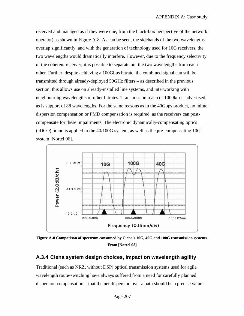
APPENDIX A: Case study
Page 207
received and managed as if they were one, from the black-box perspective of the network
operator) as shown in Figure A-8. As can be seen, the sidebands of the two wavelengths
overlap significantly, and with the generation of technology used for 10G receivers, the
two wavelengths would dramatically interfere. However, due to the frequency selectivity
of the coherent receiver, it is possible to separate out the two wavelengths from each
other. Further, despite achieving a 100Gbps bitrate, the combined signal can still be
transmitted through already-deployed 50GHz filters – as described in the previous
section, this allows use on already-installed line systems, and interworking with
neighbouring wavelengths of other bitrates. Transmission reach of 1000km is advertised,
as is support of 88 wavelengths. For the same reasons as in the 40Gbps product, no inline
dispersion compensation or PMD compensation is required, as the receivers can post-
compensate for these impairments. The electronic dynamically-compensating optics
(eDCO) brand is applied to the 40/100G system, as well as the pre-compensating 10G
system [Nortel 06].
Figure A-8 Comparison of spectrum consumed by Ciena's 10G, 40G and 100G transmission systems.
From [Nortel 08]
A.3.4 Ciena system design choices, impact on wavelength agility
Traditional (such as NRZ, without DSP) optical transmission systems used for agile
wavelength route-switching have always suffered from a need for carefully planned
dispersion compensation – that the net dispersion over a path should be a precise value

APPENDIX A: Case study
Page 208
(whatever amount of dispersion is naturally compensated for by the configured laser
chirp). If the net dispersion does not exactly match this target, the link budget will be
impaired and thus some paths will cease to work. Thus, net dispersion needs to be tracked
in such systems’ viability calculators or planning restrictions introduced with their own
negative consequences, such as exactly compensating each fibre span (requires very fine
granularity of DSCMs, or dispersion compensation fibre to be cut to length and spliced
on site, increases the non-linear interference between co-propagating wavelengths by
bringing them back into temporal correlation) or limiting the size of the network such that
the net dispersion is bounded.
However, if lumped dispersion compensation is not required, as in the Ciena system, this
problem simply does not exist. This applies both to new-build networks with no DSCMs
at all, and existing networks with DSCMs designed for statically-routed 10G wavelengths
– which can now be upgraded to flexibly-routed 40G paths. This is because, as well as
compensating for large amounts of dispersion, electronic dispersion compensation is also
useful for compensating for residual dispersion that varies with the route chosen, as can
occur in partially-compensated systems.
Eliminating bulk fibre dispersion slope compensation modules (DSCMs) has the
additional benefit of reducing latency (less distance for the light to travel) and OSNR
degradation caused by the additional amplifier required to compensate for the DSCM’s
loss.
The Ciena transmitters and receivers are tunable to the full-C-band of wavelengths. Other
transmission systems are not (such as the predecessor of CPL, the Nortel LH1600
system), which places restrictions upon routing and wavelength assignment.
In 2009 [Grosso 09] reported a complete wavelength turn-up time of “around 10
minutes” using a Nortel CPL system – CPL being the previous branding and physical
packaging for the Ciena 6500 photonic capability. 10 minutes would be fast enough for
APPENDIX A: Case study
Page 209
time-of-day based rerouting, but does not provide sufficient switching speed for
OBS/OPS. The current switching speed of the 6500 is not public information.
A.4 Chapter references
[AlcaLu 09] Alcatel-Lucent 1625 LambaXtreme Transport Technical Details.
http://www.alcatel-
lucent.com/wps/portal/products/detail?LMSG_CABINET=Solution_Product_Catalog&L
MSG_CONTENT_FILE=Products/Product_Detail_000044.xml&LMSG_SUBCATEGO
RY=Core+DWDM+Systems&LMSG_PARENT=Product_Families/Product_Family_000
026.xml&LMSG_CATEGORY=Optics#tabAnchor4. As captured March 2009.
[Ciena 10] Ciena, “TelstraClear Core Network Supports 100G for Ultra Fast Data
Speeds”. Press release. 6th July 2010.
[Ciena 11a] Ciena, “ActivSpan Common Photonic Layer”, Data Sheet. As captured
January 2011.
http://media.ciena.com/documents/ActivSpan_Common_Photonic_Layer_DS.pdf
[Ciena 11b] Ciena, “ActivFlex 6500 Packet-Optical Platform”, Data Sheet. As captured
January 2011.
http://media.ciena.com/documents/ActivFlex_6500_Packet_Optical_Platform_DS.pdf
[Ciena 11c] Ciena, “SURFnet Selects Ciena for Coherent 100G International Network”.
Press release. 19th
[Comcast 08] “Comcast, Nortel Put 100G to the test”.
May 2011. http://www.ciena.com/corporate/news-events/press-
releases/SURFnet-Selects-Ciena-for-Coherent-100G-International-Network.html.
http://www.lightreading.com/document.asp?doc_id=148259&site=cdn 12th March 2008.
Also Nortel press release http://www2.nortel.com/go/news_detail.jsp?cat_id=-
8055&oid=100237988&locale=en-US, 13th March 2008.
APPENDIX A: Case study
Page 210
[G.694.1] ITU-T, “Spectral Grids for WDM applications: DWDM frequency grid”.
Standard G.694.1, issued June 2002.
[Grosso 09] P. Grosso, D. Marchal, J. Maasen, E. Bernier, L. Xu, C. de Laat, “Dynamic
photonic lightpaths in the StarPlane network”. Future Generation Computer Systems,
Vol. 25, Issue 2, February 2009, pp132-136.
[Infonetics 08] Michael Howard (Principal Analyst), “Cost Considerations in 40G
Networks”, Infonetics Research, March 2008.
[Lightwave 2008] Meghan Fuller Hanna, “Is DP-QPSK the endgame for 100Gbits/sec”.
http://lw.pennnet.com/display_article/345073/13/ARTCL/none/none/1/Is-
DP%E2%80%93QPSK-the-endgame-for-100-Gbits/sec?/. November 2008.
[Lightwave 2010] Stephen Hardy, “OFC/NFOEC 2010 Reporter's Notebook, Day 2”.
http://www.lightwaveonline.com/blog/OFCNFOEC-2010-Reporters-Notebook-Day-
2.html. 23rd March 2010.
[Lucent 04] Lucent (now merged into Alcatel-Lucent), “LambdaXtreme Transport:
Datasheet”. Corporate data-sheet, published 2004.
[Nortel 06] Nortel, “Breaking the physical barriers with electronic Dynamically
Compensating Optics (eDCO)”. Corporate white paper, published 28th April 2006.
[Nortel 06a] Nortel, “Evolution to enhanced Reconfigurable Optical Add/Drop
Multiplexers (eROADM)”. Corporate white paper, published 28th April 2006.
[Nortel 06b] Nortel, “Delivering dynamic and efficient wavelength networking with
eROADM technology”. Corporate white paper, published 28th April 2006.

APPENDIX A: Case study
Page 211
[Nortel 07] Nortel, “Nortel Common Photonic Layer”. Corporate solution brief.
Published 23rd
[Nortel 08] Nortel, “Solving the 100Gbps transmission challenge”.
February 2007.
http://www.nortel.com/solutions/wireless/collateral/nn123688.pdf. Corporate white
paper, published 2008.
[Nortel 08a] Nortel, “A comparison of next-generation 40-Gbps technologies”. Corporate
white paper, published 2nd April 2008.
[Nortel 09] Nortel, “Nortel Unveils Industry’s First Commercially Available 100G
Optical Solution/Verizon First Service Provider to Deploy 100G for Live In-Service
Customer Network”, Press Release, 14th December 2009.
[Verizon 08] “Verizon Confirms Quality of 100G transmission”. Verizon press release 6th
October 2008.
http://www.verizonbusiness.com/about/news/displaynews.xml?newsid=25194&mode=vz
long&lang=en&width=530.

APPENDIX B: Topologies used for simulations
Page 212
Appendix B Topologies used for simulations The topologies that were used in the simulations of Chapters 2 and 3 are shown in this
appendix.
The choice of topologies is based on the standard analytical set used in many papers, as
used in [Zapata-Beghelli 06]. [Myers 01], the work on which Chapter 2 is based, uses
NSFNet, TOR3 and ARMNet, as well as some randomly connected networks. Of these,
NSFNet is already included in Zapata-Beghelli’s set and ARMNet is trivial. However,
TOR3 is added to this chapter as being challenging for routing algorithms due to its many
circular paths. Chapter 2 included an exploration of the axis of α for a network size
matching NSFNet, so a range of randomly connected networks were generated and used.
These are illustrated at the end of the section.
Let a graph have N nodes and L links.
The following definition for the level of network connectivity in a network (α),
introduced in [Baroni 96], is used in the network simulations later, showing the close
relationship between α and the number of wavelengths required for S-WRON routing:
Define α as the normalized number of bi-directional links with respect to a fully-
connected mesh topology:
( B-1)
where LFC is the number of links in a fully-meshed network.
Define ∆ as the mean nodal degree in the graph. All alpha and delta values are to 2
decimal places.
All of these topologies satisfy the Baroni requirement of nodal degree greater than or
equal to 2 for all nodes.
)1.(.2−
==NN
LLL
FC
α

APPENDIX B: Topologies used for simulations
Page 213
B.1 TOR3
[Myers 01 page 66]
n = 9, L = 18, α = 0.5, ∆ = 4.
5
087
6
1
4
2 3
Figure B-1 TOR3
B.2 Eurocore
[Zapata-Beghelli 06]
n=11, L=25, α = 0.45, ∆ = 4.55.
2
1
7
8
9
3
4
106
05
Figure B-2 Eurocore

APPENDIX B: Topologies used for simulations
Page 214
B.3 NSFNet
[Myers 01 page 66], [Zapata-Beghelli 06], [Baroni 98]
n = 14, L = 20, α = 0.22, ∆ = 2.86.
8
10
6
2
3
1
4
5
7
9
11
0
13
12
Figure B-3 NSFNet
B.4 EON
[Zapata-Beghelli 06], [Baroni 98]
n = 20, L = 39, α = 0.21, ∆ = 3.90.
0 1
2
3
4
5
6
7
8
9
10
11
12
13
14
15
16
17
18
19
Figure B-4 EON

APPENDIX B: Topologies used for simulations
Page 215
B.5 UKNet
[Zapata-Beghelli 06], [Baroni 98] n = 21, L = 39, α = 0.19, ∆ = 3.71.
0
1
2
34
56 7
89
10
11 1213
14
15 16
17
18
19
20
Figure B-5 UKNet
B.6 ArpaNet
[Zapata-Beghelli 06], [Baroni 98]
n = 20, L = 31, α = 0.16, ∆ = 3.10.
0
1 2
3 4
5
6
7
8
9
10 11
12
13
14
15
16
17
18
19
Figure B-6 ArpaNet

APPENDIX B: Topologies used for simulations
Page 216
B.7 USNet
[Zapata-Beghelli 06], [Baroni 98]
n = 46, L = 76, α = 0.07, ∆ = 3.30.
0 1
2 3
4
5
6
7
8
9
10
11
12
13
14
15
16
17
18
19
20
21
22
23
24
25 26 27
28
29
30
31
3233 34
35
3637
38 39
40
41
42 43
44
45
Figure B-7 USNet
B.8 EuroLarge
[Zapata-Beghelli 06], [Baroni 98]
n = 43, L = 90, α = 0.10, ∆ = 4.19.
0
1
2
3
4
5 67
89
1011
12
13
14
15
16
17
18
19
20
21
22
23
24
2526
27
28
29
30
31
32
33
34
35
36
37
38
39
40
4142
Figure B-8 EuroLarge

APPENDIX B: Topologies used for simulations
Page 217
B.9 Randomly-Connected Networks (RCNs)
This section shows a sample of the RCNs used in Chapter 2. The alpha values may
appear arbitrary, but represent unitary increments in L – this is every achievable value of
alpha from L=15 to L=33. Reasons for choosing this range are discussed in Chapter 2 and
not replicated here.
For reasons of space, only the first network representing each alpha value is shown,
comprising 19 of the 38 networks used. Only one network was used representing the two
extreme values as the target was the range of α (where the duplication in the middle was
caused by L being rounded up or down) rather than L, as described in Chapter 2.
A sub-set of the illustrated networks were used in Chapter 3, as described there.
B.9.1 RCN with α = 0.16
n = 14, L = 15, α = 0.16, ∆ = 2.14.
0
12
3
4
5 6
78
9
1011
12
13
Figure B-9 RCN with α = 0.16

APPENDIX B: Topologies used for simulations
Page 218
B.9.2 Sample RCN with α = 0.18
n = 14, L = 16, α = 0.18, ∆ = 2.29.
0
1
2
3
45
67
8
9
1011
12
13
Figure B-10 Sample RCN with α = 0.18
B.9.3 Sample RCN with α = 0.19
n = 14, L = 17, α = 0.19, ∆ = 2.43.
0
1
23
4
5
6
7
8
9
10
11
1213
Figure B-11 Sample RCN with α = 0.19

APPENDIX B: Topologies used for simulations
Page 219
B.9.4 Sample RCN with α = 0.20
n = 14, L = 18, α = 0.20, ∆ = 2.57.
0
1
2
3
4
5
6
78
9
1011
12
13
Figure B-12 Sample RCN with α = 0.20
B.9.5 Sample RCN with α = 0.21
n = 14, L = 19, α = 0.21, ∆ = 2.71.
01
2
3
4
5
6
7
8
9
10
11
12
13
Figure B-13 Sample RCN with α = 0.21

APPENDIX B: Topologies used for simulations
Page 220
B.9.6 Sample RCN with α = 0.22
n = 14, L = 20, α = 0.22, ∆ = 2.86.
0
1
2
3
4
5
6 7
89
10
11
12
13
Figure B-14 Sample RCN with α = 0.22
B.9.7 Sample RCN with α = 0.23
n = 14, L = 21, α = 0.23, ∆ = 3.00.
0
1
23
4
5
6
7
8
9
1011
1213
Figure B-15 Sample RCN with α = 0.23

APPENDIX B: Topologies used for simulations
Page 221
B.9.8 Sample RCN with α = 0.24
n = 14, L = 22, α = 0.24, ∆ = 3.14.
0
1
2
34 5
6
7
8
9
10
1112
13
Figure B-16 Sample RCN with α = 0.24
B.9.9 Sample RCN with α = 0.25
n = 14, L = 23, α = 0.25, ∆ = 3.29.
0
1
2
3
4
5
6
7
8
910
11
12
13
Figure B-17 Sample RCN with α = 0.25

APPENDIX B: Topologies used for simulations
Page 222
B.9.10 Sample RCN with α = 0.26
n = 14, L = 24, α = 0.26, ∆ = 3.43.
0
1
2
3
4
5
6
7
8
9
10
11
12
13
Figure B-18 Sample RCN with α = 0.26
B.9.11 Sample RCN with α = 0.27
n = 14, L = 25, α = 0.27, ∆ = 3.57.
0
123
456
7
8
9
1011
12
13
Figure B-19 Sample RCN with α = 0.27

APPENDIX B: Topologies used for simulations
Page 223
B.9.12 Sample RCN with α = 0.29
n = 14, L = 26, α = 0.29, ∆ = 3.71.
0
1
2
34
56
7
8
9
10
11 12
13
Figure B-20 Sample RCN with α = 0.29
B.9.13 Sample RCN with α = 0.30
n = 14, L = 27, α = 0.30, ∆ = 3.86.
0
1
2
3
4
5
6
78
9
10
1112
13
Figure B-21 Sample RCN with α = 0.30
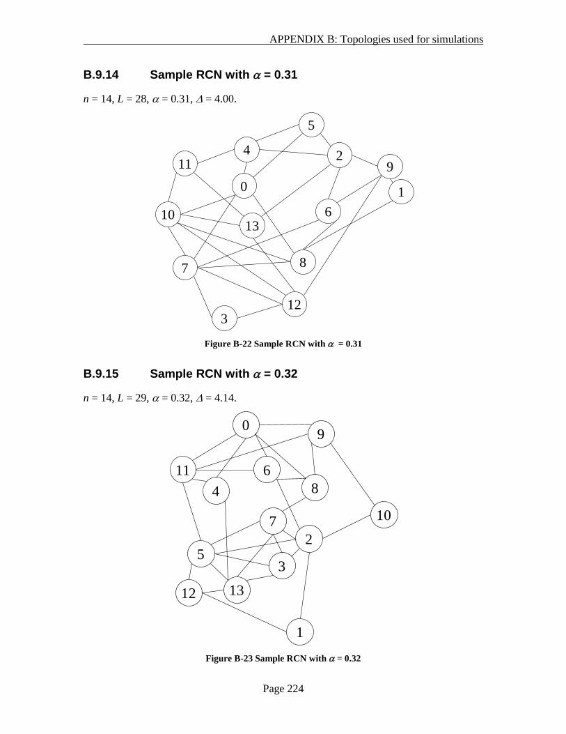
APPENDIX B: Topologies used for simulations
Page 224
B.9.14 Sample RCN with α = 0.31
n = 14, L = 28, α = 0.31, ∆ = 4.00.
0 1
2
3
4
5
6
7 8
9
10
11
12
13
Figure B-22 Sample RCN with α = 0.31
B.9.15 Sample RCN with α = 0.32
n = 14, L = 29, α = 0.32, ∆ = 4.14.
0
1
2
3
4
5
6
7
8
9
10
11
12 13
Figure B-23 Sample RCN with α = 0.32

APPENDIX B: Topologies used for simulations
Page 225
B.9.16 Sample RCN with α = 0.33
n = 14, L = 30, α = 0.33, ∆ = 4.29.
01
2
3
4
5
6
7
8
910
11
12
13 Figure B-24 Sample RCN with α = 0.33
B.9.17 Sample RCN with α = 0.34
n = 14, L = 31, α = 0.34, ∆ = 4.43.
0
1
2
3
4
5
6
7
8
9
10
11
12
13
Figure B-25 Sample RCN with α = 0.34

APPENDIX B: Topologies used for simulations
Page 226
B.9.18 Sample RCN with α = 0.35
n = 14, L = 32, α = 0.35, ∆ = 4.57.
0
1
23
4
5
6 7
8
9
10
1112
13
Figure B-26 Sample RCN with α = 0.35
B.9.19 RCN with α = 0.36
n = 14, L = 33, α = 0.36, ∆ = 4.71.
0
1
2
3
4
5
6
7
8
9
10
11
12
13
Figure B-27 RCN with α = 0.36

APPENDIX B: Topologies used for simulations
Page 227
B.10 Chapter references
[Myers 01] Alec Myers, “Architecture for Optical Burst Switching”, MRes Thesis 2001,
University College London.
[Baroni 96] S. Baroni, P. Bayvel, J. Midwinter, “Influence of physical connectivity on the
number of wavelengths in dense wavelength-routed optical networks”. Proc. Optical
Fiber Communication (OFC) Conf. 1996, pp. 25-26.
[Baroni 98] Stefano Baroni, “Routing and wavelength allocation in WDM optical
networks”. PhD thesis, May 1998. University College London.
[Zapata-Beghelli 06] Alejandra Zapata-Beghelli, “Resource allocation and scalability in
dynamic wavelength-routed optical networks”. PhD thesis, 2006. University College
London.

APPENDIX C: Value of agility detailed results
Page 228
Appendix C Value of agility detailed results This appendix provides the more detailed results referenced in section 3.4.7. Section
3.4.8 provides a summary.
0
0.0001
0.0002
0.0003
0.0004
0.0005
0.0006
0.0007
0.0008
0.0009
0.001
1 10 100 1000 10000
P(B)
Wavelength reallocation period
Load averaging 10 slots
Figure C-1 Load averaging 10 slots/demand
0
0.0005
0.001
0.0015
0.002
0.0025
0.003
0.0035
0.004
1 10 100 1000 10000
P(B)
Wavelength reallocation period
Load averaging 12 slots
Figure C-2 Load averaging 12 slots/demand

APPENDIX C: Value of agility detailed results
Page 229
0
0.002
0.004
0.006
0.008
0.01
0.012
1 10 100 1000 10000
P(B)
Wavelength reallocation period
Load averaging 14 slots
Figure C-3 Load averaging 14 slots/demand
0
0.005
0.01
0.015
0.02
0.025
1 10 100 1000 10000
P(B)
Wavelength reallocation period
Load averaging 16 slots
Figure C-4 Load averaging 16 slots/demand

APPENDIX C: Value of agility detailed results
Page 230
0
0.005
0.01
0.015
0.02
0.025
0.03
0.035
0.04
0.045
1 10 100 1000 10000
P(B)
Wavelength reallocation period
Load averaging 18 slots
Figure C-5 Load averaging 18 slots/demand
0
0.01
0.02
0.03
0.04
0.05
0.06
1 10 100 1000 10000
P(B)
Wavelength reallocation period
Load averaging 19 slots
Figure C-6 Load averaging 19 slots/demand
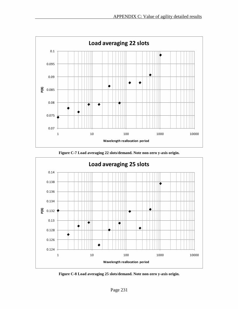
APPENDIX C: Value of agility detailed results
Page 231
0.07
0.075
0.08
0.085
0.09
0.095
0.1
1 10 100 1000 10000
P(B)
Wavelength reallocation period
Load averaging 22 slots
Figure C-7 Load averaging 22 slots/demand. Note non-zero y-axis origin.
0.124
0.126
0.128
0.13
0.132
0.134
0.136
0.138
0.14
1 10 100 1000 10000
P(B)
Wavelength reallocation period
Load averaging 25 slots
Figure C-8 Load averaging 25 slots/demand. Note non-zero y-axis origin.
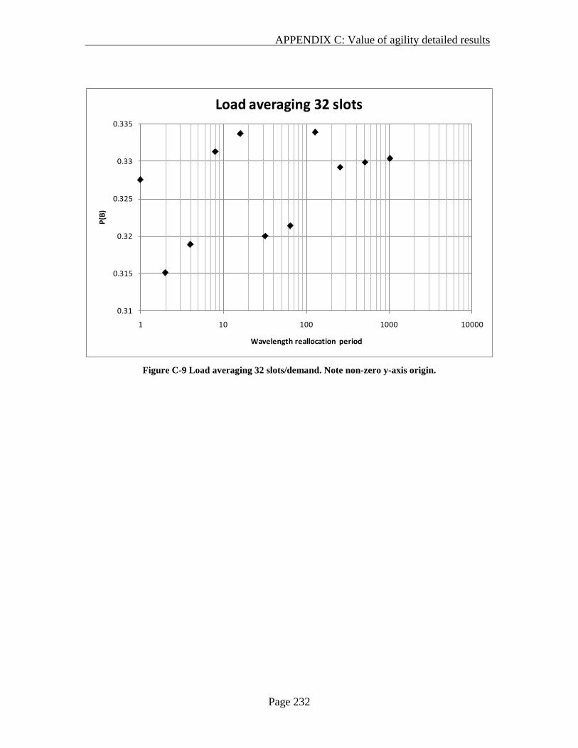
APPENDIX C: Value of agility detailed results
Page 232
0.31
0.315
0.32
0.325
0.33
0.335
1 10 100 1000 10000
P(B)
Wavelength reallocation period
Load averaging 32 slots
Figure C-9 Load averaging 32 slots/demand. Note non-zero y-axis origin.