1

Control System lab Experiments using Compose

(VTU University Syllabus)

Author: Sijo George

Reviewer: Sreeram Mohan

Altair Engineering, Bangalore

Version: 1

Date: 09/11/2016

2

CONTENTS

EXP. 1: STEP RESPONSE OF A SECOND ORDER SYSTEM ............................................................................. 3

EXP.1.B STEP RESPONSE OF A SECOND ORDER SYSTEM FOR VARIOUS VALUES OF ZETA ...................... 15

EXP.2 EFFECT OF P, PD, PI AND PID CONTROLLER ..................................................................................... 17

EXP.3 ROOT LOCUS, BODE AND NYQUIST PLOT ........................................................................................ 21

EXP.4 RELATION BETWEEN FREQUENCY RESPONSE AND TRANSIENT RESPONSE ................................... 29

TABLE OF FIGURES

FIGURE 1.a: STEP RESPONSE AND ADDITION OF ZERO TO THE GIVEN SYSTEM ................................. 144

FIGURE 1.b: STEP RESPONSE FOR DIFFERENT DAMPING RATIO OF A SECOND ORDER SYSTEM .......... 166

FIGURE 2.a: EFFECT P, PD, PI AND PID CONTROLLERS ........................................................................ 20

FIGURE 3.a: ROOT LOCUS AND EFFECT OF ADDING POLES AND

ZEROS………………………………………………165 FIGURE 3.b: BODE PLOT OF THE GIVEN

SYSTEM……………………………………………..………………………………...167 FIGURE 3.c: NYQUIST PLOT OF THE

GIVEN SYSTEM………………………………………..………………………………….28 FIGURE 4.a: BODE PLOT FOR

TRANSIENT AND FREQUENCY RESPONSE………………………………..…………….31 FIGURE 4.b: RESONANT

PEAK, MAX.OVERSHOOT AND DAMPING RATIO..……………………..…………………32 FIGURE 4.c:

BANDWIDTH AND DAMPING RATIO….…………………………………………………………..……………….32

3

EXP. 1: STEP RESPONSE OF A SECOND ORDER SYSTEM

Aim & Description:

(1)To determine the step response of a second order system and evaluation of time domain

specifications.

(2) To evaluate the effect of additional zeros on time response of second order system.

Step response is the time behavior of the outputs of a general system when its inputs change

from zero to one in a very short time.

2010

1)(

3

sssG

Software code:

clc; clear; close all;

sys.num = [1]; % Numerator

sys.den = [1 10 20]; % Denominator

sys1=tf(sys); % Finding transfer function

kp=dcgain(sys) % gain when frequency is zero(s=0)

ess=1/(1+kp) % Steady state error

w = sqrt (sys.den(3)) % Finding natural frequency

zeta = sys.den(2) / (2*w) % Damping ratio

TD=(1+0.7*zeta)/w % Delay time

TS = 4/ (zeta*w) % Settling time

TP = pi/ (w*sqrt(1-zeta^2)) % Peak Time

TR=(pi-atan((sqrt(1-zeta^2))/zeta))/(w*sqrt(1-zeta^2)) % Rise Time

Percentovershoot= exp(-zeta*pi/ sqrt(1-zeta^2))*100 % Overshoot

subplot(2,2,1)

[z,t]=step(sys); % Step response

plot(t,z);

title('Step response');

xlabel('Time (sec)');

4

ylabel('Amplitude');grid on;

subplot(2,2,2)

pzmap(sys.num,sys.den); % Pole zero plot

title('Pole zero map of the given system')

grid on;

%% Adding Zero to the given system

sys.num = conv(sys.num,[1 1]);

sys2=tf(sys)

[f,t]=step(sys);

subplot(2,2,3)

plot(t,f);

title('Step response after addition of zero')

xlabel('Time (sec)');

ylabel('Amplitude');grid on;

subplot(2,2,4)

pzmap(sys.num,sys.den) % Pole zero plot when zero is added

title('Pole zero map when zero is added')

grid on;

%----------------------Function created to display transfer function using string concept

function [sys]=tf(varargin)

if length(varargin)==1

sys=varargin{1};

b=sys.num;

a=sys.den;

end

if length(varargin)==2

b=varargin{1};

a=varargin{2};

end

5

[fopen_fileID] = fopen('testfile.txt', 'w'); %open a text file

l=length(b); % Number of numerator coefficients

m=length(a); % Number of denominator coefficients

%%%%-----------Numerator

if length(b)==1 % Check the numerator has only one coefficient

fprintf(fopen_fileID, ' %g\n',b(1)); % Print numerator

fprintf(fopen_fileID,' %s','-----------'); % to draw the separation b/w numerator and denominator

end

if length(b)==2 % Check the numerator has two coefficients

c{1}=sprintf('%g%s',b(1),'s'); % store first numerator coefficient in a cell 'c{1}'

c{2}=b(end); % store second numerator coefficient in a cell 'c{2}'

fprintf(fopen_fileID, '%s',c{1}); % print numerator

if b(end)>0

fprintf(fopen_fileID, '%s','+'); % to print + sign before the last coefficient if it is positive

end

fprintf(fopen_fileID, '%g\n',c{end});

fprintf(fopen_fileID,' %s','-----------'); % to draw the separation b/w numerator and denominator

end

if length(b)>2 % Check the numerator has more than two coefficients

i=l-1; % Initializing value of i to print the exponential term

for k=1:l-2 % Loop defined for the numerator coefficients excluding the last and second last

coefficient

h=sprintf('%g%s%g',b(k),'s^',i); % Print numerator coefficient and storing to the variable 'h'

c{k}=h; %store the numerator coefficient in a cell 'c'

i=i-1; % Decrementing the power of i for printing the exponential terms in the correct way

end

c{k+1}=sprintf('%g%s',b(k+1),'s'); % store the second last coefficient in 'c'

c{k+2}=b(end); % store last coefficient in 'c'

c;

6

for t=1:length(c)-1

fprintf(fopen_fileID, '%s',c{t}); % Print the numerator coefficients except the last coefficient of the

transfer function

R=cell2mat(c(t+1));

T=strcmp(R(1),'-'); %returns 1 if the comparison matches

if (t~=(length(c)-1))

if T==0

fprintf(fopen_fileID, '%s','+'); %to print + sign if the next coefficient is positive except the last digit

end

end

end

if b(end)>0

fprintf(fopen_fileID, '%s','+'); %To print + sign before it when the last coefficient is positive

end

fprintf(fopen_fileID,'%g\n',c{end}); % Print the last numerator coefficient of the transfer function

fprintf(fopen_fileID,' %s','-----------');

end

%------------Denominator

if length(a)==1 % Check if the denominator has only one coefficient

fprintf(fopen_fileID, '\n %g\n',a(1));

end

if length(a)==2 % Check if the denominator has two coefficients

f{1}=sprintf('\n %g%s',a(1),'s');

f{2}=a(end);

fprintf(fopen_fileID, '%s',f{1}); % print denominator

if a(end)>0

fprintf(fopen_fileID, '%s','+'); %to print + sign before the last coefficient it is positive

end

fprintf(fopen_fileID, '%g\n',f{end}); %print the last coefficient

7

end

if length(a)>2 %Check if the length of denominator has more than 2 coefficients

j=m-1;

for g=1:m-2

e=sprintf('%g%s%g',a(g),'s^',j); % storing ‘s’ terms and its coefficient power in a variable

f{g}=e; %assigning to a cell

j=j-1;

end

f{g+1}=sprintf('%g%s',a(g+1),'s');

f{g+2}=a(end);

fprintf(fopen_fileID, '\n %s',f{1}); %to print the first coefficient of denominator along with the ‘s’

term

R2=cell2mat(f(2));

T2=strcmp(R2(1),'-'); %returns 1 if the comparison matches

if T2==0

fprintf(fopen_fileID, '%s','+'); %To print + sign before second term if it is a positive

end

for u=2:length(f)-1

fprintf(fopen_fileID, '%s',f{u}); % to print the coefficients from second to last

R1=cell2mat(f(u+1)); %converting cell to matrix

T1=strcmp(R1(1),'-'); % gives 1 as output if the comparison matches

if (u~=(length(f)-1))

if T1==0

fprintf(fopen_fileID, '%s','+'); %to print the + sign if the next coefficient is positive

end

end

end

if a(end)>0

fprintf(fopen_fileID, '%s','+'); %to print + sign if the last coefficient is positive

8

end

end

fprintf(fopen_fileID, '%g\n',f{end}); %to print the last coefficient

fclose(fopen_fileID);

content = type('testfile.txt');

sys=content{1,1} ;

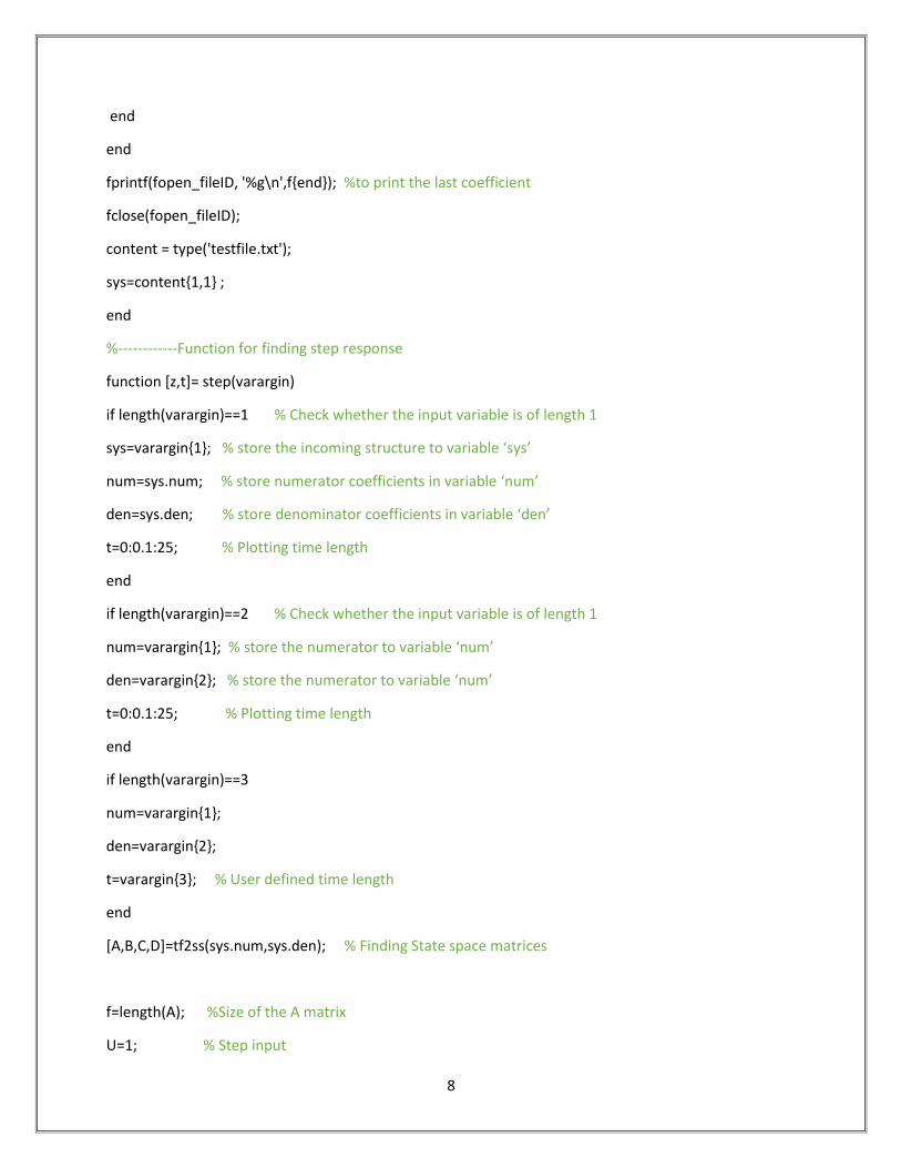
end

%------------Function for finding step response

function [z,t]= step(varargin)

if length(varargin)==1 % Check whether the input variable is of length 1

sys=varargin{1}; % store the incoming structure to variable ‘sys’

num=sys.num; % store numerator coefficients in variable ‘num’

den=sys.den; % store denominator coefficients in variable ‘den’

t=0:0.1:25; % Plotting time length

end

if length(varargin)==2 % Check whether the input variable is of length 1

num=varargin{1}; % store the numerator to variable ‘num’

den=varargin{2}; % store the numerator to variable ‘num’

t=0:0.1:25; % Plotting time length

end

if length(varargin)==3

num=varargin{1};

den=varargin{2};

t=varargin{3}; % User defined time length

end

[A,B,C,D]=tf2ss(sys.num,sys.den); % Finding State space matrices

f=length(A); %Size of the A matrix

U=1; % Step input

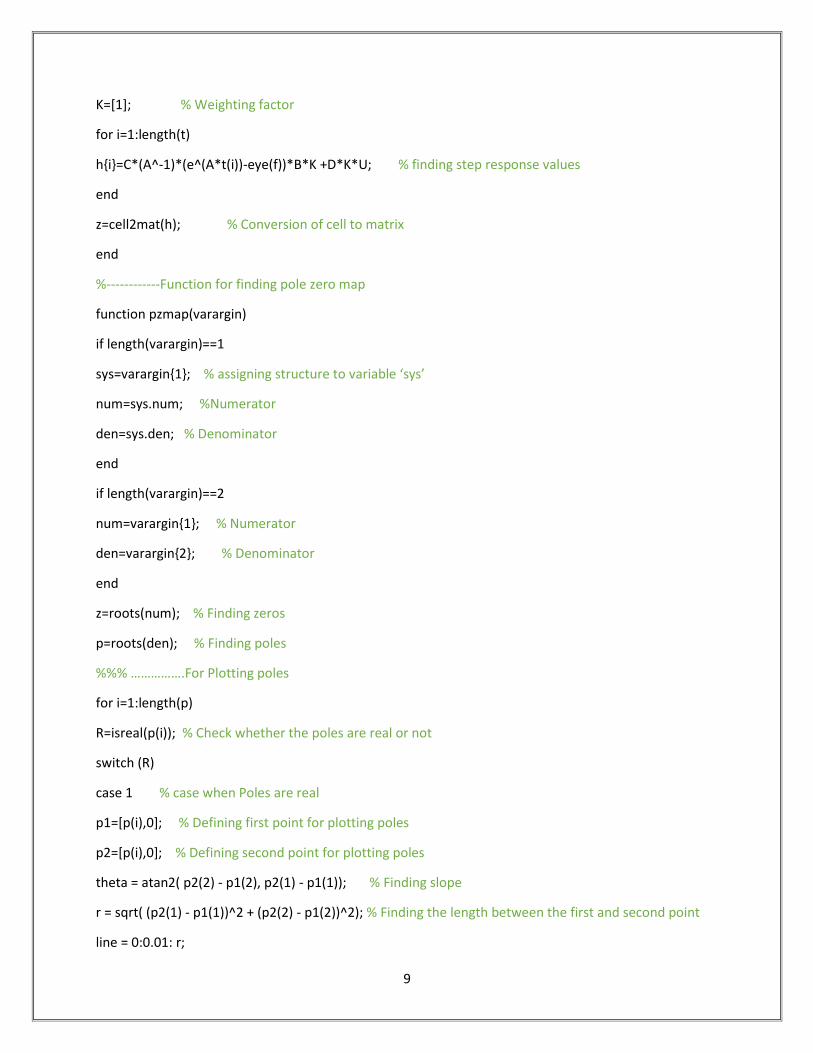
9

K=[1]; % Weighting factor

for i=1:length(t)

h{i}=C*(A^-1)*(e^(A*t(i))-eye(f))*B*K +D*K*U; % finding step response values

end

z=cell2mat(h); % Conversion of cell to matrix

end

%------------Function for finding pole zero map

function pzmap(varargin)

if length(varargin)==1

sys=varargin{1}; % assigning structure to variable ‘sys’

num=sys.num; %Numerator

den=sys.den; % Denominator

end

if length(varargin)==2

num=varargin{1}; % Numerator

den=varargin{2}; % Denominator

end

z=roots(num); % Finding zeros

p=roots(den); % Finding poles

%%% …………….For Plotting poles

for i=1:length(p)

R=isreal(p(i)); % Check whether the poles are real or not

switch (R)

case 1 % case when Poles are real

p1=[p(i),0]; % Defining first point for plotting poles

p2=[p(i),0]; % Defining second point for plotting poles

theta = atan2( p2(2) - p1(2), p2(1) - p1(1)); % Finding slope

r = sqrt( (p2(1) - p1(1))^2 + (p2(2) - p1(2))^2); % Finding the length between the first and second point

line = 0:0.01: r;

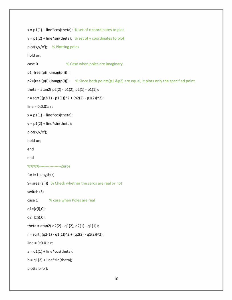
10

x = p1(1) + line*cos(theta); % set of x coordinates to plot

y = p1(2) + line*sin(theta); % set of y coordinates to plot

plot(x,y,'x'); % Plotting poles

hold on;

case 0 % Case when poles are imaginary.

p1=[real(p(i)),imag(p(i))];

p2=[real(p(i)),imag(p(i))]; % Since both points(p1 &p2) are equal, it plots only the specified point

theta = atan2( p2(2) - p1(2), p2(1) - p1(1));

r = sqrt( (p2(1) - p1(1))^2 + (p2(2) - p1(2))^2);

line = 0:0.01: r;

x = p1(1) + line*cos(theta);

y = p1(2) + line*sin(theta);

plot(x,y,'x');

hold on;

end

end

%%%%-----------------Zeros

for i=1:length(z)

S=isreal(z(i)) % Check whether the zeros are real or not

switch (S)

case 1 % case when Poles are real

q1=[z(i),0];

q2=[z(i),0];

theta = atan2( q2(2) - q1(2), q2(1) - q1(1));

r = sqrt( (q2(1) - q1(1))^2 + (q2(2) - q1(2))^2);

line = 0:0.01: r;

a = q1(1) + line*cos(theta);

b = q1(2) + line*sin(theta);

plot(a,b,'o');

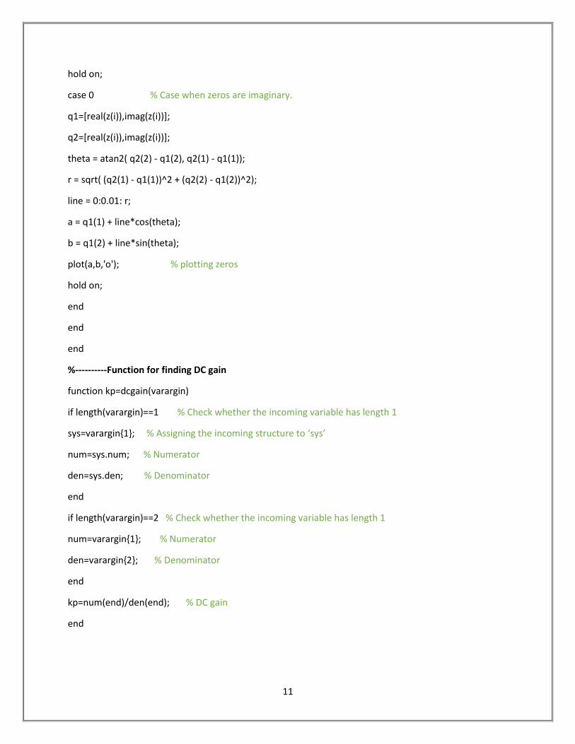
11

hold on;

case 0 % Case when zeros are imaginary.

q1=[real(z(i)),imag(z(i))];

q2=[real(z(i)),imag(z(i))];

theta = atan2( q2(2) - q1(2), q2(1) - q1(1));

r = sqrt( (q2(1) - q1(1))^2 + (q2(2) - q1(2))^2);

line = 0:0.01: r;

a = q1(1) + line*cos(theta);

b = q1(2) + line*sin(theta);

plot(a,b,'o'); % plotting zeros

hold on;

end

end

end

%----------Function for finding DC gain

function kp=dcgain(varargin)

if length(varargin)==1 % Check whether the incoming variable has length 1

sys=varargin{1}; % Assigning the incoming structure to ‘sys’

num=sys.num; % Numerator

den=sys.den; % Denominator

end

if length(varargin)==2 % Check whether the incoming variable has length 1

num=varargin{1}; % Numerator

den=varargin{2}; % Denominator

end

kp=num(end)/den(end); % DC gain

end

12

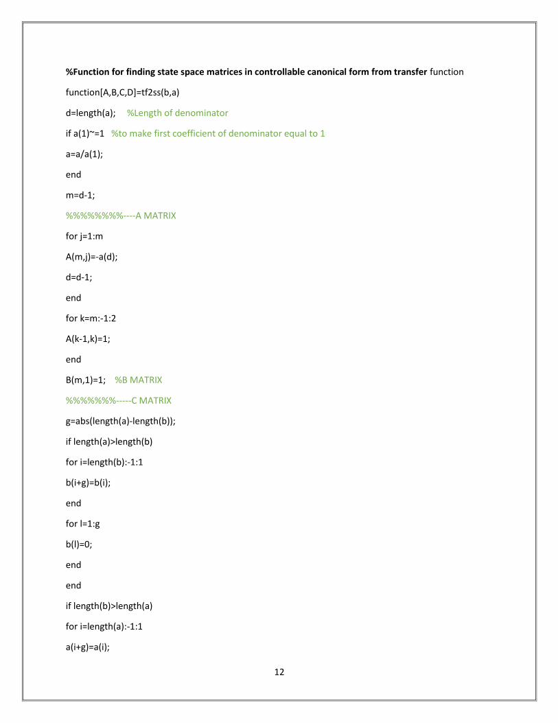
%Function for finding state space matrices in controllable canonical form from transfer function

function[A,B,C,D]=tf2ss(b,a)

d=length(a); %Length of denominator

if a(1)~=1 %to make first coefficient of denominator equal to 1

a=a/a(1);

end

m=d-1;

%%%%%%%%----A MATRIX

for j=1:m

A(m,j)=-a(d);

d=d-1;

end

for k=m:-1:2

A(k-1,k)=1;

end

B(m,1)=1; %B MATRIX

%%%%%%%-----C MATRIX

g=abs(length(a)-length(b));

if length(a)>length(b)

for i=length(b):-1:1

b(i+g)=b(i);

end

for l=1:g

b(l)=0;

end

end

if length(b)>length(a)

for i=length(a):-1:1

a(i+g)=a(i);

13

end

for l=1:g

a(l)=0;

end

end

b

f=m;

for p=2:1:m+1

C(1,f)=b(p)-a(p)*b(1);

f=f-1;

end

D=b(1); %D MATRIX

end

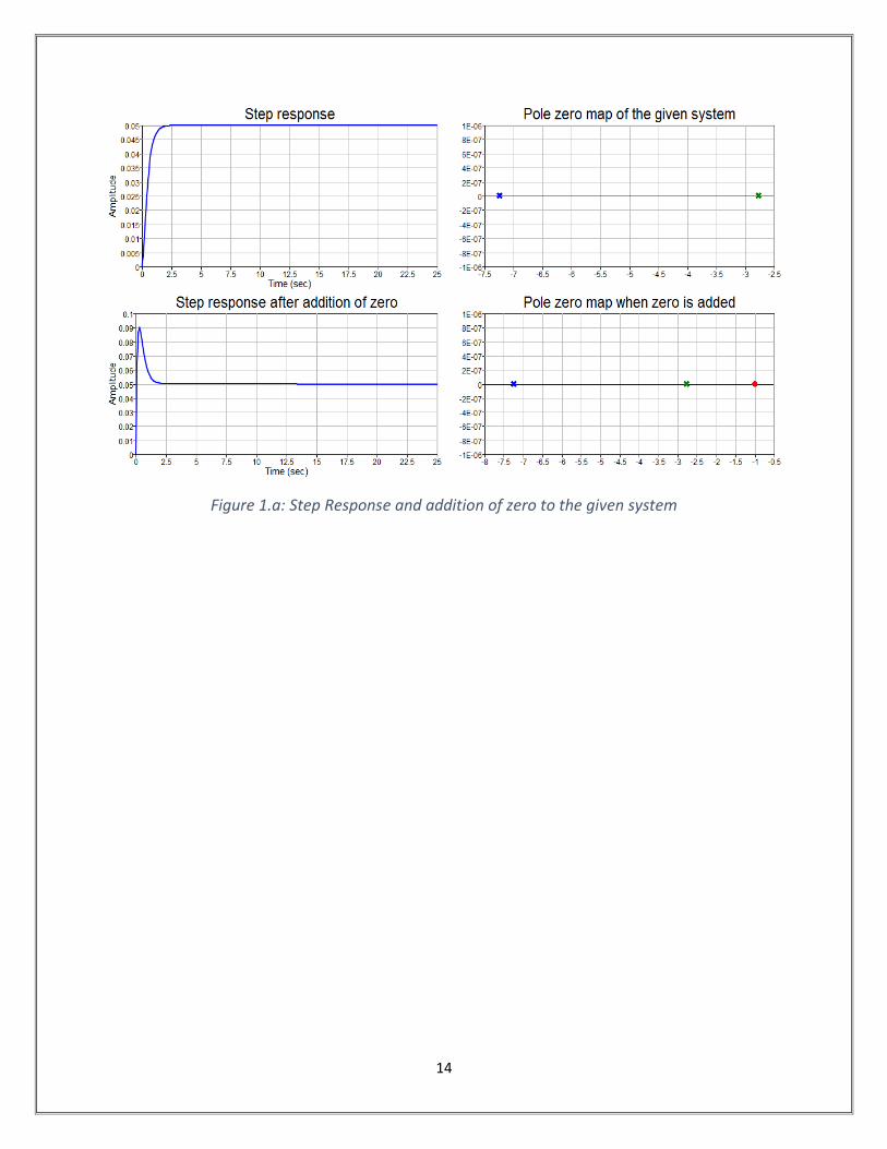
Simulation Results:

sys1 = 1 --------------

1s^2+10s+20

sys2 = 1s+1 ------------- 1s^2+10s+20

kp = 0.05 ( DC gain) ess = 0.952380952 ( Steady state error) w = 4.47213595 (Natural frequency) zeta = 1.11803399 (Damping ratio) TD = 0.398606798 (Delay time) TS = 0.8 (Settling Time) TP = 0 - 1.40496295i (Peak Time) TR = -0.21520447 - 1.40496295i (Rise Time) Percent overshoot = 73.7368878 + 67.5490294i (Percent Overshoot)

14

Figure 1.a: Step Response and addition of zero to the given system

15

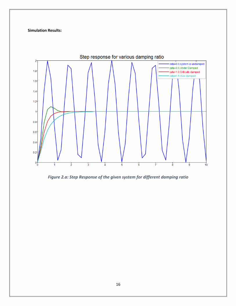
EXP.1.B STEP RESPONSE OF A SECOND ORDER SYSTEM FOR VARIOUS

VALUES OF ZETA

Description: Damping ratio is a dimensionless measure describing how oscillations in a system decay

after a disturbance. Many systems exhibit oscillatory behavior when they are disturbed from their position

of static equilibrium.

Software Code:

clc; close all; clear

zeta=[0 0.6 1 1.5]; % Various damping ratio

t=0:0.2:10; % Plotting time length

num=[0 0 25]; % Numerator

den1=[1 10*zeta(1) 25];

den2=[1 10*zeta(2) 25];

den3=[1 10*zeta(3) 25];

den4=[1 10*zeta(4) 25];

figure(1)

[f1,t]=step(num,den1,t);plot(t,f1);hold on; % Step Response

[f2,t]=step(num,den2,t);plot(t,f2);hold on;

[f3,t]=step(num,den3,t);plot(t,f3);hold on;

[f4,t]=step(num,den4,t);plot(t,f4);hold on;

legend('zeta=0.0,system is undamped','zeta=0.6,Under Damped','zeta=1.0,Critically

damped','zeta=1.5,Over damped')

title('Step response for various values of zeta')

16

Simulation Results:

Figure 2.a: Step Response of the given system for different damping ratio

17

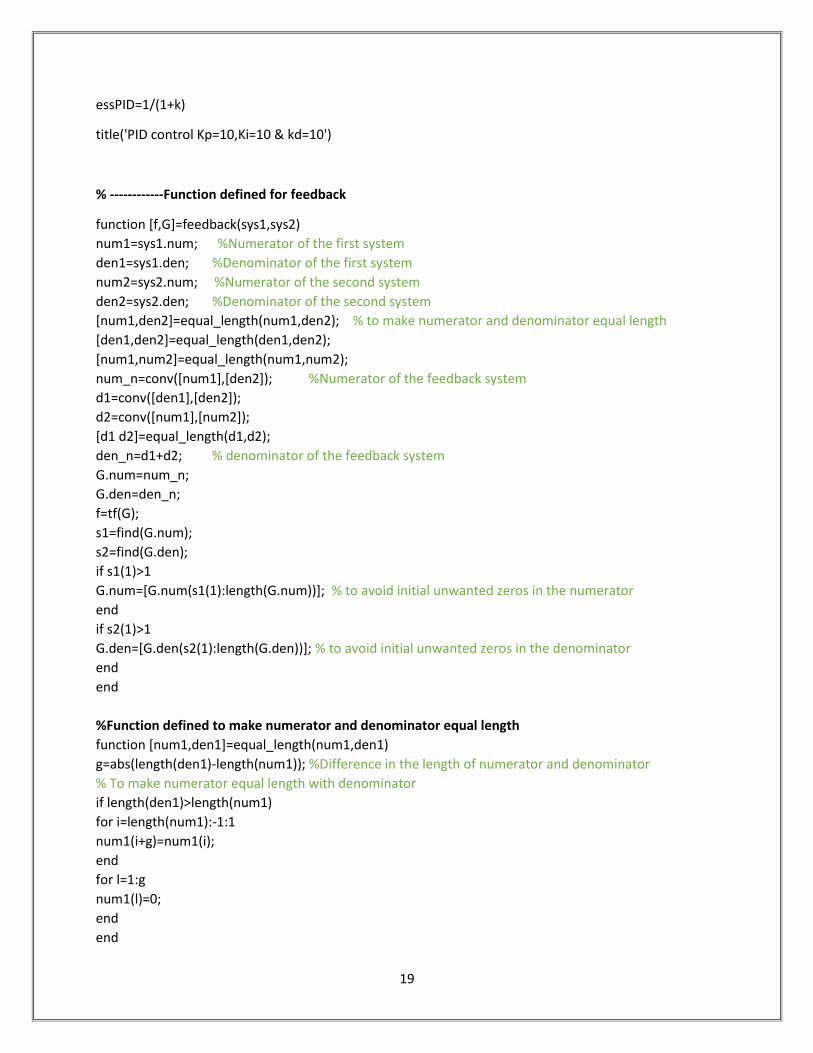
EXP.2 EFFECT OF P, PD, PI AND PID CONTROLLER

Aim & Description: To obtain step response of the given system and evaluate the effect P,PD,PI and PID controllers.

A controller is a device, historically using mechanical, hydraulic, pneumatic or electronic techniques often

in combination, but more recently in the form of a microprocessor or computer, which monitors and

physically alters the operating conditions of a given dynamical system.

415.0

1)(

3

sssG

Software Code:

clc; clear; close all;

sys.num=[1]; % Numerator of the system is defined as a structure

sys.den=[0.5 1 4]; % Denominator of the system is defined as a structure

sys1=tf(sys) % Print transfer function and store it in sys1.

sys5.num=[1]; %Numerator of unity feedback system

sys5.den=[1]; %Denominator of unity feedback system

[f,G]=feedback(sys,sys5) % Gives transfer function of the system with unity feedback

[z,t]=step(G); % Step response of the system

subplot(2,3,1);plot(t,z);grid on;

title('Step response of given system');

%Proportional controller

kp=10;

sys.num=kp*sys.num; % Numerator augmented with P controller

sys2=tf(sys);

[f,G]=feedback(sys,sys5)

[z,t]=step(G);

subplot(2,3,2);

plot(t,z);grid on;

title('Proportional contol Kp=10')

k=dcgain(sys) % DC gain of the system ( s=0)

18

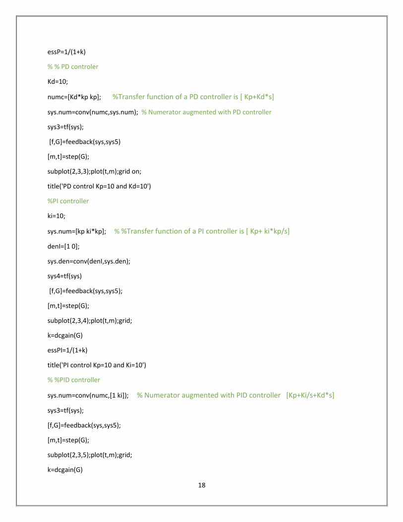
essP=1/(1+k)

% % PD controler

Kd=10;

numc=[Kd*kp kp]; %Transfer function of a PD controller is [ Kp+Kd*s]

sys.num=conv(numc,sys.num); % Numerator augmented with PD controller

sys3=tf(sys);

[f,G]=feedback(sys,sys5)

[m,t]=step(G);

subplot(2,3,3);plot(t,m);grid on;

title('PD control Kp=10 and Kd=10')

%PI controller

ki=10;

sys.num=[kp ki*kp]; % %Transfer function of a PI controller is [ Kp+ ki*kp/s]

denI=[1 0];

sys.den=conv(denI,sys.den);

sys4=tf(sys)

[f,G]=feedback(sys,sys5);

[m,t]=step(G);

subplot(2,3,4);plot(t,m);grid;

k=dcgain(G)

essPI=1/(1+k)

title('PI control Kp=10 and Ki=10')

% %PID controller

sys.num=conv(numc,[1 ki]); % Numerator augmented with PID controller [Kp+Ki/s+Kd*s]

sys3=tf(sys);

[f,G]=feedback(sys,sys5);

[m,t]=step(G);

subplot(2,3,5);plot(t,m);grid;

k=dcgain(G)

19

essPID=1/(1+k)

title('PID control Kp=10,Ki=10 & kd=10')

% ------------Function defined for feedback

function [f,G]=feedback(sys1,sys2)

num1=sys1.num; %Numerator of the first system

den1=sys1.den; %Denominator of the first system

num2=sys2.num; %Numerator of the second system

den2=sys2.den; %Denominator of the second system

[num1,den2]=equal_length(num1,den2); % to make numerator and denominator equal length

[den1,den2]=equal_length(den1,den2);

[num1,num2]=equal_length(num1,num2);

num_n=conv([num1],[den2]); %Numerator of the feedback system

d1=conv([den1],[den2]);

d2=conv([num1],[num2]);

[d1 d2]=equal_length(d1,d2);

den_n=d1+d2; % denominator of the feedback system

G.num=num_n;

G.den=den_n;

f=tf(G);

s1=find(G.num);

s2=find(G.den);

if s1(1)>1

G.num=[G.num(s1(1):length(G.num))]; % to avoid initial unwanted zeros in the numerator

end

if s2(1)>1

G.den=[G.den(s2(1):length(G.den))]; % to avoid initial unwanted zeros in the denominator

end

end

%Function defined to make numerator and denominator equal length

function [num1,den1]=equal_length(num1,den1)

g=abs(length(den1)-length(num1)); %Difference in the length of numerator and denominator

% To make numerator equal length with denominator

if length(den1)>length(num1)

for i=length(num1):-1:1

num1(i+g)=num1(i);

end

for l=1:g

num1(l)=0;

end

end

20

% To make denominator equal length with numerator

if length(num1)>length(den1)

for i=length(den1):-1:1

den1(i+g)=den1(i);

end

for l=1:g

den1(l)=0;

end

end

num1;

den1;

end

Simulation Results:

Figure 2.a: Effect of P, PD, PI and PID controllers

21

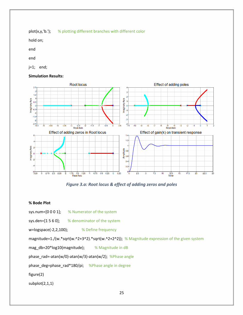
EXP.3 ROOT LOCUS, BODE AND NYQUIST PLOT

Aim & Description: 1) To sketch the root locus for the given transfer function 2) To sketch the nyquist plots for the given transfer function 3) To sketch the bode plots for the given transfer function

Root locus analysis is a graphical method for examining how the roots of a system change with

variation of a certain system parameter, commonly a gain within a feedback system.

Nyquist plot is a representation of the vector response of a feedback system (especially an amplifier) as a complex graphical plot showing the relationship between feedback and gain.

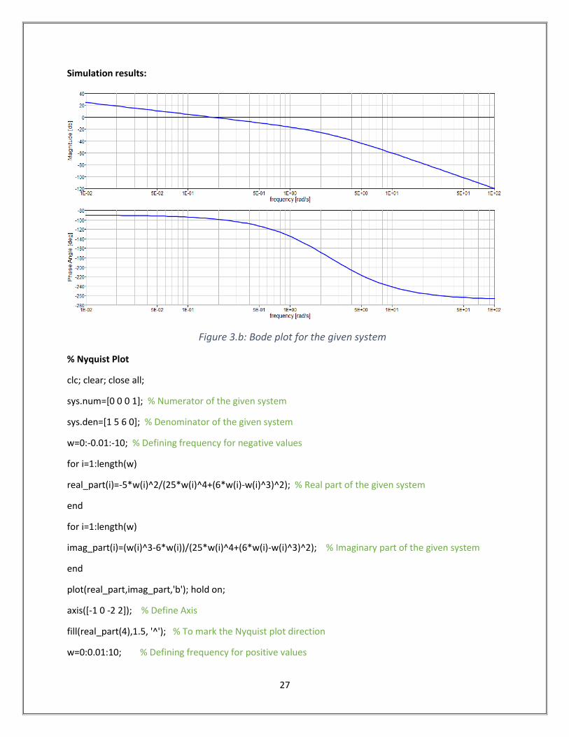
Bode plot is a graph of the frequency response of a system. It is usually a combination of a Bode

magnitude plot, expressing the magnitude (usually in decibels) of the frequency response, and a Bode phase plot, expressing the phase shift. Both quantities are plotted against a horizontal axis proportional to the logarithm of frequency.

065

1)(

23

ssssG

Software Code:

clc; clear; close all;

sys.num=[0 0 0 1]; % Numerator of the system

sys.den=[1 5 6 0]; % Denominator of the system

sys1=tf(sys); % Printing transfer function

subplot(2,2,1)

rlocus(sys); % root locus of the system

title('Root locus'); ylabel('Imaginary Axis')

% %Effect of adding poles

sys.den=conv([1 10],sys.den); % Adding poles to the denominator

sys2=tf(sys);

subplot(2,2,2)

rlocus(sys); % root locus of the system when extra poles are added

title(' Effect of adding poles');ylabel('Imaginary Axis')

% %Effect of adding zeros

22

sys.num=conv([1 1],sys.num); % Adding zeros to the denominator

sys.den=[1 5 6 0];

sys3=tf(sys);

subplot(2,2,3)

rlocus(sys); % root locus of the system when poles are added

title(' Effect of adding zeros in Root locus');ylabel('Imaginary Axis')

% % effect of k on the transient response

k=10;

t=0:0.01:20;

G.num=[0 0 0 k]

G.den=[1 5 6 k];

[z,t]=step(G); % Finding step response of the system

subplot(2,2,4);xlabel('Time');ylabel('Amplitude')

plot(t,z); grid on;

title('Effect of k on transient response');

%-------------Function defined for rlocus

function rlocus(sys)

num=sys.num;

den=sys.den;

%%---------To make numerator and denominator equal length

g=abs(length(den)-length(num));

if length(den)>length(num) % If denominator length is greater than numerator length

for i=length(num):-1:1

num(i+g)=num(i); % shifting numerator coefficients to the right

end

for l=1:g

num(l)=0; % Appending zeros to the index where numerator coefficients originally existed

end

end

23

if length(num)>length(den) % If numerator length is greater than denominator length

for i=length(den):-1:1

den(i+g)=den(i); % shifting denominator coefficients to the right

end

for l=1:g

den(l)=0; % Appending zeros to the index where denominator coefficients originally existed

end

end

%%%-------------------------

d=roots(den); % Finding poles

n=roots(num); % Finding zeros

P=length(d); % Number of poles

Z=length(n); % Number of zeros

pzmap(num,den); % P-Z map of the given system

grid on;hold on;

i = 1;

for k=0:0.1:30

r3=den+k*num; % Denominator of unity feedback system for various gain values

r2{i}=roots(r3); % poles of the feedback system

i = i+1;

end

if P==4 && Z==0 % Special case for no zeros and 4 poles

for k=0:5:1000

r3=den+k*num;

r2{i}=roots(r3);

i = i+1;

end

end

z2=cell2mat(r2); % Conversion of cell to matrix

24

%---------Extraction of values from the matrix

j=1;

for k=1:length(d)

for i=P+k:length(d):numel(z2)

b(j)=z2(i);

j=j+1;

end

%------Plotting the extracted values

for i=1:numel(b)

p1=[real(b(i)),imag(b(i))]; % Define the first point to plot the root locus

p2=[real(b(i)),imag(b(i))]; % Define the second point to plot the root locus

theta = atan2( p2(2) - p1(2), p2(1) - p1(1)); %Define slope

r = sqrt( (p2(1) - p1(1))^2 + (p2(2) - p1(2))^2); % Distance between first and second point

line = 0:0.01: r;

x = p1(1) + line*cos(theta); % set of x coordinates to plot root locus

y = p1(2) + line*sin(theta); % set of y coordinates to plot root locus

if k==1

plot(x,y,'cyan.'); % plotting different branches with different color

hold on;

end

if k==2

plot(x,y,'g.'); % plotting different branches with different color

hold on;

end

if k==3

plot(x,y,'r.'); % plotting different branches with different color

hold on;

end

if k==4

25

plot(x,y,'b.'); % plotting different branches with different color

hold on;

end

end

j=1; end;

Simulation Results:

Figure 3.a: Root locus & effect of adding zeros and poles

% Bode Plot

sys.num=[0 0 0 1]; % Numerator of the system

sys.den=[1 5 6 0]; % denominator of the system

w=logspace(-2,2,100); % Define frequency

magnitude=1./(w.*sqrt(w.^2+3^2).*sqrt(w.^2+2^2)); % Magnitude expression of the given system

mag_db=20*log10(magnitude); % Magnitude in dB

phase_rad=-atan(w/0)-atan(w/3)-atan(w/2); %Phase angle

phase_deg=phase_rad*180/pi; %Phase angle in degree

figure(2)

subplot(2,1,1)

26

semilogx(w,mag_db) % Magnitude plot in semilog graph

xlabel('frequency [rad/s]'),ylabel('Magnitude [db]'),grid on;

subplot(2,1,2)

semilogx(w,phase_deg) % Phase plot

xlabel('frequency [rad/s]'),ylabel('Phase Angle [deg]'),grid on;

%%--------Gain Margin

[wgc,fval] = fsolve(@func,5) % gain crossover frequency

gm=1./(wgc.*sqrt(wgc.^2+3^2).*sqrt(wgc.^2+2^2)) % Gain Margin

%--------Phase margin

j=1;

for i=1:length(mag_db)

if mag_db(i)>-0.2 && mag_db(i)<0.2 % setting a limit for finding wpm

b(j)=(i);

j=j+1;

end

end

wpm=min(w(b)) % phase crossover frequency

pm=(-atan(wpm/0)-atan(wpm/3)-atan(wpm/2))*180/pi+180 % Phase margin

%---------Function defined for solving gain crossover frequency

function w= func(w)

f=-atan(w/0)-atan(w/3)-atan(w/2)+180;

end

27

Simulation results:

Figure 3.b: Bode plot for the given system

% Nyquist Plot

clc; clear; close all;

sys.num=[0 0 0 1]; % Numerator of the given system

sys.den=[1 5 6 0]; % Denominator of the given system

w=0:-0.01:-10; % Defining frequency for negative values

for i=1:length(w)

real_part(i)=-5*w(i)^2/(25*w(i)^4+(6*w(i)-w(i)^3)^2); % Real part of the given system

end

for i=1:length(w)

imag_part(i)=(w(i)^3-6*w(i))/(25*w(i)^4+(6*w(i)-w(i)^3)^2); % Imaginary part of the given system

end

plot(real_part,imag_part,'b'); hold on;

axis([-1 0 -2 2]); % Define Axis

fill(real_part(4),1.5, '^'); % To mark the Nyquist plot direction

w=0:0.01:10; % Defining frequency for positive values

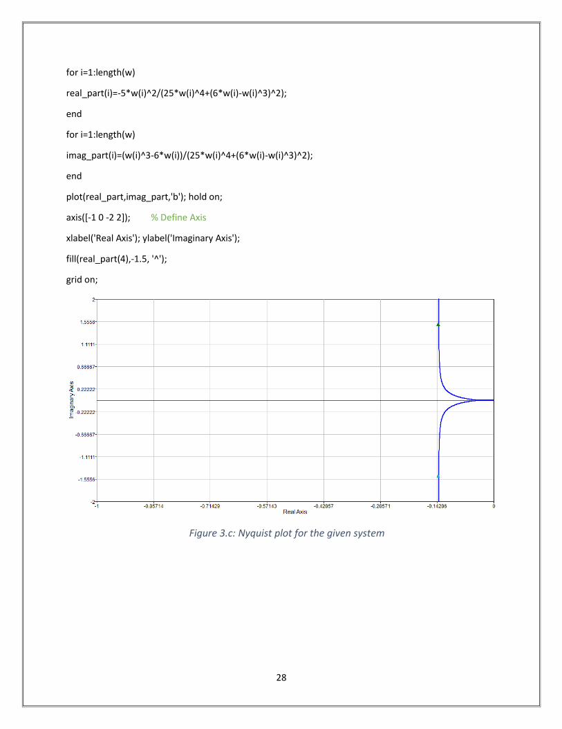
28

for i=1:length(w)

real_part(i)=-5*w(i)^2/(25*w(i)^4+(6*w(i)-w(i)^3)^2);

end

for i=1:length(w)

imag_part(i)=(w(i)^3-6*w(i))/(25*w(i)^4+(6*w(i)-w(i)^3)^2);

end

plot(real_part,imag_part,'b'); hold on;

axis([-1 0 -2 2]); % Define Axis

xlabel('Real Axis'); ylabel('Imaginary Axis');

fill(real_part(4),-1.5, '^');

grid on;

Figure 3.c: Nyquist plot for the given system

29

EXP.4 RELATION BETWEEN FREQUENCY RESPONSE AND TRANSIENT

RESPONSE

Aim & Description: To obtain the relation between frequency response and transient response

Transient response or natural response is the response of a system to a change from an

equilibrium or a steady state.

Frequency response is the quantitative measure of the output spectrum of a system or device in

response to a stimulus, and is used to characterize the dynamics of the system. It is a measure of

magnitude and phase of the output as a function of frequency, in comparison to the input.

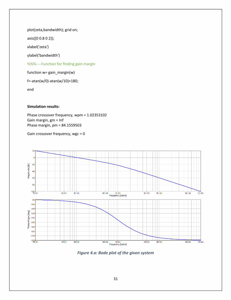
Software Code:

clc; clear; close all;

zeta=0:0.01:0.8; % Different damping ratio values

num=[1]; % Numerator

den=conv([1 0],[0.1 1]) % Denominator

g=tf(num,den);

w=logspace(-1,3,100); % Frequency range in log scale

magnitude=10./(w.*sqrt(w.^2+10^2)); % Magnitude expression

mag_db=20*log10(magnitude); % Magnitude expression in decibel

phase_rad=-atan(w/0)-atan(w/10); % Phase angle expression in radian

phase_deg=phase_rad*180/pi; % Phase angle expression in degree

figure(1)

subplot(2,1,1)

semilogx(w,mag_db) % Magnitude plot in semilog graph

xlabel('frequency [rad/s]'),ylabel('Magnitude [db]'),grid on;

subplot(2,1,2)

semilogx(w,phase_deg) % Phase plot in semi log graph

xlabel('frequency [rad/s]'),ylabel('Phase Angle [deg]'),grid on;

%% ---------Gain Margin

[wgc,fval] = fsolve(@gain_margin,5)

gm=1./(wgc.*sqrt(wgc.^2+10^2)) %---Gain margin

30

%--------Phase margin

j=1;

for i=1:length(mag_db)

if mag_db(i)>-0.25 && mag_db(i)<0.25 % Selection criteria for finding the index of corresponding 0db

frequency

b(j)=(i);

j=j+1;

end

end

wpm=min(w(b)) % phase crossover frequency

pm=(-atan(wpm/0)-atan(wpm/10))*180/pi+180 %---Phase margin

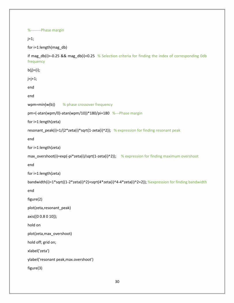
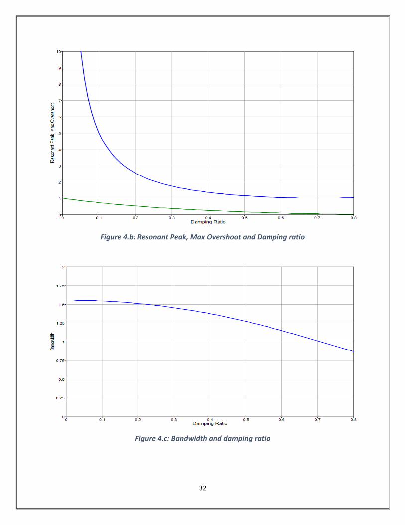
for i=1:length(zeta)

resonant_peak(i)=1/(2*zeta(i)*sqrt(1-zeta(i)^2)); % expression for finding resonant peak

end

for i=1:length(zeta)

max_overshoot(i)=exp(-pi*zeta(i)/sqrt(1-zeta(i)^2)); % expression for finding maximum overshoot

end

for i=1:length(zeta)

bandwidth(i)=1*sqrt((1-2*zeta(i)^2)+sqrt(4*zeta(i)^4-4*zeta(i)^2+2)); %expression for finding bandwidth

end

figure(2)

plot(zeta,resonant_peak)

axis([0 0.8 0 10]);

hold on

plot(zeta,max_overshoot)

hold off; grid on;

xlabel('zeta')

ylabel('resonant peak,max.overshoot')

figure(3)

31

plot(zeta,bandwidth); grid on;

axis([0 0.8 0 2]);

xlabel('zeta')

ylabel('bandwidth')

%%%----Function for finding gain margin

function w= gain_margin(w)

f=-atan(w/0)-atan(w/10)+180;

end

Simulation results:

Phase crossover frequency, wpm = 1.02353102 Gain margin, gm = Inf Phase margin, pm = 84.1559503

Gain crossover frequency, wgc = 0

Figure 4.a: Bode plot of the given system

32

Figure 4.b: Resonant Peak, Max Overshoot and Damping ratio

Figure 4.c: Bandwidth and damping ratio