control systems...disadvantages of open loop control system • disadvantages: – inaccurate and...
TRANSCRIPT
Control Systems

UNIT - I
CONTROL SYSTEM MODELLING
Overview
• We will learn about :– what are control systems and its types. – What is a block diagram and how to represent the
transfer function from the block diagrams.– What is Signal Flow Graph and how to obtain
transfer function.– How to solve block diagram problems and signal
flow graph problems.

Control Systems• A control system consisting of interconnected components is designed to
achieve a desired purpose. To understand the purpose of a control system, it is useful to examine examples of control systems through the course of history. These early systems incorporated many of the same ideas of feedback that are in use today.
• Modern control engineering practice includes the use of control design strategies for improving manufacturing processes, the efficiency of energy use, advanced automobile control, including rapid transit, among others.
• We also discuss the notion of a design gap. The gap exists between the complex physical system under investigation and the model used in the control system synthesis.
• The iterative nature of design allows us to handle the design gap effectively while accomplishing necessary tradeoffs in complexity, performance, and cost in order to meet the design specifications.
•

Introduction
System – An interconnection of elements and devices for a desired purpose.
Control System – An interconnection of components forming a system configuration that will provide a desired response.
Process – The device, plant, or system under control. The input and output relationship represents the cause-and-effect relationship of the process.

Introduction
Multivariable Control System
Open-Loop Control Systemsutilize a controller or control actuator to obtain the desired response.
Closed-Loop Control Systems utilizes feedback to compare the actual output to the desired output response.

Block Diagram
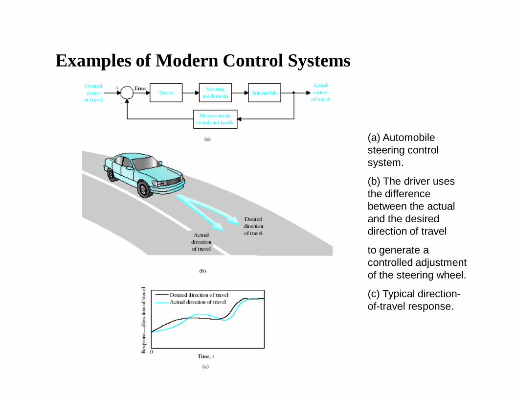
(a) Automobile steering control system.
(b) The driver uses the difference between the actual and the desired direction of travel
to generate a controlled adjustment of the steering wheel.
(c) Typical direction-of-travel response.
Examples of Modern Control Systems

Examples of Modern Control Systems

Control System Example
Advantages of Open Loop Control System
• Advantages
– Simple in construction and design– Economic– Easy maintenance– Not much problems with stability

Disadvantages of Open Loop Control System
• Disadvantages:– Inaccurate and unreliable because accuracy is
dependent on accuracy of calibration– Inaccurate results are obtained with parameter
variations, internal disturbances– To maintain the quality and accuracy, recalibration
of the system is necessary from time to time.

Advantages of Closed Loop Control System
• Advantages:– High accuracy– It senses change in output and corrects it– Reduced effect of non linearties– Facilitates automation
Disadvantages of Closed Loop Control System
• Disadvantages– Complicated in design– Costly maintenance– System may become unstable

Mathematical Modelling and Transfer Function
• We use quantitative mathematical models of physical systems to design and analyze control systems. The dynamic behavior is generally described by ordinary differential equations. We will consider a wide range of systems, including mechanical, hydraulic, and electrical.
• We will then proceed to obtain the input–output relationship for components and subsystems in the form of transfer functions. The transfer function blocks can be organized into block diagrams or signal-flow graphs to graphically depict the interconnections. Block diagrams (and signal-flow graphs) are very convenient and natural tools for designing and analyzing complicated control systems
Steps to approach Dynamic System Problems
• Define the system and its components• Formulate the mathematical model and list the
necessary assumptions• Write the differential equations describing the model• Solve the equations for the desired output variables• Examine the solutions and the assumptions• If necessary, reanalyze or redesign the system
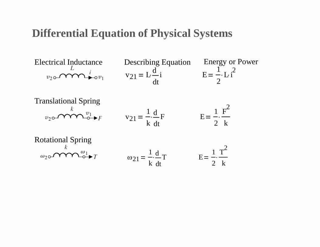
Differential Equation of Physical Systems
v21 Ltid
d E
12
L i2
v211k t
Fdd E
12
F2
k
211k t
Tdd E
12
T2
k
Electrical Inductance
Translational Spring
Rotational Spring
Describing Equation Energy or Power

Electrical Capacitance
Translational Mass
Rotational Mass
i Ctv21
dd E
12
M v212
F Mtv2
dd E
12
M v22
T Jt2
dd E
12
J 22
Differential Equation of Physical Systems
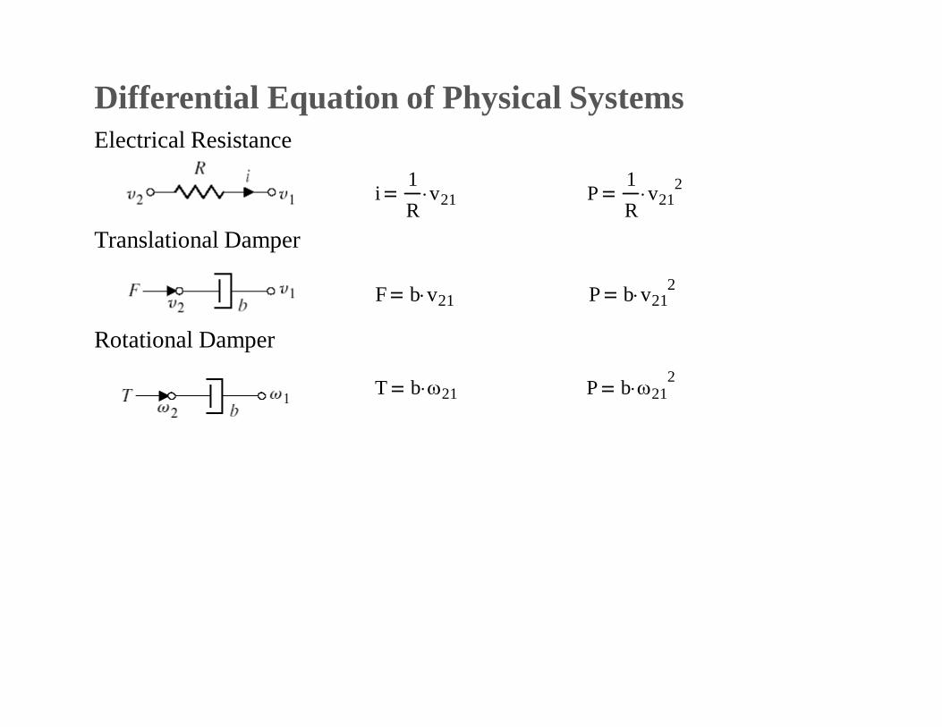
Electrical Resistance
Translational Damper
Rotational Damper
F b v21 P b v212
i1R
v21 P1R
v212
T b 21 P b 212
Differential Equation of Physical Systems

Differential Equation of Physical Systems
M 2ty t( )d
d
2 b
ty t( )d
d k y t( ) r t( )
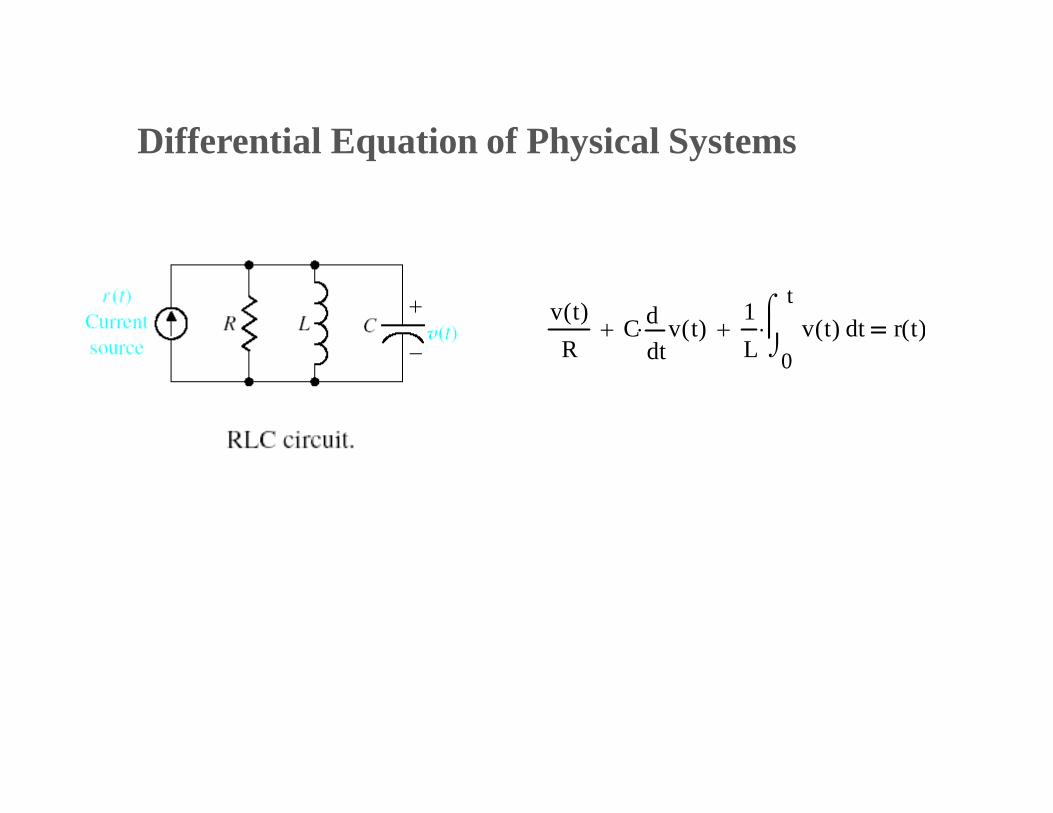
Differential Equation of Physical Systems
v t( )R
Ctv t( )d
d
1L 0
ttv t( )
d r t( )

Block Diagram Models
• Block diagrams are used as schematic representations of mathematical models
• The various pieces correspond to mathematical entities
• Can be rearranged to help simplify the equations used to model the system
• We will focus on one type of schematic diagram – feedback control systems

Processes
• Processes are represented by the blocks in block diagrams:
• Processes must have at least one input variable and at least one output variable
• Reclassify processes without input or output:
Input variable
Output variable
Processvariablevariable

Feedback Control Systems
• Many systems measure their output and use this measurement to control system behavior
• This is known as feedback control – the output is “fed back” into the system
• The summing junction is a special process that compares the input and the feedback
• Inputs to summing junction must have same units!
process
sensor
input output
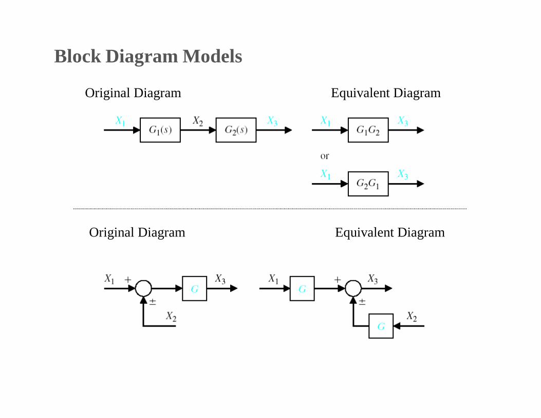
Block Diagram Models
Original Diagram Equivalent Diagram
Original Diagram Equivalent Diagram

Block Diagram Models
Original Diagram Equivalent Diagram
Original Diagram Equivalent Diagram

Block Diagram Models
Original Diagram Equivalent Diagram
Original Diagram Equivalent Diagram

Block Diagram Models
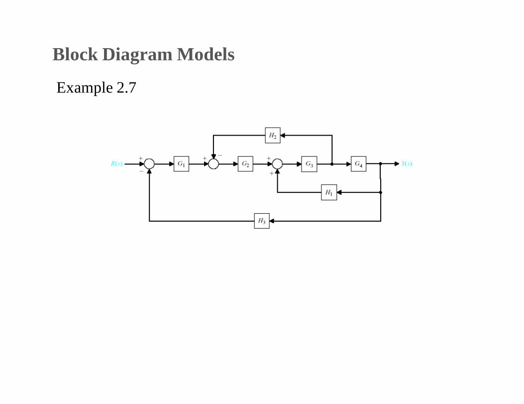
Block Diagram Models
Example 2.7

Block Diagram Models Example 2.7
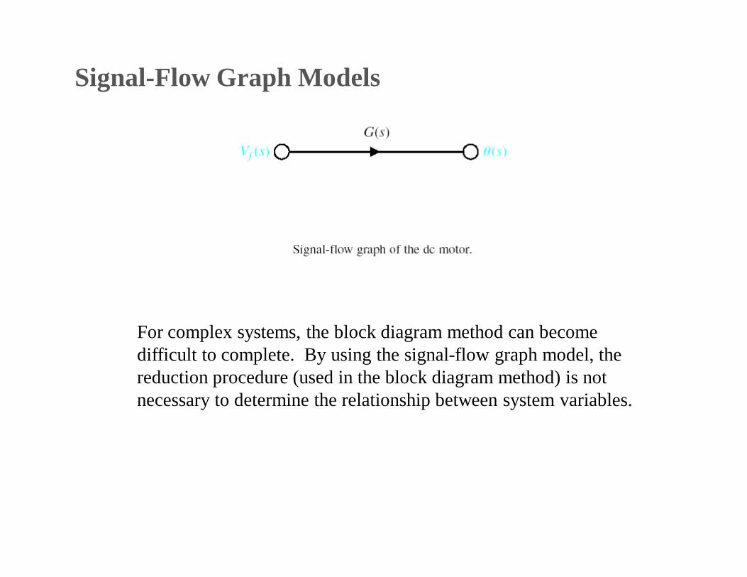
Signal-Flow Graph Models
For complex systems, the block diagram method can become difficult to complete. By using the signal-flow graph model, the reduction procedure (used in the block diagram method) is not necessary to determine the relationship between system variables.
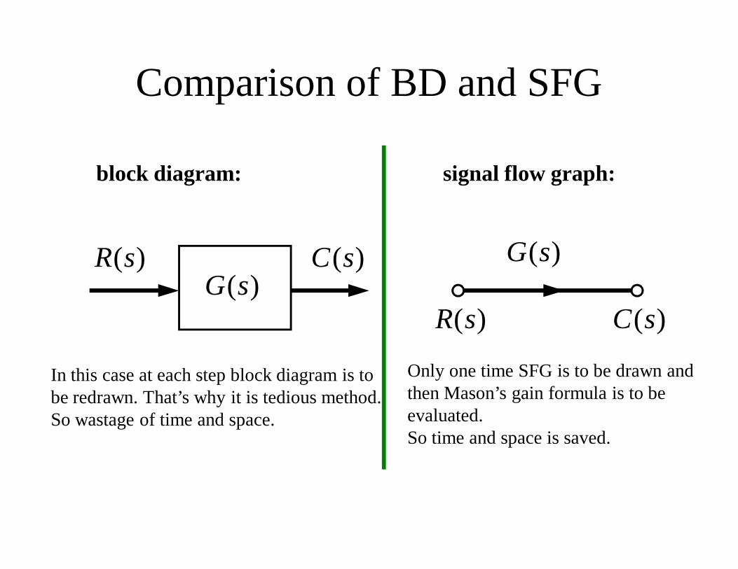
Comparison of BD and SFG
)(sR)(sG
)(sC )(sG
)(sR )(sC
block diagram: signal flow graph:
In this case at each step block diagram is to be redrawn. That’s why it is tedious method.So wastage of time and space.
Only one time SFG is to be drawn and then Mason’s gain formula is to be evaluated.So time and space is saved.

• A technique to reduce a signal-flow graph to a single transfer function requires the application of one formula.
• The transfer function, C(s)/R(s), of a system represented by asignal-flow graph is
k = number of forward pathPk = the kth forward path gain
∆ = 1 – (Σ loop gains) + (Σ non-touching loop gains taken two at a time) – (Σ non-touching loop gains taken three at a time)+ so on .
∆ k = 1 – (loop-gain which does not touch the forward path)
Mason’s Gain Formula

Ex: Signal-Flow Graph Models

P 1 =
P 2 =
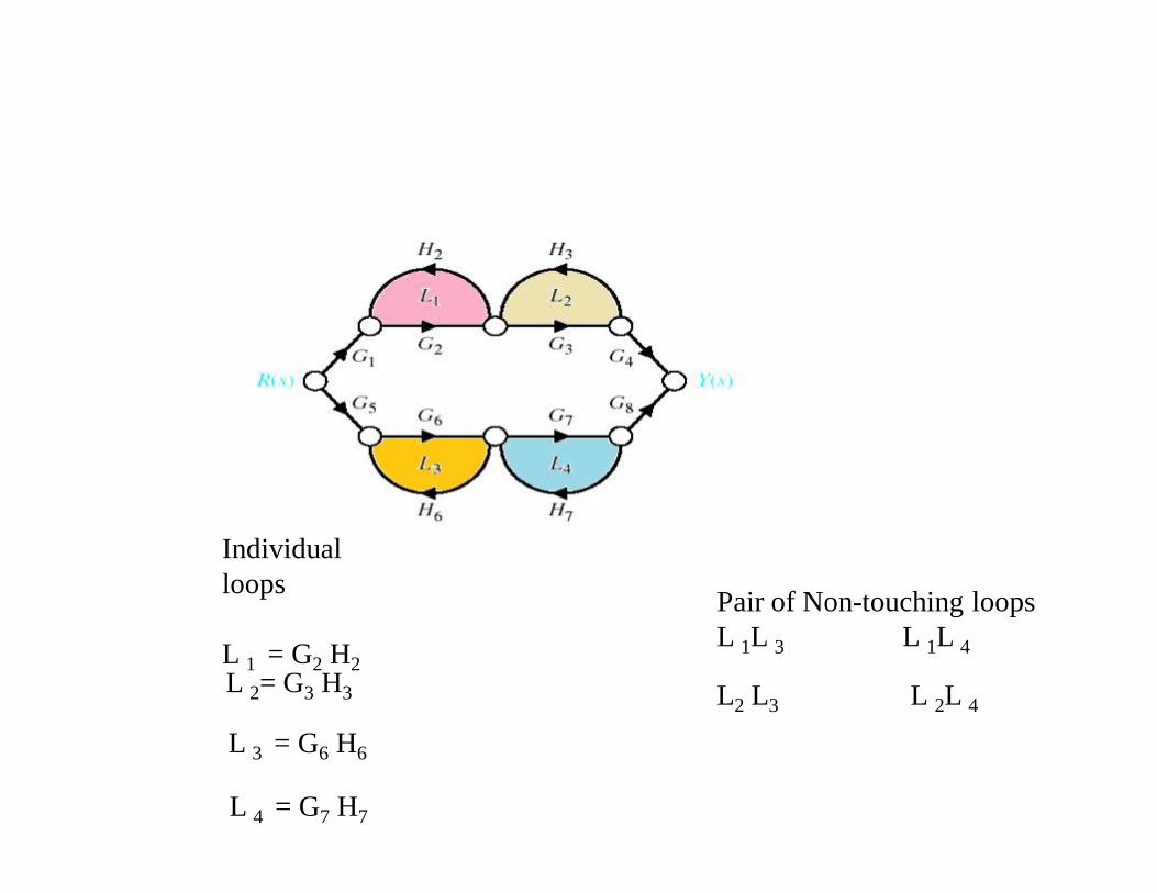
Individual loops
L 1 = G2 H2
L 4 = G7 H7
L 3 = G6 H6
L 2= G3 H3
Pair of Non-touching loops L 1L 3 L 1L 4
L2 L3 L 2L 4

..)21(1( LiLjLkiLjLLL
PRY kk
Ys( )Rs( )
G1 G2 G3 G4 1 L3 L4 G5 G6 G7 G8 1 L1 L2
1 L1 L2 L3 L4 L1 L3 L1 L4 L2 L3 L2 L4
UNIT - II
TIME RESPONSE ANALYSIS
Introduction• In time-domain analysis the response of a dynamic system to
an input is expressed as a function of time.
• It is possible to compute the time response of a system if thenature of input and the mathematical model of the system areknown.
• Usually, the input signals to control systems are not knownfully ahead of time.
• For example, in a radar tracking system, the position and thespeed of the target to be tracked may vary in a randomfashion.
• It is therefore difficult to express the actual input signalsmathematically by simple equations.
Standard Test Signals
• The characteristics of actual input signals are asudden shock, a sudden change, a constantvelocity, and constant acceleration.
• The dynamic behavior of a system is thereforejudged and compared under application ofstandard test signals – an impulse, a step, aconstant velocity, and constant acceleration.
• Another standard signal of great importance is asinusoidal signal.
Standard Test Signals
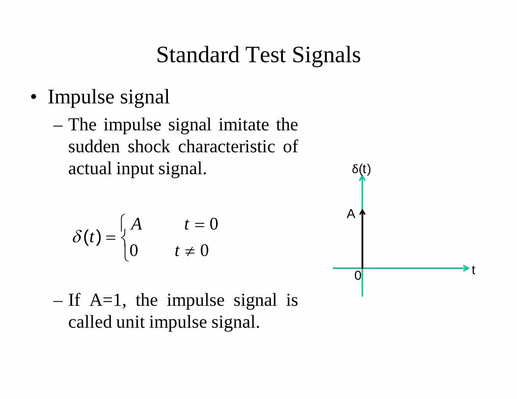
• Impulse signal– The impulse signal imitate the
sudden shock characteristic ofactual input signal.
– If A=1, the impulse signal iscalled unit impulse signal.
0 t
δ(t)
A
00
0t
tAt
)(
Standard Test Signals
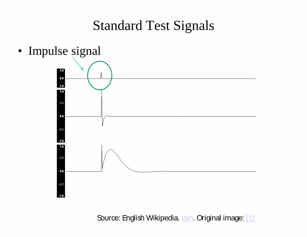
• Impulse signal
Source: English Wikipedia. Iain. Original image: [1]
Standard Test Signals
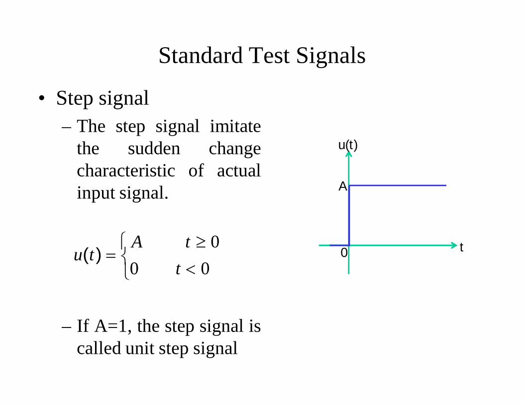
• Step signal– The step signal imitate
the sudden changecharacteristic of actualinput signal.
– If A=1, the step signal iscalled unit step signal
00
0t
tAtu
)( 0 t
u(t)
A

Standard Test Signals
• Ramp signal– The ramp signal imitate
the constant velocitycharacteristic of actualinput signal.
– If A=1, the ramp signalis called unit rampsignal
00
0t
tAttr
)(
0 t
r(t)
r(t)
unit ramp signal
r(t)
ramp signal with slope A

Standard Test Signals
• Parabolic signal– The parabolic signal
imitate the constantacceleration characteristicof actual input signal.
– If A=1, the parabolicsignal is called unitparabolic signal.
00
02
2
t
tAttp
)(
0 t
p(t)
parabolic signal with slope A
p(t)
Unit parabolic signal
p(t)

Relation between standard Test Signals
• Impulse
• Step
• Ramp
• Parabolic
00
0t
tAt
)(
00
0t
tAtu
)(
00
0t
tAttr
)(
00
02
2
t
tAttp
)(
dtd
dtd
dtd

Laplace Transform of Test Signals
• Impulse
• Step
00
0t
tAt
)(
AstL )()}({
00
0t
tAtu
)(
SAsUtuL )()}({
Laplace Transform of Test Signals
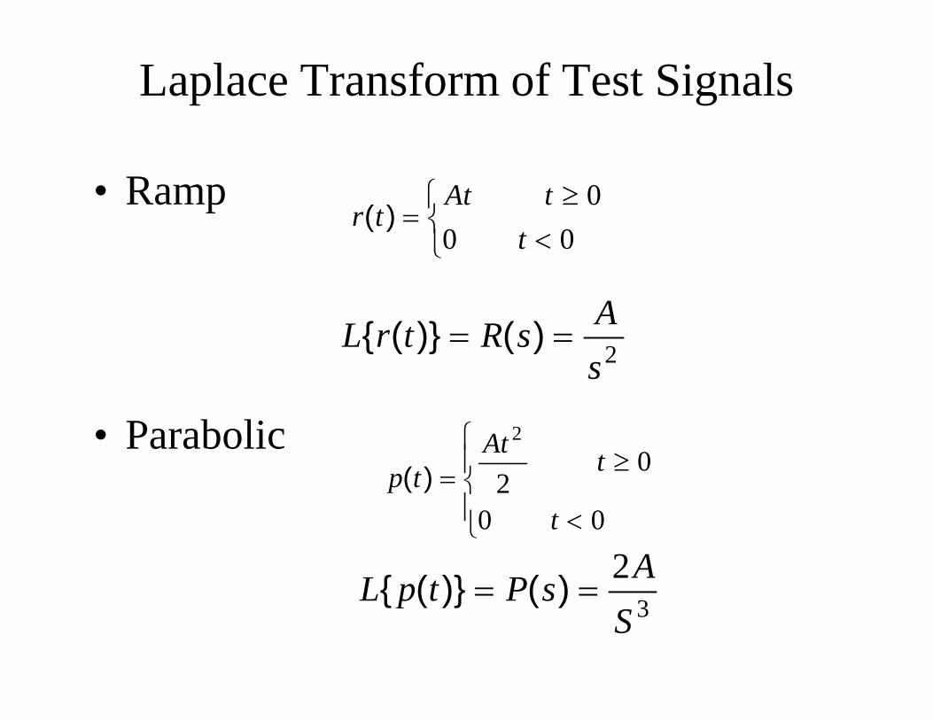
• Ramp
• Parabolic
2sAsRtrL )()}({
32S
AsPtpL )()}({
00
0t
tAttr
)(
00
02
2
t
tAttp
)(

Time Response of Control Systems
System
• The time response of any system has two components
• Transient response
• Steady-state response.
• Time response of a dynamic system response to an inputexpressed as a function of time.

Time Response of Control Systems
• When the response of the system is changed form rest orequilibrium it takes some time to settle down.
• Transient response is the response of a system from rest orequilibrium to steady state.
0 2 4 6 8 10 12 14 16 18 200
1
2
3
4
5
6x 10
Time (sec)
Response
Step Input
Transient Response
Stea
dy S
tate
Res
pons
e• The response of thesystem after the transientresponse is called steadystate response.

Time Response of Control Systems
• Transient response is dependent upon the system poles only andnot on the type of input.
• It is therefore sufficient to analyze the transient response using astep input.
• The steady-state response depends on system dynamics and theinput quantity.
• It is then examined using different test signals by final valuetheorem.

Introduction• We have already discussed the affect of location of poles and zeros
on the transient response of 1st order systems.
• Compared to the simplicity of a first-order system, a second-ordersystem exhibits a wide range of responses that must be analyzedand described.
• Varying a first-order system's parameter (T, K) simply changes thespeed and offset of the response
• Whereas, changes in the parameters of a second-order system canchange the form of the response.
• A second-order system can display characteristics much like a first-order system or, depending on component values, display dampedor pure oscillations for its transient response.
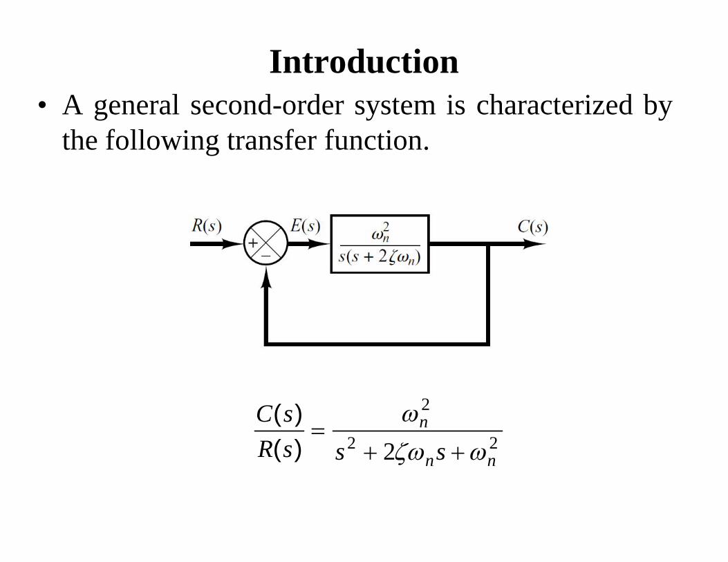
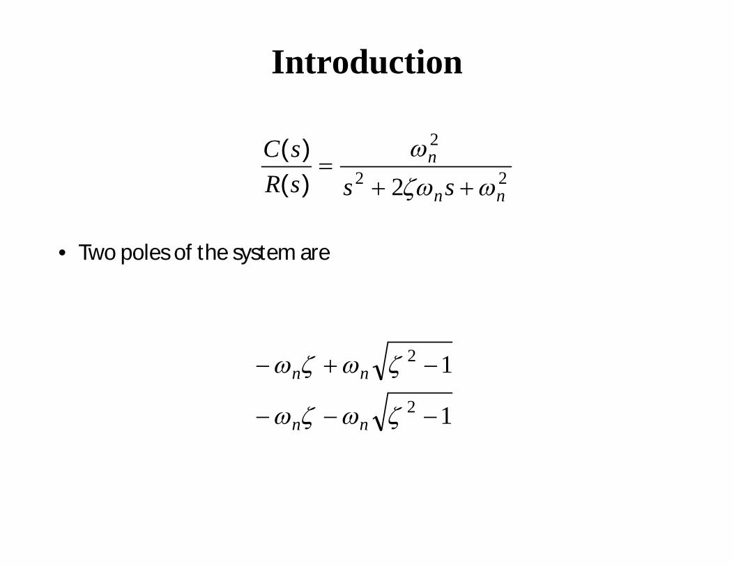
Introduction• A general second-order system is characterized by
the following transfer function.
22
2
2 nn
n
sssRsC
)()(
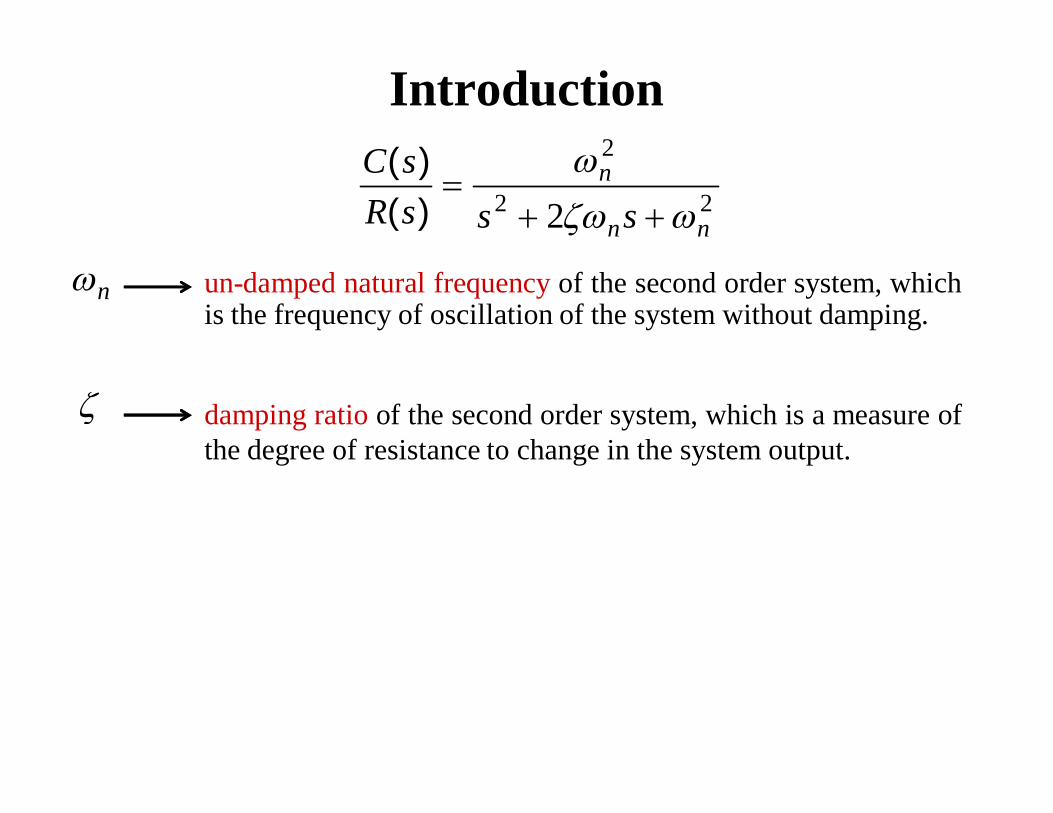
Introduction
un-damped natural frequency of the second order system, whichis the frequency of oscillation of the system without damping.
22
2
2 nn
n
sssRsC
)()(
n
damping ratio of the second order system, which is a measure ofthe degree of resistance to change in the system output.
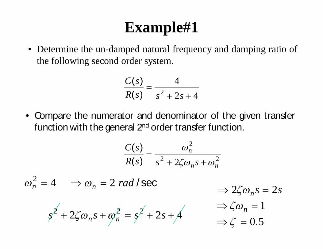
Example#1
424
2
sssRsC)()(
• Determine the un-damped natural frequency and damping ratio ofthe following second order system.
42 n
22
2
2 nn
n
sssRsC
)()(
• Compare the numerator and denominator of the given transferfunction with the general 2nd order transfer function.
sec/radn 2 ssn 22
422 222 ssss nn 50. 1 n
Introduction
22
2
2 nn
n
sssRsC
)()(
• Two poles of the system are
1
12
2
nn
nn
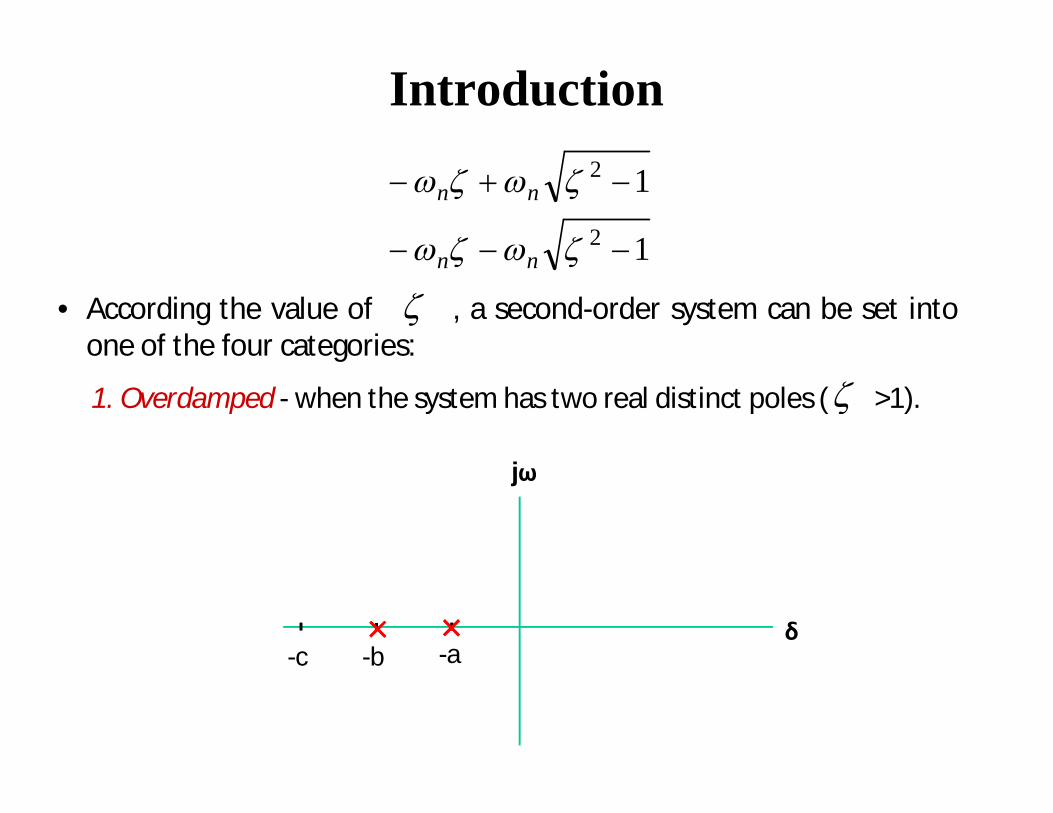
Introduction
• According the value of , a second-order system can be set intoone of the four categories:
1
12
2
nn
nn
1. Overdamped - when the system has two real distinct poles ( >1).
-a-b-cδ
jω
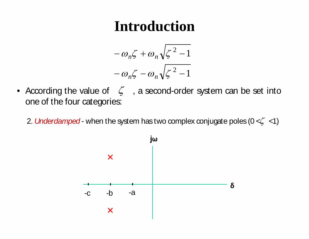
Introduction
• According the value of , a second-order system can be set intoone of the four categories:
1
12
2
nn
nn
2. Underdamped - when the system has two complex conjugate poles (0 < <1)
-a-b-cδ
jω

Introduction
• According the value of , a second-order system can be set intoone of the four categories:
1
12
2
nn
nn
3. Undamped - when the system has two imaginary poles ( = 0).
-a-b-cδ
jω

Introduction
• According the value of , a second-order system can be set intoone of the four categories:
1
12
2
nn
nn
4. Critically damped - when the system has two real but equal poles ( = 1).
-a-b-cδ
jω
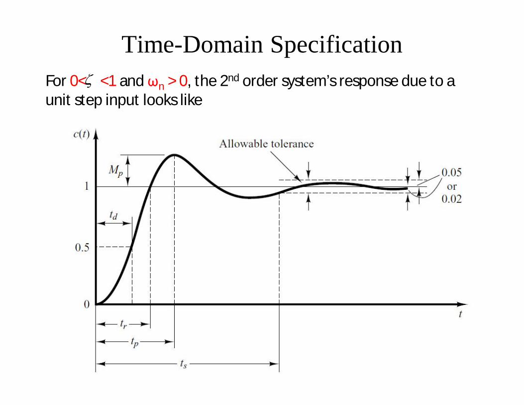
Time-Domain Specification
61
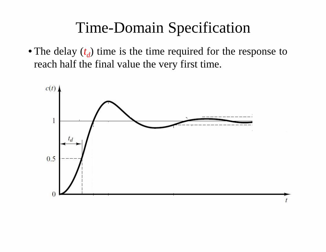
For 0< <1 and ωn > 0, the 2nd order system’s response due to a unit step input looks like
Time-Domain Specification
62
• The delay (td) time is the time required for the response toreach half the final value the very first time.
Time-Domain Specification
63
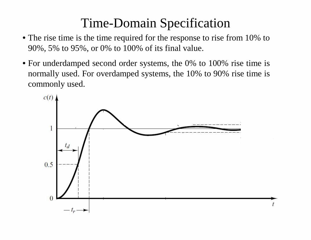
• The rise time is the time required for the response to rise from 10% to90%, 5% to 95%, or 0% to 100% of its final value.
• For underdamped second order systems, the 0% to 100% rise time isnormally used. For overdamped systems, the 10% to 90% rise time iscommonly used.

Time-Domain Specification
64
• The peak time is the time required for the response to reach the first peak of the overshoot.
6464

Time-Domain Specification
65
The maximum overshoot is the maximum peak value of theresponse curve measured from unity. If the final steady-statevalue of the response differs from unity, then it is common touse the maximum percent overshoot. It is defined by
The amount of the maximum (percent) overshoot directlyindicates the relative stability of the system.

Time-Domain Specification
66
• The settling time is the time required for the response curveto reach and stay within a range about the final value of sizespecified by absolute percentage of the final value (usually 2%or 5%).

S-Plane
δ
jω
• Natural Undamped Frequency.
n
• Distance from the origin of s-plane to pole is naturalundamped frequency inrad/sec.
S-Plane
δ
jω
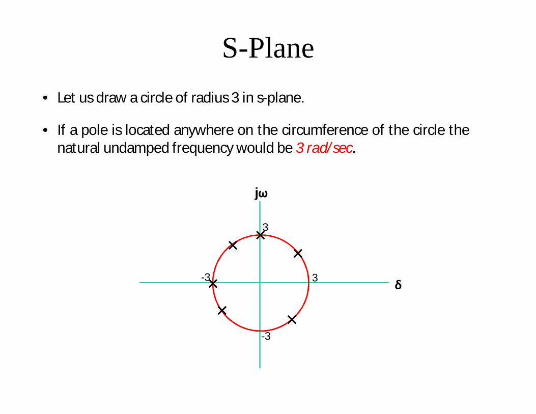
• Let us draw a circle of radius 3 in s-plane.
3
-3
-3
3
• If a pole is located anywhere on the circumference of the circle thenatural undamped frequency would be 3 rad/sec.
S-Plane
δ
jω
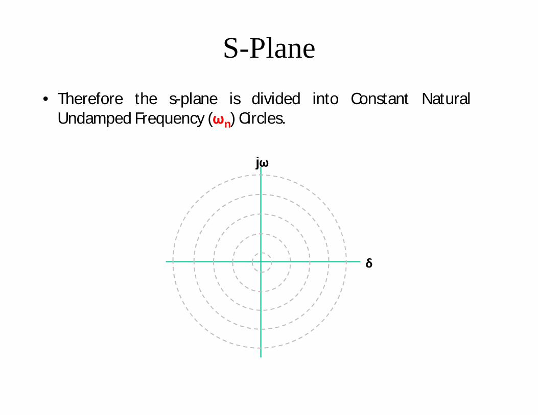
• Therefore the s-plane is divided into Constant NaturalUndamped Frequency (ωn) Circles.

S-Plane
δ
jω
• Damping ratio.
• Cosine of the angle betweenvector connecting origin andpole and –ve real axis yieldsdamping ratio.
cos

S-Plane
δ
jω
• For Underdamped system therefore, 900 10

S-Plane
δ
jω
• For Undamped system therefore,90 0

S-Plane
δ
jω
• For overdamped and critically damped systems therefore,
00
S-Plane
δ
jω
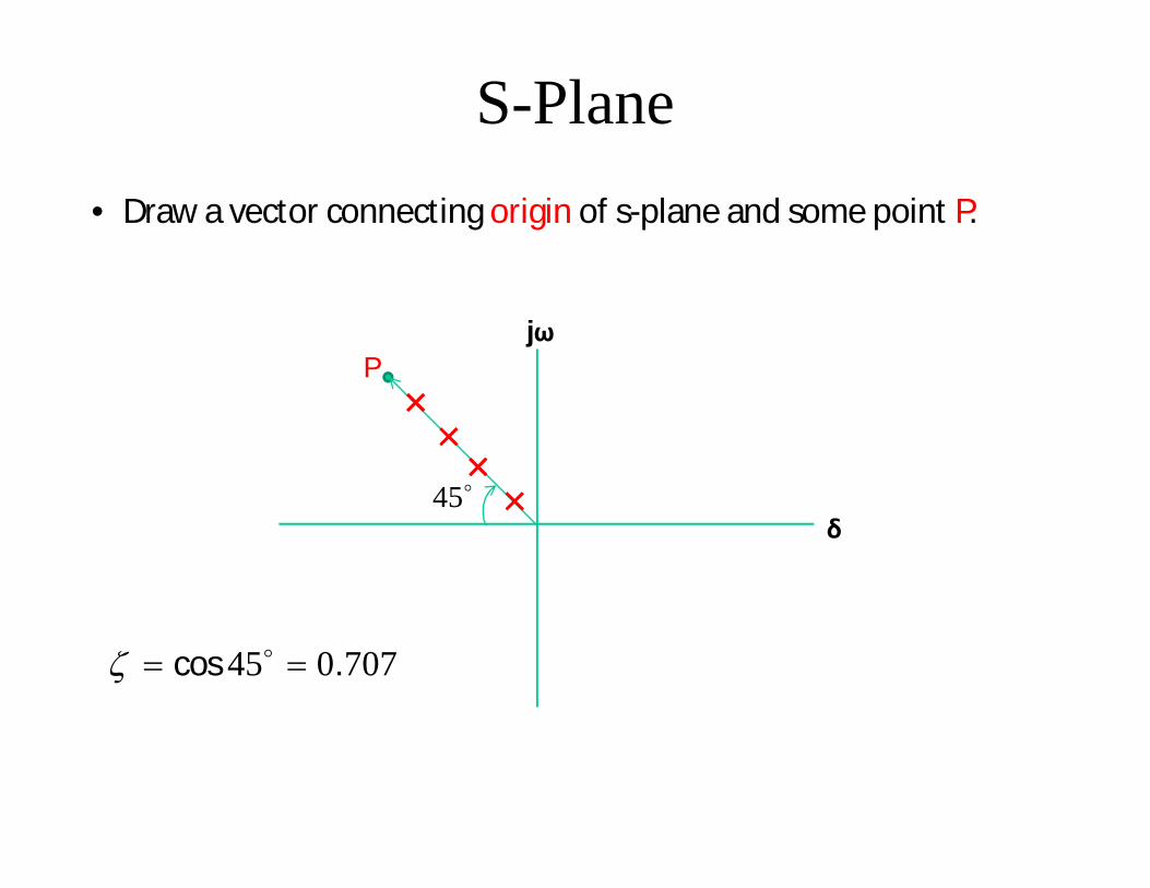
• Draw a vector connecting origin of s-plane and some point P.
P
45
707045 .cos

S-Plane
δ
jω
• Therefore, s-plane is divided into sections of constant damping ratio lines.
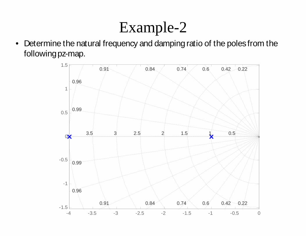
Example-2• Determine the natural frequency and damping ratio of the poles from the
following pz-map.
-4 -3.5 -3 -2.5 -2 -1.5 -1 -0.5 0-1.5
-1
-0.5
0
0.5
1
1.50.220.420.60.740.840.91
0.96
0.99
0.220.420.60.740.840.91
0.96
0.99
0.511.522.533.54

Example-3
• Determine the naturalfrequency and damping ratio ofthe poles from the given pz-map.
• Also determine the transferfunction of the system and statewhether system isunderdamped, overdamped,undamped or critically damped.
-3 -2.5 -2 -1.5 -1 -0.5 0-3
-2
-1
0
1
2
3
0.420.560.7
0.82
0.91
0.975
0.5
1
1.5
2
2.5
0.5
1
1.5
2
2.5
3
0.140.280.420.560.7
0.82
0.91
0.975
0.140.28
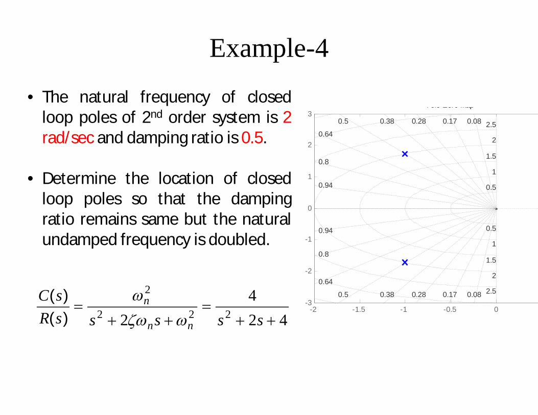
Example-4
• The natural frequency of closedloop poles of 2nd order system is 2rad/sec and damping ratio is 0.5.
• Determine the location of closedloop poles so that the dampingratio remains same but the naturalundamped frequency is doubled.
424
2 222
2
sssssRsC
nn
n
)()(
-2 -1.5 -1 -0.5 0-3
-2
-1
0
1
2
3
0.280.380.5
0.64
0.8
0.94
0.5
1
1.5
2
2.5
0.5
1
1.5
2
2.5
3
0.080.170.280.380.5
0.64
0.8
0.94
0.080.17
Pole-Zero Map
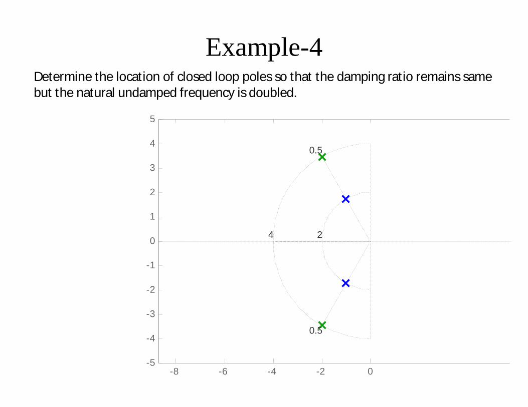
Example-4Determine the location of closed loop poles so that the damping ratio remains samebut the natural undamped frequency is doubled.
-8 -6 -4 -2 0-5
-4
-3
-2
-1
0
1
2
3
4
5
0.5
0.5
24
Pole-Zero Map

S-Plane
1
12
2
nn
nn
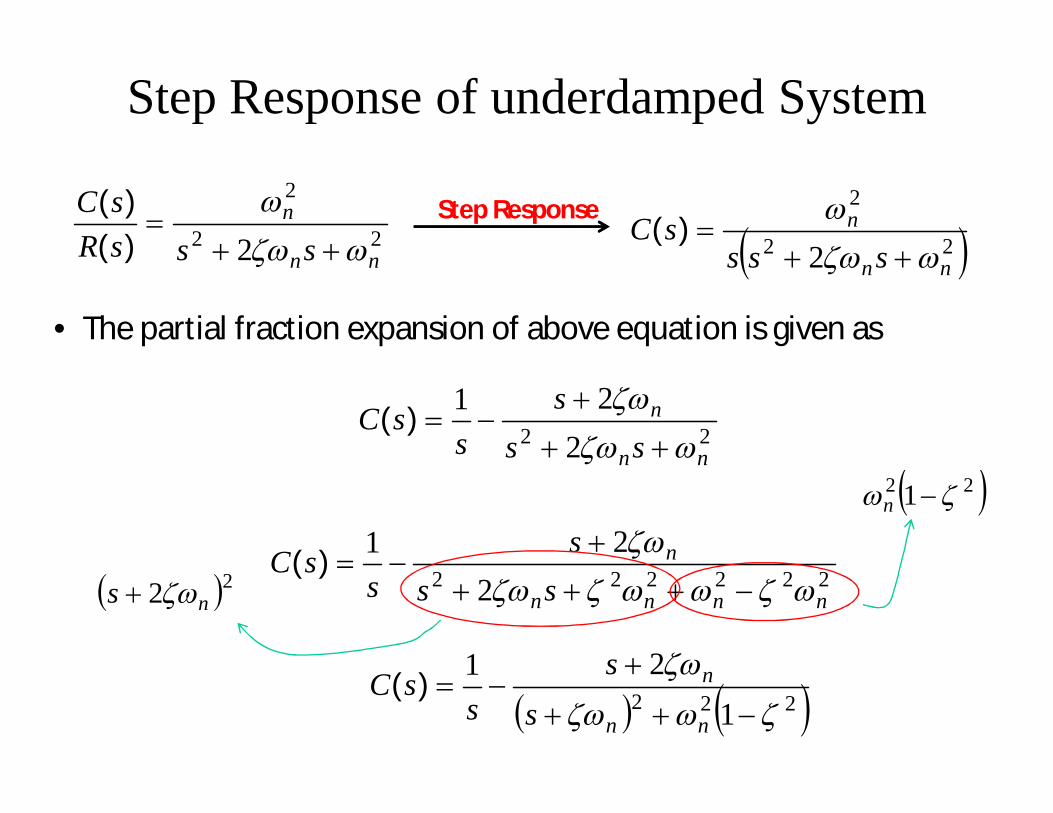
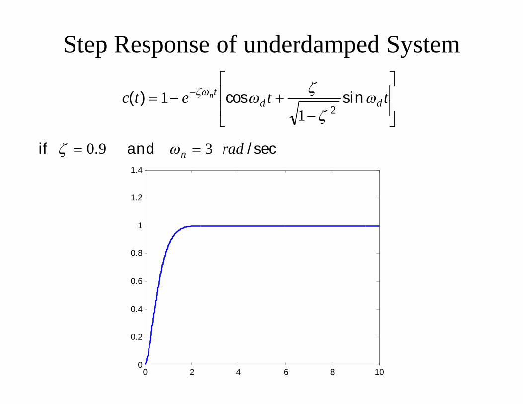
Step Response of underdamped System
222222 221
nnnn
n
sss
ssC
)(
• The partial fraction expansion of above equation is given as
22 221
nn
n
sss
ssC
)(
22 ns
22 1 n
222 121
nn
n
ss
ssC )(
22
2
2 nn
n
sssRsC
)()(
22
2
2 nn
n
ssssC
)(Step Response
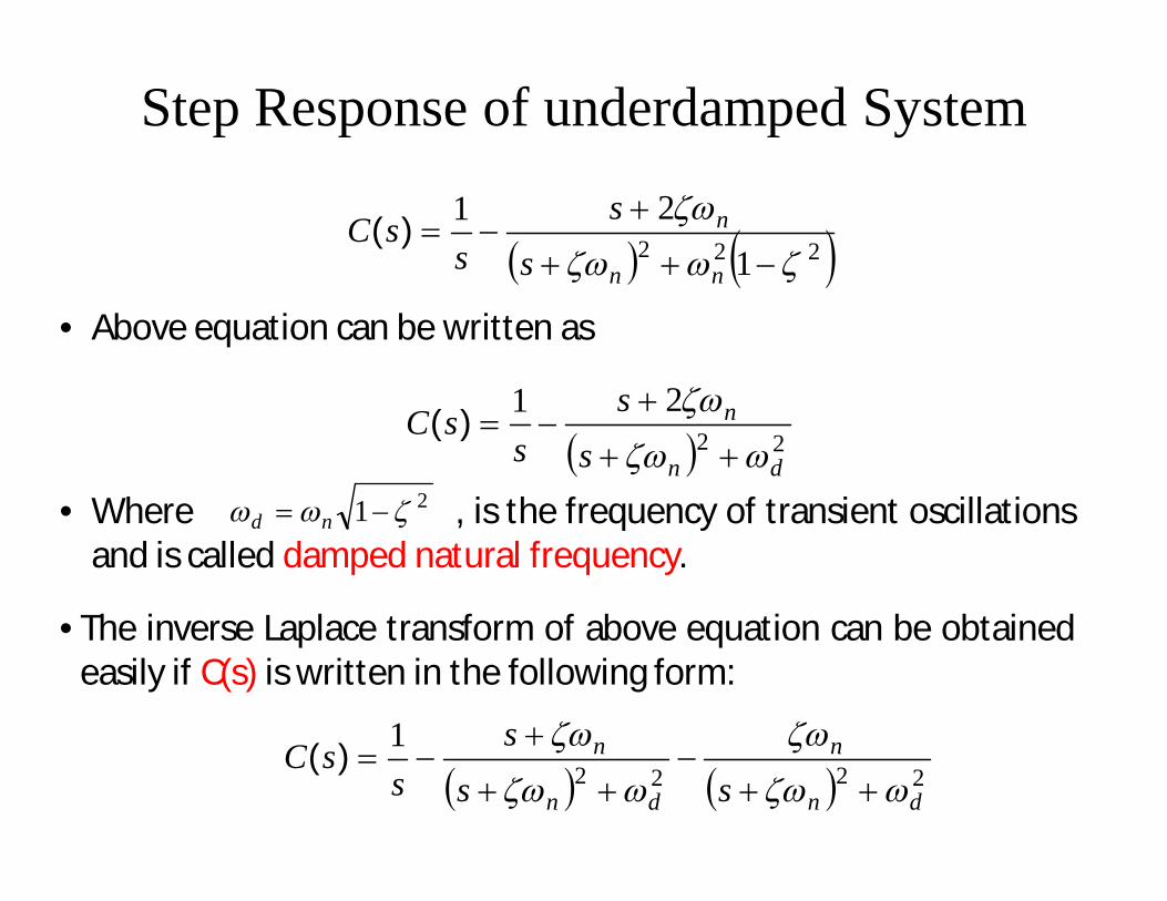
Step Response of underdamped System
• Above equation can be written as
222 121
nn
n
ss
ssC )(
2221
dn
n
ss
ssC
)(
21 nd• Where , is the frequency of transient oscillationsand is called damped natural frequency.
• The inverse Laplace transform of above equation can be obtainedeasily if C(s) is written in the following form:
22221
dn
n
dn
n
sss
ssC
)(
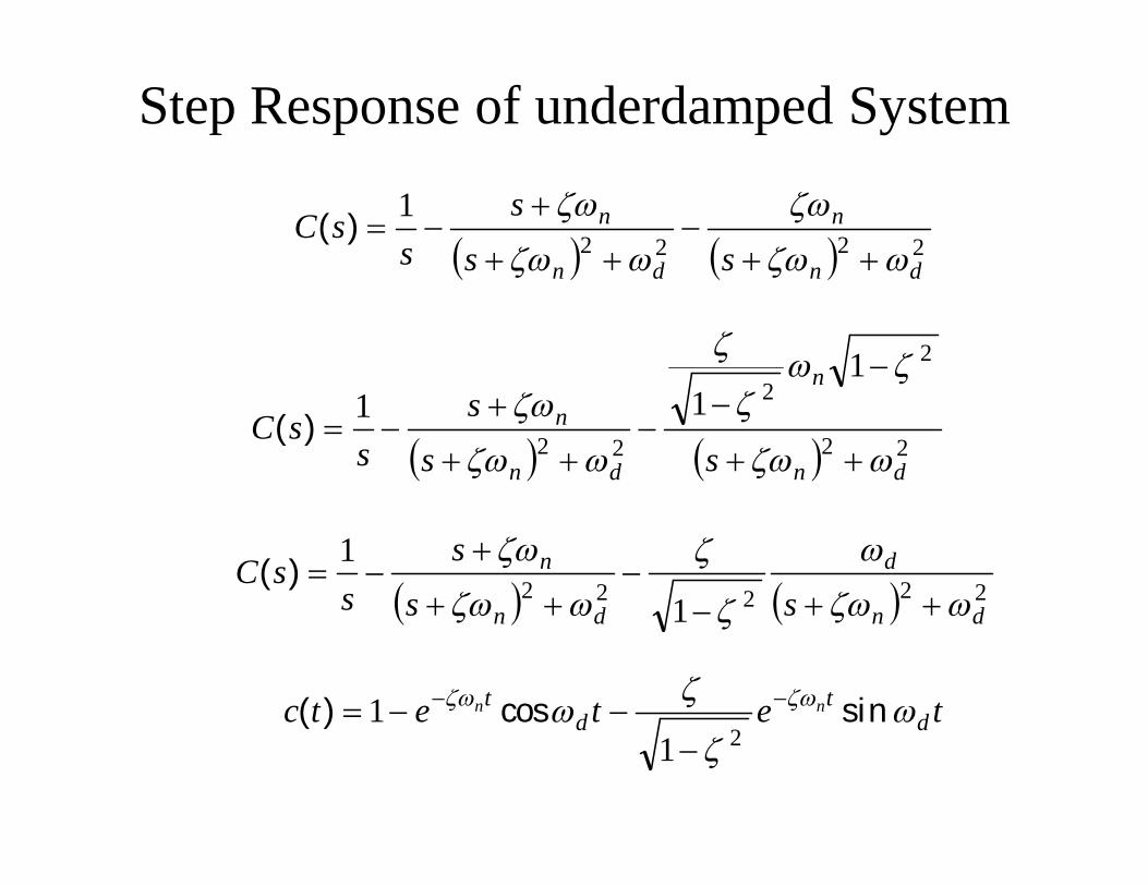
Step Response of underdamped System
22221
dn
n
dn
n
sss
ssC
)(
22
22
22
111
dn
n
dn
n
sss
ssC
)(
222221
1
dn
d
dn
n
sss
ssC
)(
tetetc dt
dt nn
sincos)(
211

Step Response of underdamped System
tetetc dt
dt nn
sincos)(
211
ttetc dd
tn
sincos)(21
1
n
nd
21• When 0
ttc ncos)( 1
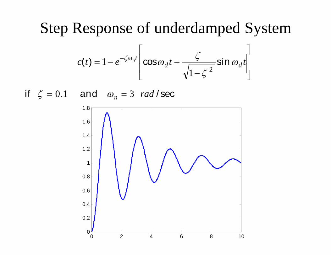
Step Response of underdamped System
ttetc dd
tn
sincos)(
211
sec/. radn and if 310
0 2 4 6 8 100
0.2
0.4
0.6
0.8
1
1.2
1.4
1.6
1.8

Step Response of underdamped System
ttetc dd
tn
sincos)(
211
sec/. radn and if 350
0 2 4 6 8 100
0.2
0.4
0.6
0.8
1
1.2
1.4
Step Response of underdamped System
ttetc dd
tn
sincos)(
211
sec/. radn and if 390
0 2 4 6 8 100
0.2
0.4
0.6
0.8
1
1.2
1.4
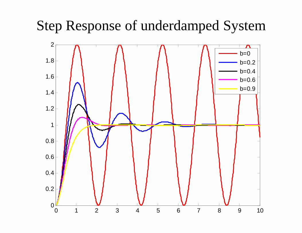
Step Response of underdamped System
0 1 2 3 4 5 6 7 8 9 100
0.2
0.4
0.6
0.8
1
1.2
1.4
1.6
1.8
2
b=0b=0.2b=0.4b=0.6b=0.9

Step Response of underdamped System
0 1 2 3 4 5 6 7 8 9 100
0.2
0.4
0.6
0.8
1
1.2
1.4
wn=0.5wn=1wn=1.5wn=2wn=2.5

Time Domain Specifications of Underdamped system

Time Domain Specifications (Rise Time)
ttetc dd
tn
sincos)(
211
equation above in Put rtt
rdrdt
r ttetc rn
sincos)(
211
1)c(tr Where
rdrdt tte rn
sincos21
0
0 rnte
rdrd tt
sincos21
0

Time Domain Specifications (Rise Time)
as writen-re be can equation above
01 2
rdrd tt
sincos
rdrd tt
cossin21
21
rd ttan
2
1 1tanrd t

Time Domain Specifications (Rise Time)
2
1 1tanrd t
n
n
drt
21 11 tan
drt
ba1 tan
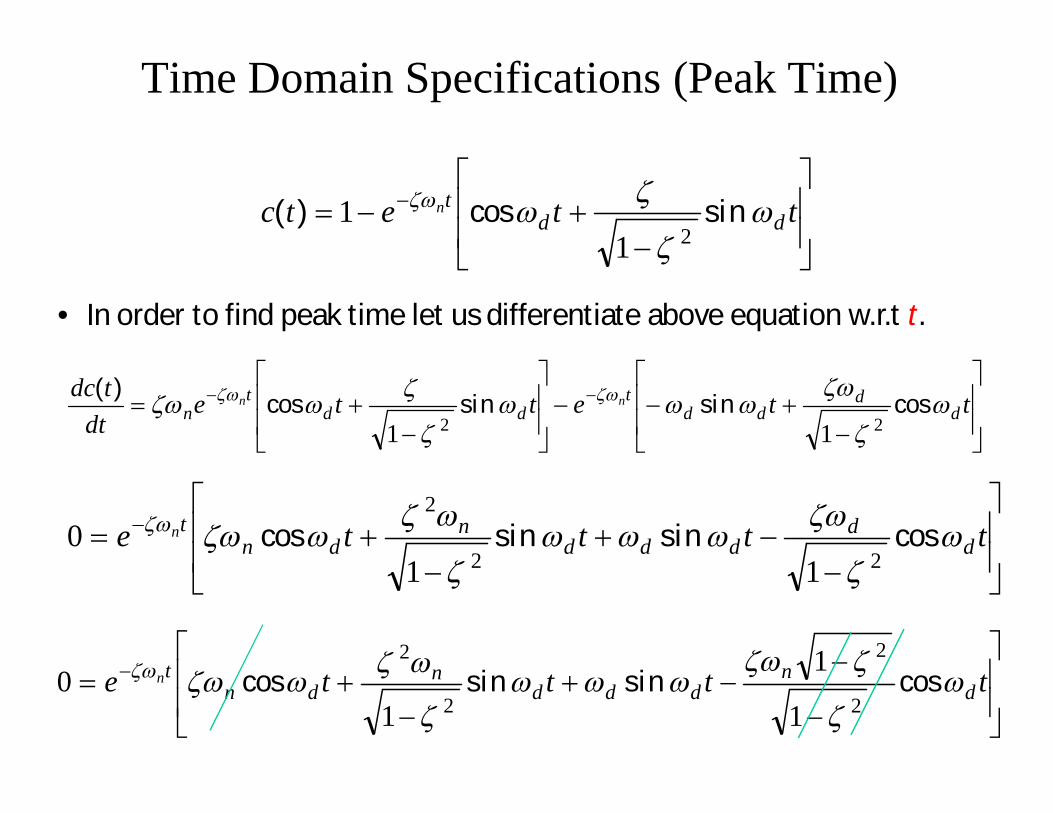
Time Domain Specifications (Peak Time)
ttetc dd
tn
sincos)(
211
• In order to find peak time let us differentiate above equation w.r.t t.
ttette
dttdc
dd
ddt
ddt
nnn
cossinsincos)(
22 11
tttte d
dddd
ndn
tn
cossinsincos
22
2
110
tttte d
nddd
ndn
tn
cossinsincos
2
2
2
2
1
1
10

Time Domain Specifications (Peak Time)
tttte d
nddd
ndn
tn
cossinsincos
2
2
2
2
1
1
10
01 2
2
tte dddntn
sinsin
0 tne 01 2
2
tt ddd
n
sinsin
01 2
2
d
nd t
sin

Time Domain Specifications (Peak Time)
01 2
2
d
nd t
sin
01 2
2
d
n
0tdsin
01 sintd
dt
,,, 20
• Since for underdamped stable systems first peak is maximum peaktherefore,
dpt
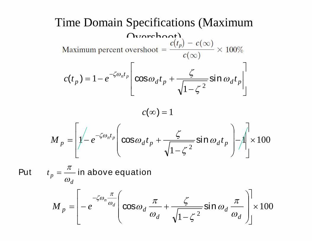
Time Domain Specifications (Maximum Overshoot)
pdpdt
p ttetc pn
sincos)(
211
1)(c
10011
12
pdpdt
p tteM pn
sincos
equation above in Putd
pt
1001 2
dd
ddp
dn
eM
sincos
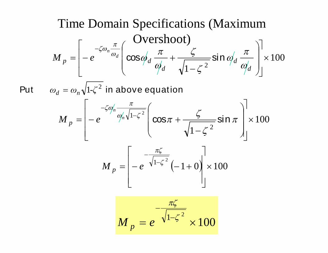
Time Domain Specifications (Maximum Overshoot)
1001 2
dd
ddp
dn
eM
sincos
1001 2
1 2
sincosnn
eM p
1000121
eM p
10021
eM p
equation above in Put 21-ζωω nd

Time Domain Specifications (Settling Time)
ttetc dd
tn
sincos)(
211
12 nn
nT
1
Real Part Imaginary Part

Time Domain Specifications (Settling Time)
nT
1
• Settling time (2%) criterion• Time consumed in exponential decay up to 98% of the input.
ns Tt
44
• Settling time (5%) criterion• Time consumed in exponential decay up to 95% of the input.
ns Tt
33
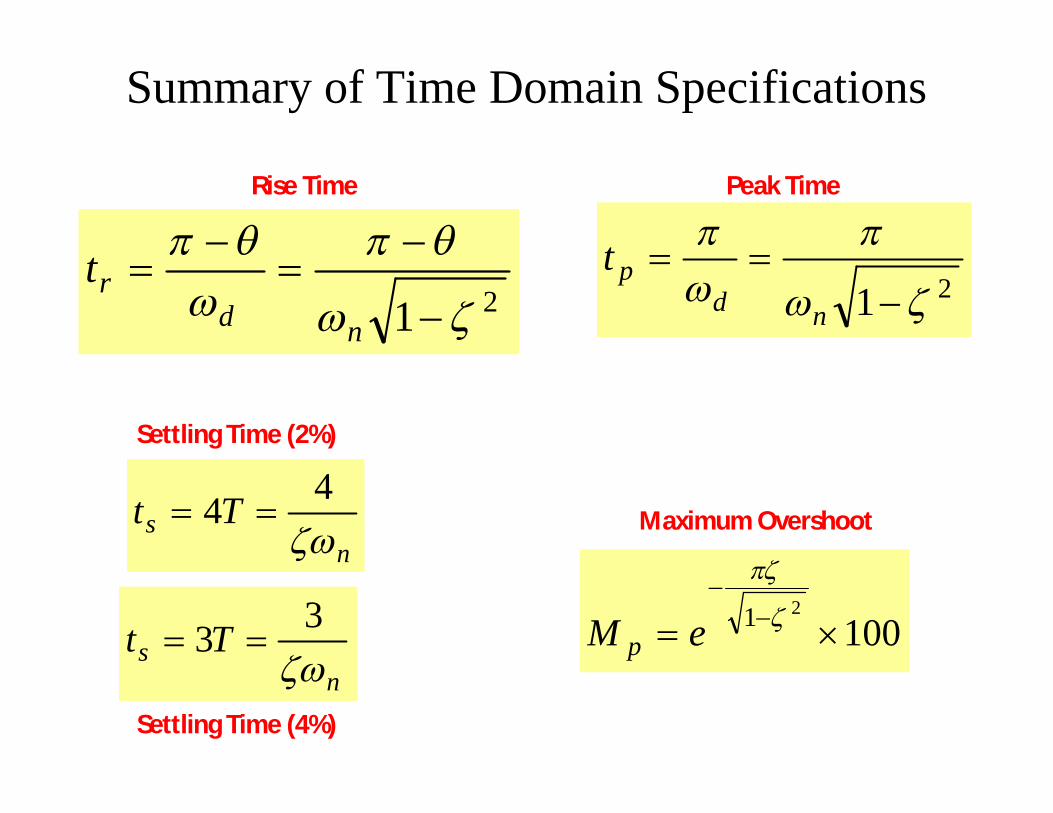
Summary of Time Domain Specifications
ns Tt
44
ns Tt
33 100
21
eM p
21
ndpt
21
ndrt
Rise Time Peak Time
Settling Time (2%)
Settling Time (4%)
Maximum Overshoot

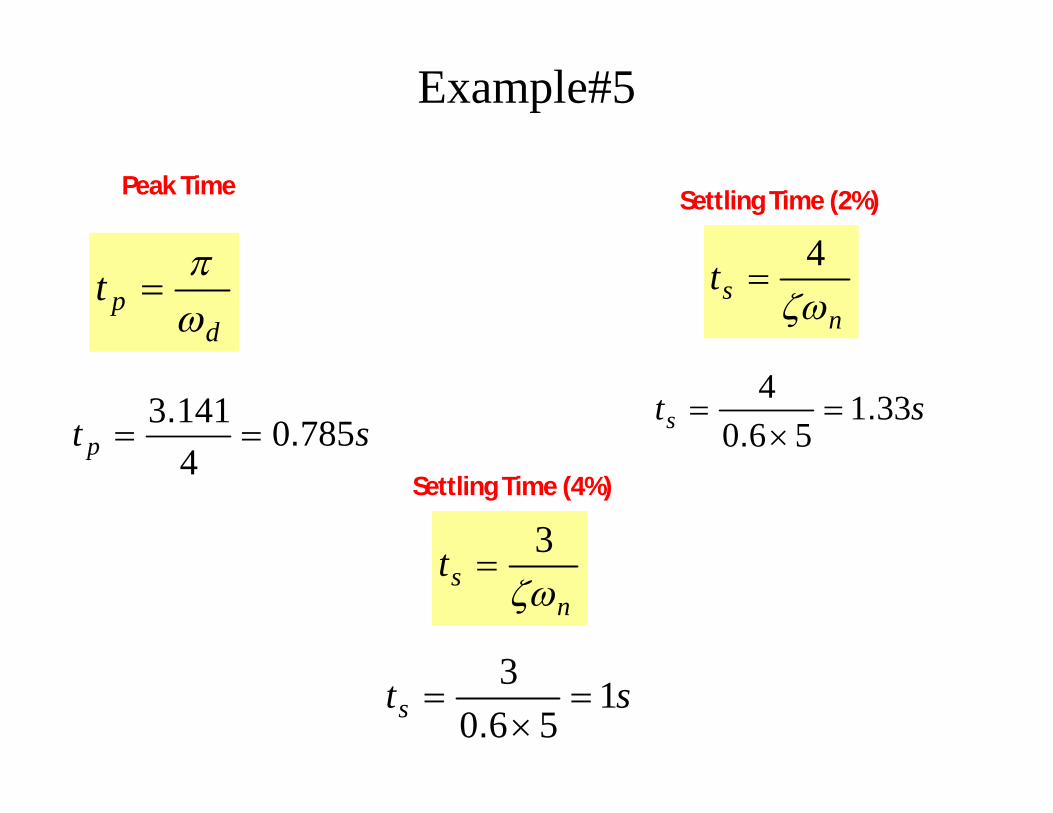
Example#5• Consider the system shown in following figure, where
damping ratio is 0.6 and natural undamped frequency is 5rad/sec. Obtain the rise time tr, peak time tp, maximumovershoot Mp, and settling time 2% and 5% criterion ts whenthe system is subjected to a unit-step input.
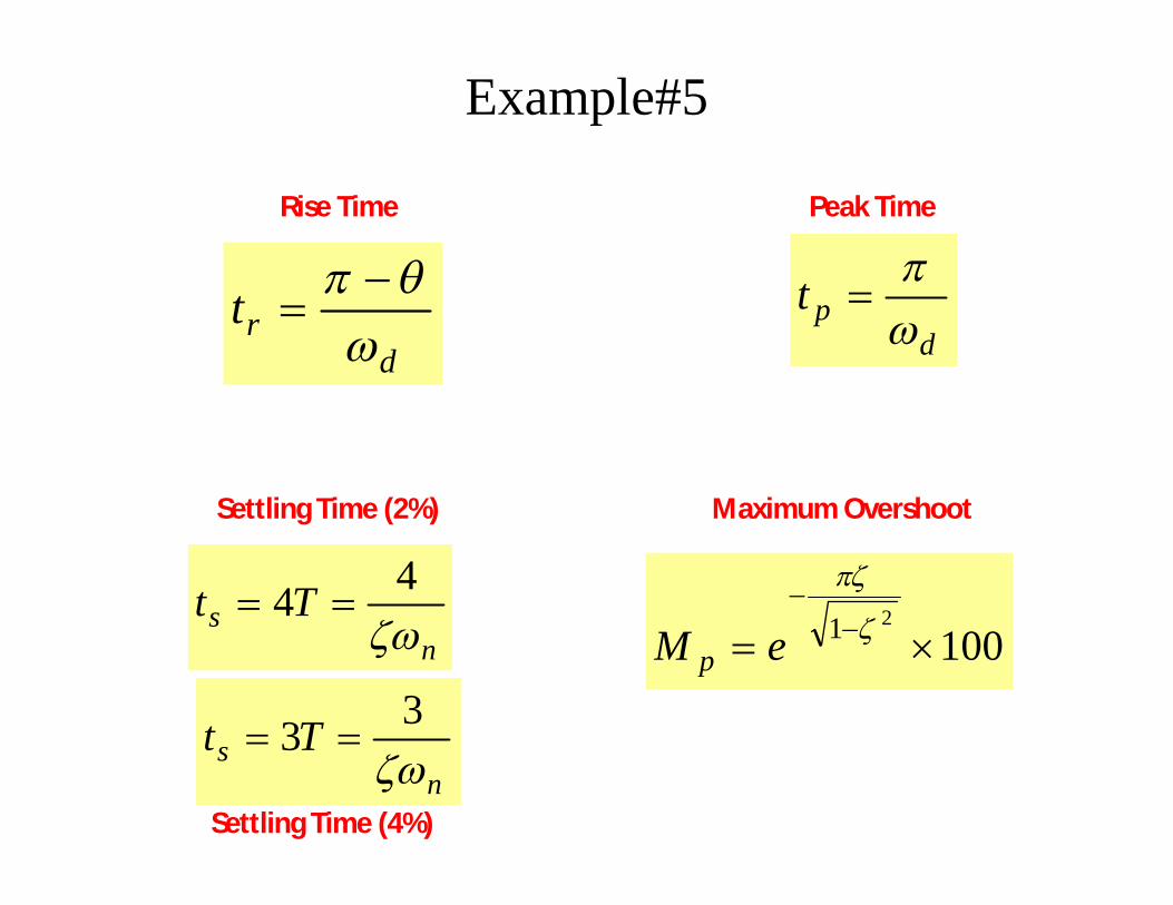
Example#5
ns Tt
44
10021
eM p
dpt
d
rt
Rise Time Peak Time
Settling Time (2%) Maximum Overshoot
ns Tt
33
Settling Time (4%)
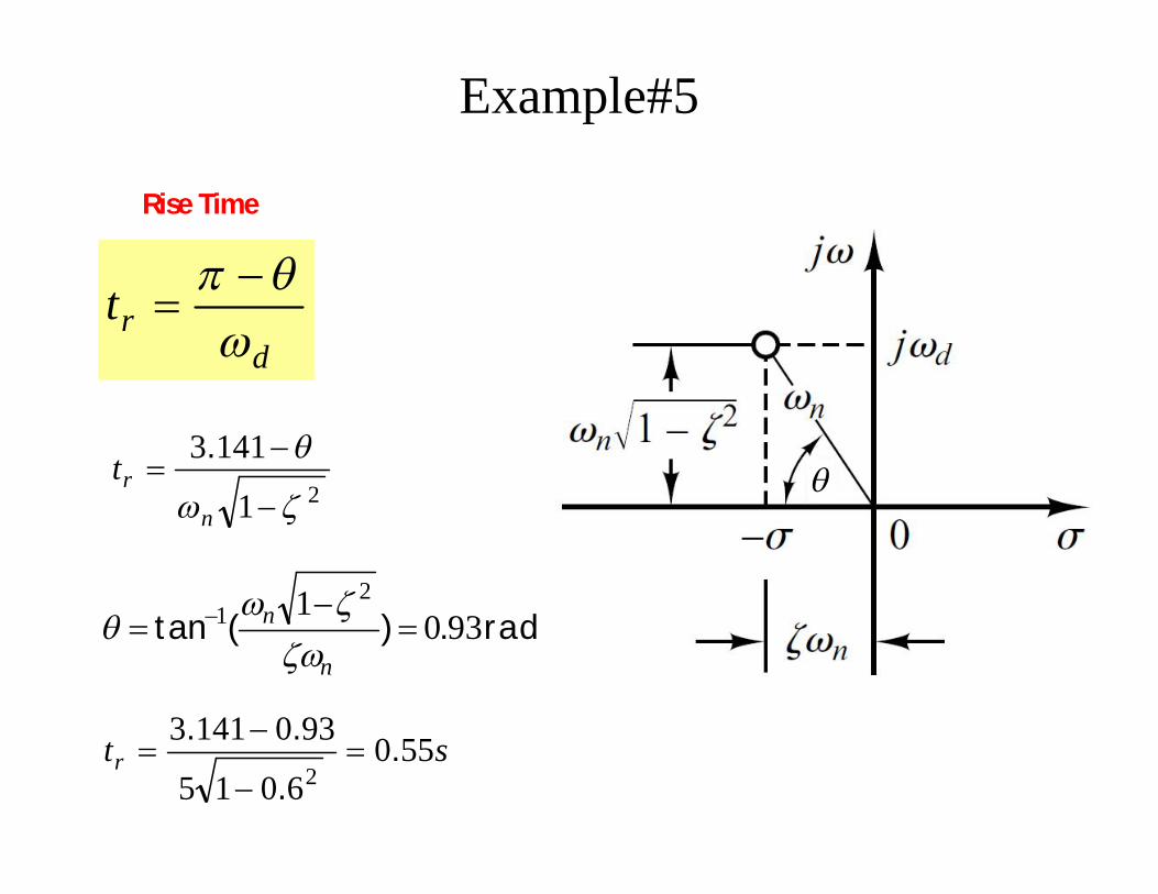
Example#5
drt
Rise Time
21
1413
nrt
.
rad 9301 2
1 .)(tan
n
n
str 5506015
93014132
....
Example#5
nst
4
dpt
Peak Time Settling Time (2%)
nst
3
Settling Time (4%)
st p 785041413 ..
sts 331
5604 .
.
sts 1560
3
.

Example#5
10021
eM p
Maximum Overshoot
1002601
601413
...
eM p
1000950 .pM
%.59pM

Example#5Step Response
Time (sec)
Ampl
itude
0 0.2 0.4 0.6 0.8 1 1.2 1.4 1.60
0.2
0.4
0.6
0.8
1
1.2
1.4
Mp
Rise Time

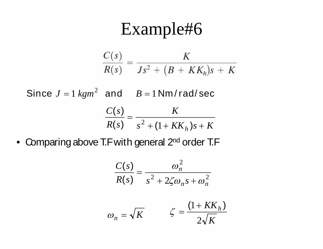
Example#6• For the system shown in Figure-(a), determine the values of gain K
and velocity-feedback constant Kh so that the maximum overshootin the unit-step response is 0.2 and the peak time is 1 sec. Withthese values of K and Kh, obtain the rise time and settling time.Assume that J=1 kg-m2 and B=1 N-m/rad/sec.

Example#6
Example#6
Nm/rad/sec and Since 11 2 BkgmJ
KsKKsK
sRsC
h
)()()(
12
22
2
2 nn
n
sssRsC
)()(
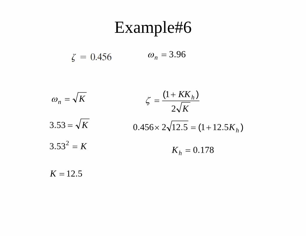
• Comparing above T.F with general 2nd order T.F
Kn KKKh
21 )(

Example#6
• Maximum overshoot is 0.2.
Kn KKKh
21 )(
2021 .ln)ln(
e
• The peak time is 1 sec
dpt
245601
1413
..
n
21
14131
n
.
533.n
Example#6
Kn K
KKh
21 )(
963.n
K533.
512
533 2
.
.
K
K
).(.. hK512151224560
1780.hK
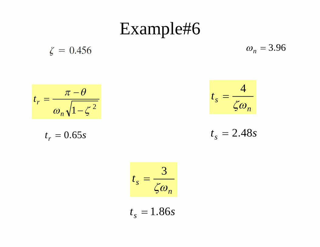
Example#6963.n
nst
4
nst
3
21
nrt
str 650. sts 482.
sts 861.
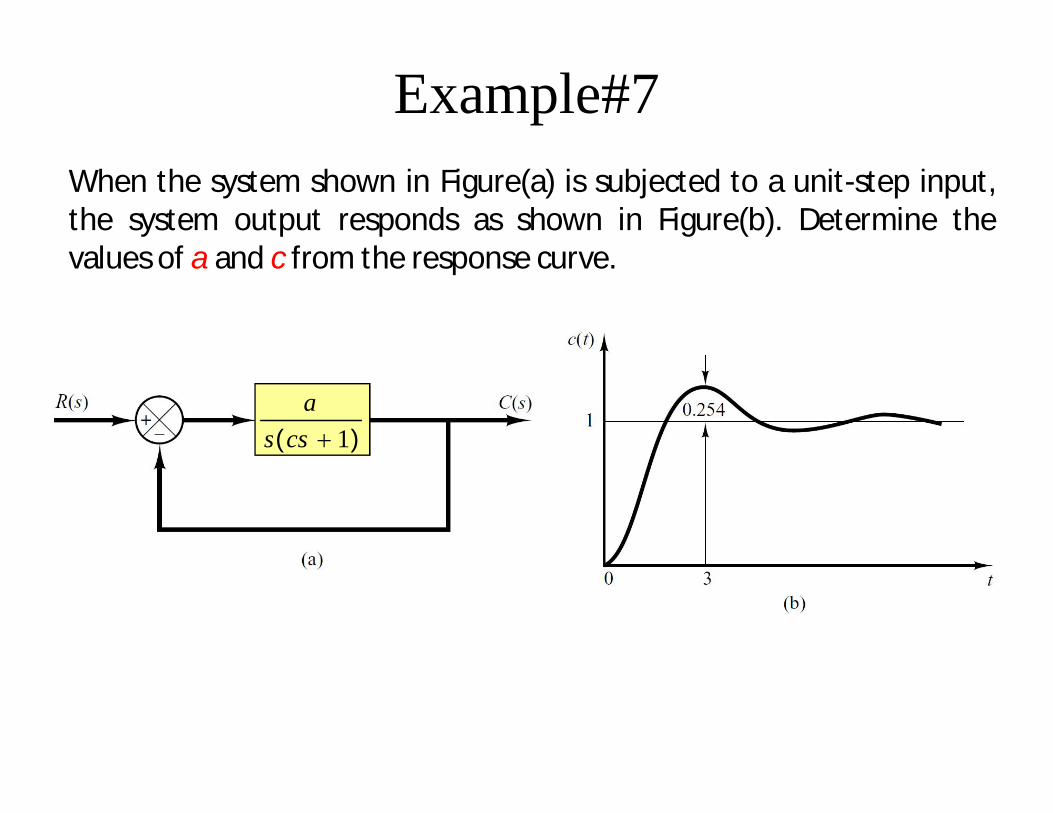
Example#7When the system shown in Figure(a) is subjected to a unit-step input,the system output responds as shown in Figure(b). Determine thevalues of a and c from the response curve.
)( 1cssa

Example#8Figure (a) shows a mechanical vibratory system. When 2 lb of force(step input) is applied to the system, the mass oscillates, as shown inFigure (b). Determine m, b, and k of the system from this responsecurve.
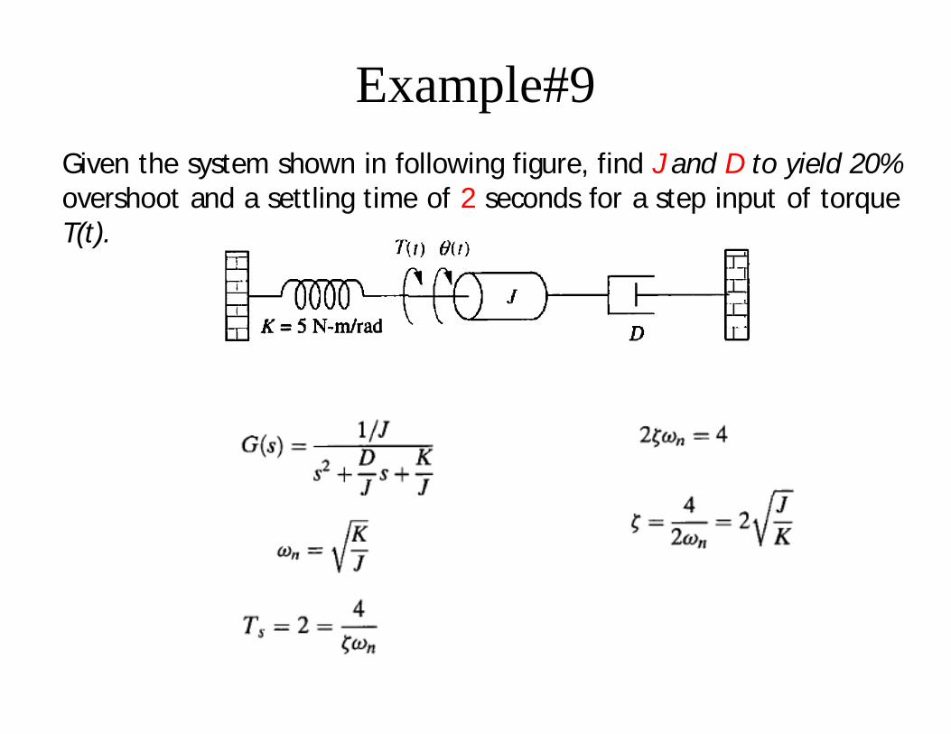
Example#9Given the system shown in following figure, find J and D to yield 20%overshoot and a settling time of 2 seconds for a step input of torqueT(t).

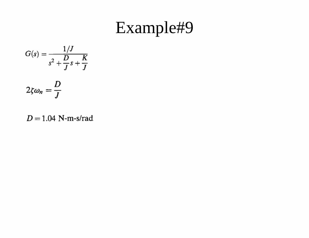
Example#9
Example#9

Step Response of critically damped System ( )
• The partial fraction expansion of above equation is given as
22
n
n
ssRsC
)()(
22
n
n
sssC
)(Step Response
22
2
nnn
n
sC
sB
sA
ss
211
n
n
n ssssC
)(
teetc tn
t nn 1)(
tetc ntn 11)(
1
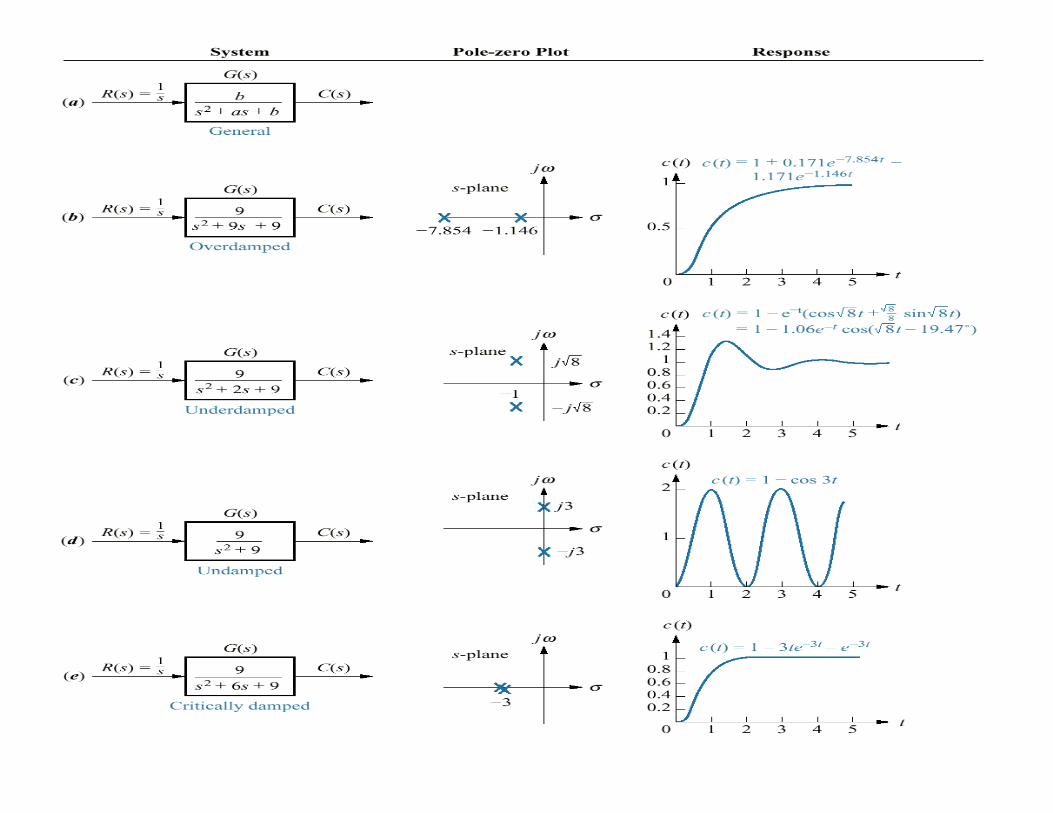
Step Response of overdamped and undamped Systems
• Home Work
121
122
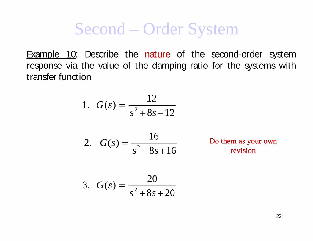
Example 10: Describe the nature of the second-order systemresponse via the value of the damping ratio for the systems withtransfer function
Second – Order System
12812)(.1 2
ss
sG
16816)(.2 2
ss
sG
20820)(.3 2
ss
sG
Do them as your own Do them as your own revisionrevision

STABILITY IN TIME DOMAIN
UNIT - III
The Concept of Stability
A stable system is a dynamic system with a bounded response to a bounded input.
Absolute stability is a stable/not stable characterization for a closed-loop feedback system. Given that a system is stable we can further characterize the degree of stability, or the relative stability.
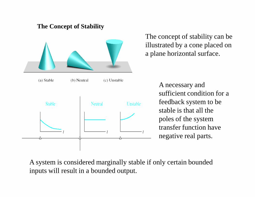
The Concept of StabilityThe concept of stability can be illustrated by a cone placed on a plane horizontal surface.
A necessary and sufficient condition for a feedback system to be stable is that all the poles of the system transfer function have negative real parts.
A system is considered marginally stable if only certain bounded inputs will result in a bounded output.
The Routh-Hurwitz Stability Criterion
It was discovered that all coefficients of the characteristic polynomial must have the same sign and non-zero if all the roots are in the left-hand plane.
These requirements are necessary but not sufficient. If the above requirements are not met, it is known that the system is unstable. But, if the requirements are met, we still must investigate the system further to determine the stability of the system.
The Routh-Hurwitz criterion is a necessary and sufficient criterion for the stability of linear systems.
The Routh-Hurwitz Stability Criterion
31
31
11
31
42
13
31
2
11
3211
10
5313
5312
5311
42
012
21
1
1
1
1
0
nn
nn
nn
nn
nn
nn
nn
nn
nn
nnnnn
n
nnnn
nnnn
nnnn
nnnn
nn
nn
nn
bbaa
bc
aaaa
ab
aaaa
aaaaaab
hs
cccsbbbsaaasaaas
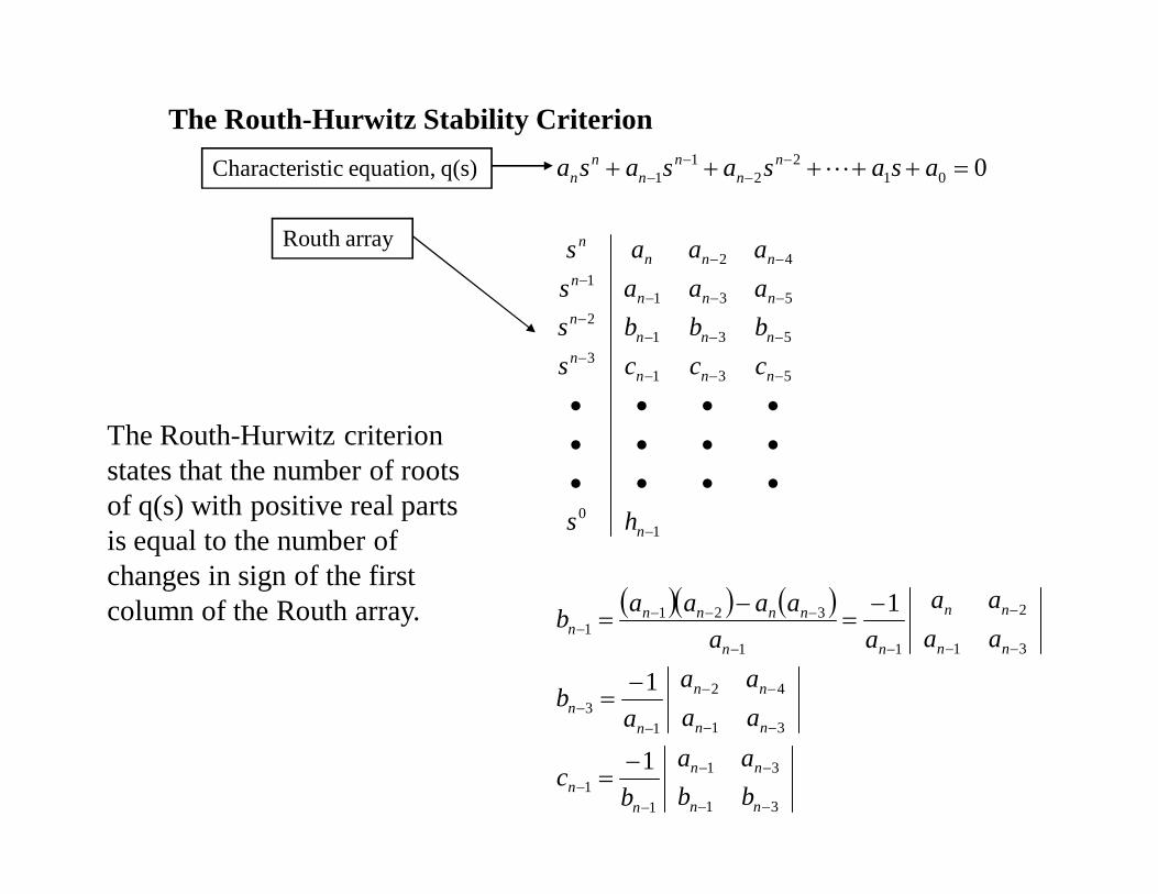
asasasasa Characteristic equation, q(s)
Routh array
The Routh-Hurwitz criterion states that the number of roots of q(s) with positive real parts is equal to the number of changes in sign of the first column of the Routh array.

The Routh-Hurwitz Stability CriterionCase One: No element in the first column is zero.
Example 6.1 Second-order system
The Characteristic polynomial of a second-order sys tem is:
q s( ) a2 s2 a1 s a0
The Routh array is written as:
w here:
b1a1 a0 0( ) a2
a1a0
Therefore the requirement for a stable second-order system is simply that all coef f icients be positive or all the coef ficients be negative.
00
10
11
022
bsas
aas
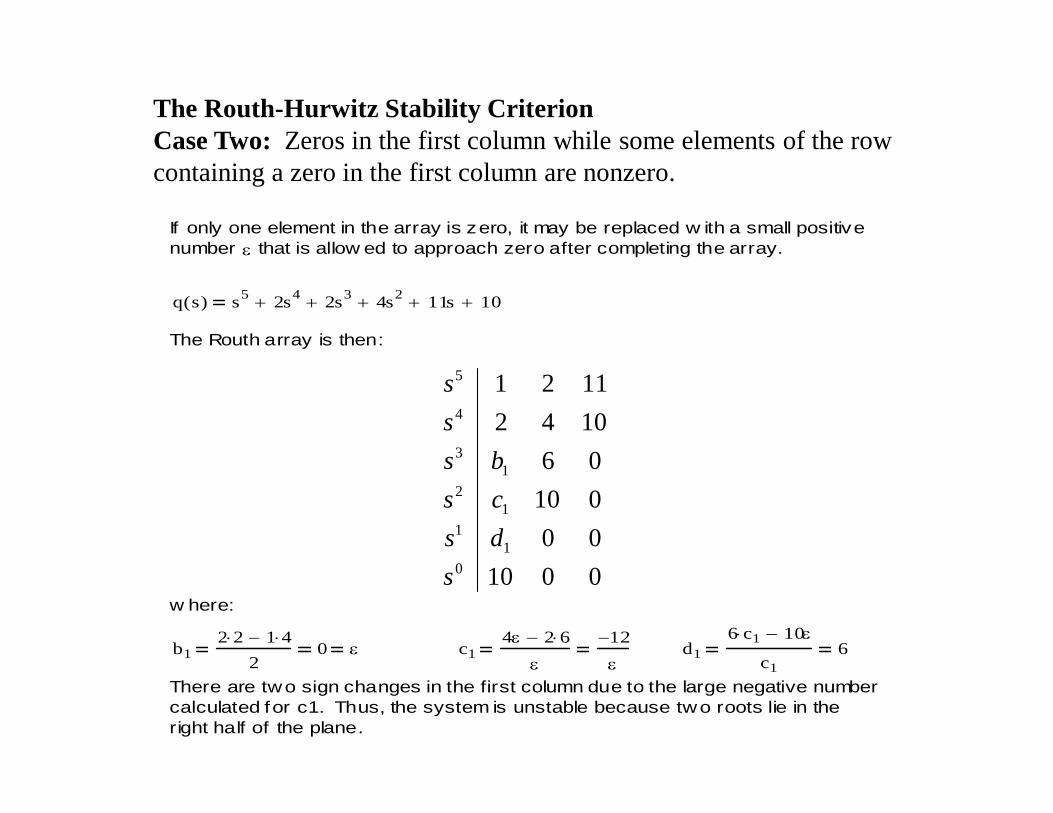
The Routh-Hurwitz Stability CriterionCase Two: Zeros in the first column while some elements of the row containing a zero in the first column are nonzero.
If only one element in the array is zero, it may be replaced w ith a small positive number that is allow ed to approach zero after completing the array.
q s( ) s5 2s4 2s3 4s2 11s 10
The Routh array is then:
w here:
b12 2 1 4
20 c1
4 2 6
12
d1
6 c1 10
c16
There are two sign changes in the first column due to the large negative number calculated for c1. Thus, the system is unstable because two roots lie in the right half of the plane.
00100001006
10421121
01
11
21
3
4
5
sdscsbs
ss

The Routh-Hurwitz Stability CriterionCase Three: Zeros in the first column, and the other elements of the row containing the zero are also zero.
This case occurs when the polynomial q(s) has zeros located symetrically about the origin of the s-plane, such as (s+)(s -) or (s+j)(s -j). This case is solved using the auxiliary polynomial, U(s), w hich is located in the row above the row containing the zero entry in the Routh array.
q s( ) s3 2 s2 4s K
Routh array:
For a stable system we require that 0 s 8
For the marginally stable case, K=8, the s^1 row of the Routh array contains all zeros. The auxiliary plynomial comes from the s^2 row .
U s( ) 2s2 Ks0 2 s2 8 2 s2 4 2 s j 2( ) s j 2( )
It can be proven that U(s) is a factor of the characteristic polynomial:
q s( )U s( )
s 2
2 Thus, w hen K=8, the factors of the characteristic polynomial are:
q s( ) s 2( ) s j 2( ) s j 2( )
00
241
02
81
2
3
Kss
Kss
K

The Routh-Hurwitz Stability CriterionCase Four: Repeated roots of the characteristic equation on the jw-axis.
With simple roots on the jw-axis, the system will have a marginally stable behavior. This is not the case if the roots are repeated. Repeated roots on the jw-axis will cause the system to be unstable. Unfortunately, the routh-array will fail to reveal this instability.
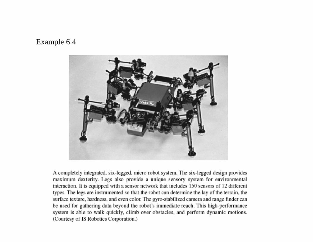
Example 6.4
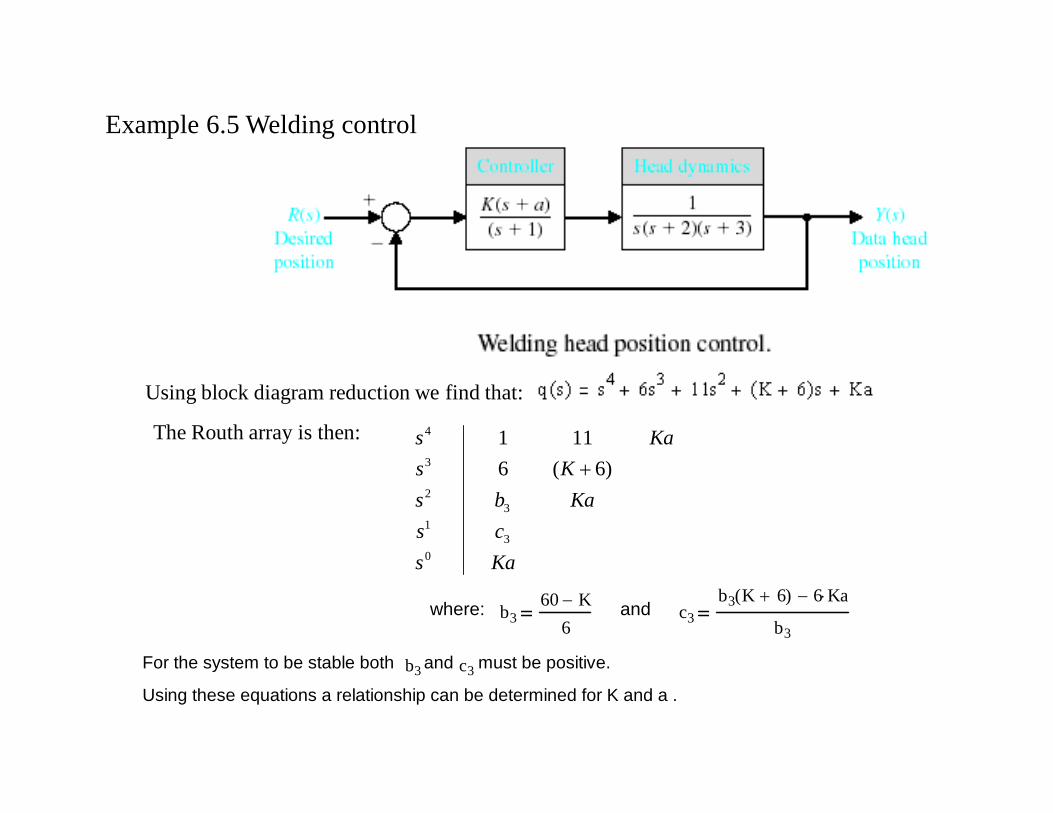
Example 6.5 Welding control
Using block diagram reduction we find that:
The Routh array is then:
Kascs
KabsKs
Kas
03
13
2
3
4
)6(6111
For the system to be stable both b3 and c3 must be positive.
Using these equations a relationship can be determined for K and a .
where: b360 K
6and c3
b3 K 6( ) 6 Ka
b3
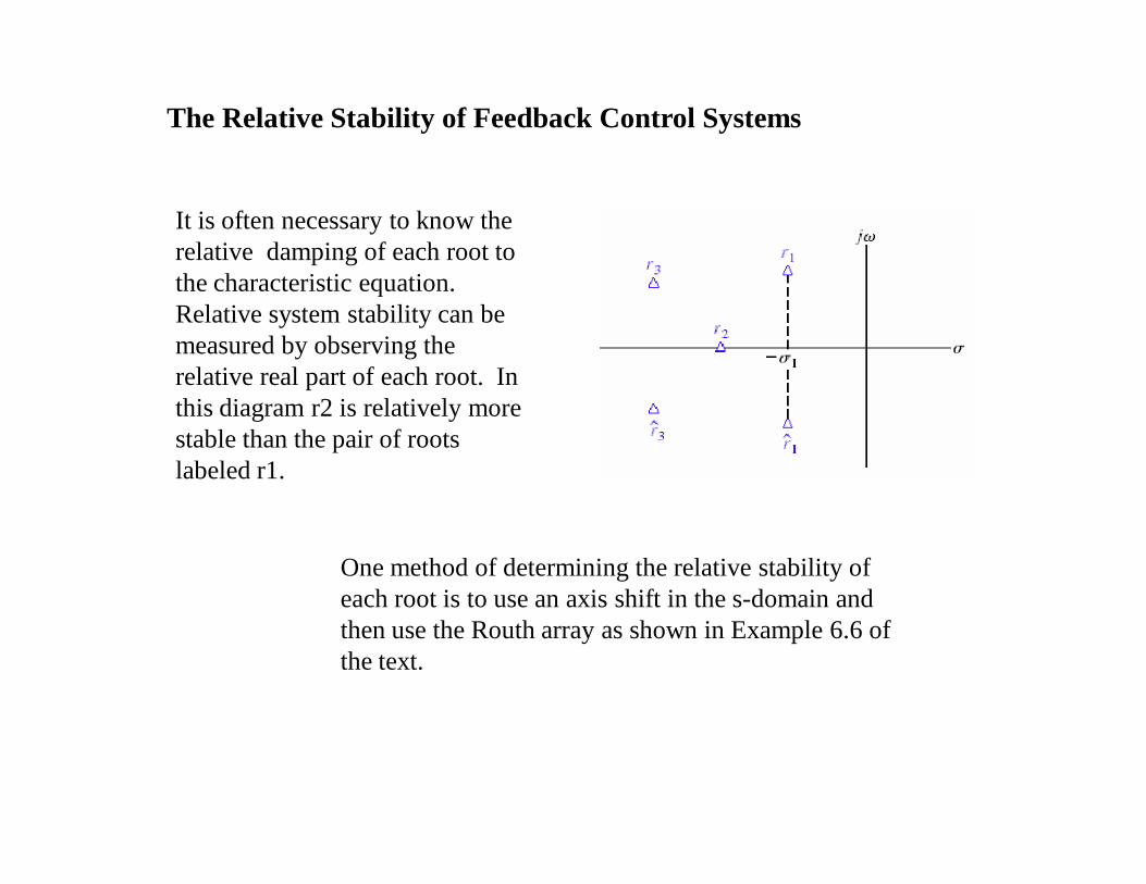
The Relative Stability of Feedback Control Systems
It is often necessary to know the relative damping of each root to the characteristic equation. Relative system stability can be measured by observing the relative real part of each root. In this diagram r2 is relatively more stable than the pair of roots labeled r1.
One method of determining the relative stability of each root is to use an axis shift in the s-domain and then use the Routh array as shown in Example 6.6 of the text.

Problem statement: Design the turning control for a tracked vehicle. Select K and a so that the system is stable. The system is modeled below.
Design Example: Tracked Vehicle Turning Control
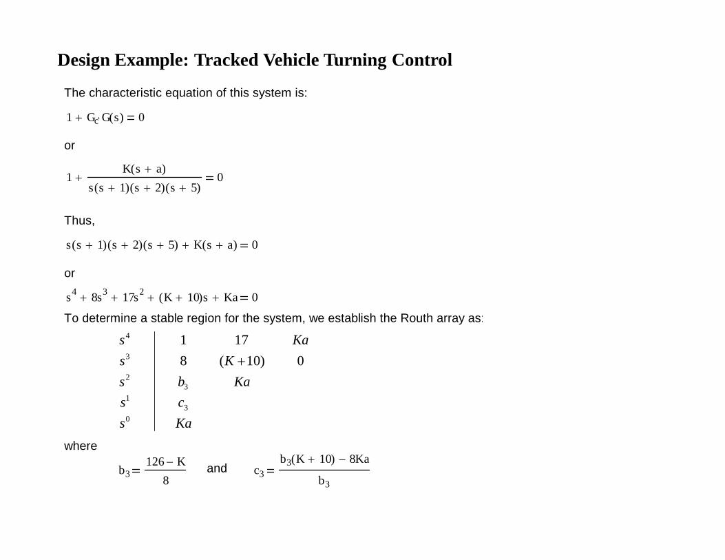
The characteristic equation of this system is:
1 Gc G s( ) 0
or
1K s a( )
s s 1( ) s 2( ) s 5( ) 0
Thus,
s s 1( ) s 2( ) s 5( ) K s a( ) 0
or
s4 8s3 17s2 K 10( )s Ka 0
To determine a stable region for the system, we establish the Routh array as:
where
b3126 K
8and c3
b3 K 10( ) 8Ka
b3
Kascs
KabsKs
Kas
03
13
2
3
4
0)10(8171
Design Example: Tracked Vehicle Turning Control

Kascs
KabsKs
Kas
03
13
2
3
4
0)10(8171
Design Example: Tracked Vehicle Turning Control
where
b3126 K
8and c3
b3 K 10( ) 8Ka
b3
Therefore,
K 126
K a 0
K 10( ) 126 K( ) 64Ka 0

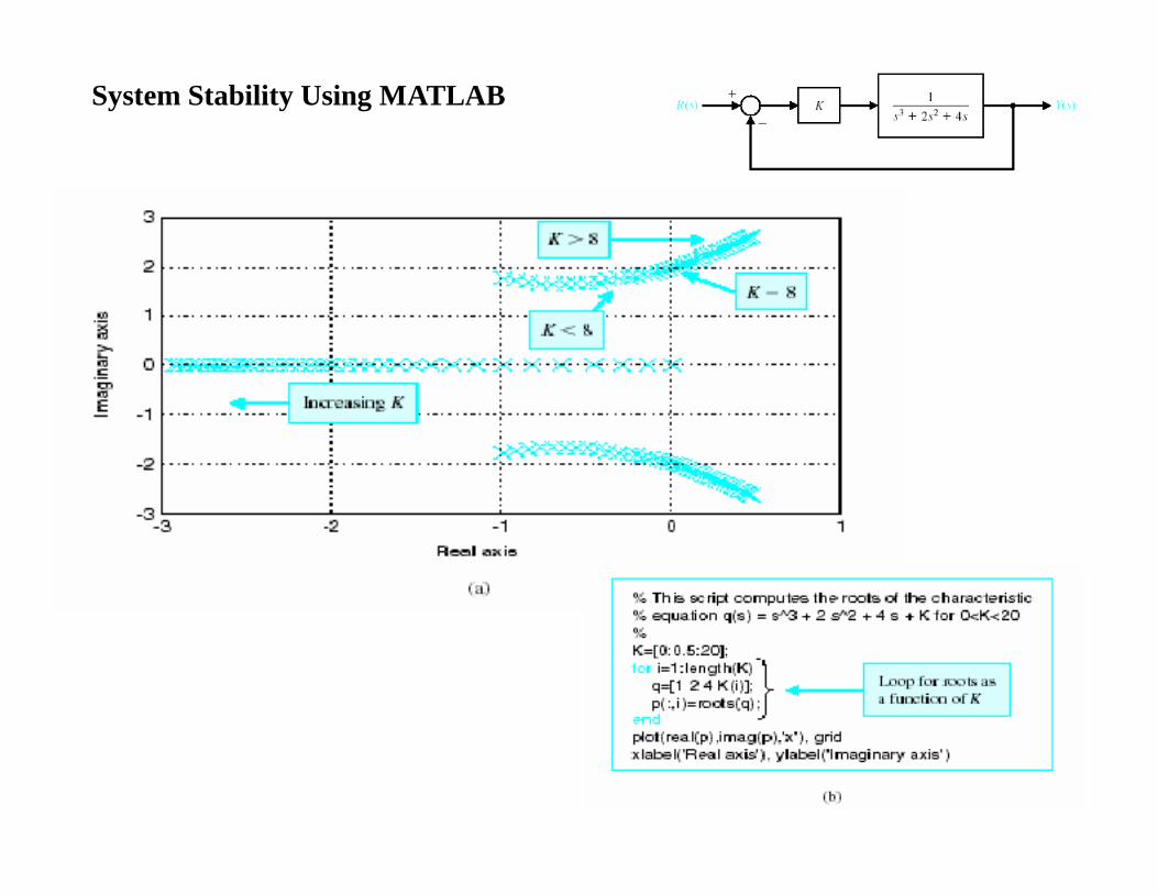
System Stability Using MATLAB
System Stability Using MATLAB
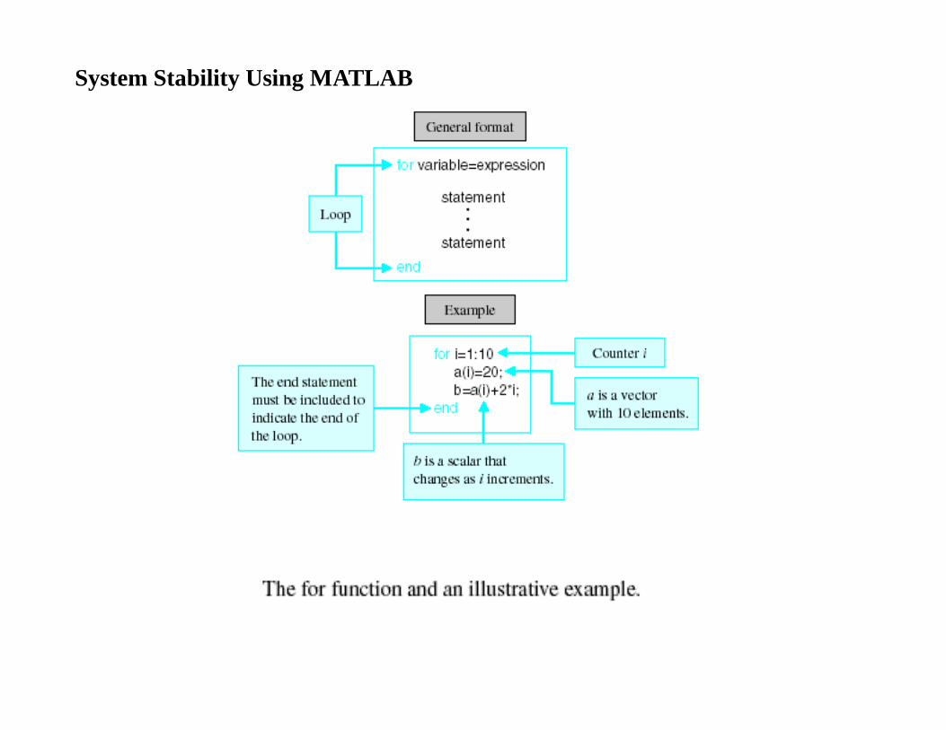
System Stability Using MATLAB

System Stability Using MATLAB

UNIT - IV
STABILITY IN FREQUENCY DOMAIN

Introduction
The frequency response of a system is defined as the steady-state response of the system to a sinusoidal input signal. The sinusoid is a unique input signal, and the resulting output signal for a linear system, as well as signals throughout the system, is sinusoidal in the steady-state; it differs form the input waveform only in amplitude and phase.

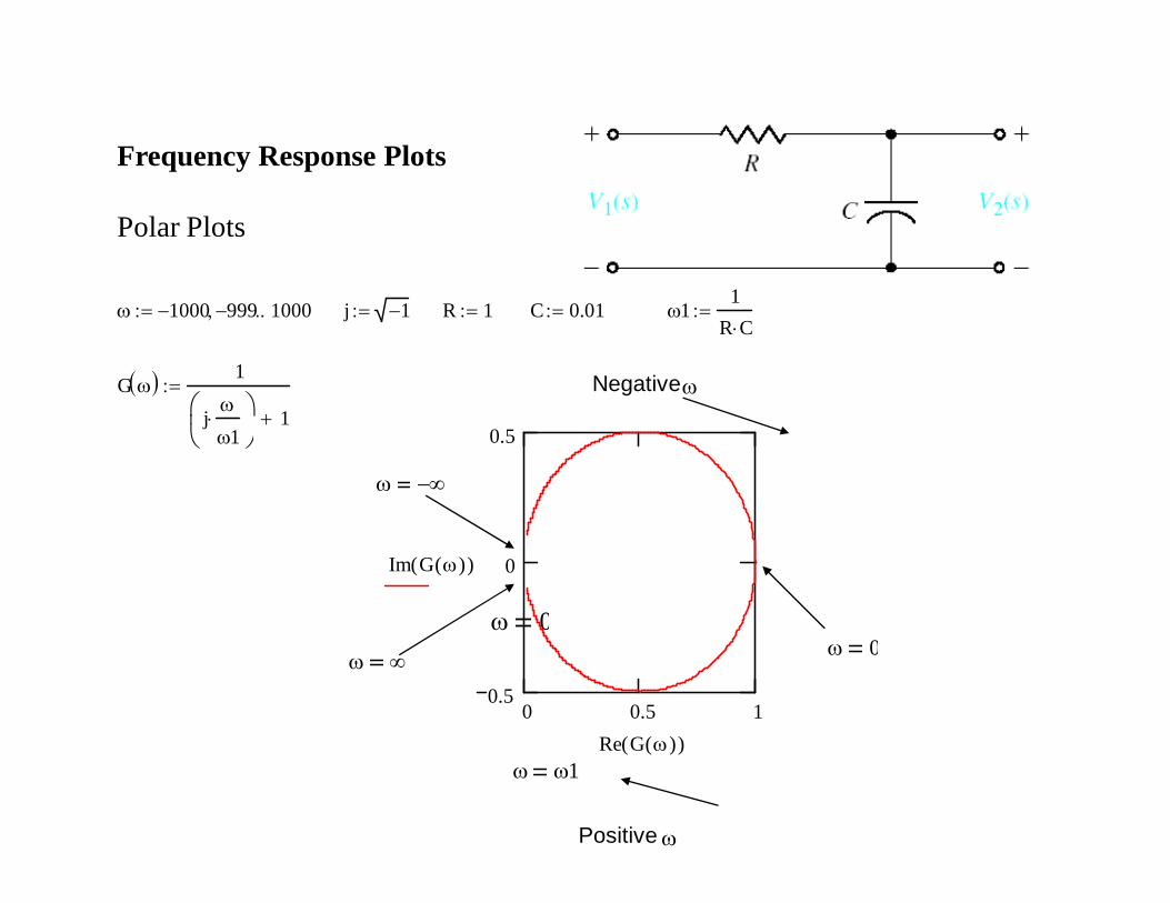
Frequency Response Plots
Polar Plots
Frequency Response Plots
Polar Plots
0
1000 999 1000 j 1 R 1 C 0.01 11
R C
G 1
j
1
1
Negative
0 0.5 10.5
0
0.5
Im G ( )( )
Re G ( )( )
0
1
Positive
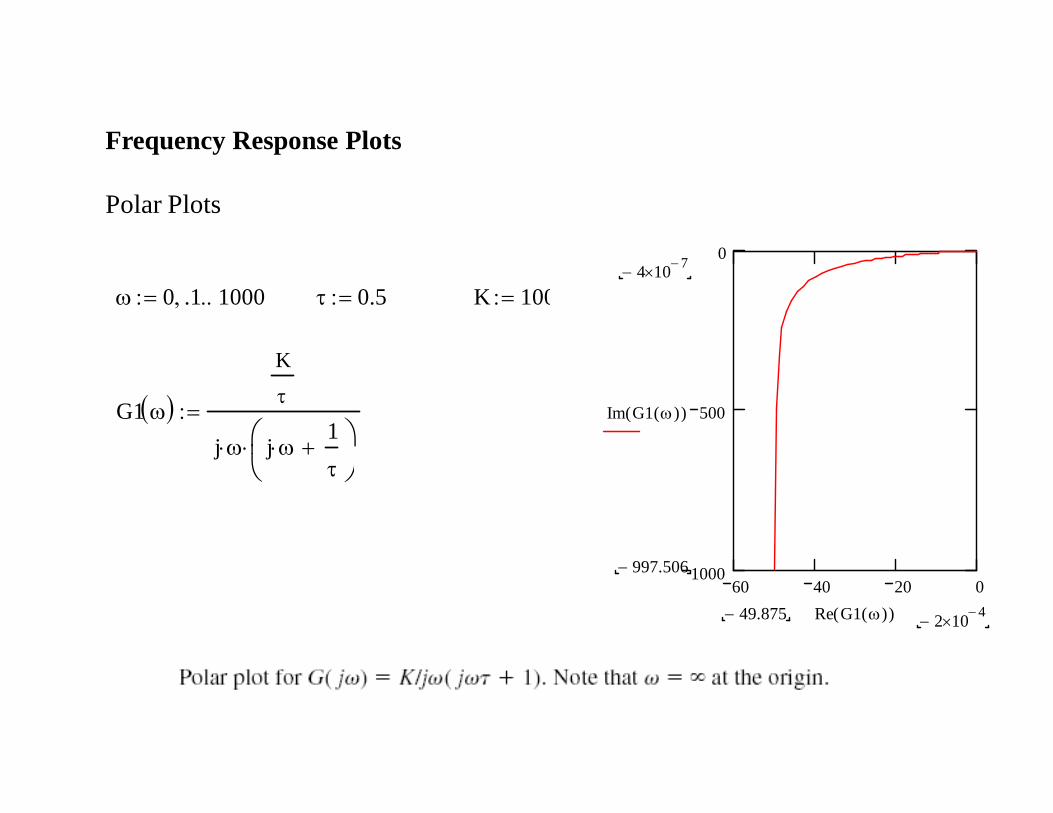
Frequency Response Plots
Polar Plots
60 40 20 01000
500
04 10 7
997.506
Im G1 ( )( )
2 10 449.875 Re G1 ( )( )
0 .1 1000 0.5 K 100
G1
K
j j 1
Frequency Response Plots
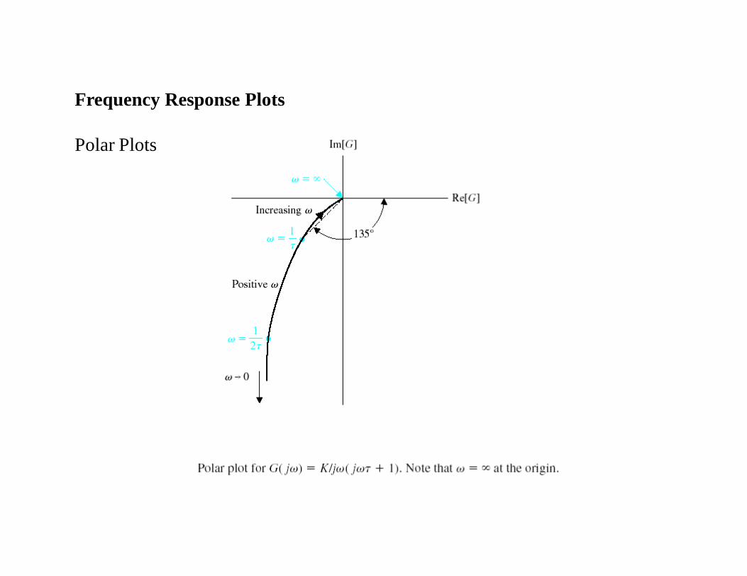
Polar Plots

Frequency Response Plots
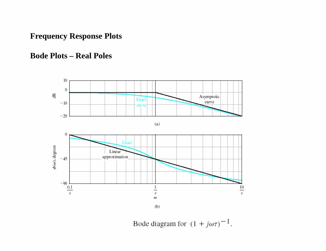
Bode Plots – Real Poles

Frequency Response Plots
Bode Plots – Real Poles
0.1
0.11
1000 j 1 R 1 C 0.01 R C
11
1 100G 1j 1
0.1 1 10 100 1 10330
20
10
0
20 log G ( )
(break frequency or corner frequency)
(break frequency or corner frequency)
-3dB

Frequency Response Plots
Bode Plots – Real Poles
atan
0.1 1 10 100 1 1031.5
1
0.5
0
( )
(break frequency or corner frequency)
Frequency Response Plots
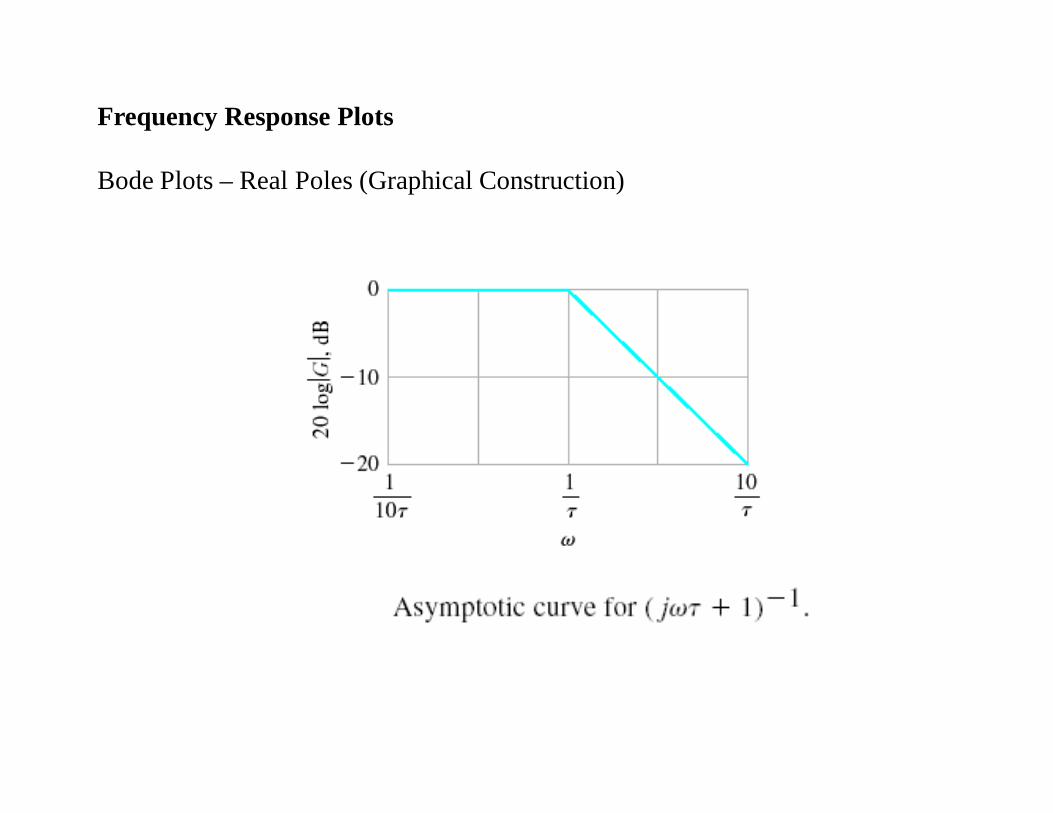
Bode Plots – Real Poles (Graphical Construction)

Frequency Response Plots
Bode Plots – Real Poles
Frequency Response Plots
Bode Plots – Real Poles

si j ii end 10i rrange variable:i 0 Nrange for plot:
r logstart
end
1Nstep size:
end 100highest frequency (in Hz):
N 50number of points:start .01lowest frequency (in Hz):
Next, choose a frequency range for the plots (use powers of 10 for convenient plotting):
G s( )K
s 1 s( ) 1s3
K 2
Assume
ps G 180
arg G j 360 if arg G j 0 1 0
Phase shift:
db G 20 log G j
Magnitude:
Frequency Response Plots
Bode Plots – Real Poles
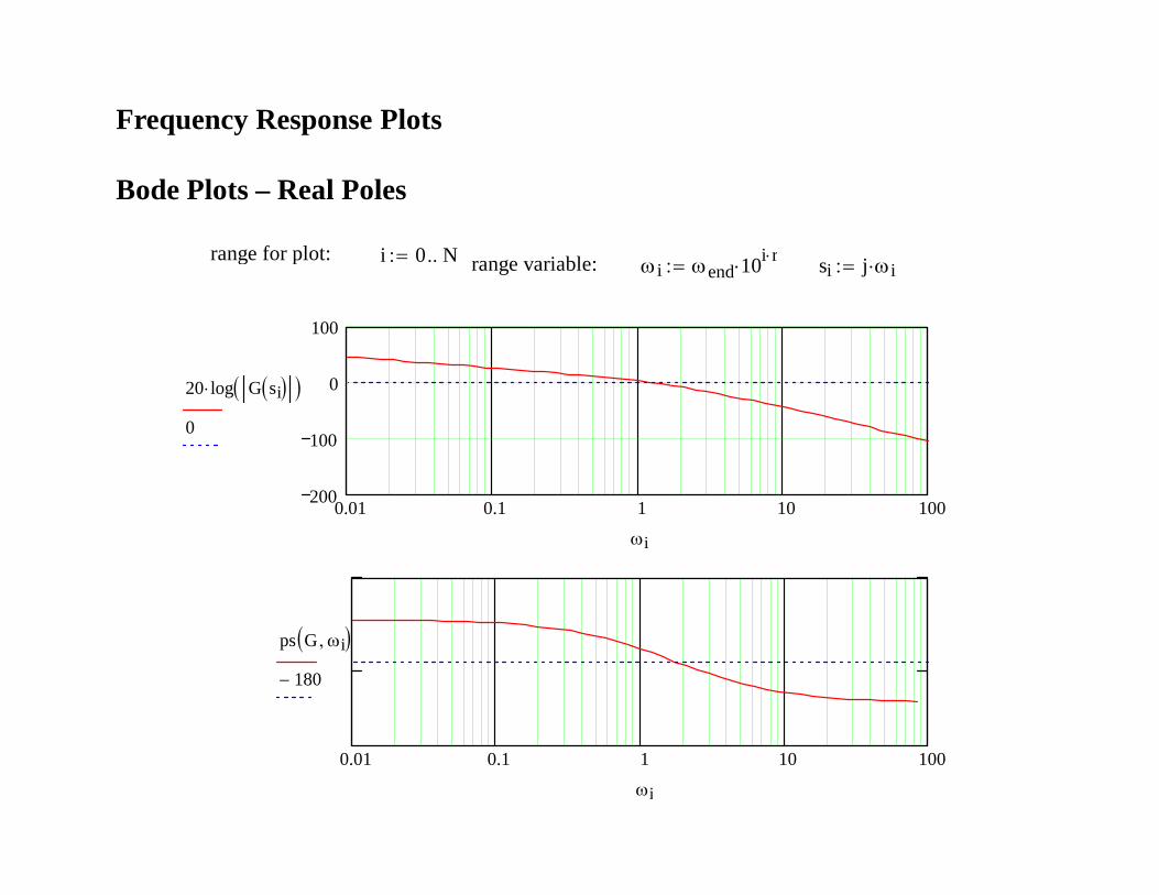
range for plot: i 0 N range variable: i end 10i r si j i
0.01 0.1 1 10 100200
100
0
100
20 log G si
0
i
0.01 0.1 1 10 100
ps G i 180
i
Frequency Response Plots
Bode Plots – Real Poles

Frequency Response Plots
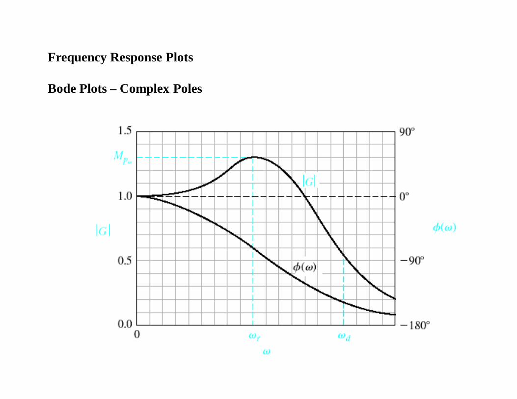
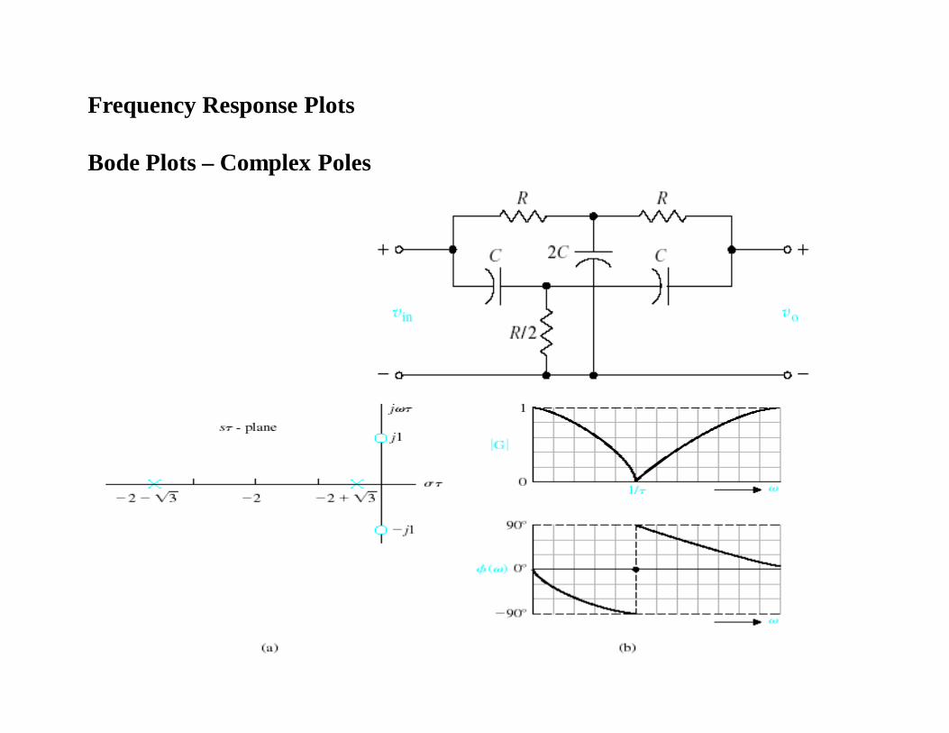
Bode Plots – Complex Poles

Frequency Response Plots
Bode Plots – Complex Poles

Frequency Response Plots
Bode Plots – Complex Poles
r n 1 2 2
0.707
Mp G r 1
2 1 2
0.707

Frequency Response Plots
Bode Plots – Complex Poles
r n 1 2 2
0.707
Mp G r 1
2 1 2
0.707
Frequency Response Plots
Bode Plots – Complex Poles
Frequency Response Plots
Bode Plots – Complex Poles

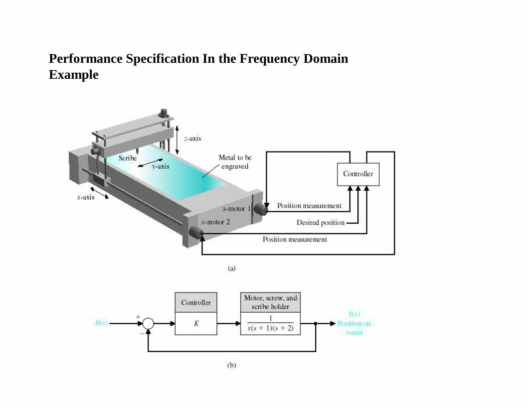
Performance Specification In the Frequency Domain
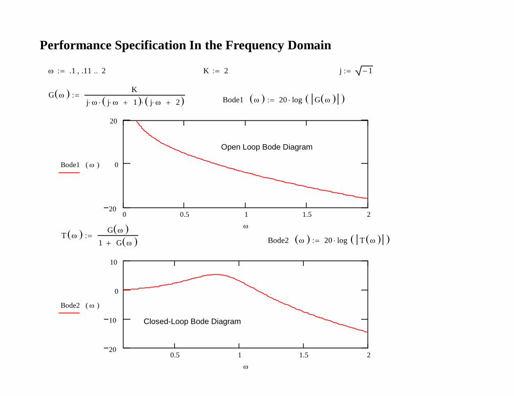
.1 .11 2 K 2 j 1
G Kj j 1 j 2
Bode1 20 log G
0 0.5 1 1.5 220
0
20
Bode1 ( )
Open Loop Bode Diagram
T G 1 G
Bode2 20 log T
0.5 1 1.5 220
10
0
10
Bode2 ( )
Closed-Loop Bode Diagram
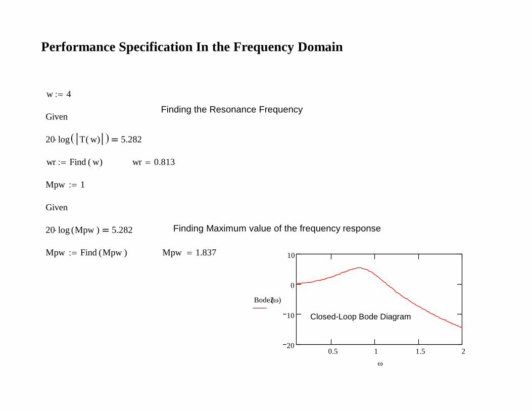
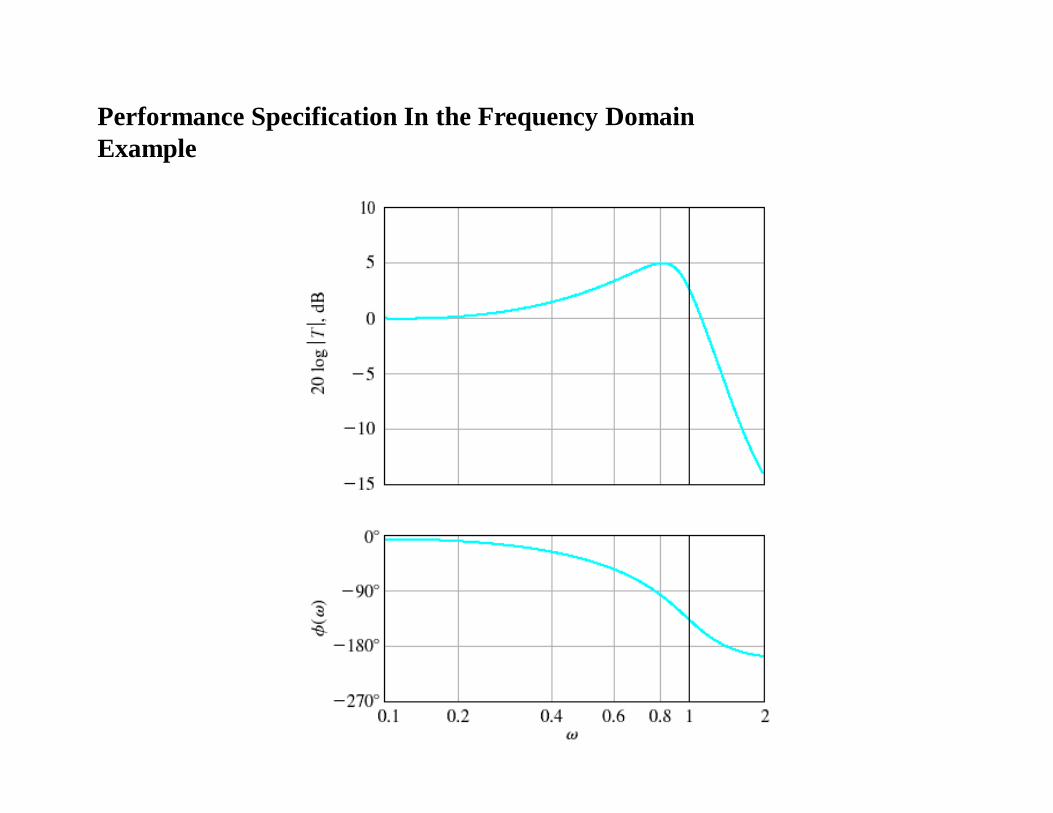
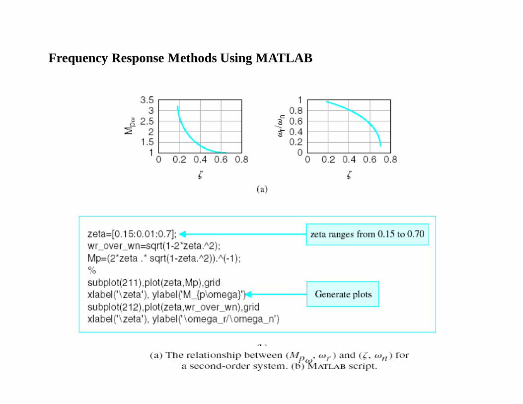
Performance Specification In the Frequency Domain
Performance Specification In the Frequency Domain
w 4
Finding the Resonance FrequencyGiven
20 log T w( ) 5.282
wr Find w( ) wr 0.813
Mpw 1
Given
20 log Mpw( ) 5.282 Finding Maximum value of the frequency response
Mpw Find Mpw( ) Mpw 1.837
0.5 1 1.5 220
10
0
10
Bode2( )
Closed-Loop Bode Diagram

Assume that the system has dominant second-order roots
.1 Finding the damping factorGiven
Mpw 2 1 2
1
Find 0.284
wn .1 Finding the natural frequency
Given
wr wn 1 2 2
wn Find wn( ) wn 0.888
Performance Specification In the Frequency Domain
0.5 1 1.5 220
10
0
10
Bode2( )
Closed-Loop Bode Diagram

Performance Specification In the Frequency Domain
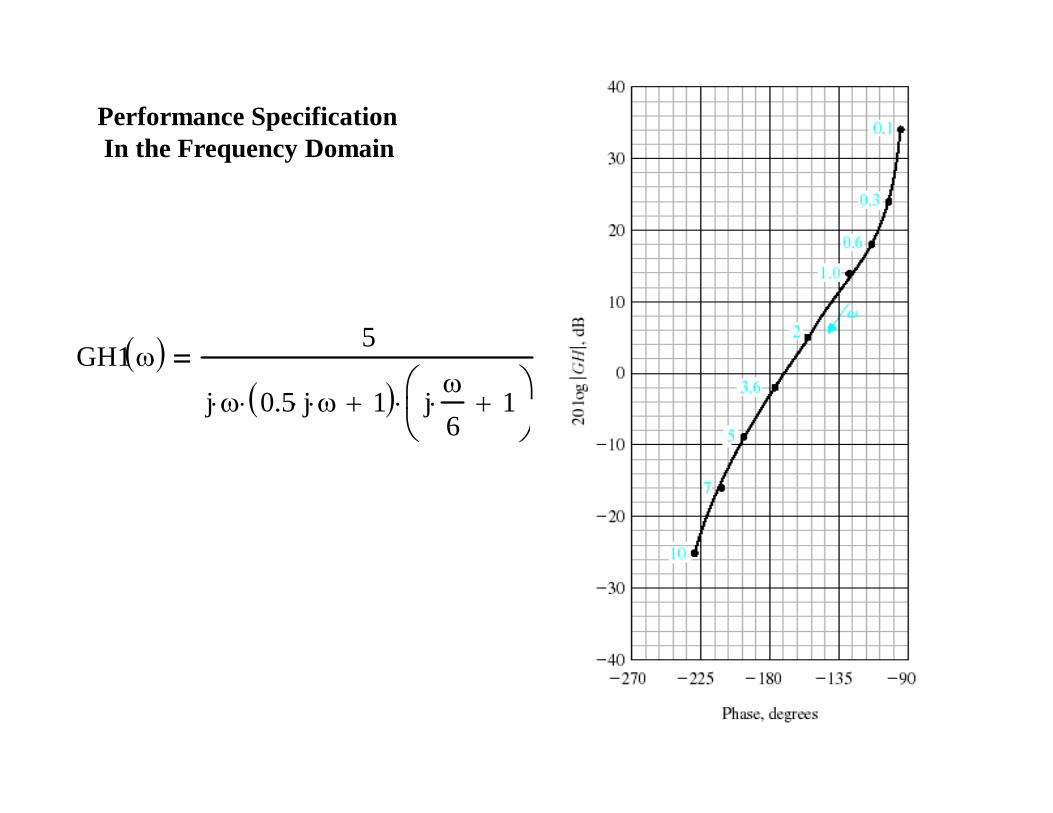
Performance SpecificationIn the Frequency Domain
GH1 5
j 0.5 j 1 j
6 1
Performance Specification In the Frequency DomainExample

Performance Specification In the Frequency DomainExample

Performance Specification In the Frequency DomainExample
Performance Specification In the Frequency DomainExample

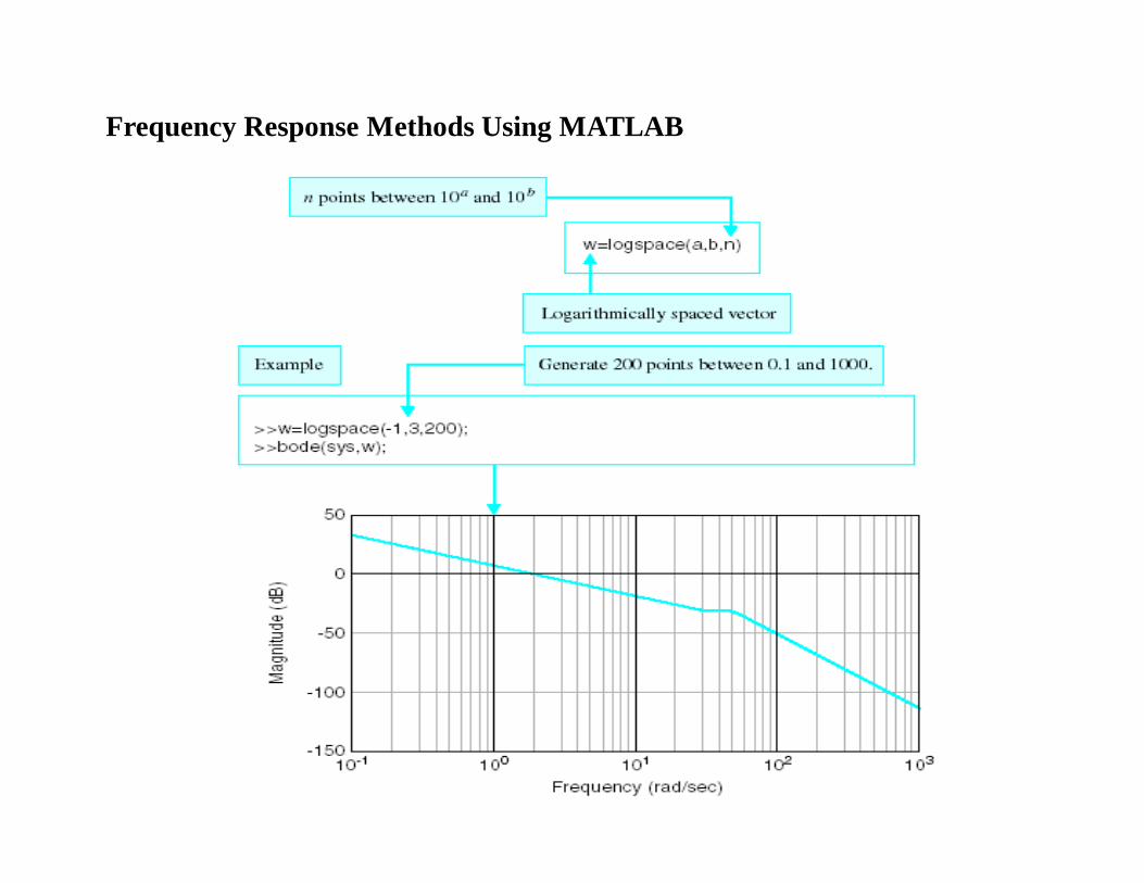
Frequency Response Methods Using MATLAB

Frequency Response Methods Using MATLAB
Frequency Response Methods Using MATLAB
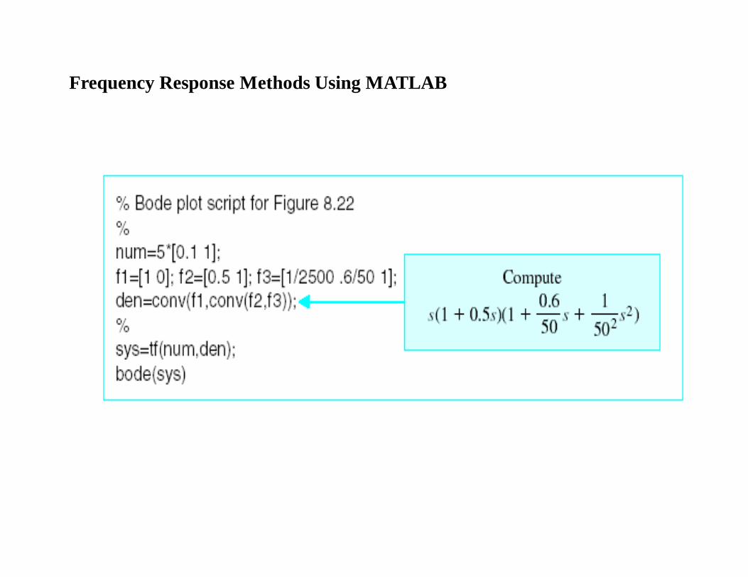
Frequency Response Methods Using MATLAB
Frequency Response Methods Using MATLAB
Frequency ResponseMethods Using MATLAB

Frequency ResponseMethods Using MATLAB

Bode Plots
Bode plot is the representation of the magnitude and phase of G(j*w) (where the frequency vector w contains only positive frequencies). To see the Bode plot of a transfer function, you can use the MATLAB bodecommand.
For example,
bode(50,[1 9 30 40])
displays the Bode plots for the transfer function:
50 / (s^3 + 9 s^2 + 30 s + 40)
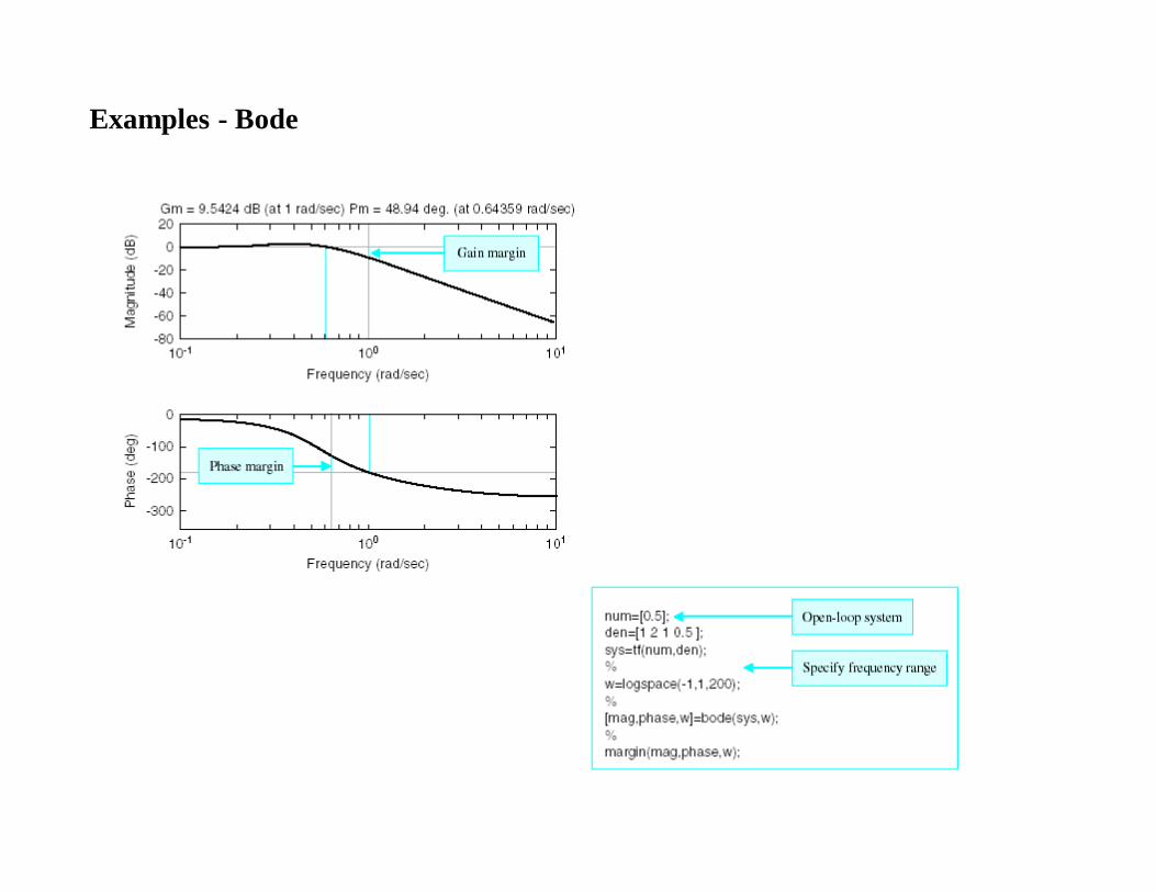
Gain and Phase Margin
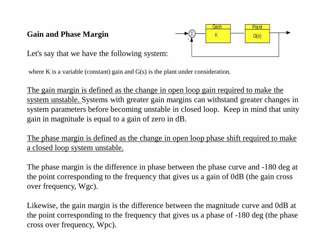
Let's say that we have the following system:
where K is a variable (constant) gain and G(s) is the plant under consideration.
The gain margin is defined as the change in open loop gain required to make the system unstable. Systems with greater gain margins can withstand greater changes in system parameters before becoming unstable in closed loop. Keep in mind that unity gain in magnitude is equal to a gain of zero in dB.
The phase margin is defined as the change in open loop phase shift required to make a closed loop system unstable.
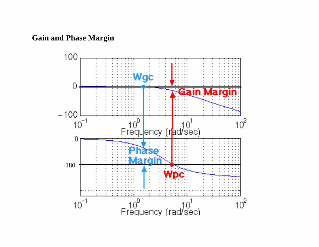
The phase margin is the difference in phase between the phase curve and -180 deg at the point corresponding to the frequency that gives us a gain of 0dB (the gain cross over frequency, Wgc).
Likewise, the gain margin is the difference between the magnitude curve and 0dB at the point corresponding to the frequency that gives us a phase of -180 deg (the phase cross over frequency, Wpc).
Gain and Phase Margin
-180
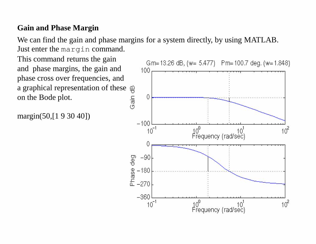
We can find the gain and phase margins for a system directly, by using MATLAB. Just enter the margin command. This command returns the gain and phase margins, the gain and phase cross over frequencies, and a graphical representation of these on the Bode plot.
margin(50,[1 9 30 40])
Gain and Phase Margin
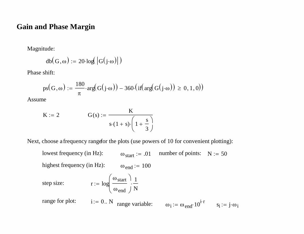
si j ii end 10i rrange variable:i 0 Nrange for plot:
r logstart
end
1Nstep size:
end 100highest frequency (in Hz):
N 50number of points:start .01lowest frequency (in Hz):
Next, choose a frequency range for the plots (use powers of 10 for convenient plotting):
G s( )K
s 1 s( ) 1s3
K 2
Assume
ps G 180
arg G j 360 if arg G j 0 1 0
Phase shift:
db G 20 log G j
Magnitude:
Gain and Phase Margin
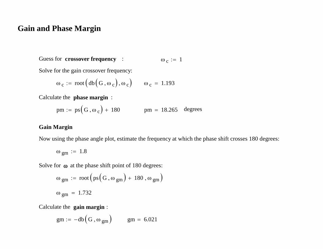
gm 6.021gm db G gm
Calculate the gain margin :
gm 1.732
gm root ps G gm 180 gm
Solve for at the phase shift point of 180 degrees:
gm 1.8
Now using the phase angle plot, estimate the frequency at which the phase shift crosses 180 degrees:
Gain Margin
degreespm 18.265pm ps G c 180
Calculate the phase margin :
c 1.193 c root db G c c
Solve for the gain crossover frequency:
c 1Guess for crossover frequency :
Gain and Phase Margin
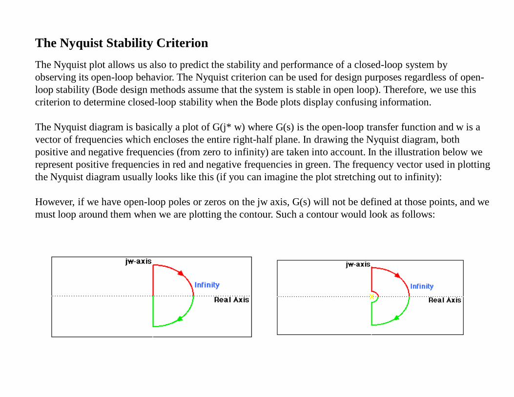
The Nyquist Stability CriterionThe Nyquist plot allows us also to predict the stability and performance of a closed-loop system by observing its open-loop behavior. The Nyquist criterion can be used for design purposes regardless of open-loop stability (Bode design methods assume that the system is stable in open loop). Therefore, we use this criterion to determine closed-loop stability when the Bode plots display confusing information.
The Nyquist diagram is basically a plot of G(j* w) where G(s) is the open-loop transfer function and w is a vector of frequencies which encloses the entire right-half plane. In drawing the Nyquist diagram, both positive and negative frequencies (from zero to infinity) are taken into account. In the illustration below we represent positive frequencies in red and negative frequencies in green. The frequency vector used in plotting the Nyquist diagram usually looks like this (if you can imagine the plot stretching out to infinity):
However, if we have open-loop poles or zeros on the jw axis, G(s) will not be defined at those points, and we must loop around them when we are plotting the contour. Such a contour would look as follows:

The Cauchy criterion
The Cauchy criterion (from complex analysis) states that when taking a closed contour in the complex plane, and mapping it through a complex function G(s), the number of times that the plot of G(s) encircles the origin is equal to the number of zeros of G(s) enclosed by the frequency contour minus the number of poles of G(s) enclosed by the frequency contour. Encirclements of the origin are counted as positive if they are in the same direction as the original closed contour or negative if they are in the opposite direction.
When studying feedback controls, we are not as interested in G(s) as in the closed-loop transfer function:
G(s)---------1 + G(s)
If 1+ G(s) encircles the origin, then G(s) will enclose the point -1. Since we are interested in the closed-loop stability, we want to know if there are any closed-loop poles (zeros of 1 + G(s)) in the right-half plane.
Therefore, the behavior of the Nyquist diagram around the -1 point in the real axis is very important; however, the axis on the standard nyquist diagram might make it hard to see what's happening around this point

Gain and Phase Margin
Gain Margin is defined as the change in open-loop gain expressed in decibels (dB), required at 180 degrees of phase shift to make the system unstable. First of all, let's say that we have a system that is stable if there are no Nyquist encirclements of -1, such as :
50-----------------------
s^3 + 9 s^2 + 30 s + 40
Looking at the roots, we find that we have no open loop poles in the right half plane and therefore no closed-loop poles in the right half plane if there are no Nyquist encirclements of -1. Now, how much can we vary the gain before this system becomes unstable in closed loop?
The open-loop system represented by this plot will become unstable in closed loop if the gain is increased past a certain boundary.
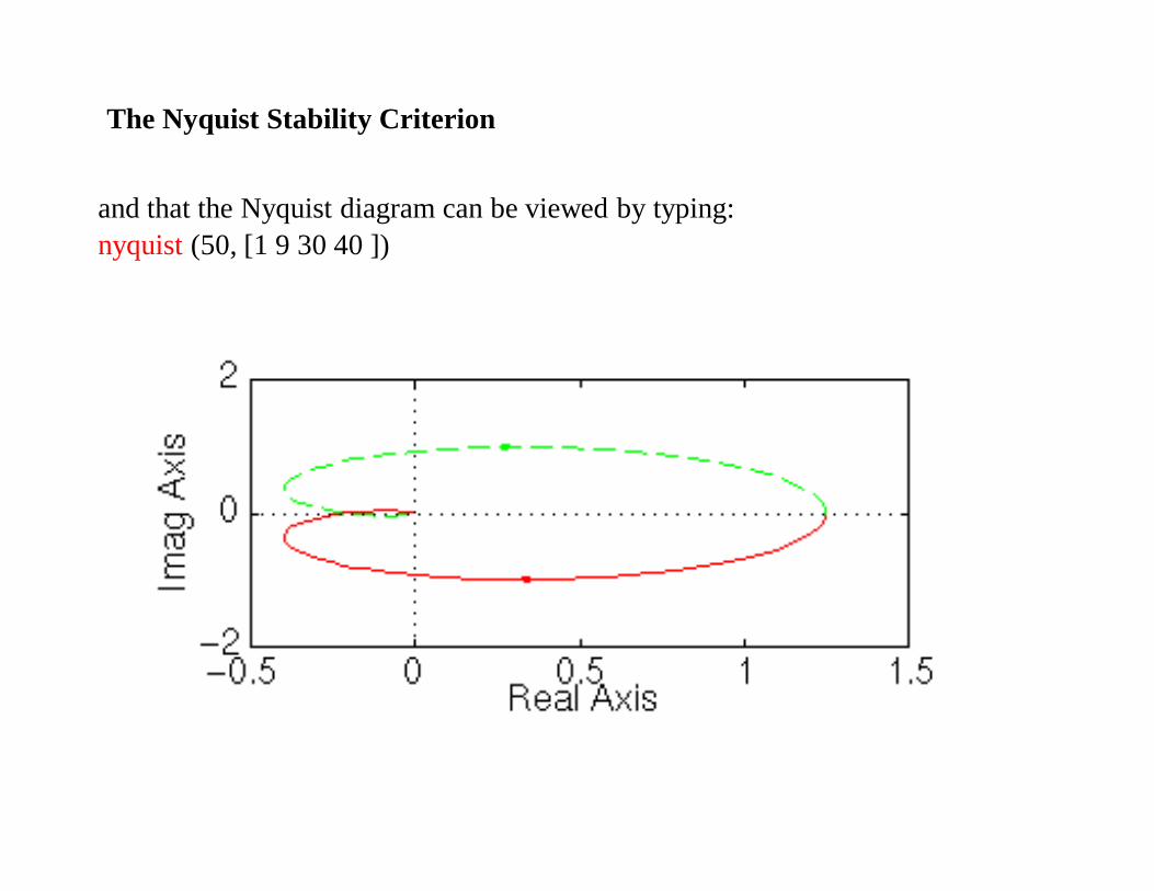
and that the Nyquist diagram can be viewed by typing: nyquist (50, [1 9 30 40 ])
The Nyquist Stability Criterion
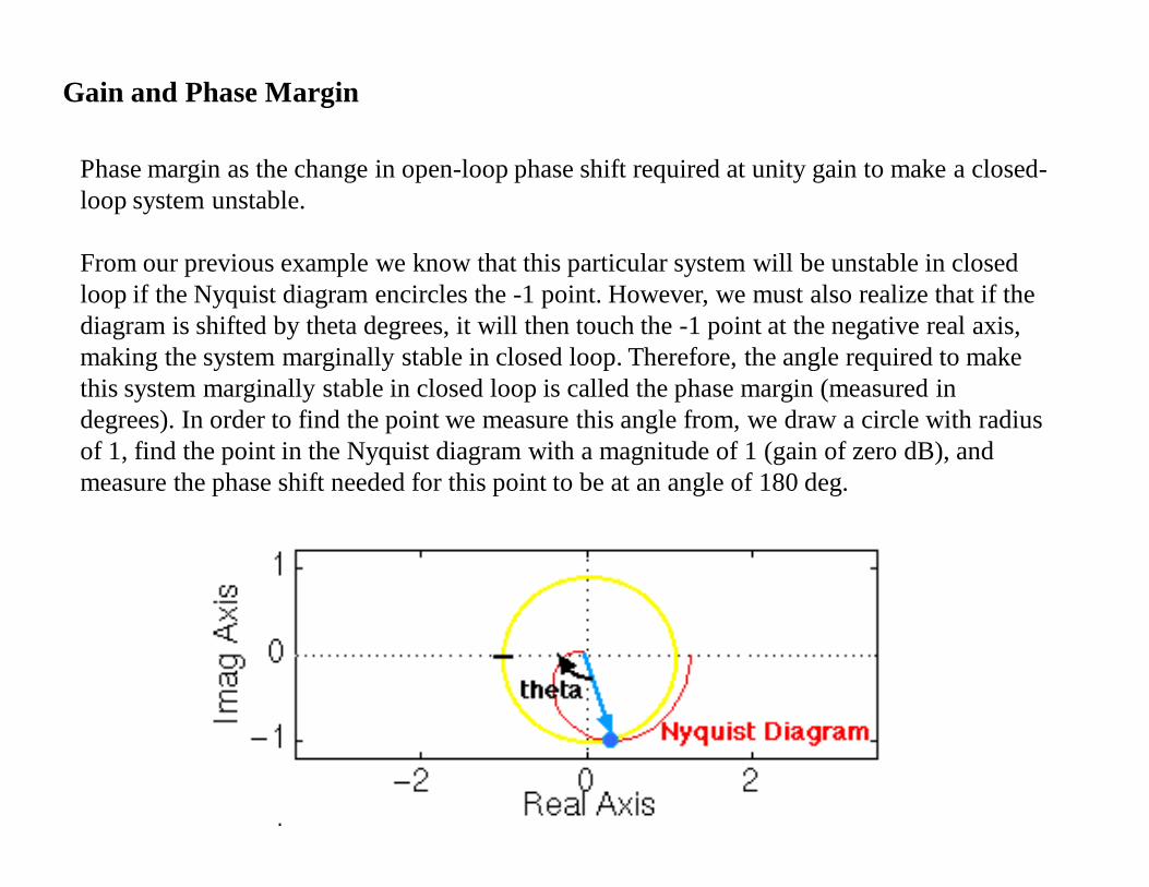
Phase margin as the change in open-loop phase shift required at unity gain to make a closed-loop system unstable.
From our previous example we know that this particular system will be unstable in closed loop if the Nyquist diagram encircles the -1 point. However, we must also realize that if the diagram is shifted by theta degrees, it will then touch the -1 point at the negative real axis, making the system marginally stable in closed loop. Therefore, the angle required to make this system marginally stable in closed loop is called the phase margin (measured in degrees). In order to find the point we measure this angle from, we draw a circle with radius of 1, find the point in the Nyquist diagram with a magnitude of 1 (gain of zero dB), and measure the phase shift needed for this point to be at an angle of 180 deg.
Gain and Phase Margin

w 100 99.9 100 j 1 s w( ) j w f w( ) 1
G w( )50 4.6
s w( )3 9 s w( )2 30 s w( ) 40
2 1 0 1 2 3 4 5 65
0
5
Im G w( )( )
0
Re G w( )( )
The Nyquist Stability Criterion

Consider the Negative Feedback System
Remember from the Cauchy criterion that the number N of times that the plot of G(s)H(s) encircles -1 is equal to the number Z of zeros of 1 + G(s)H(s) enclosed by the frequency contour minus the number P of poles of 1 + G(s)H(s) enclosed by the frequency contour (N = Z - P).
Keeping careful track of open- and closed-loop transfer functions, as well as numerators and denominators, you should convince yourself that:
the zeros of 1 + G(s)H(s) are the poles of the closed-loop transfer function
the poles of 1 + G(s)H(s) are the poles of the open-loop transfer function.
The Nyquist criterion then states that:
P = the number of open-loop (unstable) poles of G(s)H(s)
N = the number of times the Nyquist diagram encircles -1
clockwise encirclements of -1 count as positive encirclements
counter-clockwise (or anti-clockwise) encirclements of -1 count as negative encirclements
Z = the number of right half-plane (positive, real) poles of the closed-loop system
The important equation which relates these three quantities is:
Z = P + N
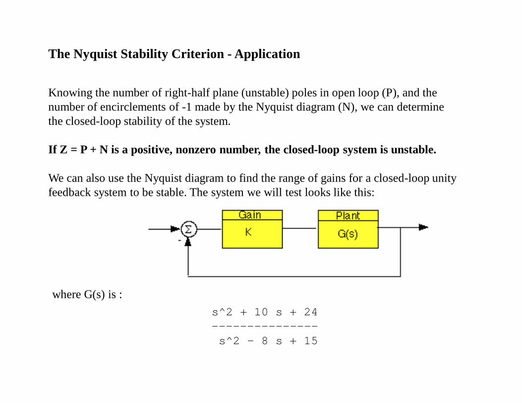
Knowing the number of right-half plane (unstable) poles in open loop (P), and the number of encirclements of -1 made by the Nyquist diagram (N), we can determine the closed-loop stability of the system.
If Z = P + N is a positive, nonzero number, the closed-loop system is unstable.
We can also use the Nyquist diagram to find the range of gains for a closed-loop unity feedback system to be stable. The system we will test looks like this:
where G(s) is :s^2 + 10 s + 24---------------s^2 - 8 s + 15
The Nyquist Stability Criterion - Application

This system has a gain K which can be varied in order to modify the response of the closed-loop system. However, we will see that we can only vary this gain within certain limits, since we have to make sure that our closed-loop system will be stable. This is what we will be looking for: the range of gains that will make this system stable in the closed loop.
The first thing we need to do is find the number of positive real poles in our open-loop transfer function:
roots([1 -8 15])ans =53
The poles of the open-loop transfer function are both positive. Therefore, we need two anti-clockwise (N = -2) encirclements of the Nyquist diagram in order to have a stable closed-loop system (Z = P + N). If the number of encirclements is less than two or the encirclements are not anti-clockwise, our system will be unstable.
Let's look at our Nyquist diagram for a gain of 1:
nyquist([ 1 10 24], [ 1 -8 15])
There are two anti-clockwise encirclements of -1. Therefore, the system is stable for a gain of 1.
The Nyquist Stability Criterion

MathCAD Implementation
w 100 99.9 100 j 1 s w( ) j w
G w( )s w( )2 10 s w( ) 24
s w( )2 8 s w( ) 15
2 1 0 1 22
0
2
Im G w( )( )
0
Re G w( )( )
The Nyquist Stability Criterion
There are two anti-clockwise encirclements of -1. Therefore, the system is stable for a gain of 1.

The Nyquist Stability Criterion
Time-Domain Performance Criteria SpecifiedIn The Frequency Domain
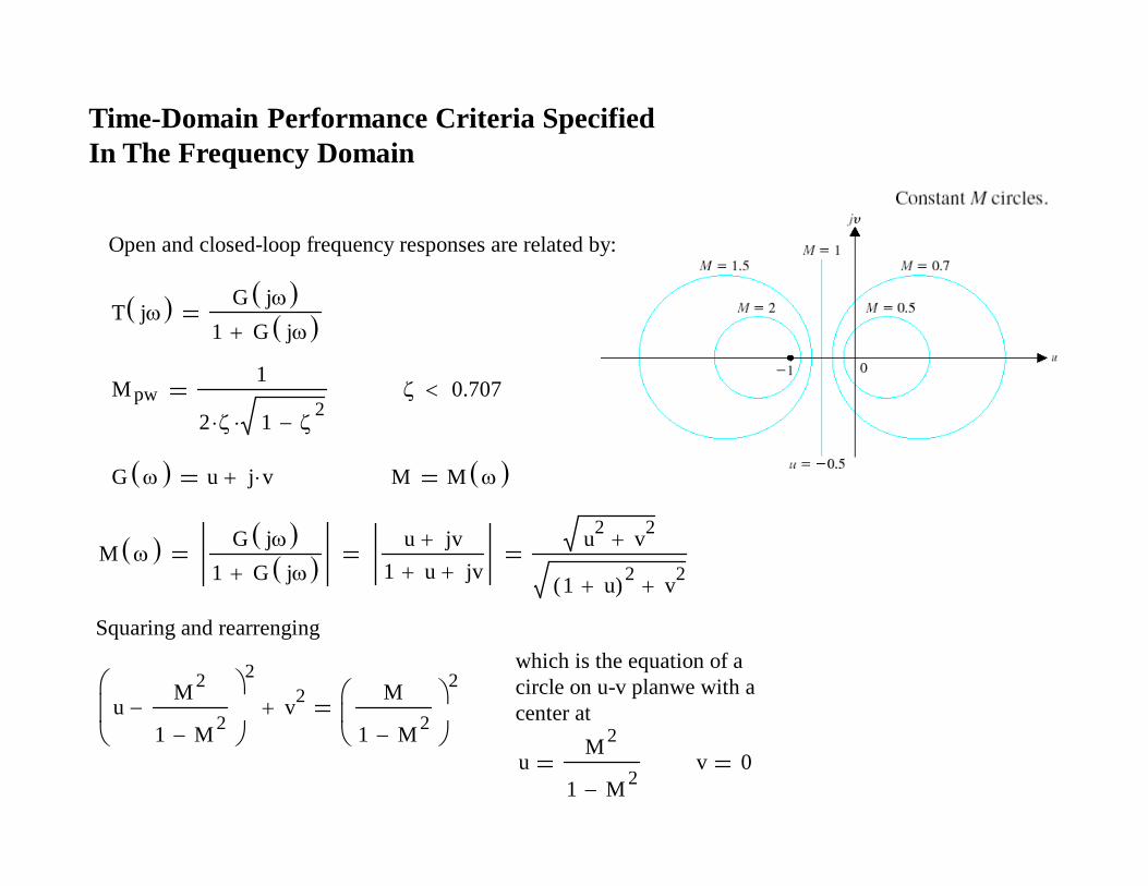
Open and closed-loop frequency responses are related by:
T j G j 1 G j
M pw1
2 1 2
0.707
G u j v M M
M G j 1 G j
u jv1 u jv
u2 v2
1 u( )2 v2
Squaring and rearrengingwhich is the equation of a circle on u-v planwe with a center atu
M 2
1 M 2
2
v2M
1 M 2
2
uM 2
1 M 2v 0

Time-Domain Performance Criteria SpecifiedIn The Frequency Domain

The Nichols Stability Method
Polar Stability Plot - Nichols Mathcad Implementation
This example makes a polar plot of a transfer function and draws one contour of constant closed-loop magnitude. To draw the plot, enter a definition for the transfer function G(s):
G s( )45000
s s 2( ) s 30( )
The frequency range defined by the next two equations provides a logarithmic frequency scale running from 1 to 100. You can change this range by editing the definitions for m and m:
m 0 100 m 10 .02 m
Now enter a value for M to define the closed-loop magnitude contour that will be plotted. M 1.1
Calculate the points on the M-circle:
MC mM2
M2 1
M
M2 1exp 2 j .01 m
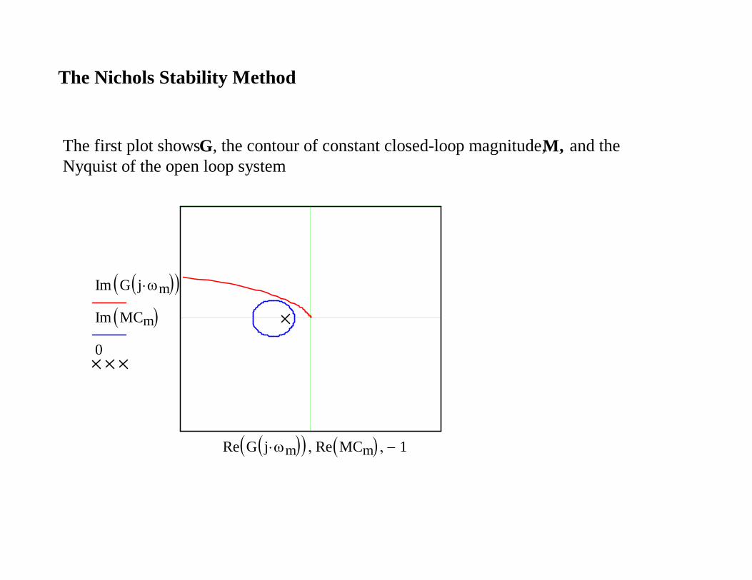
The first plot shows G, the contour of constant closed-loop magnitude, M
The Nichols Stability Method
The first plot shows G, the contour of constant closed-loop magnitude, M, and the Nyquist of the open loop system
Im G j m Im MCm 0
Re G j m Re MCm 1

The Nichols Stability Method

The Nichols Stability Method
G 1j j 1 0.2 j 1
Mpw 2.5 dB r 0.8
The closed-loop phase angle at r is equal to -72 degrees and b = 1.33The closed-loop phase angle at b is equal to-142 degrees
Mpw
-72 deg wr=0.8-3dB
-142 deg

The Nichols Stability Method
G 0.64
j j 2 j 1
Phase Margin = 30 degrees
On the basis of the phase we estimate 0.30
Mpw 9 dB Mpw 2.8 r 0.88
From equation
Mpw1
2 1 2
0.18
We are confronted with comflecting s
The apparent conflict is caused by the nature of G(j) which slopes rapidally toward 180 degrees line from the 0-dB axis. The designer must use the frequency-domain-time-domain correlation with caution
PM
GM

The Nichols Stability Method
PM
GM

Examples – Bode and Nyquist

Examples - Bode
Examples - Bode

Examples – Bode and Nyquist
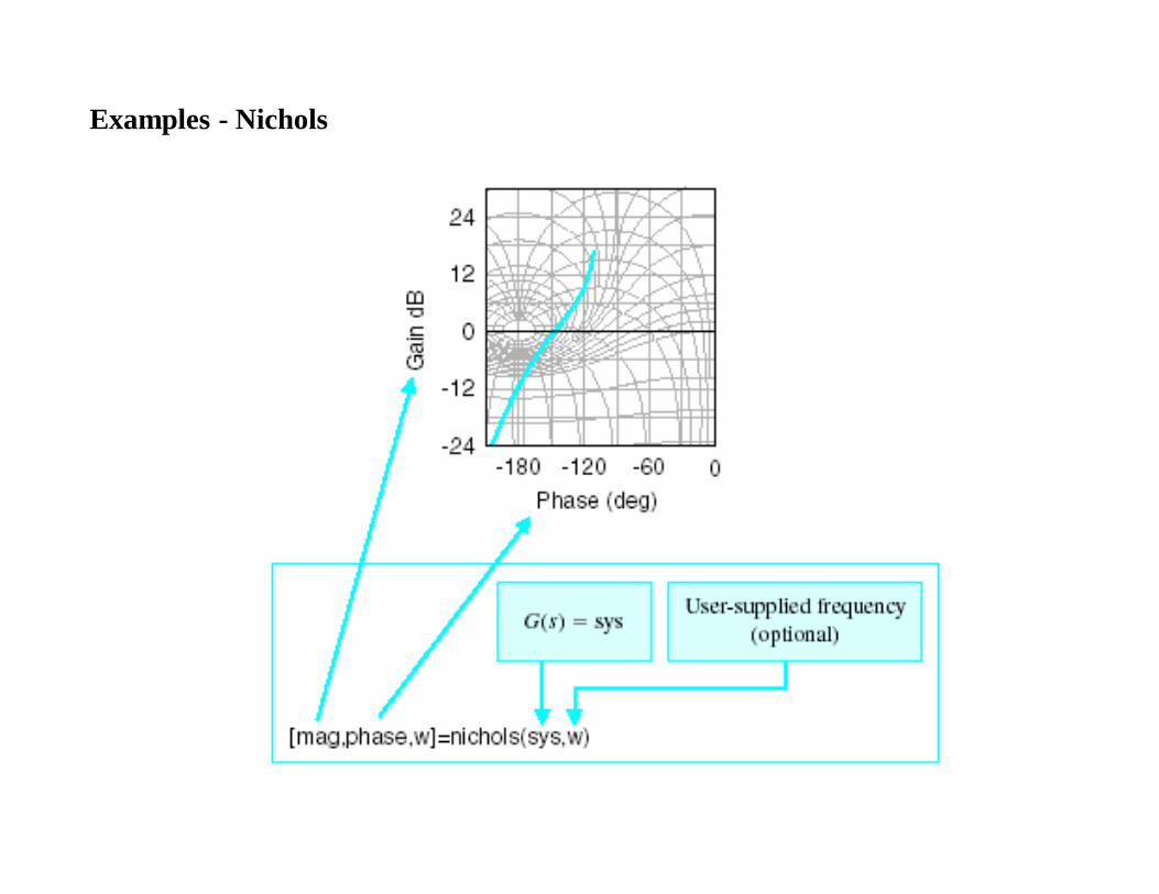
Examples - Nichols
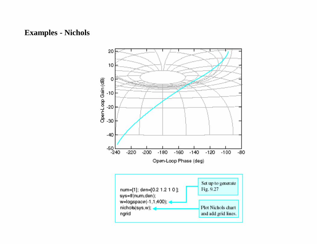
Examples - Nichols

UNIT - V
COMPENSATION TECHNIQUES
Lecture Outline
Introduction• A feedback control system that provides an optimum
performance without any necessary adjustment is rare.
• In building a control system, we know that propermodification of the plant dynamics may be a simple way tomeet the performance specifications.
• This, however, may not be possible in many practicalsituations because the plant may be fixed and notmodifiable.
• Then we must adjust parameters other than those in the fixedplant.
Introduction
• In previous lectures, we have discussed root locusmethod for loop gain adjustment.
• We have found that to achieve the desired systemresponse, it is possible to adjust the system parametersbut it is often not enough.
Introduction• It is then required to reconsider the structure of the
system and redesign the system.
• The design problems, therefore, become those ofimproving system performance by insertion of acompensator.
• Compensator: A compensator is an additionalcomponent or circuit that is inserted into a controlsystem to equalize or compensate for a deficientperformance.
Introduction
• Necessities of compensation• A system may be unsatisfactory in:
Stability.
Speed of response.
Steady-state error.
• Thus the design of a system is concerned with the alteration
of the frequency response or the root locus of the system in
order to obtain a suitable system performance.

Compensation via Root Locus• Performance measures in the time domain:
– Peak time;
– Overshoot;
– Settling time for a step input;
– Steady-state error for test inputs
• These performance specifications can be defined in terms ofthe desirable location of the poles and zeros of the closed-loop.
• Root locus method can be used to find a suitable compensatorGc(s) so that the resultant root locus results in the desiredclosed-loop root configuration.
Compensation via Root Locus• The design by the root-locus method is based on reshaping
the root locus of the system by adding poles and zeros tothe system’s open-loop transfer function and forcing theroot loci to pass through desired closed-loop poles in the splane.
• The characteristic of the root-locus design is its being basedon the assumption that the closed-loop system has a pair ofdominant closed-loop poles.
• This means that the effects of zeros and additional poles donot affect the response characteristics very much.
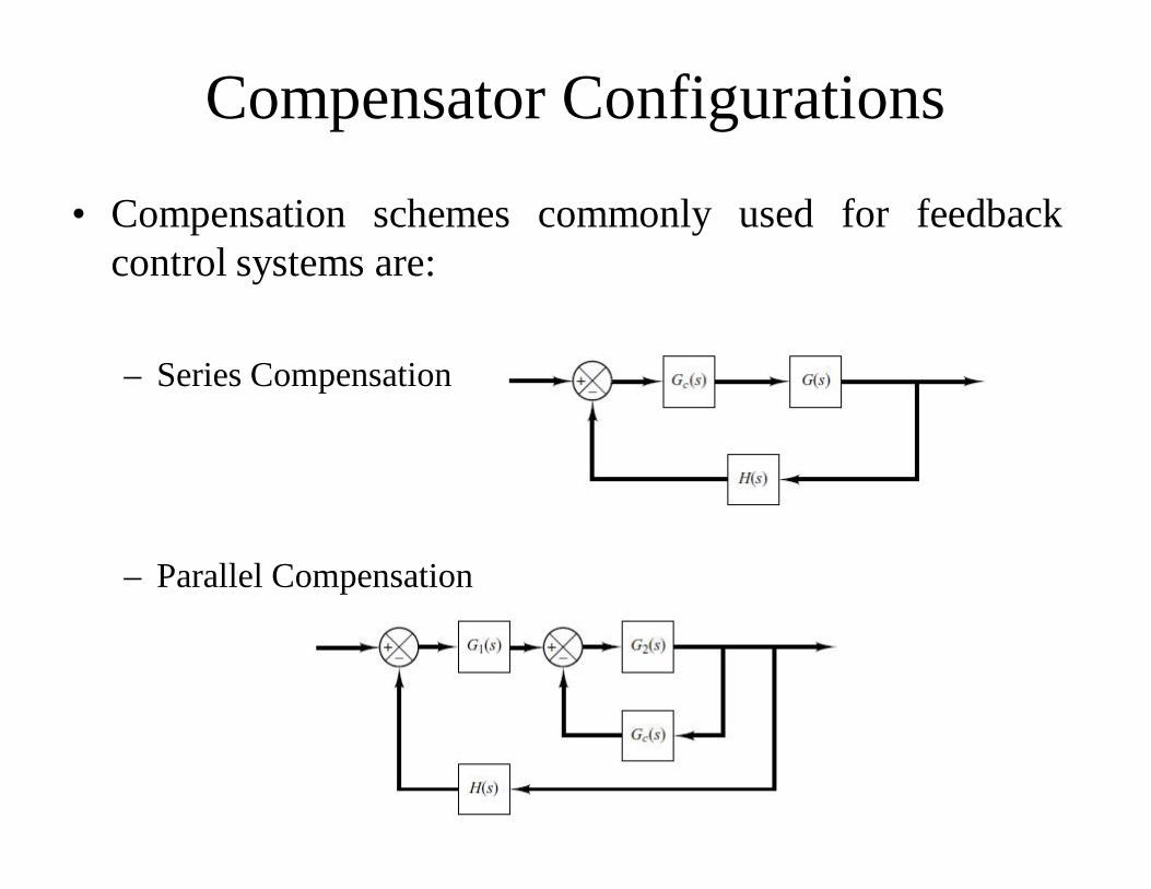
Compensator Configurations
• Compensation schemes commonly used for feedbackcontrol systems are:
– Series Compensation
– Parallel Compensation
Compensator Configurations
• The choice between series compensation and parallel
compensation depends on
– the nature of the signals
– the power levels at various points
– available components
– the designer’s experience
– economic considerations and so on.

Commonly Used Compensators
• Among the many kinds of compensators, widelyemployed compensators are the
– lead compensators
– lag compensators
– lag–lead compensators
Commonly Used Compensators
• Among the many kinds of compensators, widelyemployed compensators are the
– lead compensators• If a sinusoidal input is applied to the input of a network,
and the steady-state output (which is also sinusoidal)has a phase lead, then the network is called a leadnetwork.
Commonly Used Compensators
• Among the many kinds of compensators, widelyemployed compensators are the
– lag compensators• If the steady-state output has a phase lag, then the
network is called a lag network.
Commonly Used Compensators
• Among the many kinds of compensators, widelyemployed compensators are the
– lag–lead compensators• In a lag–lead network, both phase lag and phase lead
occur in the output but in different frequency regions.
• Phase lag occurs in the low-frequency region and phaselead occurs in the high-frequency region.

Commonly Used Compensators
• We will limit our discussions mostly to lead, lag, and lag–lead compensators realized by – Electronic devices such as circuits using operational
amplifiers
– Electrical Networks (RC networks)
– Mechanical Networks (Spring-Mass-Damper Networks).

Effect of Addition of Poles on Root Locus
• The addition of a pole to the open-loop transfer function has theeffect of pulling the root locus to the right, tending to lower thesystem’s relative stability and to slow down the settling of theresponse.

Effect of Addition of poles
Root Locus
Real Axis-1 -0.9 -0.8 -0.7 -0.6 -0.5 -0.4 -0.3 -0.2 -0.1 0
-0.5
-0.4
-0.3
-0.2
-0.1
0
0.1
0.2
0.3
0.4
0.5
1 0.8 0.6 0.4 0.2
0.985
0.94
0.86 0.76 0.64 0.5 0.34 0.16
0.985
0.94
0.86 0.76 0.64 0.5 0.34 0.16
SKSG )(
)1()(
SSKSGAdd a Pole at -1
Root Locus
Real Axis
Imag
Axi
s
-1.2 -1 -0.8 -0.6 -0.4 -0.2 0
-0.06
-0.04
-0.02
0
0.02
0.04
0.06
1.2 1 0.8 0.6 0.4 0.21
1
0.999
0.998 0.996 0.993 0.986 0.965 0.86
1
1
0.999
0.998 0.996 0.993 0.986 0.965 0.86
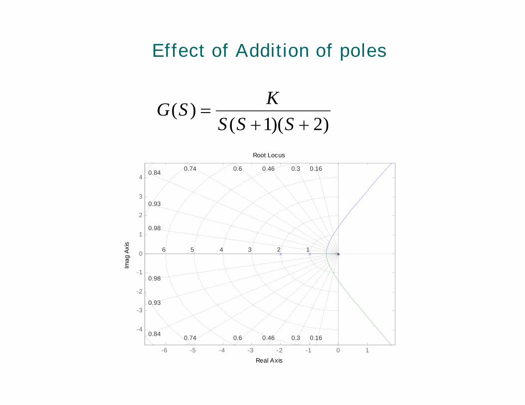
Effect of Addition of poles
)2)(1()(
SSSKSG
Root Locus
Real Axis
Imag
Axi
s
-6 -5 -4 -3 -2 -1 0 1
-4
-3
-2
-1
0
1
2
3
4
6 5 4 3 2 1
0.98
0.93
0.84 0.74 0.6 0.46 0.3 0.16
0.98
0.93
0.84 0.74 0.6 0.46 0.3 0.16

Effect of Addition of Zeros on Root Locus
• The addition of a zero to the open-loop transfer function hasthe effect of pulling the root locus to the left, tending to makethe system more stable and to speed up the settling of theresponse.
• Physically, the addition of a zero in the feed forward transferfunction means the addition of derivative control to thesystem.
• The effect of such control is to introduce a degree ofanticipation into the system and speed up the transientresponse.
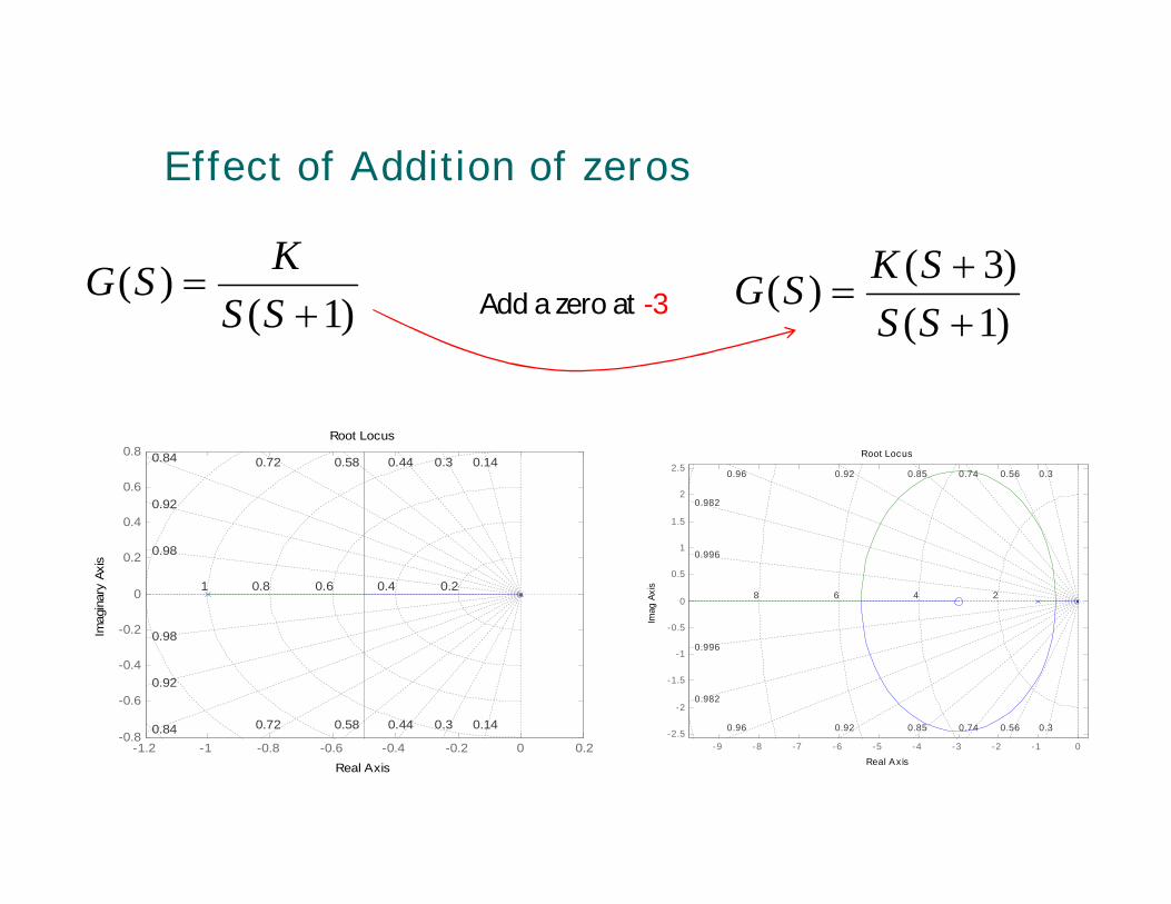
Effect of Addition of zeros
)1()(
SSKSG
)1()3()(
SSSKSGAdd a zero at -3
Root Locus
Real Axis
Imag
Axi
s
-9 -8 -7 -6 -5 -4 -3 -2 -1 0-2.5
-2
-1.5
-1
-0.5
0
0.5
1
1.5
2
2.5
8 6 4 2
0.996
0.982
0.96 0.92 0.85 0.74 0.56 0.3
0.996
0.982
0.96 0.92 0.85 0.74 0.56 0.3
-1.2 -1 -0.8 -0.6 -0.4 -0.2 0 0.2-0.8
-0.6
-0.4
-0.2
0
0.2
0.4
0.6
0.80.140.30.440.580.720.84
0.92
0.98
0.140.30.440.580.720.84
0.92
0.98
0.20.40.60.811.2
Root Locus
Real Axis
Imag
inar
y Ax
is
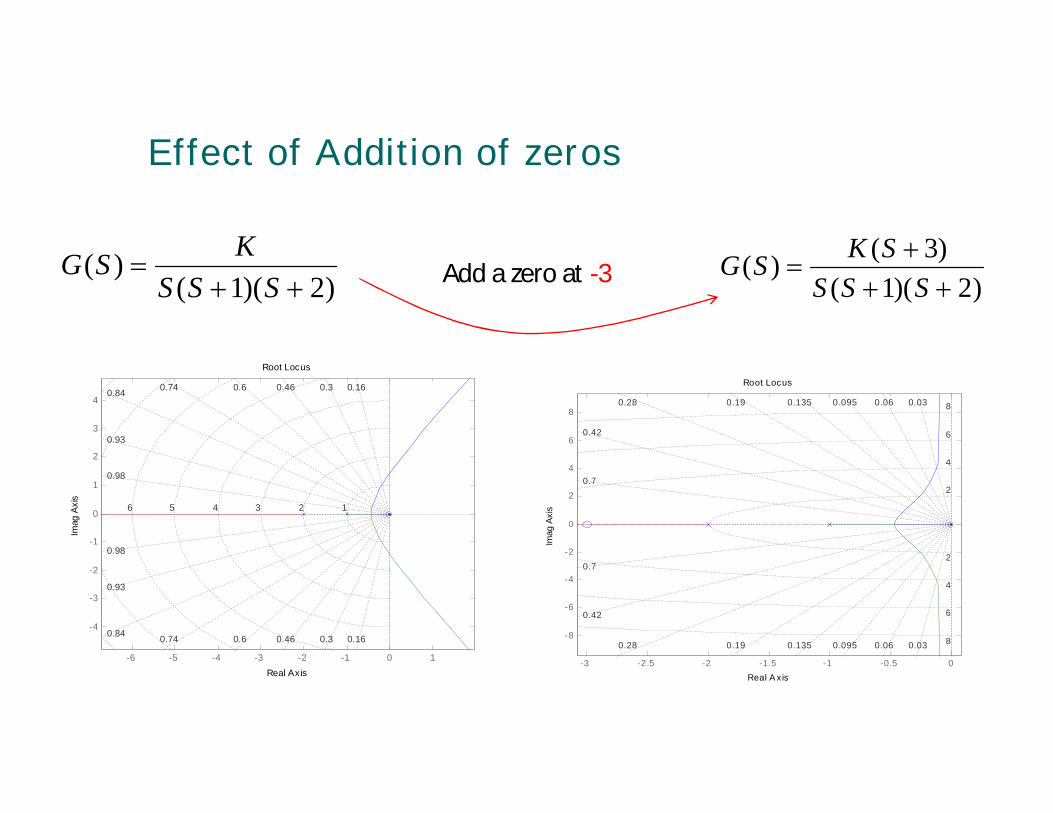
Effect of Addition of zeros
)2)(1()(
SSSKSG
Root Locus
Real Axis
Imag
Axi
s
-6 -5 -4 -3 -2 -1 0 1
-4
-3
-2
-1
0
1
2
3
4
6 5 4 3 2 1
0.98
0.93
0.84 0.74 0.6 0.46 0.3 0.16
0.98
0.93
0.84 0.74 0.6 0.46 0.3 0.16
)2)(1()3()(
SSSSKSG
Root Locus
Real A xis
Imag
Axi
s
-3 -2.5 -2 -1.5 -1 -0.5 0
-8
-6
-4
-2
0
2
4
6
8
8
6
4
2
8
6
4
2
0.7
0.42
0.28 0.19 0.135 0.095 0.06 0.03
0.7
0.42
0.28 0.19 0.135 0.095 0.06 0.03
Add a zero at -3