Control Systems Implementation Laboratory:

Control and Automation System Design Challenges

Kevin M. Passino and Nicanor QuijanoThe Ohio State University

Department of Electrical Engineering2015 Neil Avenue, Columbus Ohio, 43210

March 29, 2002

Abstract

This document lists a variety of control and automation system design challenges for the experimentsthat we have in our laboratory. Challenges are defined via a brief description of each plant and in somecases by providing a model of the plant. This document is not intended to be a complete compilation ofplant models and design challenges. Plant model development is discussed in more detail in literatureavailable in the lab for some of the experiments. The student should try to identify their own challengesthat they would like to address in the laboratory. Moreover, the students will naturally encounter manyspecific challenges as they attempt to implement control strategies.

Contents

1 Conventional Control Systems 21.1 Control System Design Challenges . . . . . . . . . . . . . . . . . . . . . . . . . . . . . . . . . 21.2 DC Servo . . . . . . . . . . . . . . . . . . . . . . . . . . . . . . . . . . . . . . . . . . . . . . . 31.3 Flexible Joint . . . . . . . . . . . . . . . . . . . . . . . . . . . . . . . . . . . . . . . . . . . . . 41.4 Flexible Link . . . . . . . . . . . . . . . . . . . . . . . . . . . . . . . . . . . . . . . . . . . . . 81.5 Ball and Beam . . . . . . . . . . . . . . . . . . . . . . . . . . . . . . . . . . . . . . . . . . . . 91.6 Inverted Pendulum . . . . . . . . . . . . . . . . . . . . . . . . . . . . . . . . . . . . . . . . . . 101.7 Water Tanks . . . . . . . . . . . . . . . . . . . . . . . . . . . . . . . . . . . . . . . . . . . . . 111.8 Cube . . . . . . . . . . . . . . . . . . . . . . . . . . . . . . . . . . . . . . . . . . . . . . . . . . 121.9 Helicopter . . . . . . . . . . . . . . . . . . . . . . . . . . . . . . . . . . . . . . . . . . . . . . . 13

2 Complex Hierarchical and Distributed Control Systems 132.1 Automation Design Challenges . . . . . . . . . . . . . . . . . . . . . . . . . . . . . . . . . . . 132.2 Building Temperature Control . . . . . . . . . . . . . . . . . . . . . . . . . . . . . . . . . . . . 152.3 Distributed Dynamic Resource Allocation for Balls in Tubes . . . . . . . . . . . . . . . . . . . 152.4 Cooperative Scheduling for Multi-Agent Fire Control . . . . . . . . . . . . . . . . . . . . . . . 162.5 Uniform Planar Hybrid Temperature Control . . . . . . . . . . . . . . . . . . . . . . . . . . . 162.6 Software Development Tools for Complex Control Systems . . . . . . . . . . . . . . . . . . . . 16

1

1 Conventional Control Systems

1.1 Control System Design Challenges

Here, we list some generic challenges encountered in control systems development, list some methods toovercome them, and then in the subsequent subsections outline the specific challenges for some of the plantsin our laboratory. Moreover, we briefly outline a list of different methods you may consider to apply to theplants in our laboratory.

Assuming you use feedback control, the design objectives (also called “closed-loop specifications” or“performance objectives”), i.e., what you want the control system to achieve, can involve many factors,including:

• Tracking.

• Reducing the effects of adverse conditions and uncertainty.

• Behavior in terms of time responses (e.g., stability, a certain rise-time, overshoot, and steady statetracking error).

• Engineering goals such as cost and reliability.

You can consider applying a wide array of control techniques to the plants in our laboratory. The popularmethods for control are the following:

• Proportional-integral-derivative (PID) control: Over 90% of the controllers in operation today are PIDcontrollers (or at least some form of PID controller like a P or PI controller). This approach is oftenviewed as simple, reliable, and easy to understand. Often, heuristics are used quite effectively to tunePID controllers (e.g., the Zeigler-Nichols tuning rules).

• Classical control: Lead-lag compensation, Bode and Nyquist methods, root-locus design, and so on.

• State-space methods: State feedback, observers, and so on.

• Optimal control: Linear quadratic regulator, use of Pontryagin’s minimum principle or dynamic pro-gramming, and so on.

• Robust control: H2 or H∞ methods, µ-synthesis, quantitative feedback theory, loop shaping, and soon.

• Nonlinear methods: Feedback linearization, Lyapunov redesign, sliding mode control, backstepping,and so on.

• Adaptive control: Model reference adaptive control, self-tuning regulators, nonlinear adaptive control,and so on.

• State and parameter estimation: Observers, Kalman filters, etc.

• Stochastic control: Minimum variance control, linear quadratic gaussian (LQG) control, stochasticadaptive control, and so on.

• Discrete event systems: Petri nets, automata, supervisory control, infinitesimal perturbation analysis,and so on.

• Hybrid systems: Control of systems that can most conveniently be represented by a combination ofcontinuous time differential equations and discrete event system models.

• Intelligent control: Neural networks, rule-based control (fuzzy, expert), planning systems, attentionalsystems, learning (adaptive) control, genetic algorithms for off-line design and on-line tuning, foragingmethods, game-theoretic approaches, general hierarhical and distributed intelligent control.

2

Most of these methods rely on the existence of “design models” and “truth models.” Hence, a challengethat is present for each of the plants in the laboratory is how to develop models, or improve on the ones thatwe already have. There are two basic approaches for model development: physics-based model developmentand system identification. A typical challenge is to try to develop a more accurate design model, but onethat is also useful for the systematic development of a controller. Another challenge is to develop a truthmodel and test its validity in simulation against the actual experiment.

1.2 DC Servo

The Quanser DC servo is shown in Figure 1. The input is the voltage Vin. There are three sensors. Thereare two different ones for shaft angle θ, a potentiometer and an encoder. There is also a tachometer formeasuring θ. This DC servo serves as the actuation for the flexible joint, flexible link, ball and beam, androtational inverted pendulum that are discussed below.

Figure 1: DC servo.

Suppose that you are concerned with position control. The transfer function for this case is

θ(s)Vin(s)

=1

s(sRmJeq

KmKg+ KmKg)

(1)

Here, Jeq = K2gJm + JI . The parameters values are Rm = 2.6 Ω ,Km = 0.00767 V/rad/sec, Kg = 14 : 1,

Jm = 3.87× 10−7 Kg.m2, and JI = 7.22× 10−6 Kg.m2 and this gives

θ(s)Vin(s)

=1

s(0.0020s + 0.1074)(2)

The root locus design for a unity feedback control system is given in Figure 2. From this figure, you can seethat a proportional controller can speed up the response, but if the gain is too high, then you can expectovershoot in response to a step reference input. How would a PD controller work? A PID? Note that

3

this plant can be damaged if you place high frequency oscillations into the DC servo in Vin (see Quanserdocumentation) and hence this is a concern for experiments (flexible link, flexible joint, ball and beam,pendulum). This must be carefully taken into consider in design and implementation. .

Root locus design for θ (s) / Vin

(s)

Real Axis

Imag

Axi

s

−40 −35 −30 −25 −20 −15 −10 −5 0

−10

−8

−6

−4

−2

0

2

4

6

8

10

Figure 2: Root locus for control system for DC servo

1.3 Flexible Joint

The flexible joint is shown in Figure 3. A mass can be added to the end point of the arm and there are9 different ways that springs can be attached, and there are three different types of springs each with adifferent spring constant. This allows for studying a variety of flexibility effects. There is an encoder formeasuring the angle of the link relative to the motor shaft angle, and of course the sensors from the DCservo can be used.

The purpose of the experiment is to design a controller which allows you to command a desired tip angleposition. For this experiment, we have the following variables:

• θ is the DC servo output shaft angle.

• Kstiff is a linear estimate of the joint stiffness, and is given by: Kstiff = δMδθ

|θ=0, where M is therestoring moment. There are three different springs that are included with the experiment, springs #1,#2, and #3. There are three possible springs each with different stiffness characteristics and severalanchor points on the flexible link (A, B, C for one end of the spring and 1, 2, and 3 for the other end).For the case where we use spring #2 at anchors [A, 3], we have that Kstiff = 1.6108 Nm/rad.

• α is the relative angle of the arm to the DC servo output shaft angle, i.e. it is the measurement of theangular deflection of the arm.

• The total inertia of the motor output is given by Jhub, and in this case is equal to 0.0021 Kgm2 .

• The total inertia of the arm is given as Jload , and in this case is equal to 0.0059 Kgm2 .

• R is the distance from the reference point of the joint to where you fix the spring in the anchor points.For the case described above, the distance is equal to 0.0762 m.

• Kg is the gear ratio, and for this case is equal to 14:1.

4

Figure 3: Flexible joint.

• Km is one of the motor torque constant, and for this case it is equal to 0.00767 V/rad/sec.

We have:

L = 0.0318; % m #1: 0.0254, #2: 0.0318 #3: defaultd = 0.0318; % m A: default; B: 0.0254; C: 0.0191r = 0.0318; % mJ_hub = 0.0021; % Kgm^2J_load = 0.0059; % #0: 0.0021; #1: 0.0042; #2: 0.0048; #3: default, Kgm^2R = 0.0762; % #1: 0.101; #2: 0.089; #3: default, mKm = 0.00767; % V/rad/secKgi = 14; % 14:1Kge = 5; % it could be also 5:1Fr = 1.33; % #1: 0.83; #2: 1.33; #3: 1.78, N (refers to a spring property)K = 368; % #1: 220; #2: 368; #3: 665, N/m (refers to a spring property)Rm = 2.6; % Ohms

D = r^2 + (R-d)^2;Kstiff = (2*R/D^(3/2))*((D*d-R*r^2)*Fr + (D^(3/2)*d - D*L*d + R*r^2*L)*K)Kg = Kgi*Kge;

A state space model for this plant

x = Ax + Bu (3)y = Cx

has u = Vin,

x =[θ, α, θ, α

]

5

A =

0 0 1 00 0 0 1

0 Kstiff

Jhub

−K2mK2

g

RJhub0

0 −Kstiff (Jload+Jhub)JhubJload

K2mK2

g

RJhub0

B =

00

KmKg

RJhub−KmKg

RJhub

With the above parameter values, Matlab gives:

A =

0 0 1.0000e+00 00 0 0 1.0000e+000 7.6705e+02 -5.2795e+01 00 -1.0401e+03 5.2795e+01 0

B =

00

9.8333e+01-9.8333e+01

C =

1 0 0 00 1 0 01 1 0 0

eigenvalues =

0-8.9913e+00 + 1.8254e+01i-8.9913e+00 - 1.8254e+01i-3.4813e+01

Transfer function:-4.974e-14 s^3 + 98.33 s^2 - 7.458e-11 s + 2.685e04---------------------------------------------------

s^4 + 52.8 s^3 + 1040 s^2 + 1.441e04 s

zeros =

1.9770e+153.1017e-13 + 1.6523e+01i3.1017e-13 - 1.6523e+01i

6

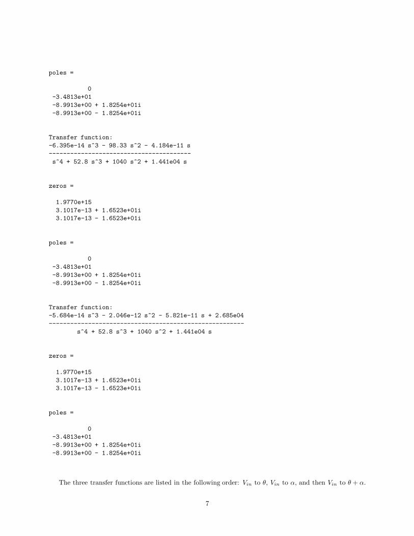
poles =

0-3.4813e+01-8.9913e+00 + 1.8254e+01i-8.9913e+00 - 1.8254e+01i

Transfer function:-6.395e-14 s^3 - 98.33 s^2 - 4.184e-11 s----------------------------------------s^4 + 52.8 s^3 + 1040 s^2 + 1.441e04 s

zeros =

1.9770e+153.1017e-13 + 1.6523e+01i3.1017e-13 - 1.6523e+01i

poles =

0-3.4813e+01-8.9913e+00 + 1.8254e+01i-8.9913e+00 - 1.8254e+01i

Transfer function:-5.684e-14 s^3 - 2.046e-12 s^2 - 5.821e-11 s + 2.685e04-------------------------------------------------------

s^4 + 52.8 s^3 + 1040 s^2 + 1.441e04 s

zeros =

1.9770e+153.1017e-13 + 1.6523e+01i3.1017e-13 - 1.6523e+01i

poles =

0-3.4813e+01-8.9913e+00 + 1.8254e+01i-8.9913e+00 - 1.8254e+01i

The three transfer functions are listed in the following order: Vin to θ, Vin to α, and then Vin to θ + α.

7

Notice that several terms in the numerators are essentially zero compared to the size of the other terms sothat some of the zero locations are essentially at infinity as you would expect.

The objective is to regulate α to zero while moving the endpoint position to a specific angle. What typeof compensation would be effective for this plant? What should the closed-loop specifications be? Can youmeasure the entire state and hence use state feedback control? Can you, via the use of state estimation, useonly a subset of the available measurements and still come up with an effective control strategy? Can youderive a nonlinear model? Could you derive one of a form that is both accurate and of a form that is usefulfor some nonlinear controller design method (e.g., backstepping or feedback linearization)? What types ofdisturbances would you typically encounter for this plant? What if there is a weight change at the linkendpoint? What if you change the configuration of the springs or the spring type to change the flexibilityeffects? How could you model this? Would an adaptive or robust control approach be useful to be able toconstruct a controller that could cope with a wide range of different endpoint masses and flexibility effects?

1.4 Flexible Link

The flexible link is show in Figure 4. As with the flexible joint the objective is fast endpoint position control.There is a strain gage sensor that is calibrated to provide one volt output for every inch of deflection at thetip, and of course the sensors from the DC servo can be used.

Figure 4: Flexible link.

This experiment is similar to the flexible joint experiment except that the link is flexible rather than thejoint. The state space model has u = Vin, x = [θ, α, θ, α], and y = θ + α with

A =

0 0 1 00 0 0 10 2165 −53.6 00 −2797 53.6 0

B =

0099−99

andC =

[1 1 0 0

]

8

The entire state, except for α can be measured and α can typically be estimated in software via a filteredderivative calculation.

In this case, since the matrix C is defined as above, the output will be the total deflection of the tip.Using these matrices, and the command ss2tf in Matlab, we obtain the transfer function

G4(s) =−7.816× 10−14s3 − 6.366× 10−12s2 − 8.731× 10−11s + 6.257× 104

s4 + 53.6s3 + 2797s2 + 33875s(4)

Notice that the first three terms in the numerator are essentially zero compared to the constant term in thenumerator. The poles and zeros are:

• Poles:

1. 0

2. −15.3251

3. −19.1374 + 42.9440i

4. −19.1374− 42.9440i

• Zeros (as expected the zeros are essentially at ∞):

1. −4.6429× 105 + 8.0412× 105i

2. −4.6429× 105 − 8.0412× 105i

3. 9.2849× 105

The root locus plot for a unity feedback control system is shown in Figure 5. What type of compensationwould be effective for this plant? What should the closed-loop specifications be? Can you measure the entirestate and hence use state feedback control? Can you, via the use of state estimation, use only a subset ofthe available measurements and still come up with an effective control strategy? Can you derive a nonlinearmodel? Could you derive one of a form that is both accurate and of a form that is useful for some nonlinearcontroller design method (e.g., backstepping or feedback linearization)? What types of disturbances wouldyou typically encounter for this plant? What if there is a weight change at the link endpoint? How couldyou model this? Would an adaptive or robust control approach be useful to be able to construct a controllerthat could cope with a wide range of different endpoint masses?

1.5 Ball and Beam

The ball and beam experiment is shown in Figure 6. There is a sensor for ball position, and of course thesensors from the DC servo can be used. The objective is to balance the ball at a desired location.

For the ball and beam experiment we have the distance x, the radius of the output gear r, gravity g, theangle of the beam α, the length of the beam L, and the angle of the DC servo as θ. With these variables,

X(s)θ(s)

=−5rg

7Ls2(5)

so that the dynamics can be approximated as a double integrator. The parameter values are g = 9.8 m/s2,L = 43.18 cm, and r = 2.54 cm.

The root locus for a unity feedback cases covers the jω axis. Based on this root locus what type ofcompensation would you expect to be effective? A PD controller? What should the closed-loop specificationsbe? What is the state? What is the state space model? Can you measure the entire state and hence usestate feedback control? Can you derive a nonlinear model? Could you derive one of a form that is bothaccurate and of a form that is useful for some nonlinear controller design method (e.g., backstepping orfeedback linearization)? What types of disturbances would you typically encounter for this plant? What ifthere is a weight change at one end of the beam? How could you model this? Would an adaptive or robustcontrol approach be useful to be able to construct a controller that could cope with a wide range of differentsuch masses?

9

Root locus plot for the flexible link

Real Axis

Imag

Axi

s

−150 −100 −50 0 50 100

−150

−100

−50

0

50

100

150

Figure 5: Root locus for Equation (4).

Figure 6: Ball and beam.

1.6 Inverted Pendulum

The rotational inverted pendulum is shown in Figure 7. There is a sensor for measuring the pendulumangle, and of course the sensors from the DC servo can be used. The inverted pendulum is a classical verywell-studied and simple nonlinear control experiment.

The model for our inverted pendulum has

x = [θ, αu, θ, αu]

Where θ is the angle made by the base and αu is the angle made by the pendulum relative to the vertical.Sensors are provided for all the state elements except for αu (but perhaps you can use software to estimateit and θ so that you do not need the tachometer for it). The state space model can be derived using physicsand data sheets provide the parameters.

There are several types of control problems that can be considered:

1. Swing-up: Design a controller that will “destabilize” the equilibrium corresponding to the pendulumhanging down.

10

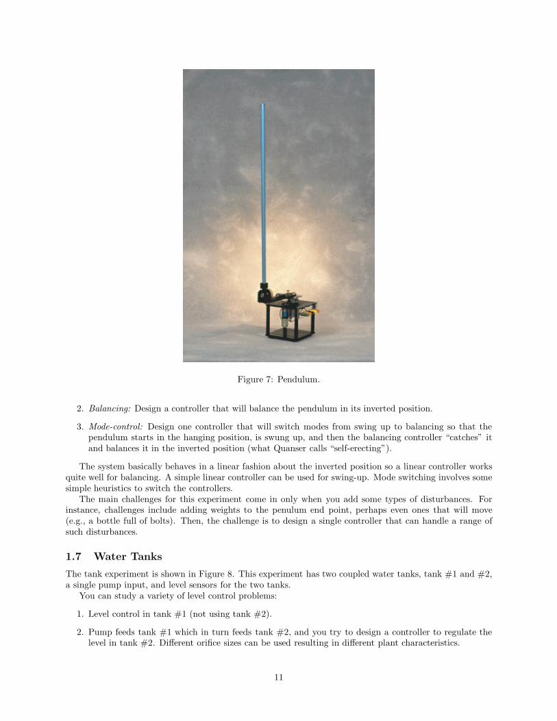
Figure 7: Pendulum.

2. Balancing: Design a controller that will balance the pendulum in its inverted position.

3. Mode-control: Design one controller that will switch modes from swing up to balancing so that thependulum starts in the hanging position, is swung up, and then the balancing controller “catches” itand balances it in the inverted position (what Quanser calls “self-erecting”).

The system basically behaves in a linear fashion about the inverted position so a linear controller worksquite well for balancing. A simple linear controller can be used for swing-up. Mode switching involves somesimple heuristics to switch the controllers.

The main challenges for this experiment come in only when you add some types of disturbances. Forinstance, challenges include adding weights to the penulum end point, perhaps even ones that will move(e.g., a bottle full of bolts). Then, the challenge is to design a single controller that can handle a range ofsuch disturbances.

1.7 Water Tanks

The tank experiment is shown in Figure 8. This experiment has two coupled water tanks, tank #1 and #2,a single pump input, and level sensors for the two tanks.

You can study a variety of level control problems:

1. Level control in tank #1 (not using tank #2).

2. Pump feeds tank #1 which in turn feeds tank #2, and you try to design a controller to regulate thelevel in tank #2. Different orifice sizes can be used resulting in different plant characteristics.

11

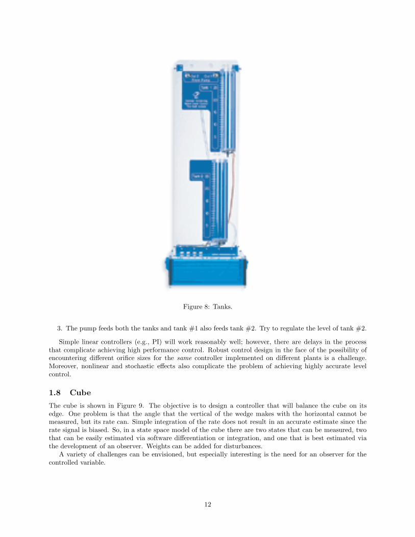
Figure 8: Tanks.

3. The pump feeds both the tanks and tank #1 also feeds tank #2. Try to regulate the level of tank #2.

Simple linear controllers (e.g., PI) will work reasonably well; however, there are delays in the processthat complicate achieving high performance control. Robust control design in the face of the possibility ofencountering different orifice sizes for the same controller implemented on different plants is a challenge.Moreover, nonlinear and stochastic effects also complicate the problem of achieving highly accurate levelcontrol.

1.8 Cube

The cube is shown in Figure 9. The objective is to design a controller that will balance the cube on itsedge. One problem is that the angle that the vertical of the wedge makes with the horizontal cannot bemeasured, but its rate can. Simple integration of the rate does not result in an accurate estimate since therate signal is biased. So, in a state space model of the cube there are two states that can be measured, twothat can be easily estimated via software differentiation or integration, and one that is best estimated viathe development of an observer. Weights can be added for disturbances.

A variety of challenges can be envisioned, but especially interesting is the need for an observer for thecontrolled variable.

12

Figure 9: Cube.

1.9 Helicopter

The helicopter “model” is mounted on a fixed base and the two propellers are driven by two DC motors (twoplant inputs) that control pitch and yaw as shown in Figure 10. There are measurements of the pitch andyaw via encoders. The objective is to design a controller that can allows you to command a desired pitchand yaw. Also, you can study the performance of the system with a human in the loop via the use of a joystick.

This is a multi-input multi-output (MIMO) control system design problem that is coupled due to pitch-yaw coupling. Disturbances can be added via weights.

2 Complex Hierarchical and Distributed Control Systems

In this section we overview the plants that we have in the laboratory for the study of hierarchical anddistributed control. Our motivation for including such problems is the presence of a wide variety of complexhierarchical and distributed control systems operating in industry. For example, there are commercialdistributed control systems (DCS) that are typically composed of a network of sequencing logic and PIDalgorithms and are used for process control and manufacturing systems.

While a student may gain some experience with such control systems while in industry, it is typicallynot possible to have full-scale versions of such control systems available at a university due to cost con-straints. Yet, it seems likely that the demands of industrial automation will press the universities to provideeducational experiences in this area (e.g., research on principles and theory of complex control systems andlaboratory experience with such systems). This provides the prime motivation for including a set of plantsand control system design challenges for complex hierarchical and distributed control systems.

2.1 Automation Design Challenges

There are many application-specific challenges you will encounter in trying to implement a control system(e.g., interfacing issues with the plant and operator), and these can be particularly numerous and difficultfor hierarchical distributed control systems. Here we try to provide a brief overview of some typical designchallenges. First, it is important to keep in mind that all the control system design problems that we outlinedin the last section are also encountered here (e.g., modeling, robustness, disturbance rejection, performance

13

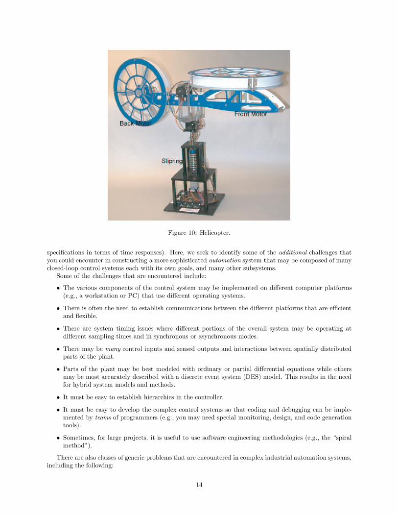
Figure 10: Helicopter.

specifications in terms of time responses). Here, we seek to identify some of the additional challenges thatyou could encounter in constructing a more sophisticated automation system that may be composed of manyclosed-loop control systems each with its own goals, and many other subsystems.

Some of the challenges that are encountered include:

• The various components of the control system may be implemented on different computer platforms(e.g., a workstation or PC) that use different operating systems.

• There is often the need to establish communications between the different platforms that are efficientand flexible.

• There are system timing issues where different portions of the overall system may be operating atdifferent sampling times and in synchronous or asynchronous modes.

• There may be many control inputs and sensed outputs and interactions between spatially distributedparts of the plant.

• Parts of the plant may be best modeled with ordinary or partial differential equations while othersmay be most accurately described with a discrete event system (DES) model. This results in the needfor hybrid system models and methods.

• It must be easy to establish hierarchies in the controller.

• It must be easy to develop the complex control systems so that coding and debugging can be imple-mented by teams of programmers (e.g., you may need special monitoring, design, and code generationtools).

• Sometimes, for large projects, it is useful to use software engineering methodologies (e.g., the “spiralmethod”).

There are also classes of generic problems that are encountered in complex industrial automation systems,including the following:

14

1. Sequencing and scheduling: There are typically problems that demand the sequencing of operations(e.g., in a manufacturing system) and often the plant is best modeled by a finite state machine, Petrinet, some other DES model, or even a hybrid system model. There is a need for closed-loop schedulingfor dynamical systems that is robust and can be implemented in real-time.

2. Resource allocation: In many applications you must control what gets certain resources and at whichtimes they get them. Sometimes such “resources” can be split, and other times they may not be. Forinstance, in flexible manufacting systems there is the problem of controlling (scheduling) which partsa machine (a resource) should process (the control problem is to measure queues of incoming partsand decide which queue to service). In the “gas lift optimization” problem in an oil field you have toallocate natural gas to different oil wells to maximize the overall production rate.

3. Process-wide optimization: An important problem is how to optimize decisions taken across the entireprocess from inventory control to the end product to ensure minimization of cost of production, yetthe highest quality product.

4. Hierarchical and distributed control: As discussed above hierarchical and distributed control is oftenused in industry. It arises due to the need to “divide and conquer” large complex automation problems.

5. Hybrid control: There is often a need for hybrid combinations of linear, nonlinear, and discrete eventtype controllers that may operate synchronously or in an asychronous fashion.

It should be clear that there is no way that you can be expected to develop a full complex hierarchicaland distributed control system. You can, however, address some of these fundamental challenges via theexperiments that are described next since they have been constructed specifically to address typically-encountered “generic” challenges.

2.2 Building Temperature Control

The building temperature control experiment is shown in Figure 11. There are 8 rooms, each of which has atemperature sensor and heater (control input). Also, there are 4 fans that can be proportionally controlled(but which blow air only in one direction). The building has two floors which can be easily separated forstudy in isolation. Each floor has one wall that is easily removable for the study of different floor plans.There are many windows and doors, each of which can be manually opened or shut (e.g., to study theinteractions between the rooms when a door is left open, or when a window is open and there is then anambient temperature effect). Moreover, the fans can be placed in any window or door to move air in or outof a room. Also, it is easy to add more fans so that more plant inputs can be added (e.g., one coupling thetwo floors).

The plant currently has 8+4 = 12 control inputs and 8 temperature sensor outputs and hence is a MIMOcontrol problem. There are a wide variety of ways to induce disturbances. It is easy to study multi-zone andhierarchical distributed temperature control.

2.3 Distributed Dynamic Resource Allocation for Balls in Tubes

In this experiment there are two sets of four tubes each of which holds a ball that is levitated via sensingits height with an ultrasonic sensor and actuation via a proportionally controlled fan. One control objectivecould be to blow air so as to maximize the height of the balls in the tubes (i.e., to keep them levitated at amaximum height). The problem is that there is a manifold at the bottom of each set of tubes that couplesthem so that air must be allocated by the fans to the different tubes to maximize ball height (maximizing theheight of only one ball will result in lowering the height of several other balls). Also, there is an electricallycontrollable disturbance on the manifold, and the two manifolds can be coupled to study cross-couplingeffects between all eight tubes.

The experiment is only partially implemented as of the writing of this document (Spring’02). This quarterthe challenge for this experiment is to finish the construction of the experiment, get the individual controllersoperating for ball height regulation for the 8 tubes, and then design and test dynamic resource allocationstrategies for the entire set of tubes.

15

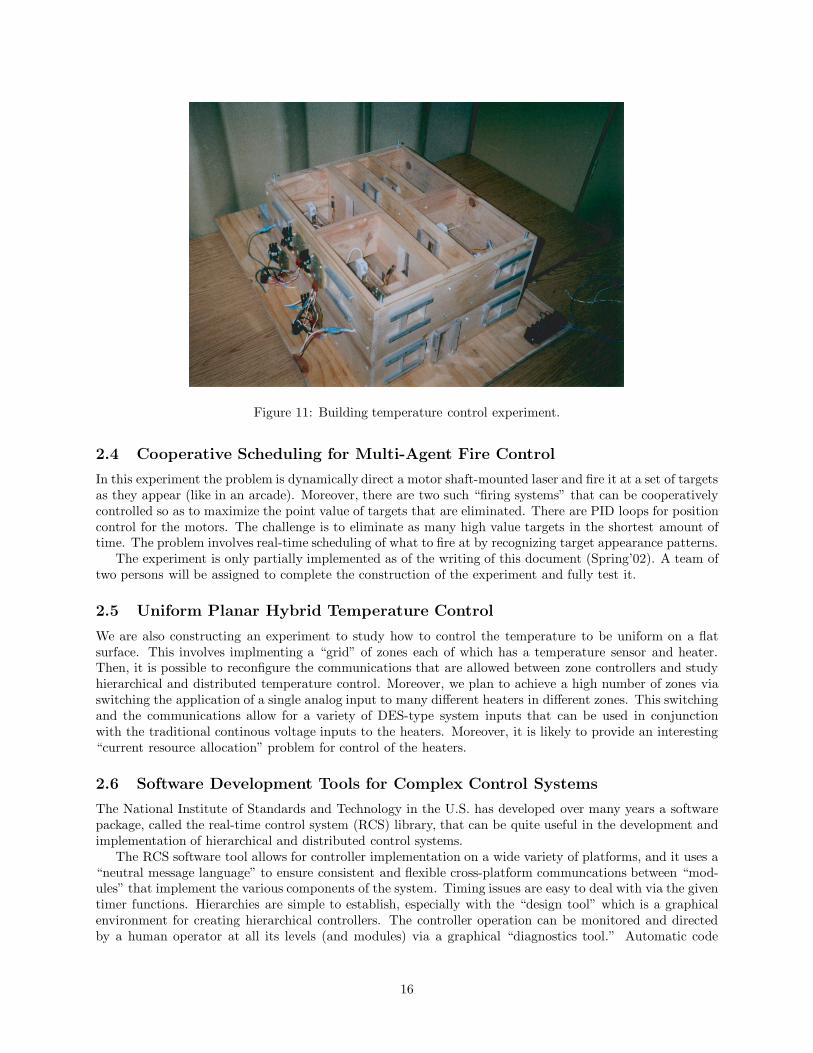
Figure 11: Building temperature control experiment.

2.4 Cooperative Scheduling for Multi-Agent Fire Control

In this experiment the problem is dynamically direct a motor shaft-mounted laser and fire it at a set of targetsas they appear (like in an arcade). Moreover, there are two such “firing systems” that can be cooperativelycontrolled so as to maximize the point value of targets that are eliminated. There are PID loops for positioncontrol for the motors. The challenge is to eliminate as many high value targets in the shortest amount oftime. The problem involves real-time scheduling of what to fire at by recognizing target appearance patterns.

The experiment is only partially implemented as of the writing of this document (Spring’02). A team oftwo persons will be assigned to complete the construction of the experiment and fully test it.

2.5 Uniform Planar Hybrid Temperature Control

We are also constructing an experiment to study how to control the temperature to be uniform on a flatsurface. This involves implmenting a “grid” of zones each of which has a temperature sensor and heater.Then, it is possible to reconfigure the communications that are allowed between zone controllers and studyhierarchical and distributed temperature control. Moreover, we plan to achieve a high number of zones viaswitching the application of a single analog input to many different heaters in different zones. This switchingand the communications allow for a variety of DES-type system inputs that can be used in conjunctionwith the traditional continous voltage inputs to the heaters. Moreover, it is likely to provide an interesting“current resource allocation” problem for control of the heaters.

2.6 Software Development Tools for Complex Control Systems

The National Institute of Standards and Technology in the U.S. has developed over many years a softwarepackage, called the real-time control system (RCS) library, that can be quite useful in the development andimplementation of hierarchical and distributed control systems.

The RCS software tool allows for controller implementation on a wide variety of platforms, and it uses a“neutral message language” to ensure consistent and flexible cross-platform communcations between “mod-ules” that implement the various components of the system. Timing issues are easy to deal with via the giventimer functions. Hierarchies are simple to establish, especially with the “design tool” which is a graphicalenvironment for creating hierarchical controllers. The controller operation can be monitored and directedby a human operator at all its levels (and modules) via a graphical “diagnostics tool.” Automatic code

16

generation is provided and tools are available to facilitate team-based development of a complex controller.It is interesting to note that RCS is a free software package that can be used to solve many of the problems

listed above, and is well-developed enough to use in practical industrial control and automation problems.A book covering all the details is:

V. Gazi, M. Moore, K. Passino, W. Shackleford, F. Proctor, and J. Albus, The RCS Handbook:Tools for Real Time Control Systems Software Development, John Wiley and Sons, Pub., NY,2000.

17