controller design by pole placement - fac.ksu.edu.sa · the calculated gains will be a good...

Controller Design by Pole placement

1. Introduction to control

2. Design of two position controller

3. Control design by pole placement

4. Control design by PID control

Dr Nassim Ammour CEN455 King Saud University 1

2

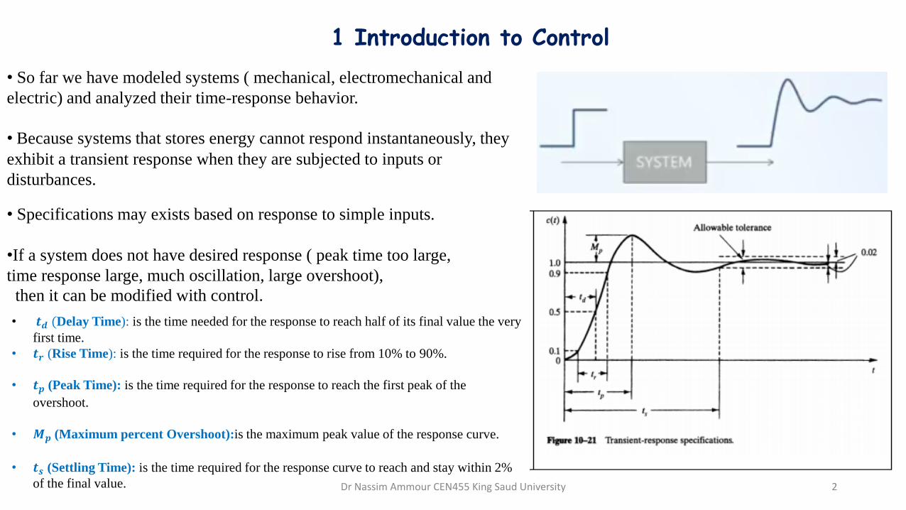
1 Introduction to Control

• So far we have modeled systems ( mechanical, electromechanical and

electric) and analyzed their time-response behavior.

• Because systems that stores energy cannot respond instantaneously, they

exhibit a transient response when they are subjected to inputs or

disturbances.

• Specifications may exists based on response to simple inputs.

•If a system does not have desired response ( peak time too large,

time response large, much oscillation, large overshoot),

then it can be modified with control.

• 𝒕𝒅 (Delay Time): is the time needed for the response to reach half of its final value the very

first time.

• 𝒕𝒓 (Rise Time): is the time required for the response to rise from 10% to 90%.

• 𝒕𝒑 (Peak Time): is the time required for the response to reach the first peak of the

overshoot.

• 𝑴𝒑 (Maximum percent Overshoot):is the maximum peak value of the response curve.

• 𝒕𝒔 (Settling Time): is the time required for the response curve to reach and stay within 2%

of the final value. Dr Nassim Ammour CEN455 King Saud University

3

1.1 Control architecture (feed-forward control)

- Simple to design (plant inversion).

• Open-loop control (feed-forward control).

U(s) = C(s) R(s).

If we ignore D(s)

Y(s) = P(s) C(s) R(s) .

To have Y(s) = R(s) we need to put P(s) C(s) =1

Therefore, C(s) = 1/P(s) (Design a controller = inverse of the plant)

-This is very simple and cheap (no feedback so no sensor needed, no software to interact with sensor, no signal processing

to use with the sensor).

-Not robust. (model error -> bad controller C(s)= 1/P(s) is not robust, disturbances change the plant , U(s) is not the only input)

- one way to address this limitations is to add feed-back.

Dr Nassim Ammour CEN455 King Saud University

4

1.3 Control architecture (feed-back control)

• Closed-loop control (feed-back control).

-More robust:

by measuring the output we can see the

fact of no convergence of the output to the input (due

to bad modeling or disturbances), and the controller

changes the control signal to improve the system behavior.

-More complicated and expensive:

Add sensors and hardware or software to process the sensors’ signals

- Can cause a stable system to become unstable.

For a stable system (poles in LHP) and stable controller (poles in LHP) but when we close the loop we obtain an unstable system .

-The response can be slower.

With feedback control we have to wait for the error to develop (dynamic of the plant) before establishing the control signal.


1.4 Control requirements

• Approach to Control design: Translate engineering specifications into control requirements, then design a controller to

meet those specifications.

1. Determine what the system should do and how to do it (design specification),

2. Determine the controller or compensator configuration relative to how it is connected to the controlled process.

3. Determine the parameter values of the controller to achieve the design goals.

• Example: example in cars, increases the comfort and safety of driving a car or reduces the fuel consumption and exhaust gas

emissions.

• Examples transient specifications (system step response): Time constant𝜏 (speed of response of a first order

system), over shoot 𝑀𝑝 , peak time 𝑡𝑝 , settle time 𝑡𝑠 and rise time 𝑡𝑟. (feasible analytically only for second-order systems, or

systems that can be approximated by a second-order system).

• Example steady-state specifications: Typically it is required that steady-state error be less than some amount, for

example ess <0.02. We can use the final value theorem for different types of reference inputs ess = 𝑙𝑖𝑚𝑠→0𝑠𝐸(𝑠)

Fig.1 controlled process

• Experiences and knowledge in physics, mathematics, and control theory are

required to design a stable controller with good performance.


6

2 On-Off (Two-position) Controller

• This is a nonlinear controller which is very simple and it does not need any design. The On-Off Controller is defined as:

𝑢 𝑡 = 𝑈𝑚𝑎𝑥 𝑖𝑓 𝑒 𝑡 > 0

𝑈𝑚𝑖𝑛 𝑖𝑓 𝑒 𝑡 < 0

Where : 𝑒 𝑡 = 𝑟 𝑡 − 𝑦 𝑡 is the tracking error and u(t) is the applied control system.

• Control signal u(t) can have only two possible values. (fully-on, High u(t) =Umax or fully-off, low u(t) =Umin) depending if error

is positive or negative. The main idea in this way of control, which only two control levels achieve desired value of the

controlled variable in shortest time possible.

• The control signal will oscillate between two levels (high frequency, damage the actuators) and good tracking accuracy is

achieved.

• The control signal never reach the zero value which means the process consumes energy (cost is high).

• To avoid this high frequency oscillation an hysteresis is introduced.

𝑢 𝑡 = 𝑈𝑚𝑎𝑥 𝑖𝑓 𝑒 𝑡 > +𝜀

𝑈𝑚𝑖𝑛 𝑖𝑓 𝑒 𝑡 < −𝜀


7

• The typical behavior of ON-OFF controller system is shown in Fig.1.

• Advantages: very simple, robust, and inexpensive.

• Drawbacks: large overshoot and undershoot.

• An on-off controller is the simplest form of temperature control device.

• On-off control is usually used where a precise control is not necessary

Fig.1 ON-OFF controller behavior

2.1 Advantages and Drawbacks of ON-OFF controller


0 0.1 0.2 0.3 0.4 0.5 0.6 0.7 0.8 0.9 1

-6

-4

-2

0

2

4

6

Time (sec)

0 0.1 0.2 0.3 0.4 0.5 0.6 0.7 0.8 0.9 10

0.2

0.4

0.6

0.8

1

1.2

1.4

Time (sec)

8

2.2 Example 1Control the water level system by two-position controller. The transfer function

of the water level system is: ℎ = 𝑢(𝑡)where h(t) is the water level system.

SOLUTION

• Simulation using: SIMULINK : With eps=0.1 and Umax=5 and Umin=-5,

• We got the following simulation results:

Fig.3 control signal

Fig.2 Output signal

Fig.1 Simulink Program


9

2.3 Example 2• For another case (ref=8v; =±1; On=5v and Off=-5v).

We have: 𝑢 = 5𝑣 when 𝑒 𝑡 ≻ −1; 𝑦𝑟𝑒𝑓 − 𝑦 𝑡 ≻ −1 𝑜𝑟 𝑦 𝑡 < 𝑦𝑟𝑒𝑓 + 1 = 9

Or 𝑢 = −5𝑣 when 𝑒 𝑡 < 1; 𝑦𝑟𝑒𝑓 − 𝑦 𝑡 < 1 𝑜𝑟 𝑦 𝑡 > 𝑦𝑟𝑒𝑓 − 1 = 7

The problem is when 7 < 𝑦 𝑡 < 9, the control signal keeps the previous value.

• We need to design a controller with smooth control signal, less energy

consuming, and good tracking performances.

0 0.5 1 1.5 2 2.5 3 3.5 4-5

0

5

10

Time (s)

Output

Control Signal

Fig.1 output signal and control signal

Y(t) > 𝑦𝑟𝑒𝑓 − 𝜀

Y(t) < 𝑦𝑟𝑒𝑓 + 𝜀


3 Design by pole placement• Poles of a system affect the time response. Pole

Delay Time: 𝑇𝑑 =1+0.7 𝜉

𝜔𝑛Rise Time: 𝑇𝑟 =

𝜋−𝛽

𝜔𝑑

Peak Time: 𝑇𝑝 =𝜋

𝜔𝑑=

𝜋

𝜔𝑛 1−𝜉2 Maximum Overshoot: 𝑀𝑝 = 𝑒

− 𝜋 𝜉

1−𝜉2× 100%

Settling Time: 𝑇𝑠 =4

𝜉 𝜔𝑛

2nd order system transfer function: 𝐺(𝑠) =𝜔𝑛

2

𝑠2+2𝜉 𝜔𝑛+𝜔𝑛2

𝜔𝑛 is the Natural frequency

𝜉 is Damping Ratio

The poles of the system: 𝑃1,2 = 𝜎 ± 𝑗𝜔𝑑 = −𝜉𝜔𝑛 ± 𝑗𝜔𝑛 1 − 𝜉2

Controller Design

• Choose controller gains (for ex: 𝐾𝑝, 𝐾𝐼, and 𝐾𝐷) so that poles of the close-loop system meet given requirements.

• If the system is simple ( canonical first order system or canonical second order system) can employ algebra (precise

relationships between poles and the shape of the step response).

• If the system is non-canonical (higher order system) the relationships is not exact. One idea is to place one or two dominant

poles to meet our requirements and place the rest of poles to be significantly faster, so that we can one sense neglect the effect of

the dynamics for the other transient response. Dr Nassim Ammour CEN455 King Saud University 10

3.1 Example

• Find the close-loop transfer function for a cruise control system with PI controller (How to design a PI controller, in other words how to choose the gains proportional gain 𝐾𝑝 and integral gain 𝐾𝐼 for a first order system).

• First step in the design is to find the close-loop transfer function to see the effect of the controller gains on the close-loop poles.

𝑉(𝑠)

𝑉𝑑𝑒𝑠(𝑠)=

𝑓𝑜𝑟𝑤𝑎𝑟𝑑

1 + 𝑙𝑜𝑜𝑝=

(𝐾𝑝 + 𝐾𝐼1𝑠)(

1𝑚𝑠 + 𝑏

)

1 + (𝐾𝑝 + 𝐾𝐼1𝑠)(

1𝑚𝑠 + 𝑏

)=

𝐾𝑝 𝑠 + 𝐾𝐼

𝑠 𝑚𝑠 + 𝑏 + 𝐾𝑝 𝑠 + 𝐾𝐼=


𝑚 𝑠2 + 𝑏 + 𝐾𝑝 𝑠 + 𝐾𝐼

• we can see that the two gains affect the coefficients of the denominator.

Controller Plant

Forward

Loop


3.1 Example (Continued)𝑉(𝑠)



𝑚 𝑠2 + 𝑏 + 𝐾𝑝 𝑠 + 𝐾𝐼

• with two parameters (𝐾𝑝 and 𝐾𝐼) can place poles of this second order system anywhere we like (2 d.o.f. control)

• To see the effect of changing the control gains we match this denominator to the canonical second order system denominator :

𝑠2 + 2 𝜉 𝜔𝑛 𝑠 + 𝜔𝑛2 = 𝑠2 +

𝑏 + 𝐾𝑝

𝑚𝑠 +

𝐾𝐼

𝑚

𝜔𝑛 =𝐾𝐼

𝑚

𝜉 𝜔𝑛 = 𝜎 =𝑏 + 𝐾𝑝

2 𝑚

𝐾𝑝 will directly affect 𝜎 which is the real

part of our poles.

𝜔𝑛2 =

𝐾𝐼

𝑚𝐾𝐼 directly affects 𝜔𝑛 which is the naturel frequency.

• Increasing 𝐾𝑝 (holding 𝐾𝐼 constant ) ->𝜎 increases (𝑡𝑠 smaller), 𝜔𝑛 = constant (the poles move on a circle of radius 𝜔𝑛 ),

𝜔𝑑 decreases (𝑡𝑝increases), 𝛽 decreases → 𝜉 larger less oscillations (towards real poles, 𝑀𝑝 decreases).

• Increasing 𝐾𝐼 (holding 𝐾𝑝 constant ) -> 𝜎 constant (𝑡𝑠 𝑖𝑛𝑐ℎ𝑎𝑛𝑔𝑒𝑑) ->𝜔𝑑 increases (𝑡𝑝 decreases) ->𝜉 smaller (𝑀𝑝 increases)

𝜎

𝜔𝑛

Re

Im

𝜔𝑑

𝛽

𝜎 𝑖𝑛𝑐𝑟𝑒𝑎𝑠𝑒𝑠𝜔𝑛 constant

𝜔𝑛 𝑖𝑛𝑐𝑟𝑒𝑎𝑠𝑒𝑠𝜎 constant

𝑀𝑝 = 𝑒−𝜉𝜋/ 1−𝜉2𝑡𝑝 =𝜋

𝜔𝑑,𝑡𝑠 =

4

𝜎,


Example (Continued)

• Let m = 5 and b = 1. Choose 𝐾𝑃 and 𝐾𝐼 to achieve setting time of 2 seconds and a peak time of 1 second.• the close-loop transfer function is:

Matching the coefficients

𝐶𝐿𝑇𝐹 =𝜔𝑛

2

𝑠2 + 2𝜉𝜔𝑛𝑠 + 𝜔𝑛2 =

1

5

𝐾𝑃𝑠 + 𝐾𝐼

𝑠2 +1 + 𝐾𝑃

5𝑠 +

𝐾𝐼5

𝑉(𝑠)


1

𝑚


𝑠2 +𝑏 + 𝐾𝑝

𝑚 𝑠 +𝐾𝐼𝑚

𝑡𝑠 =4

𝜎⟹ 𝜎 =

4

2= 2 𝜎 = 𝜉𝜔𝑛 =

1 + 𝐾𝑃

2 (5)= 2 ⟹ 𝐾𝑃 = 2 10 − 1 = 19

Matching the coefficients𝑡𝑝 =𝜋

𝜔𝑑= 1 ⟹ 𝜔𝑑 = 𝜋 𝜔𝑛 =

𝐾𝐼

5

𝜎 =2

𝜔𝑑 = 𝜋

Im

Re

𝜔𝑛

Recall that: 𝜔𝑑 = 𝜔𝑛 1 − 𝜉2 Or we can use geometry 𝜔𝑛 = 22 + 𝜋2 ≈ 3.72

⟹ 𝜔𝑛 =𝐾𝐼

5≈ 3.72 ⟹ 𝐾𝐼 ≈ 3.72 2 5 ≈ 69.3

• The close-loop system with this controller will not have settling time of 2 seconds and peak time of 1 second, because we don’thave a canonical system (presence of a zero in the numerator). The calculated gains will be a good starting point.

• the presence of a zero increase the overshoot and decrease the peak time (makes the system faster).

⟹


Example (Continued)

• Often requirements are given as inequalities.

• Plot region in complex plane where poles of a canonical 2nd order system must be located in order to achieve a settling time lessthan 2 seconds and a peak time less than 1 second.

𝑡𝑠 =4

𝜎< 2 ⟹ 𝜎 > 2

𝑡𝑝 =𝜋

𝜔𝑑< 1 ⟹ 𝜔𝑑 > 𝜋

Region of choosing the poles( Complex conjugate )

𝜔𝑑 = 𝜋

𝜔𝑑 = −𝜋

- 𝜎 = −2

Im

Re


Example

• What is the resulting steady-state error of this system for a unit ramp reference?

• One way to have the error using the transfer function of the input𝑉𝑑𝑒𝑠 𝑠 and the output the error 𝐸(𝑠) :

• We can then find the steady-state error by applying the final value theorem

• By increasing the integral gain 𝐾𝐼we reduce the steady-state error 𝑒𝑠𝑠.

• The proportional gain 𝐾𝑃 does not appear to affect the steady state error.

• If we have had a condition on the steady-state error that conflicted with the condition on the peak time or the settling time we may have to iterate in the design of our controller.

forward𝐸 𝑠 = 𝑉𝑑𝑒𝑠 𝑠 − 𝑉(𝑠)• We can calculate the error from

𝐺 𝑠 =𝐸(𝑠)

𝑉𝑑𝑒𝑠 𝑠=

𝑓𝑜𝑟𝑤𝑎𝑟𝑑

1 + 𝑙𝑜𝑜𝑝=

1

1 +19𝑠 + 69.3𝑠(5𝑠 + 1)

=𝑠(5𝑠 + 1)

𝑠 5𝑠 + 1 + 19𝑠 + 69.3

𝑒𝑠𝑠 = lim𝑠→0

𝑠𝐸 𝑠 = lim𝑠→0

𝑠𝑠 5𝑠 + 1

𝑠 5𝑠 + 1 + 19𝑠 + 69.3

1

𝑠2=

1

69.3=

1

𝐾𝐼≈ 0.0144 (𝑖𝑛𝑝𝑢𝑡 𝑟𝑎𝑚𝑝𝑒: 𝑉𝑑𝑒𝑠 𝑠 =

1

𝑠2)


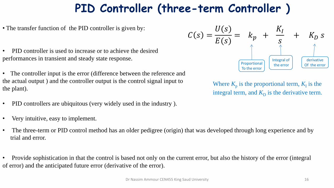
PID Controller (three-term Controller )

• The transfer function of the PID controller is given by:

• PID controller is used to increase or to achieve the desired

performances in transient and steady state response.

• The controller input is the error (difference between the reference and

the actual output ) and the controller output is the control signal input to

the plant).

• PID controllers are ubiquitous (very widely used in the industry ).

• Very intuitive, easy to implement.

• Provide sophistication in that the control is based not only on the current error, but also the history of the error (integral

of error) and the anticipated future error (derivative of the error).

ProportionalTo the error

Integral ofthe error

derivativeOf the error

𝐶 𝑠 =𝑈(𝑠)

𝐸(𝑠)= 𝑘𝑝 +

𝐾𝐼

𝑠+ 𝐾𝐷 𝑠

Where Kp is the proportional term, KI is the

integral term, and KD is the derivative term.

• The three-term or PID control method has an older pedigree (origin) that was developed through long experience and by

trial and error.


PID Controller

• We will examine effect of PID control ( effect of proportional term, derivative term and integral term) on a canonical 2nd order

system to gain insight

• The transfer function of the plant (process) that we wish to control

• The closed-loop transfer function (negative feedback system)


Proportional Control (P)

• The close-loop transfer function

• Control effort is proportional to the amount of error .

the P controller is used in our closed-loop TF. It has a

form similar to a canonical 2nd order system (no zeros,

only two poles).

control signal = constant times the error , so bigger is

the error bigger is the control signal

• Matching with the parameters of a 2nd order canonical system (standard form).

Increasing Kp makes 𝜔𝑛 larger (make the system

stiffer (rigid))

Increasing Kp makes 𝜉 smaller (decreasing the

damping)

• Cannot set 𝜔𝑛 and 𝜉 independently (one d.o.f only one parameter to tune).

• We will see the effect of P control on transient performance


Proportional Control (P) • Effect of P control on steady-state performance

Steady -state value for a unit step reference. We apply the final value theorem to the output Y(s) of our close-loop system

• The poles are all in the left side of the s-plane because all the coefficients of the characteristic equation have the same sign

Transfer function

Unit step input

• The final value of the system does not go to one (with P control we will have

Some amount of error for unit step reference).

• In order to reduce the steady-state error we must increase Kp.

• if we increase Kp to reduce the steady-state error we introduce other adverse

effects such as increasing the overshoot with the oscillation in the performance of

he system. Dr Nassim Ammour CEN455 King Saud University 19

Example

𝐾𝑃 1 10

𝑠2 + 0.05 𝑠

T𝜃𝑑 𝜃+-

The plant is a rotating mass with inertia J=10, the viscous friction b=0.5. To command the position 𝜃 the torque T is used, Find 𝐾𝑃

for a proportional control to have 𝜉 = 0.7.

𝐶𝐿𝑇𝐹 =

𝐾𝑃10

𝑠2 + 0.05 𝑠

1 + 𝐾𝑃10

𝑠2 + 0.05 𝑠

= 𝐾𝑃10

𝑠2 + 0.05 𝑠 + 𝐾𝑃10

𝐶𝐿𝐶𝐸 = 𝑠2 + 0.05 𝑠 + 𝐾𝑃10

𝐶𝐿𝐶𝐸 𝑑𝑒𝑠𝑖𝑟𝑒𝑑 = 𝑠2 + 2𝜉𝜔𝑛𝑠 + 𝜔𝑛2

Matching

For 𝜉 = 0.7

0.05 = 2𝜉𝜔𝑛 = 2 0.7 𝜔𝑛

𝐾𝑃10 = 𝜔𝑛

2

𝜔𝑛 =0.05

2(0.7)= 0.0357

𝐾𝑃 = 10 (0.0357)2= 0.0127

We have the close-loop transfer function:

For proportional control we have: 𝑇 = 𝐾𝑃 (𝜃𝑑 − 𝜃)


Proportional-Derivative Controller (PD)• We will see the effect of adding a derivative action to our P controller


• With derivative control, do not have to wait for error to get large before control action becomes large, control anticipates the

error (by using the slope of the variation of the error and even error is relatively small the control signal increase before the error

gets large, so large control signal, and then improve damping).

• Never use D control by itself, amplifies noise (for D control we use PD or PID).

• The PD controller has a constant proportional to the error plus the proportional (constant KD) to

the differentiation of the error (the term s).

• Substituting in the close-loop controller

• Not canonical form (because of the zero in the numerator), but

trends are meaningful (we can use this transfer function to build

some insight and see the effect of the controlling gains). KD affects sigma term 𝜉with 𝜔𝑛 term

Kp affects 𝜔𝑛

• Can place two poles anywhere (by tuning two parameters Kp and KD gaind, 2 d.o.f)

• If we apply the final value theorem to see the effect on the steady-state error we obtain the same affect as the proportional

control by itself, so the addition of the derivative action didn’t improve the steady-state error.

• Often, Kp is used first to increase the speed of the system and reduce the steady-state error through its effect on 𝜔𝑛, and then

KD is used to bring down the overshoot through its effect on 𝜉. Dr Nassim Ammour CEN455 King Saud University 21

ExampleThe plant G(s) is given in figure, use a PD controller to have the desired system

response 𝜔𝑛 = 4𝑟𝑎𝑑

𝑠𝑎𝑛𝑑 𝜉 = 0.2

𝐺 𝑠 =1

𝑠2 + 𝑠

• The open-loop system poles are 0 and -1, it did not meet the desired specifications, we need to add a controller to have a new system.

For 𝜔𝑛 = 4

𝜉 = 0.2Poles at −8 ± 3.9 𝑖 (using 𝑠2 + 2𝜉 𝜔𝑛 s + 𝜔𝑛

2 = 0)

-1

𝐷𝑒𝑠𝑖𝑟𝑒𝑑 𝑝𝑜𝑙𝑒𝑠

𝑝𝑙𝑎𝑛𝑡 𝑝𝑜𝑙𝑒𝑠

−0.8

3.9

1

𝑠2 + 𝑠𝐾𝑃 + 𝑠𝐾𝐷

𝑋𝑑 𝑋+

−

PD controller Plant

𝐶𝐿𝑇𝐹 =𝐾𝑃 + 𝑠𝐾𝐷 (

1𝑠2 + 𝑠

)

1 + 𝐾𝑃 + 𝑠𝐾𝐷 (1

𝑠2 + 𝑠)=

𝐾𝑃 + 𝑠𝐾𝐷

𝑠2 + 𝑠 + 𝐾𝑃 + 𝑠𝐾𝐷𝐶𝐿𝐶𝐸 = 𝑠2 + 𝑠 + 𝐾𝑃 + 𝑠𝐾𝐷 = 0

𝑠 + 0.8 + 3.9𝑖 𝑠 + 0.8 − 3.9𝑖 = 0


Example

𝐶𝐿𝐶𝐸 = 𝑠2 + (1 + 𝐾𝐷)𝑠 + 𝐾𝑃 = 0

𝐷𝑒𝑠𝑖𝑟𝑒𝑑 𝐶𝐿𝐶𝐸 = 𝑠2 + 1.6s + 16 = 0

Matchingcoefficients

1.6 = 1 + 𝐾𝐷

16 = 𝐾𝑃

𝐾𝐷 = 0.6

𝐾𝑃 = 16

𝑠2 + 2𝜉 𝜔𝑛 s + 𝜔𝑛2 = 0

𝑠2 + 2(0.2) 4 s + 42 = 0desired 𝑠2 + 1.6s + 16 = 0

• For the design we need to find the values of 𝐾𝑃 and 𝐾𝐷 such that the new system satisfies the design criteria. For second order system we have the characteristic equation (not canonical because of the zero in the numerator but a good start)


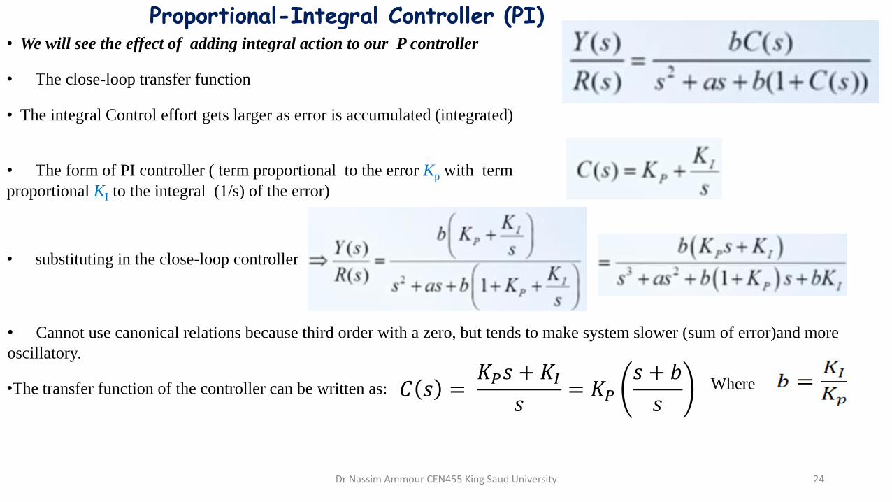
Proportional-Integral Controller (PI)• We will see the effect of adding integral action to our P controller


• The integral Control effort gets larger as error is accumulated (integrated)

• The form of PI controller ( term proportional to the error Kp with term

proportional KI to the integral (1/s) of the error)

• substituting in the close-loop controller

• Cannot use canonical relations because third order with a zero, but tends to make system slower (sum of error)and more

oscillatory.

•The transfer function of the controller can be written as: Where𝐶 𝑠 =𝐾𝑃𝑠 + 𝐾𝐼

𝑠= 𝐾𝑃

𝑠 + 𝑏

𝑠


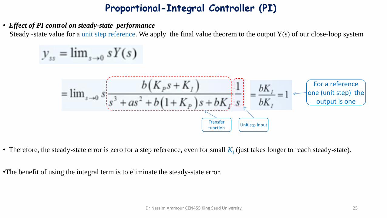
Proportional-Integral Controller (PI)

• Effect of PI control on steady-state performance

Steady -state value for a unit step reference. We apply the final value theorem to the output Y(s) of our close-loop system

• Therefore, the steady-state error is zero for a step reference, even for small KI (just takes longer to reach steady-state).

Transfer function

Unit stp input

For a reference one (unit step) the

output is one

•The benefit of using the integral term is to eliminate the steady-state error.


ExampleThe plant G(s) is given, use a PI controller to have the desired system response:

𝜉 = 0.7, 𝑇𝑠 < 1𝑠, 𝑒𝑠𝑠 = 0 𝑓𝑜𝑟 𝑠𝑡𝑒𝑝 𝑟𝑒𝑠𝑝𝑜𝑛𝑠𝑒

𝐺 𝑠 =10

𝑠 + 3

𝑅𝑒𝑞𝑢𝑖𝑟𝑒𝑑 𝑎𝑟𝑒𝑎 𝑓𝑜𝑟𝑡ℎ𝑒 𝐷𝑒𝑠𝑖𝑟𝑒𝑑 𝑝𝑜𝑙𝑒𝑠

𝑝𝑙𝑎𝑛𝑡 𝑝𝑜𝑙𝑒

−4

• The desired system poles:

• The plant poles: -3

𝑇𝑠 =4

𝜎< 1 → 𝜎 > 4

𝑅𝑒

𝐼𝑚

−3

• The open-loop system did not meet the desired specifications, we need to add a controller to have a new system.

10

𝑠 + 3𝐾𝑃 +𝐾𝐼

𝑠

𝑋𝑑 𝑋+

−

PI controller Plant

𝐶𝐿𝑇𝐹 =𝐾𝑃 +

𝐾𝐼𝑠 (

10𝑠 + 3)

1 + 𝐾𝑃 +𝐾𝐼𝑠 (

10𝑠 + 3)

=10 𝐾𝑃𝑠 + 𝐾𝐼

𝑠2 + 3𝑠 + 10 𝐾𝑃𝑠 + 𝐾𝐼𝐶𝐿𝐶𝐸 = 𝑠2 + (10𝐾𝑃 + 3)𝑠 + 10𝐾𝐼 = 0


• using Matlab we can find the values of 𝐾𝑃 and 𝐾𝐼 to put the poles in the desired area to meet the design specifications.

Matchingcoefficients

2𝜉 𝜔𝑛 = 10𝐾𝑃 + 3

𝜔𝑛2 = 10 𝐾𝐼𝐶𝐿𝐶𝐸 = 𝑠2 + (10𝐾𝑃 + 3)𝑠 + 10𝐾𝐼 = 0

𝑠2 + 2𝜉 𝜔𝑛 s + 𝜔𝑛2 = 0

𝑇𝑠 =4

𝜉 𝜔𝑛< 1 𝜔𝑛 >

4

0.7= 5.71

𝐾𝐼=𝜔𝑛

2

10> 3.27

We have 𝜉 = 0.7

𝐾𝑃 >2𝜉 𝜔𝑛 − 3

10≈ 0.5

𝐾𝐼 = 4

𝐾𝑃 = 0.6For


PID Control

• Increasing Kp : Same amount of error generates a proportionally larger amount of control, makes system faster, but overshoot more (less stable).

•Increasing KD : Allows controller to anticipate an increase in error, adds damping to the system (reduce overshoot), can amplify noise.

• Increasing KI : Control effort builds as error is integrated over time, helps reduce steady-state error, but can be slow to respond.

3. Following table is helpful, though not always true

2. For systems that are not canonical first or second order, need to use trial and error. Can look for reduced-order approximation ( try to identify if there are any poles that dominate the response, try to identify if there are any of zeros cancel with any of the poles, and if we can take a higher order system and approximates it as first or second order system.

1. Some intuition about the effect of the PID terms.


controller design by pole placement - fac.ksu.edu.sa · the calculated gains will be a good...

Documents