Convenient Estimators for the Panel Probit Model: Further Results

William Greenea*

aDepartment of Economics, Stern School of Business, New York University, 44 West 4th St., New York, NY, 10012, USA.

Revised, October, 2002

________________________________________________________________________ Abstract Bertschek and Lechner (1998) propose several variants of a GMM estimator based on the period specific regression functions for the panel probit model. The analysis is motivated by the complexity of maximum likelihood estimation and the possibly excessive amount of time involved in maximum simulated likelihood estimation. But, for applications of the size considered in their study, full likelihood estimation is actually straightforward, and resort to GMM estimation for convenience is unnecessary. In this note, we reconsider maximum likelihood based estimation of their panel probit model then examine some extensions which can exploit the heterogeneity contained in their panel data set. Empirical results are obtained using the data set employed in the earlier study. JEL classification: C14; C23; C25 Keywords: Panel probit model; Multivariate probit; GMM; Simulated likelihood; Latent class; Marginal effects ________________________________________________________________________

* E-mail: wgreene@stern.nyu.edu. Helpful comments and suggestions by Irene Bertschek and Michael Lechner are gratefully acknowledged. Any remaining errors are the responsibility of the author.

1

1. Introduction Bertschek and Lechner (1998) (henceforth BL) propose a set of “convenient”

GMM estimators for the binomial probit model based on panel data. Their GMM

approach is motivated by the difficulty of computation of the log likelihood function for a

fully unrestricted model with freely correlated disturbances when there are T > 2 time

periods. Because of the need to use a simulation based estimator, the primary obstacle is

the actual amount of computation. They also argue that estimation of the disturbance

covariance matrix, which involves T(T-1)/2 free parameters, is unattractive because of the

large size of the estimation problem. This note will compare the full likelihood based

estimator to their GMM estimator. Speeds of computation have improved to the point

that for a problem of the size of their application, the issue of computation time that was a

focus of the earlier article is a minor consideration. More importantly, estimation of the

full covariance matrix is revealing about the structure of the model in a way that would

not be evident from their GMM approach. We will also examine two extensions of the

panel probit model that were not considered by BL. The panel data set provides

information about individual heterogeneity that is not exploited by the GMM estimator.

We will reexamine their data set in the context of a random parameters model and a latent

class model, both of which provide a means of examining the individual heterogeneity.

The random parameters model has been widely used in the discrete choice (multinomial

logit) framework, but has seen very limited application in the probit model, and none in

the form considered here. The latent class model h as been used almost exclusively to

study count data. It appears not to have been employed previously in the analysis of

binary choice data.

Section 2 of this paper describes the maximum likelihood and GMM panel data

parameter estimators. Section 3 discusses the common effects models and two

extensions of the probit model, random parameters and latent classes. The application is

described in Section 4.1 Some conclusions are drawn in Section 5. The random

parameters model is estimated using a quasi Monte Carlo simulation method that has not

1 The authors of the earlier study have generously allowed us to reuse their data for this analysis. Their assistance is gratefully acknowledged.

2

yet seen wide use in econometrics. Some notes on this technique are provided in the

appendix.

2. Estimation of the Panel Probit Model The panel probit model is

(1) 0 , 1,..., , 1,..., ,

( 0).it it it

it it

y t T i

y y

∗

∗

′= + ε = =

= >

x1

β N

T

The data consist of N observations on Zi = (yi,Xi) where yi = (yi1, yi2, …., yiT)′ and the T

rows of the T×K matrix Xi are The disturbances T-variate normally

distributed with T×T positive definite covariance matrix Σ. The typical element of Σ is

denoted σ

, 1,..., .it t′ =x

ts. The standard deviations, ttσ are denoted σt. The data on xit are assumed

throughout to be strictly exogenous, which implies that Cov[xit,εjs] = 0 across all

individuals i and j and all periods t and s. This rules out state persistence, or the presence

of lagged dependent variables in (1).2

2.1. Specification, Identification and Restrictions

The model in (1) is a special case of the M equation multivariate probit model

(2) 0 , 1,..., , 1,..., ,

( 0)im im m im

im im

y m M i

y y

∗

∗

′= + ε = =

= >

x1

β N

in which the parameter vectors are identical across equations.3 The observed data contain

no information on the scaling of y*, so the diagonal elements of Σ, σtt, are usually

normalized to one. In the model in (1), however, normalization of all the diagonal

elements is unnecessary because the slope vector is time invariant; T-1 ratios, σ1/σt are

identified. As noted by BL, then, only one main diagonal element of Σ, σ11, is

normalized to one for identification purposes - β0 is identified only “up to scale.” Since

the scaling may be different across periods, an equivalent formulation of (1) which

2 See Heckman (1981) and Wooldridge (1995) for discussion. 3 This is an M-variate extension of the bivariate probit model used, e.g., in Rubinfeld (1983), Boyes, Hoffman and Low (1989), Greene (1992), Burnett (1997) or Greene (1998).]

3

embodies the convenient normalization σtt = 1 while not restricting the variance

parameters is obtained by scaling the coefficient vectors, instead;

(3)

0 0 , 1,..., , 1,..., ,

( 0).it it t it

it it

y t T i

y y

∗

∗

′= θ + ε = =

= >

x1

β N

where = σ0tθ 1/σt. The normalization imposed by BL, σ11 = σtt = σTT - see their footnote

2 on page 332 - is therefore restrictive.4 It is equivalent to an assumption that = 1, t =

2,…,T, or that the disturbances are homoscedastic through time. While the assumption is

substantive, for the data in their application, it does appear to be reasonable. The scale

parameters are identified (estimable), so in principle, the restriction could be tested in

a given application.

0tθ

0tθ

5 Since the null hypothesis in this case is simply = 1 for t > 1, the

test can easily be carried out in either the GMM or ML framework by fitting the model

without the restriction of equal parameter vectors. Hansen’s (1982) J test or the

likelihood ratio test can be used. An application appears below in Section 4.

0tθ

2.2. Pooled and Random Effects Estimation The most restrictive estimation approach assumes away all the cross period

correlation and treats the panel essentially as a cross section. This produces the “pooled”

estimator which is the standard, single equation probit model found in any econometrics

text. The “random effects” model analyzed by Butler and Moffitt (1982) maintains the

homoscedasticity (unit variances) assumption but extends the pooled model by allowing

cross period correlation, in their case, equal for all period pairs. Under the general

(unrestricted multivariate normality) specification in (3) with θ = 1, both these

estimators are consistent but inefficient. (Both are special cases of the GMM estimator

proposed by BL.) However, the conventionally estimated standard errors that accompany

0t

4 BL do consider an equivalent but less convenient normalization in their footnote 2 (p. 332). We will retain this normalization in what follows. 5 This will require a full information maximum likelihood estimator, such as the one suggested here. BL’s development was focused primarily on GMM estimators which obviate the calculation of Σ.

4

each are inappropriate as they ignore the unrestricted cross period correlation.6

Butler and Moffitt’s random effects probit model specifies εit = uit + vi where uit is

normally distributed with mean zero and is independent across all periods and individuals

and assumes that the individual specific term, vi is uncorrelated with the included

variables xit in all periods, is independent across individuals, and is time invariant. This

produces the modified covariance matrix σts = σv2/(σu

2+σv2) = ρ for t ≠ s and σtt = σv

2 +

σu2 = 1 on the main diagonal of Σ. In this case, the model contains only β plus one

additional correlation parameter, ρ. The log likelihood may be maximized by Hermite

quadrature or by simulation methods.7 (Some details are given by BL.)

2.3. Maximum Likelihood Estimation

Full maximum likelihood estimates of the parameters in (3) with the

homoscedasticity assumption are obtained by maximizing the log likelihood function,

( )

1 21

log log ( , ,..., | *)N

Ti i iT

iL a a a

=

= Φ∑ Σ (4)

with respect to the unknown elements in β and Σ where, σtt = 1, ait = (2yit – 1)xit′β, σts*

= (2yit – 1)(2yis – 1)σts, t ≠ s, and Φ(T) denotes the CDF of the T-variate normal

distribution. (The restriction, θ =1 has already been imposed.) When T exceeds two,

computation of this function requires a multidimensional integration which can only be

approximated. This can be done by simulation methods. The GHK simulator was used

here.

0t

8 BL note three obstacles to estimation of this model: first, the amount of

computation seems to be excessive (“prohibitively high”), which for their application is

6 The moment equations for both estimators are based on the correct marginal conditional mean assumption, which induces the consistency. But, in each case, the asymptotic covariance matrix estimated from the assumed Hessian is not based on the actual joint density of the observations. White’s (1982) results would apply here, so a ‘sandwich’ estimator based on both the (assumed) Hessian and the BHHH estimator would give appropriate standard errors. 7 The fixed effects (dummy variables) model is an alternative approach that might be considered if vi were assumed to be correlated with xit. However, this estimator for the probit model is known to be inconsistent in a panel as short as ours (T = 5) due to the incidental parameters problem. Moreover, it precludes time invariant regressors, and the model considered here has two. See Greene (2002) for analysis of the fixed effects model. 8 See Hajivassiliou and Ruud (1994), Hajivassiliou et al., (1996), Geweke et al. (1994, 1997) and Geweke (1997).

5

actually not the case - see the application below; second, global concavity may be a

problem; and third, there are a large number of nuisance parameters in the model. BL’s

analysis produced several strategies for estimation designed to circumvent estimation of

the off diagonal elements of Σ. But, in the application below, the estimated elements of Σ

are actually revealing in terms of suggesting a useful simplification of the model.

243. GMM Estimation

BL suggest a set of GMM estimators based on the orthogonality conditions

implied by the single equation conditional mean functions;

(5) [ ( )] | 0it it iE y ′− Φ =x Xβ where Φ denotes the CDF of the univariate normal distribution. The orthogonality

conditions are

(6)

1 1

2 2

[ ( )][ ( )]

( )

[ ( )]

i i

i ii

iT iT

yy

E

y

′ − Φ ′− Φ = ′− Φ

xx

A X 0

x

ββ

β

.

Using only the raw data as A(Xi), where A(Xi) is a P×T matrix of instrumental variables

constructed from the exogenous data for individual i, strong exogeneity of the regressors

in every period [see Wooldridge (1995)] would provide TK moment equations of the

form E[xit(yis-Φ(xis′β))] = 0 for each pair of periods, or a total of T2K moment equations

altogether for estimation of K parameters in β. The full set of such orthogonality

conditions would be E[(IT ⊗ xi)ui] = 0 where xi = [ ,..., ]′, u1i′x iT′x i = (ui1,…,uiT)′ and uit =

yit - Φ(xit′β). For BL’s application, (6) produces 200 orthogonality conditions for the

estimation of the 8 parameters.9 The empirical counterpart to the left hand side of (6) is

9 See Ahn and Schmidt (1995) and Arellano and Bover (1995) for discussion. BL constructed a different set of instruments, but did not use the strong exogeneity assumption. Their set of instruments used the current period orthogonality conditions in (7), so the total number of restrictions employed was TK. An expanded set of instruments based on the weak exogeneity assumption was examined in Breitung and Lechner (1997). Such vastly overidentified GMM estimation problems bring new (bias) problems of their own – see Ahn and Schmidt (1995) for discussion.

6

( )

1 1

2 2

1

[ ( )][ ( )]1 ( )

[ ( )]

i i

Ni i

N ii

iT iT

yy

Ny

=

′ − Φ ′− Φ = ′− Φ

∑

xx

g A X

x

ββ

β

β

.

β

(7)

The various GMM estimators are the solutions to

. ( ) ( ), , arg minGMM N N′ A W g W g

ββ = β

The specific estimator is defined by the choice of instrument matrix A(Xi) and weighting

matrix, W; the authors suggest several. BL assumed strong exogeneity of the regressors

in their application (see p. 337), so that in the construction of (6), only data from period t

are used in the tth moment condition. This reduces the number of moment conditions

from 200 to 40, which is the same number used by the MLE. Further details on

computations appear in their paper and in the application below.

All of the preceding is done without (i.e., so as to avoid) direct full estimation of

the matrix Σ.10 Thus, the various estimators suggested attain their relative efficiencies

within the class of GMM estimators, but all are inefficient relative to the full MLE

implied by (4)11. We do note that the GMM estimator in this application is somewhat

unlike many other treatments in that by comparison to the MLE, because of the strong

exogeneity assumption, it does not involve additional moment equations. The moment

equations are based on the marginal conditional means in (3) whereas the MLE is based

on the joint density in (4). Robustness of the GMM estimator in this setting would come

about through its possibly less restrictive distributional. The full MLE assumes T-variate

normality for the disturbances in (2). The various GMM estimators suggested by BL

10 A considerable amount of the derivation in the paper concerns approximations to Var[ NN g ]. One additional simple estimator which was not examined would be the sample second moment matrix of the terms in gN based on any consistent first round estimator of β, of which several were suggested. This estimator was considered in Breitung and Lechner (1997) and found to be inferior to the analytic estimator because of the very large number of overidentifying restrictions. 11 One could argue that (7) is based only on the specified conditional mean functions and not on normality at all. However, this would necessitate contriving some other motivation for this particular conditional mean function and, in addition, would greatly complicate the formulation of a weighting matrix based on the covariances of the orthogonality conditions.

7

assume marginal normality for each disturbance in (2) and correlation across equations.

Whether the various suggested structures are substantially less restrictive is unclear. For

example, assuming that each pair of disturbances has a bivariate normal density, as BL do

in their (15) does not imply joint normality for the set, but in practical terms, it seems

unlikely that the assumption would leave much room for variation from the stronger

assumption.12 Thus, the difference in the two approaches turns on marginal vs. joint

normality, since both allow free correlation of the disturbances while assuming

homoscedasticity.

2.5. Computation

The authors suggest that the computation time needed to fit this model by full

maximum likelihood is “prohibitively high for T > 4 or 5…” For present purposes, a

simple benchmark is useful. As of their writing, the mid-1990s, their computation of the

“pooled” probit model using their fairly large sample of 1,270×5 observations and eight

regressors took 30 seconds. (See their page 363.) The same computation using the same

data on a less than leading edge personal computer in 2002 took less than 0.3 seconds, a

more than 100 fold improvement.13 A similar comparison relates to a first step

estimation of the elements of Σ, which can be done in principle by fitting a set of

bivariate probit models. The authors deem this calculation “cumbersome for large T,”

but, for their sample of N = 1,270 observations, computation of each bivariate probit

model takes less than six seconds. The upshot is that computation time and “burden” for

maximum likelihood and the simulation estimators, which is a recurrent theme in the BL

study and one of the primary motivations for the “convenient estimators” should now be

well within the acceptable range for many problems. We have fit the multivariate probit

model in (3) using the full information maximum simulated likelihood estimator. The

amount of computation is large, but not excessive. Estimation was fairly routine, and

12 Joint normality would require that every linear combination of the εs be normally distributed. See Greene (2003, Theorem D18A, p. 912). 13 The authors used Gauss© for their computations. Results in this paper were obtained with Version 8.0 of LIMDEP©.

8

took altogether under an hour on a 1.66 Ghz personal computer.14 Full estimation results

and details are given below.

3. Alternative Forms and Estimators for the Panel Probit Model The panel data set used by BL contains a considerable amount of between group

variation. For example, based on a simple analysis of variance, 97.6% of the variation in

the FDI variable and 92.9% of that of the imports share variable are accounted for by

differences in the group means. With the exception of the Butler and Moffitt random

effects formulation, the approaches suggested do not model the heterogeneity that is

likely to be present in a data set of this sort. Several approaches might be considered.

Butler and Moffitt’s random effects probit model was proposed to allow persistent

unobserved individual heterogeneity to enter the model. The equicorrelation structure

that results is a consequence of the assumptions about the heterogeneity term, vi – time

invariant and strongly exogenous – not a deliberate feature of the multivariate probit

model.. We have merely adapted it as such in the preceding derivations as a convenient

device to restrict the more general model. However, panel data such as these do provide

a platform on which to analyze individual heterogeneity. Viewed from this perspective –

that is cross unit heterogeneity rather than simple cross period correlation, the model in

(3) turns out, itself, to be restrictive. In this context, the cross period correlation could be

viewed as induced by latent, persistent individual heterogeneity, which would precisely

reproduce the Butler and Moffitt model. We now consider some alternative

specifications. Two alternative formulations that have been widely used to analyze panel

data in other contexts, but not in the probit model, are the random parameters model and

14 Computation times are difficult to compare in the current changing computing environment. For the multivariate model discussed below, as noted in the text, the full MLE does require much more computation than the GMM estimator. The amount of computation is roughly quadratic in T and linear in N, the number of observations and R, the number of replications for the simulations. The model size, K, is a minor contributor to the total because by far the majority of the computation effort involves simulating the T-variate probabilities. The practical limit of the GHK simulator suggested by received applications appears to be about 10 periods. A model this large (T = 10), with a reasonable number of replications (say R = 100) could likely take many hours to estimate with current (2002) technology, and accuracy of the integration would be suspect in any event. But, for problems of the scale considered here, especially with the most up to date computers, computation of the multivariate probit model is not likely to be prohibitive.

9

the latent class model.15

An alternative formulation of (1) is

(8) 0 ( ) , 1,..., , 1,..., ,

( 0).it it it it

it it

y v t T i

y y

α∗

∗

′= + + ε = =

= >

+ x1

β N

)

i

where εit is normally distributed with zero mean and is uncorrelated across time and

individuals and vit has zero mean and is freely correlated and heteroscedastic across time

but independent across individuals. The homoscedasticity restriction would be imposed

as before by σvt2 = σv

2. This reproduces the original model, but from a different

perspective, that of latent heterogeneity, embodied in a random constant term. (The

underlying specification issue to be resolved is what process induces the correlation

across time.) Butler and Moffitt’s model results if vit is time invariant, as vi. Allowing the

other parameters in the model to be random as well produces the next two models

considered.

3.1. A Random Parameters Model

The random parameters (or ‘hierarchical’ or ‘multilevel’) model is an extension of

(8),

, 1,..., , 1,..., ,it it i ity t T i∗ ′= + ε = =x β N ~ [0,1]it NIDε

(9) ( 0it ity y∗= >1

where i i= + +z wβ µ ∆ Γ

µ = K×1 vector of unconditional means ∆ = K×L matrix unknown location parameters, Γ = K×K lower triangular matrix of unknown variance parameters,

15 A restricted form of the random parameters probit model analyzed here was examined by Akin, Guilkey and Sickles (1979), Guilkey and Murphy (1993) and Sepanski (2000). The random effects model is also a special case which has been applied in a number of applications. An extensive analysis of the random parameters logit model is Train (2002). Comments also appear in McFadden and Train (2000).

10

zi = L×1 vector of individual characteristics wi = K×1 vector of random latent individual effects with E[wi|Xi,zi] = 0 Var[wi|Xi,zi] = V = K×K diagonal matrix of known constants. It follows that E[βi|Xi,zi] = µ + ∆zi and (10) Var[βi|Xi,zi] = ΓVΓ′ = Ω. The distribution of βi is induced by that of wi and remains to be specified. Since Γ need

not be diagonal, in principle, the distribution could be a complicated mixture of diverse

components. If wi is assumed to have a standard, spherical normal distribution, then βi

will be normally distributed with the moments given above. We use the Cholesky

factorization to form the covariance matrix of the random parameters. The covariance

matrix of wi is assumed known and diagonal, since any unknown parameters will be

absorbed in Γ. In most cases, when it is assumed that the random parameters are

normally distributed across individuals, V will be an identity matrix. It is not necessary

to assume normality – infinite range of variation may be implausible for certain

parameters. As such, the diagonals of V might take other values. For example, if the

variation of a parameter is assumed to follow a uniform distribution, then the

corresponding value of V would equal 1/12 and the unknown scaling would be accounted

for by the corresponding elements in Γ.

The mean vector in the random parameters model is formulated with a vector of

time invariant, individual specific variables zi. When present, the unknown coefficients

are contained in the corresponding row of ∆. Nonrandom parameters in a model are

specified by imposing the constraint that the corresponding rows of Γ contain zeros.

Allowing nonzero rows in ∆ while constraining the corresponding row in Γ to be zero

provides a convenient means of formulating a ‘hierarchical’ model. The original random

effects panel data model examined in the preceding section is produced by including in

the model a simple random constant term. (The firm specific mean terms, ∆zi will not be

11

present.) The dynamic effects are more difficult to accommodate. One possibility is to

generate wit by a stochastic process, such as an AR(1). Thus, as opposed to the time

invariant effects model, the preceding can be made dynamic by allowing wit to equal

Rwi,t-1 + hit where R is a diagonal matrix of autocorrelation coefficients to be estimated

with the other model parameters and hit is the white noise process. [See Greene (2002).]

Other stochastic processes could be accommodated as well.

The random parameters model may be estimated by maximum simulated

likelihood or by Markov Chain Monte Carlo (MCMC) methods.16 Conditioned on wi,

observations on yit are independent across time – timewise correlation per the focus of

this paper would arise through correlation of elements of βi. The joint conditional density

of the T observations on yit is

(11) ( ) [1

| , (2 1)T

i i i it it it

f y=

′= Φ −∏y X xβ ].β

i idz

The contribution of this observation to the log likelihood function for the observed data is

obtained by integrating the latent heterogeneity out of the distribution. Thus,

(12) [ ]

1 1 1

log log log (2 1) ( | , , , )i

TN N

i it it i ii i t

L L y g= = =

′= = Φ −∑ ∑ ∏∫ xβ

β β µ ∆ Γ β

Full information maximum likelihood estimates of the parameters µ, ∆, Γ are obtained by

maximizing this function. Since the function involves multidimensional integration,

direct optimization is generally not feasible. Maximum simulated likelihood is used

instead. The simulated log likelihood is

[1 1 1 1

1log log log (2 1)TN N R

s is iti i r t

L L yR= = = =

′= = Φ −∑ ∑ ∑∏ x β ]it ir

iw

(13)

where βir is the rth of R simulated draws on from the underlying

distribution of w

i i= + +zβ µ ∆ Γ

i. Estimates of µ, ∆, and Γ are obtained by maximizing the simulated log

likelihood function.17 Observations on βir are constructed from primitive draws on wi.

16 See, Train (2002), Greene (2003, Chapter 16), or Albert and Chib (1993). 17 See Gourieroux and Monfort (1996) and Train (2002) for discussion.

12

Note that it is not necessary to assume normally distributed parameters. The integration

by simulation simplifies the computations in such a way that other distributions are easily

accommodated. For example, the range of variation can be restricted by using a “tent” or

uniform distribution, either of which is easily simulated. The estimated elements of Γ will

carry the sample information on the range of variation. A more complete exposition in

the context of logit models for discrete choice appears in Train (2002) and in general

terms in Greene (2001). Maximum simulated likelihood estimation is extremely

computation intensive. The process is speeded up by using a quasi-Monte Carlo method

based on Halton sequences of draws instead of random draws using a random number

generator. The method is described in the appendix.

With estimates of the structural parameters (µ, ∆,Γ) in hand, estimates of the

individual specific parameter vectors may be obtained by the posterior mean

[ ][ ]

[ ]

1

1

(2 1) ( | , , , )ˆ | , , , , ,

(2 1) ( | , , , )

i

i

T

i it it i i it

i i i i i T

it it i i i it

y gE

y g

=

=

′Φ − = = ′Φ −

∏∫

∏∫

x zy X z

x z

β

β

β β β µ ∆ Γµ ∆ Γ

β β µ ∆ Γ β

id

d

ββ β (14)

[See Train (2002), Chapter 11.] The parts can be estimated by simulation. The

application below demonstrates.

3.2. A latent Class, Finite Mixture Model The latent class model can be motivated from several perspectives. One can view

the formulation as an alternative specification of the random parameters model. The

model in Section 3.1 assumes that βi is continuously distributed across firms in the

population. We might assume a discrete distribution instead. The discrete distribution

can be viewed as the model in its own right, or as a semiparametric approximation to an

underlying, continuous distribution. Alternatively, the latent class model can be viewed

as arising from a discrete, unobserved sorting of individuals (firms) into groups, each of

which has its own set of characteristics. This implies that the observed sample is

comprised of a discrete mixture of individuals of different types. Finally, we may view

the discrete mixture, itself, as a flexible structural model which is much less restrictive

13

than the singly parameterized probit equation. Finite mixtures as an approach to flexible

modeling of random variables has a long history in many fields. [See, e.g., McLachlan

and Peel (2000) for an exhaustive survey.] All these interpretations produce the same

structure.

Assuming independence across time, the conditional density for the observed data for individual i is

( ) [ ]1

| , (2 1)T

i i i it it it

f y=

′= Φ −∏y X xβ β .

d

)

In the continuous case examined earlier, the conditional density of the random

parameters, induced by the random vector wi, is g(βi| µ, ∆, Γ, zi). The unconditional

density is the contribution to the likelihood given earlier,

f(yi|Xi, zi, µ,∆,Γ) = = .( )| ,i i i iE f y Xβ β [ ]

1

(2 1) ( | , , , )i

T

it it i i i it

y g=

′Φ −∏∫ x zβ

β β µ ∆ Γ β

The density of βi is the weighting (mixing) distribution in this average. If the distribution

of βi has finite, discrete support over J points (classes) with probabilities p(βj|µ, ∆,Γ,zi), j

= 1,...,J, then the resulting formulation is,

f(yi|Xi, zi, µ, ∆, Γ) = (15)

1( | , ,M

j ijp

=∑ zβ µ, ∆ Γ ) ( | ,i i jf y X β

where it remains to parameterize the regime probabilities, pij.18 (We will arrive at a

discrete distribution that is parameterized in terms of only the matrix ∆, so µ and Γ will

be unnecessary.) Estimation is over the J regime probabilities and the regime level

parameters βj. The class probabilities must be constrained to sum to 1. A simple

approach is to reparameterize them as a set of logit probabilities,

pij = 1

, 1,..., , 0ij

ijiJJ

j

e j Je

θ

θ

=

= θ∑

=

, θij = δj′zi.19 (16)

18 Applications to models for count data may be found in Nagin and Land (1993), Wang Cockburn and Puterman (1998) and Wedel, DeSarbo, Bult, and Ramaswamy. (1993). 19 As noted, this model has appeared in a number of applications to count data. Wedel et al. imposed the adding up constraint on the prior probabilities by a Lagrangean approach. As can be seen above, a simple reparameterization of the probabilities achieves the same end with much less effort. Nagin and Land (1993) and Wang et al. (1998) used the logit parameterization. Brannas and Rosenqvist (1994) forced the probabilities in their model to lie in the unit interval by using the parameterization pj = 1/[1+exp(-θj)] with

14

(Thus, δj′ is the jth row of ∆.) The resulting log likelihood is a continuous function of the

parameters, and maximization is straightforward.

Estimation produces values for the structural parameters, βj, and the parameters of

the prior class probabilities, δj. One might also be interested in the posterior class

probabilities,

Prob(class j | observation i) = 1

(observation | class ) Pr ob(class )(observation | class ) Pr ob(class )J

j

f i jf i j

=∑j

j

= ( )

( )1

| , ( , )

| , ( , )i i j ij i

Mi i j ij ij

f p

f p=∑

y X z

y X z

β ∆

β ∆ (17)

= wij. This set of probabilities, wi = (wi1,wi2,...,wiJ) gives the posterior density over the

distribution of values of β, that is, [β1, β2, ..., βJ]. An estimator of the individual specific

parameter vector would then be the posterior mean

1

ˆ ˆ [ | observation ]J

pi j j ij

jE i

=

= ∑β β ˆjw= β

ˆj jβ

. (18)

As before, the posterior mean , rather than the prior mean , would be used to

make efficient use of al the information in the sample.

0

1

ˆJ

i ij

p=

= ∑β

The EM algorithm is a convenient approach for estimation of this model.20 Let dij

= 1 if individual i is a member of class j and zero otherwise. We treat dij as missing data

to be estimated. The joint density of J dijs is multinomial with probabilities pij;

. (19) 1 2 1( , ,..., | , ) ( | , ) ijJ d

i i iJ i i i ijjf d d d f p

== = ∏z d z∆ ∆

The complete data log likelihood is built from the joint density,

f(yi,di|Xi,zi, ,∆) = f(yi|di,Xi,) f(di|zi,∆).

θj unrestricted. This does solve the problem, but they did not impose the adding up constraint, Σjpj = 1 in their model; they simply estimated the first θ1,...,θM-1 without restriction and computed pM residually, a procedure that is not guaranteed to succeed. 20 See Dempster, Laird, and Rubin (1977), Wedel et al. (1993) and McLachlan and Peel (2000).

15

Thus, logLc = (20)

1 1log ( | , ) logN J

ij i i j ij iji jd f d p

= = + ∑ ∑ y X β

The expectation (E) step of the process involves obtaining the expectation of this log

likelihood conditioned over the unobserved data. This involves replacing the dijs in log

Lc with the posterior probabilities, wij, derived above (computed at the current estimates

of the other parameters). The maximization (M) step then involves maximizing the

resulting conditional log likelihood with these estimated posterior probabilities treated as

known. Conditioned on the posteriors, E[logLc] factors into two parts that may be

maximized separately. By construction, Σjwij = 1. The first part of the log likelihood

becomes a weighted log likelihood with known weights for which the likelihood

equations are

1

log ( | , ) [log ] N i i jciji

j j

fE L w=

∂∂= =

∂ ∂∑y X

0β

β β.

This involves simply maximizing a weighted, pooled log likelihood for each class

parameter vector where the weights are the firm specific posterior class probabilities for

the particular class.. If there are no individual specific variables in the probabilities, then

the maximum likelihood estimators of the class probabilities are just the sample averages

of the estimated weights;

1ˆN

ijij

wp

N== ∑ .

If the logistic parameterization has been used, then the conditional log likelihood function

at the M step for these parameters is a weighted multinomial logit log likelihood, which

will require an iterative solution. The iterative solution for the structural parameters, δj is

the solutions to the likelihood equations

1

[log ] ˆ( )Ncij ij ii

j

E L w p=

∂= −

∂ ∑ zδ

= 0 .

16

This is the first order conditions for the multinomial logit model with proportion rather

than individual data for the dependent variable (the weights). The EM method thus

amounts to cycling between these two steps - computing the parameters for the class

probabilities via the multinomial logit procedure at the second step above, then

recomputing the class specific weighted probit estimators at the first step by a simple

weighted, pooled maximum likelihood probit estimator.

4. Application Bertschek and Lechner applied the GMM estimator to an analysis of the product

innovation activity of 1,270 German manufacturing firms observed in five years, 1984 -

1988, in response to imports and foreign direct investment. [See Bertschek (1995).] The

basic model to be estimated is a probit model based on the latent regression

, , i = 1,...,1270, t = 1984,...,1988. 8

1 ,2

*it k it k it

ky x

=

= β + β + ε∑ ( * 0it ity y= >1 )where yit = 1 if a product innovation was realized by firm i in year t, 0 otherwise, x2,it = Log of industry sales in DM, x3,it = Import share = ratio of industry imports to (industry sales plus imports), x4,it = Relative firm size = ratio of employment in business unit to employment in the industry (times 30), x5,it = FDI share = Ratio of industry foreign direct investment to (industry sales, plus imports), x6,it = Productivity = Ratio of industry value added to industry employment, x7,it = Raw materials sector = 1 if the firm is in this sector, x8,it = Investment goods sector = 1 if the firm is in this sector, Descriptive statistics and further discussion appear in the earlier papers. Their primary

interest was in the effect of imports and inward foreign direct investment on innovation.

Both are hypothesized to have a positive effect. We have extended the analysis with their

data.

Table 1 presents the base case, “pooled” estimator. This is the simple probit

estimator that treats the entire sample as if it were a large cross section. This estimator is

consistent, but inefficient. Four sets of asymptotic standard errors are presented with the

estimates. The first are BL’s reported standard errors. These are computed using a

robust estimator based on White (1982). [See their pp. 345 and 359.) The second set are

17

the square roots of the diagonals of the negative of the inverse of the Hessian computed at

the maximum likelihood estimates (which we have reproduced). The third set are those

computed by BL based on Avery, Hansen and Hotz’s (1983) GMM estimator. [See BL

(1998, pp. 338-339).] A natural alternative which should be appropriate in this setting is

the so-called “cluster” estimator [see Stata (1998)]:

( ) ( ) ( )1 1

1

1

ˆˆ1

n

i ii

T

i itt

NN

− −

=

=

′= − − −

=

∑

∑

V H g g

g g

β H (21)

The matrix H is the conventional Hessian of the maximized log likelihood and git is the

derivative of the individual term in the pooled log likelihood. As can be seen in Table 1,

the cluster estimator produces essentially the same results as the GMM based estimator.

The last two columns of Table 1 present the estimated partial effects of the variables on

the probability of a realized innovation. Standard errors are based on the cluster

estimator and are computed using the delta method. [See Greene (2003, chapter 19).]

The estimates for the sector dummy variables are computed by evaluating the probability

at the means of the other variables and with the dummy variables equal to one then zero -

the marginal effect in each case is the difference. The results thus far are consistent with

the hypothesis that imports and FDI positively and significantly affect product

innovation.

Table 2 reports the estimates of the random effects (equicorrelated) model. The

random effects model was fit by two methods, first using Butler and Moffitt’s method

with a 32 point Hermite quadrature, then by specifying the random parameters model

with only a random constant term. In terms of the estimates of the parameters, it is clear

that, as expected, the two integration methods produce essentially the same results. The

random parameter estimator produced an estimate of the standard deviation for the

random constant of 1.1707. Based on the normalization σv2 + σu

2 = 1, this produces an

estimator of the correlation coefficient of 1.17072 / (1 + 1.17072) = 0.578, which is

identical to the estimate produced by the quadrature method. The value itself is also

striking, as will be evident in the next set of results for the multivariate probit model.

18

Table 1. Estimated Pooled Probit Model Estimated Standard Errors Marginal Effects Variable Estimatea se(1)b se(2) c se(3)d se(4)e Partialf Std. Err. Constant -1.960** 0.21 0.230 0.377 0.373 log Sales 0.177** 0.025 0.0222 0.0375 0.0358 0.0683 0.0138** Rel Size 1.072** 0.21 0.142 0.306 0.269 0.413 0.103** Imports 1.134** 0.15 0.151 0.246 0.243 0.437 0.0938** FDI 2.853** 0.47 0.402 0.679 0.642 1.099 0.247** Prod. -2.341** 1.10 0.715 1.300 1.115 -0.902 0.429* Raw Mtl -0.279** 0.097 0.0807 0.133 0.126 -0.110g 0.0503* Inv Good 0.188** 0.040 0.0392 0.0630 0.0628 0.0723g 0.0241** a Recomputed. Only two digits were reported in the earlier paper. b Obtained from results in Bertschek and Lechner, Table 10. c Square roots of the diagonals of the negative inverse of the Hessian d Based on the Avery et al. GMM estimator e Based on the cluster estimator. f Coefficient scaled by the density evaluated at the sample means g Computed as the difference in the fitted probability with the dummy variable equal to one then zero. * Indicates significant at 95% level, ** indicates significant at 99% level based on a two tailed test. Significance tests based on se(4). Table 2. Estimated Random Effects Models Random Effects Quadrature Estimator Simulation Estimator Variable Estimate Std.Error Estimate Std.Error Constant -2.839** 0.533 -2.884** 0.543 log Sales 0.244** 0.0522 0.249** 0.0510 Rel Size 1.522** 0.257 1.452** 0.281 Imports 1.779** 0.360 1.796** 0.360 FDI 3.652** 0.870 3.724** 0.831 Prod. -2.307 1.911 -2.321** 0.151 Raw Mtl -0.477* 0.202 -0.469* 0.186 Inv Good 0.331** 0.0952 0.331** 0.0915 ρ 0.578** 0.0189 0.578**a 0.0231 aBased on estimated standard deviation of the random constant of 1.1707 with estimated standard error of 0.01865. * Indicates significant at 95% level, ** indicates significant at 99% level based on a two tailed test.

19

Table 3 reports the full maximum likelihood estimates of the 5-variate probit

model with homoscedasticity and the same coefficient vector in every year. This model

was estimated using the GHK simulator and 50 replications.21 Derivatives of the log

likelihood were computed numerically, and the BHHH (outer product of gradients)

estimator was used to compute the standard errors. The estimates are somewhat similar

to the GMM estimator. However, the two coefficients of primary interest, those on

import share and on FDI, are actually, noticeably smaller. The estimated standard errors

are slightly smaller in most cases, as might be expected. If the data satisfy the

multivariate probit assumptions, this is the fully efficient estimator, so the discrepancies

from this relationship would be finite sample variation. A striking aspect of these results

is the uniformity of the correlation coefficients. Superficially, it appears that the random

effects model is a reasonable specification for these data. The log likelihood functions

are -3535.55 for the random effects model and -3522.85 for the unrestricted model.

Based on these values, the chi-squared statistic for testing the nine restrictions of the

equicorrelated case would be 25.4. The critical value from the chi-squared table is 16.9

for 95% significance and 21.7 for 99%, so the equicorrelated case would be rejected.

However, the statistic is not overwhelming. The upshot is that while the simple random

effects model is rejected, the statistical difference from the restrictive random effects

model is less than compelling.

21 Estimation took roughly an hour, and convergence to this set of results was smooth and routine in 27 Broyden/Fletcher/Goldfarb/Shanno iterations. Starting values for the values reported were the pooled probit estimators for the slopes and zeros for all correlation coefficients. The estimator was restarted at the random effects estimators - all correlation coefficients equal to 0.578 and the quadrature estimated random effects slopes. The estimates thus obtained differed only marginally from those reported. Random numbers for the GHK simulator were produced using L’Ecuyer’s (1998) MRG32K3A multiple recursive generator. This generator has been shown to have excellent properties and has a period of about 2191 draws before recycling.

20

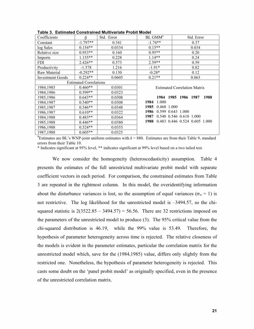
Table 3. Estimated Constrained Multivariate Probit Model Coefficients β Std. Error BL GMMa Std. Error Constant -1.797** 0.341 -1.74** 0.37 log Sales 0.154** 0.0334 0.15** 0.034 Relative size 0.953** 0.160 0.95** 0.20 Imports 1.155** 0.228 1.14** 0.24 FDI 2.426** 0.573 2.59** 0.59 Productivity -1.578 1.216 -1.91* 0.82 Raw Material -0.292** 0.130 -0.28* 0.12 Investment Goods 0.224** 0.0605 0.21** 0.063

Estimated Correlations 1984,1985 0.460** 0.0301 1984,1986 0.599** 0.0323 1985,1986 0.643** 0.0308 1984,1987 0.540** 0.0308 1985,1987 0.546** 0.0348 1986,1987 0.610** 0.0322 1984,1988 0.483** 0.0364 1985,1988 0.446** 0.0380 1986,1988 0.524** 0.0355 1987,1988 0.605** 0.0325

Estimated Correlation Matrix 1984 1985 1986 1987 1988 1984 1.000 1985 0.460 1.000 1986 0.599 0.643 1.000 1987 0.540 0.546 0.610 1.000 1988 0.483 0.446 0.524 0.605 1.000

aEstimates are BL’s WNP-joint uniform estimates with k = 880. Estimates are from their Table 9, standard errors from their Table 10. * Indicates significant at 95% level, ** indicates significant at 99% level based on a two tailed test.

We now consider the homogeneity (heteroscedasticity) assumption. Table 4

presents the estimates of the full unrestricted multivariate probit model with separate

coefficient vectors in each period. For comparison, the constrained estimates from Table

3 are repeated in the rightmost column. In this model, the overidentifying information

about the disturbance variances is lost, so the assumption of equal variances (σtt = 1) is

not restrictive. The log likelihood for the unrestricted model is –3494.57, so the chi-

squared statistic is 2(3522.85 – 3494.57) = 56.56. There are 32 restrictions imposed on

the parameters of the unrestricted model to produce (3). The 95% critical value from the

chi-squared distribution is 46.19, while the 99% value is 53.49. Therefore, the

hypothesis of parameter heterogeneity across time is rejected. The relative closeness of

the models is evident in the parameter estimates, particular the correlation matrix for the

unrestricted model which, save for the (1984,1985) value, differs only slightly from the

restricted one. Nonetheless, the hypothesis of parameter heterogeneity is rejected. This

casts some doubt on the ‘panel probit model’ as originally specified, even in the presence

of the unrestricted correlation matrix.

21

Table 4. Unrestricted Five Period Multivariate Probit Model (Estimated Standard Errors in Parentheses) Coefficients 1984 1985 1986 1987 1988 Constrained Constant -1.802**

(0.532) -2.080** (0.519)

-2.630** (0.542)

-1.721** (0.534)

-1.729** (0.523)

-1.797** (0.341)

log Sales 0.167** (0.0538)

0.178** (0.0565)

0.274** (0.0584)

0.163** (0.0560)

0.130** (0.0519)

0.154** (0.0334)

Relative size 0.658** (0.323)

1.280** (0.330)

1.739** (0.431)

1.085** (0.351)

0.826** (0.263)

0.953** (0.160)

Imports 1.118** (0.377)

0.923** (0.361)

0.936** (0.370)

1.091** (0.338)

1.301** (0.342)

1.155** (0.228)

FDI 2.070** (0.835)

1.509* (0.769)

3.759** (0.990)

3.718** (1.214)

3.834** (1.106)

2.426** (0.573)

Productivity -2.615 (4.110)

-0.252 (3.802)

-5.565 (3.537)

-3.905 (3.188)

-0.981 (2.057)

-1.578 (1.216)

Raw Material -0.346 (0.283)

-0.357 (0.247)

-0.260 (0.299)

0.0261 (0.288)

-0.294 (0.218)

-0.292 (0.130)

Investment Goods

0.239** (0.0864)

0.177* (0.0875)

0.0467 (0.0891)

0.218* (0.0955)

0.280** (0.0923)

0.224** (0.0605)

Estimated Correlation Matrix (Unrestricted shown in bold) 1984 1985 1986 1987 1988 1984 1.000 1985 0.658 0.460 1.000 1986 0.610 0.644 0.599 0.643 1.000 1987 0.548 0.558 0.602 0.540 0.546 0.610 1.000 1988 0.494 0.441 0.537 0.621 0.483 0.446 0.524 0.605 1.000

22

The preceding results suggest that equal parameter vectors in all periods imposes

a substantive restriction on the model. The multivariate probit model with a different

parameter vector in each period relaxes the restriction, but, in practical terms one might

question the nature of that much instability in the underlying structure. Moreover, casual

inspection of Table 4 suggests that the amount of variation across periods is fairly

moderate. The random parameters model lies somewhere between the homogeneous

structure and the multivariate model. They are not nested, as will be seen below; the

heterogeneity in the two models would be interpreted differently. For the multivariate

model, we would view the variation as variation through time of a relationship that is

assumed to be stable across firms. The random parameters model, in contrast, allows for

variation across firms, though at least thus far, we have assumed parameter constancy

through time for each firm. Table 5 presents estimates of the least restrictive form of the

random parameters within the overall structure of this application,

βi = µ + Γwi

where µ and Γ are both unrestricted. (There are no covariates zi, though the industry

segmentation seems like a natural candidate. Since this already appears in the primary

equation, we have not extended the model in this direction.) All parameters were

assumed to be normally distributed across firms.

There are no covariates in the underlying distribution, so the prior means of the

parameter distributions are the elements of µ. Since E[wi] = 0, these are roughly

comparable to the estimated elements of β in the fixed parameter models. Comparing µ

in Table 5 to β in Table 3, we see that there are some substantial differences. Once again

noting the two central parameters, β

ˆ

ˆ

4 and β5 the fixed parameters estimates are 1.155 and

2.426 while the prior means of the random parameters model are 1.582 and 3.111,

respectively. Thus, the impacts implied by the random parameters model are somewhat

greater.

Since wi was modeled as normally distributed for this application, Var[wi] = I.

Thus, the variance of the parameter heterogeneity is Ω = ΓΓ′. The square roots of the

diagonal elements of this matrix are shown in the rightmost column of Table 5. Note,

these are not the sampling standard errors of the estimators, and they are not comparable

23

to the standard errors in the preceding tables. They are the estimated standard deviations

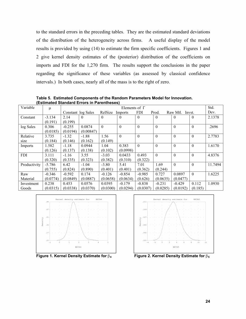
of the distribution of the heterogeneity across firms. A useful display of the model

results is provided by using (14) to estimate the firm specific coefficients. Figures 1 and

2 give kernel density estimates of the (posterior) distribution of the coefficients on

imports and FDI for the 1,270 firm. The results support the conclusions in the paper

regarding the significance of these variables (as assessed by classical confidence

intervals.) In both cases, nearly all of the mass is to the right of zero.

Table 5. Estimated Components of the Random Parameters Model for Innovation. (Estimated Standard Errors in Parentheses)

Variable µ Elements of Γ Constant log Sales RelSize Imports FDI Prod. Raw Mtl. Invst.

Std. Dev.

Constant -3.134 (0.191)

2.14 (0.199)

0 0 0 0 0 0 0 2.1378

log Sales 0.306 (0.0185)

-0.255 (0.0194)

0.0874 (0.00847)

0 0 0 0 0 0 .2696

Relative size

3.735 (0.184)

-1.32 (0.146)

-1.88 (0.162)

1.56 (0.149)

0 0 0 0 0 2.7783

Imports 1.582 (0.126)

-1.18 (0.137)

0.0944 (0.138)

1.04 (0.102)

0.383 (0.0998)

0 0 0 0 1.6170

FDI 3.111 (0.320)

-1.16 (0.335)

3.55 (0.323)

-3.03 (0.382)

0.0433 (0.310)

0.493 (0.322)

0 0 0 4.8376

Productivity -5.786 (0.755)

6.42 (0.824)

-1.04 (0.890)

-3.80 (0.401)

5.41 (0.401)

7.01 (0.362)

1.69 (0.244)

0 0 11.7494

Raw Material

-0.346 (0.0774)

-0.592 (0.0849)

0.174 (0.0887)

-0.126 (0.0658)

-0.854 (0.0634)

-0.985 (0.626)

0.727 (0.0635)

0.0897 (0.0477)

0 1.6225

Investment Goods

0.238 (0.0315)

0.453 (0.0338)

0.0576 (0.0370)

0.0395 (0.0300)

-0.179 (0.0294)

-0.838 (0.0307)

-0.231 (0.0285)

-0.429 (0.0192)

0.112 (0.185)

1.0930

F

Kernel density estimate for BETA4.84

Kernel density estimate for BETA5.211

igure 1. Kernel Density Estimate for β4 F

BETA4

.17

.34

.51

.67

.000 1 2 3 4 5-1

Density

igure 2. Kernel Density Estimate for β5

BETA5

.042

.084

.127

.169

.000-2 0 2 4 6 8 10 12-4

Density

24

The cross period correlation structure implied by the random parameters model is

extremely complicated. In essence, each coefficient contributes its own period specific

random effect, and, moreover, all save that for the constant term are heteroscedastic.

Thus, in practical terms, it is unrestricted. One can reproduce the original model

conveniently by defining period specific dummy variables, dt, and replacing the overall

constant term with random period specific constants. The original model is then

reproduced exactly by constraining the means for the random parameters to be equal.

This gains little over the constrained multivariate model in terms of the structure, but it

gains a large amount in terms of the computational complexity, as it obviates completely

the computation of the T-variate normal probabilities. All that is necessary for estimation

of this form of the model is sampling from the univariate normal distribution. The

parameters of the estimated correlated, equal means random constants model are given in

Table 6. Once again, there are some fairly large differences. Table 6. Estimated Random Effects Model Based on Random Parameters Variable Estimate Standard Error BL Estimate BL Standard Error Constant -3.399** 0.0196 -1.74** 0.37 log Sales 0.284** 0.0181 0.15** 0.034 Relative size 1.550** 0.103 0.95** 0.20 Imports 1.921** 0.129 1.14** 0.24 FDI 4.351** 0.301 2.59** 0.59 Productivity -2.857** 0.557 -1.91* 0.82 Raw Material -0.506** 0.0671 -0.28* 0.12 Investment Goods 0.402** 0.0325 0.21** 0.063

We can deduce the cross period correlation structure from this model as follows.

For this specification of the model, the implied specification is

yit* = β′xit + γt′wi + εit

where β contains the assumed common mean of the random constant terms and γt is row t

of Γ. Therefore, the full T×T disturbance covariance matrix is ΓΓ′ + I. Converting this to

a correlation matrix, we obtained

R =

10.6545 10.6216 0.6468 10.5667 0.5728 0.5546 10.5020 0.4461 0.5020 0.6206 1

25

which is quite close to the results given in Tables 3 and 4.

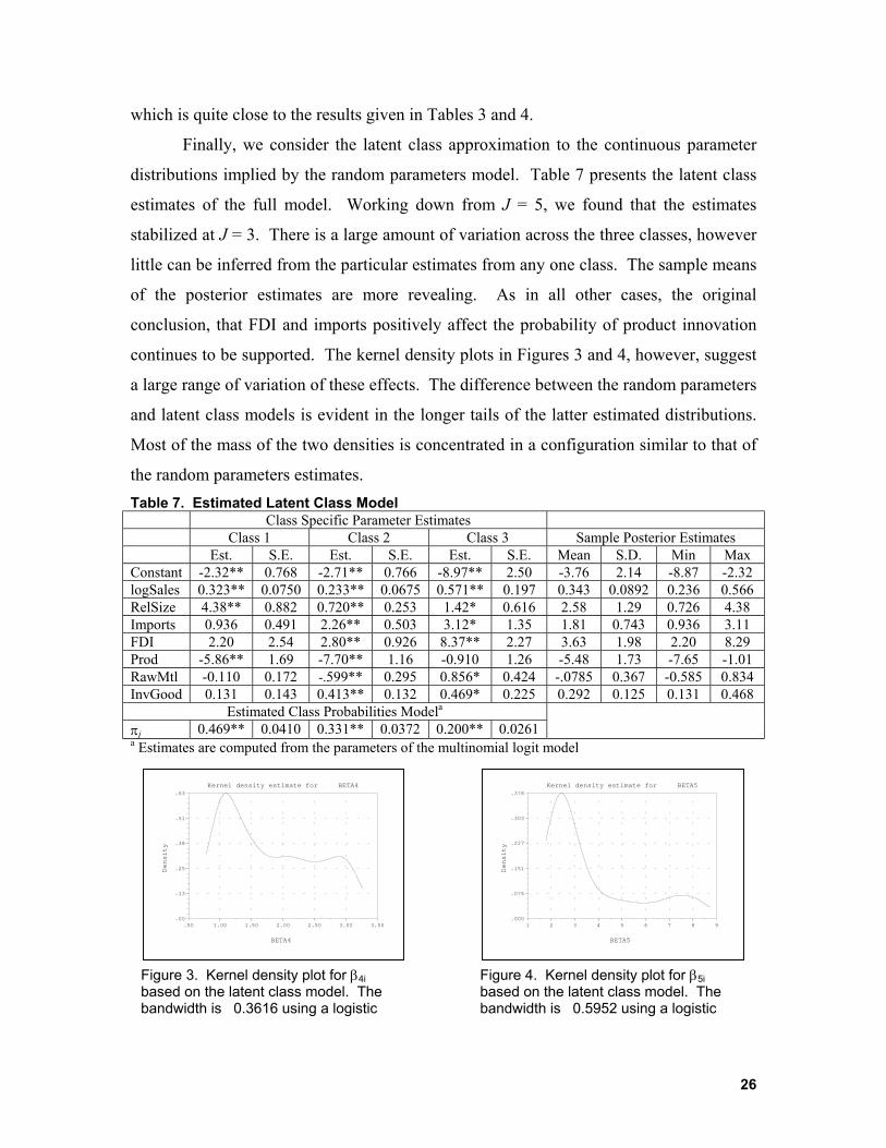
Finally, we consider the latent class approximation to the continuous parameter

distributions implied by the random parameters model. Table 7 presents the latent class

estimates of the full model. Working down from J = 5, we found that the estimates

stabilized at J = 3. There is a large amount of variation across the three classes, however

little can be inferred from the particular estimates from any one class. The sample means

of the posterior estimates are more revealing. As in all other cases, the original

conclusion, that FDI and imports positively affect the probability of product innovation

continues to be supported. The kernel density plots in Figures 3 and 4, however, suggest

a large range of variation of these effects. The difference between the random parameters

and latent class models is evident in the longer tails of the latter estimated distributions.

Most of the mass of the two densities is concentrated in a configuration similar to that of

the random parameters estimates. Table 7. Estimated Latent Class Model Class Specific Parameter Estimates Class 1 Class 2 Class 3 Sample Posterior Estimates Est. S.E. Est. S.E. Est. S.E. Mean S.D. Min Max Constant -2.32** 0.768 -2.71** 0.766 -8.97** 2.50 -3.76 2.14 -8.87 -2.32 logSales 0.323** 0.0750 0.233** 0.0675 0.571** 0.197 0.343 0.0892 0.236 0.566 RelSize 4.38** 0.882 0.720** 0.253 1.42* 0.616 2.58 1.29 0.726 4.38 Imports 0.936 0.491 2.26** 0.503 3.12* 1.35 1.81 0.743 0.936 3.11 FDI 2.20 2.54 2.80** 0.926 8.37** 2.27 3.63 1.98 2.20 8.29 Prod -5.86** 1.69 -7.70** 1.16 -0.910 1.26 -5.48 1.73 -7.65 -1.01 RawMtl -0.110 0.172 -.599** 0.295 0.856* 0.424 -.0785 0.367 -0.585 0.834 InvGood 0.131 0.143 0.413** 0.132 0.469* 0.225 0.292 0.125 0.131 0.468

Estimated Class Probabilities Modela

πj 0.469** 0.0410 0.331** 0.0372 0.200** 0.0261

a Estimates are computed from the parameters of the multinomial logit model

Kernel density estimate for BETA4

BETA4

.13

.25

.38

.51

.63

.001.00 1.50 2.00 2.50 3.00 3.50.50

Density

Kernel density estimate for BETA5

BETA5

.076

.151

.227

.303

.378

.0002 3 4 5 6 7 8 91

Density

Figure 3. Kernel density plot for β4i based on the latent class model. Thebandwidth is 0.3616 using a logistic k l

Figure 4. Kernel density plot for β5i based on the latent class model. Thebandwidth is 0.5952 using a logistic k l

26

5. Conclusions

The preceding has examined a number of estimators for the panel probit model.

The GMM estimator appears to perform fairly well compared to the maximum likelihood

estimator. On the other hand, the difficulty of obtaining the latter is considerably smaller

than the discussion in BL would suggest. Part of this stems from the much greater speeds

attainable with the current vintage of computers. However, it also appears that the

authors were unduly pessimistic about the feasibility of using simulation methods for

computation of the multivariate normal integrals needed for FIML estimation.

Obviously, it is unclear what sample sizes should be used as the benchmarks for this

discussion. However, their application, with N = 1,270, K = 8 and T = 5, is reasonably

large enough that one should be able to obtain some guidance from our results.

We also presented two alternative models for the panel based discrete choice

analysis. These are not simple alternatives to the panel probit model suggested by BL.

The random parameters model and latent class model are more elaborate model

specifications that allow the analyst to glean from a rich panel such as this one

information about individual heterogeneity that is neglected by the simple model

formulation suggested by BL. The computation of the latent class model is exceedingly

simple. Computation of the model reported here took less than 30 seconds. The random

parameters model is much more computationally intensive as it requires maximization of

a simulated log likelihood function. Nonetheless, with the use of a quasi Monte Carlo

method, specifically Halton sequences as an alternative to simulated random sampling,

estimation of the model is not unduly burdensome..

Appendix. Quasi Monte Carlo Integration Gourieroux and Monfort (1996) provide the essential statistical background for

the simulated maximum likelihood estimator. We assume that the original maximum

likelihood estimator as posed with the intractable integral is otherwise regular - if

computable, the MLE would have the familiar properties, consistency, asymptotic

normality, asymptotic efficiency, and invariance to smooth transformation. Let θ denote

the full vector of unknown parameters being estimated and let qML denote the maximum

likelihood estimator of the full parameter vector shown above, and let qSML denote the

27

simulated maximum likelihood (SML) estimator. Gourieroux and Monfort establish that

if N /R → 0 and R and N → ∞, then N (qSML - θ) has the same limiting normal

distribution with zero mean as N (qML - θ). That is, under the assumptions, the

maximum simulated likelihood estimator and the true maximum likelihood estimator are

asymptotically equivalent. The requirement that the number of draws, R, increase faster

than the square root of the number of observations, N, is important to their result. The

requirement is easily met by tying R to the sample size, as in, for example, R = N.5+δ for

some positive δ. There does remain a finite R bias in the estimator, which the authors

obtain as approximately equal to (1/R) times a vector which is a finite vector of constants

(see p. 44). Generalities are difficult, but the authors suggest that when the MLE is

relatively "precise," the bias is likely to be small. In Munkin and Trivedi's (2000) Monte

Carlo study of the effect, in samples of 1000 and numbers of replications around 200 or

300, the bias of the simulation based estimator appears to be trivial.

The results thus far are based on random sampling from the underlying

distribution of w. But, the simulation method, itself, contributes to the variation of SML

estimator. [See, e.g., Geweke (1995).] Judicious choice of the random draws for the

simulation can be helpful in speeding up the convergence. [See Bhat (1999).] One

technique commonly used is antithetic sampling. [See Geweke (1995, 1998) and Ripley

(1987).] The technique involves sampling R/2 independent pairs of draws where the

members of the pair are negatively correlated. One technique often used, for example is

to pair each draw wir with -wir. (A loose end in the discussion at this point concerns what

becomes of the finite simulation bias in the estimator. The results in Gourieroux and

Monfort hinge on random sampling.)

Quasi Monte Carlo (QMC) methods are based on replacing the pseudo random

draws of the Monte Carlo integration with a grid of "cleverly" selected points which are

nonrandom but provide more uniform coverage of the domain of the integral. The logic

of the technique is that randomness of the draws used in the integral is not the objective

in the calculation. Convergence of the average to the expectation (integral) is, and this

can be achieved by other types of sequences. A number of such strategies is surveyed in

Bhat (1999), Sloan and Wozniakowski (1998) and Morokoff and Caflisch (1995). The

advantage of QMC as opposed to MC integration is that for some types of sequences, the

28

accuracy is far greater, convergence is much faster and the simulation variance is smaller.

For the one we will advocate here, Halton sequences, Bhat (1995) found relative

efficiencies of the QMC method to the MC method in moderately sized estimation

problems to be on the order of ten or twenty to one.

Monte Carlo simulation based estimation uses a random number generator to

produce the draws from a specified distribution. The central component of the approach

is draws from the standard continuous uniform distribution, U[0,1]. Draws from other

distributions are obtained from these by using the inverse probability transformation. In

particular, if ui is one draw from U[0,1], then vi = Φ-1(ui) produces a draw from the

standard normal distribution; vi can then be unstandardized by the further transformation

zi = σvi + µ. Draws from other distributions used, e.g., in Train (1999) are the uniform

[-1,1] distribution for which vi = 2ui-1 and the tent distribution, for which vi = 12 −iu

if ui ≤ 0.5, vi = 1 - 12 −iu otherwise. Geweke (1995), and Geweke, Hajivassiliou, and

Keane (1994) discuss simulation from the multivariate truncated normal distribution with

this method.

The Halton sequence is generated as follows: Let r be a prime number larger than

2. Expand the sequence of integers g = 1,... in terms of the base r as

where by construction, 0 ≤ bi

iIi

rbg ∑ ==

0 i ≤ r - 1 and rI ≤ g < rI+1. The Halton sequence of values that corresponds to this series is 1

0)( −−=∑= i

iIir rbgH

For example, using base 5, the integer 37 has b0 = 2, b1 = 2, and b3 = 1. Then

H5(37) = 2×5-1 + 2×5-2 + 1×5-3 = 0.448. The sequence of Halton values is efficiently spread over the unit interval. The sequence

is not random as the sequence of pseudo-random numbers is. Figures 5 and 6 below

show two sequences of 1,000 Halton draws based on r = 7 and r = 9 and two sequences

of 1,000 psuedorandom draws. The clumping evident in the figure on the left is the

feature that necessitates large pseudo-samples for simulations.

29

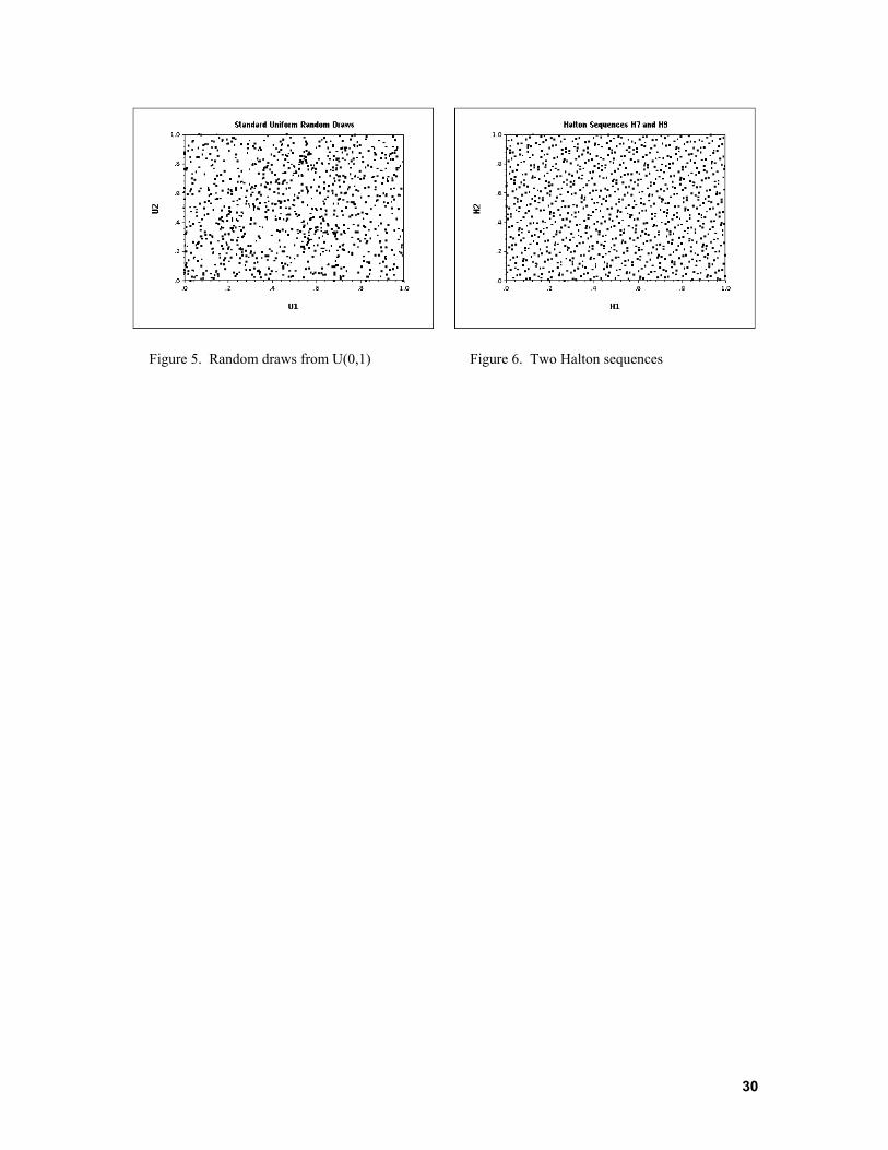
Figure 5. Random draws from U(0,1) Figure 6. Two Halton sequences

30

References Ahn, S. and P. Schmidt, "Efficient Estimation of Models for Dynamic Panel Data," Journal of

Econometrics, 68, 1995, pp. 3-38. Akin, J., D. Guilkey and R. Sickles, A Random Coefficient Probit Model with an Application to a Study of

Migration," Journal of Econometrics, 11, 1979, pp. 233-246. Arellano, M. and O. Bover, "Another Look at the Instrumental Variable Estimation of Error-Components

Models," Journal of Econometrics, 68, 1995, pp. 29-51. Avery, R., L. Hansen and J. Hotz, “Multiperiod Probit Models and Orthogonality Condition Estimation,”

International Economic Review, 24, 1983, pp. 21-35. Bertschek, I., “Product and Process Innovation as a Response to increasing Imports and Foreign Direct

Investment, Journal of Industrial Economics, 43, 4, 1995, pp. 341-357. Bertschek, I. and M. Lechner, “Convenient Estimators for the Panel Probit Model,” Journal of

Econometrics, 87,2, 1998, pp. 329-372. Bhat, C., "Quasi-Random Maximum Simulated Likelihood Estimation of the Mixed Multinomial Logit

Model," Manuscript, Department of Civil Engineering, University of Texas, Austin, 1999. Boyes, W., Hoffman, D. and S. Low, “An Econometric Analysis of the Bank Credit Scoring Problem,”

Journal of Econometrics, 40, 1989, pp. 3-14. Brannas, K. and G. Rosenqvist, "Semiparametric Estimation of Heterogeneous Count Data Models,"

European Journal of Operational Research, 76, 1994, pp. 247-258. Breitung, J. and M. Lechner, “GMM Estimation of Nonlinear Models on Panel Data,” Humboldt

University, SFB, Discussion paper, 67, 1995; “Estimation de modeles non lineaires, sur donnees de panel par la methode des moments generalises,” Economie et Prevision, 1997.

Burnett, N., “Gender Economics Courses in Liberal Arts Colleges,” Journal of Economic Education, 24, 8, 1997, pp. 369-377.

Butler, J. and R. Moffitt, "A Computationally Efficient Quadrature Procedure for the One Factor Multinomial Probit Model," Econometrica, 50, 1982, pp. 761-764.

Dempster, A., N. Laird and D. Rubin, "Maximum Likelihood From Incomplete Data via the E.M. Algorithm," Journal of the Royal Statistical Society, Series B, 39, 1, 1977, pp. 1-38.

Geweke, J., "Monte Carlo Simulation and Numerical Integration," Staff Research Report 192, Federal Reserve Bank of Minneapolis, 1995.

Geweke, J., "Posterior Simulators in Econometrics," in Kreps, D. and K. Wallis, eds., Advances in Statistics and Econometrics: Theory and Applications, Vol III, Cambridge University Press, Cambridge, 1997.

Geweke, J., M. Keane and D. Runkle, "Alternative Computational Approaches to Inference in the Multinomial Probit Model," Review of Economics and Statistics, 76, 1994, pp. 609-632.

Geweke, J., M. Keane and D. Runkle, "Statistical Inference in the Multinomial Multiperiod Probit Model," Journal of Econometrics, 81, 1, 1997, pp. 125-166.

Gourieroux, C. and A. Monfort, Simulation Based Econometrics, Oxford University Press, New York, 1996.

Greene, W., "A Statistical Model for Credit Scoring," Stern School of Business, Dept. of Economics, Working paper # 92-10, 1992.

Greene, W., “Gender Economics Courses in Liberal Arts Colleges: Further Results,” Journal of Economic Education, fall, 1998, pp. 291-300.

Greene, W., “Fixed and Random Effects in Nonlinear Models,” Working Paper 01-10, Department of Economics, Stern School of Business, (http://www.stern.nyu.edu/~wgreene/panel.pdf), 2001.

Greene, W., The Behavior of the Fixed Effects Estimator in Nonlinear Models, Stern School of Business, New York University, Department of Economics, Working Paper 02-03, (http://www.stern.nyu.edu/~wgreene/nonlinearfixedeffects.pdf), 2002

Greene, W., Econometric Analysis, 5th ed., Prentice Hall, Englewood Cliffs, 2003. (forthcoming) Guilkey, D., and J. Murphy, "Estimation and Testing in the Random Effects Probit Model," Journal of

Econometrics, 59, 1993, pp. 301-317. Hajivassiliou, V., D. McFadden and P. Ruud, “Simulation of Multivariate Normal Orthatn Probabilities:

Methods and Programs,” Journal of Eeconometrics, 72, 1996, pp. 85-134. Hajivassiliou, V. and P. Ruud, "Classical Estimation Methods for LDV Models Using Simulation," In

Engle, R. and D. McFadden, eds., Handbook of Econometrics, Vol. IV, North Holland, Amsterdam, 1994.

31

Hansen, L. “Large Sample Properties of Generalized Method of Moments Estimators,” Econometrica, 50, 1982, pp. 1029-1054.

Heckman, J. 1981. The incidental parameters problem and the problem of initial conditions in estimating a discrete time-discrete data stochastic process. In Structural Analysis of Discrete Data with Econometric Applications, Manski, C. and McFadden D. (eds). MIT Press: Cambridge.

L'Ecuyer, P, "Good Parameters and Implementations for Combined Multiple Recursive Random Number Generators," Department of Information Science, University of Montreal, working paper, 1998.

McFadden, D. and K. Train, "Mixed MNL Models for Discrete Response," Journal of Applied Econometrics, 15, 2000, pp. 447-470.

McLachlan, G. and D. Peel, Finite Mixture Models, New York, John Wiley and Sons, 2000. Morokoff, W., and R. Calflisch, "Quasi-Monte Carlo Integration," Journal of Computational Physics, 122,

1995, pp. 218-230. Munkin, M. and P. Trivedi, "Econometric Analysis of a Self Selection Model with Multiple Outcomes

Using Simulation-Based Estimation: An Application to the Demand for Healthcare," Manuscript, Department of Economics, Indiana University, 2000.

Nagin, D. and K. Land, "Age, Criminal Careers, and Population Heterogeneity: Specification and Estimation of a Nonparametric, Mixed Poisson Model," Criminology, 31, 3, 1993, pp. 327-362.

Ripley, B., Stochastic Simulation, John Wiley and Sons, New York, 1987. Rubinfeld, D., “Voting in a Local School Election: A Micro Analysis,” Review of Economics and Statistics,

59, 1983, 30-42. Sepanski, J., "On a Random Coefficient Probit Model," Communications in Statistics - Theory and

Methods, 29, 11, 2000, pp. 2493-2505. Sloan, J. and H. Wozniakowski, "When are Quasi-Monte Carlo Algorithms Efficient for High Dimensional

Integrals," Journal of Complexity, 14, 1998, pp. 1-33. Stata Corp, Stata Statistical Software: Release 6.0, College Station, TX, Stata Corp., 1998. Train, K., "Halton Sequences for Mixed Logit," Manuscript, Department of Economics, University of

California, Berkeley, 1999. Train, K., Discrete Choice Methods with Simulation, Cambridge University Press, Cambridge, 2002. Wang, P., I. Cockburn, and M. Puterman, "Analysis of Patent Data - A Mixed Poisson Regression Model

Approach," Journal of Business and Economic Statistics, 16, 1, 1998, pp. 27-41. Wedel, M., W. DeSarbo, J. Bult, and V. Ramaswamy, "A Latent Class Poisson Regression Model for

Heterogeneous Count Data," Journal of Applied Econometrics, 8, 1993, pp. 397-411. White, H., “Maximum Likelihood Estimation of Misspecified Models,” Econometrica, 50, 1982, pp. 1-25. Wooldridge, J., "Selection Corrections for Panel Data Models Under Conditional Mean Independence

Assumptions," Journal of Econometrics, 68, 1995, pp. 115-132.

32