conventions used in erdas imagine, the names of menus, … · 2018-05-08 · map composer open the...
TRANSCRIPT
xiv Conventions Used in This Book
Conventions Used in This Book
In ERDAS IMAGINE, the names of menus, menu options, buttons, and other components of the interface are shown in bold type. For example:
“In the Select Layer To Add dialog, select the Fit to Frame option.”
When asked to use the mouse, you are directed to click, Shift-click, middle-click, right-click, hold, drag, etc.
• click—designates clicking with the left mouse button.
• Shift-click—designates holding the Shift key down on your keyboard and simultaneously clicking with the left mouse button.
• middle-click—designates clicking with the middle mouse button.
• right-click—designates clicking with the right mouse button.
• hold—designates holding down the left (or right, as noted) mouse button.
• drag—designates dragging the mouse while holding down the left mouse button.
The following paragraphs are used throughout the ERDAS IMAGINE documentation:
These paragraphs contain strong warnings.
These paragraphs provide software-specific information.
These paragraphs contain important tips.
These paragraphs lead you to other areas of this book or other ERDAS® manuals for additional information.
NOTE: Notes give additional instruction.
Shaded BoxesShaded boxes contain supplemental information that is not required to execute the steps of a tour guide, but is noteworthy. Generally, this is technical information.

xvGetting Started
Getting Started To start ERDAS IMAGINE, type the following in a UNIX command window: imagine, or select ERDAS IMAGINE from the Start menu.
ERDAS IMAGINE begins running; the icon panel automatically opens.
ERDAS IMAGINE Icon Panel
The ERDAS IMAGINE icon panel contains icons and menus for accessing ERDAS IMAGINE functions. You have the option (through the Session -> Preferences menu) to display the icon panel horizontally across the top of the screen or vertically down the left side of the screen. The default is a horizontal display.
The icon panel that displays on your screen looks similar to the following:
The various icons that are present on your icon panel depend on the components and add-on modules you have purchased with your system.
ERDAS IMAGINE Menu Bar
The menus on the ERDAS IMAGINE menu bar are: Session, Main, Tools, Utilities, and Help. These menus are described in this section.
NOTE: Any items which are unavailable in these menus are shaded and inactive.
Session Menu
1. Click the word Session in the upper left corner of the ERDAS IMAGINE menu bar. The Session menu opens:
Click here to end the ERDAS IMAGINE You can also place the
cursor anywhere in the icon panel and press Ctrl-Q to exit ERDAS
These menus are identical to the ones on the icon panel.
session
IMAGINE
xvi Getting Started
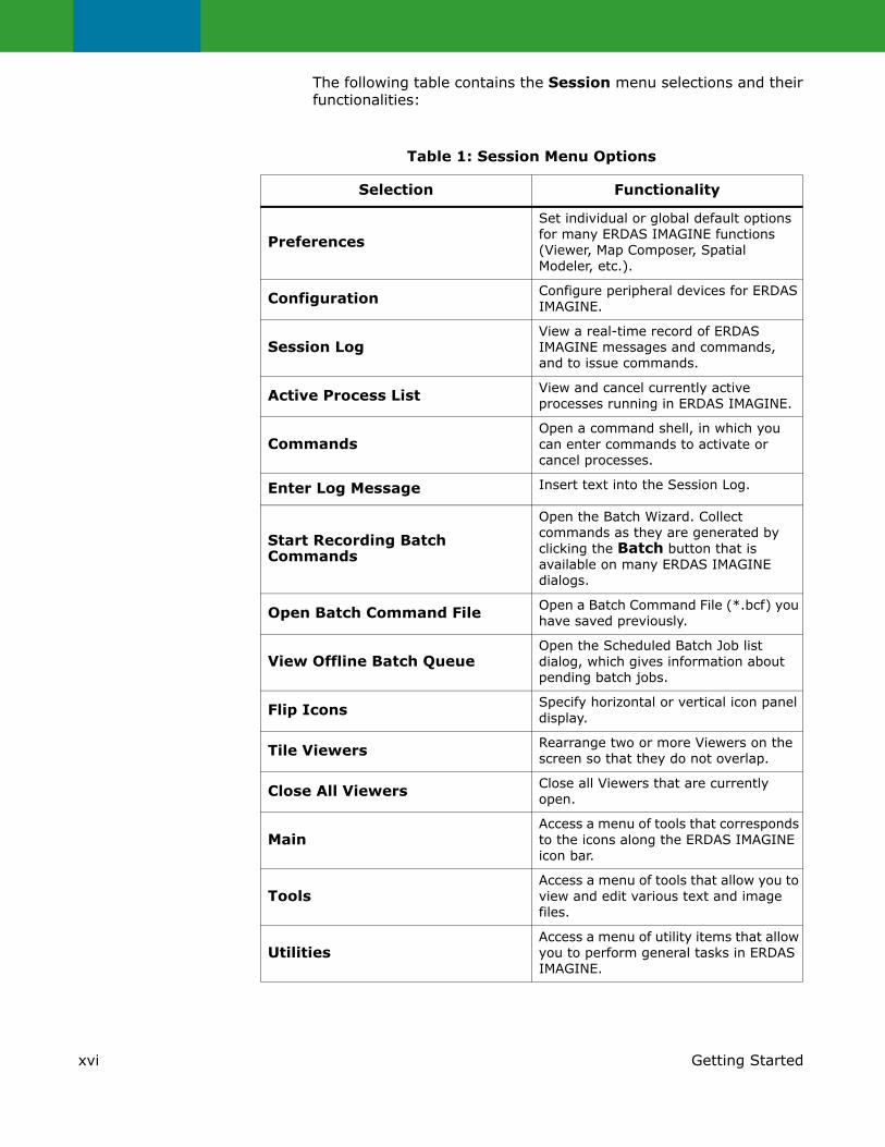
The following table contains the Session menu selections and their functionalities:
Table 1: Session Menu Options
Selection Functionality
Preferences
Set individual or global default options for many ERDAS IMAGINE functions (Viewer, Map Composer, Spatial Modeler, etc.).
Configuration Configure peripheral devices for ERDAS IMAGINE.
Session LogView a real-time record of ERDAS IMAGINE messages and commands, and to issue commands.
Active Process List View and cancel currently active processes running in ERDAS IMAGINE.
CommandsOpen a command shell, in which you can enter commands to activate or cancel processes.
Enter Log Message Insert text into the Session Log.
Start Recording Batch Commands
Open the Batch Wizard. Collect commands as they are generated by clicking the Batch button that is available on many ERDAS IMAGINE dialogs.
Open Batch Command File Open a Batch Command File (*.bcf) you have saved previously.
View Offline Batch QueueOpen the Scheduled Batch Job list dialog, which gives information about pending batch jobs.
Flip Icons Specify horizontal or vertical icon panel display.
Tile Viewers Rearrange two or more Viewers on the screen so that they do not overlap.
Close All Viewers Close all Viewers that are currently open.
MainAccess a menu of tools that corresponds to the icons along the ERDAS IMAGINE icon bar.
ToolsAccess a menu of tools that allow you to view and edit various text and image files.
UtilitiesAccess a menu of utility items that allow you to perform general tasks in ERDAS IMAGINE.
xviiGetting Started
Main Menu
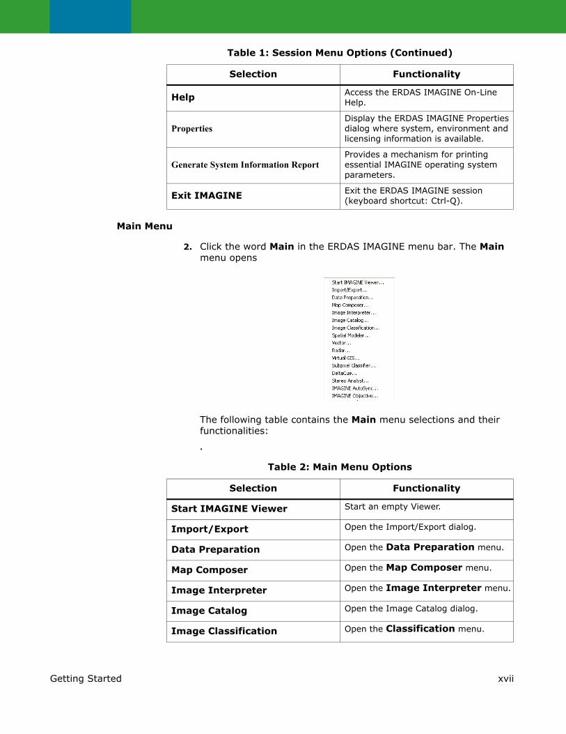
2. Click the word Main in the ERDAS IMAGINE menu bar. The Main menu opens
The following table contains the Main menu selections and their functionalities:
.
Help Access the ERDAS IMAGINE On-Line Help.
PropertiesDisplay the ERDAS IMAGINE Properties dialog where system, environment and licensing information is available.
Generate System Information ReportProvides a mechanism for printing essential IMAGINE operating system parameters.
Exit IMAGINE Exit the ERDAS IMAGINE session (keyboard shortcut: Ctrl-Q).
Table 1: Session Menu Options (Continued)
Selection Functionality
Table 2: Main Menu Options
Selection Functionality
Start IMAGINE Viewer Start an empty Viewer.
Import/Export Open the Import/Export dialog.
Data Preparation Open the Data Preparation menu.
Map Composer Open the Map Composer menu.
Image Interpreter Open the Image Interpreter menu.
Image Catalog Open the Image Catalog dialog.
Image Classification Open the Classification menu.

xviii Getting Started
Tools Menu
3. Click the word Tools in the ERDAS IMAGINE menu bar. The Tools menu opens:
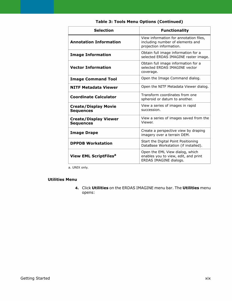
The following table contains the Tools menu selections and their functionalities:
Spatial Modeler Open the Spatial Modeler menu.
Vector Open the Vector Utilities menu.
Radar Open the Radar menu.
VirtualGIS Open the VirtualGIS menu.
Subpixel Classifier Open the Subpixel menu.
DeltaCue Open the DeltaCue menu.
Stereo Analyst Open the Stereo Analyst Workspace.
IMAGINE AutoSync Open the AutoSync menu.
IMAGINE Objective Open the Objective menu.
Table 2: Main Menu Options (Continued)
Selection Functionality
Table 3: Tools Menu Options
Selection Functionality
Edit Text Files Create and edit ASCII text files.
Edit Raster Attributes Edit raster attribute data.
View Binary Data View the contents of binary files in a number of different ways.
View IMAGINE HFA File Structure
View the contents of the ERDAS IMAGINE hierarchical files.
xixGetting Started
Utilities Menu
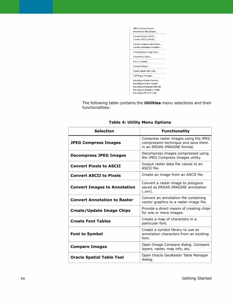
4. Click Utilities on the ERDAS IMAGINE menu bar. The Utilities menu opens:
Annotation InformationView information for annotation files, including number of elements and projection information.
Image Information Obtain full image information for a selected ERDAS IMAGINE raster image.
Vector InformationObtain full image information for a selected ERDAS IMAGINE vector coverage.
Image Command Tool Open the Image Command dialog.
NITF Metadata Viewer Open the NITF Metadata Viewer dialog.
Coordinate Calculator Transform coordinates from one spheroid or datum to another.
Create/Display Movie Sequences
View a series of images in rapid succession.
Create/Display Viewer Sequences
View a series of images saved from the Viewer.
Image Drape Create a perspective view by draping imagery over a terrain DEM.
DPPDB Workstation Start the Digital Point Positioning DataBase Workstation (if installed).
View EML ScriptFilesaOpen the EML View dialog, which enables you to view, edit, and print ERDAS IMAGINE dialogs.
a. UNIX only.
Table 3: Tools Menu Options (Continued)
Selection Functionality
xx Getting Started
The following table contains the Utilities menu selections and their functionalities:
Table 4: Utility Menu Options
Selection Functionality
JPEG Compress ImagesCompress raster images using the JPEG compression technique and save them in an ERDAS IMAGINE format.
Decompress JPEG Images Decompress images compressed using the JPEG Compress Images utility.
Convert Pixels to ASCII Output raster data file values to an ASCII file.
Convert ASCII to Pixels Create an image from an ASCII file.
Convert Images to AnnotationConvert a raster image to polygons saved as ERDAS IMAGINE annotation (.ovr).
Convert Annotation to Raster Convert an annotation file containing vector graphics to a raster image file.
Create/Update Image Chips Provide a direct means of creating chips for one or more images.
Create Font Tables Create a map of characters in a particular font.
Font to SymbolCreate a symbol library to use as annotation characters from an existing font.
Compare Images Open Image Compare dialog. Compare layers, raster, map info, etc.
Oracle Spatial Table Tool Open Oracle GeoRaster Table Manager dialog.
xxiGetting Started
Help Menu
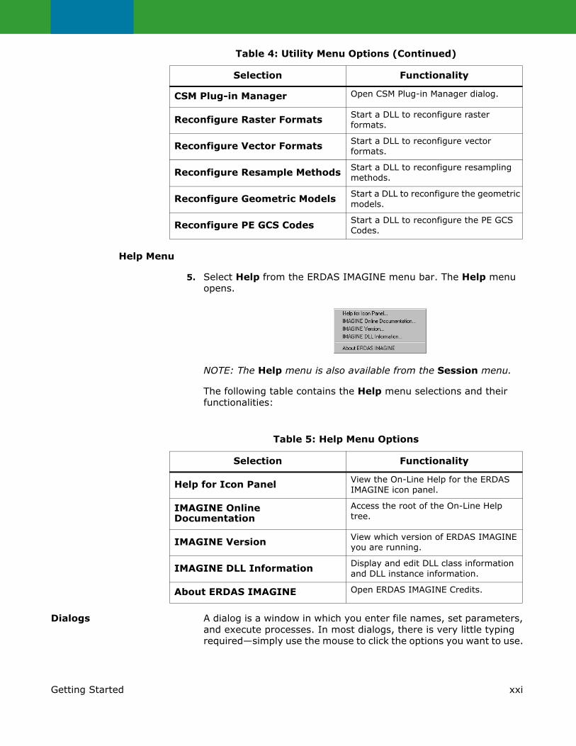
5. Select Help from the ERDAS IMAGINE menu bar. The Help menu opens.
NOTE: The Help menu is also available from the Session menu.
The following table contains the Help menu selections and their functionalities:
Dialogs A dialog is a window in which you enter file names, set parameters, and execute processes. In most dialogs, there is very little typing required—simply use the mouse to click the options you want to use.
CSM Plug-in Manager Open CSM Plug-in Manager dialog.
Reconfigure Raster Formats Start a DLL to reconfigure raster formats.
Reconfigure Vector Formats Start a DLL to reconfigure vector formats.
Reconfigure Resample Methods Start a DLL to reconfigure resampling methods.
Reconfigure Geometric Models Start a DLL to reconfigure the geometric models.
Reconfigure PE GCS Codes Start a DLL to reconfigure the PE GCS Codes.
Table 4: Utility Menu Options (Continued)
Selection Functionality
Table 5: Help Menu Options
Selection Functionality
Help for Icon Panel View the On-Line Help for the ERDAS IMAGINE icon panel.
IMAGINE Online Documentation
Access the root of the On-Line Help tree.
IMAGINE Version View which version of ERDAS IMAGINE you are running.
IMAGINE DLL Information Display and edit DLL class information and DLL instance information.
About ERDAS IMAGINE Open ERDAS IMAGINE Credits.
xxii More Information/Help
Most of the dialogs used throughout the tour guides are reproduced from the software, with arrows showing you where to click. These instructions are for reference only. Follow the numbered steps to actually select dialog options.
For On-Line Help with a particular dialog, click the Help button in that dialog.
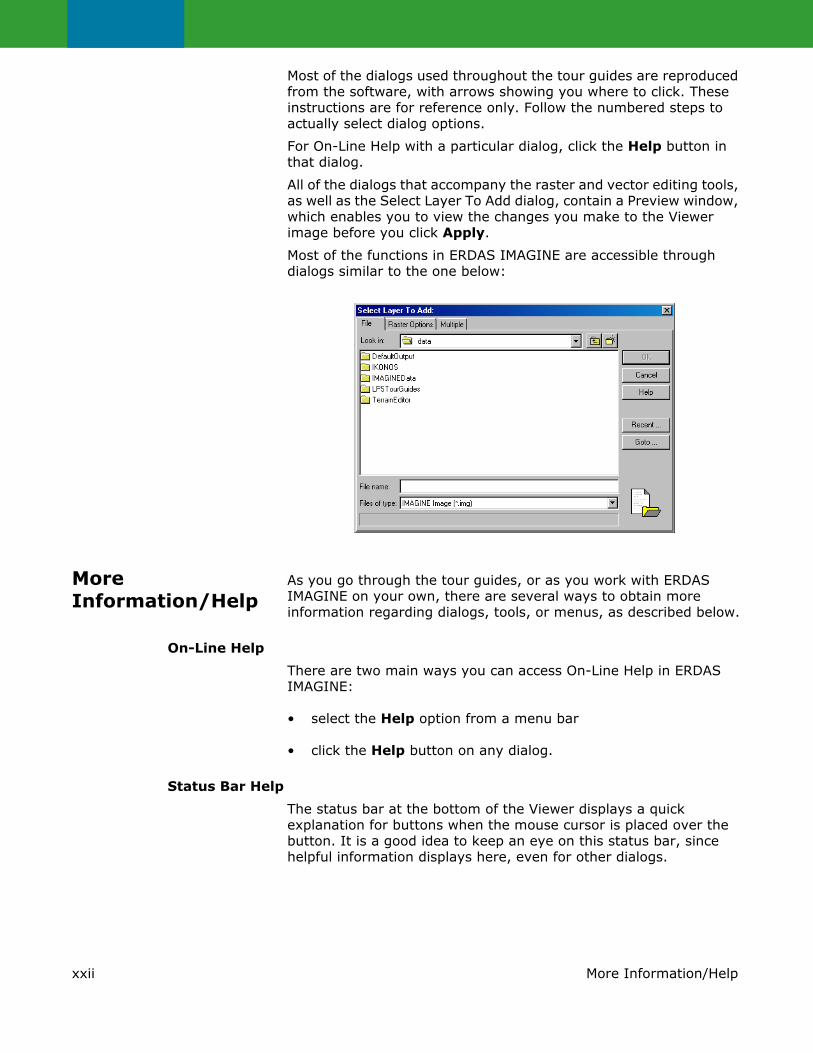
All of the dialogs that accompany the raster and vector editing tools, as well as the Select Layer To Add dialog, contain a Preview window, which enables you to view the changes you make to the Viewer image before you click Apply.
Most of the functions in ERDAS IMAGINE are accessible through dialogs similar to the one below:
More Information/Help
As you go through the tour guides, or as you work with ERDAS IMAGINE on your own, there are several ways to obtain more information regarding dialogs, tools, or menus, as described below.
On-Line Help
There are two main ways you can access On-Line Help in ERDAS IMAGINE:
• select the Help option from a menu bar
• click the Help button on any dialog.
Status Bar Help
The status bar at the bottom of the Viewer displays a quick explanation for buttons when the mouse cursor is placed over the button. It is a good idea to keep an eye on this status bar, since helpful information displays here, even for other dialogs.

xxiiiMore Information/Help
Bubble Help
The User Interface and Session category of the Preference Editor enables you to turn on Bubble Help, so that the single-line Help displays directly below your cursor when your cursor rests on a button or frame part. This is helpful if the status bar is obscured by other windows.

xxiv More Information/Help

1Display Preferences
Viewer & Geospatial Light Table
Introduction In this tour guide, you can learn how to:
• set Preferences
• display an image
• query for pixel information
• arrange layers
• adjust image contrast
• link Viewers
• use the Area of Interest (AOI) function
• use the Raster menu functions (Raster Attribute Editor, Measurement tools, and so on)
• use the geospatial light table
Approximate completion time for this tour guide is 45 minutes.
Display Preferences
ERDAS IMAGINE allows you to set up default band-to-color gun assignments for Landsat MSS, Landsat TM, SPOT, and AVHRR data in the Preference Editor.
Check Band-to-Color Gun Assignments
ERDAS IMAGINE should be running and a Viewer should be open.
1. Click the word Session in the upper left corner of the ERDAS IMAGINE menu bar.
2. From the Session menu, click Preferences.
The Preference Editor opens.

2 Display Preferences
3. Drag the scroll bar on the right side of the dialog down to see all of the User Interface & Session preferences (User Interface & Session is the default under Category).
You may change these or any other preferences at any time by selecting the preference category (click the list below Category) and then editing the text in the text entry fields.
4. Under the User Interface & Session category in the Preference Editor, locate the preferences for the 3-Band Image Red Channel default, 3-Band Image Green Channel default, 3-Band Image BlueChannel default, 4-Band Image Red Channel default, 4-Band Image Green Channel default, 4-Band Image Blue Channel Default, 5-Band Image Red Channel default, 5-Band Image Green Channel default, 5-Band Image Blue Channel Default, 6-or-greater-Band Image Red Channel default, 6-or-greater-Band Image Green Channel default, and 6-or-greater-Band Image Blue Channel Defaults.
The number that is entered for these defaults shows the band that is used for the Red, Green, and Blue color guns in your display. You may change these defaults. These are the band assignments that display in the Layers to Colors section of the Select Layer To Add dialog when it opens. These assignments can also be changed in the Select Layer To Add dialog for specific files.
Check Viewer Preferences
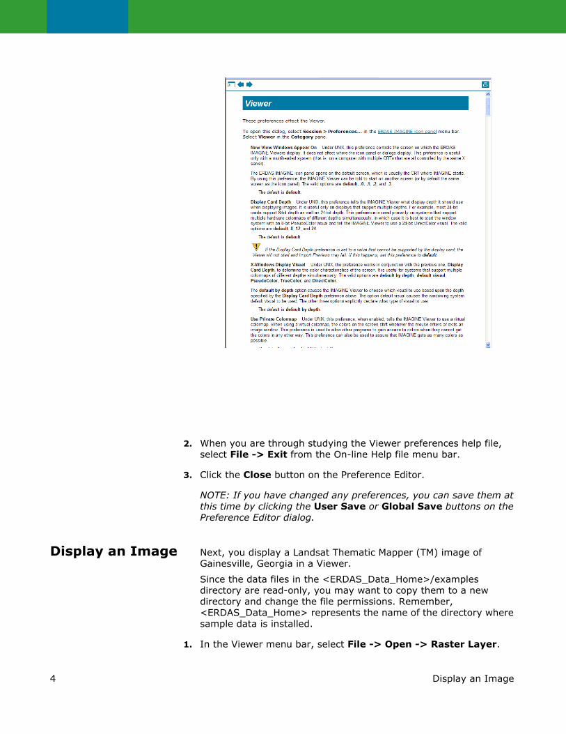
1. With the Preference Editor still open, click the Category list and select Viewer.
The Viewer preferences display.
2. Drag the scroll bar on the right of the dialog down to see all of the Viewer preferences.
These preferences control the way the Viewer automatically displays and responds each time it opens.
Click hereto see on-linehelp for thisdialog
Click here to select thepreference
Click hereto see on-linehelp for thiscategory
categories
3Display Preferences
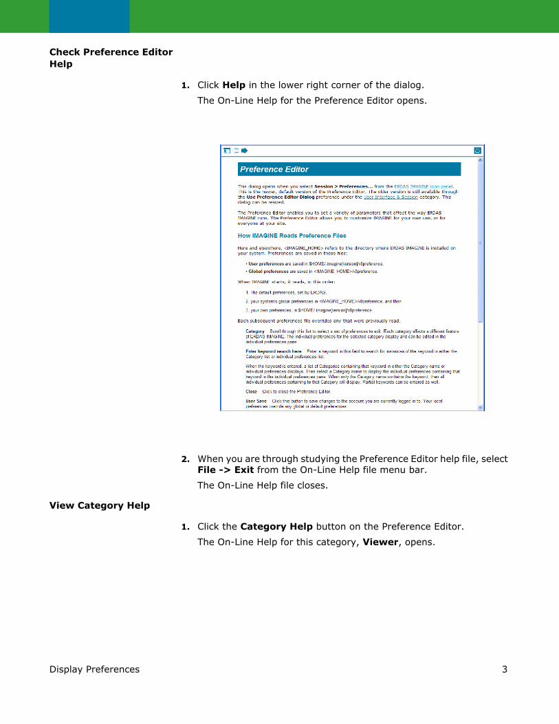
Check Preference Editor Help
1. Click Help in the lower right corner of the dialog.
The On-Line Help for the Preference Editor opens.
2. When you are through studying the Preference Editor help file, select File -> Exit from the On-Line Help file menu bar.
The On-Line Help file closes.
View Category Help
1. Click the Category Help button on the Preference Editor.
The On-Line Help for this category, Viewer, opens.
4 Display an Image
2. When you are through studying the Viewer preferences help file, select File -> Exit from the On-line Help file menu bar.
3. Click the Close button on the Preference Editor.
NOTE: If you have changed any preferences, you can save them at this time by clicking the User Save or Global Save buttons on the Preference Editor dialog.
Display an Image Next, you display a Landsat Thematic Mapper (TM) image of Gainesville, Georgia in a Viewer.
Since the data files in the <ERDAS_Data_Home>/examples directory are read-only, you may want to copy them to a new directory and change the file permissions. Remember, <ERDAS_Data_Home> represents the name of the directory where sample data is installed.
1. In the Viewer menu bar, select File -> Open -> Raster Layer.

5Display an Image
You can also open this dialog using either of these two methods:
— use the keyboard shortcut, Ctrl-r
— click this icon in the Viewer toolbar.
The Select Layer To Add dialog opens.
2. In the Select Layer To Add dialog, click the Recent button.
A dialog with a listing of the most recent files you have opened displays. You can individually select these files and then click OK to display them quickly in the Select Layer To Add dialog.
3. Click Cancel in the List of Recent Filenames dialog.
4. In the Select Layer To Add dialog, click the Goto button.
A dialog with a listing of the most recent directories you have opened displays. You can individually select these directories, or enter the name of a new directory, and then click OK to display that directory quickly in the Select Layer To Add dialog.
5. Click Cancel in the Select a Directory dialog.
NOTE: The Recent and Goto buttons in the Select Layer To Add dialog are helpful for quickly locating and displaying a file or directory you work with often.
A preview of the image displays here
Click this
change file types dropdown list to
Click here to select file
file name part
6 Display an Image
6. In the file name part of the Select Layer To Add dialog, click the file lanier.img.
This is a Landsat TM image of the Gainesville, Georgia area, including Lake Lanier. Information about this file is reported in the bottom, left corner of the Select Layer To Add dialog. This true color image has seven bands, 512 columns, and 512 rows.
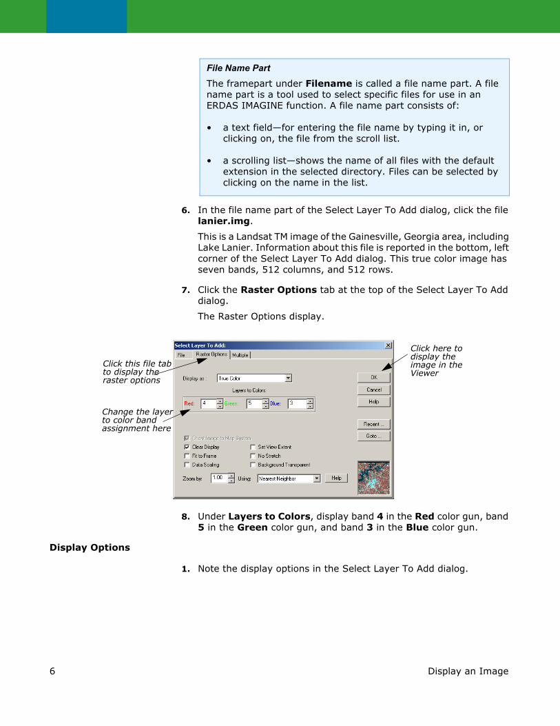
7. Click the Raster Options tab at the top of the Select Layer To Add dialog.
The Raster Options display.
8. Under Layers to Colors, display band 4 in the Red color gun, band 5 in the Green color gun, and band 3 in the Blue color gun.
Display Options
1. Note the display options in the Select Layer To Add dialog.
File Name PartThe framepart under Filename is called a file name part. A file name part is a tool used to select specific files for use in an ERDAS IMAGINE function. A file name part consists of:
• a text field—for entering the file name by typing it in, or clicking on, the file from the scroll list.
• a scrolling list—shows the name of all files with the default extension in the selected directory. Files can be selected by clicking on the name in the list.
Click this file tab to display the raster options
Click here to
image in the display the
Viewer
Change the layer to color band assignment here
7Display an Image
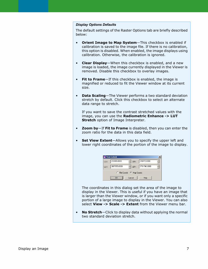
Display Options DefaultsThe default settings of the Raster Options tab are briefly described below:
• Orient Image to Map System—This checkbox is enabled if calibration is saved to the image file. If there is no calibration, this option is disabled. When enabled, the image displays using calibration. Otherwise, the calibration is ignored.
• Clear Display—When this checkbox is enabled, and a new image is loaded, the image currently displayed in the Viewer is removed. Disable this checkbox to overlay images.
• Fit to Frame—If this checkbox is enabled, the image is magnified or reduced to fit the Viewer window at its current size.
• Data Scaling—The Viewer performs a two standard deviation stretch by default. Click this checkbox to select an alternate data range to stretch.
If you want to save the contrast stretched values with the image, you can use the Radiometric Enhance -> LUT Stretch option of Image Interpreter.
• Zoom by—If Fit to Frame is disabled, then you can enter the zoom ratio for the data in this data field.
• Set View Extent—Allows you to specify the upper left and lower right coordinates of the portion of the image to display.
The coordinates in this dialog set the area of the image to display in the Viewer. This is useful if you have an image that is larger than the Viewer window, or if you want only a specific portion of a large image to display in the Viewer. You can also select View -> Scale -> Extent from the Viewer menu bar.
• No Stretch—Click to display data without applying the normal two standard deviation stretch.

8 Utility Menu Options
2. Click OK in the Select Layer To Add dialog to display the file.
The file lanier.img displays in the Viewer. The name of the file and the layers selected are written in the Viewer title bar.
Utility Menu Options
The Utility menu on the Viewer enables you to access four separate groups of functions:
• inquiry functions
• measurement tool
• layer viewing
Display Options Defaults, Continued
• Background Transparent—Click to make the background of grayscale, pseudocolor, and true color areas transparent—the layer underneath shows through. Background areas are automatically transparent in thematic layers.
• Using—Resampling is appropriate if the image is magnified (a magnification factor greater than one). Use one of the following resampling methods: Nearest Neighbor, Bilinear Interpolation, Cubic Convolution, and Bicubic Spline.
Click here to minimize the window
The title bar showsthe Viewer numberand name of imagedisplayed
Drag on anyof the cornersto resize the Viewer
In the title bar,
move the Viewerhold and drag to
Use the scroll barsto roam in an image
Single-line help and coordinates display in this Status Bar
9Utility Menu Options
• information
Each function group is separated by a line in the dropdown menu.
Use Inquiry Functions You can query a displayed image for information about each pixel using the inquiry functions.
The file lanier.img must be displayed in a Viewer.
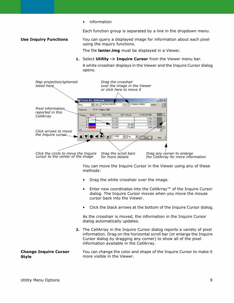
1. Select Utility -> Inquire Cursor from the Viewer menu bar.
A white crosshair displays in the Viewer and the Inquire Cursor dialog opens.
You can move the Inquire Cursor in the Viewer using any of these methods:
• Drag the white crosshair over the image.
• Enter new coordinates into the CellArray™ of the Inquire Cursor dialog. The Inquire Cursor moves when you move the mouse cursor back into the Viewer.
• Click the black arrows at the bottom of the Inquire Cursor dialog.
As the crosshair is moved, the information in the Inquire Cursor dialog automatically updates.
2. The CellArray in the Inquire Cursor dialog reports a variety of pixel information. Drag on the horizontal scroll bar (or enlarge the Inquire Cursor dialog by dragging any corner) to show all of the pixel information available in the CellArray.
Change Inquire Cursor Style
You can change the color and shape of the Inquire Cursor to make it more visible in the Viewer.
Drag the crosshair over the image in the Viewer or click here to move it
Drag the scroll bars
Map projection/spheroid listed here
Drag any corner to enlarge the CellArray for more information for more details
Pixel informationreported in thisCellArray
Click arrows to move
the Inquire cursor
Click the circle to move the Inquire cursor to the center of the image
10 Utility Menu Options
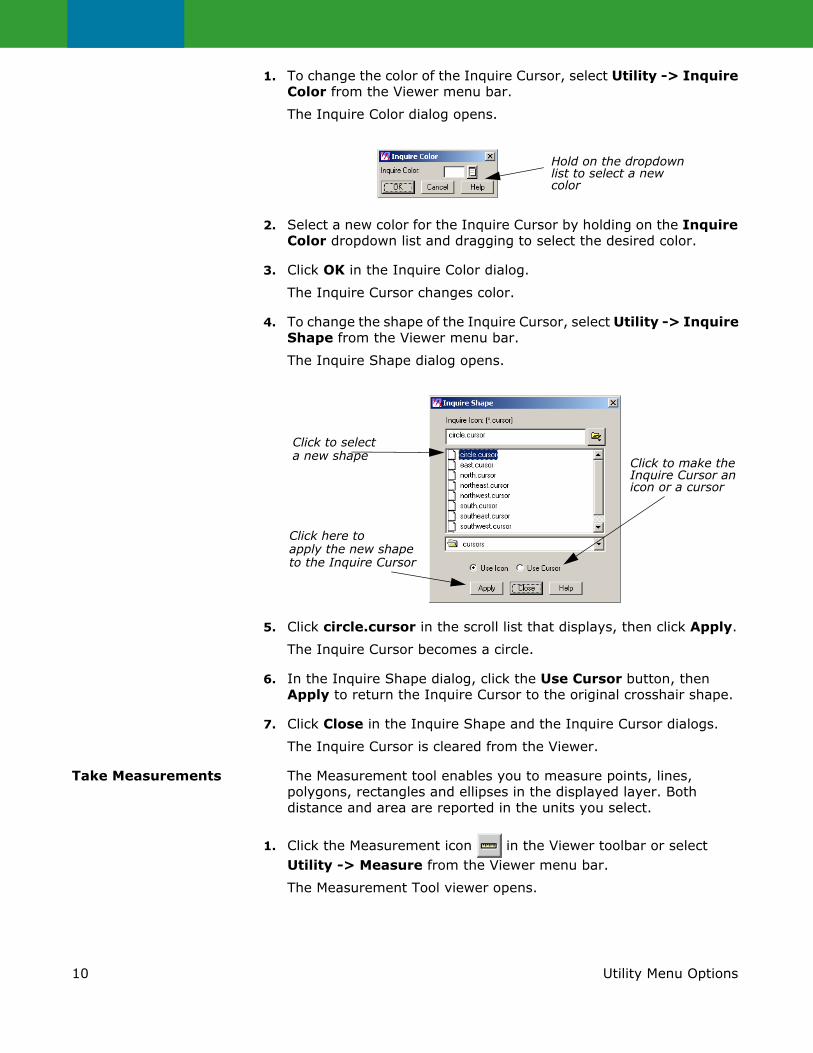
1. To change the color of the Inquire Cursor, select Utility -> Inquire Color from the Viewer menu bar.
The Inquire Color dialog opens.
2. Select a new color for the Inquire Cursor by holding on the Inquire Color dropdown list and dragging to select the desired color.
3. Click OK in the Inquire Color dialog.
The Inquire Cursor changes color.
4. To change the shape of the Inquire Cursor, select Utility -> Inquire Shape from the Viewer menu bar.
The Inquire Shape dialog opens.
5. Click circle.cursor in the scroll list that displays, then click Apply.
The Inquire Cursor becomes a circle.
6. In the Inquire Shape dialog, click the Use Cursor button, then Apply to return the Inquire Cursor to the original crosshair shape.
7. Click Close in the Inquire Shape and the Inquire Cursor dialogs.
The Inquire Cursor is cleared from the Viewer.
Take Measurements The Measurement tool enables you to measure points, lines, polygons, rectangles and ellipses in the displayed layer. Both distance and area are reported in the units you select.
1. Click the Measurement icon in the Viewer toolbar or select Utility -> Measure from the Viewer menu bar.
The Measurement Tool viewer opens.
Hold on the dropdown list to select a new color
Click to make the Inquire Cursor an icon or a cursor
Click here to apply the new shapeto the Inquire Cursor
Click to selecta new shape

11Utility Menu Options
2. Click the Measure Positions icon in the Measurement toolbar. This tool gives the individual point coordinates (x, y) in the image.
3. Move the cursor into the Viewer and click anywhere.
In the Measurement Tool viewer, the location of the point displays in the type of units in which the file is saved. You may select different display units from the dropdown lists in the top toolbar.
4. Next, click the Polyline icon in the Measurement Tool viewer toolbar.
5. Move the cursor into the Viewer and click once at the beginning of a line feature then drag the mouse to extend the line along the feature. Click to add a vertex at each point. Middle-click (or double-click, depending on how your Preferences are set) to end the measurement.
The length displays in the Measurement Tool CellArray.
6. Click the Print icon to print and a Print dialog opens, which allows you to enter or select the printer to be used.
Click to print
Click to locate point coordinates
The Measurement Tool
The Measurement Tool can create a new annotation layer on top of your image. Simply click the Annotation tool and a new layer is automatically created. While this tool is enabled, the measurement features (points, polylines, polygons, rectangles, ellipses, etc.) are added to the annotation layer as well as a text box containing the measured values. Click the tool again to turn this feature off.
The annotation layer may be saved and used with other images with the same geographic area.
NOTE: These annotation objects may be moved and resized, but the measured values in the text boxes are not updated.
12 View Menu Options
7. Select the Printer and click Print (or OK) in the Print dialog. If you do not wish to print, click Cancel.
8. Experiment with the other measurement tools if you like, and when you are done, click the Close button in the top toolbar.
You are asked if you want to save the measurements. Save them if
you like. You can click the Save icon at any time to save your measurements.
Click the Help button to view the On-Line Help for the measurement tools.
View Menu Options
Arrange Layers ERDAS IMAGINE should be running, and lanier.img should be displayed in a Viewer.
1. In the Viewer toolbar, click the Open icon to open another layer on top of lanier.img.
The Select Layer To Add dialog opens.
2. In the Select Layer To Add dialog under File name, click lnsoils.img. This is a thematic soils file of the Gainesville, Georgia area.
3. Click the Raster Options tab at the top of the Select Layer To Add dialog.
4. Check to be sure that the Clear Display checkbox is disabled (not selected), so that lanier.img is not cleared from the Viewer when lnsoils.img displays.
5. Click OK in the Select Layer To Add dialog to display the file.
Now, both lanier.img and lnsoils.img are displayed in the same Viewer, with lnsoils.img on top.
6. To bring lanier.img to the top of the Viewer, select View -> Arrange Layers from the Viewer menu bar.
The Arrange Layers dialog opens.

13View Menu Options
7. In the Arrange Layers dialog, drag the lanier.img box above the lnsoils.img box, as illustrated above.
When you release the mouse button, the layers are rearranged in the Arrange Layers dialog so that the lanier.img box is first.
8. Click Apply in the Arrange Layers dialog to redisplay the layers in their new order in the Viewer.
The layers are now reversed.
9. Click Close in the Arrange Layers dialog.
Zoom In this section, you zoom in by a factor of 2 and create a magnifier window. Once the image enlarges, you can roam through it.
lanier.img should be displayed on top of lnsoils.img in a Viewer at a magnification of 1 (this is the case if you have been following through this tour guide from the beginning).
1. Select View -> Zoom -> In by 2 from the Viewer menu bar.
The images are redisplayed at a magnification factor of 2.
The Zoom options are also available from:
— the Quick View menu (right-hold on the Viewer image) under Zoom -> Zoom In by 2
— the Viewer toolbar by clicking this icon .
2. Move the scroll bars on the bottom and side of the Viewer window to view other parts of the image.
To move by small increments, you can click the small triangles at either end of the scroll bars. To move by larger increments, drag the scroll bars.
Click and drag this box to the topto change theorder of the displayed layers
Click here toredisplay layersin the new order
14 View Menu Options
You can also enlarge the Viewer window by dragging any corner.
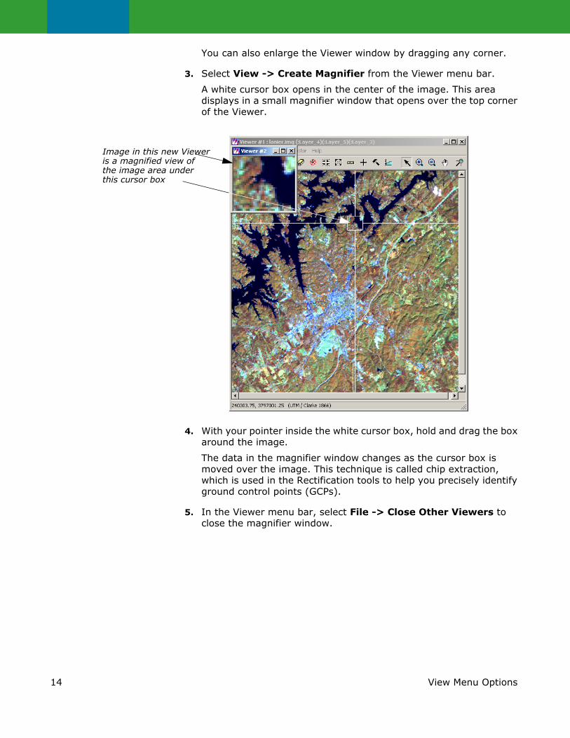
3. Select View -> Create Magnifier from the Viewer menu bar.
A white cursor box opens in the center of the image. This area displays in a small magnifier window that opens over the top corner of the Viewer.
4. With your pointer inside the white cursor box, hold and drag the box around the image.
The data in the magnifier window changes as the cursor box is moved over the image. This technique is called chip extraction, which is used in the Rectification tools to help you precisely identify ground control points (GCPs).
5. In the Viewer menu bar, select File -> Close Other Viewers to close the magnifier window.
Image in this new Vieweris a magnified view ofthe image area underthis cursor box
15View Menu Options
Other methods of zooming in and out of imagery are Animated Zoom, Box Zoom, and Real-time Zoom.
Animated Zoom Animated Zoom enables you to zoom in and out of the Viewer’s image in a series of steps that are similar to animation. The image is resampled after it is magnified or reduced.
Display lanier.img in the Viewer.
1. Select Session -> Preferences.
2. In the Preference Editor dialog, select Viewer from the Category list.
3. Click the checkbox for Enable Animated Zoom.
4. Click User Save then Close in dialog, and go back to the Viewer.
5. Click the Zoom In By Two icon .
The Viewer zooms into the image in a simulated animation by a factor of 2. The Viewer center is maintained.
6. Click the Zoom Out By Two icon .
The Viewer zooms out of the image in a simulated animation by a factor of 2. The Viewer center is maintained.
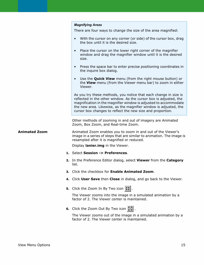
Magnifying AreasThere are four ways to change the size of the area magnified:
• With the cursor on any corner (or side) of the cursor box, drag the box until it is the desired size.
• Place the cursor on the lower right corner of the magnifier window and drag the magnifier window until it is the desired size.
• Press the space bar to enter precise positioning coordinates in the inquire box dialog.
• Use the Quick View menu (from the right mouse button) or the View menu (from the Viewer menu bar) to zoom in either Viewer.
As you try these methods, you notice that each change in size is reflected in the other window. As the cursor box is adjusted, the magnification in the magnifier window is adjusted to accommodate the new area. Likewise, as the magnifier window is adjusted, the cursor box changes to reflect the new size and proportion.
16 View Menu Options
7. Click either the Interactive Zoom In or the Interactive Zoom Out
icon .
8. Click a location on the image.
The Viewer recenters the image to that location and zooms in or out in a simulated animation by a factor of 2.
Animated zoom also works with View -> Zoom -> In by X and Out by X.
Box Zoom Box Zoom is used to select a boxed area in the image. When zooming in or out by using the zoom recentering icons, the boxed image enlarges or reduces within the Viewer.
Display lanier.img in the Viewer.
1. Select Session ->Preferences.
2. In the Preference Editor dialog, select Viewer from the Category list.
3. Click to select Enable Box Zoom.
4. Click User Save then Close in dialog, and go back to the Viewer.
5. Click the Interactive Zoom In icon.
6. Click and drag a box in the image.
The selected area of the image is magnified to fit the Viewer.
7. Select the Interactive Zoom Out icon.
8. Click and drag a box in the image.
The area displayed in the Viewer is reduced to fit in the box. Space surrounding the reduced image is populated with available imagery.
Real-time Zoom When you select either of the Interactive Zoom tools, you can to zoom into and out of images in real time by holding the middle mouse button and moving the mouse upward and downward over the image.
NOTE: You can also hold down the Control key and press on the left mouse button to zoom in real time.
Display lanier.img in the Viewer. There is no need to set up a preference for this feature.
1. Select either of the Interactive Zoom icons.
2. Position the cursor in the Viewer, and hold the middle mouse button.
3. Move the mouse forward to zoom in on the image.
17View Menu Options
The image magnifies at a constant rate, depending on how far forward you move the mouse.
4. Hold the middle mouse button and move the mouse backward.
The image reduces at a constant rate, depending on how far downward on the image you move the mouse.
Display Two Images Two or more Viewers can be geographically or spectrally linked so that when you roam in one image, that area is simultaneously displayed in the linked Viewer(s).
The file lanier.img should be displayed on top of lnsoils.img in a Viewer window, at a magnification of 2.
1. Drag on a lower corner of the Viewer so that it occupies the entire left half of the screen.
2. In the Viewer menu bar, select View -> Split -> Split Horizontal.
The Viewer is divided in half, horizontally, to form two Viewers.
3. In the toolbar of the new Viewer, click the Open icon .
The Select Layer To Add dialog opens.
4. In the Select Layer To Add dialog under File name, click the file lnsoils.img.
5. Click the Raster Options tab at the top of the dialog.
6. Confirm that Zoom by is set to 1.00.
7. Click OK in the Select Layer To Add dialog.
The file lnsoils.img displays in the second Viewer.
Link Viewers
1. In the first Viewer, select View -> Link/Unlink Viewers -> Geographical.
The Link/Unlink Instructions display.
2. Move your pointer to the second Viewer.
The pointer becomes a Link symbol .
Types of Linking
• Geographically linked—the same image area displays in all linked Viewers.
• Spectrally linked—enhancements made to an image are also made in other Viewers if that same image, or portions of it, are displayed in other Viewers.
18 View Menu Options
3. Move the pointer to the first Viewer.
The No Link symbol displays as the cursor in the first Viewer. Clicking in this Viewer discontinues the link operation.
4. To link the Viewers, click anywhere in the second Viewer.
The two Viewers are now linked. A white cursor box opens over the image in the second Viewer, indicating the image area displayed in the first Viewer.
You can move and resize this cursor box as desired, and the image area in the first Viewer reflects each change. This is similar to the magnification box you used earlier.
Compare Images
1. Drag the cursor box in the second Viewer to a new location. The image area selected in the second Viewer displays in the first Viewer.
2. Drag the scroll bars in the first Viewer to roam in the image.
The white cursor box in the second Viewer moves as the image area in the first Viewer changes.
You could also use the Roam icon in the Viewer toolbar to roam over the image. Just move the hand across the Viewer image to change the view.
Unlink Viewers
1. In either Viewer, select View -> Link/Unlink Viewers -> Geographical to unlink the Viewers.
The Link/Unlink Instructions display.
2. Move the pointer to the other Viewer.
The unlink cursor displays.
3. Click anywhere inside the Viewer to unlink the Viewers.
4. In the menu bar of the second Viewer, select File -> Close.
The second Viewer closes.
5. In the first Viewer, select File -> Clear to clear the Viewer.
19Raster Menu Options
Raster Menu Options
Create an AOI Layer These options allow you to define an AOI in the image, excluding other parts of the image. Specific processes can be applied to this AOI only, which can save considerable time and disk space. The option to use a specified AOI for processing is available from many dialogs throughout ERDAS IMAGINE.
This exercise tells you how to create an AOI layer that can be saved as a file and recalled for later use.
NOTE: Each Viewer can display only one AOI layer at a time.
Display lanier.img in a Viewer. You must have an image displayed in the Viewer to create an AOI layer.
1. Select File -> New -> AOI Layer from the Viewer menu bar.
ERDAS IMAGINE creates an AOI layer.
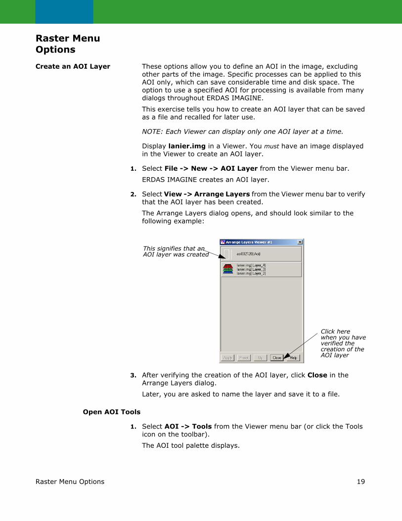
2. Select View -> Arrange Layers from the Viewer menu bar to verify that the AOI layer has been created.
The Arrange Layers dialog opens, and should look similar to the following example:
3. After verifying the creation of the AOI layer, click Close in the Arrange Layers dialog.
Later, you are asked to name the layer and save it to a file.
Open AOI Tools
1. Select AOI -> Tools from the Viewer menu bar (or click the Tools icon on the toolbar).
The AOI tool palette displays.
This signifies that an AOI layer was created
Click herewhen you haveverified thecreation of theAOI layer
20 Raster Menu Options
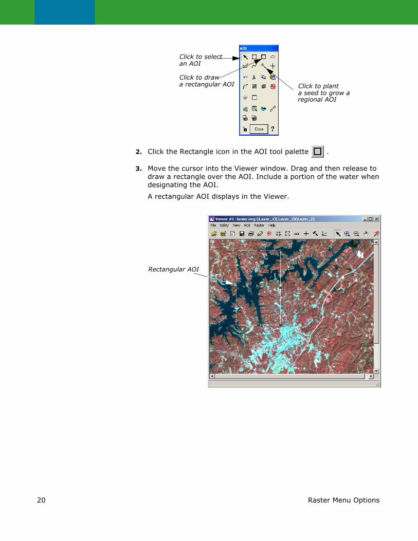
2. Click the Rectangle icon in the AOI tool palette .
3. Move the cursor into the Viewer window. Drag and then release to draw a rectangle over the AOI. Include a portion of the water when designating the AOI.
A rectangular AOI displays in the Viewer.
Click to drawa rectangular AOI Click to plant
a seed to grow aregional AOI
Click to selectan AOI
Rectangular AOI
21Raster Menu Options
Select Styles
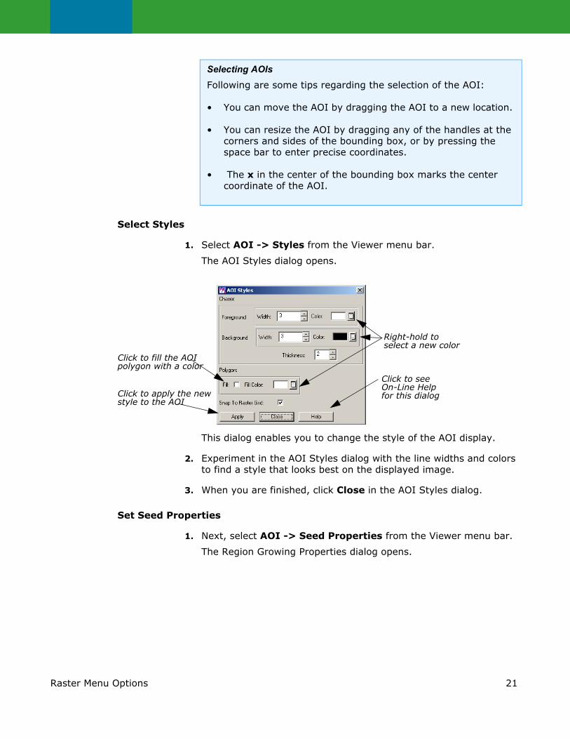
1. Select AOI -> Styles from the Viewer menu bar.
The AOI Styles dialog opens.
This dialog enables you to change the style of the AOI display.
2. Experiment in the AOI Styles dialog with the line widths and colors to find a style that looks best on the displayed image.
3. When you are finished, click Close in the AOI Styles dialog.
Set Seed Properties
1. Next, select AOI -> Seed Properties from the Viewer menu bar.
The Region Growing Properties dialog opens.
Selecting AOIsFollowing are some tips regarding the selection of the AOI:
• You can move the AOI by dragging the AOI to a new location.
• You can resize the AOI by dragging any of the handles at the corners and sides of the bounding box, or by pressing the space bar to enter precise coordinates.
• The x in the center of the bounding box marks the center coordinate of the AOI.
Click to apply the new style to the AOI
Click to see On-Line Help for this dialog
Click to fill the AOI polygon with a color
Right-hold to select a new color
22 Raster Menu Options
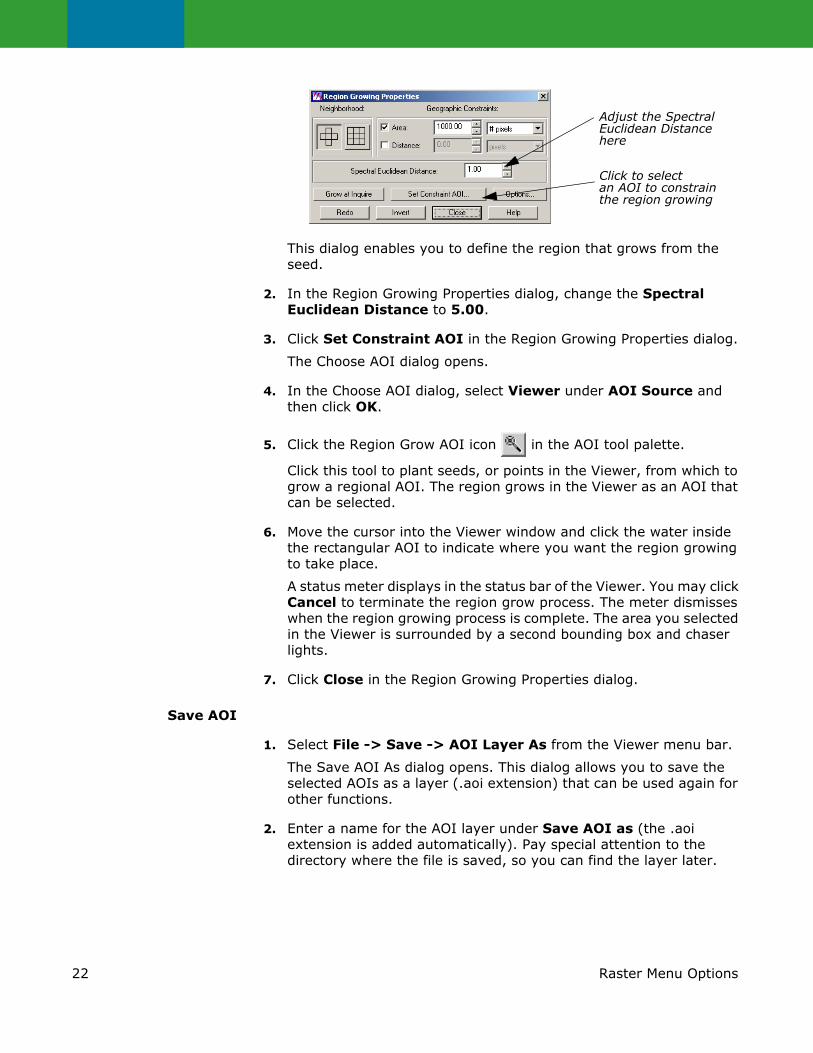
This dialog enables you to define the region that grows from the seed.
2. In the Region Growing Properties dialog, change the Spectral Euclidean Distance to 5.00.
3. Click Set Constraint AOI in the Region Growing Properties dialog.
The Choose AOI dialog opens.
4. In the Choose AOI dialog, select Viewer under AOI Source and then click OK.
5. Click the Region Grow AOI icon in the AOI tool palette.
Click this tool to plant seeds, or points in the Viewer, from which to grow a regional AOI. The region grows in the Viewer as an AOI that can be selected.
6. Move the cursor into the Viewer window and click the water inside the rectangular AOI to indicate where you want the region growing to take place.
A status meter displays in the status bar of the Viewer. You may click Cancel to terminate the region grow process. The meter dismisses when the region growing process is complete. The area you selected in the Viewer is surrounded by a second bounding box and chaser lights.
7. Click Close in the Region Growing Properties dialog.
Save AOI
1. Select File -> Save -> AOI Layer As from the Viewer menu bar.
The Save AOI As dialog opens. This dialog allows you to save the selected AOIs as a layer (.aoi extension) that can be used again for other functions.
2. Enter a name for the AOI layer under Save AOI as (the .aoi extension is added automatically). Pay special attention to the directory where the file is saved, so you can find the layer later.
Click to select an AOI to constrain the region growing
Adjust the Spectral Euclidean Distance here

23Raster Menu Options
If you wanted to save specific AOIs only, you could turn on the Selected Only checkbox in the Save AOI As dialog, and only selected AOIs would be saved to a file.
3. Click OK in the Save AOI As dialog.
This layer can now be used in any dialog where a function can be applied to a specific AOI layer. You can also edit this layer at any time, adding or deleting areas.
Arrange Layers
1. Select View -> Arrange Layers from the Viewer menu bar.
The Arrange Layers dialog opens.
2. In the Arrange Layers dialog, right-hold over the AOI Layer and select Delete Layer from the AOI Options menu.
3. Click Apply and then Close in the Arrange Layers dialog.
The file lanier.img is redisplayed in the Viewer without the AOI layer.
Adjust Image Contrast When images are displayed in ERDAS IMAGINE, a linear contrast stretch is applied to the data file values, but you can further enhance the image using a variety of techniques.
The file lanier.img should be displayed in a Viewer.
1. In the Viewer menu bar, select Raster -> Contrast -> Brightness/Contrast.
The Contrast Tool dialog opens.
2. In the Contrast Tool dialog, change the numbers and/or use the slider bars to adjust the image brightness and contrast.
3. Click Apply.
The image in the Viewer is redisplayed with new brightness values.
4. Click Reset and Apply in the Contrast Tool dialog to undo any changes made to the Viewer image.
Adjust brightness here
Adjust contrast here
Click here to reset to original contrast
Click here or here to apply changes

24 Raster Menu Options
5. Click Close in the Contrast Tool dialog.
Use Piecewise Linear Stretches
1. In the Viewer menu bar, select Raster -> Contrast -> Piecewise Contrast.
The Contrast Tool dialog for piecewise contrast opens.
2. With your pointer over the image in the Viewer, right-hold Quick View -> Inquire Cursor.
The Inquire Cursor dialog opens and an Inquire Cursor is placed in the Viewer.
Adjust contrast and brightness here
Specify range of lookup table to modify here
Set lookup table ranges here
Select color gun to affect
Click here to reset to the original lookup table
contrast
The Contrast ToolThis tool enables you to enhance a particular portion of an image by dividing the lookup table into three sections: low, middle, and high. You can enhance the contrast or brightness of any section using a single color gun at a time. This technique is very useful for enhancing image areas in shadow, or other areas of low contrast.
The brightness value for each range represents the midpoint of the total range of brightness values occupied by that range.
The contrast value for each range represents the percent of the available output range that particular range occupies.
As one slider bar is moved, the other is automatically adjusted, so that there is no gap in the lookup table. This tool is set up so that there are always pixels in each data file value from 0 to 255. You can manipulate the percentage of pixels in a particular range, but you cannot eliminate a range of data file values.

25Raster Menu Options
3. In the Viewer, drag the intersection of the Inquire Cursor to the lake. Move the Inquire Cursor over the water while keeping an eye on the lookup table values in the blue color gun, as reported in the Inquire Cursor dialog.
This gives you an idea of the range of data file values in the water. You can stretch this range to bring out more detail in the water.
4. In the Contrast Tool dialog, click Blue under Select Color.
5. Under Range Specifications, set the Low range From 34 To 55 and press Enter on your keyboard.
6. Drag the Brightness slider bar (the top slider bar) to 50.
7. Click Apply in the Contrast Tool dialog.
The water now has more contrast and shows more detail.
If your image is at a magnification of 1, this new detail may be difficult to see. You can zoom in to a magnification of 2 using the Quick View menu in the Viewer.
8. In the Contrast Tool dialog, click Reset and then Apply to return the image to the original lookup table values.
9. Click Close in the Contrast Tool dialog.
10. Click Close in the Inquire Cursor dialog.
Manipulate Histogram
1. In the Viewer menu bar, select Raster -> Contrast -> Breakpoints.
The Breakpoint Editor opens.
26 Raster Menu Options
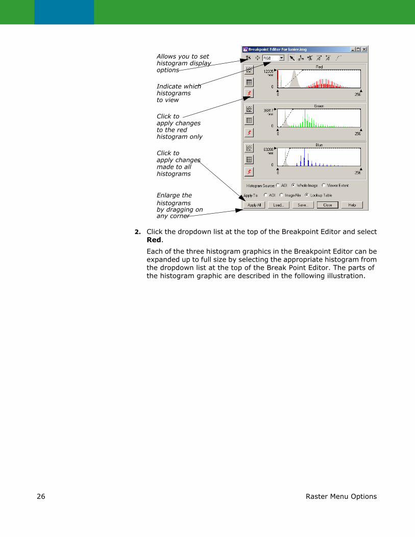
2. Click the dropdown list at the top of the Breakpoint Editor and select Red.
Each of the three histogram graphics in the Breakpoint Editor can be expanded up to full size by selecting the appropriate histogram from the dropdown list at the top of the Break Point Editor. The parts of the histogram graphic are described in the following illustration.
Indicate which histograms to view
Click to apply changes made to all histograms
Allows you to set histogram display options
Click to apply changes to the red histogram only
Enlarge the
by dragging on any corner
histograms

27Raster Menu Options
3. Click the dropdown list at the top of the Breakpoint Editor and select RGB.
All three histograms redisplay in the Breakpoint Editor.
4. Experiment by dragging the breakpoints of the lookup table graphs in the different color guns (Red, Green, and Blue).
5. Click Apply All in the Breakpoint Editor to view the results of your changes in the image.
6. To undo the edits you just made, select Raster -> Undo from the Viewer menu bar.
Adjust Shift/Bias
1. In the Breakpoint Editor, click the Shift/Bias icon on the toolbar.
The Shift/Bias Adjustment dialog opens.
The Y axis represents both the frequencies of the histogram and the range of output values for the lookup table
The X axis The histogram of the input values (white) does not change
The histogram of
represented frequency The highest
The lookup table
you manipulate the (red) changes as the output values
lookup table graph
range of values
range is 0 to 255)
represents the
(for 8-bit data, the
breakpoints graph with
(small squares)
Histogram Edit Tools

28 Raster Menu Options
The lookup table graph and the output histogram are updated in the Histogram Tool dialog as you manipulate the information in the Shift/Bias Adjustment dialog.
2. In the Shift/Bias Adjustment dialog, drag the Shift slider bar to the right.
Notice that the value in the number field to the left increases as you move the slider bar. This is the number of pixels that the lookup table graph is moved.
3. In the Shift/Bias Adjustment dialog, double-click the number in the Shift number field and change the number field to 20. Press Enter on your keyboard.
4. In the Breakpoint Editor, click Apply All.
The image is redisplayed using the new lookup table. It is very dark.
5. In the Shift/Bias Adjustment dialog, return the Shift value to 0.
6. In the Breakpoint Editor, click Apply All to return the image to its original contrast.
7. Repeat step 2 through step 6 using the Bias option.
8. When you are finished, click Close in the Shift/Bias Adjustment dialog.
Use Mouse Linear Mapping
1. In the Breakpoint Editor, click the Red Mouse Linear Mapping icon
, which is located on the left border of the Red histogram.
The Red Mouse Linear Mapping dialog opens.
Shift moves the lookup table graphleft and right (X direction)
Bias moves thelookup table graphup and down(Y direction)
29Raster Menu Options
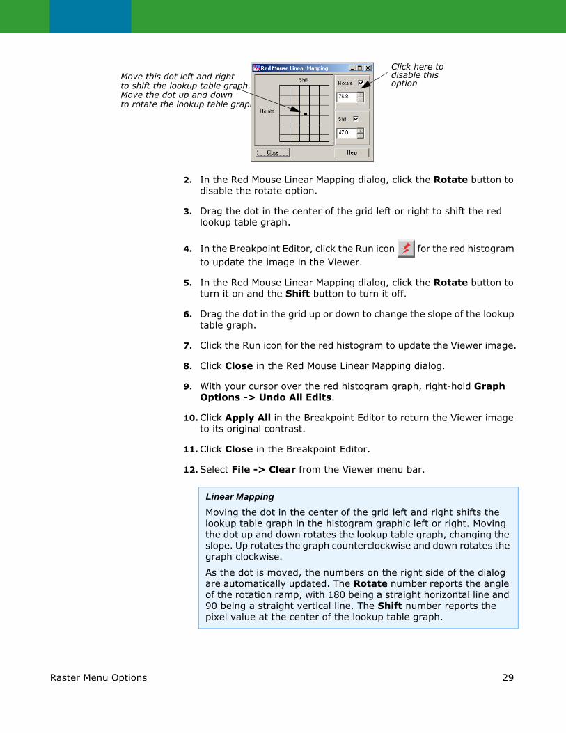
2. In the Red Mouse Linear Mapping dialog, click the Rotate button to disable the rotate option.
3. Drag the dot in the center of the grid left or right to shift the red lookup table graph.
4. In the Breakpoint Editor, click the Run icon for the red histogram to update the image in the Viewer.
5. In the Red Mouse Linear Mapping dialog, click the Rotate button to turn it on and the Shift button to turn it off.
6. Drag the dot in the grid up or down to change the slope of the lookup table graph.
7. Click the Run icon for the red histogram to update the Viewer image.
8. Click Close in the Red Mouse Linear Mapping dialog.
9. With your cursor over the red histogram graph, right-hold Graph Options -> Undo All Edits.
10. Click Apply All in the Breakpoint Editor to return the Viewer image to its original contrast.
11. Click Close in the Breakpoint Editor.
12. Select File -> Clear from the Viewer menu bar.
Move this dot left and right to shift the lookup table graph. Move the dot up and down to rotate the lookup table graph.
Click here to disable this option
Linear MappingMoving the dot in the center of the grid left and right shifts the lookup table graph in the histogram graphic left or right. Moving the dot up and down rotates the lookup table graph, changing the slope. Up rotates the graph counterclockwise and down rotates the graph clockwise.
As the dot is moved, the numbers on the right side of the dialog are automatically updated. The Rotate number reports the angle of the rotation ramp, with 180 being a straight horizontal line and 90 being a straight vertical line. The Shift number reports the pixel value at the center of the lookup table graph.
30 Raster Editor
Raster Editor The Raster Editor enables you to edit portions of the displayed image using various tools in the Viewer Raster menu. When a specific raster editing tool is in use, that tool locks the Viewer, therefore, work with one tool must be completed before opening another one.
All of the dialogs that accompany the raster editing tools contain a preview window, which enables you to view the changes you make to the Viewer image before you click Apply.
Prepare (UNIX)
You must have a writable file displayed to use this function. Follow the steps below to create a writable file to work with.
1. In a command window, copy lndem.img to testdem.img by typing the following (without a carriage return):
cp <ERDAS_Data_Home>/examples/lndem.img <your directory path>/testdem.img
Press Enter on your keyboard.
2. Change read/write permissions by typing the following in the command window:
chmod 644 testdem.img
Press Enter on your keyboard and close the command window.
Prepare (PC)
1. Open the Explorer.
2. Copy lndem.img from the <ERDAS_Data_Home>/examples directory to the directory of your choice.
3. Right-click and select Rename to rename the file testdem.img.
4. Right-click the file, and select Properties.
5. In the Attributes section of the General tab, make sure Read-only is not checked.
6. Click OK in the Properties dialog.
Open the Image
1. Open testdem.img in the Viewer.
This is a DEM file of the Gainesville, Georgia area, corresponding to the lanier.img data you have been using.
2. If it is not already displayed, select AOI -> Tools from the Viewer menu bar to open the AOI tool palette.
The AOI tool palette displays. The AOI tools are used to define the area(s) to be edited.
31Raster Editor
3. Click the Ellipse icon in the AOI tool palette and then drag near the center of the Viewer image to draw an elliptical AOI, measuring about 1” to 2” in diameter.
When the mouse button is released, the AOI is surrounded by chaser lights and a bounding box.
Interpolate
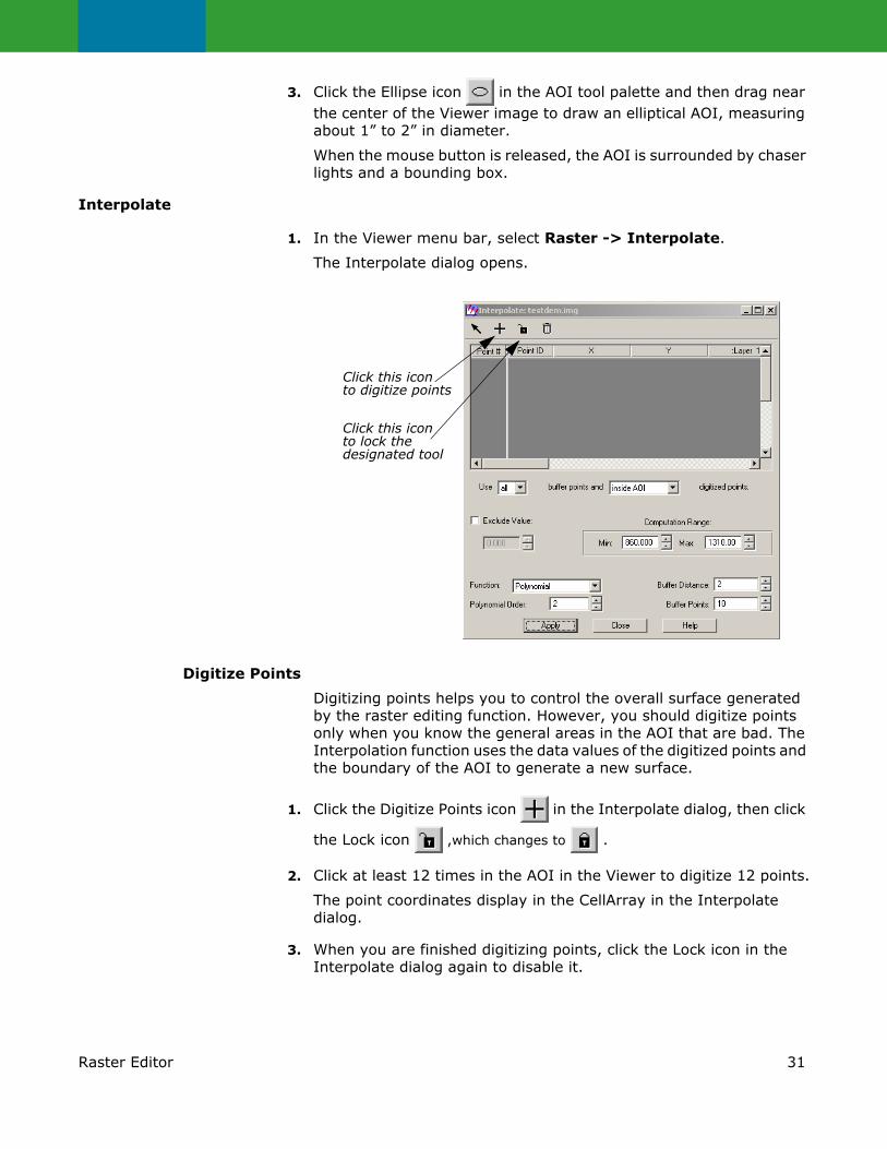
1. In the Viewer menu bar, select Raster -> Interpolate.
The Interpolate dialog opens.
Digitize Points
Digitizing points helps you to control the overall surface generated by the raster editing function. However, you should digitize points only when you know the general areas in the AOI that are bad. The Interpolation function uses the data values of the digitized points and the boundary of the AOI to generate a new surface.
1. Click the Digitize Points icon in the Interpolate dialog, then click
the Lock icon ,which changes to .
2. Click at least 12 times in the AOI in the Viewer to digitize 12 points.
The point coordinates display in the CellArray in the Interpolate dialog.
3. When you are finished digitizing points, click the Lock icon in the Interpolate dialog again to disable it.
Click this icon to lock the designated tool
Click this icon to digitize points

32 Raster Editor
4. In the Interpolate dialog under Buffer Points, enter 25 to allow up to 25 points in the computation.
5. In the Interpolate dialog under Polynomial Order, enter 3 to increase the polynomial order of interpolation.
6. Click Apply in the Interpolate dialog.
7. An Attention box displays, asking if you want to remove the data stretch lookup table. Click Yes.
8. A Warning box displays, suggesting that you recalculate the statistics. Click OK.
The new surface displays inside the AOI.
9. Observe the changes in the AOI and then select Raster -> Undo from the Viewer menu bar.
The data values return to the original values. This lets you undo the edit without changing the original data values.
NOTE: Undo works only for the last edit applied.
10. Click Close in the Interpolate dialog.
Fill with Constant Value If the area to be edited is a flat surface, you may use a constant value to replace the bad data values.
1. Select Raster -> Fill from the Viewer menu bar.
The Area Fill dialog opens.
2. In the Area Fill dialog, click Apply to accept the Constant function and its defaults.
The AOI is replaced with a Constant value of zero—the area is black.
3. Select Raster -> Undo from the Viewer menu bar.
The image returns to the original values.
4. In the Area Fill dialog, enter 1500 in the Fill With number field and click Apply.
The preview window displays what the AOI fill looks like
Click here to apply the specified area fill
33Raster Attribute Editor
Now the AOI fill area is white.
5. Select Raster -> Undo from the Viewer menu bar.
The image returns to the original values.
Set Global Value
1. In the Area Fill dialog, click the Function dropdown list and select Majority.
This option uses the majority of the pixel values in the AOI to replace all values in the AOI.
2. Click Apply in the Area Fill dialog.
The AOI displays the newly generated surface.
3. After observing the changes, select Raster -> Undo from the Viewer menu bar.
4. Click Close in the Area Fill dialog.
5. Select File -> Clear from the Viewer menu bar.
Save the AOI layer in the Viewer if you like.
Raster Attribute Editor
You can easily change the class colors in a thematic file. Here, you change the colors in lnsoils.img.
Change Color Attribute Display lnsoils.img in a Viewer.
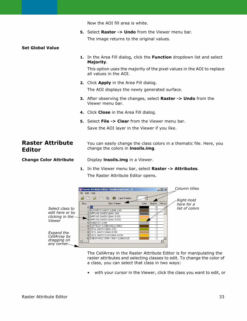
1. In the Viewer menu bar, select Raster -> Attributes.
The Raster Attribute Editor opens.
The CellArray in the Raster Attribute Editor is for manipulating the raster attributes and selecting classes to edit. To change the color of a class, you can select that class in two ways:
• with your cursor in the Viewer, click the class you want to edit, or
Expand the
Column titles
Right-holdhere for alist of colors
CellArray by dragging on any corner
Select class toedit here or byclicking in theViewer
34 Raster Attribute Editor
• with your cursor in the Row column of the Raster Attribute Editor CellArray, click the class to edit.
You use both methods in the following examples.
2. Move your cursor inside the Viewer and click an area.
That class is highlighted in yellow in the Raster Attribute Editor CellArray, and the current color assigned to that class is shown in the bar underneath the Color column.
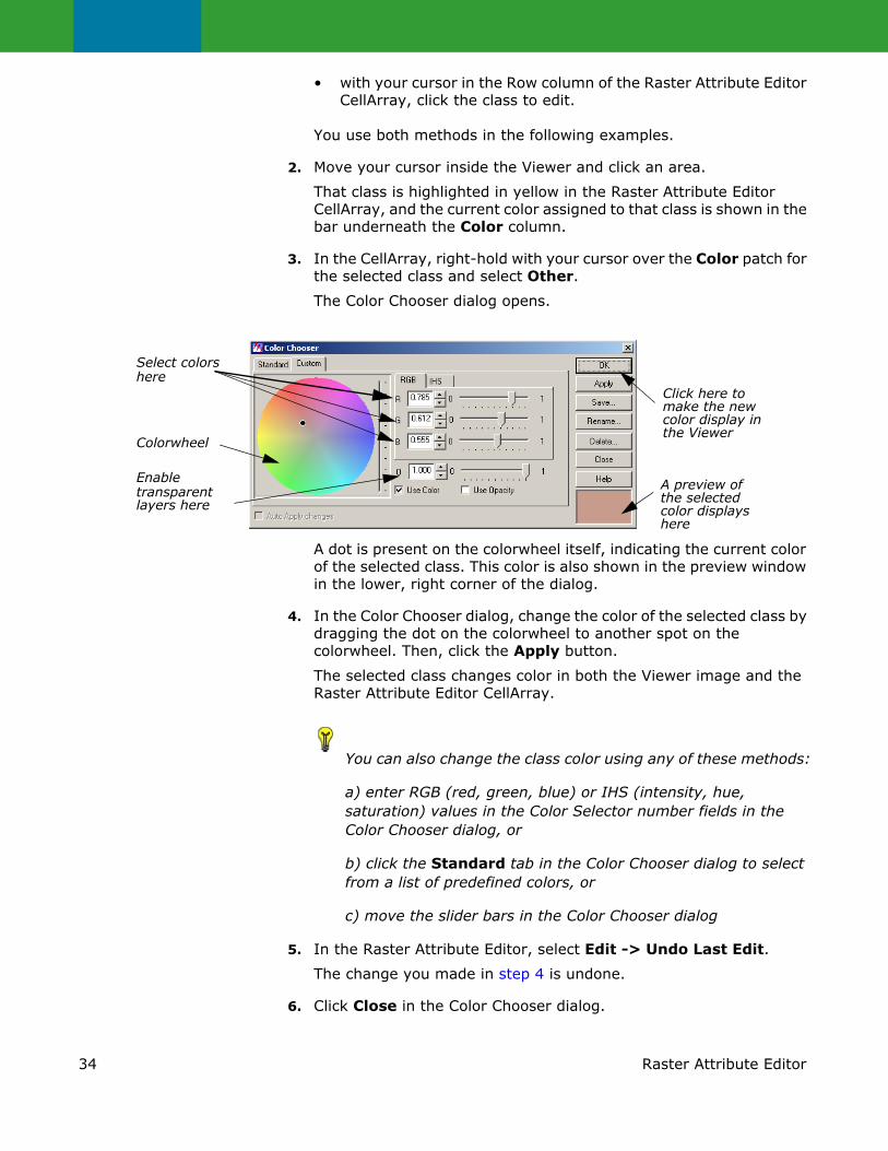
3. In the CellArray, right-hold with your cursor over the Color patch for the selected class and select Other.
The Color Chooser dialog opens.
A dot is present on the colorwheel itself, indicating the current color of the selected class. This color is also shown in the preview window in the lower, right corner of the dialog.
4. In the Color Chooser dialog, change the color of the selected class by dragging the dot on the colorwheel to another spot on the colorwheel. Then, click the Apply button.
The selected class changes color in both the Viewer image and the Raster Attribute Editor CellArray.
You can also change the class color using any of these methods:
a) enter RGB (red, green, blue) or IHS (intensity, hue, saturation) values in the Color Selector number fields in the Color Chooser dialog, or
b) click the Standard tab in the Color Chooser dialog to select from a list of predefined colors, or
c) move the slider bars in the Color Chooser dialog
5. In the Raster Attribute Editor, select Edit -> Undo Last Edit.
The change you made in step 4 is undone.
6. Click Close in the Color Chooser dialog.
Select colors here
Enable transparent A preview of
color display in
color displays
Click here to make the new
the Viewer
the selected
here
Colorwheel
layers here
35Raster Attribute Editor
7. Select File -> Close from the Raster Attribute Editor.
Make Layers Transparent If you have more than one file displayed in a Viewer, you can make specific classes or entire files transparent. In this example, you make the overlaid soils partially transparent so that the Landsat TM information shows through.
1. Display lanier.img over lnsoils.img in a Viewer. Be sure that the Clear Display checkbox is disabled under Raster Options when you are in the Select Layer To Add dialog.
2. In the Viewer menu bar, select View -> Arrange Layers.
The Arrange Layers dialog opens.
3. In the Arrange Layers dialog, drag the lnsoils.img box on top of the lanier.img box.
4. Click Apply, then Close in the Arrange Layers dialog.
Edit Raster Attributes
1. Select Raster -> Attributes from the Viewer menu bar.
The Raster Attribute Editor displays.
The objective is to select a class that covers a section of lanier.img that you would like to see through lnsoil.img. Then, you can make that class transparent.
2. Select the class to become transparent, either by clicking in the Viewer or in the Row column of the CellArray.
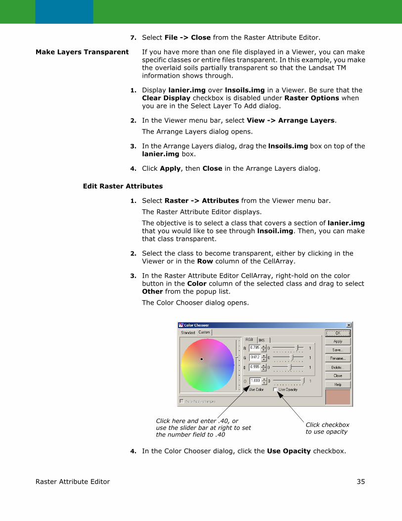
3. In the Raster Attribute Editor CellArray, right-hold on the color button in the Color column of the selected class and drag to select Other from the popup list.
The Color Chooser dialog opens.
4. In the Color Chooser dialog, click the Use Opacity checkbox.
Click here and enter .40, or use the slider bar at right to set the number field to .40
Click checkbox to use opacity

36 Raster Attribute Editor
5. At O (which stands for Opacity), change the number to .40 (opacity percentage of 40) using either the number field or the slider bar.
6. Click Apply in the Color Chooser dialog.
The selected color becomes partially transparent, allowing you to see lanier.img underneath.
7. Experiment with different ways to change class color and opacity.
8. When you are finished, click Close in the Color Chooser dialog.
Manipulate CellArray Information
1. With your cursor in the title bar of the Raster Attribute Editor, drag it to the top of your screen.
2. Drag one of the bottom corners of the Raster Attribute Editor down until all rows of theCellArray are visible.
3. Drag the corners of the Raster Attribute Editor horizontally until all columns are visible.
NOTE: The CellArray probably occupies most of your screen.
Select RowsTo select one row, simply click in the Row column of the desired row. That row is highlighted in yellow. You can select sequential rows by middle-clicking in additional rows. Shift-click in a selected row to deselect a row. You can also select rows using the Row Selection menu that opens when you right-hold in the Row column.
Select ColumnsTo select one column, click in the title box of the desired column. That column is highlighted in blue. You can select multiple columns by middle-clicking in the title bar of additional columns. Shift-click in a selected column to deselect it.
Choose Column OptionsMany column options are available from the Column Options menu, which opens when you right-hold in a column title bar. You can have multiple columns and rows selected at the same time.
You use many of these features in the following steps.
Resize ColumnsYou can make each column in the CellArray narrower and then reduce the width of the entire dialog, so that it takes up less room.

37Raster Attribute Editor
Edit Column Properties
1. Click the Column icon in the Raster Attribute Editor.
The Column Properties dialog opens.
2. In the Column Properties dialog, select Color under Columns and activate the Show RGB checkbox.
3. Click OK in the Column Properties dialog.
4. In the Raster Attribute Editor, place your cursor on the column separator in the header row between the Color and Red columns.
The cursor changes from the regular arrow to a double-headed arrow. You can now change the size of the Color column.
5. Drag the double-headed arrow to the right to make the Color column wider.
6. Repeat this procedure, dragging the double-headed arrow to the left, to narrow the other columns.
Generate Statistics
1. In the Raster Attribute Editor CellArray, select the entire Red column by clicking in the Red title box.
The entire column is highlighted in blue.
2. With your cursor in the Red title box, right-hold Column Options -> Compute Stats.
The Statistics dialog opens.
Click here to activate this function
Click here to select the Color column

38 Raster Attribute Editor
The Statistics for the column selected are reported.
3. Click Close in the Statistics dialog.
Select Criteria
1. In the Raster Attribute Editor CellArray, select the Class_Names column by shift-clicking in the Class_Names title box.
Now the Class_Names and Red columns are both selected; both columns are highlighted in blue.
Next, you generate a report that lists all of the classes and the area covered by each. You do not include classes with an area of 0 (zero).
2. With your cursor in the Row column (not the header row of the Row column), right-hold Row Selection -> Criteria.
The Selection Criteria dialog opens.
Columnselected
Columnstatistics
Column StatisticsThese statistics include:
• Count—number of classes selected
• Total—sum of column figures (in this example, total area)
• Min—minimum value represented in the column
• Max—maximum value represented in the column
• Mean—average value represented (Total/Count)
• Stddev—standard deviation
39Raster Attribute Editor
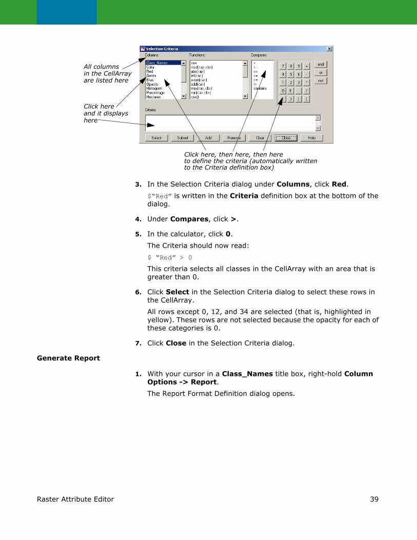
3. In the Selection Criteria dialog under Columns, click Red.
$“Red” is written in the Criteria definition box at the bottom of the dialog.
4. Under Compares, click >.
5. In the calculator, click 0.
The Criteria should now read:
$ “Red” > 0
This criteria selects all classes in the CellArray with an area that is greater than 0.
6. Click Select in the Selection Criteria dialog to select these rows in the CellArray.
All rows except 0, 12, and 34 are selected (that is, highlighted in yellow). These rows are not selected because the opacity for each of these categories is 0.
7. Click Close in the Selection Criteria dialog.
Generate Report
1. With your cursor in a Class_Names title box, right-hold Column Options -> Report.
The Report Format Definition dialog opens.
Click here, then here, then hereto define the criteria (automatically writtento the Criteria definition box)
All columnsin the CellArrayare listed here
Click hereand it displayshere
40 Raster Attribute Editor
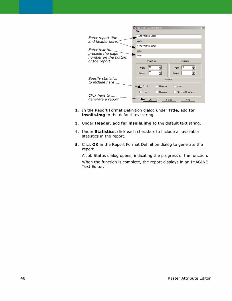
2. In the Report Format Definition dialog under Title, add for lnsoils.img to the default text string.
3. Under Header, add for lnsoils.img to the default text string.
4. Under Statistics, click each checkbox to include all available statistics in the report.
5. Click OK in the Report Format Definition dialog to generate the report.
A Job Status dialog opens, indicating the progress of the function.
When the function is complete, the report displays in an IMAGINE Text Editor.
Click here to generate a report
Enter text to precede the page number on the bottom of the report
Enter report title and header here
Specify statistics to include here
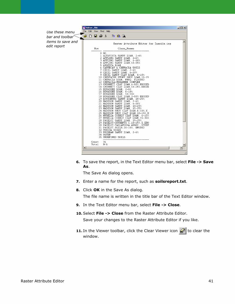
41Raster Attribute Editor
6. To save the report, in the Text Editor menu bar, select File -> Save As.
The Save As dialog opens.
7. Enter a name for the report, such as soilsreport.txt.
8. Click OK in the Save As dialog.
The file name is written in the title bar of the Text Editor window.
9. In the Text Editor menu bar, select File -> Close.
10. Select File -> Close from the Raster Attribute Editor.
Save your changes to the Raster Attribute Editor if you like.
11. In the Viewer toolbar, click the Clear Viewer icon to clear the window.
Use these menubar and toolbar
edit reportitems to save and
42 Profile Tools
Profile Tools The spectral profile display is fundamental to the analysis of hyperspectral data sets. As the number of bands increases and the band widths decrease, the remote sensor is evolving toward the visible/infrared spectrometer. The reflectance (DN) of each band within one (spatial) pixel can be plotted to provide a curve approximating the profile generated by a laboratory scanning spectrometer. This allows estimates of the chemical composition of the material in the pixel. To use this tool, follow the steps below.
Prepare ERDAS IMAGINE should be running and a Viewer should be open.
Display Spectral Profile
1. In the Viewer menu bar, select File -> Open -> Raster Layer.
The Select Layer To Add dialog opens.
2. In the Select Layer To Add dialog, select hyperspectral.img under Filename.
3. Click the Raster Options tab at the top of the dialog.
4. In the Raster Options, click the Fit to Frame checkbox to activate it and then click OK.
The file hyperspectral.img displays in the Viewer.
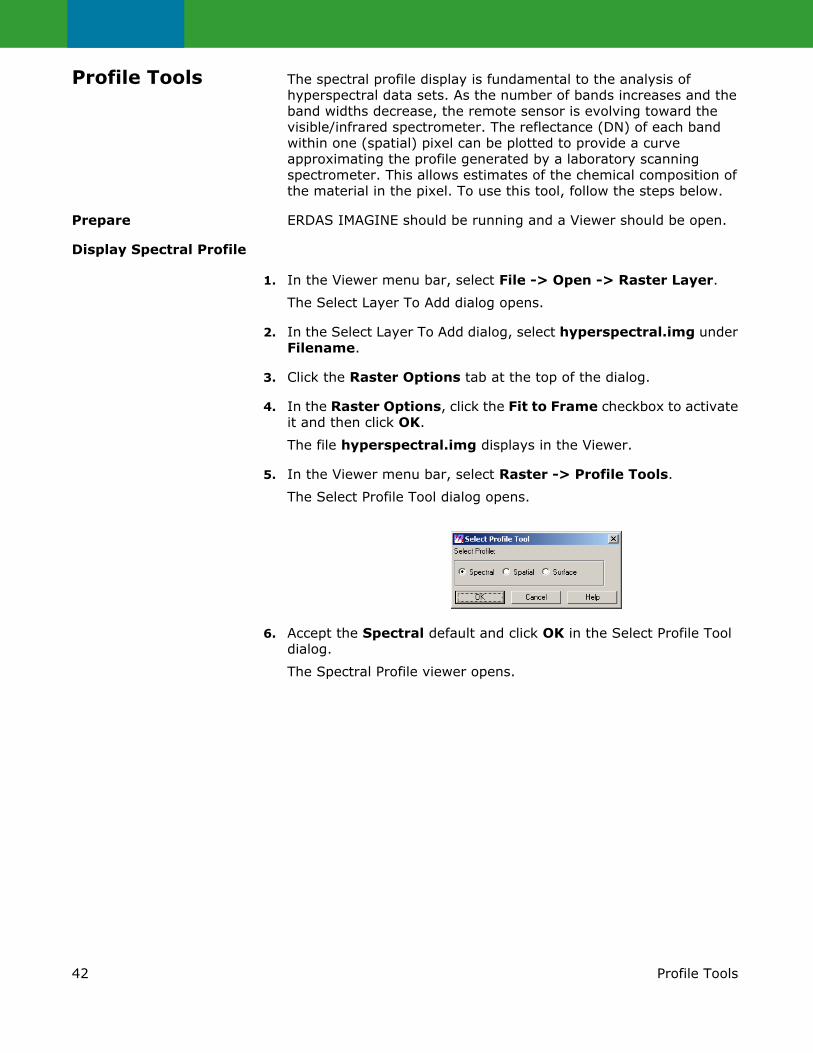
5. In the Viewer menu bar, select Raster -> Profile Tools.
The Select Profile Tool dialog opens.
6. Accept the Spectral default and click OK in the Select Profile Tool dialog.
The Spectral Profile viewer opens.

43Profile Tools
7. In the Spectral Profile viewer, click the Create icon and then select a pixel of interest by clicking it in the Viewer image.
The data for the selected pixel are displayed in the Spectral Profile viewer.
NOTE: The pixel can be moved around the displayed image by dragging it.
Analyze Data
1. In the Spectral Profile viewer menu bar, select Edit -> Chart Options.
The Chart Options dialog opens.
2. In the Chart Options dialog, click the Y Axis tab at the top of the dialog.
3. Set Min to 20 and Max to 180 to control the numerical range.
Click here to create a new profile point in the Viewer
Click this tab to view the options for the Y axis

44 Profile Tools
4. Click Apply and then Close in the Chart Options dialog.
The selected range is shown in detail in the Spectral Profile viewer.
5. In the Spectral Profile viewer menu bar, select Edit -> Plot Stats.
The Spectral Statistics dialog opens.
6. In the Spectral Statistics dialog, change the Window Size to 7.
7. Select Mean and click Apply.
The mean (within the selected window) of Profile 1 is depicted on the graph.
8. Click Cancel in the Spectral Statistics dialog.
9. Select File -> Close from the Spectral Profile viewer.
Display Spatial Profile The Spatial Profile display function allows the analyst to view the reflectance(s) of the pixels along a user-defined polyline. The display can be viewed in either two-dimensional (one band) or perspective three-dimensional (multiple bands) mode. To use this tool, follow the steps below.
The file hyperspectral.img should be displayed in a Viewer, with the Fit to Frame checkbox activated.
1. In the Viewer menu bar, select Raster -> Profile Tools.
The Select Profile Tool dialog opens.
Adjust the window size here
Click to select Mean
Wavelength AxisData tapes containing hyperspectral imagery commonly designate the bands as a simple numerical sequence. When plotted using the profile tools, this yields an x-axis labeled as 1, 2, 3, 4, etc. Elsewhere on the tape or in the accompanying documentation is a file which lists the center frequency and width of each band. This information should be linked to the image intensity values for accurate analysis or comparison to other spectra, such as the Spectra Libraries.
To do this, the band position information must be entered into a linkable format, which is an .saf file. An example of this format can be seen by using a texteditor or vi command to view one of the .saf files in <IMAGINE_HOME>/etc. Once this file is created, it can be linked with the Spectral Profile by using the Edit -> Use Sensor Attributes option.

45Profile Tools
2. Click the Spatial button in the Select Profile Tool dialog and then click OK.
The Spatial Profile viewer opens.
3. Click the Polyline icon in the Spatial Profile viewer toolbar and then draw a polyline on the image in the Viewer. Click to set vertices and middle-click to set an endpoint.
The spatial profile
in the Spatial Profile viewer.
Analyze Data
1. Select Edit -> Plot Layers from the Spatial Profile viewer menu bar.
The Band Combinations dialog opens.
2. Add Layers 2 and 3 to the Layers to Plot column by individually selecting them under Layer and clicking the Add Selected Layer icon
.
3. Click Apply and then Close in the Band Combinations dialog.
Layers 1, 2, and 3 are plotted in the Spatial Profile viewer.
NOTE: Moving the cursor around in the Spatial Profile viewer gives you the pixel values for the x and y coordinates of the layers.
Click here and then here to add the layer to the plot

46 Profile Tools
4. In the Plot Layer box to the right of the toolbar in the Spatial Profile viewer, click the up arrow to view layers 4 and 5.
5. Select Edit -> Plot Layers from the Spatial Profile viewer to again bring up the Band Combinations dialog.
6. In the Band Combinations dialog, click the Add All icon .
7. Click Apply and Close.
As in the Spectral Profile viewer, you can select Edit -> Chart Options to optimize the display.
8. Select File -> Close from the Spatial Profile viewer menu bar.
View Surface Profile The Surface Profile can be used to view any layer (band) or subset in the data cube as a relief surface. To use this tool, follow the steps below.
The file hyperspectral.img should be displayed in a Viewer with the Fit to Frame checkbox activated.
1. In the Viewer menu bar, select Raster -> Profile Tools.
The Select Profile Tool dialog opens.
2. In the Select Profile Tool dialog, click the Surface button and then click OK.
The Surface Profile viewer opens.
3. Click the Rectangle icon in the Surface Profile viewer and then select an AOI in the Viewer by dragging to create a box around it.
When the mouse button is released, the surface profile for the selected area displays in the Surface Profile viewer. As with all of the profile tools, selecting Edit -> Chart Options allows you to optimize the display.
47Image Drape
Analyze Data
It may be desirable to overlay a thematic layer onto this surface. For example, a vegetation map could be overlaid onto a DEM surface, or an iron oxide map (Landsat TM3/TM1) onto a kaolinite peak (1.40 µm) layer. In this example, you overlay a true color image.
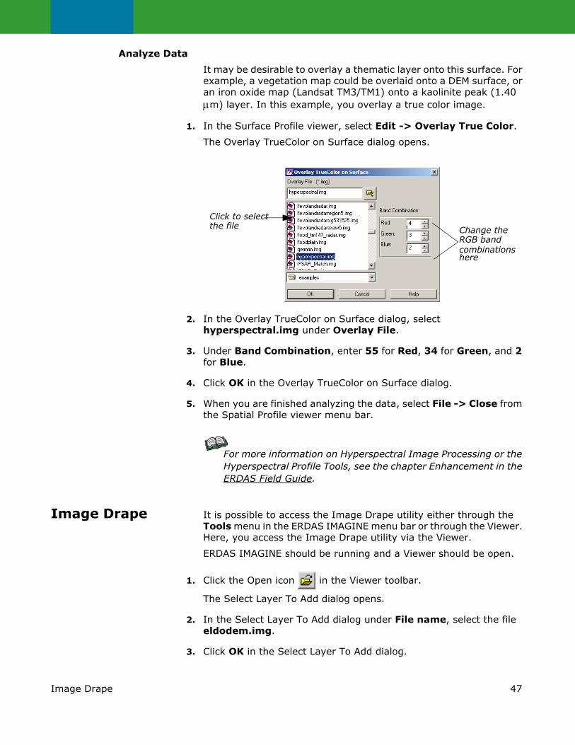
1. In the Surface Profile viewer, select Edit -> Overlay True Color.
The Overlay TrueColor on Surface dialog opens.
2. In the Overlay TrueColor on Surface dialog, select hyperspectral.img under Overlay File.
3. Under Band Combination, enter 55 for Red, 34 for Green, and 2 for Blue.
4. Click OK in the Overlay TrueColor on Surface dialog.
5. When you are finished analyzing the data, select File -> Close from the Spatial Profile viewer menu bar.
For more information on Hyperspectral Image Processing or the Hyperspectral Profile Tools, see the chapter Enhancement in the ERDAS Field Guide.
Image Drape It is possible to access the Image Drape utility either through the Tools menu in the ERDAS IMAGINE menu bar or through the Viewer. Here, you access the Image Drape utility via the Viewer.
ERDAS IMAGINE should be running and a Viewer should be open.
1. Click the Open icon in the Viewer toolbar.
The Select Layer To Add dialog opens.
2. In the Select Layer To Add dialog under File name, select the file eldodem.img.
3. Click OK in the Select Layer To Add dialog.
Click to select the file Change the
RGB band combinations here

48 Image Drape
The file eldodem.img displays in the Viewer.
4. Click the Open icon again in the Viewer toolbar.
The Select Layer To Add dialog reopens.
5. In the Select Layer To Add dialog under File name, select the file eldoatm.img.
6. Click the Raster Options tab at the top of the dialog.
7. In the Raster Options, click the Clear Display checkbox to turn it off. This allows eldoatm.img to display on top of eldodem.img.
8. Click OK in the Select Layer To Add dialog.
Now, both eldodem.img and eldoatm.img are displayed in the same Viewer, with the eldoatm.img layer on top.
9. Select Utility -> Image Drape from the Viewer menu bar.
An Image Drape viewer displays, with the overlapping images in it.
Change Options
1. Select Utility -> Options from the Image Drape viewer menu bar.
The Options dialog opens.
Click this icon to open a file in the Image Drape viewer
Click this icon to open the Observer Positioning tool
Click this icon to open the Sun Positioning tool
49Image Drape
2. Click the Background tab in the Options dialog.
3. In the Background options, hold on the dropdown list next to Background Color and select Gold.
4. Click Apply in the Options dialog.
The background of the image in the Image Drape viewer is now gold.
5. Click Close in the Options dialog.
Change Sun Position
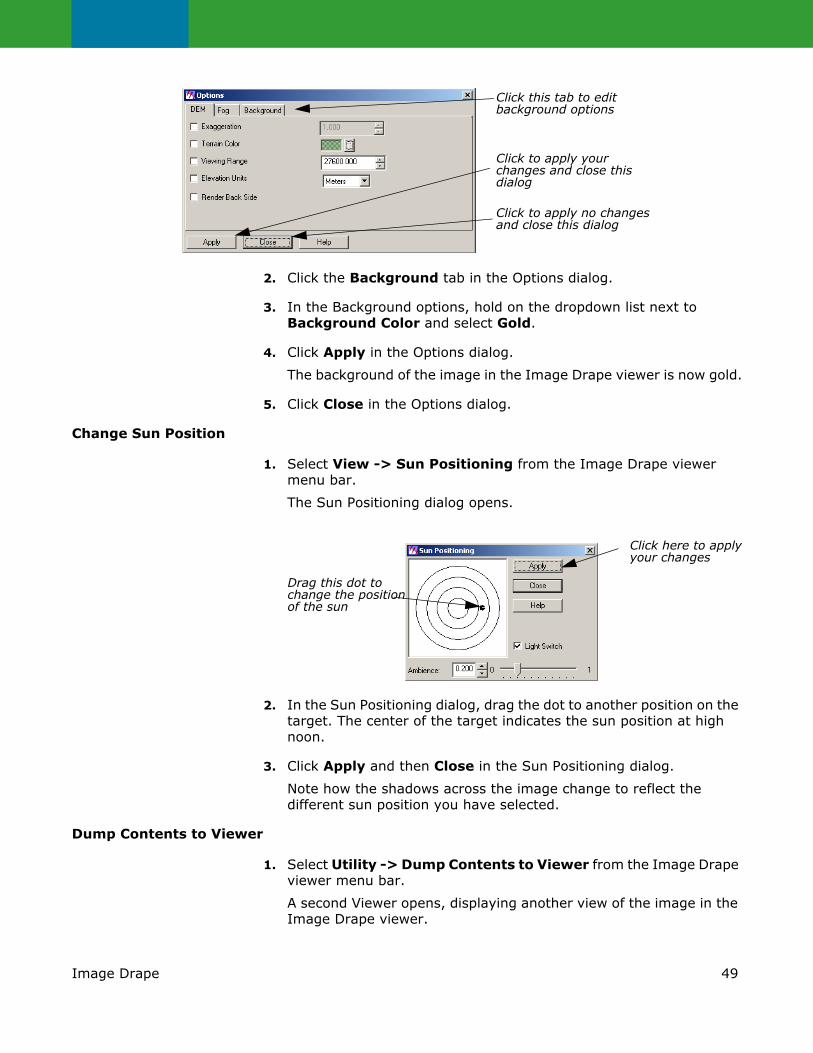
1. Select View -> Sun Positioning from the Image Drape viewer menu bar.
The Sun Positioning dialog opens.
2. In the Sun Positioning dialog, drag the dot to another position on the target. The center of the target indicates the sun position at high noon.
3. Click Apply and then Close in the Sun Positioning dialog.
Note how the shadows across the image change to reflect the different sun position you have selected.
Dump Contents to Viewer
1. Select Utility -> Dump Contents to Viewer from the Image Drape viewer menu bar.
A second Viewer opens, displaying another view of the image in the Image Drape viewer.
Click this tab to editbackground options
Click to apply your changes and close thisdialog
Click to apply no changesand close this dialog
Drag this dot tochange the positionof the sun
Click here to applyyour changes

50 Image Drape
2. Select File -> Close in the first Viewer to clear it from the screen.
3. Select View -> Link/Unlink with Viewer from the Image Drape viewer menu bar.
An instructions box opens, directing you to click in the Viewer to which you want the Image Drape viewer to be linked.
4. Click in the Viewer you just created.
The viewers are now linked and a Positioning tool displays in the Viewer.
NOTE: The bounding box in the Viewer image pictured above is for visual purposes only, and does not actually appear in the Viewer window.
Start Eye/Target
1. To make the Positioning tool easier to see in the Viewer, select Utility -> Selector Properties from the Viewer menu bar.
The Eye/Target Edit dialog opens.
2. In the Eye/Target Edit dialog, hold on the Selector Color dropdown list and select a color that displays well in the Viewer image (for example, Yellow).
The point of observation (“target”)
Positioning tool
The observer’s point- of-view (“eye”)
Hold on this dropdown list to change the selector color

51Image Drape
3. Click OK in the Eye/Target Edit dialog.
The dialog closes and the color of the Positioning tool is updated to the designated color.
Manipulate the Observer and Field of View
You can manipulate the observer and the observer’s field of view in several ways. See step 1 through step 3 below to learn how to obtain different views using the Positioning tool and the Position Parameters dialog.
Use the Positioning Tool
1. Click the Observer Positioning icon in the Image Drape viewer toolbar.
The Position Parameters dialog opens.
2. Drag on the Eye marker of the Positioning tool to change the observer’s point of view in the Image Drape viewer.
The data in the Position Parameters dialog updates to reflect the changes in the observer’s position. The view in the Image Drape viewer is also updated.
If the image in the Image Drape viewer does not completely refresh when the mouse button is released, click the Update icon
.
3. Next, drag on the Target marker of the Positioning tool to change the point of observation in the Image Drape viewer.
The data in the Position Parameters dialog updates to reflect the changes in the point of observation. The view in the Image Drape viewer is also updated.
4. Change the position of both the observer and the target at once by dragging on the line that connects them in the Viewer.
The data in the Position Parameters dialog and the Image Drape viewer is updated.
5. In the Image Drape viewer, click the Goto icon to return to the original position of the observer and the target.
Control ground level positioning here
Control sea level positioning here
Manipulate the Field of View here
52 GLT Viewer
The image and the Positioning tool in the Viewer are updated to their original position. The Position Parameters dialog is also updated.
Use the Position Parameters Dialog
1. In the Position Parameters dialog, change the FOV to 90 and the Roll to 45, then click Apply.
The image in the Image Drape viewer is updated to reflect this change.
2. In the Position Parameters dialog under Observer Position, enter 3000 in the AGL (Above Ground Level) number field.
3. Click Apply and then Close in the Position Parameters dialog.
GLT Viewer The Geospatial Light Table is the optional Viewer available with IMAGINE. The GLT Viewer has a Geospatial Tools palette that can be displayed and hidden as needed. The Geospatial Tools palette aids the visual analyst by providing multiple viewing windows and placing at the fingertips many of the most frequently used geospatial tools. The Geospatial Tools palette also provides enhanced functionality in the status bar below the view panes.
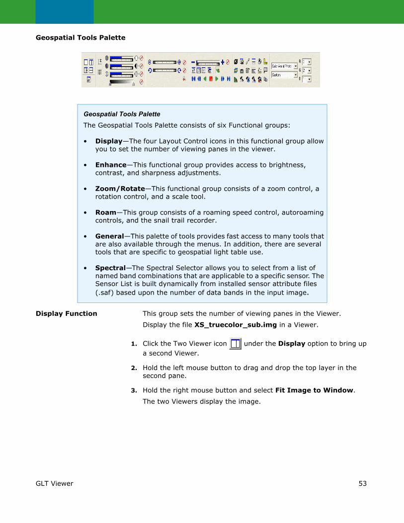
53GLT Viewer
Geospatial Tools Palette
Display Function This group sets the number of viewing panes in the Viewer.
Display the file XS_truecolor_sub.img in a Viewer.
1. Click the Two Viewer icon under the Display option to bring up a second Viewer.
2. Hold the left mouse button to drag and drop the top layer in the second pane.
3. Hold the right mouse button and select Fit Image to Window.
The two Viewers display the image.
Geospatial Tools PaletteThe Geospatial Tools Palette consists of six Functional groups:
• Display—The four Layout Control icons in this functional group allow you to set the number of viewing panes in the viewer.
• Enhance—This functional group provides access to brightness, contrast, and sharpness adjustments.
• Zoom/Rotate—This functional group consists of a zoom control, a rotation control, and a scale tool.
• Roam—This group consists of a roaming speed control, autoroaming controls, and the snail trail recorder.
• General—This palette of tools provides fast access to many tools that are also available through the menus. In addition, there are several tools that are specific to geospatial light table use.
• Spectral—The Spectral Selector allows you to select from a list of named band combinations that are applicable to a specific sensor. The Sensor List is built dynamically from installed sensor attribute files (.saf) based upon the number of data bands in the input image.
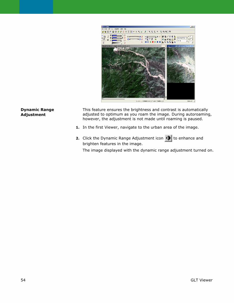
54 GLT Viewer
Dynamic Range Adjustment
This feature ensures the brightness and contrast is automatically adjusted to optimum as you roam the image. During autoroaming, however, the adjustment is not made until roaming is paused.
1. In the first Viewer, navigate to the urban area of the image.
2. Click the Dynamic Range Adjustment icon to enhance and brighten features in the image.
The image displayed with the dynamic range adjustment turned on.
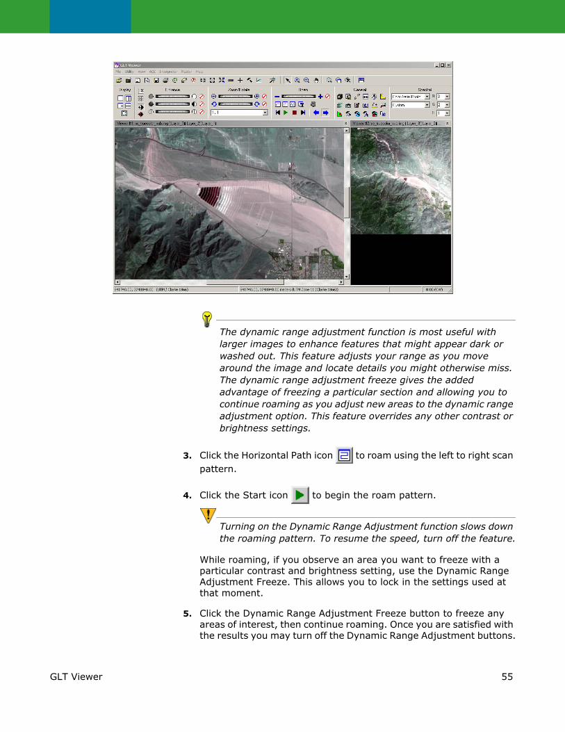
55GLT Viewer
The dynamic range adjustment function is most useful with larger images to enhance features that might appear dark or washed out. This feature adjusts your range as you move around the image and locate details you might otherwise miss. The dynamic range adjustment freeze gives the added advantage of freezing a particular section and allowing you to continue roaming as you adjust new areas to the dynamic range adjustment option. This feature overrides any other contrast or brightness settings.
3. Click the Horizontal Path icon to roam using the left to right scan pattern.
4. Click the Start icon to begin the roam pattern.
Turning on the Dynamic Range Adjustment function slows down the roaming pattern. To resume the speed, turn off the feature.
While roaming, if you observe an area you want to freeze with a particular contrast and brightness setting, use the Dynamic Range Adjustment Freeze. This allows you to lock in the settings used at that moment.
5. Click the Dynamic Range Adjustment Freeze button to freeze any areas of interest, then continue roaming. Once you are satisfied with the results you may turn off the Dynamic Range Adjustment buttons.
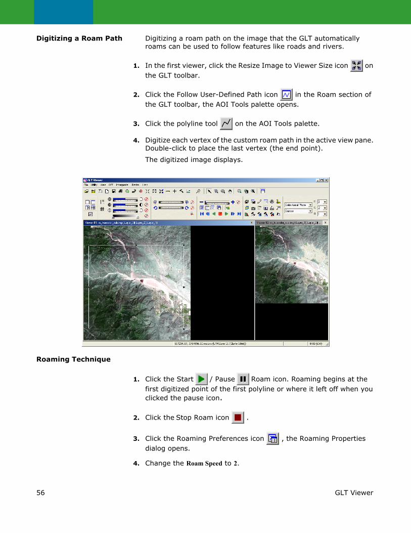
56 GLT Viewer
Digitizing a Roam Path Digitizing a roam path on the image that the GLT automatically roams can be used to follow features like roads and rivers.
1. In the first viewer, click the Resize Image to Viewer Size icon on the GLT toolbar.
2. Click the Follow User-Defined Path icon in the Roam section of the GLT toolbar, the AOI Tools palette opens.
3. Click the polyline tool on the AOI Tools palette.
4. Digitize each vertex of the custom roam path in the active view pane. Double-click to place the last vertex (the end point).
The digitized image displays.
Roaming Technique
1. Click the Start / Pause Roam icon. Roaming begins at the first digitized point of the first polyline or where it left off when you clicked the pause icon.
2. Click the Stop Roam icon .
3. Click the Roaming Preferences icon , the Roaming Properties dialog opens.
4. Change the Roam Speed to 2.

57GLT Viewer
5. Click OK to Close the Roaming Properties dialog.
6. Click the Go to Start icon and click Start again to roam.
Use the AOI Tool palette for other roaming techniques that can be defined. Build a Multiple Point Auto Roam with the point tool, Confine Auto roam to a User-Defined Rectangle/Square with the rectangle tool, or Confine Auto roam to a User-Defined ellipse/circle with the ellipse tool. Once these options are chosen, start roaming using the roaming techniques above.
Create a Snail Trail The Snail Trail is an annotation layer indicating areas of the image over which you have roamed. Only one snail trail may be open at any time. When roaming, the area displayed in the main view pane is represented as a trail of contrasting color over a color block that represents the full extent of the image. The snail trail view pane may also contain any data that includes the extents of the image in the main view pane and that has the same projection (including the same image). To use the snail trail recorder, Viewer #1 must be populated with imagery.
The two Viewers should display the file XS_truecolor_sub.img.
1. Select the second Viewer to record the snail trail.
2. Click the Record Snail Trail icon in the Roam section of the Geospatial Tool Palette to create a new snail trail.
The Snail Trail Menu is added to the GLT Viewer.

58 GLT Viewer
3. Select Snail Trail -> Properties from the GLT Viewer menu.
The Snail Trail Properties menu opens.
4. Click the dropdown list and change the Seen Color to Red.
The current screen to file pixel ratio must be below the threshold set in the Snail Trail Properties dialog.
5. Click OK to close the Snail Trail Properties dialog.
6. Select the main view pane.
7. Click the Horizontal Path roaming technique.
8. Click Play to observe the path left in the snail trail pane (second Viewer).
9. Pause the path of the snail trail by clicking the Pause button. To start again, click the Play button.
The snail trail pauses in the second Viewer.

59GLT Viewer
10. Click the snail trail view pane to activate it.
11. Click the Save icon to save the snail trail path.