CONVERGENCE ANALYSIS FOR ANDERSON ACCELERATION

ALEX TOTH∗ AND C. T. KELLEY ∗

Abstract. Anderson(m) is a method for acceleration of fixed point iteration which stores m + 1 priorevaluations of the fixed point map and computes the new iteration as a linear combination of those evalu-ations. Anderson(0) is fixed point iteration. In this paper we show that Anderson(m) is locally r-linearlyconvergent if the fixed point map is a contraction and the coefficients in the linear combination remainbounded. We prove q-linear convergence of the residuals for linear problems for Anderson(1) without theassumption of boundedness of the coefficients. We observe that the optimization problem for the coefficientscan be formulated and solved in non-standard ways and report on numerical experiments which illustratethe ideas.

Key words. Nonlinear Equations, Anderson acceleration, Local convergence

AMS subject classifications. 65H10,

1. Introduction. Anderson acceleration (also known as Anderson mixing) [1], is essen-tially the same as Pulay mixing (also known as Direct Inversion on the Iterative Subspace, orDIIS) [22,28–30,32] and the nonlinear GMRES method [4,23,25,34]. The method has beenwidely used to accelerate the SCF iteration in electronic structure computations. Recentpapers [27, 30, 31, 33] show that the method is related to multisecant quasi-Newton methodor, in the case of linear problems, GMRES. None of these results lead to a convergence proof,even in the linear case, unless the available storage is large enough to allow GMRES to takea number of iterations equal to the dimension of the problem. Anderson acceleration doesnot require the computation or approximation of Jacobians or Jacobian-vector products, andthis can be an advantage over Newton-like methods.

Anderson acceleration is a method for solving fixed point problems

u = G(u),(1.1)

where u ∈ RN and G : RN → RN . In this paper we prove that Anderson iteration convergeswhen G is a contraction, which implies that the conventional fixed point iteration

uk+1 = G(uk)(1.2)

also converges. In the linear case we show that the convergence rate is no worse that fixedpoint iteration. In the nonlinear case we we show that, in a certain sense, the convergencespeed can be made as close to the speed of fixed point iteration as one likes, provided theinitial iterate is sufficiently near a solution and the coefficients {αkj} (defined below) in theiteration remain bounded.

∗North Carolina State University, Department of Mathematics, Box 8205, Raleigh, NC 27695-8205, USA(Tim Kelley@ncsu.edu,artoth@ncsu.edu). The work of these authors has been partially supported by theConsortium for Advanced Simulation of Light Water Reactors (www.casl.gov), an Energy Innovation Hub(http://www.energy.gov/hubs) for Modeling and Simulation of Nuclear Reactors under U.S. Departmentof Energy Contract No. DE-AC05-00OR22725, National Science Foundation Grants CDI-0941253, OCI-0749320, and SI2-SSE-1339844, and Army Research Office Grants W911NF-11-1-0367, and W911NF-07-1-0112.

1

CASL-U-2014-0226-000

2 Toth, Kelley

The Anderson iteration maintains a history of residuals

F (u) = G(u)− u

of depth at most m + 1, where m is an algorithmic parameter. When m is important, wewill call the iteration Anderson(m). Anderson(0) is fixed point iteration by definition.

A formal algorithmic description is

anderson(u0, G,m)

u1 = G(u0); F0 = G(u0)− u0for k = 1, . . . domk = min(m, k)Fk = G(uk)− ukMinimize ‖∑mk

j=0 αkjFk−mk+j‖ subject to∑mk

j=0 αkj = 1.

uk+1 = (1− βk)∑mkj=0 α

kjuk−mk+j + βk

∑mkj=0 α

kjG(uk−mk+j)

end for

One could use any norm in the minimization step, as we will see § 2. Typically oneuses the `2 norm, so the minimization problem can be formulated as a linear least squaresproblem [33] and solved easily. In this approach we solve the unconstrained problem

min ‖F (uk)−mk∑j=1

αkj (F (uk−mk+j)− F (uk))‖2,(1.3)

for {αkj}kj=1. Then we recover αk0 by

αk0 = 1−mk∑j=1

αkj .

This formulation of the linear least squares problem is not optimal for implementation, apoint we discuss in more detail in § 3. Our analysis uses (1.3) because it explicitly displaysthe coefficients {αkj}.

If one uses the `1 or `∞ norms, the optimization problem can be expressed as a linearprogram [13], for which there are many efficient solvers.

The mixing parameters {βk} are generally determined heuristically. For this discussionwe will set βk ≡ 1. If G is linear, one can show that uk+1 is a linear combination of priorresiduals. This implies [33] that uk+1 = G(uGMRES

k ) for k ≤ m, if I − G is nonsingular,as long as the linear residuals are strictly decreasing. In particular, if m > N , G is linear,I −G is nonsingular, and the residuals strictly decrease, then the iteration will converge tothe solution. However, even in the linear case [27], the Anderson iterations can stagnate atan incorrect result. In the nonlinear case [12, 30] one can show that, for m ≤ N , Andersoniteration is a multisecant method, but there is no convergence theory for such methods.

CASL-U-2014-0226-000

Anderson Acceleration 3

In most applications m is small. m = 1 or m = 2 is common for large electronic structurecomputations [2]. In these cases (large N and small m) there are no convergence results evenin the linear case.

In this paper we prove three convergence results for Anderson acceleration when appliedto contractive mappings. We prove that the residuals converge q-linearly for linear problemsin § 2.1 and, in § 2.3, under certain conditions when m = 1. In the general nonlinearcase we prove local r-linear convergence in § 2.2 under the assumption that the coefficients{αkj} remain bounded. All our results remain valid in an infinite-dimensional Banach spacesetting, provided one can solve the optimization problem for the coefficients.

2. Convergence. In this section we prove three convergence theorems. In the linearcase the convergence of the residuals is q-linear. Recall that a sequence {wk} convergesq-linearly with q-factor c ∈ [0, 1) to w∗ if

‖wk+1 − w∗‖ ≤ c‖wk − w∗‖

for all k ≥ 0. In the nonlinear case the convergence of the residuals is r-linear. This meansthat there is c ∈ (0, 1) and M > 0 such that

‖wk − w∗‖ ≤Mck‖w0 − w∗‖.

In both cases, the convergence of uk to the solution is r-linear.Finally, in Theorem 2.4 we prove q-linear convergence of the Anderson(1) residuals to

zero when the optimization is done in the `2 norm. Note that, [9,16], if the residuals, eitherlinear or nonlinear, converge to q-linearly to zero, then the errors converge q-linearly to zeroin the norm ‖ · ‖∗, which is defined by

‖w‖∗ = ‖F ′(u∗)w‖.

All of the proofs depend on the fact that if {αj}mkj=0 is the solution of the least squaresproblem at iteration k, then by definition

‖mk∑j=0

αjF (uk−mk+j)‖ ≤ ‖F (uk)‖.(2.1)

2.1. Linear Problems. In this section M is a linear operator with ‖M‖ = c < 1. Weconsider the linear fixed-point problem

u = G(u) ≡Mu+ b.

The residual in this case is

F (u) = G(u)− u = b− (I −M)u.

Theorem 2.1. If ‖M‖ = c < 1, then the Anderson iteration converges to u∗ =(I −M)−1b and the residuals converge q-linearly to zero with q-factor c.

CASL-U-2014-0226-000

4 Toth, Kelley

Proof. Since∑αj = 1, the new residual is

F (uk+1) = b− (I −M)uk+1 =∑mkj=0 αj [b− (I −M)(b+Muk−mk+j)]

=∑mkj=0 αjM [b− (I −M)uk−mk+j] = M

∑mkj=0 αjF (uk−mk+j)

Hence, by (2.1)

‖F (uk+1)‖ ≤ c‖F (uk)‖,

as asserted.If we set e = u − u∗, then F (u) = −(I − M)e. So q-linear convergence of residuals

implies that

(1− c)‖ek‖ ≤ ‖F (uk)‖ ≤ ck‖F (u0)‖ ≤ ck(1 + c)‖e0‖

and hence

‖ek‖ ≤(

1 + c

1− c

)ck‖e0‖.

which is r-linear convergence with r-factor c.

2.2. Nonlinear Problems and Local r-linear Convergence. In this section weprove a local r-linear convergence result. Our result applies to any iteration of the form

uk+1 =mk∑j=0

αkjG(uk−mk+j),(2.2)

for a fixed m and mk = min(m, k) if the coefficients αkj satisfy Assumption 2.1.Assumption 2.1.1. ‖∑mk

j=0 αjF (uk−mk+j)‖ ≤ ‖F (uk)‖ (which is (2.1)) holds,2.∑mkj=0 αj = 1, and

3. There is Mα such that for all k ≥ 0∑mkj=1 |αj| ≤Mα.

The first two parts of Assumption 2.1 are trivially satisfied by Anderson acceleration.The boundedness requirement in the third part would follow, for example, from uniformwell-conditioning of the `2 nonlinear least squares problem (1.3), which, as [33] observes, isnot guaranteed. In fact, as we show by example in § 3, the least squares problem can becomehighly ill-conditioned while the coefficients still remain bounded. We have not seen a case inour testing where the coefficients become large, but we are not able to prove that they remainbounded, hence the assumption. A method to modify mk in response to ill-conditioning wasproposed in [33]. We propose to address the boundedness of the coefficients directly.

One can modify Anderson acceleration to enforce boundedness of the coefficients by, forexample,

• restarting the iteration when the coefficients exceed a threshold,• imposing a bound constraint on the linear least squares problem and solving that

problem with the method of [6], or• minimizing in `1 or `∞, adding the bound as a constraint, and formulating the result-

ing problem as a linear program.

CASL-U-2014-0226-000

Anderson Acceleration 5

The first of these is by far the simpler and, based on our experience, is unlikely to changethe iteration at all.

The assumptions we make on the nonlinearity G and the solution u∗, Assumption 2.2implies the usual standard assumptions [10,16,26] for local convergence of Newton’s method.As is standard we will let F ′ denote the Jacobian of F and e = u− u∗.

Assumption 2.2.• There is u∗ ∈ RN such that F (u∗) = G(u∗)− u∗ = 0.• G is Lipschitz continuously differentiable in the ball B(ρ) = {u | ‖e‖ ≤ ρ} for someρ > 0.• There is c ∈ (0, 1) such that for all u, v ∈ B(ρ), ‖G(u)−G(v)‖ ≤ c‖u− v‖.The last of these assumptions implies that ‖G′(u)‖ ≤ c < 1 for all u ∈ B(ρ), and hence

F ′(u∗) is nonsingular. We will let G∗ = G′(u∗). We will need a special case of a result(Lemma 4.3.1) from [16]. We will denote the Lipschitz constant of F ′ in B(ρ) by γ.

Lemma 2.2. For ρ ≤ ρ sufficiently small and all u ∈ B(ρ),

‖F (u)− F ′(u∗)e‖ ≤ γ

2‖e‖2(2.3)

and‖e‖(1− c) ≤ ‖F (u)‖ ≤ (1 + c)‖e‖.(2.4)

Theorem 2.3. Let Assumption 2.2 hold and let c < c < 1. Then if u0 is sufficientlyclose to u∗, the Anderson iteration converges to u∗ r-linearly with r-factor no greater thanc. In fact

‖F (uk)‖ ≤ ck‖F (u0)‖(2.5)

and

‖ek‖ ≤(1 + c)

1− cck‖e0‖.(2.6)

Proof. We let u0 ∈ B(ρ) and assume that ρ ≤ ρ, where ρ is from the statement ofLemma 2.2. We will prove (2.5). (2.6) will follow from (2.5) and Lemma 2.2.

Reduce ρ if needed so that ρ < 2(1− c)/γ and(cc

+(Mαγρ2(1−c)

)c−m−1

)(1− γρ

2(1−c)

) ≤ 1.(2.7)

Now reduce ‖e0‖ further so that(Mα(c+ γρ/2)

1− c

)c−m‖F (u0)‖ ≤

(Mα(1 + c)(c+ γρ/2)

1− c

)c−m‖e0‖ ≤ ρ.(2.8)

We will proceed by induction. Assume that for all 0 ≤ k ≤ K that

‖F (uk)‖ ≤ ck‖F (u0)‖,(2.9)

CASL-U-2014-0226-000

6 Toth, Kelley

which clearly holds for K = 0.Equations (2.8) and (2.9) imply that ‖ek‖ ≤ ρ for 1 ≤ k ≤ K. Hence, by (2.3)

F (uk) = F ′(u∗)ek + ∆k

where,

‖∆k‖ ≤γ

2‖ek‖2.(2.10)

This implies thatG(uk) = u∗ +G∗ek + ∆k.(2.11)

By (2.11) and the fact that∑αKj = 1,

uK+1 = u∗ +∑mKj=0 α

Kj (G∗eK−mK+j + ∆K−mK+j)

= u∗ +∑mKj=0(α

Kj G

∗eK−mK+j) + ∆K

(2.12)

where

∆K =mK∑j=0

αKj ∆K−mK+j.

Our next task is to estimate ∆K . (2.10) and (2.12) imply that

‖∆K‖ =mK∑j=0

|αKj |γ‖eK−mK+j‖2/2.(2.13)

Lemma 2.2, the induction hypothesis, and the fact that

K −mK + j = K −min(m,K) + j ≥ K −m,

imply that

‖eK−mK+j‖2 ≤ ‖eK−mK+j‖(

11−c

)‖F (uK−mK+j)‖ ≤

(ρ

1−c

)‖F (uK−mK+j)‖

≤(

ρ1−c

)c(K−mK+j)‖F (u0)‖ ≤

(ρ

1−c

)cK−m‖F (u0)‖.

(2.14)

So, since∑ |αKj | ≤Mα, we have

‖∆K‖ ≤(Mαγρ

2(1− c)

)cK−m‖F (u0)‖ ≤

(Mαγρ

2(1− c)

)c−m‖F (u0)‖.(2.15)

Write (2.12) as

eK+1 =mK∑j=0

(αKj G∗eK−mK+j) + ∆K .

The induction hypothesis implies that, for 0 ≤ j ≤ mk,

‖eK−mK+j‖ ≤(

11−c

)‖F (uK−mK+j)‖

≤(

11−c

)cK−mK+j‖F (u0)‖ ≤

(1

1−c

)c−m‖F (u0)‖,

CASL-U-2014-0226-000

Anderson Acceleration 7

and hence

‖mK∑j=0

(αKj G∗eK−mK+j)‖ ≤

(Mαc

1− c

)c−m‖F (u0)‖.(2.16)

Combining (2.11), (2.15), and (2.16) yields

‖eK+1‖ ≤ ‖F (u0)‖(Mα(c+ γρ/2)

1− c

)c−m ≤ ρ,

by (2.8).Since ‖eK+1‖ ≤ ρ ≤ ρ, we may apply (2.11) with k = K + 1 to obtain,

F (uK+1) = (G∗ − I)eK+1 + ∆K+1

where, by Lemma 2.2,

‖∆K+1‖ ≤γ

2‖eK+1‖2.

So, since G∗ and G∗ − I commute,

F (uK+1) = G∗∑mKj=0(α

Kj (G∗ − I)eK−mK+j) + (G∗ − I)∆K + ∆K+1

= G∗∑mKj=0(α

Kj F (uK−mK+j)− αKj ∆K−mK+j) + (G∗ − I)∆K + ∆K+1

= G∗∑mKj=0(α

Kj F (uK−mK+j))− ∆K + ∆K+1.

(2.17)

Combine (2.17) with (2.4) to obtain,

‖∆K+1‖ ≤(

γ

2(1− c)

)ρ‖F (uK+1)‖(2.18)

The induction hypothesis, (2.1), (2.15), (2.17), and (2.18) imply that

‖F (uK+1)‖(1− γρ

2(1−c)

)≤ ‖F (uK+1)‖ − ‖∆K+1‖

≤ c‖∑mKj=0 α

Kj F (uK−mK+j)‖+ ‖∆K‖

≤ c‖F (uK)‖+ ‖∆K‖

=(cc

+(Mαγρ2(1−c)

)c−m−1

)cK+1‖F (u0)‖

(2.19)

Therefore

‖F (uK+1)‖ ≤

(cc

+(Mαγρ2(1−c)

)c−m−1

)(1− γρ

2(1−c)

) cK+1‖F (u0)‖ ≤ cK+1‖F (u0)‖

since (cc

+(Mαγρ2(1−c)

)c−m−1

)(1− γρ

2(1−c)

) ≤ 1,

by (2.7). This completes the proof.

CASL-U-2014-0226-000

8 Toth, Kelley

2.3. Convergence for Anderson(1). In this section we prove convergence for Ander-son(1) with the `2 norm. We will assume that Assumption 2.2 holds. We show directly thatthe coefficients are bounded if c is sufficiently small and prove q-linear convergence of theresiduals in that case. The analysis here is quite different from the Anderson(m) case inthe previous section, depending heavily on both m = 1 and the fact that the optimizationproblem for the coefficients is a linear least squares problem.

We will express the iteration as

uk+1 = (1− αk)G(uk) + αkG(uk−1),(2.20)

and note that

αk =F (uk)

T (F (uk)− F (uk−1))

‖F (uk)− F (uk−1)‖2(2.21)

Theorem 2.4. Assume that Assumption 2.2 holds, that u0 ∈ B(ρ), and that c is smallenough so that

c ≡ 3c− c2

1− c< 1.(2.22)

Then the Anderson(1) residuals with `2 optimization residuals converge q-linearly with q-factor c.

Proof. We induct on k. Assume that

‖F (uk)‖ ≤ c‖F (uk−1)‖(2.23)

for all 0 ≤ k ≤ K. (2.23) is trivially true for K = 1, since Anderson(0) is successivesubstitution and c < c.

Now defineAk = G(uk+1)−G((1− αk)uk + αkuk−1)

andBk = G((1− αk)uk + αkuk−1)− uk+1.

ClearlyF (uK+1) = G(uK+1)− uK+1 = AK +BK .(2.24)

We will obtain an estimate of F (uK+1) by estimating AK and BK separately.By definition of the Anderson iteration (2.20) and contractivity of G

‖AK‖ = ‖G(uK+1)−G((1− αK)uK + αKuK−1)‖

≤ c‖uK+1 − (1− αK)uK − αKuK−1‖

= c‖(1− αK)(G(uK)− uK)− αK(G(uK−1)− uK−1)‖

= c‖(1− αK)F (uK)− αKF (uK−1)‖ ≤ c‖F (uK)‖,

(2.25)

where the last inequality follows from the optimality property of the coefficients.

CASL-U-2014-0226-000

Anderson Acceleration 9

Now letδK = uK−1 − uK .

To estimate BK we note that

BK = G((1− αK)uK + αKuK−1)− (1− αK)G(uK)− αKG(uK−1)

= G(uK + αKδK)−G(uK) + αK(G(uK)−G(uK−1))

=∫ 10 G

′(uK + tαKδK)αKδK dt− αK∫ 10 G

′(uK + tδK)δK dt

= αK∫ 10

[G′(uK + tαKδK)−G′(uK + tδK)

]δK dt.

(2.26)

This leads to the estimate

‖BK‖ ≤ |αK |‖δK‖∫ 10 ‖G′(uK + tαKδK)−G′(uK + tδK)‖ dt ≤ 2c|αK |‖δK‖(2.27)

The next step is to estimate αK . The difference in residuals is

F (uK)− F (uK−1) = G(uK)−G(uK−1) + δK = δK −∫ 10 G

′(uK−1 − tδK)δK dt

= (I −∫ 10 G

′(uK−1 − tδK) dt)δK

Since ‖G′(u)‖ ≤ c for all u ∈ B(ρ) we have

‖δK‖ ≤ ‖F (uK)− F (uK−1)‖/(1− c).(2.28)

Combine (2.28) and (2.21) to obtain

|αK |‖δK‖ ≤‖F (uK)‖

‖F (uK)− F (uK−1)‖‖δK‖ ≤

‖F (uK)‖1− c

.(2.29)

Now, we combine (2.25), (2.27), and (2.29) to obtain

‖F (uK+1)‖‖F (uK)‖

≤ c+2c

1− c= c.(2.30)

Our assumption that c < 1 completes the proof.Note that q-linear convergence of the residuals implies that the coefficients are bounded

because

|αK | ≤ ‖F (uK)‖‖F (uK)− F (uK−1)‖

≤ c‖F (uK−1)‖‖F (uK−1)‖(1− c)

≤ c

1− c.

For sufficiently good initial data, one can use the proof of Theorem 2.4 to prove q-linearconvergence for all c ∈ [0, 1).

Corollary 2.5. Assume that Assumption 2.2 holds and that c ∈ (c, 1). Then if ‖e0‖is sufficiently small, the Anderson(1) residuals with `2 optimization converge q-linearly withq-factor no larger than c. Moreover

lim supk→∞

‖F (uk+1)‖‖F (uk)‖

≤ c.(2.31)

CASL-U-2014-0226-000

10 Toth, Kelley

Proof. We use the standard assumptions, (2.21), and (2.26) to estimate BK . Note that1 + γ is an upper bound for the Lipschitz constant of G′. Equations (2.21) and (2.26) implythat

‖BK‖ ≤(1 + γ)|αK ||1− αK |‖δK‖2

2≤ (1 + γ)‖F (uK)‖‖F (uK−1)‖‖δK‖2

2‖F (uK)− F (uK−1)‖2.

Equation (2.28) implies that

‖F (uK)− F (uK−1)‖‖δK‖

≥ (1− c),

and hence

‖BK‖ ≤(1 + γ)‖F (uK−1)‖‖F (uK)‖

2(1− c)2.

Therefore, we can use (2.24) and (2.25) to obtain

‖F (uK+1)‖‖F (uK)‖

≤ c+(1 + γ)‖F (uK−1)‖

2(1− c)2.(2.32)

The right side of (2.32) is ≤ c for all K ≥ 1 if ‖e0‖ is sufficiently small. In that case, theresiduals converge to zero, and (2.31) follows.

3. Numerical Experiments. In this section we report on some simple numerical ex-periments. We implement Anderson acceleration using the approach from [12,21,33], whichis equivalent to (1.3), but organizes the computation to make the coefficient matrix easy toupdate by adding a single column and deleting another. This makes it possible to use fastmethods to update the QR factorization [14] to solve the sequence of linear least squaresproblems if one does the optimization in the `2 norm. According to [33] and our own expe-rience, this form has modestly better conditioning properties.

For the kth iteration we solve

minθ∈Rmk

‖F (uk)−mk−1∑j=0

θj(F (uj+1)− F (uj))‖(3.1)

to obtain a vector θk ∈ Rmk . Then the next iteration is

uk+1 = G(uk)−mk−1∑j=0

θkj (G(uj+1)−G(uj)).(3.2)

In terms of (1.3),

α0 = θ0, αj = θj − θj−1 for 1 ≤ j ≤ mk − 1 and αmk = 1− θmk−1.

CASL-U-2014-0226-000

Anderson Acceleration 11

3.1. Conditioning. Suppose G : R2 → R2,

G(u) =

(g(u1, u2)g(u1, u2)

)

and

u0 =

(ww

).

Then Anderson(2), using the `2 norm may fail because the linear least squares problem willbe rank-deficient. One could, of course, take the minimum norm solution with no ill effects.

Now consider a perturbation of such a problem. The linear least squares problem willbe ill-conditioned, but the size of the coefficients for Anderson(2) may remain bounded. Weillustrate this with a simple example.

Let

G(u) =

(cos((u1 + u2)/2)cos((u1 + u2)/2) + 10−8 sin(u21)

)

We applied Anderson acceleration to this problem with an initial iterate u = (1, 1)T . InTable 3.1 we tabulate the residual norms, the condition number of the coefficient matrixfor the optimization problem for the coefficients, and the `1 norm of the coefficients. Weterminate the iteration when the residual norm falls below 10−10. As one can see, thecondition number becomes very large with little effect on the coefficient norm. We will seea similar effect for the more interesting problem in § 3.2.

Table 3.1Iteration statistics for Anderson(2)

k Residual norm Condition number Coefficient norm0 6.501e-011 4.487e-01 1.000e+00 1.000e+002 2.615e-02 2.016e+10 4.617e+003 7.254e-02 1.378e+09 2.157e+004 1.531e-04 3.613e+10 1.184e+005 1.185e-05 2.549e+11 1.000e+006 1.825e-08 3.677e+10 1.002e+007 1.048e-13 1.574e+11 1.092e+00

3.2. Using the `1 and `∞ norms. In this section we compare the use of Andersonacceleration with the `1, `2, and `∞ norms with a fixed point iteration (Anderson(0)) anda Newton-Krylov iteration. We use the nsoli.m Matlab code from [16, 17] for the Newton-Krylov code and solve the linear programs for the `1 and `∞ optimization problems for thecoefficients with the CVX Matlab software [7, 15]. We used the SeDuMi solver and set theprecision in cvx to high. The `1 and `∞ optimizations are significantly more costly thanthe `2 optimization. While the iteration with the `1 optimization seems to perform well, one

CASL-U-2014-0226-000

12 Toth, Kelley

would need a special-purpose linear programming code tuned for this application to makethat approach practical.

As an example we take the composite midpoint rule discretization of the ChandrasekharH-equation [3, 5]

H(µ) = G(H) ≡(

1− ω

2

∫ 1

0

µ

µ+ νH(ν) dν.

)−1(3.3)

In (3.3) ω ∈ [0, 1] is a parameter and one seeks a solution H∗ ∈ C[0, 1]. The solutionH∗(µ) ≥ 1 satisfies

‖H∗‖∞ ≤ min

(3,

1√1− ω

),

and is an increasing function of µ and ω. This fact and a monoticity argument can be usedto show that if ε > 0 is sufficiently small and u and v are in B(ε)

‖G(u)−G(v)‖ ≤ (1 + ε)2‖H∗‖2∞ω2

‖u− v‖,

for any Lp norm. This inequality also carries over to the discrete problems. In particular, Gis a local contraction for ω = .5, which is one of our test cases.

It is known [18,24], both for the continuous problem and its midpoint rule discretization,that, if ω < 1,

ρ(G′(H∗)) ≤ 1−√

1− ω < 1,

where ρ denotes spectral radius. Hence the local convergence theory in § 2.2 and 2.3 appliesfor some choice of norm. It is also known that if the initial iterate is nonnegative andcomponent-wise smaller than H, then fixed point iteration will converge with a q-factor nolarger than ω. For ω = 1 the nonlinear equation is singular, but both fixed point iterationand Newton-GMRES will converge from our choice of initial iterate [18–20].

For integral equations problems such as this one, where preconditioning is not necessary,Newton-GMRES will be faster than a conventional approach in which one constructs, stores,and factors a Jacobian matrix. Newton-GMRES will converge to truncation error at a costproportional to the square of the size of the spatial grid, whereas the cost of even onefactorization will be cubic. However, for this problem G′ is a compact operator, whichimplies that the coefficient matrix for the optimization problem for the coefficients couldbecome ill-conditioned as the iteration converges, as we see in the tables below.

We report on computational results with an N = 500 point composite midpoint rulediscretization. We compare Anderson(m) for m = 0, . . . , 6 and the `1, `2, and `∞ normswith a Newton-GMRES iteration. The Newton-GMRES iteration used a reduction factorof .1 for the linear residual with each Newton step. Other approaches to the linear solver,such as the one from [11] performed similarly. We terminate the nonlinear iterations when‖F (uk)‖2/‖F (u0)‖2 ≤ 10−8.

We consider values of ω = .5, .99, 1.0, with the last value being one for which F ′ issingular at the solution and ρ(G(H∗)) = 1. When ω = 1,Newton’s method will be linearlyconvergent [8, 20]. One can see this in Table 3.2 by the increase in the number of functioncalls for ω = 1. The initial iteration was (1, 1, . . . , 1)T for all cases. This is a good initialiterate for ω = .5 and a marginal one for the other two cases.

CASL-U-2014-0226-000

Anderson Acceleration 13

In the tables we use function calls as a measure of cost. This is an imperfect metric andthe comparisons should be viewed as qualitative. The cost of the `1 and `∞ optimizations aremore than solving the `2 least squares problem, and we have ignored the orthogonalizationcost within Newton-GMRES. For large problems where the evaluation of G is costly, thecost of the linear program solve should be relatively low, especially for small value of m.

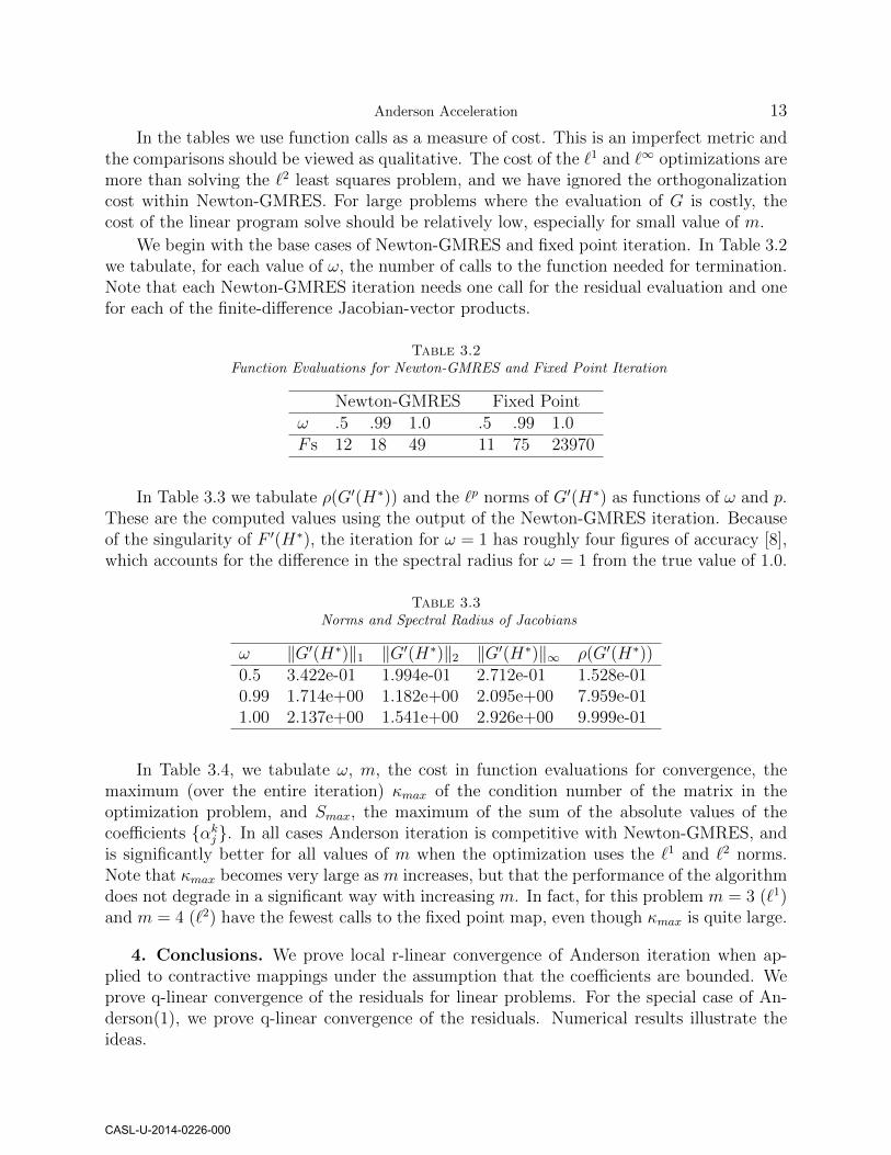
We begin with the base cases of Newton-GMRES and fixed point iteration. In Table 3.2we tabulate, for each value of ω, the number of calls to the function needed for termination.Note that each Newton-GMRES iteration needs one call for the residual evaluation and onefor each of the finite-difference Jacobian-vector products.

Table 3.2Function Evaluations for Newton-GMRES and Fixed Point Iteration

Newton-GMRES Fixed Pointω .5 .99 1.0 .5 .99 1.0F s 12 18 49 11 75 23970

In Table 3.3 we tabulate ρ(G′(H∗)) and the `p norms of G′(H∗) as functions of ω and p.These are the computed values using the output of the Newton-GMRES iteration. Becauseof the singularity of F ′(H∗), the iteration for ω = 1 has roughly four figures of accuracy [8],which accounts for the difference in the spectral radius for ω = 1 from the true value of 1.0.

Table 3.3Norms and Spectral Radius of Jacobians

ω ‖G′(H∗)‖1 ‖G′(H∗)‖2 ‖G′(H∗)‖∞ ρ(G′(H∗))0.5 3.422e-01 1.994e-01 2.712e-01 1.528e-010.99 1.714e+00 1.182e+00 2.095e+00 7.959e-011.00 2.137e+00 1.541e+00 2.926e+00 9.999e-01

In Table 3.4, we tabulate ω, m, the cost in function evaluations for convergence, themaximum (over the entire iteration) κmax of the condition number of the matrix in theoptimization problem, and Smax, the maximum of the sum of the absolute values of thecoefficients {αkj}. In all cases Anderson iteration is competitive with Newton-GMRES, andis significantly better for all values of m when the optimization uses the `1 and `2 norms.Note that κmax becomes very large as m increases, but that the performance of the algorithmdoes not degrade in a significant way with increasing m. In fact, for this problem m = 3 (`1)and m = 4 (`2) have the fewest calls to the fixed point map, even though κmax is quite large.

4. Conclusions. We prove local r-linear convergence of Anderson iteration when ap-plied to contractive mappings under the assumption that the coefficients are bounded. Weprove q-linear convergence of the residuals for linear problems. For the special case of An-derson(1), we prove q-linear convergence of the residuals. Numerical results illustrate theideas.

CASL-U-2014-0226-000

14 Toth, Kelley

Table 3.4Anderson Iteration for H-equation

`1 Optimization `2 Optimization `∞ Optimizationω m F s κmax Smax F s κmax Smax F s κmax Smax0.50 1 7 1.00e+00 1.4 7 1.00e+00 1.4 7 1.00e+00 1.50.99 1 11 1.00e+00 3.5 11 1.00e+00 4.0 10 1.00e+00 10.11.00 1 21 1.00e+00 3.0 21 1.00e+00 3.0 19 1.00e+00 4.80.50 2 6 1.36e+03 1.4 6 2.90e+03 1.4 6 2.24e+04 1.40.99 2 10 1.19e+04 5.2 10 9.81e+03 5.4 10 4.34e+02 5.91.00 2 18 1.02e+05 43.0 16 2.90e+03 14.3 34 5.90e+05 70.00.50 3 6 7.86e+05 1.4 6 6.19e+05 1.4 6 5.91e+05 1.40.99 3 10 6.51e+05 5.2 10 2.17e+06 5.4 11 1.69e+06 5.91.00 3 22 1.10e+08 18.4 17 2.99e+06 23.4 51 9.55e+07 66.70.50 4 7 2.64e+09 1.5 6 9.63e+08 1.4 6 9.61e+08 1.40.99 4 11 1.85e+09 5.2 11 6.39e+08 5.4 11 1.61e+09 5.91.00 4 23 2.32e+08 12.7 21 6.25e+08 6.6 35 1.38e+09 49.00.50 5 7 1.80e+13 1.4 6 2.46e+10 1.4 6 2.48e+10 1.40.99 5 11 3.07e+10 5.2 12 1.64e+11 5.4 13 3.27e+11 5.91.00 5 21 2.56e+09 21.8 27 1.06e+10 14.8 32 4.30e+09 190.80.50 6 7 2.65e+14 1.4 6 2.46e+10 1.4 6 2.48e+10 1.40.99 6 12 4.63e+11 5.2 12 1.49e+12 5.4 12 2.27e+11 5.91.00 6 31 2.61e+10 45.8 35 1.44e+11 180.5 29 3.51e+10 225.7

5. Acknowledgments. The authors are grateful to Steve Wright, who pointed themat the CVX code, and to Jerry Bernholc, Emil Briggs, Kai Fan, Miro Hodak, Wenchang Lu,Homer Walker, and Carol Woodward for several enlightening conversations about Andersonacceleration.

REFERENCES

[1] D. G. Anderson, Iterative Procedures for Nonlinear Integral Equations, Journal of the ACM, 12(1965), pp. 547–560.

[2] J. Bernholc, Private communication, 2012.[3] I. W. Busbridge, The Mathematics of Radiative Transfer, no. 50 in Cambridge Tracts, Cambridge

Univ. Press, Cambridge, 1960.[4] N. N. Carlson and K. Miller, Design and application of a gradient weighted moving finite element

code I: In one dimension, SIAM J. Sci. Comput., 19 No. 3 (1998), pp. 766–798.[5] S. Chandrasekhar, Radiative Transfer, Dover, New York, 1960.[6] T. F. Coleman and Y. Li, A reflective Newton methods for minimizing a quadratic function subject

to bounds on some of the variables, SIAM J. Opt., 6 (1996), pp. 1040–1058.[7] CVX Research, Inc., CVX: Matlab software for disciplined convex programming, version 2.0.

http://cvxr.com/cvx, Aug. 2012.[8] D. W. Decker and C. T. Kelley, Newton’s method at singular points I, SIAM J. Numer. Anal.,

17 (1980), pp. 66–70.[9] R. Dembo, S. Eisenstat, and T. Steihaug, Inexact Newton methods, SIAM J. Numer. Anal., 19

(1982), pp. 400–408.

CASL-U-2014-0226-000

Anderson Acceleration 15

[10] J. E. Dennis and R. B. Schnabel, Numerical Methods for Unconstrained Optimization and Non-linear Equations, no. 16 in Classics in Applied Mathematics, SIAM, Philadelphia, 1996.

[11] S. C. Eisenstat and H. F. Walker, Globally convergent inexact Newton methods, SIAM J. Optim.,4 (1994), pp. 393–422.

[12] H.-R. Fang and Y. Saad, Two classes of multisecant methods for nonlinear acceleration, NumericalLinear Algebra with Applications, 16 (2009), pp. 197–221.

[13] M. Ferris, O. Mangasarian, and S. Wright, Linear Programming with Matlab, SIAM, Philadel-phia, 2007.

[14] G. H. Golub and C. G. VanLoan, Matrix Computations, Johns Hopkins studies in the mathematicalsciences, Johns Hopkins University Press, Baltimore, 3 ed., 1996.

[15] M. Grant and S. Boyd, Graph implementations for nonsmooth convex programs, in Recent Advancesin Learning and Control, V. Blondel, S. Boyd, and H. Kimura, eds., Lecture Notes in Control andInformation Sciences, Springer-Verlag Limited, 2008, pp. 95–110.

[16] C. T. Kelley, Iterative Methods for Linear and Nonlinear Equations, no. 16 in Frontiers in AppliedMathematics, SIAM, Philadelphia, 1995.

[17] , Solving Nonlinear Equations with Newton’s Method, no. 1 in Fundamentals of Algorithms, SIAM,Philadelphia, 2003.

[18] C. T. Kelley and T. W. Mullikin, Solution by iteration of H-equations in multigroup neutrontransport, J. Math. Phys., 19 (1978), pp. 500–501.

[19] C. T. Kelley and Z. Q. Xue, Inexact Newton methods for singular problems, Optimization Methodsand Software, 2 (1993), pp. 249–267.

[20] , GMRES and integral operators, SIAM J. Sci. Comp., 17 (1996), pp. 217–226.[21] G. Kresse and J. Furthmuller, Efficiency of ab-initio total energy calculations for metals and

semiconductors using a plane-wave basis set, Computational Materials Science, 6 (1996), pp. 15–50.

[22] L. Lin and C. Yang, Elliptic preconditioner for accelerating the self-consistent field iteration in Kohn-Sham density functional theory, SIAM J. Sci. Comp., 35 (2013), pp. S277–S298.

[23] K. Miller, Nonlinear Krylov and moving nodes in the method of lines, Journal of Computational andApplied Mathematics, 183 (2005), pp. 275–287.

[24] T. W. Mullikin, Some probability distributions for neutron transport in a half space, J. Appl. Prob.,5 (1968), pp. 357–374.

[25] C. W. Oosterlee and T. Washio, Krylov subspace accleration for nonlinear multigrid schemes,SIAM J. Sci. Comput., 21 (2000), pp. 1670–1690.

[26] J. M. Ortega and W. C. Rheinboldt, Iterative Solution of Nonlinear Equations in Several Vari-ables, Academic Press, New York, 1970.

[27] F. A. Potra and H. Engler, A characterization of the behavior of the Anderson acceleration onlinear problems, Lin. Alg. Appl., 438 (2013), pp. 1002–1011.

[28] P. Pulay, Convergence acceleration of iterative sequences. The case of SCF iteration, Chemical PhysicsLetters, 73 (1980), pp. 393–398.

[29] , Improved SCF convergence acceleration, Journal of Computational Chemistry, 3 (1982), pp. 556–560.

[30] T. Rohwedder and R. Schneider, An analysis for the DIIS acceleration method used in quantumchemistry calculations, Journal of Mathematical Chemistry, 49 (2011), pp. 1889–1914.

[31] Y. Saad, J. R. Chelikowsky, and S. M. Shontz, Numerical Methods for Electronic StructureCalculations of Materials , SIAM Review, 52 (2010), pp. 3–54.

[32] R. Schneider, T. Rohwedder, A. Neelov, and J. Blauert, Direct minimization for calculat-ing invariant subspaces in density functional computations of the electronic structure, Journal ofComputational Mathematics, 27 (2008), pp. 360–387.

[33] H. Walker and P. Ni, Anderson acceleration for fixed-point iterations, SIAM J. Numerical Analysis,49 (2011), pp. 1715–1735.

[34] T. Washio and C. Oosterlee, Krylov subspace acceleration for nonlinear multigrid schemes, Elec.Trans. Num. Anal., 6 (1997), pp. 271–290.

CASL-U-2014-0226-000