convex multi-task feature learning - springer · convex multi-task feature learning ... it is based...
TRANSCRIPT
Mach Learn (2008) 73: 243–272DOI 10.1007/s10994-007-5040-8
Convex multi-task feature learning
Andreas Argyriou · Theodoros Evgeniou ·Massimiliano Pontil
Received: 6 February 2007 / Revised: 10 May 2007 / Accepted: 1 August 2007 /Published online: 9 January 2008Springer Science+Business Media, LLC 2008
Abstract We present a method for learning sparse representations shared across multipletasks. This method is a generalization of the well-known single-task 1-norm regularization.It is based on a novel non-convex regularizer which controls the number of learned featurescommon across the tasks. We prove that the method is equivalent to solving a convex op-timization problem for which there is an iterative algorithm which converges to an optimalsolution. The algorithm has a simple interpretation: it alternately performs a supervised andan unsupervised step, where in the former step it learns task-specific functions and in thelatter step it learns common-across-tasks sparse representations for these functions. We alsoprovide an extension of the algorithm which learns sparse nonlinear representations usingkernels. We report experiments on simulated and real data sets which demonstrate that theproposed method can both improve the performance relative to learning each task indepen-dently and lead to a few learned features common across related tasks. Our algorithm canalso be used, as a special case, to simply select—not learn—a few common variables acrossthe tasks.
Keywords Collaborative filtering · Inductive transfer · Kernels · Multi-task learning ·Regularization · Transfer learning · Vector-valued functions
Editors: Daniel Silver, Kristin Bennett, Richard Caruana.
This is a longer version of the conference paper (Argyriou et al. in Advances in neural informationprocessing systems, vol. 19, 2007a). It includes new theoretical and experimental results.
A. Argyriou (�) · M. PontilDepartment of Computer Science, University College London, Gower Street, London WC1E 6BT, UKe-mail: [email protected]
M. Pontile-mail: [email protected]
T. EvgeniouTechnology Management and Decision Sciences, INSEAD, 77300 Fontainebleau, Francee-mail: [email protected]

244 Mach Learn (2008) 73: 243–272
1 Introduction
We study the problem of learning data representations that are common across multiplerelated supervised learning tasks. This is a problem of interest in many research areas. Forexample, in computer vision the problem of detecting a specific object in images is treated asa single supervised learning task. Images of different objects may share a number of featuresthat are different from the pixel representation of images (Heisele et al. 2002; Serre et al.2005; Torralba et al. 2004). In modeling users/consumers’ preferences (Aaker et al. 2004;Lenk et al. 1996), there may be common product features (e.g., for cars, books, webpages,consumer electronics, etc) that are considered to be important by a number of people (weconsider modeling an individual’s preferences to be a single supervised learning task). Thesefeatures may be different from standard, possibly many, product attributes (e.g., size, color,price) considered a priori, much like features used for perceptual maps, a technique forvisualizing peoples’ perception of products (Aaker et al. 2004). Learning common sparserepresentations across multiple tasks or datasets may also be of interest for example for datacompression.
While the problem of learning (or selecting) sparse representations has been exten-sively studied either for single-task supervised learning (e.g., using 1-norm regularization)or for unsupervised learning (e.g., using principal component analysis (PCA) or indepen-dent component analysis (ICA)), there has been only limited work (Ando and Zhang 2005;Baxter 2000; Jebara 2004; Zhang et al. 2006) in the multi-task supervised learning setting.In this paper, we present a novel method for learning sparse representations common acrossmany supervised learning tasks. In particular, we develop a novel non-convex multi-taskgeneralization of the 1-norm regularization known to provide sparse variable selection in thesingle-task case (Donoho 2004; Hastie et al. 2001; Poggio and Girosi 1998). Our methodlearns a few features common across the tasks using a novel regularizer which both couplesthe tasks and enforces sparsity. These features are orthogonal functions in a prescribed re-producing kernel Hilbert space. The number of common features learned is controlled, aswe empirically show, by a regularization parameter, much like sparsity is controlled in thecase of single-task 1-norm regularization. Moreover, the method can be used, as a specialcase, for variable selection. We call “learning features” to be the estimation of new featureswhich are functions of the input variables, like the features learned in the unsupervised set-ting using methods such as PCA. We call “selecting variables” to be simply the selection ofsome of the input variables.
Although the novel regularized problem is non-convex, a first key result of this paperis that it is equivalent to another optimization problem which is convex. To solve the latterwe use an iterative algorithm which is similar to the one developed in (Evgeniou et al.2006). The algorithm simultaneously learns both the features and the task functions throughtwo alternating steps. The first step consists in independently learning the parameters ofthe tasks’ regression or classification functions. The second step consists in learning, in anunsupervised way, a low-dimensional representation for these task parameters. A second keyresult of this paper is that we prove that this alternating algorithm converges to an optimalsolution of the convex and the (equivalent) original non-convex problem.
Hence the main theoretical contributions of this paper are:
• We develop a novel non-convex multi-task generalization of the well-known 1-normsingle-task regularization that can be used to learn a few features common across mul-tiple tasks.
• We prove that the proposed non-convex problem is equivalent to a convex one which canbe solved using an iterative alternating algorithm.

Mach Learn (2008) 73: 243–272 245
• We prove that this algorithm converges to an optimal solution of the non-convex problemwe initially develop.
• Finally, we develop a novel computationally efficient nonlinear generalization of the pro-posed method using kernels.
Furthermore, we present experiments with both simulated (where we know what the un-derlying features used in all tasks are) and real datasets, also using our nonlinear generaliza-tion of the proposed method. The results show that in agreement with previous work (Andoand Zhang 2005; Bakker and Heskes 2003; Baxter 2000; Ben-David and Schuller 2003;Chapelle and Harchaoui 2005; Evgeniou et al. 2005; Jebara 2004; Micchelli and Pontil 2005;Neve et al. 2007; Torralba et al. 2004; Xue et al. 2007; Yu et al. 2005; Zhang et al. 2006)multi-task learning improves performance relative to single-task learning when the tasks arerelated. More importantly, the results confirm that when the tasks are related in the way wedefine in this paper, our algorithm learns a small number of features which are commonacross the tasks.
The paper is organized as follows. In Sect. 2, we develop the novel multi-task regular-ization method, in the spirit of 1-norm regularization for single-task learning. In Sect. 3, weprove that the proposed regularization method is equivalent to solving a convex optimizationproblem. In Sect. 4, we present an alternating algorithm and prove that it converges to anoptimal solution. In Sect. 5 we extend our approach to learning features which are nonlinearfunctions of the input variables, using a kernel function. In Sect. 6, we report experimentson simulated and real data sets. Finally, in Sect. 7, we discuss relations of our approach withother multi-task learning methods as well as conclusions and future work.
2 Learning sparse multi-task representations
In this section, we present our formulation for multi-task feature learning. We begin byintroducing our notation.
2.1 Notation
We let R be the set of real numbers and R+ (R++) the subset of nonnegative (positive) ones.For every n ∈ N , we let Nn := {1,2, . . . , n}. If w,u ∈ R
d , we define 〈w,u〉 := ∑d
i=1 wiui ,the standard inner product in R
d . For every p ≥ 1, we define the p-norm of vector w as
‖w‖p := (∑d
i=1 |wi |p)1p . In particular, ‖w‖2 = √〈w,w〉. If A is a d × T matrix we denote
by ai ∈ RT and at ∈ R
d the i-th row and the t -th column of A respectively. For every r,p ≥ 1
we define the (r,p)-norm of A as ‖A‖r,p := (∑d
i=1 ‖ai‖pr )
1p .
We denote by Sd the set of d ×d real symmetric matrices, by Sd+ (Sd++) the subset of pos-itive semidefinite (positive definite) ones and by Sd− the subset of negative semidefinite ones.If D is a d × d matrix, we define trace(D) := ∑d
i=1 Dii . If w ∈ Rd , we denote by Diag(w)
or Diag (wi)di=1 the diagonal matrix having the components of vector w on the diagonal. If
X is an n × q real matrix, range(X) denotes the set {x ∈ Rn : x = Xz, for some z ∈ R
q}.Moreover, null(X) denotes the set {x ∈ R
q : Xx = 0}. We let Od be the set of d × d or-thogonal matrices. Finally, if D is a d × d matrix we denote by D+ its pseudoinverse. Inparticular, if a ∈ R, a+ = 1
afor a �= 0 and a+ = 0 otherwise.

246 Mach Learn (2008) 73: 243–272
2.2 Problem formulation
We are given T supervised learning tasks. For every t ∈ NT , the corresponding task is iden-tified by a function ft : R
d → R (e.g., a regressor or margin classifier). For each task, we aregiven a dataset of m input/output data examples1 (xt1, yt1), . . . , (xtm, ytm) ∈ R
d × R.We wish to design an algorithm which, based on the data above, computes all the func-
tions ft , t ∈ NT . We would also like such an algorithm to be able to uncover particularrelationships across the tasks. Specifically, we study the case that the tasks are related in thesense that they all share a small set of features. Formally, our hypothesis is that the functionsft can be represented as
ft (x) =N∑
i=1
aithi(x), t ∈ NT , (1)
where hi : Rd → R, i ∈ NN are the features and ait ∈ R the regression parameters.
Our goal is to learn the features hi , the parameters ait and the number of features N fromthe data. For simplicity, we first consider the case that the features are linear homogeneousfunctions, that is, they are of the form hi(x) = 〈ui, x〉, where ui ∈ R
d . In Sect. 5, we willextend our formulation to the case that the hi are elements of a reproducing kernel Hilbertspace, hence in general nonlinear.
We make only one assumption about the features, namely that the vectors ui are orthog-onal. Hence, we consider only up to d of those vectors for the linear case. This assumption,which is similar in spirit to that of unsupervised methods such as PCA, will enable us todevelop a convex learning method in the next section. We leave extensions to other cases forfuture research.
Thus, if we denote by U ∈ Od the matrix whose columns are the vectors ui , the taskfunctions can be written as
ft (x) =d∑
i=1
ait 〈ui, x〉 = 〈at ,Ux〉.
Our assumption that the tasks share a “small” set of features (N ≤ d) means that the matrixA has “many” rows which are identically equal to zero and, so, the corresponding features(columns of matrix U ) will not be used by any task. Rather than learning the number offeatures N directly, we introduce a regularization which favors a small number of nonzerorows in the matrix A.
Specifically, we introduce the regularization error function
E (A,U) =T∑
t=1
m∑
i=1
L(yti , 〈at ,Uxti〉) + γ ‖A‖2
2,1, (2)
where γ > 0 is a regularization parameter.2 The first term in (2) is the average of the erroracross the tasks, measured according to a prescribed loss function L : R × R → R+ whichis convex in the second argument (for example, the square loss defined for every y, z ∈ R
1For simplicity, we assume that each dataset contains the same number of examples; however, our discussionbelow can be straightforwardly extended to the case that the number of data per task varies.2A similar regularization function, but without matrix U, was also independently developed by (Obozinski etal. 2006) for the purpose of multi-task feature selection—see problem (5) below.

Mach Learn (2008) 73: 243–272 247
Fig. 1 Values of the (2,1)-norm of a matrix containing only T nonzero entries, equal to 1. When the normincreases, the level of sparsity along the rows decreases
as L(y, z) = (y − z)2). The second term is a regularization term which penalizes the (2,1)-norm of matrix A. It is obtained by first computing the 2-norms of the (across the tasks) rowsai (corresponding to feature i) and then the 1-norm of the vector b(A) = (‖a1‖2, . . . ,‖ad‖2).The magnitudes of the components of the vector b(A) indicate how important each fea-ture is.
The (2,1)-norm favors a small number of nonzero rows in the matrix A, thereby ensur-ing that common features will be selected across the tasks. This point is further illustratedin Fig. 1, where we consider the case that the entries of matrix A take binary values andthat there are only T entries which are equal to 1. The minimum value of the (2,1)-normequals
√T and is obtained when the “1” entries are all aligned along one row. Instead, the
maximum value equals T and is obtained when each “1” entry is placed in a different row(we assume here that d ≥ T ).
When the feature matrix U is prescribed and A minimizes the convex function E (·,U) thenumber of nonzero components of the vector b(A) will typically be nonincreasing with γ .This sparsity property can be better understood by considering the case that there is onlyone task, say task t . In this case, function (2) is given by
m∑
i=1
L(yti , 〈at ,Uxti〉) + γ ‖at‖2
1. (3)
It is well known that using the 1-norm leads to sparse solutions, that is, many componentsof the learned vector at are zero, see (Donoho 2004) and references therein. Moreover, thenumber of nonzero components of a solution of problem (3) is typically a nonincreasingfunction of γ (Micchelli and Pinkus 1994).
Since we do not simply want to select the features but also learn them, we further min-imize the function E over U . Therefore, our approach for multi-task feature learning is tosolve the optimization problem
min{E (A,U) : U ∈ Od ,A ∈ Rd×T }. (4)
This method learns a low-dimensional representation which is shared across the tasks. As inthe single-task case, the number of features learned will be typically nonincreasing with theregularization parameter γ —we will present experimental evidence of this in Sect. 6.
We note that solving problem (4) is challenging for two main reasons. First, it is a non-convex problem, although it is separately convex in each of the variables A and U . Secondly,the regularizer ‖A‖2
2,1 is not smooth, which makes the optimization problem more difficult.

248 Mach Learn (2008) 73: 243–272
In the next two sections, we will show how to find a global optimal solution of this problemthrough solving an equivalent convex optimization problem. From this point on we assumethat A = 0 does not minimize problem (4), which would clearly be a case of no practicalinterest.
We conclude this section by noting that when matrix U is not learned and we set U equalto the identity matrix, problem (4) selects a “small” set of variables, common across thetasks. In this case, we have the following convex optimization problem
min
{T∑
t=1
m∑
i=1
L(yti , 〈at , xti〉) + γ ‖A‖22,1 : A ∈ R
d×T
}
. (5)
We shall return to problem (5) in Sects. 3 and 4 where we present an algorithm for solving it.
3 Equivalent convex optimization problem
In this section, we present a central result of this paper. We show that the non-convex andnonsmooth problem (4) can be transformed into an equivalent convex problem. To this end,for every W ∈ R
d×T with columns wt and D ∈ Sd+, we define the function
R(W,D) =T∑
t=1
m∑
i=1
L(yti , 〈wt, xti〉) + γ
T∑
t=1
〈wt,D+wt 〉. (6)
Under certain constraints, this objective function gives rise to a convex optimization prob-lem, as we will show in the following. Furthermore, even though the regularizer in R isstill nonsmooth, in Sect. 4 we will show that partial minimization with respect to D hasa closed-form solution and this fact leads naturally to a globally convergent optimizationalgorithm.
We begin with the main result of this section.
Theorem 1 Problem (4) is equivalent to the problem
min{
R(W,D) : W ∈ Rd×T , D ∈ Sd
+, trace(D) ≤ 1,
range(W) ⊆ range(D)}. (7)
In particular, if (A, U ) is an optimal solution of (4) then
(W , D) =(
U A , U Diag
( ‖ai‖2
‖A‖2,1
)d
i=1
U)
is an optimal solution of problem (7); conversely, if (W , D) is an optimal solution of problem(7) then any (A, U ), such that the columns of U form an orthonormal basis of eigenvectorsof D and A = UW , is an optimal solution of problem (4).
To prove the theorem, we first introduce the following lemma which will be useful in ouranalysis.

Mach Learn (2008) 73: 243–272 249
Lemma 1 For any b = (b1, . . . , bd) ∈ Rd such that bi �= 0, i ∈ Nd , we have that
min
{d∑
i=1
b2i
λi
: λi > 0,
d∑
i=1
λi ≤ 1
}
= ‖b‖21 (8)
and the minimizer is λi = |bi |‖b‖1
, i ∈ Nd .
Proof From the Cauchy-Schwarz inequality we have that
‖b‖1 =d∑
i=1
λ12i λ
− 12
i |bi | ≤(
d∑
i=1
λi
) 12(
d∑
i=1
λ−1i b2
i
) 12
≤(
d∑
i=1
λ−1i b2
i
) 12
.
The minimum is attained if and only ifλ
12i
λ− 1
2i
|bi |= λ
12j
λ− 1
2j
|bj |for all i, j ∈ Nd and
∑d
i=1 λi = 1.
Hence the minimizer satisfies λi = |bi |‖b‖1
. �
We can now prove Theorem 1.
Proof of Theorem 1 First suppose that (A,U) belongs to the feasible set of problem (4). Let
W = UA and D = U Diag(‖ai‖2‖A‖2,1
)di=1U
. Then
T∑
t=1
〈wt,D+wt 〉 = trace(WD+W)
= trace(AUU Diag(‖A‖2,1 ‖ai‖+2 )d
i=1UUA)
= ‖A‖2,1 trace(Diag(‖ai‖+2 )d
i=1AA)
= ‖A‖2,1
d∑
i=1
‖ai‖+2 ‖ai‖2
2 = ‖A‖22,1.
Therefore, R(W,D) = E (A,U). Moreover, notice that W is a matrix multiple of the subma-trix of U which corresponds to the nonzero ai and hence to the nonzero eigenvalues of D.Thus, we obtain the range constraint in problem (7). Therefore, the infimum (7) (we willshow below that the infimum is attained) does not exceed the minimum (4). Conversely,suppose that (W,D) belongs to the feasible set of problem (7). Let D = UDiag(λi)
di=1U
be an eigendecomposition and A = UW . Then
T∑
t=1
〈wt,D+wt 〉 = trace(Diag(λ+
i )di=1AA) =
d∑
i=1
λ+i ‖ai‖2
2.
If λi = 0 for some i ∈ Nd , then ui ∈ null(D), thus using the range constraint and W = UA
we deduce that ai = 0. Consequently,
d∑
i=1
λ+i ‖ai‖2
2 =∑
ai �=0
‖ai‖22
λi
≥(∑
ai �=0
‖ai‖2
)2
= ‖A‖22,1,
250 Mach Learn (2008) 73: 243–272
where we have used Lemma 1. Therefore, E (A,U) ≤ R(W,D) and the minimum (4) doesnot exceed the infimum (7). Because of the above application of Lemma 1, we see thatthe infimum (7) is attained. Finally, the condition for the minimizer in Lemma 1 yields therelationship between the optimal solutions of problems (4) and (7). �
In problem (7) we have bounded the trace of matrix D from above, because otherwisethe optimal solution would be to simply set D = ∞ and only minimize the empirical errorterm in the right hand side of equation (6). Similarly, we have imposed the range constraintto ensure that the penalty term is bounded below and away from zero. Indeed, without thisconstraint, it may be possible that DW = 0 when W does not have full rank, in which casethere is a matrix D for which
∑T
t=1 〈wt,D+wt 〉 = trace(WD+W) = 0.
In fact, the presence of the range constraint in problem (7) is due to the presence of thepseudoinverse in the objective function R. As the following corollary shows, it is possibleto eliminate this constraint and obtain the smooth regularizer 〈wt,D
−1wt 〉 at the expense ofnot always attaining the minimum.
Corollary 1 Problem (7) is equivalent to the problem
inf{R(W,D) : W ∈ Rd×T , D ∈ Sd
++, trace(D) ≤ 1}. (9)
In particular, any minimizing sequence of problem (9) converges to a minimizer of prob-lem (7).
Proof The theorem follows immediately from Theorem 1 and the equality of the min andinf problems in Appendix 1. �
Returning to the discussion of Sect. 2 on the (2,1)-norm, we note that the rank of theoptimal matrix D indicates how many common relevant features the tasks share. Indeed, itis clear from Theorem 1 that the rank of matrix D equals the number of nonzero rows ofmatrix A.
We also note that problem (7) is similar to that in (Evgeniou et al. 2006), where theregularizer is
∑T
t=1 〈(wt − w0),D+(wt − w0)〉 instead of
∑T
t=1 〈wt,D+wt 〉—that is, in our
formulation we do not penalize deviations from a common “mean” w0.The next proposition establishes that problem (7) is convex.
Proposition 1 Problem (7) is a convex optimization problem.
Proof Let us define the extended function f : Rd × Sd → R ∪ {+∞} as
f (w,D) :={
wD+w if D ∈ Sd+ and w ∈ range(D),
+∞ otherwise.
With this definition, problem (7) is identical to minimizing the sum of T such functions plusthe error term in (6), subject to the trace constraint. This is indeed true because the constraintrange(W) ⊆ range(D) is equivalent to the T constraints wt ∈ range(D), t ∈ NT . The errorterm in (6) is the composition of function L, which is convex in the second argument anda linear map, hence it is convex (see, for example, Boyd and Vandenberghe 2004). Also,the trace constraint is linear and hence convex. Thus, to show that problem (7) is convex,

Mach Learn (2008) 73: 243–272 251
it suffices to show that f is convex. We will show this by expressing f as a supremum ofconvex functions, more specifically as
f (w,D) = sup{wv + trace(ED) : E ∈ Sd , v ∈ Rd ,4E + vv ∈ Sd
−},
for every w ∈ Rd and D ∈ Sd . To prove this equation, we first consider the case D /∈ Sd+.
We let u be an eigenvector of D corresponding to a negative eigenvalue and set E = auu,a ≤ 0, v = 0 to obtain that the supremum on the right equals +∞. Next, we consider thecase that w /∈ range(D). We can write w = Dz+n, where z,n ∈ R
d , n �= 0 and n ∈ null(D).Thus,
wv + trace(ED) = zDv + nv + trace(ED)
and setting E = − 14vv, v = an,a ∈ R+ we obtain +∞ as the supremum. Finally, we
assume that D ∈ Sd+ and w ∈ range(D). Combining with E + 14vv ∈ Sd− we get that
trace((E + 14vv)D) ≤ 0. Therefore
wv + trace(ED) ≤ wv − 1
4vDv
and the expression on the right is maximized for w = 12Dv and obtains the maximal value
1
2vDv − 1
4vDv = 1
4vDv = 1
4vDD+Dv = wD+w. �
We conclude this section by noting that when matrix D in problem (7) is additionallyconstrained to be diagonal, we obtain a problem equivalent to (5). Formally, we have thefollowing corollary.
Corollary 2 Problem (5) is equivalent to the problem
min
{
R(W,Diag(λ)) : W ∈ Rd×T , λ ∈ R
d+,
d∑
i=1
λi ≤ 1,
λi �= 0 whenever wi �= 0
}
(10)
and the optimal λ is given by
λi = ‖wi‖2
‖W‖2,1
, i ∈ Nd . (11)
4 Alternating minimization algorithm
In this section, we discuss an algorithm for solving the convex optimization problem (7)which, as we prove, converges to an optimal solution. The proof of convergence is a keytechnical result of this paper. By Theorem 1 above, this algorithm will also provide us with
252 Mach Learn (2008) 73: 243–272
a solution of the multi-task feature learning problem (4). Our Matlab code for this algorithmis available at http://www.cs.ucl.ac.uk/staff/a.argyriou/code/index.html.
The algorithm is a technical modification of the one developed in (Evgeniou et al. 2006),where a variation of problem (7) was solved by alternately minimizing function R withrespect to D and W . It minimizes a perturbation of the objective function (6) with a smallparameter ε > 0. This allows us to prove convergence to an optimal solution of problem(7) by letting ε → 0 as shown below. We also have observed that, in practice, alternatingminimization of the unperturbed objective function converges to an optimal solution of (7).However, in theory this convergence is not guaranteed, because without perturbation theranges of W and D remain equal throughout the algorithm (see Algorithm 1 below).
The algorithm we now present minimizes the function Rε : Rd×T × Sd++ → R, given by
Rε(W,D) =T∑
t=1
m∑
i=1
L(yti , 〈wt, xti〉) + γ trace(D−1(WW + εI)),
where I denotes the identity matrix. The regularizer in this function keeps D nonsingular,is smooth and, as we show in Appendix 2 (Proposition 3), Rε has a unique minimizer.
We now describe the two steps of Algorithm 1 for minimizing Rε . In the first step, wekeep D fixed and minimize over W , that is we solve the problem
min
{T∑
t=1
m∑
i=1
L(yti , 〈wt, xti〉) + γ
T∑
t=1
〈wt,D−1wt 〉 : W ∈ R
d×T
}
,
where, recall, wt are the columns of matrix W . This minimization can be carried out in-dependently across the tasks since the regularizer decouples when D is fixed. More specifi-cally, introducing new variables for D− 1
2 wt yields a standard 2-norm regularization problemfor each task with the same kernel K(x, z) = 〈x,Dz〉, x, z ∈ R
d .In the second step, we keep matrix W fixed, and minimize Rε with respect to D. To this
end, we solve the problem
min
{T∑
t=1
〈wt,D−1wt 〉 + ε trace(D−1) : D ∈ Sd
++, trace(D) ≤ 1
}
. (12)
The term trace(D−1) keeps the D-iterates of the algorithm at a certain distance from theboundary of Sd+ and plays a role similar to that of the barrier used in interior-point methods.In Appendix 1, we prove that the optimal solution of problem (12) is given by
Dε(W) = (WW + εI)12
trace(WW + εI)12
(13)
and the optimal value equals (trace(WW + εI)12 )2. In the same appendix, we also show
that for ε = 0, (13) gives the minimizer of the function R(W, ·) subject to the constraints inproblem (7).
Algorithm 1 can be interpreted as alternately performing a supervised and an unsuper-vised step. In the supervised step we learn task-specific functions (namely the vectors wt )using a common representation across the tasks. This is because D encapsulates the featuresui and thus the feature representation is kept fixed. In the unsupervised step, the regressionfunctions are fixed and we learn the common representation. In effect, the (2,1)-norm crite-rion favors the most concise representation which “models” the regression functions throughW = UA.

Mach Learn (2008) 73: 243–272 253
Algorithm 1 (Multi-Task Feature Learning)
Input: training sets {(xti , yti )}mi=1, t ∈ NT
Parameters: regularization parameter γ , tolerances ε, tol
Output: d × d matrix D, d × T regression matrix W = [w1, . . . ,wT ]Initialization: set D = I
d
while ‖W − Wprev‖ > tol dofor t = 1, . . . , T do
compute wt = argmin{∑m
i=1 L(yti , 〈w,xti〉) + γ 〈w,D−1w〉 : w ∈ Rd}
end for
set D = (WW+εI)12
trace(WW+εI)12
end while
We now present some convergence properties of Algorithm 1. We state here only themain results and postpone their proofs to Appendix 2. Let us denote the value of W at then-th iteration by W(n). First, we observe that, by construction, the values of the objective arenonincreasing, that is,
Rε(W(n+1),Dε(W
(n+1))) ≤ min{Rε(V ,Dε(W(n))) : V ∈ R
d×T }≤ Rε(W
(n),Dε(W(n))).
These values are also bounded, since L is bounded from below, and thus the iterates ofthe objective function converge. Moreover, the iterates W(n) also converge as stated in thefollowing theorem.
Theorem 2 For every ε > 0, the sequence {(W(n),Dε(W(n))) : n ∈ N} converges to the
minimizer of Rε subject to the constraints in (12).
Algorithm 1 minimizes the perturbed objective Rε . In order to obtain a minimizer of theoriginal objective R, we can employ a modified algorithm in which ε is reduced towardszero whenever W(n) has stabilized near a value. Our next theorem shows that the limitingpoints of such an algorithm are optimal.
Theorem 3 Consider a sequence {ε� > 0 : � ∈ N} which converges to zero. Let (W�,
Dε�(W�)) be the minimizer of Rε�
subject to the constraints in (12), for every � ∈ N. Thenany limiting point of the sequence {(W�,Dε�
(W�)) : � ∈ N} is an optimal solution to prob-lem (7).
We proceed with a few remarks on an alternative formulation for problem (7). By substi-tuting equation (13) with ε = 0 in the equation (6) for R, we obtain a regularization problemin W only, which is given by
min
{T∑
t=1
m∑
i=1
L(yti , 〈wt, xti〉) + γ ‖W‖2tr : W ∈ R
d×T
}
where we have defined ‖W‖tr := trace(WW)12 .
The expression ‖W‖tr in the regularizer is called the trace norm. It can also be expressedas the sum of the singular values of W . As shown in (Fazel et al. 2001), the trace norm
254 Mach Learn (2008) 73: 243–272
is the convex envelope of rank(W) in the unit ball, which gives another interpretation ofthe relationship between the rank and γ in our experiments. Solving this problem directlyis not easy, since the trace norm is nonsmooth. Thus, we have opted for the alternatingminimization strategy of Algorithm 1, which is simple to implement and natural to interpret.We also note here that a similar problem has been studied in (Srebro et al. 2005) for theparticular case of an SVM loss function. It was shown there that the optimization problemcan be solved through an equivalent semi-definite programming problem. We will furtherdiscuss relations with that work as well as other work in Sect. 7.
We conclude this section by noting that, using Corollary 2, we can make a simple mod-ification to Algorithm 1 so that it can be used to solve the variable selection problem (5).Specifically, we modify the computation of the matrix D (penultimate line in Algorithm 1)as D = Diag(λ), where the vector λ = (λ1, . . . , λd) is computed using equation (11).
5 Learning nonlinear features
In this section, we consider the case that the features are associated to a kernel and hencethey are in general nonlinear functions of the input variables. First, in Sect. 5.1 we use a rep-resenter theorem for an optimal solution of problem (7), in order to obtain an optimizationproblem of bounded dimensionality. Then, in Sect. 5.2 we show how to solve this problemusing an algorithm which is a variation of Algorithm 1.
5.1 A representer theorem
We begin by restating our optimization problem in the more general case when the tasks’functions belong to a reproducing kernel Hilbert space, see e.g. (Aronszajn 1950; Micchelliand Pontil 2005; Wahba 1990) and references therein. Formally, we now wish to learn T
regression functions ft , t ∈ NT of the form
ft (x) = 〈at ,Uϕ(x)〉 = 〈wt,ϕ(x)〉, x ∈ R
d ,
where ϕ : Rd → R
M is a prescribed feature map. This map will, in general, be nonlinearand its dimensionality M may be large. In fact, the theoretical and algorithmic results whichfollow apply to the case of an infinite dimensionality as well. As typical, we assume that thekernel function K(x,x ′) = 〈ϕ(x),ϕ(x ′)〉 is given. As before, in the following we will usethe subscript notation for the columns of a matrix, for example wt denotes the t -th columnof matrix W .
We begin by recalling that Appendix 1 applied to problem (7) leads to a problem in W
with the trace norm as the regularizer. Modifying slightly to account for the feature map, weobtain the problem
min
{T∑
t=1
m∑
i=1
L(yti , 〈wt,ϕ(xti)〉) + γ ‖W‖2tr : W ∈ R
d×T
}
. (14)
This problem can be viewed as a generalization of the standard 2-norm regularizationproblem. Indeed, in the case t = 1 the trace norm ‖W‖tr is simply equal to ‖w1‖2. In thiscase, it is well known that an optimal solution w ∈ R
d of such a problem is in the span ofthe training data, that is
w =m∑
i=1
ci ϕ(xi)

Mach Learn (2008) 73: 243–272 255
for some ci ∈ R, i = 1, . . . ,m. This result is known as the representer theorem—see e.g.,(Wahba 1990). We now extend this result to the more general form (14). Our proof is con-nected to the theory of operator monotone functions. We note that a representer theorem fora problem related to (14) has been presented in (Abernethy et al. 2006).
Theorem 4 If W is an optimal solution of problem (14) then for every t ∈ NT there exists avector ct ∈ R
mT such that
wt =T∑
s=1
m∑
i=1
(ct )siϕ(xsi). (15)
Proof Let L = span{ϕ(xsi) : s ∈ NT , i ∈ Nm}. We can write wt = pt + nt , t ∈ NT wherept ∈ L and nt ∈ L⊥. Hence W = P + N , where P is the matrix with columns pt and N
the matrix with columns nt . Moreover we have that P N = 0. From Lemma 3 in Appen-dix 3, we obtain that ‖W‖tr ≥ ‖P ‖tr. We also have that 〈wt,ϕ(xti)〉 = 〈pt ,ϕ(xti)〉. Thus, weconclude that whenever W is optimal, N must be zero. �
We also note that this theorem can be extended to a general family of spectral norms(Argyriou et al. 2007b).
An alternative way to write equation (15), using matrix notation, is to express W asa multiple of the input matrix. The latter is the matrix Φ ∈ R
M×mT whose (t, i)-th column isthe vector ϕ(xti) ∈ R
M , t ∈ NT , i ∈ Nm. Hence, denoting with C ∈ RmT ×T the matrix with
columns ct , (15) becomes
W = Φ C. (16)
We now apply Theorem 4 to problem (14) in order to obtain an equivalent optimiza-tion problem in a number of variables independent of M . This theorem implies that wecan restrict the feasible set of (14) only to matrices W ∈ R
d×T satisfying (16) for someC ∈ R
mT ×T .Let L = span{ϕ(xti) : t ∈ NT , i ∈ Nm} as above and let δ its dimensionality. In order to
exploit the unitary invariance of the trace norm, we consider a matrix V ∈ RM×δ whose
columns form an orthogonal basis of L. Equation (16) implies that there is a matrix Θ ∈R
δ×T , whose columns we denote by ϑt , t ∈ NT , such that
W = V Θ. (17)
Substituting (17) in the objective of (14) yields the objective function
T∑
t=1
m∑
i=1
L(yti , 〈V ϑt , ϕ(xti)〉) + γ (trace(V ΘΘV )12 )2
=T∑
t=1
m∑
i=1
L(yti , 〈ϑt ,Vϕ(xti)〉) + γ (trace(ΘΘ)
12 )2
=T∑
t=1
m∑
i=1
L(yti , 〈ϑt ,Vϕ(xti)〉) + γ ‖Θ‖2
tr.
Thus, we obtain the following proposition.

256 Mach Learn (2008) 73: 243–272
Algorithm 2 (Multi-Task Feature Learning with Kernels)
Input: training sets {(xti , yti )}mi=1, t ∈ NT
Parameters: regularization parameter γ , tolerances ε, tol
Output: δ ×T coefficient matrix B = [b1, . . . , bT ], indices {(tν, iν) , ν ∈ Nδ} ⊆ NT × Nm
Initialization: using only the kernel values, find a matrix R ∈ Rδ×δ and indices {(tν, iν)}
such that {∑δ
ν=1 ϕ(xtν iν )rνμ , μ ∈ Nδ} form an orthogonal basis for the features on thetraining datacompute the modified inputs zti = R (
K(xtν iν , xti ))δ
ν=1, t ∈ NT , i ∈ Nm
set Δ = Iδ
while ‖Θ − Θprev‖ > tol dofor t = 1, . . . , T do
compute ϑt = argmin{∑m
i=1 L(yti , 〈ϑ, zti〉) + γ 〈ϑ,Δ−1ϑ〉 : ϑ ∈ Rδ}
end for
set Δ = (ΘΘ+εI)12
trace(ΘΘ+εI)12
end whilereturn B = RΘ and {(tν, iν), ν ∈ Nδ}
Proposition 2 Problem (14) is equivalent to
min
{T∑
t=1
m∑
i=1
L(yti , 〈ϑt , zti〉) + γ ‖Θ‖2tr : Θ ∈ R
δ×T
}
, (18)
where
zti = V ϕ(xti), t ∈ NT , i ∈ Nm. (19)
Moreover, there is an one-to-one correspondence between optimal solutions of (14) andthose of (18), given by W = V Θ .
Problem (18) is a problem in δT variables, where δT ≤ mT 2, and hence it can betractable regardless of the dimensionality M of the original feature map.
5.2 An alternating algorithm for nonlinear features
We now address how to solve problem (18) by applying the same strategy as in Algorithm1. It is clear from the discussion in Sect. 4 that (18) can be solved with an alternating mini-mization algorithm, which we present as Algorithm 2.
In the initialization step, Algorithm 2 computes a matrix R ∈ Rδ×δ which relates the
orthogonal basis V of L with a basis {ϕ(xtν iν ), ν ∈ Nδ, tν ∈ NT , iν ∈ Nm} from the inputs.We can write this relation as
V = ΦR (20)
where Φ ∈ RM×δ is the matrix whose ν-th column is the vector ϕ(xtν iν ).
To compute R using only Gram matrix entries, one approach is Gram-Schmidt orthog-onalization. At each step, we consider an input xti and determine whether it enlarges thecurrent subspace or not by computing kernel values with the inputs forming the subspace.However, Gram-Schmidt orthogonalization is sensitive to round-off errors, which can affect

Mach Learn (2008) 73: 243–272 257
the accuracy of the solution (Golub and van Loan 1996, Sect. 5.2.8). A more stable but com-putationally less appealing approach is to compute an eigendecomposition of the mT × mT
Gram matrix ΦΦ . A middle strategy may be preferable, namely, randomly select a rea-sonably large number of inputs and compute an eigendecomposition of their Gram matrix;obtain the basis coefficients; complete the vector space with a Gram-Schmidt procedure.
After the computation of R, the algorithm computes the inputs in (19), which by (20)equal zti = V ϕ(xti) = RΦϕ(xti) = RK(xti), where K(x) denotes the δ-vector withentries K(xtν iν , x), ν ∈ Nδ . In the main loop, there are two main steps. The first one (Θ-step) solves T independent regularization problems using the Gram entries z
t iΔztj , i, j ∈Nm, t ∈ NT . The second one (Δ-step) is the computation of a δ × δ matrix square root.
Finally, the output of the algorithm, matrix B , satisfies that
W = ΦB (21)
by combining (17) and (20). Thus, a prediction on a new input x ∈ Rd is computed as
ft (x) = 〈wt,ϕ(x)〉 = 〈bt , K(x)〉, t ∈ NT .
One can also express the learned features in terms of the input basis {ϕ(xtν iν ), ν ∈ Nδ}.To do this, we need to compute an eigendecomposition of BΦ ΦB . Indeed, we know thatW = UΣQ, where U ∈ R
M×δ′,Σ ∈ Sδ′
++ diagonal,Q ∈ RT ×δ′
orthogonal, δ′ ≤ δ, and thecolumns of U are the significant features learned. From this and (21) we obtain that
U = ΦBQΣ−1 (22)
and Σ and Q can be computed from
QΣ2Q = WW = BΦ ΦB.
Finally, the coefficient matrix A can be computed from W = UA, (21) and (22), yielding
A =(
ΣQ
0
)
.
The computational cost of Algorithm 2 depends mainly on the dimensionality δ. Notethat kernel evaluations using K appear only in the initialization step. There are O(δmT )
kernel computations during the orthogonalization process and O(δ2mT ) additional opera-tions for computing the vectors zti . However, these costs are incurred only once. Within eachiteration, the cost of computing the Gram matrices in the Θ-step is O(δ2mT ) and the costof each learning problem depends on δ. The matrix square root computation in the Δ-stepinvolves O(δ3) operations. Thus, for most commonly used loss functions, it is expected thatthe overall cost of the algorithm is O(δ2mT ) operations. In particular, in several cases of in-terest, such as when all tasks share the same training inputs, δ can be small and Algorithm 2can be particularly efficient. We would also like to note here that experimental trials, whichare reported in Sect. 6, showed that usually between 20 and 100 iterations were sufficientfor Algorithms 1 and 2 to converge.
As a final remark, we note that an algorithm similar to Algorithm 2 would not work forvariable selection. This is true because Theorem 4 does not apply to the optimization prob-lem (10), where matrix D is constrained to be diagonal. Thus, variable selection—and inparticular 1-norm regularization—with kernels remains an open problem. Nevertheless, this

258 Mach Learn (2008) 73: 243–272
fact does not seem to be significant in the multi-task context of this paper. As we will dis-cuss in Sect. 6, variable selection was outperformed by feature learning in our experimentaltrials. However, variable selection could still be important in a different setting, when a setincluding some “good” features is a priori given and the question is how to select exactlythese features.
6 Experiments
In this section, we present numerical experiments with our methods, both the linear Algo-rithm 1 and the nonlinear Algorithm 2, on synthetic and real data sets. In all experiments,we used the square loss function and automatically tuned the regularization parameter γ byselecting among the values {10r : r ∈ {−6, . . . ,3}} with 5-fold cross-validation.
6.1 Synthetic data
We first used synthetic data to test the ability of the algorithms to learn the common acrosstasks features. This setting makes it possible to evaluate the quality of the features learned,as in this case we know what the common across tasks features are.
6.1.1 Linear synthetic data
We consider the case of regression and a number of up to T = 200 tasks. Each of the wt
parameters of these tasks was selected from a 5-dimensional Gaussian distribution with zeromean and covariance Cov = Diag(1,0.64,0.49,0.36,0.25). To these 5-dimensional wt ’s wekept adding up to 10 irrelevant dimensions which are exactly zero. The training and test datawere generated uniformly from [0,1]d where d ranged from 5 to 15. The outputs yti werecomputed from the wt and xti as yti = 〈wt, xti〉 + ϑ , where ϑ is zero-mean Gaussian noisewith standard deviation equal to 0.1. Thus, the true features 〈ui, x〉 we wish to learn werein this case just the input variables. However, we did not a priori assume this and we let ouralgorithm learn—not select—the features. That is, we used Algorithm 1 to learn the features,not its variant which performs variable selection (see our discussion at the end of Sect. 4).The desired result is a feature matrix U which is close to the identity matrix (on 5 columns)and a matrix D approximately proportional to the covariance Cov used to generate the taskparameters (on a 5 × 5 principal submatrix). In this experiment, we did not use a bias term.
We generated 5 and 20 examples per task for training and testing, respectively. To test theeffect of the number of jointly learned tasks on the test performance and (more importantly)on the quality of the features learned, we used our methods with T = 10,25,100,200 tasks.For T = 10,25 and 100, we averaged the performance metrics over randomly selected sub-sets of the 200 tasks, so that our estimates have comparable variance. We also estimatedeach of the 200 tasks independently using standard ridge regressions.
We present, in Fig. 2, the impact of the number of tasks simultaneously learned on the testperformance as well as the quality of the features learned, as the number of irrelevant vari-ables increases. First, as the left plot shows, in agreement with past empirical and theoreticalevidence—see e.g., (Baxter 2000)—learning multiple tasks together significantly improveson learning the tasks independently, as the tasks are indeed related in this case. Moreover,performance improves as the number of tasks increases. More important, this improvementincreases with the number of irrelevant variables.
Mach Learn (2008) 73: 243–272 259
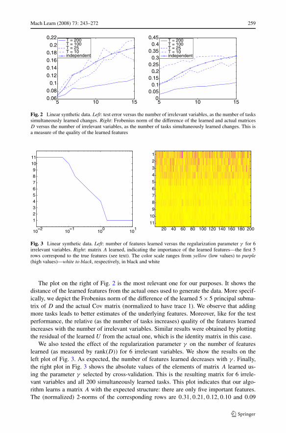
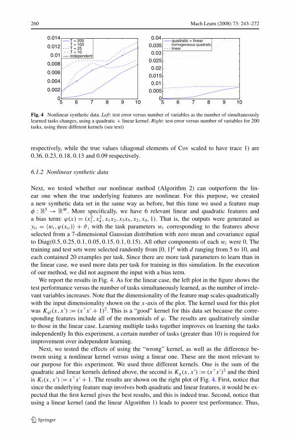
Fig. 2 Linear synthetic data. Left: test error versus the number of irrelevant variables, as the number of taskssimultaneously learned changes. Right: Frobenius norm of the difference of the learned and actual matricesD versus the number of irrelevant variables, as the number of tasks simultaneously learned changes. This isa measure of the quality of the learned features
Fig. 3 Linear synthetic data. Left: number of features learned versus the regularization parameter γ for 6irrelevant variables. Right: matrix A learned, indicating the importance of the learned features—the first 5rows correspond to the true features (see text). The color scale ranges from yellow (low values) to purple(high values)—white to black, respectively, in black and white
The plot on the right of Fig. 2 is the most relevant one for our purposes. It shows thedistance of the learned features from the actual ones used to generate the data. More specif-ically, we depict the Frobenius norm of the difference of the learned 5 × 5 principal subma-trix of D and the actual Cov matrix (normalized to have trace 1). We observe that addingmore tasks leads to better estimates of the underlying features. Moreover, like for the testperformance, the relative (as the number of tasks increases) quality of the features learnedincreases with the number of irrelevant variables. Similar results were obtained by plottingthe residual of the learned U from the actual one, which is the identity matrix in this case.
We also tested the effect of the regularization parameter γ on the number of featureslearned (as measured by rank(D)) for 6 irrelevant variables. We show the results on theleft plot of Fig. 3. As expected, the number of features learned decreases with γ . Finally,the right plot in Fig. 3 shows the absolute values of the elements of matrix A learned us-ing the parameter γ selected by cross-validation. This is the resulting matrix for 6 irrele-vant variables and all 200 simultaneously learned tasks. This plot indicates that our algo-rithm learns a matrix A with the expected structure: there are only five important features.The (normalized) 2-norms of the corresponding rows are 0.31,0.21,0.12,0.10 and 0.09
260 Mach Learn (2008) 73: 243–272
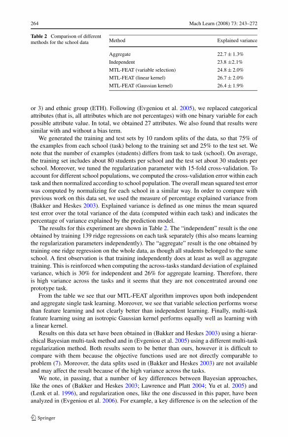
Fig. 4 Nonlinear synthetic data. Left: test error versus number of variables as the number of simultaneouslylearned tasks changes, using a quadratic + linear kernel. Right: test error versus number of variables for 200tasks, using three different kernels (see text)
respectively, while the true values (diagonal elements of Cov scaled to have trace 1) are0.36,0.23,0.18,0.13 and 0.09 respectively.
6.1.2 Nonlinear synthetic data
Next, we tested whether our nonlinear method (Algorithm 2) can outperform the lin-ear one when the true underlying features are nonlinear. For this purpose, we createda new synthetic data set in the same way as before, but this time we used a feature mapφ : R
5 → RM . More specifically, we have 6 relevant linear and quadratic features and
a bias term: ϕ(x) = (x21 , x
24 , x1x2, x3x5, x2, x4,1). That is, the outputs were generated as
yti = 〈wt,ϕ(xti)〉 + ϑ , with the task parameters wt corresponding to the features aboveselected from a 7-dimensional Gaussian distribution with zero mean and covariance equalto Diag(0.5,0.25,0.1,0.05,0.15,0.1,0.15). All other components of each wt were 0. Thetraining and test sets were selected randomly from [0,1]d with d ranging from 5 to 10, andeach contained 20 examples per task. Since there are more task parameters to learn than inthe linear case, we used more data per task for training in this simulation. In the executionof our method, we did not augment the input with a bias term.
We report the results in Fig. 4. As for the linear case, the left plot in the figure shows thetest performance versus the number of tasks simultaneously learned, as the number of irrele-vant variables increases. Note that the dimensionality of the feature map scales quadraticallywith the input dimensionality shown on the x-axis of the plot. The kernel used for this plotwas Kql(x, x ′) := (xx ′ + 1)2. This is a “good” kernel for this data set because the corre-sponding features include all of the monomials of ϕ. The results are qualitatively similarto those in the linear case. Learning multiple tasks together improves on learning the tasksindependently In this experiment, a certain number of tasks (greater than 10) is required forimprovement over independent learning.
Next, we tested the effects of using the “wrong” kernel, as well as the difference be-tween using a nonlinear kernel versus using a linear one. These are the most relevant toour purpose for this experiment. We used three different kernels. One is the sum of thequadratic and linear kernels defined above, the second is Kq(x, x ′) := (xx ′)2 and the thirdis Kl(x, x ′) := xx ′ + 1. The results are shown on the right plot of Fig. 4. First, notice thatsince the underlying feature map involves both quadratic and linear features, it would be ex-pected that the first kernel gives the best results, and this is indeed true. Second, notice thatusing a linear kernel (and the linear Algorithm 1) leads to poorer test performance. Thus,

Mach Learn (2008) 73: 243–272 261
Fig. 5 Matrix A learned in thenonlinear synthetic dataexperiment. The first 7 rowscorrespond to the true features(see text)
our nonlinear Algorithm 2 can exploit the higher approximating power of the most complexkernel in order to obtain better performance.
Finally, Fig. 5 contains the plot of matrix A learned for this experiment using kernelKql , no irrelevant variables and all 200 tasks simultaneously, as we did in Fig. 3 for thelinear case. Similarly to the linear case, our method learns a matrix A with the desiredstructure: only the first 7 rows have large entries. Note that the first 7 rows correspond to themonomials of ϕ, while the remaining 14 rows correspond to the other monomial componentsof the feature map associated with the kernel.
6.2 Conjoint analysis experiment
Next, we tested our algorithms using a real data set from (Lenk et al. 1996) about people’sratings of products.3 The data was taken from a survey of 180 persons who rated the like-lihood of purchasing one of 20 different personal computers. Here the persons correspondto tasks and the computer models to examples. The input is represented by the following13 binary attributes: telephone hot line (TE), amount of memory (RAM), screen size (SC),CPU speed (CPU), hard disk (HD), CD-ROM/multimedia (CD), cache (CA), color (CO),availability (AV), warranty (WA), software (SW), guarantee (GU) and price (PR). We alsoadded an input component accounting for the bias term. The output is an integer rating onthe scale 0–10. As in one of the cases in (Lenk et al. 1996), for this experiment we used thefirst 8 examples per task as the training data and the last 4 examples per task as the test data.We measure the root mean square error of the predicted from the actual ratings for the testdata, averaged across the people.
We show results for the linear Algorithm 1 in Fig. 6. In agreement with the simulationsresults above and past empirical and theoretical evidence (see example in Baxter 2000),the performance of Algorithm 1 improves as the number of tasks increases. It also performsbetter for all 180 tasks with a test error of 1.93 as compared to independent ridge regressionswith a test error of 3.88. Moreover, as shown in Fig. 7, the number of features learneddecreases as the regularization parameter γ increases, as expected.
This data has been used also in (Evgeniou et al. 2006). One of the empirical findingsof (Evgeniou et al. 2006; Lenk et al. 1996), a standard one regarding people’s preferences,is that estimation improves when one also shrinks the individual wt ’s towards a “mean ofthe tasks”, for example the mean of all the wt ’s. Hence, it may be more appropriate for thisdata set to use the regularization term
∑T
t=1 〈(wt − w0),D+(wt − w0)〉 as in (Evgeniou et
3We would like to thank Peter Lenk for kindly sharing this data set with us.

262 Mach Learn (2008) 73: 243–272
Fig. 6 Conjoint experiment withcomputer survey data: averageroot mean square error vs.number of tasks
Fig. 7 Conjoint experiment withcomputer survey data: number offeatures learned (with 180 tasks)versus the regularizationparameter γ
Table 1 Comparison of differentmethods for the computer surveydata. MTL-FEAT is the methoddeveloped here
Method RMSE
Independent 3.88
Hierarchical Bayes (Lenk et al. 1996) 1.90
RR-Het (Evgeniou et al. 2006) 1.79
MTL-FEAT (linear kernel) 1.93
MTL-FEAT (Gaussian kernel) 1.85
MTL-FEAT (variable selection) 2.01
al. 2006) (see above) instead of∑T
t=1 〈wt,D+wt 〉 which we use here. Indeed, test perfor-
mance is better with the former than the latter. The results are summarized in Table 1. Wealso note that the hierarchical Bayes method of (Lenk et al. 1996), similar to that of (Bakkerand Heskes 2003), also shrinks the wt ’s towards a mean across the tasks. Algorithm 1 per-forms similarly to hierarchical Bayes (despite not shrinking towards a mean of the tasks) butworse than the method of (Evgeniou et al. 2006). However, we are mainly interested here inlearning the common across people/tasks features. We discuss this next.
We investigate which features are important to all consumers as well as how these fea-tures weight the 13 computer attributes. We demonstrate the results in the two adjacent plotsof Fig. 8, which were obtained by simultaneously learning all 180 tasks. The plot on the leftshows the absolute values of matrix A of feature coefficients learned for this experiment.This matrix has only a few large rows, that is, only a few important features are learned. In

Mach Learn (2008) 73: 243–272 263
Fig. 8 Conjoint experiment with computer survey data. Left: matrix A learned, indicating the importance offeatures learned for all 180 tasks simultaneously. Right: the most important feature learned, common acrossthe 180 people/tasks simultaneously learned
addition, the coefficients in each of these rows do not vary significantly across tasks, whichmeans that the learned feature representation is shared across the tasks. The plot on the rightshows the weight of each input variable in the most important feature. This feature seemsto weight the technical characteristics of a computer (RAM, CPU and CD-ROM) against itsprice. Note that (as mentioned in the introduction) this is different from selecting the mostimportant variables. In particular, in this case the relative “weights” of the 4 variables usedin this feature (RAM, CPU, CD-ROM and price) are fixed across all tasks/people.
We also tested our multi-task variable selection method, which constrains matrix D in Al-gorithm 1 to be diagonal. This method led to inferior performance. Specifically, for T = 180,multi-task variable selection had test error equal to 2.01, which is worse than the 1.93 er-ror achieved with multi-task feature learning. This supports the argument that “good” fea-tures should combine multiple attributes in this problem. Finally, we tested Algorithm 2with a Gaussian kernel, achieving a slight improvement in performance—see Table 1. Byconsidering radial kernels of the form K(x,x ′) = e−ω‖x−x′‖2
and selecting ω through cross-validation, we obtained a test error of 1.85 for all 180 tasks. However, interpreting the fea-tures learned is more complicated in this case, because of the infinite dimensionality of thefeature map for the Gaussian kernel.
6.3 School data
We have also tested our algorithms on the data from the Inner London Education Authority.4
This data set has been used in previous work on multitask learning, for example in (Bakkerand Heskes 2003; Evgeniou et al. 2005; Goldstein 1991). It consists of examination scoresof 15362 students from 139 secondary schools in London during the years 1985, 1986 and1987. Thus, there are 139 tasks, corresponding to predicting student performance in eachschool. The input consists of the year of the examination (YR), 4 school-specific and 3student-specific attributes. Attributes which are constant in each school in a certain year are:percentage of students eligible for free school meals, percentage of students in VR band one(highest band in a verbal reasoning test), school gender (S.GN.) and school denomination(S.DN.). Student-specific attributes are: gender (GEN), VR band (can take the values 1, 2
4Available at http://www.mlwin.com/intro/datasets.html.
264 Mach Learn (2008) 73: 243–272
Table 2 Comparison of differentmethods for the school data Method Explained variance
Aggregate 22.7 ± 1.3%
Independent 23.8 ±2.1%
MTL-FEAT (variable selection) 24.8 ± 2.0%
MTL-FEAT (linear kernel) 26.7 ± 2.0%
MTL-FEAT (Gaussian kernel) 26.4 ± 1.9%
or 3) and ethnic group (ETH). Following (Evgeniou et al. 2005), we replaced categoricalattributes (that is, all attributes which are not percentages) with one binary variable for eachpossible attribute value. In total, we obtained 27 attributes. We also found that results weresimilar with and without a bias term.
We generated the training and test sets by 10 random splits of the data, so that 75% ofthe examples from each school (task) belong to the training set and 25% to the test set. Wenote that the number of examples (students) differs from task to task (school). On average,the training set includes about 80 students per school and the test set about 30 students perschool. Moreover, we tuned the regularization parameter with 15-fold cross-validation. Toaccount for different school populations, we computed the cross-validation error within eachtask and then normalized according to school population. The overall mean squared test errorwas computed by normalizing for each school in a similar way. In order to compare withprevious work on this data set, we used the measure of percentage explained variance from(Bakker and Heskes 2003). Explained variance is defined as one minus the mean squaredtest error over the total variance of the data (computed within each task) and indicates thepercentage of variance explained by the prediction model.
The results for this experiment are shown in Table 2. The “independent” result is the oneobtained by training 139 ridge regressions on each task separately (this also means learningthe regularization parameters independently). The “aggregate” result is the one obtained bytraining one ridge regression on the whole data, as though all students belonged to the sameschool. A first observation is that training independently does at least as well as aggregatetraining. This is reinforced when computing the across-tasks standard deviation of explainedvariance, which is 30% for independent and 26% for aggregate learning. Therefore, thereis high variance across the tasks and it seems that they are not concentrated around oneprototype task.
From the table we see that our MTL-FEAT algorithm improves upon both independentand aggregate single task learning. Moreover, we see that variable selection performs worsethan feature learning and not clearly better than independent learning. Finally, multi-taskfeature learning using an isotropic Gaussian kernel performs equally well as learning witha linear kernel.
Results on this data set have been obtained in (Bakker and Heskes 2003) using a hierar-chical Bayesian multi-task method and in (Evgeniou et al. 2005) using a different multi-taskregularization method. Both results seem to be better than ours, however it is difficult tocompare with them because the objective functions used are not directly comparable toproblem (7). Moreover, the data splits used in (Bakker and Heskes 2003) are not availableand may affect the result because of the high variance across the tasks.
We note, in passing, that a number of key differences between Bayesian approaches,like the ones of (Bakker and Heskes 2003; Lawrence and Platt 2004; Yu et al. 2005) and(Lenk et al. 1996), and regularization ones, like the one discussed in this paper, have beenanalyzed in (Evgeniou et al. 2006). For example, a key difference is on the selection of the

Mach Learn (2008) 73: 243–272 265
Fig. 9 School data. Left: matrix A learned for the school data set using a linear kernel. For clarity, onlythe 15 most important learned features/rows are shown. Right: The most important feature learned, commonacross all 139 schools/tasks simultaneously learned
regularization parameter γ , which for Bayesian methods is to some extent determined froma prior distribution while in our case it is selected from the data using, for example, cross-validation. We refer the reader to (Evgeniou et al. 2006) for more information on this issueas well as other similarities and differences between the two approaches.
This data set seems well-suited to the approach we have proposed, as one may expectthe learning tasks to be very related without being the same—as also discussed in (Bakkerand Heskes 2003; Evgeniou et al. 2005)—in the sense assumed in this paper. Indeed, onemay expect that academic achievement should be influenced by the same variables acrossschools, if we exclude statistical variation of the student population within each school.This is confirmed in Fig. 9, where the learned coefficients and the most important featureare shown. As expected, the predicted examination score depends very strongly on the stu-dent’s VR band. The other variables are much less significant. Ethnic background (primarilyBritish-born, Carribean and Indian) and gender have the next largest influence. What is moststriking perhaps is that none of the school-specific attributes has any noticeable significance.
Finally, the effects of the number of tasks on the test performance and of the regular-ization parameter γ on the number of features learned are similar to those for the conjointand synthetic data: as the number of tasks increases, test performance improves and as γ
increases sparsity increases. These plots are similar to Figs. 6 and 7 and are not shown forbrevity.
6.4 Dermatology data
Finally, we show a real-data experiment where it seems (as these are real data, we cannotknow for sure whether indeed this is the case) that the tasks are unrelated (at least in the waywe have defined in this paper). In this case, our methods find features which are differentacross the tasks, and do not improve or decrease performance relative to learning each taskindependently.
We used the UCI dermatology data set5 as in (Jebara 2004). The problem is a multi-class one, namely to diagnose one of six dermatological diseases based on 33 clinical andhistopathological attributes (and an additional bias component). As in the aforementioned
5Available at http://www.ics.uci.edu/mlearn/MLSummary.html.

266 Mach Learn (2008) 73: 243–272
Fig. 10 Dermatology data.Feature coefficients matrix A
learned, using a linear kernel
Table 3 Performance of thealgorithms for the dermatologydata
Method Misclassifications
Independent (linear) 16.5 ± 4.0
MTL-FEAT (linear) 16.5 ± 2.6
Independent (Gaussian) 9.8 ± 3.1
MTL-FEAT (Gaussian) 9.5 ± 3.0
paper, we obtained a multi-task problem from the six binary classification tasks. We dividedthe data set into 10 random splits of 200 training and 166 testing points and measured theaverage test error across these splits.
We report the misclassification test error in Table 3. Algorithm 1 gives similar perfor-mance to that obtained in (Jebara 2004) with joint feature selection and linear SVM classi-fiers. However, similar performance is also obtained by training 6 independent classifiers.The test error decreased when we ran Algorithm 2 with a single-parameter Gaussian kernel,but it is again similar to that obtained by training 6 independent classifiers with a Gaussiankernel. Hence one may conjecture that these tasks are weakly related to each other or unre-lated in the way we define in this paper.
To further explore this point, we show the matrix A learned by Algorithm 1 in Fig. 10.This figure indicates that different tasks (diseases) are explained by different features. Theseresults reinforce our hypothesis that these tasks may be independent. They indicate that insuch a case our methods do not “hurt” performance by simultaneously learning all tasks.In other words, in this problem our algorithms did learn a “sparse common representation”but did not—and probably should not—force each feature learned to be equally importantacross the tasks.
7 Discussion
We have presented an algorithm which learns common sparse representations across a poolof related tasks. These representations are assumed to be orthonormal functions in a repro-ducing kernel Hilbert space. Our method is based on a regularization problem with a noveltype of regularizer, which is a mixed (2,1)-norm.
We showed that this problem, which is non-convex, can be reformulated as a convexoptimization problem. This result makes it possible to compute the optimal solutions usinga simple alternating minimization algorithm, whose convergence we have proven. For the

Mach Learn (2008) 73: 243–272 267
case of a high-dimensional feature map, we have developed a variation of the algorithmwhich uses kernel functions. We have also proposed a variation of the first algorithm forsolving the problem of multi-task feature selection with a linear feature map.
We have reported experiments with our method on synthetic and real data. They indicatethat our algorithms learn sparse feature representations common to all the tasks wheneverthis helps improve performance. In this case, the performance obtained is better than thatof training the tasks independently. Moreover, when applying our algorithm on a data setwith weak task interdependence, performance does not deteriorate and the representationlearned reflects the lack of task relatedness. As indicated in one such experiment, one canalso use the estimated matrix A to visualize the task relatedness. Finally, our experimentshave shown that learning orthogonal features improves on just selecting input variables.
To our knowledge, our approach provides the first convex optimization formulationfor multi-task feature learning. Although convex optimization methods have been de-rived for the simpler problem of feature selection (Jebara 2004), prior work on multi-task feature learning has been based on more complex optimization problems which arenot convex (Ando and Zhang 2005; Baxter 2000; Caruana 1997) and, so, these meth-ods are not guaranteed to converge to a global minimum. In particular, in (Baxter 2000;Caruana 1997) different neural networks with one or more hidden layers are trained for eachtask and they all share the same hidden weights. These common hidden layers and weightsact as an internal representation (like the features in our formulation) which is shared by allthe tasks.
Our algorithm also shares some similarities with recent work in (Ando and Zhang 2005)where they alternately update the task parameters and the features. Two main differencesare that their formulation is not convex and that, in our formulation, the number of learnedfeatures is not fixed in advance but it is controlled by a regularization parameter.
As noted in Sect. 4, our work relates to that in (Abernethy et al. 2006; Srebro et al. 2005),which investigate regularization with the trace norm in the context of collaborative filtering.In fact, the sparsity assumption which we have made in our work, starting with the (2,1)-norm, connects to the low rank assumption in that work. Hence, it may be possible thatour alternating algorithm, or some variation of it, could be used to solve the optimizationproblems of (Srebro et al. 2005; Abernethy et al. 2006). Such an algorithm could be usedwith any convex loss function.
Other interesting approaches which may be pursued in the context of multi-task learninginclude multivariate linear models in statistics such as reduced rank regression (Izenman1975), partial least squares (Wold et al. 1984) and canonical correlation analysis (Hotelling1936) (see also Breiman and Friedman 1997). These methods are based on generalizedeigenvalue problems—see, for example, (Borga 1998, Chap. 4) for a nice review. They havealso been extended in an RKHS setting, see, for example, (Bennett and Embrechts 2003;Hardoon et al. 2004) and references therein. Although these methods have proved useful inpractical applications, they require that the same input examples are shared by all the tasks.On the contrary, our approach does not rely on this assumption.
Our work may be extended in different directions. First, it would be interesting to carryout a learning theory analysis of the algorithms presented in this paper. Results in (Capon-netto and De Vito 2006; Maurer 2006) may be useful for this purpose. Another interestingquestion is to study how the solution of our algorithms depends on the regularization para-meter and investigate conditions which ensure that the number of features learned decreaseswith the degree of regularization, as we have experimentally observed in this paper. Resultsin (Micchelli and Pinkus 1994) may be useful for this purpose.
Second, on the algorithmic side, it would be interesting to explore whether our formula-tion can be extended to the more general class of spectral norms in place of the trace norm.
268 Mach Learn (2008) 73: 243–272
A special case of interest is the (2,p)-norm for p ∈ [1,∞). This question is being addressedin (Argyriou et al. 2007b).
Finally, a promising research direction is to explore whether different assumptions aboutthe features (other than the orthogonality one which we have made throughout this paper)can still lead to different convex optimization methods for learning other types of features.More specifically, it would be interesting to study whether non-convex models for learningstructures across the tasks, like those in (Zhang et al. 2006) where ICA type features arelearned, or hierarchical features models like in (Torralba et al. 2004), can be reformulated inour framework.
Acknowledgements We wish to thank Raphael Hauser and Ying Yiming for observations which led toProposition 1, Zoubin Ghahramani, Trevor Hastie, Mark Herbster, Andreas Maurer, Sayan Mukherjee, JohnShawe-Taylor, as well as the anonymous referees for useful comments and Peter Lenk for kindly sharing hisdata set with us. A special thanks to Charles Micchelli for many useful insights.
This work was supported by EPSRC Grants GR/T18707/01 and EP/D071542/1 and by the IST Pro-gramme of the European Community, under the PASCAL Network of Excellence IST-2002-506778.
Appendix 1: Proof of (13)
Proof Consider a matrix C ∈ Sd+. We will compute inf{trace(D−1C) : D ∈ Sd++, trace(D)
≤ 1}. From the Cauchy-Schwarz inequality for the Frobenius norm, we obtain
trace(D−1C) ≥ trace(D−1C) trace(D)
= trace((D− 12 C
12 )(C
12 D− 1
2 )) trace(D12 D
12 )
≥ (trace(D12 (C
12 D− 1
2 )))2 = (traceC12 )2.
The equality is attained if and only if trace(D) = 1 and C12 D− 1
2 = aD12 for some a ∈ R, or
equivalently for D = C12
traceC12
. �
Using similar arguments as above, it can be shown that min{trace(D+C) : D ∈ Sd+,
trace(D) ≤ 1, range(C) ⊆ range(D)} also equals (traceC12 )2.
Appendix 2: Convergence of Algorithm 1
In this appendix, we present the proofs of Theorems 2 and 3. For this purpose, we substi-tute (13) in the definition of Rε obtaining the objective function
Sε(W) := Rε(W,Dε(W))
=T∑
t=1
m∑
i=1
L(yti , 〈wt, xti〉) + γ (trace(WW + εI)12 )2.
Moreover, we define the following function which formalizes the supervised step of thealgorithm,
gε(W) := min{Rε(V ,Dε(W)), : V ∈ Rd×T }.

Mach Learn (2008) 73: 243–272 269
Since Sε(W) = Rε(W,Dε(W)) and Dε(W) minimizes Rε(W, ·), we obtain that
Sε(W(n+1)) ≤ gε(W
(n)) ≤ Sε(W(n)). (23)
We begin by observing that Sε has a unique minimizer. This is a direct consequence ofthe following proposition.
Proposition 3 The function Sε is strictly convex for every ε > 0.
Proof It suffices to show that the function
W �→ (trace(WW + εI)12 )2
is strictly convex. But this is simply a spectral function, that is, a function of the singularvalues of W . By (Lewis 1995, Sect. 3), strict convexity follows directly from strict convexity
of the real function σ �→ (∑
i
√σ 2
i + ε)2. This function is strictly convex because it is thesquare of a positive strictly convex function. �
We note that when ε = 0, the function Sε is regularized by the trace norm squared whichis not a strictly convex function. Thus, in many cases of interest S0 may have multipleminimizers. For instance, this is true if the loss function L is not strictly convex, which isthe case with SVMs.
Next, we show the following continuity property which underlies the convergence ofAlgorithm 1.
Lemma 2 The function gε is continuous for every ε > 0.
Proof We first show that the function Gε : Sd++ → R defined as
Gε(D) := min{Rε(V ,D) : V ∈ Rd×T }
is convex. Indeed, Gε is the minimal value of T separable regularization problems witha common kernel function determined by D. For a proof that the minimal value of a 2-normregularization problem is convex in the kernel, see (Argyriou et al. 2005, Lemma 2). Sincethe domain of this function is open, Gε is also continuous (see Borwein and Lewis 2005,Sect. 4.1).
In addition, the matrix-valued function W �→ (WW + εI)12 is continuous. To see this,
we recall the fact that the matrix-valued function Z ∈ Sd+ �→ Z12 is continuous. Continuity
of the matrix square root is due to the fact that the square root function on the reals, t �→ t12 ,
is operator monotone—see e.g., (Bhatia 1997, Sect. X.1).Combining, we obtain that gε is continuous, as the composition of continuous func-
tions. �
Proof of Theorem 2 By inequality (23) the sequence {Sε(W(n)) : n ∈ N} is nonincreas-
ing and, since L is bounded from below, it is bounded. As a consequence, as n → ∞,Sε(W
(n)) converges to a number, which we denote by Sε . We also deduce that the sequence{trace(W(n)W(n) + εI)
12 : n ∈ N} is bounded and hence so is the sequence {W(n) : n ∈ N}.
Consequently there is a convergent subsequence {W(n�) : � ∈ N}, whose limit we denoteby W .
270 Mach Learn (2008) 73: 243–272
Since Sε(W(n�+1)) ≤ gε(W
(n�)) ≤ Sε(W(n�)), gε(W
(n�)) converges to Sε . Thus, byLemma 2 and the continuity of Sε , gε(W ) = Sε(W ). This implies that W is a minimizerof Rε(·,Dε(W )), because Rε(W ,Dε(W )) = Sε(W ).
Moreover, recall that Dε(W ) is the minimizer of Rε(W , ·) subject to the constraints in(12). Since the regularizer in Rε is smooth, any directional derivative of Rε is the sum ofits directional derivatives with respect to W and D. Hence, (W ,Dε(W )) is the minimizerof Rε .
We have shown that any convergent subsequence of {W(n) : n ∈ N} converges to theminimizer of Rε . Since the sequence {W(n) : n ∈ N} is bounded it follows that it convergesto the minimizer as a whole. �
Proof of Theorem 3 Let {(W�n,Dε�n(W�n)) : n ∈ N} be a limiting subsequence of the min-
imizers of {Rε�: � ∈ N} and let (W , D) be its limit as n → ∞. From the definition of
Sε it is clear that min{Sε(W) : W ∈ Rd×T } is a decreasing function of ε and converges to
S = min{S0(W) : W ∈ Rd×T } as ε → 0. Thus, Sε�n
(W�n) → S . Since Sε(W) is continuousin both ε and W (see proof of Lemma 2), we obtain that S0(W ) = S . �
Appendix 3: Proof of Lemma 3
Lemma 3 Let P,N ∈ Rd×T such that P N = 0. Then ‖P + N‖tr ≥ ‖P ‖tr. The equality is
attained if and only if N = 0.
Proof We use the fact that, for matrices A,B ∈ Sn+, A � B implies that traceA12 ≥ traceB
12 .
This is true because the square root function on the reals, t �→ t12 , is operator monotone—
see (Bhatia 1997, Sect. V.1). We apply this fact to the matrices P P + NN and NN toobtain that
‖P + N‖tr = trace((P + N)(P + N))12
= trace(P P + NN)12 ≥ trace(P P )
12 = ‖P ‖tr.
The equality is attained if and only if the spectra of P P + NN and P P are equal,whence trace(NN) = 0, that is N = 0. �
References
Aaker, D. A., Kumar, V., & Day, G. S. (2004). Marketing research (8th ed.). New York: Wiley.Abernethy, J., Bach, F., Evgeniou, T., & Vert, J.-P. (2006). Low-rank matrix factorization with attributes
(Technical Report 2006/68/TOM/DS). INSEAD, Working paper.Ando, R. K., & Zhang, T. (2005). A framework for learning predictive structures from multiple tasks and
unlabeled data. Journal of Machine Learning Research, 6, 1817–1853.Argyriou, A., Micchelli, C. A., & Pontil, M. (2005). Learning convex combinations of continuously para-
meterized basic kernels. In Lecture notes in artificial intelligence: Vol. 3559. Proceedings of the 18thannual conference on learning theory (COLT) (pp. 338–352). Berlin: Springer.
Argyriou, A., Evgeniou, T., & Pontil, M. (2007a). Multi-task feature learning. In Schölkopf, B. Platt, J. Hoff-man, T. (Eds.), Advances in neural information processing systems (Vol. 19, pp. 41–48). Cambridge:MIT Press.
Argyriou, A., Micchelli, C. A., & Pontil, M. (2007b). Representer theorems for spectral norms. Workingpaper, Dept. of Computer Science, University College London.

Mach Learn (2008) 73: 243–272 271
Aronszajn, N. (1950). Theory of reproducing kernels. Transactions of the American Mathematical Society,686, 337–404.
Bakker, B., & Heskes, T. (2003). Task clustering and gating for Bayesian multi–task learning. Journal ofMachine Learning Research, 4, 83–99.
Baxter, J. (2000). A model for inductive bias learning. Journal of Artificial Intelligence Research, 12, 149–198.
Ben-David, S., & Schuller, R. (2003). Exploiting task relatedness for multiple task learning. In Lecture notesin computer science: Vol. 2777. Proceedings of the 16th annual conference on learning theory (COLT)(pp. 567–580). Berlin: Springer.
Bennett, K. P., & Embrechts, M. J. (2003). An optimization perspective on partial least squares. In J. A. K.Suykens, G. Horvath, S. Basu, C. Micchelli, J. Vandewalle (Eds.), NATO science series III: computer &systems sciences: Vol. 190. Advances in learning theory: methods, models and applications (pp. 227–250). Amsterdam: IOS Press.
Bhatia, R. (1997). Matrix analysis. Springer: Graduate texts in Mathematics.Borga, M. (1998). Learning multidimensional signal processing. PhD thesis, Dept. of Electrical Engineering,
Linköping University, Sweden.Borwein, J. M., & Lewis, A. S. (2005). CMS books in mathematics. Convex analysis and nonlinear optimiza-
tion: theory and examples. Berlin: Springer.Boyd, S. P., & Vandenberghe, L. (2004). Convex optimization. Cambridge: Cambridge University Press.Breiman, L., & Friedman, J. H. (1997). Predicting multivariate responses in multiple linear regression. Jour-
nal of the Royal Statistical Society, Series B, 59(1), 3–54.Caponnetto, A., & De Vito, E. (2006). Optimal rates for the regularized least-squares algorithm. Foundations
of Computational Mathematics, August 2006.Caruana, R. (1997). Multi-task learning. Machine Learning, 28, 41–75.Chapelle, O., & Harchaoui, Z. (2005). A machine learning approach to conjoint analysis. In L. K. Saul,
Y. Weiss, & L. Bottou (Eds.), Advances in neural information processing systems (Vol. 17, pp. 257–264). Cambridge: MIT Press.
Donoho, D. (2004). For most large underdetermined systems of linear equations, the minimal l1-norm near-solution approximates the sparsest near-solution. Preprint, Dept. of Statistics, Stanford University.
Evgeniou, T., Micchelli, C. A., & Pontil, M. (2005). Learning multiple tasks with kernel methods. Journal ofMachine Learning Research, 6, 615–637.
Evgeniou, T., Pontil, M., & Toubia, O. (2006). A convex optimization approach to modeling consumer het-erogeneity in conjoint estimation (Technical Report). INSEAD.
Fazel, M., Hindi, H., & Boyd, S. P. (2001). A rank minimization heuristic with application to minimum ordersystem approximation. In Proceedings of the American control conference (Vol. 6, pp. 4734–4739).
Goldstein, H. (1991). Multilevel modelling of survey data. The Statistician, 40, 235–244.Golub, G. H., & van Loan, C. F. (1996). Matrix computations. Baltimore: Johns Hopkins University Press.Hardoon, D. R., Szedmak, S., & Shawe-Taylor, J. (2004). Canonical correlation analysis: an overview with
application to learning methods. Neural Computation, 16(12), 2639–2664.Hastie, T., Tibshirani, R., & Friedman, J. (2001). Springer series in statistics. The elements of statistical
learning: data mining, inference and prediction. Berlin: Springer.Heisele, B., Serre, T., Pontil, M., Vetter, T., & Poggio, T. (2002). Categorization by learning and combining
object parts. In Advances in neural information processing systems (Vol. 14, pp. 1239–1245). Cam-bridge: MIT Press.
Hotelling, H. (1936). Relations between two sets of variates. Biometrika, 28, 321–377.Izenman, A. J. (1975). Reduced-rank regression for the multivariate linear model. Journal of Multivariate
Analysis, 5, 248–264.Jebara, T. (2004). Multi-task feature and kernel selection for SVMs. In Proceedings of the 21st international
conference on machine learning.Lawrence, N. D., & Platt, J. C. (2004). Learning to learn with the informative vector machine. In R. Greiner
(Ed.), Proceedings of the international conference in machine learning. Helsinki: Omnipress.Lenk, P. J., DeSarbo, W. S., Green, P. E., & Young, M. R. (1996). Hierarchical Bayes conjoint analysis:
recovery of partworth heterogeneity from reduced experimental designs. Marketing Science, 15(2), 173–191.
Lewis, A. S. (1995). The convex analysis of unitarily invariant matrix functions. Journal of Convex Analysis,2(1), 173–183.
Maurer, A. (2006). Bounds for linear multi-task learning. Journal of Machine Learning Research, 7, 117–139.
Micchelli, C. A., & Pinkus, A. (1994). Variational problems arising from balancing several error criteria.Rendiconti di Matematica, Serie VII, 14, 37–86.

272 Mach Learn (2008) 73: 243–272
Micchelli, C. A., & Pontil, M. (2005). On learning vector-valued functions. Neural Computation, 17, 177–204.
Neve, M., De Nicolao, G., & Marchesi, L. (2007). Nonparametric identification of population models viaGaussian processes. Automatica (Journal of IFAC), 43(7), 1134–1144.
Obozinski, G., Taskar, B., & Jordan, M. I. (2006). Multi-task feature selection (Technical report). Deptartmentof Statistics, UC Berkeley, June 2006.
Poggio, T., & Girosi, F. (1998). A sparse representation for function approximation. Neural Computation, 10,1445–1454.
Serre, T., Kouh, M., Cadieu, C., Knoblich, U., Kreiman, G., & Poggio, T. (2005). Theory of object recogni-tion: computations and circuits in the feedforward path of the ventral stream in primate visual cortex(AI Memo 2005-036). Massachusetts Institute of Technology.
Srebro, N., Rennie, J. D. M., & Jaakkola, T. S. (2005). Maximum-margin matrix factorization. In Advancesin neural information processing systems (Vol. 17, pp. 1329–1336). Cambridge: MIT Press.
Torralba, A., Murphy, K. P., & Freeman, W. T. (2004). Sharing features: efficient boosting procedures formulticlass object detection. In Proceedings of the IEEE conference on computer vision and patternrecognition (CVPR) (Vol. 2, pp. 762–769).
Wahba, G. (1990). Series in applied mathematics: Vol. 59. Splines models for observational data. Philadel-phia: SIAM.
Wold, S., Ruhe, A., Wold, H., & Dunn III, W. J. (1984). The collinearity problem in linear regression. Thepartial least squares (PLS) approach to generalized inverses. SIAM Journal of Scientific Computing, 3,735–743.
Xue, Y., Liao, X., Carin, L., & Krishnapuram, B. (2007). Multi-task learning for classification with Dirichletprocess priors. Journal of Machine Learning Research, 8, 35–63.
Yu, K., Tresp, V., & Schwaighofer, A. (2005). Learning Gaussian processes from multiple tasks. In Proceed-ings of the 22nd international conference on machine learning.
Zhang, J., Ghahramani, Z., & Yang, Y. (2006). Learning multiple related tasks using latent independentcomponent analysis. In Advances in neural information processing systems (Vol. 18, pp. 1585–1592).Cambridge: MIT Press.