convexity estimates for mean curvature flow and ...js/math646/huisken-sinestrari2.pdf · convexity...
TRANSCRIPT
Acta Math., 183 (1999), 45-70 (~) 1999 by Institut Mittag-Leffler. All rights reserved
C o n v e x i t y e s t i m a t e s for m e a n curvature flow and s ingular i t i e s of m e a n c o n v e x surfaces
GERHARD HUISKEN
Universitiit Ti~bingen Tiibingen, Germany
by
and CARLO SINESTRARI
Universitd di Roma "Tot Vergata" Rome, Italy
1. I n t r o d u c t i o n
Let F0: 2~4-~R ~+1 be a smooth immersion of a closed n-dimensional hypersurface of
nonnegative mean curvature in Euclidean space, n~>2. The evolution of A~o=Fo(J~4) by
mean curvature flow is the one-parameter family of smooth immersions F: J~4 • [0, T[-+
R n+l satisfying
OF ~(p,t)=-H(p,t)~(p,t), pEArl, t>~O, (1.1)
F(. ,0)=Fo, (1.2)
where H(p, t) and ~(p, t) are the mean curvature and the outer normal respectively at the
point F(p, t) of the surface J~4t=F(., t)(J~4). The signs are chosen such that - H v = _ ~
is the mean curvature vector and the mean curvature of a convex surface is positive.
For closed surfaces the solution of (1.1)-(1.2) exists on a finite maximal time interval
[0, T[, 0 < T < c ~ , and the curvature of the surfaces becomes unbounded for t--+T. It is
important to obtain a detailed description of the singular behaviour for t-*T, a future
goal being the topologically controlled extension of the flow past singularities.
In the present paper we use the assumption of nonnegative mean curvature to derive
new a priori estimates from below for all other elementary symmetric functions of the
principal curvatures, strong enough to conclude that any rescaled limit of a singularity
is (weakly) convex.
Let X= (A1, ..., A,) be the principal curvatures of the evolving hypersurfaces .~4t, and
let
s~(,~) = ~ ~ , , ~ , ~ ... ~,~ l~ i l< i2<. . .< ik~n
46 G. H U I S K E N AND C. S I N E S T R A R I
be the elementary symmetric functions with S I = H . Then our main result is
THEOREM 1.1. Suppose that F0:J~4---~R n+l is a smooth closed hypersurface im-
mersion with nonnegative mean curvature. For each k, 2 ~ k ~ n , and any ~?>0 there is
a constant C~,k depending only on n, k, 77 and the initial data, such that everywhere on
A/[ x [0, T[ we have the estimate
Sk >~ -~?H k - C,7,k. (1.3)
The arbitrariness of y breaks the scaling invariance in inequality (1.3) and implies
that near a singularity, where S I = H becomes unbounded, each Sk becomes nonnegative
after rescaling:
COROLLARY 1.2. Let A/it be a mean convex solution of mean curvature flow on
the maximal time interval [0,T[ as in Theorem 1.1. Then any smooth rescaling of the
singularity for t--~T is convex.
For a discussion of previous results on the blowup behaviour of mean curvature flow
see [12], where we proved a lower bound as in (1.3) for the scalar curvature of A4t. We
note that the present result applies to type-II singularities which up to now were under-
stood only in the one-dimensional Case. We give a classification of type-II singularities
in the mean convex case in Theorem 4.1, complementary to the known classification of
type-I singularities in [10], [11].
In view of the results in [14] and [9] respectively, Theorem 1.1 and Corollary 1.2
also hold for star-shaped surfaces in R n+l and for mean convex surfaces in smooth
Riemannian manifolds, see Remarks 3.8 and 3.9.
The proof of Theorem 1.1 proceeds by induction on the degree k of the elementary
symmetric polynomial Sk. Assuming that the desired inequalities in (1.3) hold up to some
k>~2, we perturb the second fundamental form A={h~j} by adding a small multiple of
the metric g = {g~j }, setting
bij := h~j +~Hg~j + Dgij (1.4)
for small c>0 and positive D. In view of the induction hypothesis (1.3) we manage to
choose D=D~ in such a way that the elementary symmetric function Sk of the eigenvalues
of {b~j} is strictly positive, allowing us to work with the quotient (2k+l=Sk+l/Sk as a
test function. The algebraic properties of Sk, Sk and Qk+l,Q)k+l established in w in
particular the concavity of Qk+l on the set where Sk >0, turn out to be crucial for the
proof of the a priori estimates in w
CONVEXITY ESTIMATES FOR MEAN CURVATURE FLOW 47
2. Symmetric p o l y n o m i a l s
As we said in the introduction, in this paper we are concerned with symmetric functions
of the principal curvatures on a manifold. We begin by recalling the definition and some
basic properties of the elementary symmetric polynomials. In the following n>~2 is a
fixed integer.
Definition 2.1. For any k = l , 2, ..., n we set
sk(P) : Z p,lu,~ ...p~k, v u = (p~, ..., p , ) eR". (2.1) l <~ il < i2<...<ik <~ n
We also set s 0 - 1 and s k - 0 for k>n. In addition, we define
r k : { p e R " : ~l(p) > 0, ~:(p) > 0, ..., sk(u) > 0}. (2.2)
Clearly the sets Fk are open cones and satisfy Fk+ICFk for any k = l , . . . , n - 1 . In
the sequel (Theorem 2.5 and Proposition 2.6) we will also see that these cones are convex
and that Fn coincides with the positive cone.
Let us denote by Sk;i(p) the sum of the terms of sk(p) not containing the factor Pi.
Then the following identities hold.
PROPOSITION 2.2. We have, for any k=0 , . . . , n , i=1 , ...,n and p c R n,
Osk+l (p) = sk;i(p), (2.3) Op~
Sk+I(P) = sk+l;i(p) +pisk;i(p), (2.4)
~ s~;~(p) = (n- k)s~(p), (2.5) i=1
pisk;,(p) : (k+l)sk+l(p), (2.6) i=1
n
E p28k;i(P) : S l ( P ) S k + l ( P ) - (kJ-2)Sk+2(P)" (2 .7)
i : 1
Proof. The properties (2.3) and (2.4) follow from the definitions, while (2.6) is a
consequence of (2.3) and Euler's theorem on homogeneous functions. Taking sums over
i in (2.4) and applying (2.6) we obtain (2.5). By (2.4) we also obtain, for any p e r u,
sk+~(p)- sk+2;i(p) = p~sk+l;i(p) = P,~k+I(P)--P~sk;,(P).
48 G. HUISKEN AND C. SINESTRARI
Taking sums over i and using (2.5) we find
n
i=1
which implies the identity (2.7). []
A less immediate property of these polynomials is the following inequality (for the
proof see e.g. [7, pp. 104-105]).
THEOREM 2.3. For any kE{1 , . . . , n -1} and # c R '~ we have
(n--k + l )(k + l)sk-a(#)sk+a(#) <<. k(n-k)s2k(#). (2.8)
The above result is known as Newton's inequality. We observe that it implies the
weaker inequality
Sk-l(#)Sk+l(#) <<. S2(U). (2.9)
The following property of the polynomials sk;i is a consequence of Newton's inequality.
LEMMA 2.4. Let # 6 F k be given for some k6{1, . . . ,n}. Then we have Sh;i(#)>0
for any h e { 0 , . . . , k - 1 } and i e{1 , . . . ,n} .
Proof. We proceed by induction on h. The case h = 0 is trivial. Consider now an
arbitrary hE{l , ..., k - l } . By the assumption that #CFk and by (2.4) we have, for any
i=1, ..., n,
U~sh;,(U)+sh+~;~(#) = Sh+l (U) > 0, msh-l#(~)+sh;~(U) = Sh(U) > 0.
By the induction hypothesis we have Sh-1;i(#)>0. Let us argue by contradiction and
suppose that 8h;i(U) ~<~0. Then we have UiSh--1;i(#) =Sh (#)-- Sh;i(U) > 0 , which implies
# i>0. Therefore
~h+l;~(u) > -u~sh;,(~)/> 0, ~,sh-1;i(~) > -sh;~(~)/> 0.
We deduce that Sh+l;~(#)Sh_l;i(#)>s2;i(#). On the other hand, formula (2.9) evalu-
ated for # , = 0 and k = h yields the opposite inequality. The contradiction proves that
sh;~(#)>0. []
Let us now define, for k=2, ..., n and #EFk-1,
sk(#) (2.10) q~(u) = ~-1(#)"
Similarly we set, for i=1, ...,n, qk,i(#)=Sk,i(#)/Sk_l,i(#). Observe that, if #EFk, then
q~,~ (#) is well defined, by virtue of the previous lemma. The functions qk are homogeneous
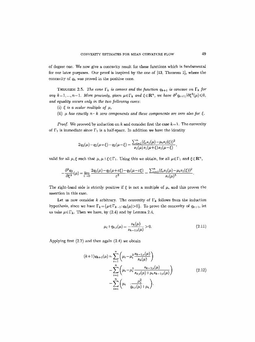
C O N V E X I T Y E S T I M A T E S F O R MEAN CURVATURE F L O W 49
of degree one. We now give a concavity result for these functions which is fundamental
for our later purposes. Our proof is inspired by the one of [13, Theorem 1], where the
concavity of qk was proved in the positive cone.
THEOREM 2.5. The cone Fk is convex and the function qk+l is concave on Fk for
any k = l , . . . , n - 1 . More precisely, given ItEFk and ~ c R n, we have O2qk+l/O~2(it)<~O,
and equality occurs only in the two following cases:
(i) ~ is a scalar multiple of It,
(ii) It has exactly n - k zero components and these components are zero also for ~.
Proof. We proceed by induction on k and consider first the case k = 1. The convexity
of F1 is immediate since F1 is a half-space. In addition we have the identity
2q2(it)-q2(#+~)-q2(it-~)= ~in--l(~isz(It)-Itisl(~))2 Sl(U)sl(it+0sl(it-~)
valid for all It,~ such that It,/t-4-~CI~l. Using this we obtain, for all ItEF1 and ~ c R n,
02q2 2q2( i t ) -q2(#+e~) -q2( i t - e~) ~ 2 E l - - 1 (~i 8 1 ( i t ) - - It i s l (~)) O~ 2 (it) = lim = - ~-+0 e 2 S l ( i t ) 3
The right-hand side is strictly positive if ~ is not a multiple of It, and this proves the
assertion in this case.
Let us now consider k arbitrary. The convexity of Fk follows from the induction
hypothesis, since we have Fk={ i tEFk- l :qk ( i t )>0} . To prove the concavity of qk+l, let
us take #CFk. Then we have, by (2.4) and by Lemma 2.4,
Sk(#) >0. (2.11)
Applying first (2.7) and then again (2.4) we obtain
(k+l)qk+l(#)=i~=l ~#'--#i S--~- ~
, = ,
i=1 qk;i ( ~ + # i "
(2.12)
50 G. H U I S K E N A N D C. S I N E S T R A R I
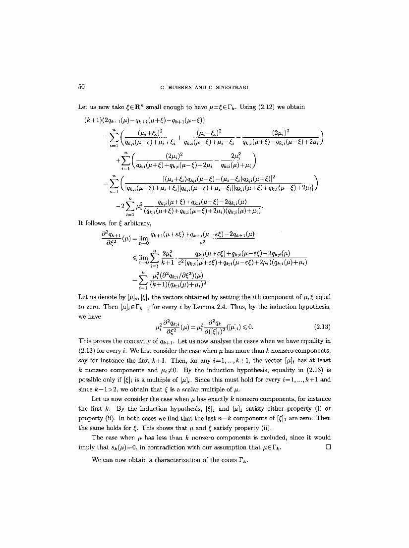
Let us now take ~ E R n small enough to have # • Using (2.12) we obtain
(k+ 1)(2qk+l(#)--qk+l(#+~)--qk+l(#--~))
(
n
i=1 \qk;i(U+~)+qk;i(p--~)+2#i qk;i~7+IZi ]
[(#i+~i)qk;i(#--~)--(#i--~i)qk;~(#+~)] 2 = ~ ([qk;,(#+~)+#~+~,][qk;i(#--~)+#i--~i][qk#(#+~)+qk.i(#--~)+2#i])
i = 1
n qk;i(#+~)+qk;i(#--~)--2qk;i(#) --2 E #2 (qk;i(#+~)+qk',(#--~)+ 2#~)(qk;,(#)+ #,) "
i = l
It follows, for ~ arbitrary,
02qk+l z , qk+l(#+e~)+qk+l(#--e~)--2qk+l(#) ~-~ (#) = lim
r E 2
n
~< lim ~ 2 # ~ 2 qk;i(#+e~)+qk;i(#--e~)--2qk;i(lZ) ~--*0"---' k + l e2(qk;,(#+e~)+qk;,(#--e~)+2#i)(qk#(#)+#~)
i = 1
2 2 2 _= #i(O qk;i/O~ )(#) i=x (k+l)(qk;i(#)+#i)2"
Let us denote by [#]~, [~]~ the vectors obtained by setting the i th component of #, ~ equal
to zero. Then [#]~EFk-1 for every i by Lemma 2.4. Thus, by the induction hypothesis,
we have 02qk;i 2 02qk O U - ( U ) = , , ([U],) < 0. (2.13)
This proves the concavity of qk+l. Let us now analyse the cases when we have equality in
(2.13) for every i. We first consider the ease when # has more than k nonzero components,
say for instance the first k + l . Then, for any i = 1 , . . . , k + 1 , the vector [#]i has at least
k nonzero components and # i r By the induction hypothesis, equality in (2.13) is
possible only if [~]~ is a multiple of [#]~. Since this must hold for every i=1 , ..., k + l and
since k + 1 > 2 , we obtain that ~ is a scalar multiple of #.
Let us now consider the case when # has exactly k nonzero components, for instance
the first k. By the induction hypothesis, [~]1 and [#]1 satisfy either property (i) or
property (ii). In both eases we find that the last n - k components of [~]a are zero. Then
the same holds for ~. This shows that # and ~ satisfy property (ii).
The case when # has less than k nonzero components is excluded, since it would
imply that sk(#)=0, in contradiction with our assumption that #G Fk. []
We can now obtain a characterization of the cones Fk.
CONVEXITy ESTIMATES FOR MEAN CURVATURE FLOW 51
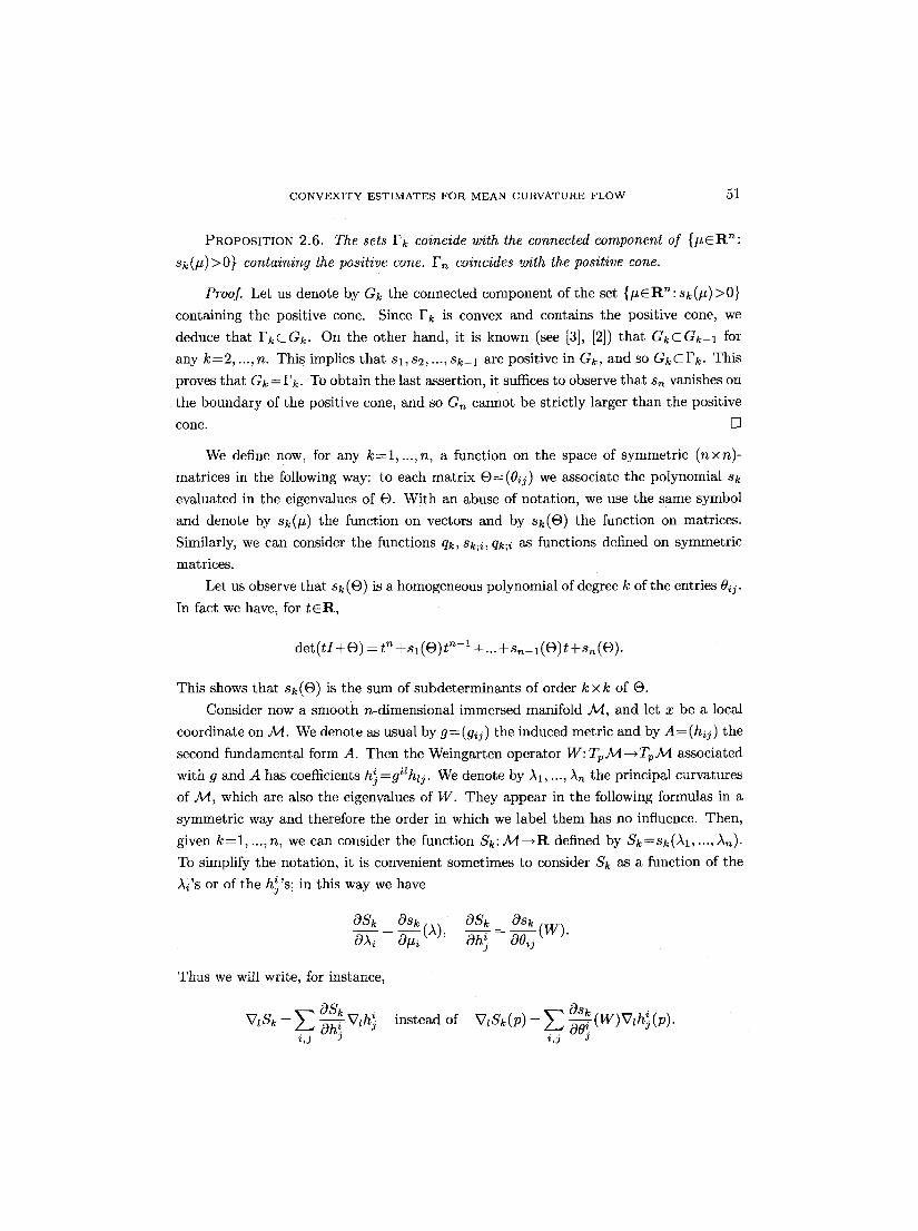
PROPOSITION 2.6. The sets Fk coincide with the connected component of { / t C R n :
Sk(#)>0} containing the positive cone. F~ coincides with the positive cone.
Proof. Let us denote by Gk the connected component of the set { # c R ~ : s k ( # ) > 0 }
containing the positive cone. Since Fk is convex and contains the positive cone, we
deduce that FkCGk. On the other hand, it is known (see [3], [2]) tha t GkCGk-1 for
any k=2 , ...,n. This implies tha t s l , s2, ..., Sk-1 are positive in Gk, and so GkCFk. This
proves tha t Gk = Fk. To obtain the last assertion, it suffices to observe tha t an vanishes on
the boundary of the positive cone, and so G~ cannot be strictly larger than the positive
cone. []
We define now, for any k : l , . . . , n , a function on the space of symmetr ic (n• matrices in the following way: to each matr ix O~(~ i j ) we associate the polynomial sk evaluated in the eigenvalues of 0 . With an abuse of notation, we use the same symbol
and denote by sk(#) the function on vectors and by sk(O) the function on matrices.
Similarly, we can consider the functions qk, sk;i, qk;i as functions defined on symmetric
matrices.
Let us observe that sk(O) is a homogeneous polynomial of degree k of the entries 0ij.
In fact we have, for t E R ,
d e t ( t I + O ) =tn +Sl(O)t~--l +... +Sn_l(O)t +Sn(O).
This shows that Sk(O) is the sum of subdeterminants of order k • of O.
Consider now a smooth n-dimensional immersed manifold A/I, and let x be a local
coordinate on A/[. We denote as usual by g=(gij) the induced metric and by A=(hij) the
second fundamental form A. Then the Weingarten operator W: Tp.M---*TpAJ associated
with g and A has coefficients h} =gilh~j. We denote by As, ...,/~n the principal curvatures
of A/l, which are also the eigenvalues of W. They appear in the following formulas in a
symmetric way and therefore the order in which we label them has no influence. Then,
given k=l, ...,n, we can consider the function Sk: A4--~R defined by Sk=sk()~l, ..., )~). To simplify the notation, it is convenient sometimes to consider Sk as a function of the
A~'s or of the i, hj s; in this way we have
OSk Osk OSk Osk T
Thus we will write, for instance,
OSk i ViSk = ~ . ~ V l h j instead of ~,j 3
52 G. HUISKEN AND C. SINESTRAFtI
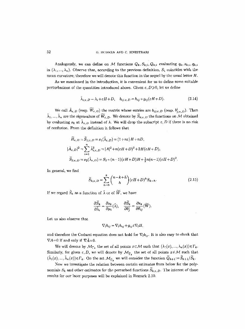
Analogously, we can define on Ad functions Qk, Sk;i, Qk;i evaluating qk, Sk;i, qk;i in (A1, ..., A~). Observe that, according to the previous definition, $1 coincides with the
mean curvature; therefore we will denote this function in the sequel by the usual letter H.
As we mentioned in the introduction, it is convenient for us to define some suitable
perturbations of the quantities introduced above. Given e, D ) 0 , let us define
~i;e,D = )~i+eH+D, bij;s,D = h i j+gi j (eH+D). (2.14)
We call -4~,D (resp. WE,D) the matrix whose entries are bij;e,D (resp. i bj;~,D). Then
~1, ..., ~n are the eigenvalues of W~,D. We denote by Sk;~,D the functions on A4 obtained
by evaluating sk at ~e,D instead of )~. We will drop the subscript e, D if there is no risk
of confusion. From the definition it follows that
ITI~,D = S1;e,o = sl(Ae,z)) = (l +ne )H +nD,
[2~e,D[2 = ~ ~2i;E,D = [A[2+n(sH+D)2+2H(eH+D) , i=1
S2;e,D : 82(~e,D) = S2-~(n-- 1 ) ( r 2.
In general, we find k
S k ; e , D = E ( n - - k + h ) ( e H + D ) h S k _ h �9 h=0
If we regard Sk as a function of A or of W, we have
oh} = ( W )
Let us also observe that
Vzbij = V~hij +gij sVtH,
(2.15)
and therefore the Codazzi equation does not hold for Vzb~j. It is also easy to check that
VA=O if and only if VA=0.
We will denote by Adrk the set of all points xCAd such that (~l(x), ..., ~ ,~(x))erk.
Similarly, for given ~, D, we will denote by 2M~k the set of all points xE3/t such that
( i l (Z), ..., in (X))e Fk. On the set Ad~k we will consider the function Q)k+l :--Sk+l/Sk.
Now we investigate the relation between certain estimates from below for the poly-
nomials Sk and other estimates for the perturbed functions Sk;~,D. The interest of these
results for our later purposes will be explained in Remark 2.10.
C O N V E X I T Y E S T I M A T E S F O R M E A N C U R V A T U R E F L O W 53
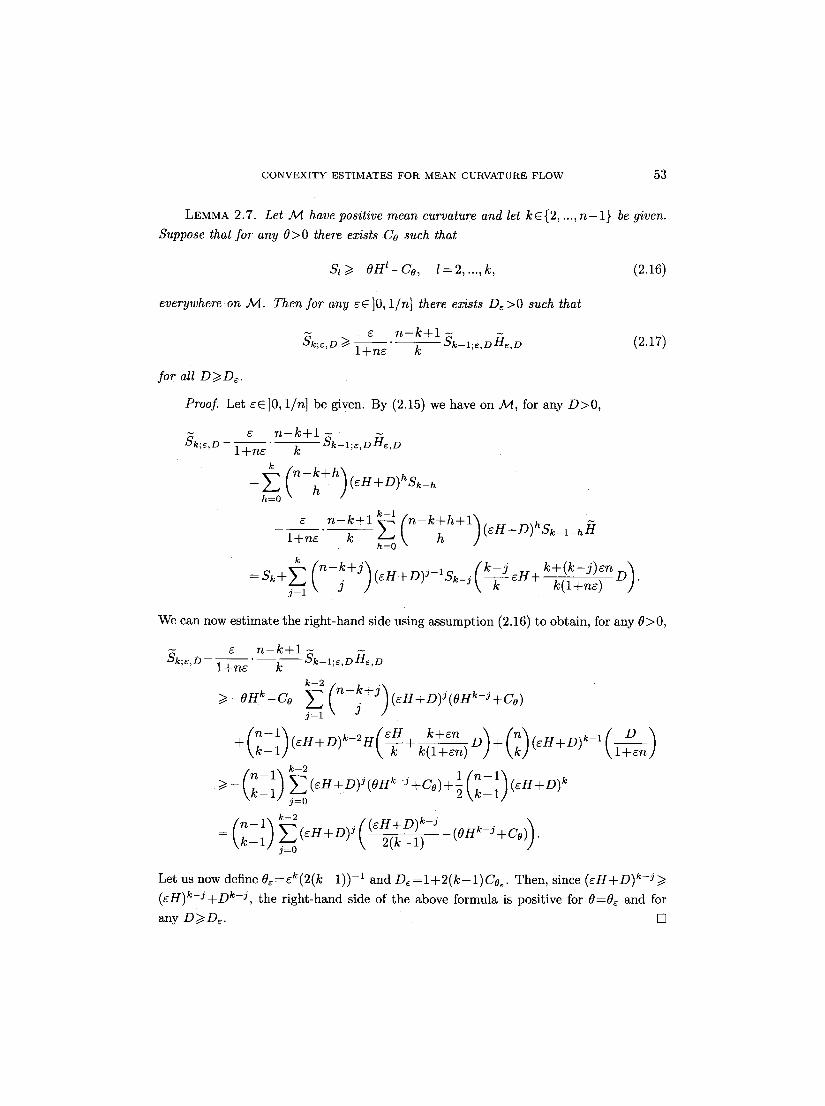
LEMMA 2.7. Let A4 have positive mean curvature and let kE{2, ..., n - l } be given. Suppose that for any 0>0 there exists Co such that
Sz >>. - O H l - C o , 1 = 2, ..., k, (2.16)
everywhere on M. Then for any ee l0 , 1/n] there exists D~>0 such that
r n - k + l ~ Sk;r >~ l + n ~ Sk-1;e,DH~,D (2.17) k
for all D>>.D~.
Proof. Let eE ]0, 1/n] be given. By (2.15) we have on A4, for any D > 0 ,
1 - - t e n - ~ t i - - l + n e k Sk-1;e'DHe'D
k
h = 0
- l+nEe " n - k - t - l ~ ( n - k h h + l ) ( e H + D ) h s k - l - h ~ I - - k h = 0
= S k W ~ - ~ ( n - ; W J ) ( ~ H + D ) J - I s k _ j ( ~ s H 4 kW(k-J )SnD)" j=l " k(l +ne)
We can now estimate the right-hand side using assumption (2.16) to obtain, for any 0>0,
n - k + l S~_l.e D~ie D l +ne k ' ' '
k--2
j = l
+ ( n k - ~ ) ( e H + D ) k _ 2 H ( ~ + k+en D~ D k ( l + e n ) ]+(nk)(eH+D)k-l(1--+~en)
Let us now define 0~ = e k ( 2 ( k - 1)) -1 and De = 1 + 2 ( k - 1) CoG. Then, since (ell+D) k-j >~ (eH)k-J+D k-j, the right-hand side of the above formula is positive for O=0e and for
any D >~ D~. []
54 G. HUISKEN AND C. SINESTRARI
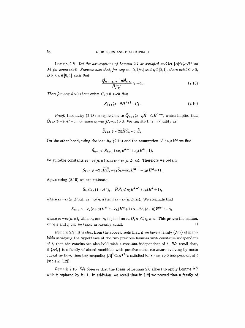
LEMMA 2.8. Let the assumptions of Lemma 2.7 be satisfied and let [A[2<~aH 2 on
M for some a > 0 . Suppose also that, for any r 1/n] and ~/E]0, 1], there exist C>0 ,
D>~0, aE ]0, 1] such that O k + l ; r
- 1 - . ~> - C . (2.18) H~,D
Then for any 0>0 there exists Co>O such that
Sk+l ~ - O H TM - C o . (2.19)
Proof. Inequality (2.18) is equivalent to 0k+ l >/--'11 ~I -C~II -a , which implies that
Qk+l ~ - 2 7 H - C l for some Cl=Cl(C, 7, a )>0 . We rewrite this inequality as
On the other hand, using the identity (2.15) and the assumption IAI2<~aH 2 we find
Sk+l <<. Sk+l +~e2H k+l +c3(H k + 1),
for suitable constants c2=c2(n, a) and c3=c3(n, D, a). Therefore we obtain
Sk+l ~ - 2 7 ~ I S k - Cl S k -- CC2 g k + l -- e3 (H k + 1).
Again using (2.15) we can estimate
Sk <~ c4(l+Hk), f:ISk <~ C5 Hk+l +c6(Hk+l),
where c4 =ca(n, D, a), c5=c5(n, a) and c6 =c6(n, D, a). We conclude that
Sk+l > --C7 (~+7) Hk+l -- c8 (H k + 1) > -2c7 (~+ 7) Hk+l - c9,
where c7=c7(n, a), while c8 and c9 depend on n, D, a, C, 7, a, ~. This proves the lemma,
since ~ and 7 can be taken arbitrarily small. []
Remark 2.9. It is clear from the above proofs that, if we have a family {A/It } of mani-
folds satisfying the hypotheses of the two previous lemmas with constants independent
of t, then the conclusions also hold with a constant independent of t. We recall that ,
if {A/It} is a family of closed manifolds with positive mean curvature evolving by mean
curvature flow, then the inequality ]A] 2 ~ a H 2 is satisfied for some a >0 independent of t
(see e.g. [12]).
Remark 2.10. We observe that the thesis of Lemma 2.8 allows to apply Lemma 2.7
with k replaced by k + l . In addition, we recall that in [12] we proved that a family of
CONVEXITY ESTIMATES FOR MEAN CURVATURE FLOW 55
hypersurfaces evolving by mean curvature flow fulfils property (2.16) for k=2. There-
fore, an iterative application of the two previous lemmas yields our main Theorem 1.1,
provided we are able to prove at each step that estimate (2.18) holds. This will be our
aim in w to this purpose we need some properties of the functions Sk which will be
proved in the remainder of this section.
Following [1, Lemmas 2.22 and 7.12] we now derive some estimates exploiting the
concavity of qk+l. First of all, we derive a suitable expression for the second derivatives
of qk with respect to the matrix entries 0ij in terms of the derivatives of qk with respect
to the eigenvalues #i- Given i,pC {1, ..., n}, with i#p, let us denote by ~ipCR n the vector
whose i th component is 1, the p th component is - 1 , and all other components are 0.
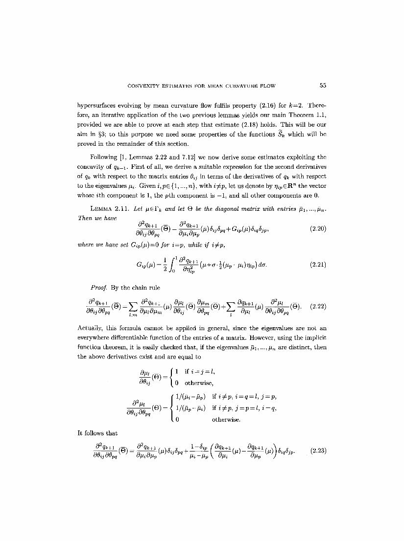
LEIvlMA 2.11. Let [~EPk and let ~) be the diagonal matrix with entries #l,...,ftn. Then we have
02qk+l (~)] 02qk+' (#)SijSpq+Gip(f-t)SiqSjp, (2.20)
where we have set Gip(#)=O for i=p, while if i#p,
1 L 1 02qk+l (p.A-6" l(~tp--~ti)?]ip) da. (2.21) =
Proof. By the chain rule
02qk+l 02qk+l /_, O~l ,~, Ottm .~). ~ Oqk+l ,_, 02l-tl OOijOOpq(~))=E O~--~mt~t)-~ij~w)]-~pq c ) @ L o~-~l t~t] ooijOOp--q (~))" ( 2 . 2 2 )
l,m
Actually, this formula cannot be applied in general, since the eigenvalues are not an
everywhere differentiable function of the entries of a matrix. However, using the implicit
function theorem, it is easily checked that , if the eigenvalues Pl, ..., #n are distinct, then
the above derivatives exist and are equal to
0#L r l i f i=j=l , O0ij (~)) = t 0 otherwise,
o2.z (~)~ { ll(p~-pp) oo pq" "=
0
if i # p , i = q = l , j = p ,
if iT~p, j = p = l , i=q,
otherwise.
It follows that
02qk+l OO i j (~Opq ( ~) )
02qk+l (#)SijSpq+ 1-5ip ( Oqk+l - Oqk+l (r,3~5~ 5 - - _ _ , , , ) ,,,. Otti Ottp tti - t~p \
(2.23)
56 G. H U I S K E N A N D C. S I N E S T R A R I
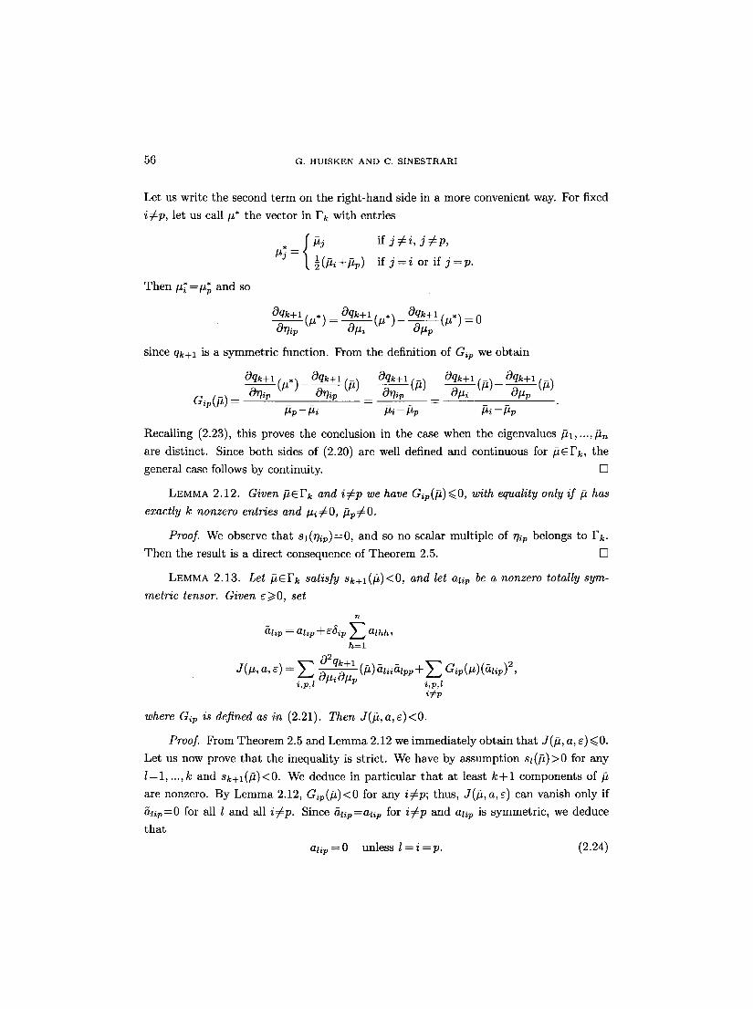
Let us write the second term on the right-hand side in a more convenient way. For fixed
i#p, let us call #* the vector in Fk with entries
�9 {/2j i f j # i , j C p ,
#J = �89 i f j = i or i f j = p .
Then *- * #~ - # p and so
Oqk+l Oqk+l (# . )_ = = o
since qk+l is a symmetric function. From the definition of G~p we obtain
Oqk+l Oqk+l ,_x Oqk+l Oqk+l, ~.~ Oqk+_____! (#) (p) _ ~ L#) a i p @ = - 0 ip _
/2p -/2i /2i -/2p #i - #p
Recalling (2.23), this proves the conclusion in the case when the eigenvalues /21, ...,/2,~
are distinct. Since both sides of (2.20) are well defined and continuous for /2eFk, the
general case follows by continuity. []
LEMMA 2.12. Given/2EFk and i~p we have Gip(/2)<<.O, with equality only if/2 has
exactly k nonzero entries and Pi ~ O, /2p r O.
Proof. We observe that sl(~?ip)=O, and so no scalar multiple of 7/ip belongs to Fk.
Then the result is a direct consequence of Theorem 2.5. []
LEMMA 2.13. Let /2EFk satisfy sk+l(/2)<0, and let alip be a nonzero totally sym-
metric tensor. Given c>~O, set
n
alip z alip ~-Cf~ip E alhh ' h~l
g(/2, a ,e) = ~ ' qk+l - ~ - Gip(#)(Slip)2, ~ (#)az,,azpp+ E i,p,l i,p,l
i#p
where G~p is defined as in (2.21). Then J(/2, a ,E)<0.
Proof. From Theorem 2.5 and Lemma 2.12 we immediately obtain that J(/2, a, E) ~<0.
Let us now prove that the inequality is strict. We have by assumption sz(/2)>0 for any
l=1, . . . , k and sk+l(/2)<0. We deduce in particular tha t at least k + l components of/2
are nonzero. By Lemma 2.12, Gip(/2)<O for any i#p; thus, J(/2, a, E) can vanish only if
~av=0 for all l and all i#p. Since 5av=aap for i #p and aliv is symmetric, we deduce
tha t
Gap = 0 unless l = i = p. (2.24)
C O N V E X I T Y E S T I M A T E S F O R M E A N C U R V A T U R E F L O W 57
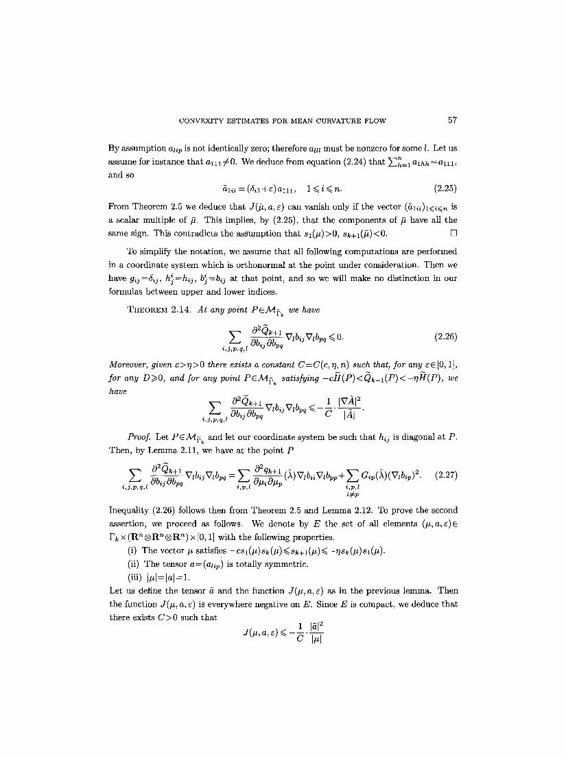
By assumption Clip is not identically zero; therefore am must be nonzero for some I. Let us
assume for instance that al l i ~ 0. We deduce from equation (2.24) that ~h= 1 alhh = al 11, and so
Ctlii =(5/lq-~)alll, 1 <~i<<.n. (2.25)
From Theorem 2.5 we deduce that J(#, a, ~) can vanish only if the vector (51ii)l~<i~<n is
a scalar multiple of/2. This implies, by (2.25), that the components of p have all the
same sign. This contradicts the assumption that s1(/2)>0, Sk+l(#)<0. []
To simplify the notation, we assume that all following computations are performed
in a coordinate system which is orthonormal at the point under consideration. Then we
have gij=Sij, h}=hij, b}=bij at that point, and so we will make no distinction in our
formulas between upper and lower indices.
THEOREM 2.14. At any point PE.a/Ipk we have
020.k+1 v,b jv, bpq .< o. (2.26) i , j ,p,q,l
Moreover, given c>r l>0 there exists a constant C=C(c, rh n) such that, for any ~E[0, 1],
for any D>>.O, and for any point PcA4pk satisfying --c~I(P)<O.k+l(P)<--rl~I(P), we have
02Qk+l 1 IVAI 2 E ~ q V t b i j V l b p q <~ C I]t[
i , j ,p,q,l
Proof. Let PEA//~k and let our coordinate system be such that hij is diagonal at P.
Then, by Lemma 2.11, we have at the point P
E ~OaQk+l VtijVZvpqb ~ = E O#iO#pO2qk+l (A)VzbiiVzbpp+ E Gip(A)(Vlbip) 2. (2.27) i , j ,p,q,l i,p,l i,p,l
i~p
Inequality (2.26) follows then from Theorem 2.5 and Lemma 2.12. To prove the second
assertion, we proceed as follows. We denote by E the set of all elements (#, a, 6)E
Fk x ( R n | 1 7 4 ") • [0, 1] with the following properties.
(i) The vector # satisfies -cs l (#) sk (#) <~ Sk+l(#) <<. --risk (#) s l(#). (ii) The tensor a = (Clip) is totally symmetric.
(iii) [# l=la[=l .
Let us define the tensor ~ and the function J(#, a, e) as in the previous lemma. Then
the function J(#, a, s) is everywhere negative on E. Since E is compact, we deduce that
there exists C > 0 such that 1 [~[2
J(#, a, c) ~< c I,l
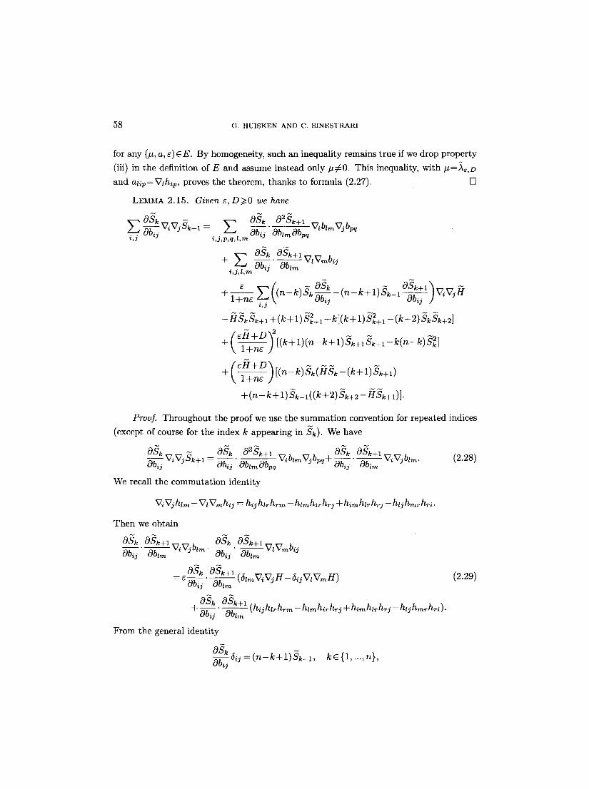
58 G. HUISKEN AND C. SINESTR.ARI
for any (#, a, r cE . By homogeneity, such an inequality remains true if we drop property
(iii) in the definition of E and assume instead only #50 . This inequality, with #=Ae,D
and alip=•lhip, proves the theorem, thanks to formula (2.27). []
LEMMA 2.15. Given E,D>~O we have
• blm V j bpq OblmOb. z,3 i,j,p,q, ,rn Pq
+ ~ .~. ( (n-k)Sk-~i j - (n-k+l)Sk-1--~- i j )WiVjH
- g s k Sk+l + (k+ 1) $2+1 § ]g[(k § 1) Sk2+1 -- (k§ Sk Sk-+-2]
+ (e~I + D ~2[(k + l ) (n-k + l )Sk+l S k _ l - k ( n - k ) S2] \ l + n s ]
+ ( t H + V ~ [(n-k) Sk(HSk-(k+l)Sk+l) \ l+n~ ]
+ ( n - k + 1) Sk-1 ((k+ 2) Sk+2 - -HSk+ 1 )1.
Proof. Throughout the proof we use the summation convention for repeated indices (except of course for the index k appearing in Sk). We have
~ V~V3b~. (2.28) O~k O~k+l
Obij cObij pq
We recall the commutation identity
Vi Vj htm- Vt Vm h~j = hij ht~ h~m - htm hi~ h~j + him hl~ h~j - htj hm~ h~i.
Then we obtain
OSk.-- O~k+ 1 ViVjbl m_ OSk. OSk+l VtVrnbij Obij Obtm Obij Obtm
OSk OSk+l (S lmViVjg-s i jV lVmg) (2 .29 ) = ~ Ob~j Oblm
OSk OSk+l (hijht~h~m- htmhi~h~j +himht~h~j - hljhm~h~i). Obij Oblm
From the general identity
OSksi j=(n-k+l lSk_l k e {1,...,n}, Obij
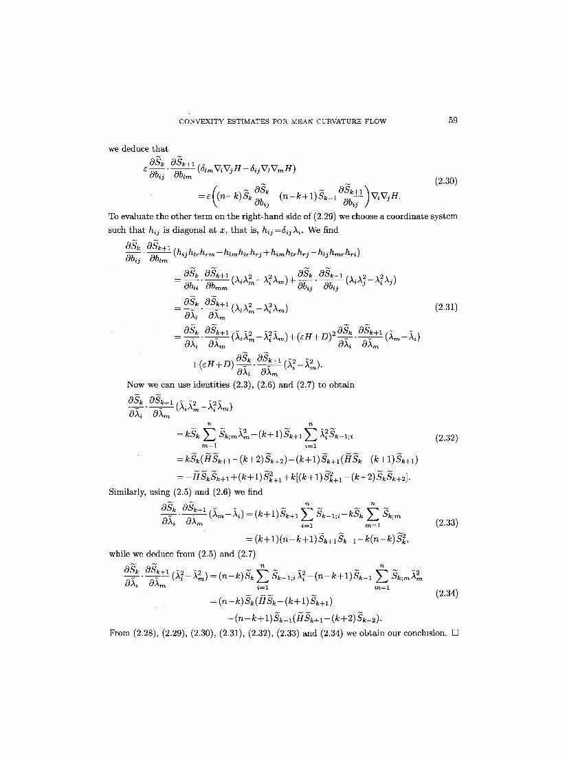
CONVEXITY ESTIMATES FOR MEAN CURVATURE FLOW 59
we deduce that
o~ e Obi~
OSk+l (6zmV~VjH- 6ijV1VmH) Ob~m
(2.30) / ~ OSk N OSk+l "~"X7.H =r ~-(n-k+l)Sa.,~j- i j ) vi .3 �9
To evaluate the other term on the right-hand side of (2.29) we choose a coordinate system
such that h~ is diagonal at x, that is, hi j=6i jAi . We find
OSk OSk+l (hij hzrh,-m - hzmhirhrj-t- himhlrhrj - hlj h,~,-h,~i) Ob~j Obzm
-Oh. Obm.~ ~ Oh,5 (:":'~-~f)'J) = os~os~+,= ( ~ , ~ - g ~ m ) (2.3,)
OA~ OA~ ogk. ogk+, (ira- i,) = O~kOA~ .OSk+oAm,(iii2_i2Xml+(EH+D)2_~i 0ira
~ og~+, (&-a,,). + ( e l l + D ) oA.~ "2 -2
Now we can use identities (2.3), (2.6) and (2.7) to obtain
=kSk s Sk;m~2--(kH-1)Sk+l s ~2Sk-1;i (2.32) m=l i=1
= kSk (HSk+l -- (k-F 2)Sk+2) -- (k-4-1) Sk+l (HSk - ( k+ 1)Sk+l)
= - H S k S k + , + (k+ 1) Sk2+, + k[(k+ 1) g~+l - (k+2) Sk gk+2].
Similarly, using (2.5) and (2.6) we find
O~k OSk+l (~m--~i) (k-4-1)Sk+l s Sk-1;i--kSk s Sk;m 0)~i 0)~m i=1 m=l (2.33)
= ( k + l ) ( n - k + l ) S k + l S k _ l - k ( n - k ) S 2,
while we deduce from (2.5) and (2.7)
O~k 0~k+1 (A2-A~)=(n-k)Sk s - -2_(n_k+l)~k_, s Sk',,~ ~2 = Sk-1;i )~i , OAi Ohm i = i m = l
= ( n - k ) S k ( H S k - ( k + l ) ' 3 k + l ) (2.34)
- ( n - k + l.),.~k_ 1 (.H,~k+ 1 - ( k + 2 ) Sk+~)-
From (2.28), (2.29), (2.30), (2.31), (2.32), (2.33) and (2.34) we obtain our conclusion. []
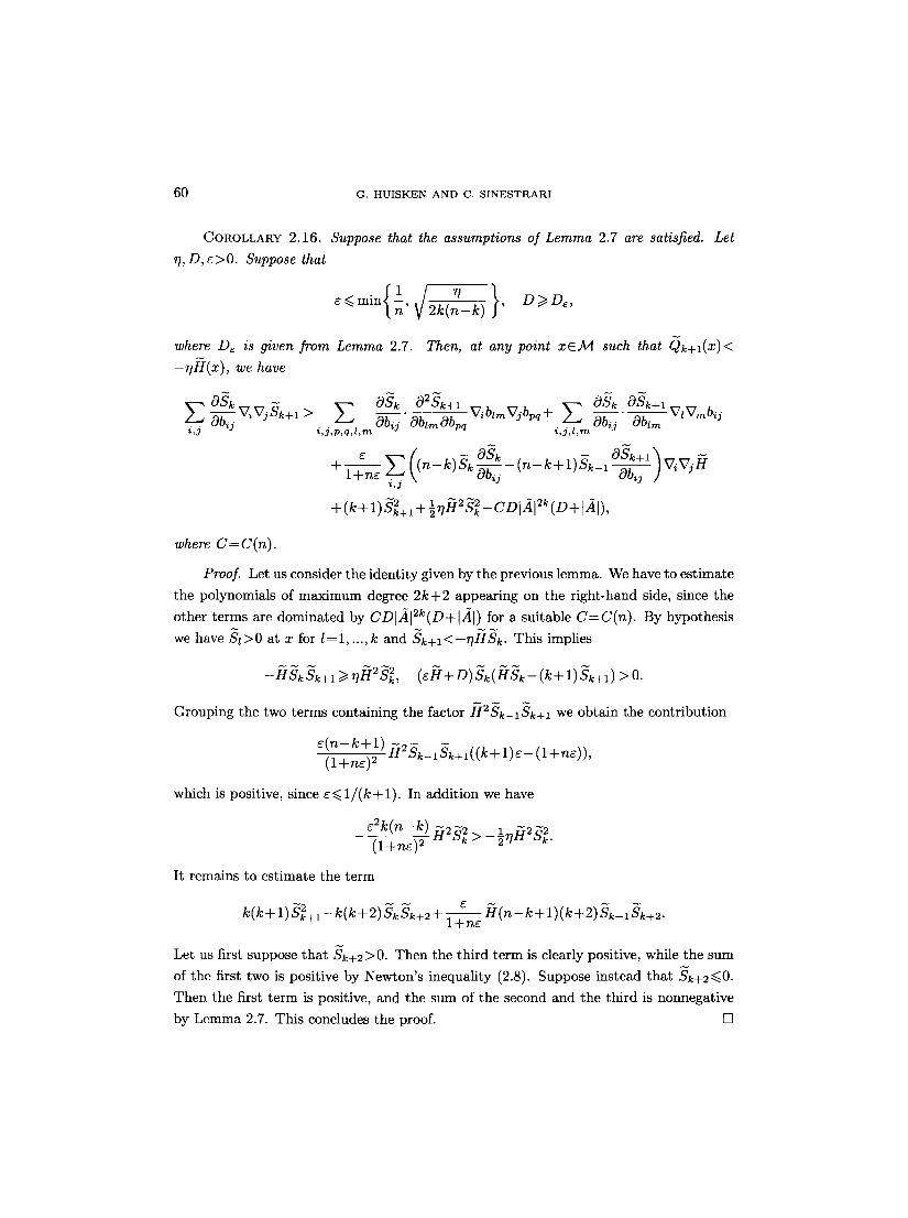
60 G. H U I S K E N AND C. S I N E S T R A R I
COROLLARY 2.16. Suppose that the assumptions of Lemma 2.7 are satisfied. Let ~, D, c>0. Suppose that
where D~ is given from Lemma 2.7. Then, at any point xEA4 such that Qk+l(x)<
- ~ I ( x ) , we have
>--: v'b mvjb'q+ 0bj i , j ~,3,p,q,~,m i , j , l , m
(( n- E k) Sk ~ - - ( n - k + l ) S k _ l --~-~j] V, VjH z,J
+(k+ ~2 ~ -2 -2 1)Sk+l+ ~ H Sk-CD]AI2k(D+tAI),
where C=C(n).
Proof. Let us consider the identity given by the previous lemma. We have to estimate
the polynomials of maximum degree 2k+2 appearing on the right-hand side, since the
other terms are dominated by CDl~l[2k(D+lA[) for a suitable C=C(n). By hypothesis
we have St>0 at x for l : l , . . . , k and Sk+I<-~?HSk. This implies
-HSkSk+I >1 ~]~I2S 2, (e~I+D)Sk(HSk-(k+l)Sk+l) > O.
Grouping the two terms containing the factor H2Sk_ISk+I we obtain the contribution
r k+ 1) ~2~k_ 1Sk+l((k+ 1)e- (1 + he)), ( l+ne) 2
which is positive, since E<~l/(k+l). In a~ldition we have
1 ~ 2 ~ 2 ~2k(n- k) ~i2~ 2 > _ ~,l~ ~k" (l+nc) 2
It remains to estimate the term
k(k + 1) ~+~ - k(k +2) ~ ~+2 + ~ ~ ( ~ - k + 1)(k + 2) ~ _ , ~+2. I d-hE
Let us first suppose that Sk+2 >0. Then the third term is clearly positive, while the sum
of the first two is positive by Newton's inequality (2.8). Suppose instead that Sk+2~<0.
Then the first term is positive, and the sum of the second and the third is nonnegative
by Lemma 2.7. This concludes the proof. []
C O N V E X I T Y E S T I M A T E S F O R M E A N C U R V A T U R E F L O W 61
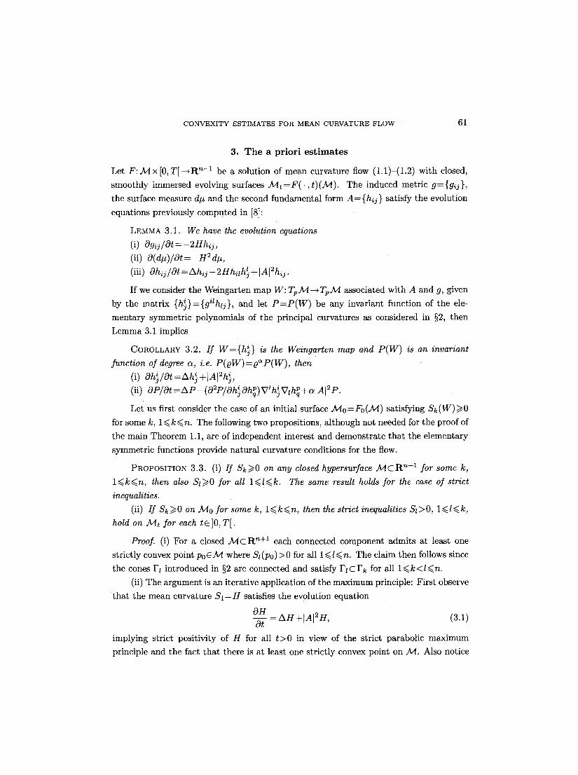
3. T h e a pr ior i e s t i m a t e s
Let F:.s x [0,T[--,R n+l be a solution of mean curvature flow (1.1)-(1.2) with closed,
smoothly immersed evolving surfaces J~4t=F(. ,t)(.t~4). The induced metric g={gij},
the surface measure dtt and the second fundamental form A={hi j} satisfy the evolution
equations previously computed in [8]:
LEMMA 3.1. We have the evolution equations
(i) Ogij/Ot=-2Hhij , (ii) O(d#)/Ot=-H2d#,
(iii) Ohiy/Ot =Ahij - 2Hhilh~ + ]A]2hq.
If we consider the Weingarten map W: TpA4--*TpAd associated with A and g, given
by the matrix {h}}={giZhtj}, and let P = P ( W ) be any invariant function of the ele-
mentary symmetric polynomials of the principal curvatures as considered in w then
Lemma 3.1 implies
COROLLARY 3.2. / f W={h~} is the Weingarten map and P(W) is an invariant
function of degree a, i.e. P(QW)=Q~P(W), then (i) Oh}/Ot=Ah} +]AI2h}, (ii) OP/Ot=AP-(O2p/Oh}OhP)VIh~VlhP+~]A]2P.
Let us first consider the case of an initial surface A/10=F0(A/t) satisfying Sk(W)>~O
for some k, 1 ~< k ~ n. The following two propositions, although not needed for the proof of
the main Theorem 1.1, are of independent interest and demonstrate that the elementary
symmetric functions provide natural curvature conditions for the flow.
PROPOSITION 3.3. (i) If Sk>~O on any closed hypersurface A d c R n+l for some k,
l<.k~n, then also Sz>~O for all l<.l<~k. The same result holds for the case of strict
inequalities.
(ii) If Sk >~O on Ado for some k, l ~ k ~ n, then the strict inequalities Sl>0, l <~ l <~ k,
hold on M t for each tE]0, T[.
Proof. (i) For a closed A 4 c R n+l each connected component admits at least one
strictly convex point P0 E A4 where S1 (Po)> 0 for all 1 ~< l ~< n. The claim then follows since
the cones Fz introduced in w are connected and satisfy F I c F k for all l<~k<l<.n.
(ii) The argument is an iterative application of the maximum principle: First observe
t h a t the mean curvature S I = H satisfies the evolution equation
OH Ot - AH+IA]2H, (3.1)
implying strict positivity of H for all t > 0 in view of the strict parabolic maximum
principle and the fact that there is at least one strictly convex point on ~4. Also notice
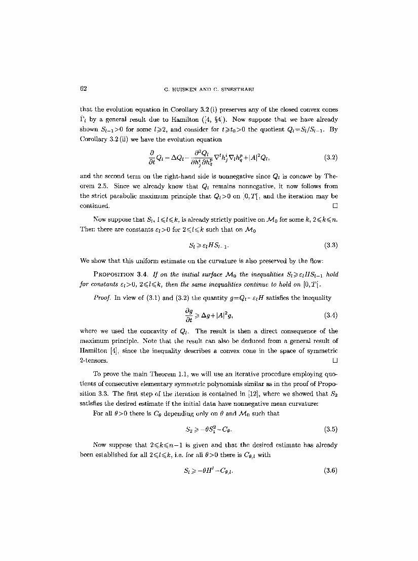
62 G. H U I S K E N A N D C. S I N E S T R A R I
that the evolution equation in Corollary 3.2 (i) preserves any of the closed convex cones
Fz by a general result due to Hamilton ([4, w Now suppose that we have already
shown S l - l > 0 for some l~>2, and consider for t~>t0>0 the quotient Qz=Sl/Sl_l. By
Corollary 3.2 (ii) we have the evolution equation
02Ql Vlh~ VthP +lAI2Qz, (3.2) O Qt = AQt i ~ Ohj Ohq
and the second term on the right-hand side is nonnegative since Qt is concave by The-
orem 2.5. Since we already know that Qt remains nonnegative, it now follows from
the strict parabolic maximum principle that Qt >0 on ]0, T[, and the iteration may be
continued. []
Now suppose that St, l<<.l<~k, is already strictly positive on A4o for some k, 2<~k<.n.
Then there are constants et >0 for 2<~t<~k such that on A4o
St >~ EzHSt-1. (3.3)
We show that this uniform estimate on the curvature is also preserved by the flow:
PROPOSITION 3.4. If on the initial surface Ado the inequalities St>>.EtHSt_I hold
for constants r 2<<.l <<.k, then the same inequalities continue to hold on [0, T[.
Proof. In view of (3.1) and (3.2) the quantity g = Q t - E t H satisfies the inequality
Og -~ >1 Ag+IAI2 g, (3.4)
where we used the concavity of Qt. The result is then a direct consequence of the
maximum principle. Note that the result can also be deduced from a general result of
Hamilton [4], since the inequality describes a convex cone in the space of symmetric
2-tensors. []
To prove the main Theorem 1.1, we will use an iterative procedure employing quo-
tients of consecutive elementary symmetric polynomials similar as in the proof of Propo-
sition 3.3. The first step of the iteration is contained in [12], where we showed that $2
satisfies the desired estimate if the initial data have nonnegative mean curvature:
For all 0>0 there is Ca depending only on 0 and Ado such that
$2 >>. -OS~-Co. (3.5)
Now suppose that 2<<.k<<.n-1 is given and that the desired estimate has already
been established for all 2<<.l<~k, i.e. for all 0>0 there is C0,z with
St >~ -OH z -Co, t. (3.6)
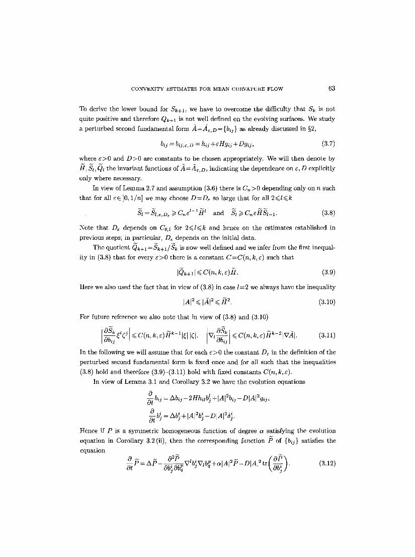
CONVEXITY ESTIMATES FOR MEAN CURVATURE FLOW 63
To derive the lower bound for Sk+l, we have to overcome the difficulty that Sk is not
quite positive and therefore Qk+l is not well defined on the evolving surfaces. We study
a perturbed second fundamental form -4=f~,D = {b~j} as already discussed in w
b~j = bij;~,D = h~j +~Hgij + Dgij, (3.7)
where e > 0 and D > 0 are constants to be chosen appropriately. We will then denote by
H, Sz, Qz the invariant functions of A=fi,~, D, indicating the dependence on e, D explicitly
only where necessary.
In view of Lemma 2.7 and assumption (3.6) there is Cn >0 depending only on n such
that for all EC ]0, 1/n] we may choose D=D~ so large that for all 2<~l<~k
St =Sz,~,D~ ~> Cnc ' - l ~ z and S, ~> Cnr (3.8)
Note that D~ depends on Co, l for 2<~l<~k and hence on the estimates established in
previous steps; in particular, DE depends on the initial data.
The quotient (~k+l =Sk+l/Sk is now well defined and we infer from the first inequal-
ity in (3.8) that for every e>0 there is a constant C=C(n, k, ~) such that
[~)k+l I ~< C(n, k, E)~I. (3.9)
Here we also used the fact that in view of (3.8) in case l=2 we always have the inequality
iA[2 • [~[2 < ~2. (3.10)
For future reference we also note that in view of (3.8) and (3.10)
a~k ~ i(j <C(n,k,r162 ' V z ~ i j <~C(n,k,e)Hk-2lVfl I. (3.11)
In the following we will assume that for each r the constant D~ in the definition of the
perturbed second fundamental form is fixed once and for all such that the inequalities
(3.8) hold and therefore (3.9)-(3.11) hold with fixed constants C(n, k, e). In view of Lemma 3.1 and Corollary 3.2 we have the evolution equations
0 b.. = Abij - 2ghi~b} + IAl2b~j -DlA[2gij, Ot ~3
0 - - Ab} +]A] b~-DIA I ~- ot b} = i 2 i 2
Hence if P is a symmetric homogeneous function of degree a satisfying the evolution
equation in Corollary 3.2 (ii), then the corresponding function /B of {b~j} satisfies the
equation
0 ~ A P 02P Vlb}VzbP+alAI2P-DIA]2tr -~j -~P = Ob~O~ . (3.12)
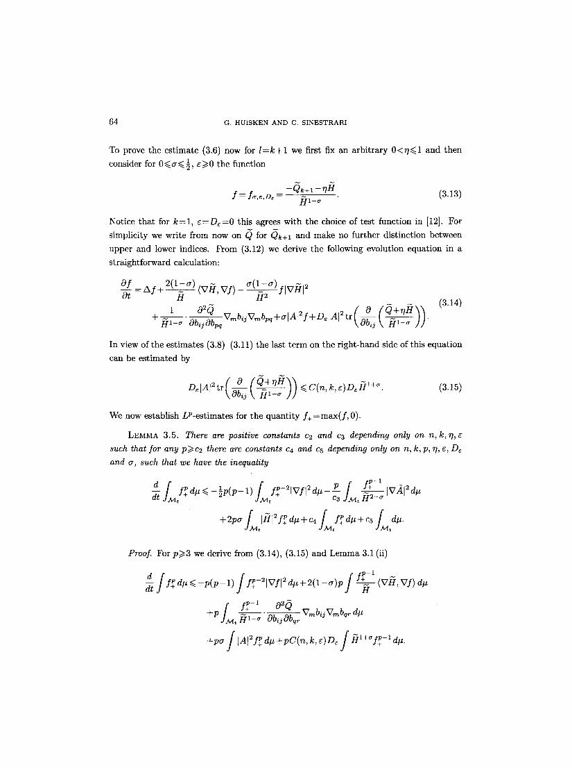
64 G. HUISKEN AND C. SINESTRARI
To prove the estimate (3.6) now for l = k + l we first fix an arbitrary 0<rl~<l and then
consider for 0~<a~< �89 e>~0 the function
-Qk+l - r /H (3.13) f = f~,e,D,-- fft1_ ~
Notice that for k = l , e=De=O this agrees with the choice of test function in [12]. For
simplicity we write from now on O for Q)k+l and make no further distinction between
upper and lower indices. From (3.12) we derive the following evolution equation in a
straightforward calculation:
( 0 ( ( ~ + r p ~ (3.14) 1 020 Vmb, jVmbpq+alAi2f+D~lAi2t r ~ \ ~ / / "
ffIl-~ ObijObpq
In view of the estimates (3.8)-(3.11) the last term on the right-hand side of this equation
can be estimated by
D d A l 2 t r ( s ( O + Y ~ l ~ <~ / / (3.15)
We now establish LP-estimates for the quantity f+=max(f , 0).
LEMMA 3.5. There are positive constants c2 and c3 depending only on n, k, rhe
such that for any p>~c2 there are constants ca and c5 depending only on n, k, p, rh e, D~
and a, such that we have the inequality
d--t fP+ dp <. - �89 1) y~+-21WI2 d~-P t t C3 t ffX2--a
Proof. For p~>3 we derive from (3.14), (3.15) and Lemma 3.1 (ii)
d f+p-1 f f f - lvfl 2(1- )p f <vh, vf/d --dt J fP+ d# <<. , p ( p - 1) - - i f -
F+ -1 O2Q. /A4 Vmbij Vrnbqr d# + P , f fIl-~ " Ob~jObq~
+pa / IA,2fP+ d.+pC(n,k,e)D~ f ~II+~fP+-~ d..
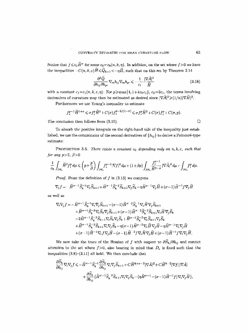
CONVEXITY ESTIMATES FOR MEAN CURVATURE FLOW 65
Notice that f<~coffI ~ for some co=c0(n, k, 7). In addition, on the set where f > 0 we have
the inequalities -C(n, k, r <-r//~, such that on this set by Theorem 2.14
020 1 Iwil ObijOba~ VmbijVmbqr <~ Cl ffI (3.16)
with a constant c~=cl(n, k, e, r/). For p~>max{4, I+4coc~}, c3=2c~, the terms involving
derivatives of curvature may then be estimated as desired since [VA[2~> (l/n)[V/~[ 2.
Furthermore we use Young's inequality to estimate
f p - - l j ~ l + a < crfV+ffi2 +C(a)fp-2/(1-,r) << afph2 +C(a) fp+ +C(a,p).
The conclusion then follows from (3.10). []
To absorb the positive integrals on the right-hand side of the inequality just estab-
lished, we use the commutator of the second derivatives of {hij } to derive a Poincar~-type
estimate:
PROPOSITION 3.6. There exists a constant c6 depending only on n, k, E, such that for any p>2, /3>0
i f.a4tffi2f~ dlz<<. (p+ ~) [ fP-~lVf]2d#+ ( l+ ,p ) f .M fp-1 'VA]9~d# + [ f+P d#. t H 2-a C6 d J~t J ~ t
Proof. From the definition of f in (3.13) we compute
Vjf = - H ' - ' S ; ~ V3 S~+1 + H " - 1 S ; % ~ V3 S~ - , H ~ - ~ V3H+ ( ~ - 1) H - g V 3 H
as well as
-- 2~IC~- l ~k3 Sk + l Vi Sk V j S k -~ g c r - l S k 2 Vi Sk + l V j S k
+ ( a - 1) H - 1Vi f VjH - ( a - 1)H-2f ViHVjH+ (cr- 1) H - ' f V, Vj H.
We now take the trace of the Hessian of f with respect to CgSk/Obij and restrict
attention to the set where f > 0 , also bearing in mind that D~ is fixed such that the
inequalities (3.8)-(3.11) all hold. We then conclude that
~cr--1 ~- -10Sk ~ ~k+a--3 - 2 --k--2 OSk ViVj f <<.-H S k ~ViV~Sk+I+CH IVAI + C H IWl IWil Obij
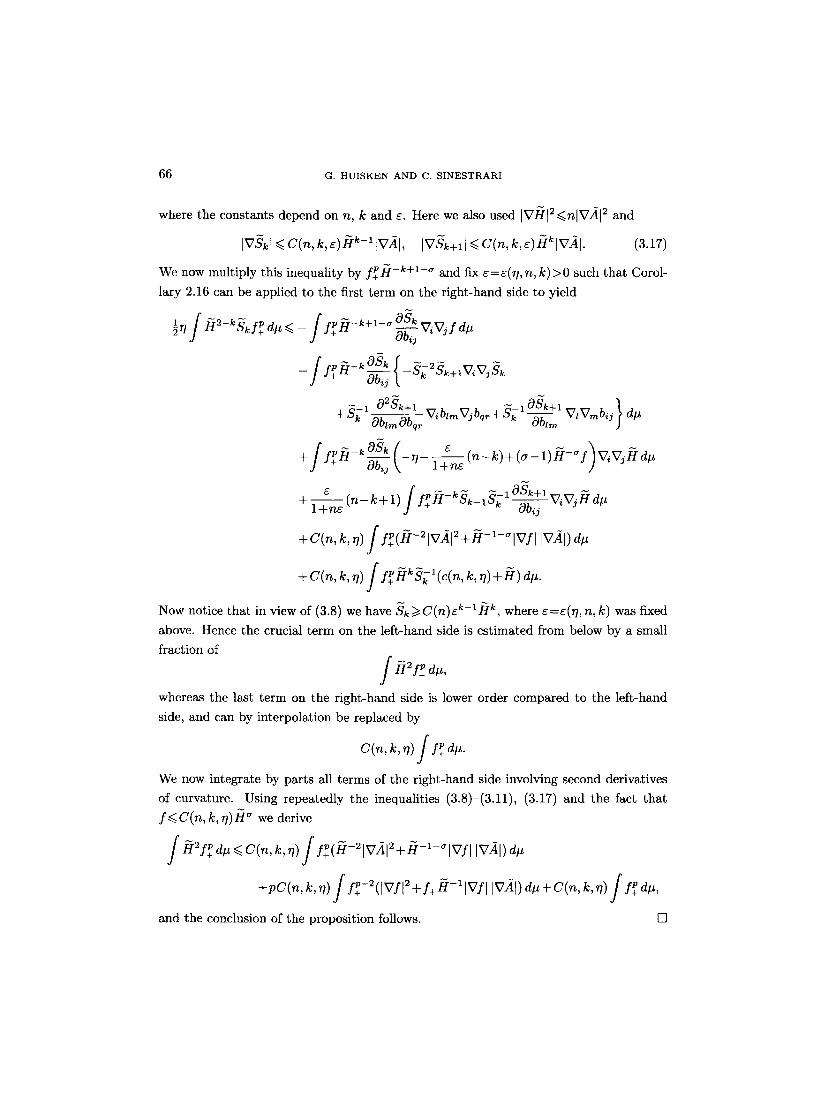
66 G. H U I S K E N AND C. SINESTI%ARI
where the constants depend on n, k and ~. Here we also used IV_I~I2~<nlVAI 2 and
IVSkl~C(n,k,-c)~Ik-lIVAI, IV"3k+ll<. C(n,k,~)I-IklVA[. (3.17)
We now multiply this inequality by fP+.~I -k+l-" and fix ~=~(17, n, k)>0 such that Corol-
lary 2.16 can be applied to the first term on the right-hand side to yield
--1 02Sk+1 - lOSk+lvzvmb~j~d# +Sk Ob~mObq,. ViblmVjbq,.+S[ Oblm
, #
+ i :PH- ~-~j - kOSk(--I 7 -- ~ ~ (n-k)+(a-l)~I- ' f)ViV, FId#
p - k- ~ l OSk+l + V 4 - ~ ( n - k + I ) S s ' + H - Sk_,S; ~ 'V, V3~Id.
+ C(n, k, 17) S /+p(~ -2 ivAl ~ +~-1-~ IV/I IvAI) d#
+ C(n, k, r#) i :+ ~: ~ : ( <(,,, '<, ,,) + ~ ) dis.
Now notice that in view of (3.8) we have Sk>~C(n)Ek-l~I k, where ~----~(17, n, k) was fixed
above. Hence the crucial term on the left-hand side is estimated from below by a small
fraction of
f P72fP+ d#,
whereas the last term on the right-hand side is lower order compared to the left-hand
side, and can by interpolation be replaced by
k, V) i / + , dis. C(n,
We now integrate by parts all terms of the right-hand side involving second derivatives
of curvature. Using repeatedly the inequalities (3.8)-(3.11), (3.17) and the fact that
f <~ C(n, k,r#)tI <~ we derive
i ~s~s~* dis <~ C(n,k, 'D i f+'(~-~IVAI~ +H-I-<,IVfl IVAI) dis
+pC(n, k, 17) J f+p-2(ivSl2 + f+ i~--1 iVf i IV~I ) d# + C(n, k, 17) i fP+ dis,
and the conclusion of the proposition follows. []
C O N V E X I T Y E S T I M A T E S F O R M E A N C U R V A T U R E F L O W 67
COROLLARY 3.7. There are constants c7 and Cs depending only on n, k, ~ and the
initial data such that for p>~cT, O~a~esp -W2 there is a uniform bound
/ fP+d#~c9 on [0, T[, t
depending only on n, k, ~, a, p and Ado.
Proof. From Lemma 3.5 and Proposition 3.6 with j3=p -1/2 we infer that for p, a as
above
-~ / ff+ p < C / fP+ d# + C / d#
with constants depending on n, k, p, ~, a and M0. This yields the desired estimate since
T is bounded in terms of the diameter of the initial surface. []
Having established the LP-bound for a=O(p -1/2) the proof of the sup-bound for f
proceeds exactly as in [12], compare also [14] and [8]. This establishes the next step in
the iteration on k according to Lemma 2.8, and completes the proof of the main result
in Theorem 1.1. []
Remark 3.8. It was shown by Smoczyk in [14] that a star-shaped surface evolving by
mean curvature satisfies the bound on the scalar curvature corresponding to the first step
in our iteration. He also proved that , for such surfaces, the uniform bounds H~>-C1 and
IAI2<~C2H2+C3 hold for suitable constants Ci. It is easily checked that our Lemmas 2.7
and 2.8 are still valid (with a different choice of the constants) replacing the assumption
H > 0 with these weaker bounds. Therefore, the iterative procedure of this section can
be applied, and the main results in Theorem 1.1 and Corollary 1.2 hold in the class of
star-shaped surfaces as well.
Remark 3.9. Let F: A~ • [0, T[--~ (N n+l , h) be a closed hypersurface of nonnegative
mean curvature evolving by mean curvature flow in a smooth Riemannian manifold
(N n+l, h) satisfying bounds - K 1 ~ON ~K2, IVgRiem I~L, iN >0 on its sectional curva-
ture, gradient of Riemann curvature tensor and injectivity radius respectively, similarly
as in [9]. Then the estimates in Theorem 1.1 continue to hold with constants Cmk now
also depending on the data of (N n+l, h) above, and we again conclude that singularities
of mean convex surfaces have convex blowups. To see this, first note that the mean
curvature satisfies (compare [9])
OH = A H + H (IAI2 + RicN(v ' v) ) Ot
and therefore remains nonnegative due to the parabolic maximum principle.
68 G. H U I S K E N A N D C. S I N E S T R A R I
Furthermore, the crucial evolution equation for the full second fundamental form
differs from the Euclidean case only by lower-order terms, see [9]:
O A = + ]A]2A+ + AA RiemN. A V N Riem N .
Similar lower-order terms appear in the commutator identity for the second derivatives
of the second fundamental form, and hence the additional terms in Lemma 3.5 and
Proposition 3.6 can all be estimated by
c f fr dtt,
with a constant depending on n, k, p, K1 , / (2 and L. The proof then proceeds as before.
4. D e s c r i p t i o n o f s ingu la r i t i e s
Let [0, T[ be the maximal time interval where a smooth solution of the flow exists, such
that s u p ~ ]A] 2 becomes unbounded for t---~T. We assume the reader to be familiar
with the rescaling procedure described in [12], see also [6] and [5]. The new estimates
in Theorem 1.1 yield a description of type-II singularities of the flow in the case of
nonnegative mean curvature.
Let (Xk, tk) be an essential blowup sequence as in (4.2) and (4.3) of [12], and let A/lk,t
be the corresponding rescaled surfaces with limiting mean curvature flow J~4r, TER, as
described in [12, Lemma 4.4 and Theorem 4.5]. As in this reference we call a solution of
mean curvature flow (1.1) which exists for all time and moves by translation in R n+l a
translating soliton.
THEOREM 4.1. If 2~40 has nonnegative mean curvature, then any limiting flow of a
type-II singularity has convex surfaces .Mr, TE R . Furthermore, either .Mr is a strictly
convex translating soliton or (up to rigid motion) n-k k k .tct~-=R x E r , where E~ is a lower-
dimensional strictly convex translating soliton in R k + l.
Proof. The convexity of the limiting flow is for both type-I and type-II singular-
ities an immediate consequence of the a priori estimates in Theorem 1.1. To obtain
the splitting result we apply the strict maximum principle for symmetric 2-tensors of
Hamilton [4, Lemma 8.2] to the evolution of the nonnegative second fundamental form
0 hj ~ -= Ah}+lAl2h} (4.1)
on the limiting flow A//~, TER. Thus the rank of A is a constant, and the null space of A
is invariant under parallel translation and invariant in time. Using the Frobenius theorem
C O N V E X I T Y E S T I M A T E S F O R M E A N C U R V A T U R E F L O W 69
N
as in [4, w or as in [11, Theorem 5.1] we see that each .A4~ splits as an isometric product n - - k . x~k k R ~z,~, where E~ is strictly convex unless j~4~ is strictly convex itself. Finally, E~ is
a translating soliton since it is convex, solves mean curvature flow for all T E R and admits
the maximum of the mean curvature at one point at least, compare [6, Theorem 1.3]. []
We wish to point out that the splitting result can also be obtained by a successive
application of the (scalar) maximum principle to the quantities Qk, 2 <. k<~n, satisfying
the parabolic equations (3.2). The splitting dimension k is then characterised by the
relations Sn = Sn - 1 . . . . . Sk+l = 0, St > 0 when 1 ~< l ~< k.
In the case k = 1 the only translating soliton is the "grim reaper" durve x = log cos y+t, and in higher dimensions it is known that there are rotationally symmetr ic translating
solitons. It is an open problem whether in higher dimensions there are other translating
solitons, convex or of positive mean curvature.
Acknowledgements. The second author thanks the SFB 382 and the Forschungskreis
Mathemat ik at the University of Tfibingen for the support while this paper was written.
70 G. HUISKEN AND C. SINESTRARI
R e f e r e n c e s
[1] ANDREWS, B., Contraction of convex hypersurfaces in Euclidean space. Calc. liar. Partial Differential Equations, 2 (1994), 151-171.
[2] CAFFARELLI, a., NIRENBERG, L. • SPRUCK, J., The Dirichlet problem for nonlinear second order elliptic equations, III: ~unctions of the eigenvalues of the Hessian. Acta Math., 155 (1985), 261-301.
[3] G.~RDING, L., An inequality for hyperbolic polynomials. J. Math. Mech., 8 (1959), 957-965. [4] HAMILTON, R.S., Four-manifolds with positive curvature operator. J. Differential Geom.,
24 (1986), 153-179. [5] - - The formation of singularities in the Ricci flow, in Surveys in Differential Geometry,
Vol. II (Cambridge, MA, 1993), pp. 7-136. Internat. Press, Cambridge, MA, 1993. [6] - - Harnack est imate for the mean curvature flow. J. Differential Geom., 41 (1995), 215-226. [7] HARDY, G.H., LITTLEWOOD, J.E. ~ POLYA, G., Inequalities. Cambridge Univ. Press,
Cambridge, 1934. [8] HUISKEN, G., Flow by mean curvature of convex surfaces into spheres. J. Differential
Geom., 20 (1984), 23~266. [9] - - Contracting convex hypersurfaces in Riemannian manifolds by their mean curvature.
Invent. Math., 84 (1986), 463-480. [10] - - Asymptot ic behaviour for singularities of the mean curvature flow. J. Differential Geom.,
31 (1990), 285-299. [11] - - Local and global behaviour of hypersurfaces moving by mean curvature. Proc. Sympos.
PureMath., 54 (1993), 175-191. [12] HUISKEN, G. ~ SINESTRARI, C., Mean curvature flow singularities for mean convex sur-
faces. Calc. Vat. Partial Differential Equations, 8 (1999), 1-14. [13} MARCUS, M. &= LOPES, L., Inequalities for symmetric functions and Hermitian matrices.
Canad. J. Math., 9 (1957), 305-312. [14] SMOCZYK, K., Starshaped hypersurfaces and the mean curvature flow. Manuscripta Math.,
95 (1998), 225-236.
GERHARD HUISKEN Mathematisches Inst i tut Universitgt Tiibingen Auf der Morgenstelle 10 DE-72076 Tiibingen Germany gerhard.huisken@uni-t uebingen.de
CARLO SINESTRARI Dipart imento di Matemat ica Universit~ di Roma "Tor Vergata" Via della Ricerca Scientifica IT-00133 Rome Italy [email protected]
Received June 4, 1998 Received in revised form April 19, 1999