convolutional neural network for sentence … · convolutional neural network for sentence...
TRANSCRIPT
Convolutional Neural Network forSentence Classification
by
Yahui Chen
A thesispresented to the University of Waterloo
in fulfillment of thethesis requirement for the degree of
Master of Mathematicsin
Computer Science
Waterloo, Ontario, Canada, 2015
c� Yahui Chen 2015
I hereby declare that I am the sole author of this thesis. This is a true copy of the thesis,including any required final revisions, as accepted by my examiners.
I understand that my thesis may be made electronically available to the public.
ii
Abstract
The goal of a Knowledge Base–supported Question Answering (KB-supported QA) systemis to answer a query natural language by obtaining the answer from a knowledge database,which stores knowledge in the form of (entity, relation, value) triples. QA systems under-stand questions by extracting entity and relation pairs. This thesis aims at recognizingthe relation candidates inside a question. We define a multi-label classification problem forthis challenging task. Based on the word2vec representation of words, we propose two con-volutional neural networks (CNNs) to solve the multi-label classification problem, namelyParallel CNN and Deep CNN. The Parallel CNN contains four parallel convolutional layerswhile Deep CNN contains two serial convolutional layers. The convolutional layers of boththe models capture local semantic features. A max over time pooling layer is placed onthe top of the last convolutional layer to select global semantic features. Fully connectedlayers with dropout are used to summarize the features. Our experiments show that thesetwo models outperform the traditional Support Vector Classification (SVC)–based methodby a large margin. Furthermore, we observe that Deep CNN has better performance thanParallel CNN, indicating that the deep structure enables much stronger semantic learningcapacity than the wide but shallow network.
iii

Acknowledgements
I would like to thank all the people who made this possible. First and foremost, I wantto express profound gratitude towards my supervisor Dr. Ming Li for his support. Hisinvaluable detailed advices on project and thesis encourage me a lot. Second, I would liketo thank Dr. Pascal Poupart. He provides insight and expertise that assisted my thesis.Third, I would like to thank Dr. Chrysanne Di Marco and Dr. Khuzaima Daudjee to readmy thesis and to provide valuable advices. Finally, My sincere thanks go to my father andall my friends for their encouragement and support.
iv
Dedication
This is dedicated to my family.
v
Table of Contents
List of Tables ix
List of Figures x
1 Introduction 1
1.1 Background and Motivation . . . . . . . . . . . . . . . . . . . . . . . . . . 1
1.2 Problem Definition . . . . . . . . . . . . . . . . . . . . . . . . . . . . . . . 2
1.3 Contributions . . . . . . . . . . . . . . . . . . . . . . . . . . . . . . . . . . 2
1.4 Thesis Organization . . . . . . . . . . . . . . . . . . . . . . . . . . . . . . . 3
2 Background 4
2.1 Deep Neural Network . . . . . . . . . . . . . . . . . . . . . . . . . . . . . . 4
2.1.1 Convolutional Neural Network . . . . . . . . . . . . . . . . . . . . . 4
2.1.2 Recurrent Neural Network . . . . . . . . . . . . . . . . . . . . . . . 5
2.1.3 Recursive Neural Network . . . . . . . . . . . . . . . . . . . . . . . 7
2.2 Motivation and History . . . . . . . . . . . . . . . . . . . . . . . . . . . . . 8
2.3 Basic Assumption . . . . . . . . . . . . . . . . . . . . . . . . . . . . . . . . 8
2.4 Review of Discrete Convolution Definition . . . . . . . . . . . . . . . . . . 8
2.5 Volumes of Neurons . . . . . . . . . . . . . . . . . . . . . . . . . . . . . . . 9
2.6 Architecture . . . . . . . . . . . . . . . . . . . . . . . . . . . . . . . . . . . 9
2.6.1 Convolutional Layer . . . . . . . . . . . . . . . . . . . . . . . . . . 9
vi
2.6.2 Pooling Layer . . . . . . . . . . . . . . . . . . . . . . . . . . . . . . 12
2.6.3 Fully Connected Layer . . . . . . . . . . . . . . . . . . . . . . . . . 13
2.6.4 Dropout . . . . . . . . . . . . . . . . . . . . . . . . . . . . . . . . . 14
2.6.5 Activation Function and Cost Function . . . . . . . . . . . . . . . . 15
2.6.6 Common CNN Architectures . . . . . . . . . . . . . . . . . . . . . . 17
3 Related Work 18
3.1 Single–Convolutional–Layer CNNs . . . . . . . . . . . . . . . . . . . . . . . 18
3.2 Multi–Convolutional–Layer CNNs . . . . . . . . . . . . . . . . . . . . . . . 20
4 Dataset and Environment 23
4.1 Dataset . . . . . . . . . . . . . . . . . . . . . . . . . . . . . . . . . . . . . 23
4.1.1 Data Format . . . . . . . . . . . . . . . . . . . . . . . . . . . . . . 23
4.1.2 Answerable Queries Coverage . . . . . . . . . . . . . . . . . . . . . 24
4.2 Tool and Environment . . . . . . . . . . . . . . . . . . . . . . . . . . . . . 24
4.2.1 word2vec . . . . . . . . . . . . . . . . . . . . . . . . . . . . . . . . . 24
4.2.2 NER . . . . . . . . . . . . . . . . . . . . . . . . . . . . . . . . . . . 25
4.2.3 CUDA . . . . . . . . . . . . . . . . . . . . . . . . . . . . . . . . . . 25
4.2.4 Python Libraries . . . . . . . . . . . . . . . . . . . . . . . . . . . . 25
4.2.5 Spelling Corrector . . . . . . . . . . . . . . . . . . . . . . . . . . . . 25
4.2.6 Experiment Environment . . . . . . . . . . . . . . . . . . . . . . . . 25
5 Main Results 27
5.1 Methodologies . . . . . . . . . . . . . . . . . . . . . . . . . . . . . . . . . . 27
5.1.1 Data Processing . . . . . . . . . . . . . . . . . . . . . . . . . . . . . 27
5.1.2 Multi–Label Classification . . . . . . . . . . . . . . . . . . . . . . . 30
5.1.3 Models . . . . . . . . . . . . . . . . . . . . . . . . . . . . . . . . . . 31
5.1.4 Evaluation Metrics . . . . . . . . . . . . . . . . . . . . . . . . . . . 34
vii
5.2 Experiments and Results . . . . . . . . . . . . . . . . . . . . . . . . . . . . 35
5.2.1 Baseline versus CNNs . . . . . . . . . . . . . . . . . . . . . . . . . 36
5.2.2 Parallel versus Deep CNN . . . . . . . . . . . . . . . . . . . . . . . 36
5.2.3 Further Observations . . . . . . . . . . . . . . . . . . . . . . . . . . 36
6 Conclusions 41
6.1 Summary . . . . . . . . . . . . . . . . . . . . . . . . . . . . . . . . . . . . 41
6.2 Future Work . . . . . . . . . . . . . . . . . . . . . . . . . . . . . . . . . . . 41
APPENDICES 43
A Python Implementation for Building CNNs 44
A.1 Deep CNN . . . . . . . . . . . . . . . . . . . . . . . . . . . . . . . . . . . . 44
A.2 Parallel CNN . . . . . . . . . . . . . . . . . . . . . . . . . . . . . . . . . . 45
References 46
viii
List of Tables
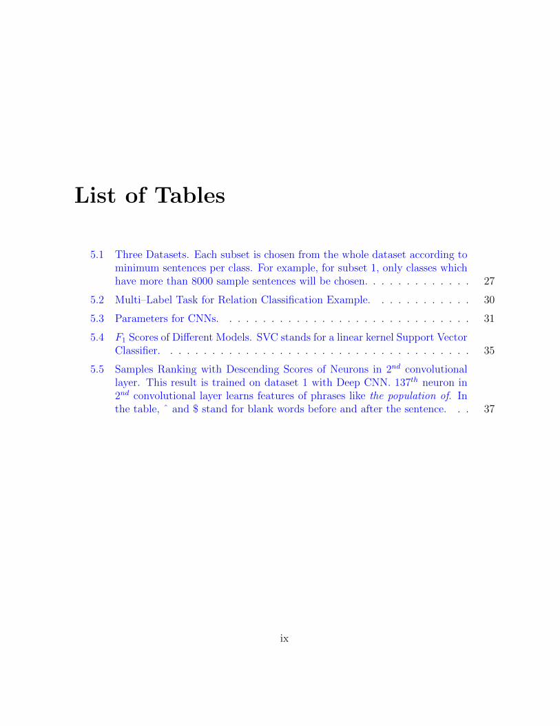
5.1 Three Datasets. Each subset is chosen from the whole dataset according tominimum sentences per class. For example, for subset 1, only classes whichhave more than 8000 sample sentences will be chosen. . . . . . . . . . . . . 27
5.2 Multi–Label Task for Relation Classification Example. . . . . . . . . . . . 30
5.3 Parameters for CNNs. . . . . . . . . . . . . . . . . . . . . . . . . . . . . . 31
5.4 F1 Scores of Di↵erent Models. SVC stands for a linear kernel Support VectorClassifier. . . . . . . . . . . . . . . . . . . . . . . . . . . . . . . . . . . . . 35
5.5 Samples Ranking with Descending Scores of Neurons in 2nd convolutionallayer. This result is trained on dataset 1 with Deep CNN. 137th neuron in2nd convolutional layer learns features of phrases like the population of. Inthe table, ˆ and $ stand for blank words before and after the sentence. . . 37
ix
List of Figures
1.1 KB-supported QA. . . . . . . . . . . . . . . . . . . . . . . . . . . . . . . . 1
2.1 Convolutional Neural Network. Neurons in CNN are locally connected withneurons in previous layer. Weights of the same filter are shared across thesame layer. . . . . . . . . . . . . . . . . . . . . . . . . . . . . . . . . . . . . 5
2.2 Recurrent Neural Network. RNN takes input sequence. Weights of hiddenunits are updated according to current input and previous weights of hiddenunits at each time step. Outputs of RNN are calculated according to currenthidden units state. . . . . . . . . . . . . . . . . . . . . . . . . . . . . . . . 6
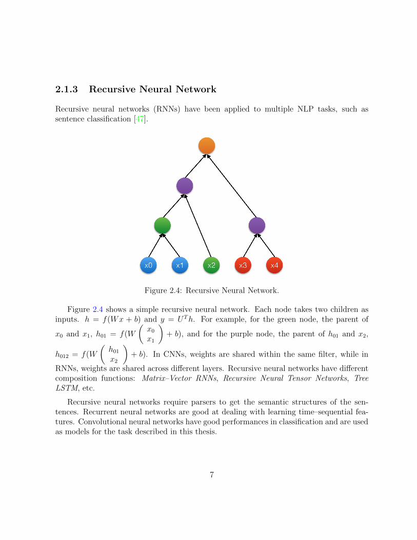
2.3 Error Surface of a Single Hidden Unit RNN [41]. . . . . . . . . . . . . . . . 6
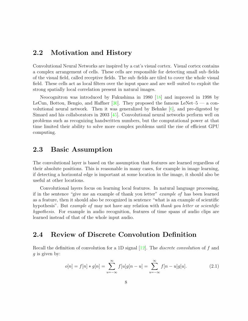
2.4 Recursive Neural Network. . . . . . . . . . . . . . . . . . . . . . . . . . . . 7
2.5 Sparse Connectivity. . . . . . . . . . . . . . . . . . . . . . . . . . . . . . . 10
2.6 Shared Weights. Connections with same colour share weights. . . . . . . . 10
2.7 Convolutional Layer [26]. . . . . . . . . . . . . . . . . . . . . . . . . . . . . 11
2.8 Pooling Layer. . . . . . . . . . . . . . . . . . . . . . . . . . . . . . . . . . . 13
2.9 Dropout. . . . . . . . . . . . . . . . . . . . . . . . . . . . . . . . . . . . . . 14
2.10 Activation Function Applied to a Neuron. . . . . . . . . . . . . . . . . . . 15
2.11 Activation Functions. This figure shows sigmoid, tanh and ReLU function.As seen from the figure, sigmoid’s output range is [0, 1], while tanh’s outputrange is [�1, 1] and ReLU’s output range is [0,+1] . . . . . . . . . . . . . 16
3.1 Neural Network for Relation Classification and Framework for ExtractingSentence Level Features [55]. In the right hand figure, WF stands for wordfeatures and PF stands for position features. . . . . . . . . . . . . . . . . . 18
x

3.2 CNN Model [44]. . . . . . . . . . . . . . . . . . . . . . . . . . . . . . . . . 19
3.3 CNN Model [51]. . . . . . . . . . . . . . . . . . . . . . . . . . . . . . . . . 19
3.4 CNN Model for Several Sentence Classification Tasks [27]. . . . . . . . . . 20
3.5 ARC–II Model [22]. . . . . . . . . . . . . . . . . . . . . . . . . . . . . . . . 20
3.6 DCNN Model for Modeling Sentence [25]. . . . . . . . . . . . . . . . . . . . 21
4.1 The Curve of Coverage of Queries Answerable and Number of Relation. . . 24
5.1 Sentence Space. Depth is one, width is the number of words in a sentence,and height is three hundred which is the dimension of word2vec. . . . . . . 28
5.2 Padding Zeros. . . . . . . . . . . . . . . . . . . . . . . . . . . . . . . . . . 29
5.3 Deep CNN. . . . . . . . . . . . . . . . . . . . . . . . . . . . . . . . . . . . 32
5.4 Parallel CNN. . . . . . . . . . . . . . . . . . . . . . . . . . . . . . . . . . . 33
5.5 Precision Recall Curves. . . . . . . . . . . . . . . . . . . . . . . . . . . . . 38
5.6 Receiver Operating Characteristic Curves. . . . . . . . . . . . . . . . . . . 39
xi
Chapter 1
Introduction
1.1 Background and Motivation
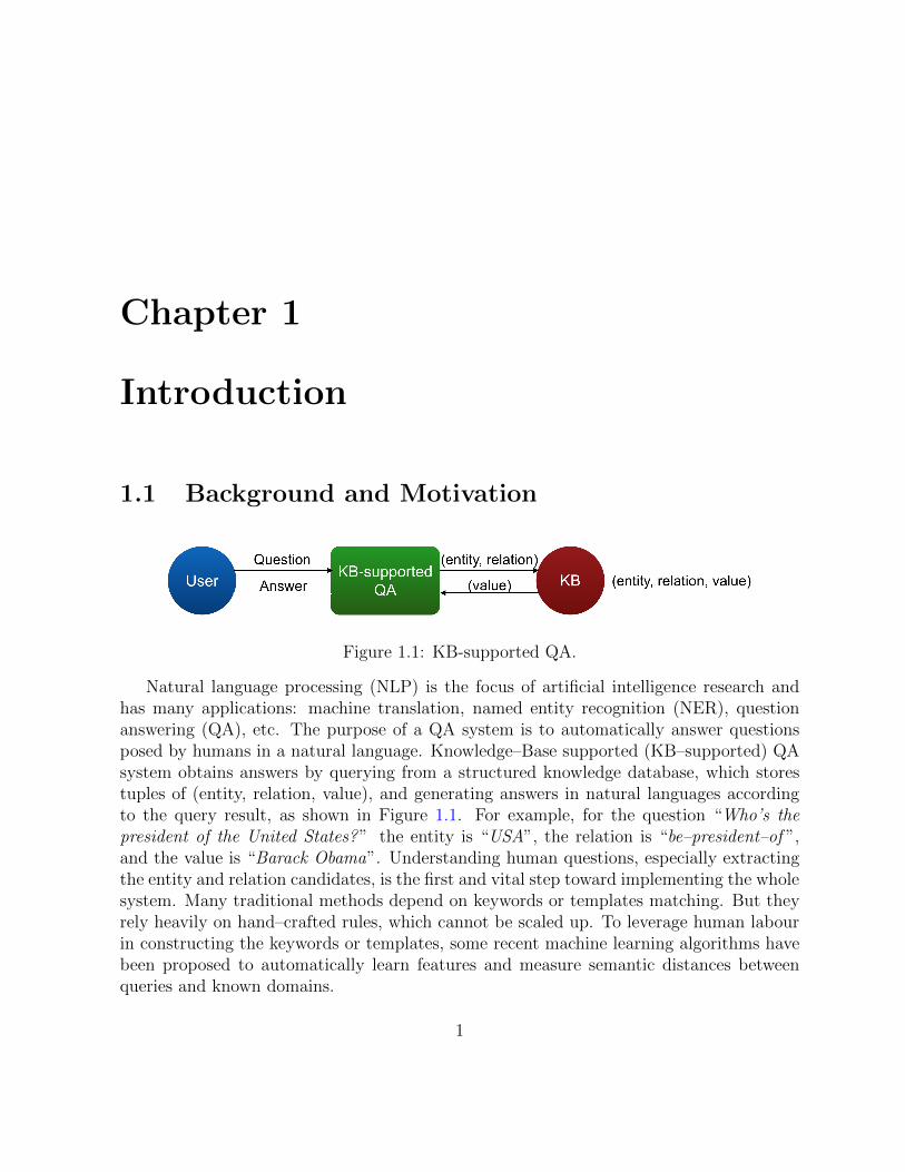
Figure 1.1: KB-supported QA.
Natural language processing (NLP) is the focus of artificial intelligence research andhas many applications: machine translation, named entity recognition (NER), questionanswering (QA), etc. The purpose of a QA system is to automatically answer questionsposed by humans in a natural language. Knowledge–Base supported (KB–supported) QAsystem obtains answers by querying from a structured knowledge database, which storestuples of (entity, relation, value), and generating answers in natural languages accordingto the query result, as shown in Figure 1.1. For example, for the question “Who’s thepresident of the United States?” the entity is “USA”, the relation is “be–president–of ”,and the value is “Barack Obama”. Understanding human questions, especially extractingthe entity and relation candidates, is the first and vital step toward implementing the wholesystem. Many traditional methods depend on keywords or templates matching. But theyrely heavily on hand–crafted rules, which cannot be scaled up. To leverage human labourin constructing the keywords or templates, some recent machine learning algorithms havebeen proposed to automatically learn features and measure semantic distances betweenqueries and known domains.
1
1.2 Problem Definition
This thesis defines a multi–label classification problem for extracting the relation candidatesfrom a question. We target a widely used question dataset [15], which is crawled fromWikiAnswer and consists of a set of questions with over 19K relations. We assume thatthese open–domain questions have only first–order relations, which we call single–relationquestions, for example, “Who’s the president of the United States?” has a first–orderrelation, but “Who’s the wife of the United States’ president?” has a second–order relation.Single–relation questions are the most commonly observed ones in QA sites [16]. However,since human expressions or understanding could be ambiguous, each question may haveseveral relation candidates, for example, “What is the primary duty of judicial branch?”has relation candidates “be–primary–responsibility–of ”, “be–primary–role–of ”, and “have–role–of ”. Thus we address the problem as recognizing the relations inside a question in amulti–label manner.
1.3 Contributions
We explore various deep learning models to solve the proposed multi–label recognition prob-lem. At the first step, we exploit the widely used word2vec [33] [35] [36] to represent eachword as a 300 dimensional vector, and the whole sentence as a matrix by stacking all theword vectors. Word2vec converts the semantic relations between words into the distanceof their vectors, for example, word2vec(‘Paris’) - word2vec(‘France’) + word2vec(‘China’)= word2vec(‘Beijing’).
Based on the matrix representation of each sentence, we propose two kinds of convolu-tional neural networks (CNNs): Parallel CNN and Deep CNN. Convolutional layers of bothnetworks can learn phrases, such as “where do . . . live”, and “the population of”. ParallelCNN is a shallow network but has multiple parallel convolutional layers. Deep CNN, onthe contrary, has multiple serial convolutional layers. Our experiments show that bothParallel and Deep CNN outperform the traditional Support Vector Classification (SVC)–based method by a large margin. Furthermore, we observe that Deep CNN has betterperformance than Parallel CNN, indicating that the deep structure enables much strongersemantic learning capacity than the wide but shallow network.
2
1.4 Thesis Organization
Section 2 mainly background knowledge of the structures and components of CNNs. Sec-tion 3 introduces recent research on CNNs for NLP tasks. Section 4 presents the dataset,tools, and environment used in this work. Section 5 describes our method and showsexperimental results. Section 6 concludes this thesis.
3

Chapter 2
Background
2.1 Deep Neural Network
Deep learning has shown powerful feature learning skills and achieved remarkable perfor-mance in computer vision (CV) [8] [43], speech recognition [11] [21], and natural languageprocessing (NLP) [9]. Deep neural network is a kind of deep learning method. The dif-ference between deep neural network (DNN) and shallow artificial neural network (ANN)is that the former contains multiple hidden layers so that it can learn more complex fea-tures. It has several variants: convolutional neural network, recurrent neural network, andrecursive neural network. DNNs have forward pass and back propagation. The parametersof networks are updated according to learning rate, cost function via stochastic gradientdescent during the back propagation. In the following, we briefly introduce the structuresof di↵erent DNNs applied in NLP tasks.
2.1.1 Convolutional Neural Network
Convolutional neural networks (CNNs) learn local features and assume that these featuresare not restricted by their absolute positions. In the field of NLP, they are applied inPart–Of–Speech Tagging (POS), Named Entity Recognition (NER) [9], etc.
Figure 2.1 shows a two–layer CNN. For the green node h0 = f(W
0
@x0
x1
x2
1
A + b) =
4
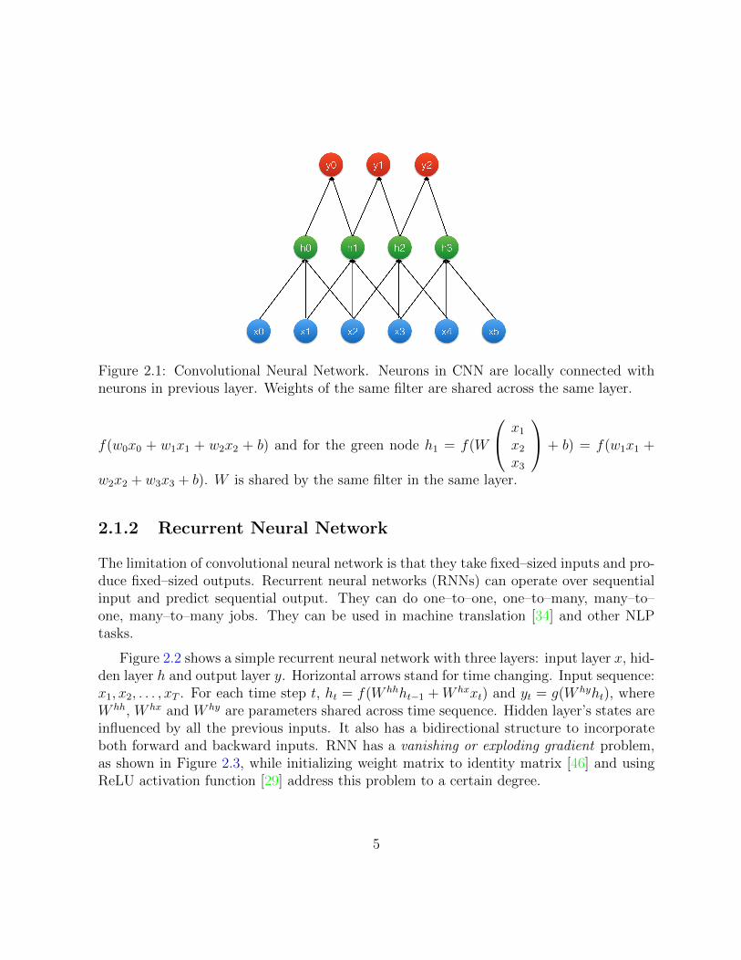
Figure 2.1: Convolutional Neural Network. Neurons in CNN are locally connected withneurons in previous layer. Weights of the same filter are shared across the same layer.
f(w0x0 + w1x1 + w2x2 + b) and for the green node h1 = f(W
0
@x1
x2
x3
1
A + b) = f(w1x1 +
w2x2 + w3x3 + b). W is shared by the same filter in the same layer.
2.1.2 Recurrent Neural Network
The limitation of convolutional neural network is that they take fixed–sized inputs and pro-duce fixed–sized outputs. Recurrent neural networks (RNNs) can operate over sequentialinput and predict sequential output. They can do one–to–one, one–to–many, many–to–one, many–to–many jobs. They can be used in machine translation [34] and other NLPtasks.
Figure 2.2 shows a simple recurrent neural network with three layers: input layer x, hid-den layer h and output layer y. Horizontal arrows stand for time changing. Input sequence:x1, x2, . . . , xT
. For each time step t, ht
= f(W hhht�1 +W hxx
t
) and yt
= g(W hyht
), whereW hh, W hx and W hy are parameters shared across time sequence. Hidden layer’s states areinfluenced by all the previous inputs. It also has a bidirectional structure to incorporateboth forward and backward inputs. RNN has a vanishing or exploding gradient problem,as shown in Figure 2.3, while initializing weight matrix to identity matrix [46] and usingReLU activation function [29] address this problem to a certain degree.
5
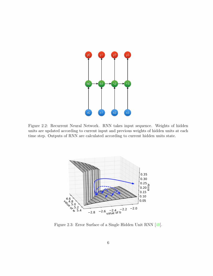
Figure 2.2: Recurrent Neural Network. RNN takes input sequence. Weights of hiddenunits are updated according to current input and previous weights of hidden units at eachtime step. Outputs of RNN are calculated according to current hidden units state.
Figure 2.3: Error Surface of a Single Hidden Unit RNN [41].
6
2.1.3 Recursive Neural Network
Recursive neural networks (RNNs) have been applied to multiple NLP tasks, such assentence classification [47].
Figure 2.4: Recursive Neural Network.
Figure 2.4 shows a simple recursive neural network. Each node takes two children asinputs. h = f(Wx + b) and y = UTh. For example, for the green node, the parent of
x0 and x1, h01 = f(W
✓x0
x1
◆+ b), and for the purple node, the parent of h01 and x2,
h012 = f(W
✓h01
x2
◆+ b). In CNNs, weights are shared within the same filter, while in
RNNs, weights are shared across di↵erent layers. Recursive neural networks have di↵erentcomposition functions: Matrix–Vector RNNs, Recursive Neural Tensor Networks, TreeLSTM, etc.
Recursive neural networks require parsers to get the semantic structures of the sen-tences. Recurrent neural networks are good at dealing with learning time–sequential fea-tures. Convolutional neural networks have good performances in classification and are usedas models for the task described in this thesis.
7
2.2 Motivation and History
Convolutional Neural Networks are inspired by a cat’s visual cortex. Visual cortex containsa complex arrangement of cells. These cells are responsible for detecting small sub–fieldsof the visual field, called receptive fields. The sub–fields are tiled to cover the whole visualfield. These cells act as local filters over the input space and are well–suited to exploit thestrong spatially local correlation present in natural images.
Neocognitron was introduced by Fukushima in 1980 [18] and improved in 1998 byLeCun, Bottou, Bengio, and Ha↵ner [30]. They proposed the famous LeNet–5 — a con-volutional neural network. Then it was generalized by Behnke [6], and pre-digested bySimard and his collaborators in 2003 [45]. Convolutional neural networks perform well onproblems such as recognizing handwritten numbers, but the computational power at thattime limited their ability to solve more complex problems until the rise of e�cient GPUcomputing.
2.3 Basic Assumption
The convolutional layer is based on the assumption that features are learned regardless oftheir absolute positions. This is reasonable in many cases, for example in image learning,if detecting a horizontal edge is important at some location in the image, it should also beuseful at other locations.
Convolutional layers focus on learning local features. In natural language processing,if in the sentence “give me an example of thank you letter” example of has been learnedas a feature, then it should also be recognized in sentence “what is an example of scientifichypothesis”. But example of may not have any relation with thank you letter or scientifichypothesis. For example in audio recognition, features of time spans of audio clips arelearned instead of that of the whole input audio.
2.4 Review of Discrete Convolution Definition
Recall the definition of convolution for a 1D signal [12]. The discrete convolution of f andg is given by:
o[n] = f [n] ⇤ g[n] =1X
u=�1f [u]g[n� u] =
1X
u=�1f [n� u]g[u]. (2.1)
8
This can be extended to 2D as follows:
o[m,n] = f [m,n] ⇤ g[m,n] =1X
u=�1
1X
v=�1f [u, v]g[m� u, n� v] (2.2)
2.5 Volumes of Neurons
The neurons in convolutional neural networks are arranged in three dimensions: depth,width, and height.
If the network is for image classification, images are in size of 3⇥ 32⇥ 32 (three colourchannels, 32 wide, 32 high). The size of input layer is 3⇥ 32⇥ 32. The size of hidden layeris 12⇥ 16⇥ 16 in which 12 is the number of feature maps and 16 is the width and heightof a feature map. The size of output layer is 10⇥ 1⇥ 1 where 10 is the number of classesto be learned.
If the network is for sentence classification, a sentence has 34 words and each word isrepresented by 300 dimensional vector. The size of input layer is 1⇥ 34⇥ 300. The size ofhidden layer might be 256⇥ 17⇥ 1 where 256 is the number of feature maps. The outputlayer has 46⇥ 1⇥ 1 dimensions for 46 class classification.
2.6 Architecture
Three types of layers build up a convolutional neural network: Convolutional Layer, PoolingLayer, and Fully Connected Layer.
2.6.1 Convolutional Layer
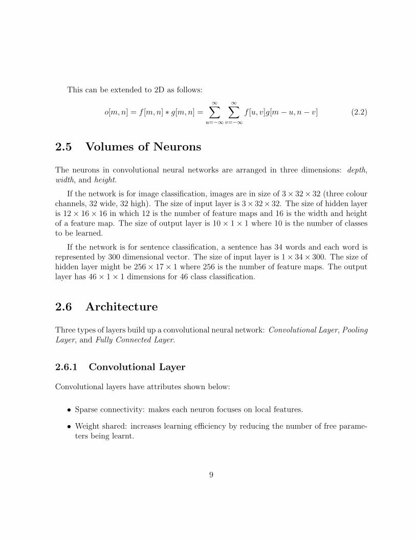
Convolutional layers have attributes shown below:
• Sparse connectivity: makes each neuron focuses on local features.
• Weight shared: increases learning e�ciency by reducing the number of free parame-ters being learnt.
9
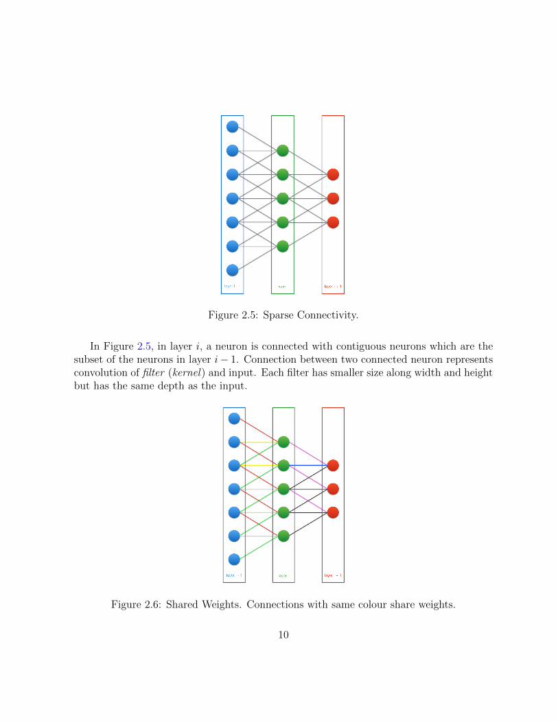
Figure 2.5: Sparse Connectivity.
In Figure 2.5, in layer i, a neuron is connected with contiguous neurons which are thesubset of the neurons in layer i� 1. Connection between two connected neuron representsconvolution of filter (kernel) and input. Each filter has smaller size along width and heightbut has the same depth as the input.
Figure 2.6: Shared Weights. Connections with same colour share weights.
10
Each filter learns a feature map. In the forward pass, when applying convolutionalcomputing, each filter is slid across the width and height and the dot product is computedbetween the entries of filter and the corresponding inputs. In Figure 2.6, weights of thesame colour are shared. In the back propagation process, calculating the gradient of ashared weight is to sum up the gradients of the parameters being shared.
A convolutional layer always has a set of filters. Feature maps learned by di↵erentfilters are stacked along depth dimension.
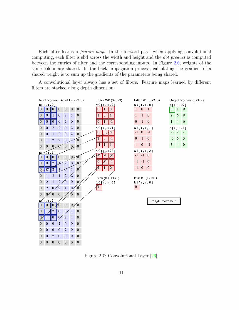
Figure 2.7: Convolutional Layer [26].
11
In Figure 2.7, input has size of di
⇥ wi
⇥ hi
= 3 ⇥ 5 ⇥ 5. Input is padded with 0s ofwidth w
p
= 1 and height hp
= 1. The depth of output (or the number of feature maps tobe learned) d
o
is 2. The size of filter is do
⇥ df
⇥ wf
⇥ hf
= 2 ⇥ 3 ⇥ 3 ⇥ 3. The strideswhen filter is slid along width w
s
and height hs
are both 1. The feature map hk
, which islearned by the filter k, is determined by the weights W
k
and bias bk
as follows:
hk
= f(Wk
⇤ x+ bk
) (2.3)
, where f is an activation function which will be introduced in Subsection 2.6.5. Thevolume of output should be:
do
⇥ (w
i
� wf
+ 2wp
ws
+ 1)⇥ (hi
� hf
+ 2hp
hs
+ 1) (2.4)
The number of parameters to be learned should be:
(wf
· hf
· df
+ 1) · od
(2.5)
i.e., The output has size of 2⇥ 3⇥ 3. The number of parameters to be learned is (3⇥ 3⇥3 + 1)⇥ 2 = 56.
In regular neural networks, every neuron is fully connected with all neurons in theprevious layer. If the sizes of input and output are the same, the number of parameters ofa fully connected neural network becomes (w
i
·hi
·di
+1)·wo
·ho
·do
= (7⇥7⇥3+1)⇥3⇥3⇥2 =2664. The number of parameters in a convolutional neural network is positively correlatedwith the size of the filter, while that in a regular neural network is positively correlatedwith the size of the input and the output. But the size of filter is much smaller than thatof input and output. The number of parameters in regular neural network is very largeas every layer is fully connected with neighbour layers, which sometimes makes learningprocess overfitting.
2.6.2 Pooling Layer
To describe a large matrix, one natural approach to down sample is to aggregate statistics.Common methods include computing themean value, max value and L2–norm of particularsize. By doing this, the problem of overfitting is addressed to a certain degree.
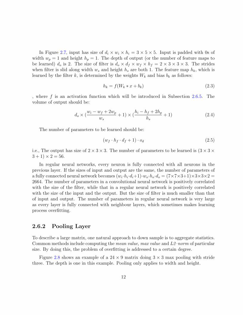
Figure 2.8 shows an example of a 24 ⇥ 9 matrix doing 3 ⇥ 3 max pooling with stridethree. The depth is one in this example. Pooling only applies to width and height.
12
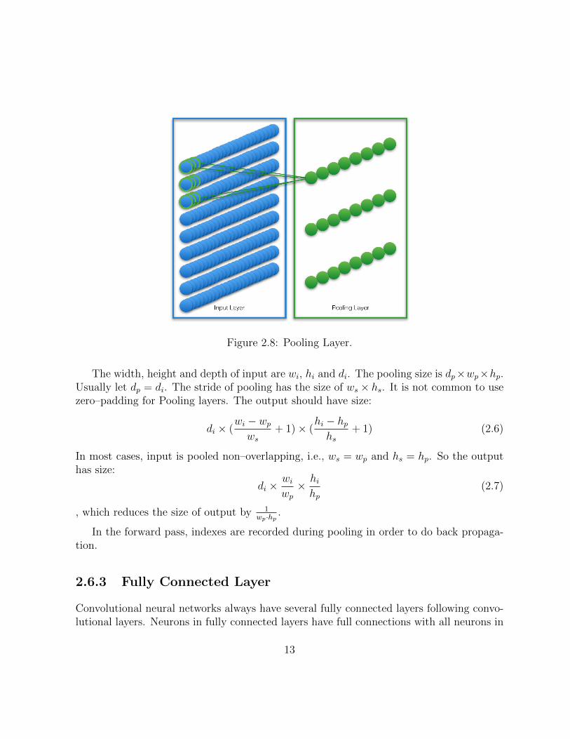
Figure 2.8: Pooling Layer.
The width, height and depth of input are wi
, hi
and di
. The pooling size is dp
⇥wp
⇥hp
.Usually let d
p
= di
. The stride of pooling has the size of ws
⇥ hs
. It is not common to usezero–padding for Pooling layers. The output should have size:
di
⇥ (w
i
� wp
ws
+ 1)⇥ (hi
� hp
hs
+ 1) (2.6)
In most cases, input is pooled non–overlapping, i.e., ws
= wp
and hs
= hp
. So the outputhas size:
di
⇥ wi
wp
⇥ hi
hp
(2.7)
, which reduces the size of output by 1wp·hp
.
In the forward pass, indexes are recorded during pooling in order to do back propaga-tion.
2.6.3 Fully Connected Layer
Convolutional neural networks always have several fully connected layers following convo-lutional layers. Neurons in fully connected layers have full connections with all neurons in
13
the previous layer. The structure of a fully connected layer is same as that of layer in aregular neural network.
2.6.4 Dropout
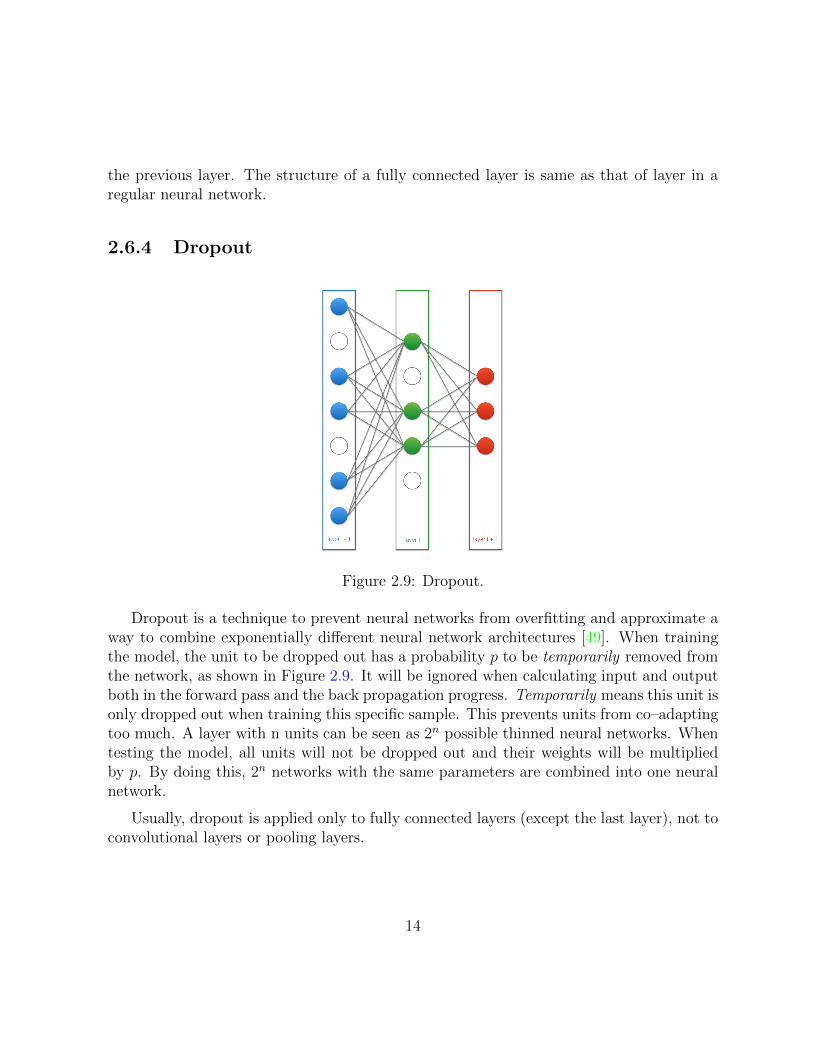
Figure 2.9: Dropout.
Dropout is a technique to prevent neural networks from overfitting and approximate away to combine exponentially di↵erent neural network architectures [49]. When trainingthe model, the unit to be dropped out has a probability p to be temporarily removed fromthe network, as shown in Figure 2.9. It will be ignored when calculating input and outputboth in the forward pass and the back propagation progress. Temporarily means this unit isonly dropped out when training this specific sample. This prevents units from co–adaptingtoo much. A layer with n units can be seen as 2n possible thinned neural networks. Whentesting the model, all units will not be dropped out and their weights will be multipliedby p. By doing this, 2n networks with the same parameters are combined into one neuralnetwork.
Usually, dropout is applied only to fully connected layers (except the last layer), not toconvolutional layers or pooling layers.
14
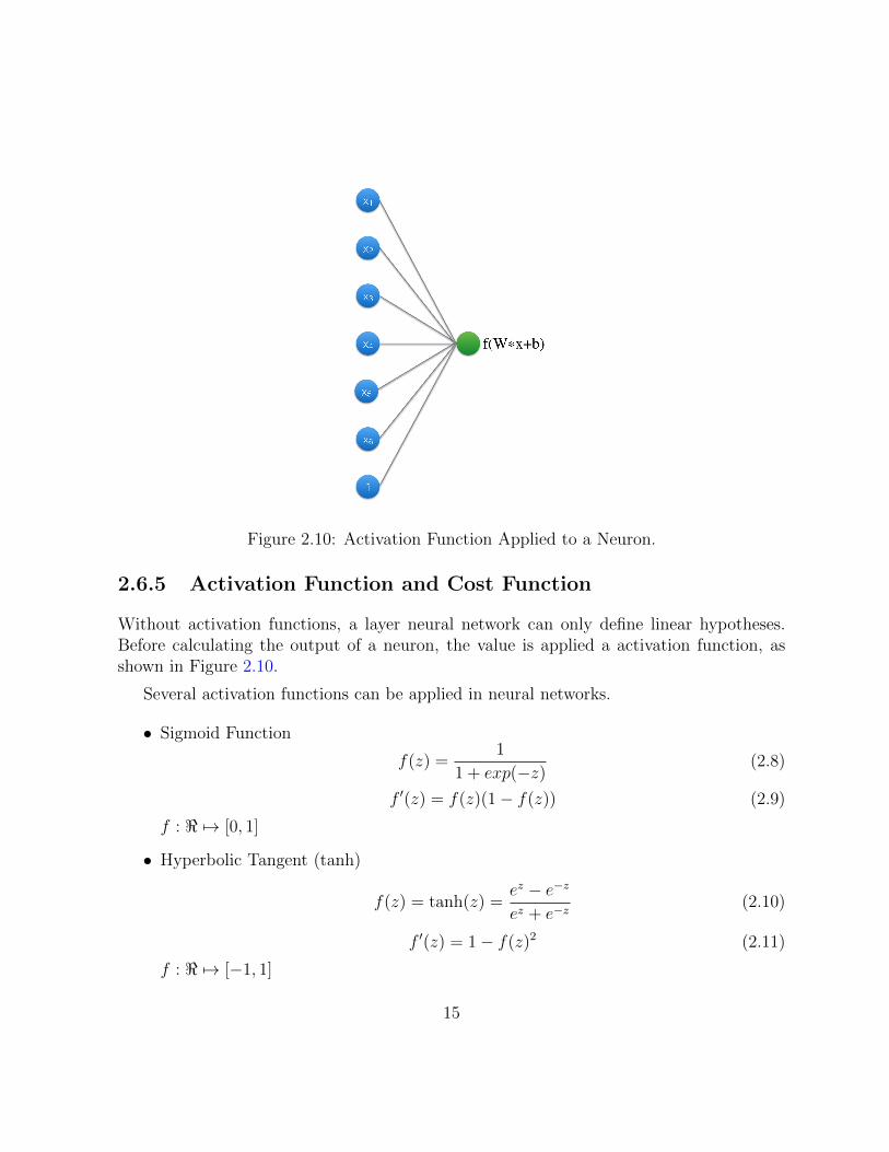
Figure 2.10: Activation Function Applied to a Neuron.
2.6.5 Activation Function and Cost Function
Without activation functions, a layer neural network can only define linear hypotheses.Before calculating the output of a neuron, the value is applied a activation function, asshown in Figure 2.10.
Several activation functions can be applied in neural networks.
• Sigmoid Function
f(z) =1
1 + exp(�z)(2.8)
f 0(z) = f(z)(1� f(z)) (2.9)
f : < 7! [0, 1]
• Hyperbolic Tangent (tanh)
f(z) = tanh(z) =ez � e�z
ez + e�z
(2.10)
f 0(z) = 1� f(z)2 (2.11)
f : < 7! [�1, 1]
15
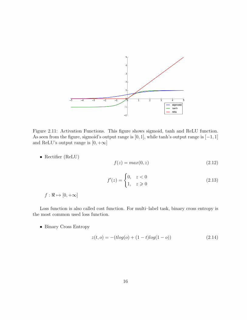
Figure 2.11: Activation Functions. This figure shows sigmoid, tanh and ReLU function.As seen from the figure, sigmoid’s output range is [0, 1], while tanh’s output range is [�1, 1]and ReLU’s output range is [0,+1]
• Rectifier (ReLU)f(z) = max(0, z) (2.12)
f 0(z) =
(0, z < 0
1, z > 0(2.13)
f : < 7! [0,+1]
Loss function is also called cost function. For multi–label task, binary cross entropy isthe most common used loss function.
• Binary Cross Entropy
z(t, o) = �(tlog(o) + (1� t)log(1� o)) (2.14)
16
2.6.6 Common CNN Architectures
Most common convolutional neural networks follow the pattern below [26]:
Input
! [(Convolutional ! Activation)⇤ ! Pooling?]⇤
! (FC ! Dropout? ! Activation)⇤
! Output
(2.15)
, where “*” indicates that this layer might be repeated multiple times and “?” stands foroptional occurring. Input layer is followed by multiple convolutional and pooling layers,then is followed by several fully connected layers with dropout.
17
Chapter 3
Related Work
Convolutional neural networks have been widely used in POS tagging [43], chunking, NER,semantic role labeling [10], searching queries and Web documents [44], sentence classifica-tion [13] [27], semantic modelling [25], relation classification [14], and other NLP tasks.
3.1 Single–Convolutional–Layer CNNs
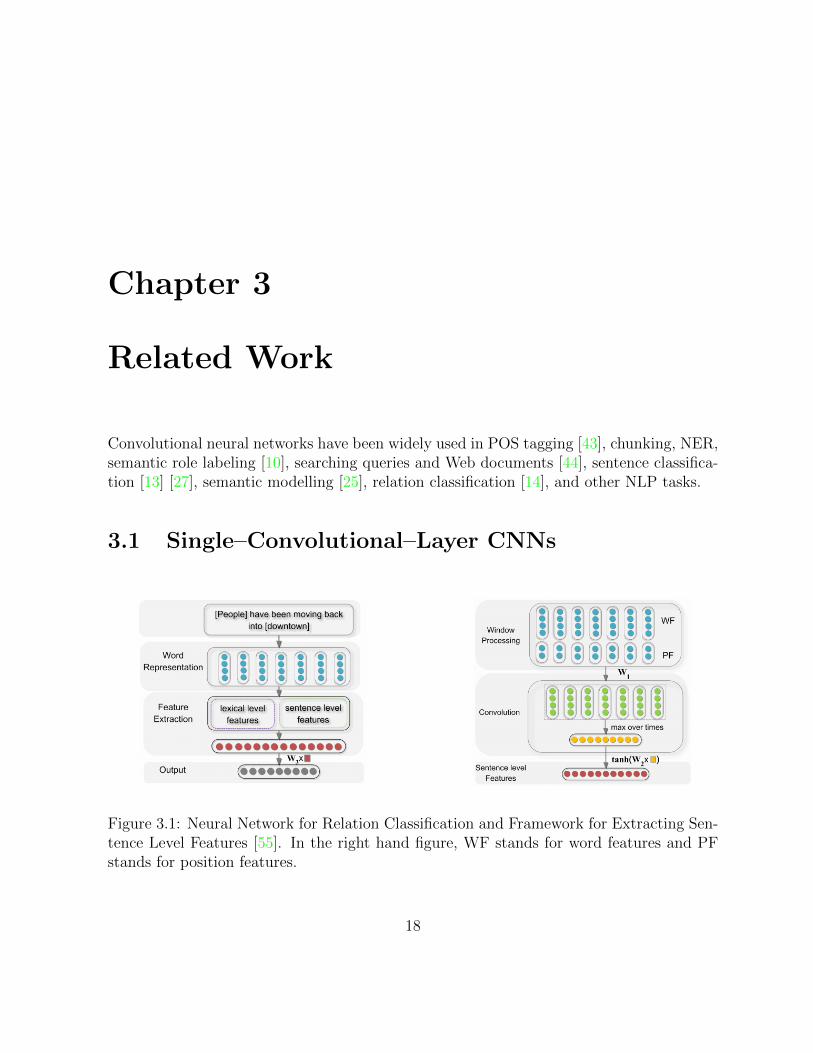
Figure 3.1: Neural Network for Relation Classification and Framework for Extracting Sen-tence Level Features [55]. In the right hand figure, WF stands for word features and PFstands for position features.
18
Zeng et al. [55] exploit a neural network to classify questions. Lexical level featuresare extracted from word embeddings. Sentence level features are learned by a one layerconvolutional neural network. Then both lexical and sentence level features are fed into aneural network to predict the relationship of two given nouns in a sentence, as shown inFigure 3.1. This model is experimented on the SemEval–2010 Task 8 dataset (a questionset with 10 labels [20]).
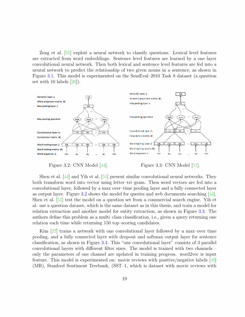
Figure 3.2: CNN Model [44]. Figure 3.3: CNN Model [51].
Shen et al. [44] and Yih et al. [51] present similar convolutional neural networks. Theyboth transform word into vector using letter–tri–gram. Then word vectors are fed into aconvolutional layer, followed by a max over–time pooling layer and a fully connected layeras output layer. Figure 3.2 shows the model for queries and web documents searching [44].Shen et al. [51] test the model on a question set from a commercial search engine. Yih etal. use a question dataset, which is the same dataset as in this thesis, and train a model forrelation extraction and another model for entity extraction, as shown in Figure 3.3. Theauthors define this problem as a multi–class classification, i.e., given a query returning onerelation each time while returning 150 top–scoring candidates.
Kim [27] trains a network with one convolutional layer followed by a max–over timepooling, and a fully connected layer with dropout and softmax output layer for sentenceclassification, as shown in Figure 3.4. This “one convolutional layer” consists of 3 parallelconvolutional layers with di↵erent filter sizes. The model is trained with two channels –only the parameters of one channel are updated in training progress. word2vec is inputfeature. This model is experimented on: movie reviews with positive/negative labels [40](MR), Stanford Sentiment Treebank, (SST–1, which is dataset with movie reviews with
19

Figure 3.4: CNN Model for Several Sentence Classification Tasks [27].
very positive, positive, neutral, negative, very negative label [48]), same dataset as SST–1but only positive/negative labels, sentences with subjective/objective labels [39] (Subj),Text REtrieval Conference question dataset with 6 labels [32] (TREC), customer reviewswith positive/negative labels [23] (CR), opinion dataset with positive/negative labels [52](MPQA).
3.2 Multi–Convolutional–Layer CNNs
Figure 3.5: ARC–II Model [22].
Hu et al. [22] propose a convolutional neural network model for matching sentences. Theauthors apply a 1 dimension convolution followed by 1 dimension max pooling, multiple 2
20

dimension convolutions and pooling layers, and multiple fully connected layers, as shownin Figure 3.5. It takes embedding of words in the sentences aligned as input and outputsmatching degree. The approach is tested on sentence completion [31], matching a responseto Weibo, and MSRP dataset [42]
Figure 3.6: DCNN Model for Modeling Sentence [25].
Kalchbrenner et al. [25] design a Dynamic k–Max Pooling Convolutional Neural Net-work (DCNN) for sentence modelling. The authors apply several wide one–dimensionalconvolution layer followed by feature maps folding operation and k–max pooling layer, anda fully connected layer as output, which is shown as Figure 3.6. K–max pooling is to chosek highest values among inputs and keep their original orders. This model is tested onSST–1, SST–2, 6–type question categorization in the TREC dataset, and Twitter senti-ment prediction task (tweets with positive/negative labels). Compared with Kim’s model,
21
DCNN performs better on SST–1 and TREC, while worse on SST–2.
CNNs with only one convolutional layer have good performance on di↵erent tasks.Kim’s design [27] consists of parallel convolutional layers which is di↵erent from others’.Some other authors propose deeper CNNs. This thesis proposes a single–layer CNN andtwo multi–layer CNNs and compares their performance on di↵erent datasets.
22
Chapter 4
Dataset and Environment
4.1 Dataset
This thesis focuses on classifying single–relation questions. Example questions of thistype include: “What is the birthday of Barack Obama?”, “Where does a giant swallowtailbutterfly live?”. Single–relation questions are the most common type of questions observedin various community QA sites [16]. In a single–relation question, relation and entity aretwo elements to be understood. After the relation and the entity are extracted, the answercan be generated from knowledge base (KB) such as Freebase [2], DBpedia [1], etc.
4.1.1 Data Format
In this thesis, we download the dataset from knowitall.cs.washington.edu/paralex/ [16].These questions are crawled from WikiAnswer. Typos and grammar errors are very com-mon in the dataset. “labeled.txt” contains 608,650 examples. Each example is in theform of (question, query1, query2, . . .), for instance, “what be the di↵erence btw isolationtransformer and step up and step down transformer ? 2 1 755225 1605804 2 1 7758542464747 2 1 887236 1605804 2 1 890251 1605804 2 0 1503166”. Each query is encoded inthe form 2#ORDER#REL#ENT . #REL represents index of relation constants in thequery which can be looked up in “vocab.txt”, such as 755225 stands for be–function–of.r.Each question might have several relations. All question–queries list tuples are processedto generate question–relations list tuples in the form of (question,#REL1,#REL2, . . .).The example mentioned above becomes “what be the di↵erence btw isolation transformerand step up and step down transformer ? 755225 775854 887236 890251 1503166”.
23

4.1.2 Answerable Queries Coverage
Figure 4.1: The Curve of Coverage of Queries Answerable and Number of Relation.
Figure 4.1 shows the relation between the coverage of answerable queries and the num-ber of relations. This curve increases steeply before coverage reaches 80% but grows slowlylater. 21 relations cover more than 20% of the queries. But it requires about 16,000 addi-tional relations to increase the coverage from 80% to 100%. It makes sense that most ofthe problems people concern on WikiAnswer are only a small subset of knowledge.
4.2 Tool and Environment
4.2.1 word2vec
Word2vec is a continuous distributed representation of words [33] [35] [36]. A 300 dimen-sional vectors trained on part of Google News dataset which contains 3 million words andphrases are used in this experiment.
24
4.2.2 NER
NER labels named entities. Stanford NER has three models: a four–class model trainedfor CoNLL, a seven–class model trained for MUC and a three–class model trained forboth [17] [19]. Models support both capitalization sensitive and ignored classifiers.
4.2.3 CUDA
In order to run experiments on GPU, CUDA driver and CUDA Toolkit are needed forNvidia’s GPU–programming toolchain. CUDA Toolkit is downloaded from developer.nvidia.com,which contains an nvcc program – a compiler for GPU code.
4.2.4 Python Libraries
• Theano is a Python library that defines, optimizes, and evaluates mathematical ex-pressions involving multi–dimensional arrays e�ciently and has transparent use ofGPU [5] [7] [28].
• Keras is a Theano–based deep learning Python library [3]. Keras is used as libraryto build CNNs.
• scikit–learn is a Python library for machine learning [4]. scikit–learn is for buildinga support vector classifier.
4.2.5 Spelling Corrector
Spelling Corrector is a tool to correct typos [38]. It is used to correct spelling errors indataset with pre–trained 3 million words and phrases (GoogleNews–vectors–negative3000)as dictionary. As questions of are crawled from WikiAnswer, dataset contains many typosand grammar error. Spelling corrector is helpful to remove noises in dataset.
4.2.6 Experiment Environment
All the experiments are tested with the computer with configuration described as follows:
• OS system: Ubuntu 14.04LTS
25
• Processer: Intel Core i7–4790K CPU @ 4.00GHz ⇥ 8
• Memory: 16GB 1333 MHz DDR3
• GPU: NVIDIA GeForce GTX TITIAN X
• JDK: 1.8.0 45
• Python: 2.7.6
• NumPy: 1.9.2
• SciPy: 0.15.1
• Theano: 0.7.0
• Keras: 0.1.1
26

Chapter 5
Main Results
5.1 Methodologies
5.1.1 Data Processing
Raw Data
Dataset Index #Sentences #Classes Min #Sentences per Class1 138280 22 80002 202002 55 40003 261681 120 2000
Table 5.1: Three Datasets. Each subset is chosen from the whole dataset according tominimum sentences per class. For example, for subset 1, only classes which have morethan 8000 sample sentences will be chosen.
Three datasets were used for experiments. Table 5.1 shows the number of sentences,classes and the minimum number of sentences per class of each dataset. Each dataset splits110 for test1.
1Actually, k–fold cross validation is better than conventional validation. The former more properly
estimates model prediction performance. But training a model takes up to 9000s per epoch. 10–fold cross
validation needs 10 times training and testing processes. As the size of dataset is very large, and results of
di↵erent choice of subset to be the test set do not di↵er with each other a lot. So we still use
910 as train
set and
110 as test set.
27
Then sentences were corrected spelling errors using GoogleNews–vectors–negative300 asa dictionary. All name entities in sentences were replaced by “LOC”, “PER” and “ORG”with Stanford NER [36] 3 class model trained for both CoNLL and MUC in capitalizationignored mode.
Sentence Space
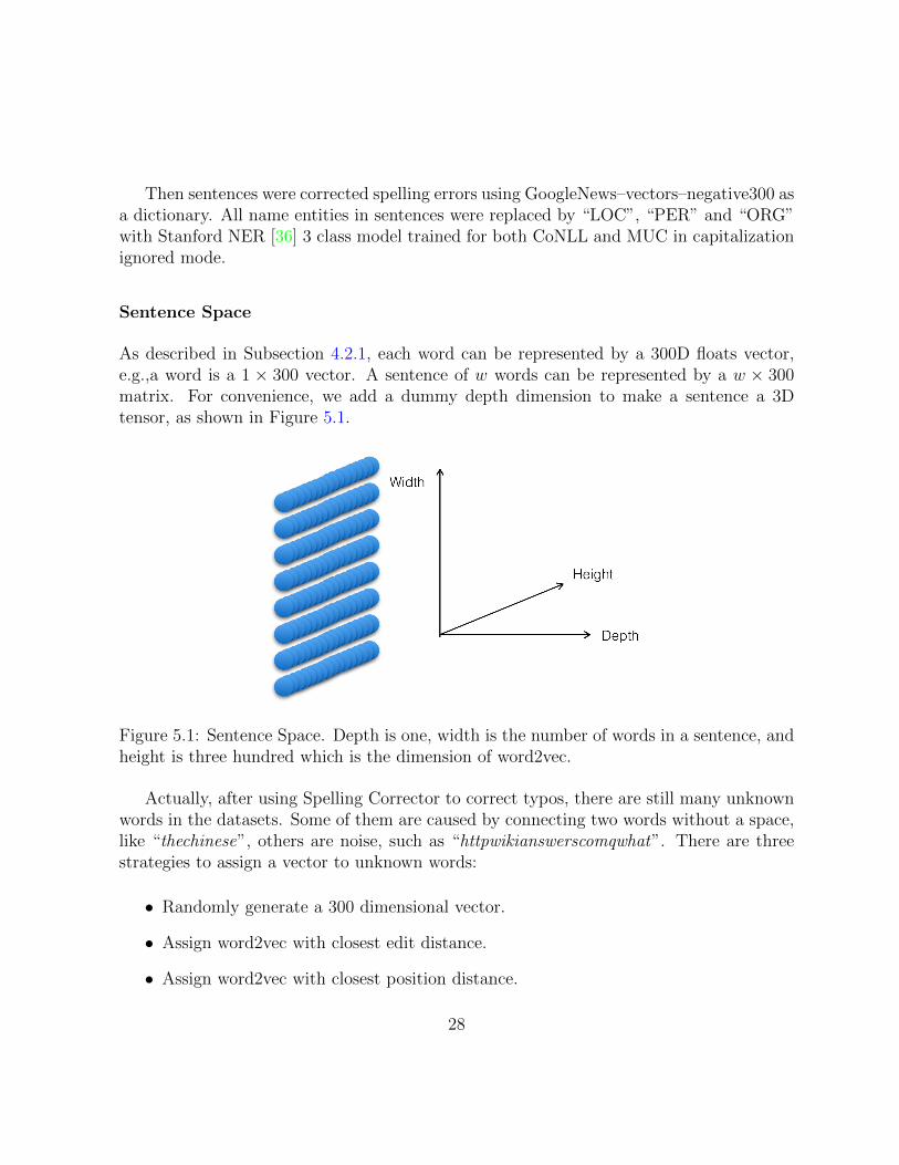
As described in Subsection 4.2.1, each word can be represented by a 300D floats vector,e.g.,a word is a 1 ⇥ 300 vector. A sentence of w words can be represented by a w ⇥ 300matrix. For convenience, we add a dummy depth dimension to make a sentence a 3Dtensor, as shown in Figure 5.1.
Figure 5.1: Sentence Space. Depth is one, width is the number of words in a sentence, andheight is three hundred which is the dimension of word2vec.
Actually, after using Spelling Corrector to correct typos, there are still many unknownwords in the datasets. Some of them are caused by connecting two words without a space,like “thechinese”, others are noise, such as “httpwikianswerscomqwhat”. There are threestrategies to assign a vector to unknown words:
• Randomly generate a 300 dimensional vector.
• Assign word2vec with closest edit distance.
• Assign word2vec with closest position distance.
28
Position distance of two words is defined as Manhattan distance between their letter–bigrams vectors. Given a word, after adding word boundary symbols, we divide it intoa sequence of letter–bigrams. For example, ‘word ’ is divided into ‘ˆw ’, ‘wo’,‘or ’,‘rd ’ and‘d$’, v(word) = (0, . . . , 1, . . . , 1, . . . , 0) where 1s are indexes of ‘ˆw ’, ‘wo’,‘or ’,‘rd ’ and ‘d$’in the bigrams dictionary.
Since each sentence in the dataset has at most 18 words, it can be represented by a1 ⇥ 18 ⇥ 300 tensor. Zero paddings are added at the end of a sentence if it has less than18 words.
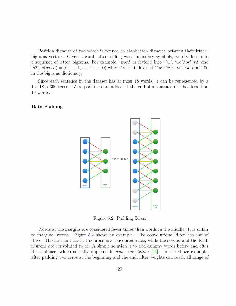
Data Padding
Figure 5.2: Padding Zeros.
Words at the margins are considered fewer times than words in the middle. It is unfairto marginal words. Figure 5.2 shows an example. The convolutional filter has size ofthree. The first and the last neurons are convoluted once, while the second and the forthneurons are convoluted twice. A simple solution is to add dummy words before and afterthe sentence, which actually implements wide convolution [25]. In the above example,after padding two zeros at the beginning and the end, filter weights can reach all range of
29
input and each input is convoluted 3 times. The feature map of the narrow convolution is asubsequence of the feature map of the wide convolution. The input of CNN is a 1⇥26⇥300tensor.
5.1.2 Multi–Label Classification
Sentence Relations
The old name of Bangkok?
bangkok.rbe–in–in.r
be–last–name–of.rbe–o�cial–name–of.rbe–other–name–for.r
be–real–name–of.rbe–traditional–name–for.r
use–to–be–call.r
What be SSID broadcasting?
be–function–of.rbe–know–as.r
be–purpose–of.rbe–requirement–for.r
function.rhave–function–of.rhave–purpose–of.r
What be the primary duty ofjudical(typo: judicial) branch?
be–judicial–branch–of.rbe–primary–of.r
be–primary–responsibility–of.rbe–primary–role–of.r
be–role–of.rhave–role–of.r
Table 5.2: Multi–Label Task for Relation Classification Example.
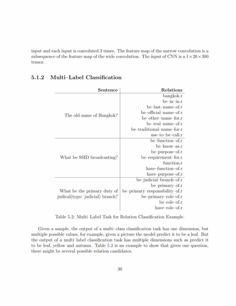
Given a sample, the output of a multi–class classification task has one dimension, butmultiple possible values, for example, given a picture the model predict it to be a leaf. Butthe output of a multi–label classification task has multiple dimensions such as predict itto be leaf, yellow and autumn. Table 5.2 is an example to show that given one question,there might be several possible relation candidates.
30
Label Space
In supervised learning, training set has a set of examples in the form of (x, y) such that xis the feature and y is the label. X is the input space while Y is the output space. Thenumber of label dimensions of each sample is not constant. Sample s1 might have labely = (y1, y2, y3) while sample s2 might have label y = (y1, y4). But the dimensions of outputspace Y is limited. First of all, if the dimensions of Y is N , these labels can be indexedfrom 0 to N � 1. Then 8y 2 Y can be represented by an N dimension binary vector like(0, . . . , 0, 1, 0, . . . , 0, 1, 0, . . . , 0) where indexes (i1, . . . , ik) of 1s indicate y = (i1, . . . , ik).
5.1.3 Models
CNN Models Deep CNN Parallel CNN
1st Conv Layer (27, 1, 3, 1)
(512, 1, 2, 300)(512, 1, 3, 300)(512, 1, 4, 300)(512, 1, 5, 300)
2nd Conv Layer (2048, 27, 3, 300) -
Pooling Size (22, 1)
(25, 1)(24, 1)(23, 1)(22, 1)
1st Fully Connected Layer (2048, 256) (2048, 256)2nd Fully Connected Layer (256, #Classes) (256, #Classes)
Table 5.3: Parameters for CNNs.
Deep CNN
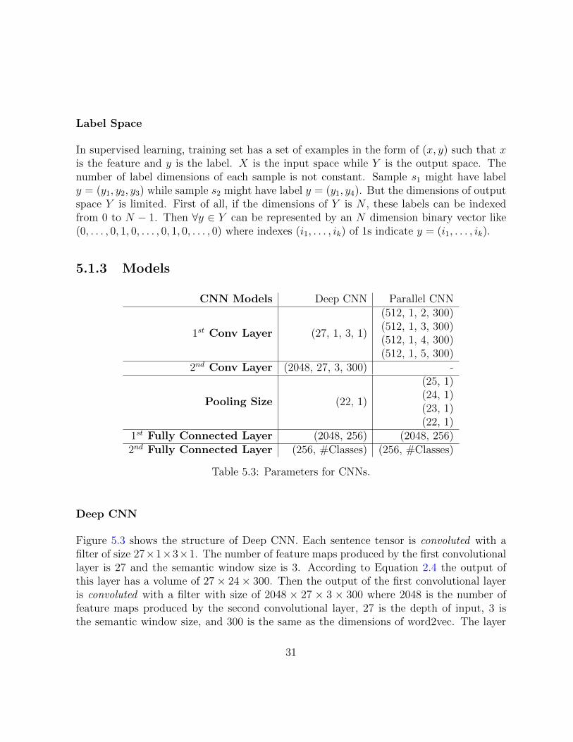
Figure 5.3 shows the structure of Deep CNN. Each sentence tensor is convoluted with afilter of size 27⇥1⇥3⇥1. The number of feature maps produced by the first convolutionallayer is 27 and the semantic window size is 3. According to Equation 2.4 the output ofthis layer has a volume of 27⇥ 24⇥ 300. Then the output of the first convolutional layeris convoluted with a filter with size of 2048 ⇥ 27 ⇥ 3 ⇥ 300 where 2048 is the number offeature maps produced by the second convolutional layer, 27 is the depth of input, 3 isthe semantic window size, and 300 is the same as the dimensions of word2vec. The layer
31
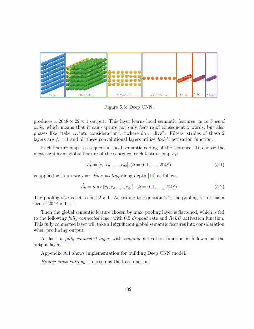
Figure 5.3: Deep CNN.
produces a 2048 ⇥ 22 ⇥ 1 output. This layer learns local semantic features up to 5 wordwide, which means that it can capture not only feature of consequent 5 words, but alsophases like “take . . . into consideration”, “where do . . . live”. Filters’ strides of these 2layers are f
s
= 1 and all these convolutional layers utilize ReLU activation function.
Each feature map is a sequential local semantic coding of the sentence. To choose themost significant global feature of the sentence, each feature map h
k
:
~hk
= [c1, c2, . . . , c22], (k = 0, 1, . . . , 2048) (5.1)
is applied with a max–over–time pooling along depth [10] as follows:
hk
= max{c1, c2, . . . , c22}, (k = 0, 1, . . . , 2048) (5.2)
The pooling size is set to be 22 ⇥ 1. According to Equation 2.7, the pooling result has asize of 2048⇥ 1⇥ 1.
Then the global semantic feature chosen by max–pooling layer is flattened, which is fedto the following fully connected layer with 0.5 dropout rate and ReLU activation function.This fully connected layer will take all significant global semantic features into considerationwhen producing output.
At last, a fully connected layer with sigmoid activation function is followed as theoutput layer.
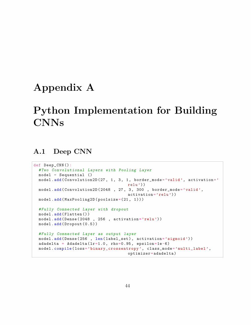
Appendix A.1 shows implementation for building Deep CNN model.
Binary cross entropy is chosen as the loss function.
32
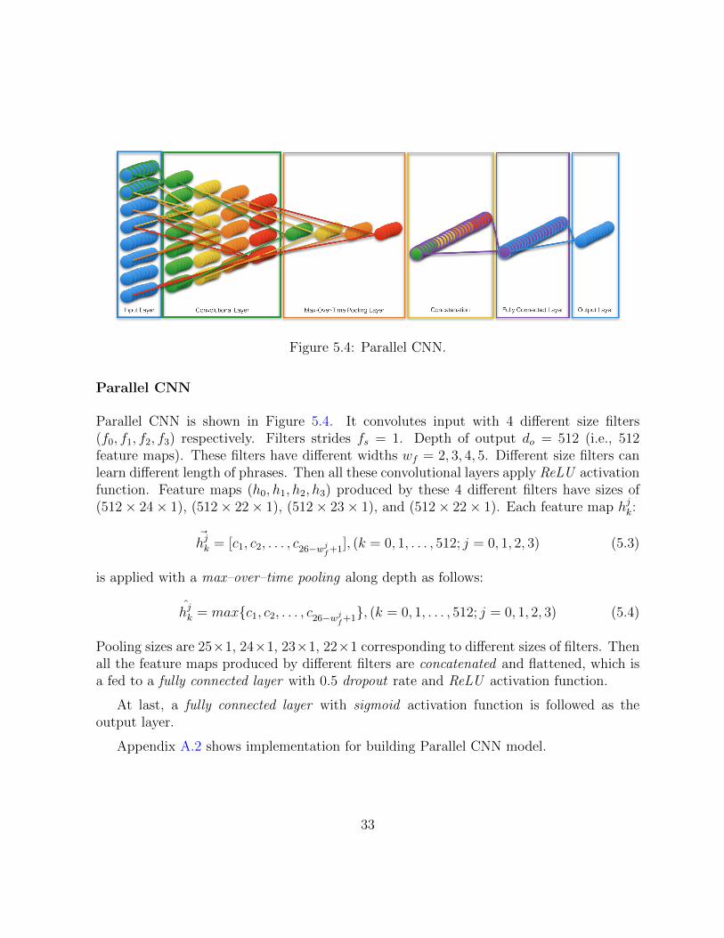
Figure 5.4: Parallel CNN.
Parallel CNN
Parallel CNN is shown in Figure 5.4. It convolutes input with 4 di↵erent size filters(f0, f1, f2, f3) respectively. Filters strides f
s
= 1. Depth of output do
= 512 (i.e., 512feature maps). These filters have di↵erent widths w
f
= 2, 3, 4, 5. Di↵erent size filters canlearn di↵erent length of phrases. Then all these convolutional layers apply ReLU activationfunction. Feature maps (h0, h1, h2, h3) produced by these 4 di↵erent filters have sizes of(512⇥ 24⇥ 1), (512⇥ 22⇥ 1), (512⇥ 23⇥ 1), and (512⇥ 22⇥ 1). Each feature map hj
k
:
~hj
k
= [c1, c2, . . . , c26�w
jf+1], (k = 0, 1, . . . , 512; j = 0, 1, 2, 3) (5.3)
is applied with a max–over–time pooling along depth as follows:
hj
k
= max{c1, c2, . . . , c26�w
jf+1}, (k = 0, 1, . . . , 512; j = 0, 1, 2, 3) (5.4)
Pooling sizes are 25⇥1, 24⇥1, 23⇥1, 22⇥1 corresponding to di↵erent sizes of filters. Thenall the feature maps produced by di↵erent filters are concatenated and flattened, which isa fed to a fully connected layer with 0.5 dropout rate and ReLU activation function.
At last, a fully connected layer with sigmoid activation function is followed as theoutput layer.
Appendix A.2 shows implementation for building Parallel CNN model.
33
ADADELTA
ADADELTA is a kind of gradient descent learning rate method [54]. It takes each di-mension’s first order information into consideration when updating learning rate. Thisapproach has several advantages:
• Dynamic learning rate per dimension.
• Small amount of computation each iteration.
• Hyperparameters chosen do not a↵ect result significantly.
In the experiment, ✏ = 1e�6, ⇢ = 0.95, and ⌘ = 1 are set to be hyperparameters ofADADELTA, where ✏ is a constant controlling the decay rate and ⌘ is a global learningrate shared by all dimensions.
5.1.4 Evaluation Metrics
As described in Section 5.1.2, each sample (query) might have several relation candidates.Label of each sample is converted into an N–dimensional sparse binary vector, where N isthe number of all possible relations.
When evaluating the result, precision, recall and F1 are chosen to be evaluation metrics.
Precision =TP
TP + FP(5.5)
Recall =TP
TP + FN(5.6)
F1 = 2 · Precision ·Recall
Precision+Recall(5.7)
, where T stands for true, F for false, P for positive and N for negative. For example,if the ground truth of a sentence s1 is (y1, y2, y3), and the predicted label is (y1, y4), thenPrecision = 1
2 and Recall = 13 . F1 score is their harmonic mean F1 =
25
There are three methods to calculate average statistic: micro–average, macro–averageand sample–average.
• Micro–average: calculate metrics by counting the total TP, FN and FP globally.
34
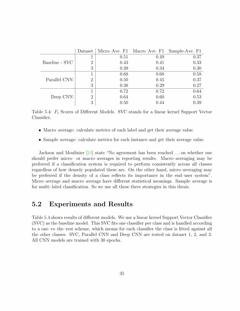
Dataset Micro–Ave. F1 Macro–Ave. F1 Sample-Ave. F1
Baseline - SVC1 0.51 0.49 0.372 0.43 0.41 0.333 0.39 0.34 0.30
Parallel CNN1 0.68 0.68 0.582 0.50 0.45 0.373 0.38 0.29 0.27
Deep CNN1 0.72 0.72 0.642 0.64 0.60 0.533 0.50 0.44 0.39
Table 5.4: F1 Scores of Di↵erent Models. SVC stands for a linear kernel Support VectorClassifier.
• Macro–average: calculate metrics of each label and get their average value.
• Sample–average: calculate metrics for each instance and get their average value.
Jackson and Moulinier [24] state “No agreement has been reached . . . on whether oneshould prefer micro– or macro–averages in reporting results. Macro–averaging may bepreferred if a classification system is required to perform consistently across all classesregardless of how densely populated these are. On the other hand, micro–averaging maybe preferred if the density of a class reflects its importance in the end–user system”.Micro–average and macro–average have di↵erent statistical meanings. Sample–average isfor multi–label classification. So we use all these three strategies in this thesis.
5.2 Experiments and Results
Table 5.4 shows results of di↵erent models. We use a linear kernel Support Vector Classifier(SVC) as the baseline model. This SVC fits one classifier per class and is handled accordingto a one–vs–the–rest scheme, which means for each classifier the class is fitted against allthe other classes. SVC, Parallel CNN and Deep CNN are tested on dataset 1, 2, and 3.All CNN models are trained with 30 epochs.
35
5.2.1 Baseline versus CNNs
Results show that Parallel CNN and Deep CNN perform remarkably well, giving competi-tive results against SVC, on dataset 1 and dataset 2, while Parallel CNN has similar resultson dataset 3 compared with SVC.
5.2.2 Parallel versus Deep CNN
Deep CNN has better performance than Parallel CNN on dataset 1, 2 and 3. Deep CNNhas two convolutional layers while Parallel CNN has four parallel convolutional layers.Although the number of feature maps learned by the second convolutional layer in DeepCNN (2048) is the same as that of the convolutional layer in Parallel CNN, and maximumlength of phrases learned by convolutional filters of both models are five, the multi–layerCNN is more powerful than the single–layer CNN.
We can either increase the number of convolutional layers or the number of neuronswithin each layer to improve the performance by sacrificing training time.
5.2.3 Further Observations
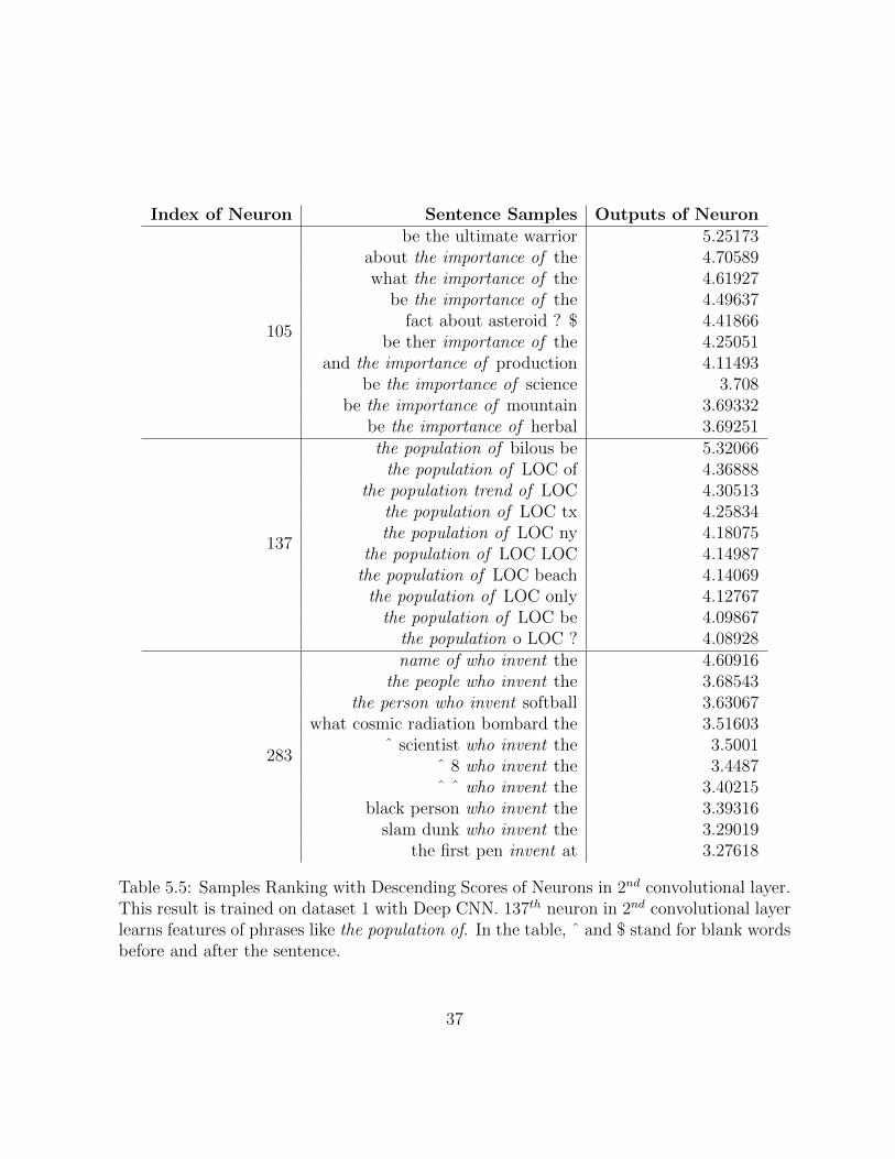
In Deep CNN, the first convolutional layer acts as masks of phrases, which masks “whichpredator eat leopard” into “which X eat X”. The second convolutional layer learns phrases.Table 5.5 shows samples recognized by the filters of the second convolutional layer. Eachfilter in the 2nd convolutional layer learns at least one phrase ideally. By stacking featuremaps learned by di↵erent filters, the convolutional layer can recognize large number ofphrases.
Figure 5.5 shows precision against recall at various threshold settings of each classon dataset 1. A high area under the PR curve (AUC) represents both high recall andhigh precision. AUCs range from 0.66 to 0.95. Average AUC is 0.70. Figure 5.6 showsTP against FP at various threshold settings each class on dataset 1. Receiver operatingcharacteristic (ROC) is another metric for evaluating the performance of a binary classifier.ROCs range from 0.90 to 0.99. Average ROC area is 0.97. Closer the curve is to upperleft corner, lower the false negative rate and false positive rate are.
Previous results show that the proposed CNNs have good performance on sentenceclassification. Convolution works well on learning local features (phrases) and max poolingcan choose the most significant global feature. As the dataset gets larger, a small CNN is
36
Index of Neuron Sentence Samples Outputs of Neuron
105
be the ultimate warrior 5.25173about the importance of the 4.70589what the importance of the 4.61927
be the importance of the 4.49637fact about asteroid ? $ 4.41866
be ther importance of the 4.25051and the importance of production 4.11493
be the importance of science 3.708be the importance of mountain 3.69332
be the importance of herbal 3.69251
137
the population of bilous be 5.32066the population of LOC of 4.36888
the population trend of LOC 4.30513the population of LOC tx 4.25834the population of LOC ny 4.18075
the population of LOC LOC 4.14987the population of LOC beach 4.14069the population of LOC only 4.12767the population of LOC be 4.09867
the population o LOC ? 4.08928
283
name of who invent the 4.60916the people who invent the 3.68543
the person who invent softball 3.63067what cosmic radiation bombard the 3.51603
ˆ scientist who invent the 3.5001ˆ 8 who invent the 3.4487ˆ ˆ who invent the 3.40215
black person who invent the 3.39316slam dunk who invent the 3.29019
the first pen invent at 3.27618
Table 5.5: Samples Ranking with Descending Scores of Neurons in 2nd convolutional layer.This result is trained on dataset 1 with Deep CNN. 137th neuron in 2nd convolutional layerlearns features of phrases like the population of. In the table, ˆ and $ stand for blank wordsbefore and after the sentence.
37
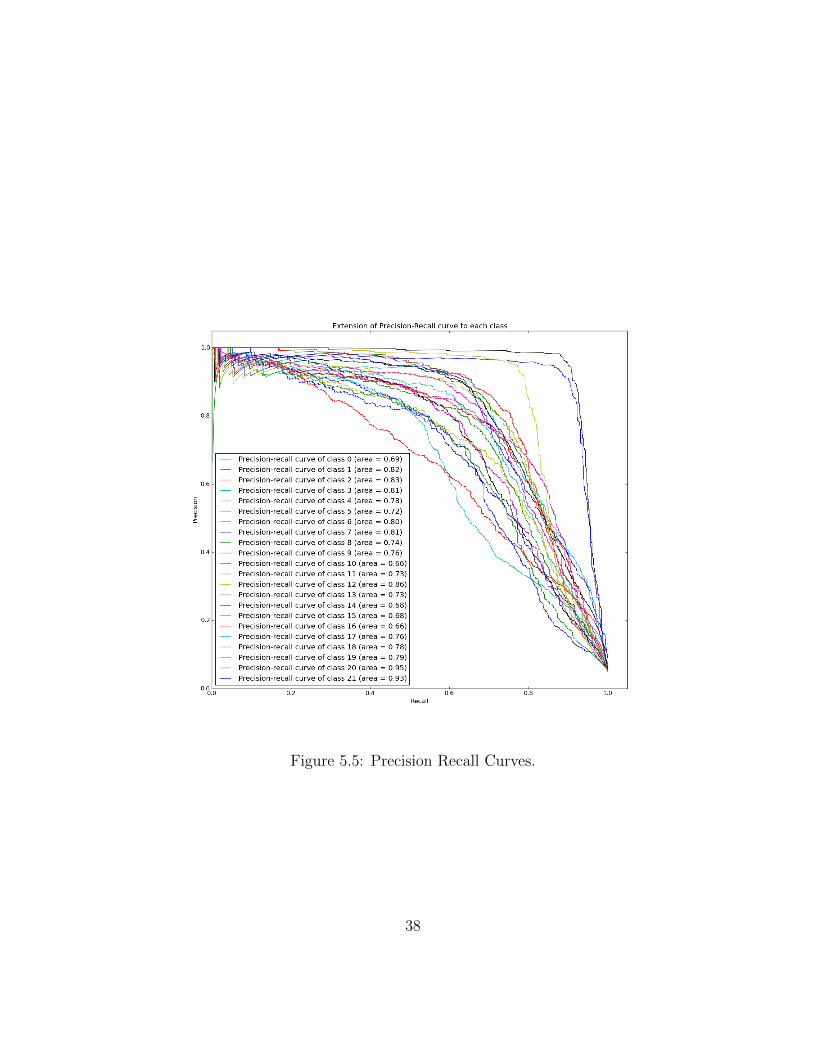
Figure 5.5: Precision Recall Curves.
38
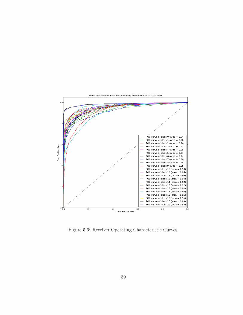
Figure 5.6: Receiver Operating Characteristic Curves.
39

no longer capable of learning all the information, thus we need to increase the number ofparameters in the network, so our experiments compared performance of models with dif-ferent number of parameters. Tradeo↵ between performance and e�ciency was a criterionin choosing models.
40
Chapter 6
Conclusions
6.1 Summary
This thesis defines a multi–label classification problem for extracting the relation candidatesfrom a question. We propose two deep learning methods, Parallel CNN and Deep CNN, topredict multiple relation candidates of a question. Parallel CNN consists of four parallelconvolutional layers, while Deep CNN has two stacked convolutional layers. Convolutionallayers of both the models capture local semantic features. A max over time pooling layer isplaced on top of the last convolutional layer to select global semantic features, followed by afully connected layer with dropout to summarize the features. Our experiments show thatboth Parallel and Deep CNN outperform the traditional Support Vector Classification(SVC)–based method by a large margin. Furthermore, we observe that Deep CNN hasbetter performance than Parallel CNN, indicating that the deep structure enables muchstronger semantic learning capacity than the wide but shallow network. Our method laysa firm foundation for implementing a high performance QA system.
6.2 Future Work
In this work, we chose several hundreds of most frequently appeared relations as our target.However, the overall dataset contains more than 19,000 relations and many of them arerarely present. The limitation of our model is that it is impossible to adapt our CNNsfor the 19,000 relations recognition problem by simply adding more output neurons. One
41
possible solution could be first hierarchically clustering all the relations, and then usingcascade network classifiers for each cluster.
On the other hand, the word2vec model we used in this work was trained on theGoogle News corpus. As shown in [50], the word2vec space trained in social media corpusis di↵erent from that in carefully edited prose. Thus, we could retrain the word2vec on theWikiAnswer corpus toward improving our performance.
In summary, we conclude that following steps to complete a KB–supported QA systemare needed:
• Map the relations predicted by the model to those used in the knowledge database,such as DBpedia or Freebase (o✏ine).
• Recognize the entities with POS tagging, or NER, or other NLP tools.
• Query the database with the entities and mapped relations.
• Retrieve the answer from the database and generate a sentence accordingly.
42
APPENDICES
43
Appendix A
Python Implementation for BuildingCNNs
A.1 Deep CNN
def Deep_CNN ():
#Two Convolutional Layers with Pooling Layer
model = Sequential ()
model.add(Convolution2D(27, 1, 3, 1, border_mode=’valid ’, activation=’
relu’))
model.add(Convolution2D(2048 , 27, 3, 300 , border_mode=’valid ’,
activation=’relu’))
model.add(MaxPooling2D(poolsize=(21, 1)))
#Fully Connected Layer with dropout
model.add(Flatten ())
model.add(Dense(2048 , 256 , activation=’relu’))
model.add(Dropout(0.5))
#Fully Connected Layer as output layer
model.add(Dense(256 , len(label_set), activation=’sigmoid ’))
adadelta = Adadelta(lr=1.0, rho=0.95, epsilon=1e-6)
model.compile(loss=’binary_crossentropy ’, class_mode=’multi_label ’,
optimizer=adadelta)
44

A.2 Parallel CNN
def Deep_CNN ():
filter_shapes = [[2, 300], [3, 300], [4, 300], [5, 300]]
pool_shapes = [[25, 1], [24, 1], [23, 1], [22, 1]]
#Four Parallel Convolutional Layers with Four Pooling Layers
model = Sequential ()
sub_models = []
for i in range(len(pool_shapes)):
pool_shape = pool_shapes[i]
filter_shape = filter_shapes[i]
sub_model = Sequential ()
sub_model.add(Convolution2D(512 1, filter_shape[0], filter_shape[
1], border_mode=’valid ’,
activation=’relu’))
sub_model.add(MaxPooling2D(poolsize=(pool_shape[0], pool_shape[1]
)))
sub_models.append(sub_model)
model.add(( Merge(sub_models , mode=’concat ’)))
#Fully Connected Layer with dropout
model.add(Flatten ())
model.add(Dense(2048 , 256 , activation=’relu’))
model.add(Dropout(0.5))
#Fully Connected Layer as output layer
model.add(Dense(256 , len(label_set), activation=’sigmoid ’))
adadelta = Adadelta(lr=1.0, rho=0.95, epsilon=1e-6)
model.compile(loss=’binary_crossentropy ’, class_mode=’multi_label ’,
optimizer=adadelta)
45
References
[1] Dbpedia website. http://wiki.dbpedia.org/.
[2] Freebase website. http://www.freebase.com.
[3] Keras website. http://keras.io/.
[4] scikit-learn website. http://scikit-learn.org/dev/index.html.
[5] Frederic Bastien, Pascal Lamblin, Razvan Pascanu, James Bergstra, Ian J. Goodfellow,Arnaud Bergeron, Nicolas Bouchard, and Yoshua Bengio. Theano: new features andspeed improvements. Deep Learning and Unsupervised Feature Learning NIPS 2012Workshop, 2012.
[6] Sven Behnke. Hierarchical neural networks for image interpretation, volume 2766.Springer Science & Business Media, 2003.
[7] James Bergstra, Olivier Breuleux, Frederic Bastien, Pascal Lamblin, Razvan Pas-canu, Guillaume Desjardins, Joseph Turian, David Warde-Farley, and Yoshua Bengio.Theano: a CPU and GPU math expression compiler. In Proceedings of the Pythonfor Scientific Computing Conference (SciPy), June 2010. Oral Presentation.
[8] Dan Ciresan, Ueli Meier, and Jurgen Schmidhuber. Multi-column deep neural net-works for image classification. In Computer Vision and Pattern Recognition (CVPR),2012 IEEE Conference on, pages 3642–3649. IEEE, 2012.
[9] Ronan Collobert and Jason Weston. A unified architecture for natural language pro-cessing: Deep neural networks with multitask learning. In Proceedings of the 25thInternational Conference on Machine Learning, ICML ’08, pages 160–167, New York,NY, USA, 2008. ACM.
46
[10] Ronan Collobert, Jason Weston, Leon Bottou, Michael Karlen, Koray Kavukcuoglu,and Pavel Kuksa. Natural language processing (almost) from scratch. J. Mach. Learn.Res., 12:2493–2537, November 2011.
[11] George Dahl, Dong Yu, Li Deng, and Alex Acero. Context-dependent pre-traineddeep neural networks for large-vocabulary speech recognition. IEEE Transactionson Audio, Speech, and Language Processing (receiving 2013 IEEE SPS Best PaperAward), 20(1):30–42, January 2012.
[12] Steven B. Damelin and Jr Willard Miller. The mathematics of signal processing. page232. Cambridge University Press, 2011.
[13] Cıcero Nogueira dos Santos and Maıra Gatti. Deep convolutional neural networks forsentiment analysis of short texts. In Proceedings of the 25th International Conferenceon Computational Linguistics (COLING), 2014.
[14] Cıcero Nogueira dos Santos, Bing Xiang, and Bowen Zhou. Classifying relations byranking with convolutional neural networks. In Proceedings of 53rd Annual Meetingof the Association for Computational Linguistics, pages 626–634, 2015.
[15] Anthony Fader, Stephen Soderland, and Oren Etzioni. Identifying relations for openinformation extraction. In Proceedings of the Conference on Empirical Methods inNatural Language Processing, pages 1535–1545. Association for Computational Lin-guistics, 2011.
[16] Anthony Fader, Luke Zettlemoyer, and Oren Etzioni. Paraphrase-driven learning foropen question answering. In Proceedings of the 51st Annual Meeting of the Associa-tion for Computational Linguistics (Volume 1: Long Papers), pages 1608–1618, Sofia,Bulgaria, August 2013. Association for Computational Linguistics.
[17] Jenny Rose Finkel, Trond Grenager, and Christopher Manning. Incorporating non-local information into information extraction systems by gibbs sampling. In Proceed-ings of the 43rd Annual Meeting on Association for Computational Linguistics, ACL’05, pages 363–370, Stroudsburg, PA, USA, 2005. Association for Computational Lin-guistics.
[18] Kunihiko Fukushima. Neocognitron: A self-organizing neural network model for amechanism of pattern recognition una↵ected by shift in position. Biological cybernet-ics, 36(4):193–202, 1980.
47

[19] The Stanford Natural Language Processing Group. Stanford named entity recognizer(ner). http://nlp.stanford.edu/software/CRF-NER.shtml.
[20] Iris Hendrickx, Su Nam Kim, Zornitsa Kozareva, Preslav Nakov, DiarmuidO Seaghdha, Sebastian Pado, Marco Pennacchiotti, Lorenza Romano, and Stan Sz-pakowicz. Semeval-2010 task 8: Multi-way classification of semantic relations betweenpairs of nominals. In Proceedings of the Workshop on Semantic Evaluations: RecentAchievements and Future Directions, pages 94–99. Association for Computational Lin-guistics, 2009.
[21] Geo↵rey Hinton, Li Deng, Dong Yu, George E Dahl, Abdel-rahman Mohamed,Navdeep Jaitly, Andrew Senior, Vincent Vanhoucke, Patrick Nguyen, Tara N Sainath,et al. Deep neural networks for acoustic modeling in speech recognition: The sharedviews of four research groups. Signal Processing Magazine, IEEE, 29(6):82–97, 2012.
[22] Baotian Hu, Zhengdong Lu, Hang Li, and Qingcai Chen. Convolutional neural net-work architectures for matching natural language sentences. In Advances in NeuralInformation Processing Systems, pages 2042–2050, 2014.
[23] Minqing Hu and Bing Liu. Mining and summarizing customer reviews. In Proceedingsof the Tenth ACM SIGKDD International Conference on Knowledge Discovery andData Mining, KDD ’04, pages 168–177, New York, NY, USA, 2004. ACM.
[24] Peter Jackson and Isabelle Moulinier. Natural language processing for online ap-plications: Text retrieval, extraction and categorization, volume 5. John BenjaminsPublishing, 2007.
[25] Nal Kalchbrenner, Edward Grefenstette, and Phil Blunsom. A convolutional neu-ral network for modelling sentences. Proceedings of the 52nd Annual Meeting of theAssociation for Computational Linguistics, June 2014.
[26] Andrej Karpathy. Stanford cs231n: Convolutional neural networks for visual recogni-tion. http://cs231n.github.io/.
[27] Yoon Kim. Convolutional neural networks for sentence classification. In Conferenceon Empirical Methods in Natural Language Processing, Doha, Qatar, 2014.
[28] LISA lab. Theano website. http://deeplearning.net/software/theano/index.
html, 2015.
48

[29] Quoc V. Le, Navdeep Jaitly, and Geo↵rey E. Hinton. A simple way to initializerecurrent networks of rectified linear units. CoRR, abs/1504.00941, 2015.
[30] Yann LeCun, Leon Bottou, Yoshua Bengio, and Patrick Ha↵ner. Gradient-basedlearning applied to document recognition. Proceedings of the IEEE, 86(11):2278–2324,1998.
[31] David D Lewis, Yiming Yang, Tony G Rose, and Fan Li. Rcv1: A new benchmarkcollection for text categorization research. The Journal of Machine Learning Research,5:361–397, 2004.
[32] Xin Li and Dan Roth. Learning question classifiers. In Proceedings of the 19th Inter-national Conference on Computational Linguistics - Volume 1, COLING ’02, pages1–7, Stroudsburg, PA, USA, 2002. Association for Computational Linguistics.
[33] Tomas Mikolov, Kai Chen, Greg Corrado, and Je↵rey Dean. E�cient estimation ofword representations in vector space. CoRR, abs/1301.3781, 2013.
[34] Tomas Mikolov, Martin Karafiat, Lukas Burget, Jan Cernocky, and Sanjeev Khudan-pur. Recurrent neural network based language model. In INTERSPEECH 2010,11th Annual Conference of the International Speech Communication Association,Makuhari, Chiba, Japan, September 26-30, 2010, pages 1045–1048, 2010.
[35] Tomas Mikolov, Ilya Sutskever, Kai Chen, Greg Corrado, and Je↵rey Dean. Dis-tributed representations of words and phrases and their compositionality. CoRR,abs/1310.4546, 2013.
[36] Tomas Mikolov, Wen tau Yih, and Geo↵rey Zweig. Linguistic regularities in contin-uous space word representations. In Proceedings of the 2013 Conference of the NorthAmerican Chapter of the Association for Computational Linguistics: Human Lan-guage Technologies (NAACL-HLT-2013). Association for Computational Linguistics,May 2013.
[37] Andrew Ng, Jiquan Ngiam, Chuan Yu Foo, Yifan Mai, Caroline Suen, Adam Coates,Andrew Maas, Awni Hannun, Brody Huval, Tao Wang, and Sameep Tandon. Ufldltutorial. http://ufldl.stanford.edu/tutorial/.
[38] Peter Norvig. Spelling corrector. http://norvig.com/spell-correct.html.
[39] Bo Pang and Lillian Lee. A sentimental education: Sentiment analysis using sub-jectivity summarization based on minimum cuts. In Proceedings of the 42nd Annual
49
Meeting on Association for Computational Linguistics, ACL ’04, Stroudsburg, PA,USA, 2004. Association for Computational Linguistics.
[40] Bo Pang and Lillian Lee. Seeing stars: Exploiting class relationships for sentimentcategorization with respect to rating scales. In Proceedings of the 43rd Annual Meetingon Association for Computational Linguistics, pages 115–124. Association for Com-putational Linguistics, 2005.
[41] Razvan Pascanu, Tomas Mikolov, and Yoshua Bengio. Understanding the explodinggradient problem. CoRR, abs/1211.5063, 2012.
[42] Vasile Rus, Philip MMcCarthy, Mihai C Lintean, Danielle S McNamara, and Arthur CGraesser. Paraphrase identification with lexico-syntactic graph subsumption. InFLAIRS conference, pages 201–206, 2008.
[43] Cicero D. Santos and Bianca Zadrozny. Learning character-level representations forpart-of-speech tagging. In Tony Jebara and Eric P. Xing, editors, Proceedings ofthe 31st International Conference on Machine Learning (ICML-14), pages 1818–1826.JMLR Workshop and Conference Proceedings, 2014.
[44] Yelong Shen, Xiaodong He, Jianfeng Gao, Li Deng, and Gregoire Mesnil. Learn-ing semantic representations using convolutional neural networks for web search. InProceedings of the 23rd International Conference on World Wide Web, WWW ’14Companion, pages 373–374, Republic and Canton of Geneva, Switzerland, 2014. In-ternational World Wide Web Conferences Steering Committee.
[45] Patrice Y. Simard, Dave Steinkraus, and John C. Platt. Best practices for convo-lutional neural networks applied to visual document analysis. In Proceedings of theSeventh International Conference on Document Analysis and Recognition - Volume 2,ICDAR ’03, pages 958–, Washington, DC, USA, 2003. IEEE Computer Society.
[46] Richard Socher, John Bauer, Christopher D. Manning, and Andrew Y. Ng. Parsingwith compositional vector grammars. In Proceedings of the ACL conference, 2013.
[47] Richard Socher, Brody Huval, Christopher D. Manning, and Andrew Y. Ng. Se-mantic compositionality through recursive matrix-vector spaces. In Proceedings ofthe 2012 Joint Conference on Empirical Methods in Natural Language Processing andComputational Natural Language Learning, EMNLP-CoNLL ’12, pages 1201–1211,Stroudsburg, PA, USA, 2012. Association for Computational Linguistics.
50

[48] Richard Socher, Alex Perelygin, Jean Y Wu, Jason Chuang, Christopher D Manning,Andrew Y Ng, and Christopher Potts. Recursive deep models for semantic compo-sitionality over a sentiment treebank. In Proceedings of the Conference on EmpiricalMethods in Natural Language Processing (EMNLP), volume 1631, page 1642, 2013.
[49] Nitish Srivastava, Geo↵rey Hinton, Alex Krizhevsky, Ilya Sutskever, and RuslanSalakhutdinov. Dropout: A simple way to prevent neural networks from overfitting.Journal of Machine Learning Research, 15:1929–1958, 2014.
[50] Luchen Tan, Haotian Zhang, Charles L.A. Clarke, and Mark D. Smucker. Lexicalcomparison between wikipedia and twitter corpora by using word embeddings. InProceedings of ACL, Beijing, China, June 2015. Association for Computational Lin-guistics.
[51] Wen tau Yih, Xiaodong He, and Christopher Meek. Semantic parsing for single-relation question answering. In Proceedings of ACL. Association for ComputationalLinguistics, June 2014.
[52] Janyce Wiebe, Theresa Wilson, and Claire Cardie. Annotating expressions of opinionsand emotions in language. Language Resources and Evaluation, 39(2-3):165–210, 2005.
[53] Mo Yu, Matthew Gormley, and Mark Dredze. Factor-based compositional embeddingmodels. In NIPS Workshop on Learning Semantics, 2014.
[54] Matthew D. Zeiler. Adadelta: An adaptive learning rate method. CoRR,abs/1212.5701, 2012.
[55] Daojian Zeng, Kang Liu, Siwei Lai, Guangyou Zhou, and Jun Zhao. Relation clas-sification via convolutional deep neural network. In Proceedings of COLING, pages2335–2344, Dublin, Ireland, 2014.
51