1

Convolutional Recurrent Neural Networks forDynamic MR Image Reconstruction

Chen Qin*†, Jo Schlemper*, Jose Caballero, Anthony N. Price, Joseph V. Hajnal and DanielRueckert Fellow, IEEE

Abstract—Accelerating the data acquisition of dynamic mag-netic resonance imaging (MRI) leads to a challenging ill-posedinverse problem, which has received great interest from both thesignal processing and machine learning communities over thelast decades. The key ingredient to the problem is how to exploitthe temporal correlations of the MR sequence to resolve aliasingartefacts. Traditionally, such observation led to a formulationof an optimisation problem, which was solved using iterativealgorithms. Recently, however, deep learning based-approacheshave gained significant popularity due to their ability to solve gen-eral inverse problems. In this work, we propose a unique, novelconvolutional recurrent neural network (CRNN) architecturewhich reconstructs high quality cardiac MR images from highlyundersampled k-space data by jointly exploiting the dependenciesof the temporal sequences as well as the iterative nature of thetraditional optimisation algorithms. In particular, the proposedarchitecture embeds the structure of the traditional iterativealgorithms, efficiently modelling the recurrence of the iterativereconstruction stages by using recurrent hidden connectionsover such iterations. In addition, spatio-temporal dependenciesare simultaneously learnt by exploiting bidirectional recurrenthidden connections across time sequences. The proposed methodis able to learn both the temporal dependency and the iterativereconstruction process effectively with only a very small numberof parameters, while outperforming current MR reconstructionmethods in terms of reconstruction accuracy and speed.

Index Terms—Recurrent neural network, convolutional neuralnetwork, dynamic magnetic resonance imaging, cardiac imagereconstruction

I. INTRODUCTION

MAGNETIC Resonance Imaging (MRI) is a non-invasiveimaging technique which offers excellent spatial reso-

lution and soft tissue contrast and is widely used for clinicaldiagnosis and research. Dynamic MRI attempts to reveal bothspatial and temporal profiles of the underlying anatomy, whichhas a variety of applications such as cardiovascular imagingand perfusion imaging. However, the acquisition speed isfundamentally limited due to both hardware and physiologicalconstraints as well as the requirement to satisfy the Nyquistsampling rate. Long acquisition times are not only a burdenfor patients but also make MRI susceptible to motion artefacts.

This work was supported by EPSRC programme grant SmartHeart(EP/P001009/1). C. Qin is supported by China Scholarship Council (CSC).†Corresponding author: Chen Qin. (Email address: c.qin15@imperial.ac.uk)*These authors contributed equally to this work.C. Qin, J. Schlemper, J. Caballero and D. Rueckert are with the Biomedical

Image Analysis Group, Department of Computing, Imperial College London,SW7 2AZ London, UK.

J. V. Hajnal, and A. N. Price are with with the Division of Imaging Sciencesand Biomedical Engineering Department, King’s College London, St. Thomas’Hospital, SE1 7EH London, U.K.

In order to accelerate MRI acquisition, most approachesconsider undersampling the data in k-space (frequency do-main). Due to the violation of the Nyquist sampling theorem,undersampling introduces aliasing artefacts in the imagedomain. Images can be subsequently reconstructed by solvingan optimisation problem that regularises the solution withassumptions on the underlying data, such as smoothness,sparsity or, for the case of dynamic imaging, spatio-temporalredundancy. Past literature has shown that exploiting spatio-temporal redundancy can greatly improve image reconstructionquality compared to compressed sensing (CS) based singleframe reconstruction methods [1], [2]. However, the challengesof these optimisation based approaches are the following: firstly,the regularisation functions and their hyper-parameters must becarefully selected, which are problem-specific and non-trivial.For example, over-imposing sparsity or `1 penalties can leadto cartoon-like/staircase artefacts. Secondly, the reconstructionspeeds of these methods are often slow due to requirement tosolve iterative algorithms. Proposing a robust iterative algorithmis still an active area of research.

In comparison, deep learning methods are gaining popularityfor their accuracy and efficiency. Unlike traditional approaches,the prior information and regularisation are learnt implicitlyfrom data, without having to specify them in the trainingobjective. However, so far only a handful of approaches exist[3], [4] for dynamic reconstruction. Hence, the applicability ofdeep learning models to this problem is yet to be fully explored.In addition, many proposed deep learning architectures areoften generic and are not optimised for specific applications.In particular, a core question for dynamic reconstructionis how to optimally exploit spatio-temporal redundancy. Bydesigning a network architecture and regulating the mechanicsof network layers to efficiently learn such spatio-temporaldata representation, the network should gain a boost inperformances.

In this work, we propose a novel convolutional recurrentneural network (CRNN) method to reconstruct high qualitydynamic MR image sequences from undersampled data, termedCRNN-MRI. Firstly, we formulate a general optimisationproblem for solving accelerated dynamic MRI based onvariable splitting and alternate minimisation. We then showhow this algorithm can be seen as a network architecture.In particular, the proposed method consists of a CRNN blockwhich acts as the proximal operator and a data consistency layercorresponding to the classical data fidelity term. In addition,the CRNN block employs recurrent connections across eachiteration step, allowing reconstruction information to be shared

Copyright c© 2017 IEEE. Personal use of this material is permitted. However, permission to use this material for any other purposes must be obtained from theIEEE by sending a request to pubs-permissions@ieee.org.

arX

iv:1

712.

0175

1v3

[cs

.CV

] 1

4 O

ct 2

018

2

across the multiple iterations of the process. Secondly, weincorporate bidirectional convolutional recurrent units evolvingover time to exploit the temporal dependency of the dynamicsequences and effectively propagate the contextual informationacross time frames of the input. As a consequence, the uniqueCRNN architecture jointly learns representations in a recurrentfashion evolving over both time sequences as well as iterationsof the reconstruction process, effectively combining the benefitsof traditional iterative methods and deep learning.

To the best of our knowledge, this is the first work applyingRNNs for dynamic MRI reconstruction. The contributions ofthis work are the following: Firstly, we view the optimisationproblem of dynamic data as a recurrent network and describea novel CRNN architecture which simultaneously incorporatesthe recurrence existing in both temporal and iteration sequentialsteps. Secondly, we demonstrate that the proposed methodshows promising results and improves upon the currentstate-of-the-art dynamic MR reconstruction methods both inreconstruction accuracy and speed. Finally, we compare ourarchitecture to 3D CNN which does not impose the recurrentstructure. We show that the proposed method outperformsthe CNN at different undersampling rates and speed, whilerequiring significantly fewer parameters.

II. RELATED WORK

One of the main challenges associated with recovering anuncorrupted image is that both the undersampling strategyand a-priori knowledge of appropriate properties of the imageneed to be taken into account. Methods like k-t BLAST andk-t SENSE [5] take advantage of a-priori information aboutthe x-f support obtained from the training data set in orderto prune a reconstruction to optimally reduce aliasing. Analternative popular approach is to exploit temporal redundancyto unravel from the aliasing by using CS approaches [1], [6] orCS combined with low-rank approaches [2], [7]. The class ofmethods which employ CS to the MRI reconstruction is termedas CS-MRI [8]. They assume that the image to be reconstructedhas a sparse representation in a certain transform domain, andthey need to balance sparsity in the transform domain againstconsistency with the acquired undersampled k-space data. Forinstance, an example of successful methods enforcing sparsityin x-f domain is k-t FOCUSS [1]. A low rank and sparsereconstruction scheme (k-t SLR) [2] introduces non-convexspectral norms and uses a spatio-temporal total variation normin recovering the dynamic signal matrix. Dictionary learningapproaches were also proposed to train an over-complete basisof atoms to optimally sparsify spatio-temporal data [6]. Thesemethods offer great potential for accelerated imaging, however,they often impose strong assumptions on the underlying data,requiring nontrivial manual adjustments of hyperparametersdepending on the application. In addition, it has been observedthat these methods tend to result in blocky [9] and unnaturalreconstructions, and their reconstruction speed is often slow.Furthermore, these methods are not able to exploit the priorknowledge that can be learnt from the vast number of MRIexams routinely performed, which should be helpful to furtherguide the reconstruction process.

Recently, deep learning-based MR reconstruction has gainedpopularity due to its promising results for solving inverse andcompressed sensing problems. In particular, two paradigmshave emerged: the first class of approaches proposes to useconvolutional neural networks (CNNs) to learn an end-to-endmapping, where architectures such as SRCNN [10] or U-net[11] are often chosen for MR image reconstruction [12], [13],[14], [15]. The second class of approaches attempts to makeeach stage of iterative optimisation learnable by unrolling theend-to-end pipeline into a deep network [9], [16], [17], [18],[19]. For instance, Hammernik et al. [9] introduced a trainableformulation for accelerated parallel imaging (PI) based MRIreconstruction termed variational network, which embedded aCS concept within a deep learning approach. ADMM-Net [17]was proposed by reformulating an alternating direction methodof multipliers (ADMM) algorithm to a deep network, whereeach stage of the architecture corresponds to an iteration inthe ADMM algorithm. More recently, Schlemper et al. [18]proposed a cascade network which simulated the iterativereconstruction of dictionary learning-based methods and werelater extended for dynamic MR reconstructions [3]. Mostapproaches so far have focused on 2D images, whereas only afew approaches exist for dynamic MR reconstruction [3], [4].While they show promising results, the optimal architecture,training scheme and configuration spaces are yet to be fullyexplored.

More recently, several methods on 2D MR image recon-struction were proposed [9], [20], [21], which share similaridea with our proposed method that integrates data fidelityterm and regularisation term into a single deep network sothat to enable the end-to-end training. In contrast to thesemethods which use shared parameters over iterations, as wewill show, our architecture integrates hidden connections overoptimisation iterations to propagate learnt representations acrossboth iteration and time, whereas such information is discardedin the other methods. Such proposed architecture enables theinformation used for the reconstruction at each iteration to beshared across all stages of the reconstruction process, aiming foran iterative algorithm that can fully benefit from informationextracted at all processing stages. As to the nature of theproposed RNN units, previous work involving RNNs onlyupdated the hidden state of the recurrent connection with afixed input [22], [23], [24], while the proposed architectureprogressively updates the input as the optimisation iterationincreases. In addition, previous work only modelled therecurrence of iteration or time [25] exclusively, whereas theproposed method jointly exploits both dimensions, yieldinga unique architecture suitable for the dynamic reconstructionproblem.

III. CONVOLUTIONAL RECURRENT NEURAL NETWORKFOR MRI RECONSTRUCTION

A. Problem Formulation

Let x ∈ CD denote a sequence of complex-valued MRimages to be reconstructed, represented as a vector withD = DxDyT , and let y ∈ CM (M << D) represent theundersampled k-space measurements, where Dx and Dy are

3

width and height of the frame respectively and T standsfor the number of frames. Our problem is to reconstruct xfrom y, which is commonly formulated as an unconstrainedoptimisation problem of the form:

argminx

R(x) + λ‖y − Fux‖22 (1)

Here Fu is an undersampling Fourier encoding matrix, Rexpresses regularisation terms on x and λ allows the adjustmentof data fidelity based on the noise level of the acquiredmeasurements y. For CS and low-rank based approaches, theregularisation terms R often employed are `0 or `1 norms inthe sparsifying domain of x as well as the rank or nuclearnorm of x respectively. In general, Eq. 1 is a non-convexfunction and hence, the variable splitting technique is usuallyadopted to decouple the fidelity term and the regularisationterm. By introducing an auxiliary variable z that is constrainedto be equal to x, Eq. 1 can be reformulated to minimize thefollowing cost function via the penalty method:

argminx,z

R(z) + λ‖y − Fux‖22 + µ‖x− z‖22 (2)

where µ is a penalty parameter. By applying alternate minimi-sation over x and z, Eq. 2 can be solved via the followingiterative procedures:

z(i+1) = argminzR(z) + µ‖x(i) − z‖22 (3a)

x(i+1) = argminx

λ‖y − Fux‖22 + µ‖x− z(i+1)‖22 (3b)

where x(0) = xu = FHu y is the zero-filled reconstruction takenas an initialisation and z can be seen as an intermediate stateof the optimisation process. For MRI reconstruction, Eq. 3b isoften regarded as a data consistency (DC) step where we canobtain the following closed-form solution [18]:

x(i+1) = DC(z(i); y, λ0,Ω) = FHΛFz(i) + λ0

1+λ0FHu y,

Λkk =

1 if k 6∈ Ω

11+λ0

if k ∈ Ω(4)

in which F is the full Fourier encoding matrix (a discreteFourier transform in this case), λ0 = λ/µ is a ratio ofregularization parameters from Eq. 4, Ω is an index set of theacquired k-space samples and Λ is a diagonal matrix. Pleaserefer to [18] for more details of formulating Eq. 4 as a dataconsistency layer in a neural network. Eq. 3a is the proximaloperator of the prior R, and instead of explicitly determiningthe form of the regularisation term, we propose to directlylearn the proximal operator by using a convolutional recurrentneural network (CRNN).

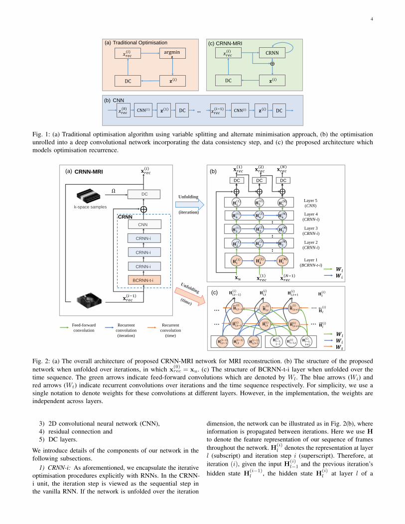
Previous deep learning approaches such as Deep-ADMM net[17] and method proposed by Schlemper et al. [18] unroll thetraditional optimisation algorithm. Hence, their models learn asequence of transition x(0) → z(1) → x(1) → · · · → z(N) →x(N) to reconstruct the image, where each state transition atstage (i) is an operation such as convolutions independentlyparameterised by θ, nonlinearities or a data consistency step.However, since the network implicitly learns some form ofproximal operator at each iteration, it may be redundant to

individually parameterise each step. In our formulation, wemodel each optimisation stage (i) as a learnt, recurrent, forwardencoding step fi(x

(i−1), z(i−1);θ,y, λ,Ω). The differenceis that now we use one model which performs proximaloperator, however, it also allows itself to propagate informationacross iteration, making it adaptable for the changes across theoptimisation steps. The detail will be discussed in the followingsection. The different strategies are illustrated in Fig 1.

B. CRNN for MRI reconstruction

RNN is a class of neural networks that makes use ofsequential information to process sequences of inputs. Theymaintain an internal state of the network acting as a "memory",which allows RNNs to naturally lend themselves to theprocessing of sequential data. Inspired by iterative optimisationschemes of Eq. 3, we propose a novel convolutional RNN(CRNN) network. In the most general scope, our neuralencoding model is defined as follows,

xrec = fN (fN−1(· · · (f1(xu)))), (5)

in which xrec denotes the prediction of the network, xu is thesequence of undersampled images with length T and also theinput of the network, fi(xu;θ, λ,Ω) is the network functionfor each iteration of optimisation step, and N is the numberof iterations. We can compactly represent a single iteration fiof our network as follows:

x(i)rnn = x(i−1)

rec + CRNN(x(i−1)rec ), (6a)

x(i)rec = DC(x(i)

rnn; y, λ0,Ω), (6b)

where CRNN is a learnable block explained hereafter, DCis the data consistency step treated as a network layer, x

(i)rec

is the progressive reconstruction of the undersampled imagexu at iteration i with x

(0)rec = xu, x

(i)rnn is the intermediate

reconstruction image before the DC layer, and y is theacquired k-space samples. Note that the variables xrec,xrnn areanalogous to x, z in Eq. 3 respectively. Here, we use CRNNto encode the update step, which can be seen as one stepof a gradient descent in the sense of objective minimisation,or a more general approximation function regressing thedifference z(i+1) − x(i), i.e. the distance required to moveto the next state. Moreover, note that in every iteration,CRNN updates its internal state H given an input which isdiscussed shortly. As such, CRNN also allows information tobe propagated efficiently across iterations, in contrast to thesequential models using CNNs which collapse the intermediatefeature representation to z(i).

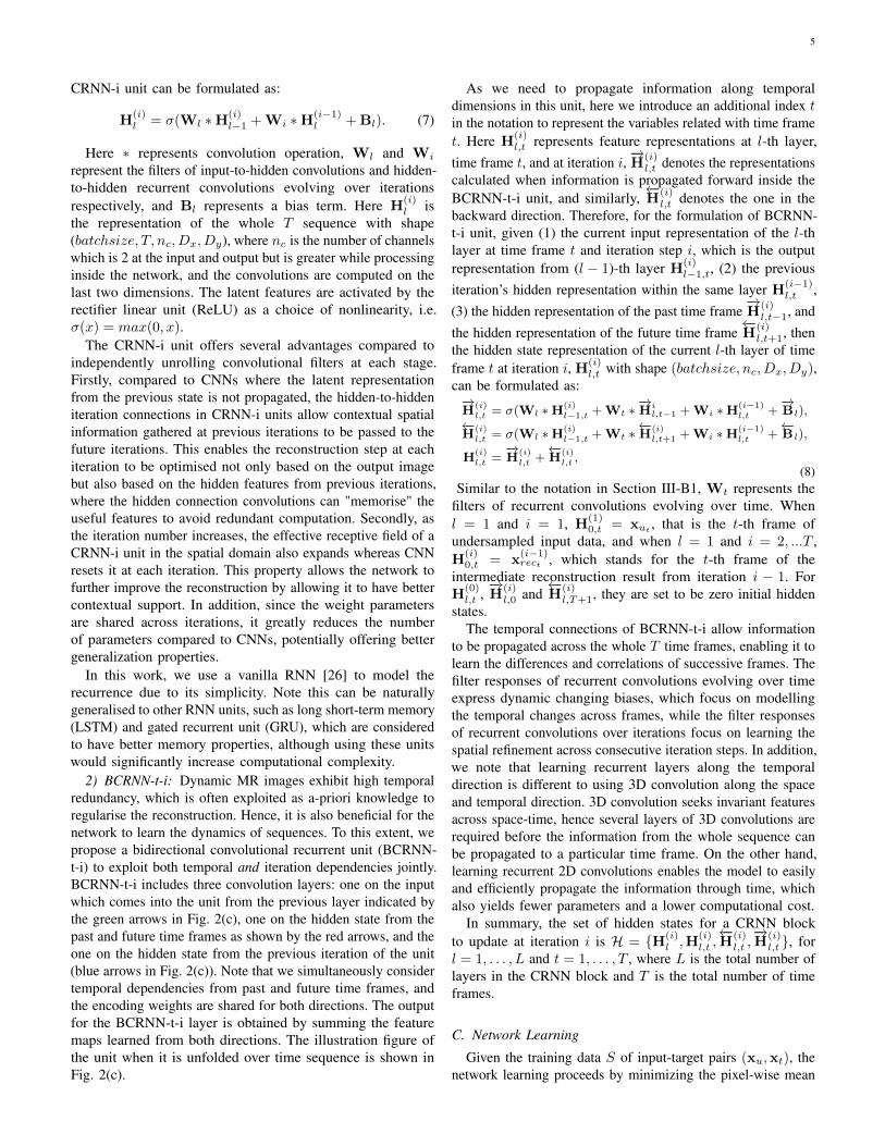
In order to exploit the dynamic nature and the temporalredundancy of our data, we further propose to jointly model therecurrence evolving over time for dynamic MRI reconstruction.The proposed CRNN-MRI network and CRNN block are shownin Fig. 2(a), in which CRNN block comprised of 5 components:

1) bidirectional convolutional recurrent units evolving overtime and iterations (BCRNN-t-i),

2) convolutional recurrent units evolving over iterations only(CRNN-i),

4

DC

𝑥𝑟𝑒𝑐(𝑖)

CNN(1) DC𝑥𝑟𝑒𝑐(0)

CRNN

DC

𝑥𝑟𝑒𝑐(𝑖)

CNN(i) DC𝑥𝑟𝑒𝑐(𝑖−1)…

CNN

Traditional Optimisation CRNN-MRI

⨁

(a)

(b)

(c)

argmin𝐳

𝐳 𝑖 𝐳 𝑖

𝐳 1 𝐳 𝑖

Fig. 1: (a) Traditional optimisation algorithm using variable splitting and alternate minimisation approach, (b) the optimisationunrolled into a deep convolutional network incorporating the data consistency step, and (c) the proposed architecture whichmodels optimisation recurrence.

CRNN-i

CNN

....

..

CRNN-i

CRNN-i

BCRNN-t-i

DC

𝐱𝑟𝑒𝑐1𝐱𝑢

𝐱𝑟𝑒𝑐𝑖 𝐱𝑟𝑒𝑐

1

𝐱𝑟𝑒𝑐𝑁−1

DC DC DC

𝐱𝑟𝑒𝑐2 𝐱𝑟𝑒𝑐

𝑁

Layer 1

(BCRNN-t-i)

Layer 2

(CRNN-i)

Layer 4

(CRNN-i)

Layer 3

(CRNN-i)

Unfolding

(iteration)

Feed-forward

convolution

Recurrent

convolution

(iteration)

Recurrent

convolution

(time)

(a) (b)

Layer 5

(CNN)

𝐱𝑟𝑒𝑐𝑖−1

k-space samples

Ω

𝐇1(1) 𝐇𝟏

(2)𝐇1(N)

𝐇2(1) 𝐇2

(2)𝐇2(N)

𝐇3(1) 𝐇3

(2)𝐇3(N)

𝐇4(1)

𝐇4(2)

𝐇4(N)

𝐇5(1) 𝐇5

(2)𝐇5(N)

⨁ ⨁ ⨁

⨁

…

…

…

… 𝐇𝑙𝑖

𝐇𝑙𝑖

𝐇 )𝑙,𝑡−1𝑖

𝐇𝑙,𝑡+1𝑖𝐇𝑙,𝑡

𝑖𝐇𝑙𝑖

𝐇𝑙,𝑡−1𝑖

𝐇𝑙,𝑡𝑖

𝐇𝑙,𝑡+1𝑖

𝐇𝑙,𝑡+1𝑖

𝐇𝑙,𝑡−1𝑖

𝐇𝑙,𝑡𝑖

𝐇𝑙,𝑡−1𝑖−1

𝐇𝑙,𝑡𝑖−1

𝐇𝑙,𝑡+1𝑖−1 𝐇𝑙−1,𝑡

𝑖𝐇𝑙−1,𝑡−1

𝑖𝐇𝑙−1,𝑡+1

𝑖

(c)

CRNN-MRI

CRNN

𝑾𝑙

𝑾𝑖

𝑾𝑡

𝑾𝑙

𝑾𝑖

Fig. 2: (a) The overall architecture of proposed CRNN-MRI network for MRI reconstruction. (b) The structure of the proposednetwork when unfolded over iterations, in which x

(0)rec = xu. (c) The structure of BCRNN-t-i layer when unfolded over the

time sequence. The green arrows indicate feed-forward convolutions which are denoted by Wl. The blue arrows (Wi) andred arrows (Wt) indicate recurrent convolutions over iterations and the time sequence respectively. For simplicity, we use asingle notation to denote weights for these convolutions at different layers. However, in the implementation, the weights areindependent across layers.

3) 2D convolutional neural network (CNN),4) residual connection and5) DC layers.

We introduce details of the components of our network in thefollowing subsections.

1) CRNN-i: As aforementioned, we encapsulate the iterativeoptimisation procedures explicitly with RNNs. In the CRNN-i unit, the iteration step is viewed as the sequential step inthe vanilla RNN. If the network is unfolded over the iteration

dimension, the network can be illustrated as in Fig. 2(b), whereinformation is propagated between iterations. Here we use Hto denote the feature representation of our sequence of framesthroughout the network. H

(i)l denotes the representation at layer

l (subscript) and iteration step i (superscript). Therefore, atiteration (i), given the input H

(i)l−1 and the previous iteration’s

hidden state H(i−1)l , the hidden state H

(i)l at layer l of a

5

CRNN-i unit can be formulated as:

H(i)l = σ(Wl ∗H

(i)l−1 + Wi ∗H

(i−1)l + Bl). (7)

Here ∗ represents convolution operation, Wl and Wi

represent the filters of input-to-hidden convolutions and hidden-to-hidden recurrent convolutions evolving over iterationsrespectively, and Bl represents a bias term. Here H

(i)l is

the representation of the whole T sequence with shape(batchsize, T, nc, Dx, Dy), where nc is the number of channelswhich is 2 at the input and output but is greater while processinginside the network, and the convolutions are computed on thelast two dimensions. The latent features are activated by therectifier linear unit (ReLU) as a choice of nonlinearity, i.e.σ(x) = max(0, x).

The CRNN-i unit offers several advantages compared toindependently unrolling convolutional filters at each stage.Firstly, compared to CNNs where the latent representationfrom the previous state is not propagated, the hidden-to-hiddeniteration connections in CRNN-i units allow contextual spatialinformation gathered at previous iterations to be passed to thefuture iterations. This enables the reconstruction step at eachiteration to be optimised not only based on the output imagebut also based on the hidden features from previous iterations,where the hidden connection convolutions can "memorise" theuseful features to avoid redundant computation. Secondly, asthe iteration number increases, the effective receptive field of aCRNN-i unit in the spatial domain also expands whereas CNNresets it at each iteration. This property allows the network tofurther improve the reconstruction by allowing it to have bettercontextual support. In addition, since the weight parametersare shared across iterations, it greatly reduces the numberof parameters compared to CNNs, potentially offering bettergeneralization properties.

In this work, we use a vanilla RNN [26] to model therecurrence due to its simplicity. Note this can be naturallygeneralised to other RNN units, such as long short-term memory(LSTM) and gated recurrent unit (GRU), which are consideredto have better memory properties, although using these unitswould significantly increase computational complexity.

2) BCRNN-t-i: Dynamic MR images exhibit high temporalredundancy, which is often exploited as a-priori knowledge toregularise the reconstruction. Hence, it is also beneficial for thenetwork to learn the dynamics of sequences. To this extent, wepropose a bidirectional convolutional recurrent unit (BCRNN-t-i) to exploit both temporal and iteration dependencies jointly.BCRNN-t-i includes three convolution layers: one on the inputwhich comes into the unit from the previous layer indicated bythe green arrows in Fig. 2(c), one on the hidden state from thepast and future time frames as shown by the red arrows, and theone on the hidden state from the previous iteration of the unit(blue arrows in Fig. 2(c)). Note that we simultaneously considertemporal dependencies from past and future time frames, andthe encoding weights are shared for both directions. The outputfor the BCRNN-t-i layer is obtained by summing the featuremaps learned from both directions. The illustration figure ofthe unit when it is unfolded over time sequence is shown inFig. 2(c).

As we need to propagate information along temporaldimensions in this unit, here we introduce an additional index tin the notation to represent the variables related with time framet. Here H

(i)l,t represents feature representations at l-th layer,

time frame t, and at iteration i,−→H

(i)l,t denotes the representations

calculated when information is propagated forward inside theBCRNN-t-i unit, and similarly,

←−H

(i)l,t denotes the one in the

backward direction. Therefore, for the formulation of BCRNN-t-i unit, given (1) the current input representation of the l-thlayer at time frame t and iteration step i, which is the outputrepresentation from (l − 1)-th layer H

(i)l−1,t, (2) the previous

iteration’s hidden representation within the same layer H(i−1)l,t ,

(3) the hidden representation of the past time frame−→H

(i)l,t−1, and

the hidden representation of the future time frame←−H

(i)l,t+1, then

the hidden state representation of the current l-th layer of timeframe t at iteration i, H

(i)l,t with shape (batchsize, nc, Dx, Dy),

can be formulated as:−→H

(i)l,t = σ(Wl ∗H(i)

l−1,t +Wt ∗−→Hi

l,t−1 +Wi ∗H(i−1)l,t +

−→B l),

←−H

(i)l,t = σ(Wl ∗H(i)

l−1,t +Wt ∗←−H

(i)l,t+1 +Wi ∗H(i−1)

l,t +←−B l),

H(i)l,t =

−→H

(i)l,t +

←−H

(i)l,t ,

(8)Similar to the notation in Section III-B1, Wt represents the

filters of recurrent convolutions evolving over time. Whenl = 1 and i = 1, H

(1)0,t = xut

, that is the t-th frame ofundersampled input data, and when l = 1 and i = 2, ...T ,H

(i)0,t = x

(i−1)rect , which stands for the t-th frame of the

intermediate reconstruction result from iteration i − 1. ForH

(0)l,t ,−→H

(i)l,0 and

←−H

(i)l,T+1, they are set to be zero initial hidden

states.The temporal connections of BCRNN-t-i allow information

to be propagated across the whole T time frames, enabling it tolearn the differences and correlations of successive frames. Thefilter responses of recurrent convolutions evolving over timeexpress dynamic changing biases, which focus on modellingthe temporal changes across frames, while the filter responsesof recurrent convolutions over iterations focus on learning thespatial refinement across consecutive iteration steps. In addition,we note that learning recurrent layers along the temporaldirection is different to using 3D convolution along the spaceand temporal direction. 3D convolution seeks invariant featuresacross space-time, hence several layers of 3D convolutions arerequired before the information from the whole sequence canbe propagated to a particular time frame. On the other hand,learning recurrent 2D convolutions enables the model to easilyand efficiently propagate the information through time, whichalso yields fewer parameters and a lower computational cost.

In summary, the set of hidden states for a CRNN blockto update at iteration i is H = H(i)

l ,H(i)l,t ,←−H

(i)l,t ,−→H

(i)l,t , for

l = 1, . . . , L and t = 1, . . . , T , where L is the total number oflayers in the CRNN block and T is the total number of timeframes.

C. Network Learning

Given the training data S of input-target pairs (xu,xt), thenetwork learning proceeds by minimizing the pixel-wise mean

6

squared error (MSE) between the predicted reconstructed MRimage and the fully sampled ground truth data:

L (θ) =1

nS

∑(xu,xt)∈S

‖xt − xrec‖22 (9)

where θ = Wl,Wi,Wt,Bl, l = 1 . . . L, and nS standsfor the number of samples in the training set S. Note thatthe total number of time sequences T and iteration steps Nassumed by the network before performing the reconstructionis a free parameter that must be specified in advance. Thenetwork weights were initialised using He initialization [27]and it was trained using the Adam optimiser [28]. Duringtraining, gradients were hard-clipped to the range of [−5, 5]to mitigate the gradient explosion problem. The network wasimplemented in Python using Theano and Lasagne libraries.

IV. EXPERIMENTS

A. Dataset and Implementation Details

The proposed method was evaluated using a complex-valued MR dataset consisting of 10 fully sampled short-axiscardiac cine MR scans. Each scan contains a single sliceSSFP acquisition with 30 temporal frames, which have a320 × 320 mm field of view and 10 mm thickness. Theraw data consists of 32-channel data with sampling matrixsize 192× 190, which was then zero-filled to the matrix size256 × 256. The raw multi-coil data was reconstructed usingSENSE [29] with no undersampling and retrospective gating.Coil sensitivity maps were normalized to a body coil imageand used to produce a single complex-valued reconstructedimage. In experiments, the complex valued images were back-transformed to regenerate k-space samples, simulating a fullysampled single-coil acquisition. The input undersampled imagesequences were generated by randomly undersampling thek-space samples using Cartesian undersampling masks, withundersampling patterns adopted from [1]: for each frame theeight lowest spatial frequencies were acquired, and the samplingprobability of k-space lines along the phase-encoding directionwas determined by a zero-mean Gaussian distribution. Notethat the undersampling rates are stated with respect to thematrix size of raw data, which is 192× 190.

The architecture of the proposed network used in theexperiment is shown in Fig. 2: each iteration of the CRNNblock contains five units: one layer of BCRNN-t-i, followedby three layers of CRNN-i units, and followed by a CNNunit. For all CRNN-i and BCRNN-t-i units, we used a kernelsize k = 3 and the number of filters was set to nf = 64 forProposed-A and nf = 128 for Proposed-B in Table I. The CNNafter the CRNN-i units contains one convolution layer withk = 3 and nf = 2, which projects the extracted representationback to the image domain which contains complex-valuedimages expressed using two channels. For all convolutionallayers, we used stride = 1 and paddings with half the filter size(rounded down) on both size. The output of the CRNN blockis connected to the residual connection, which sums the outputof the block with its input. Finally, we used DC layers on topof the CRNN output layers. During training, the iteration stepis set to be N = 10, and the time sequence for training is

T = 30. Note that this architecture is by no means optimaland more layers can be added to increase the ability of ournetwork to better capture the data structures (see Section IV-Dfor comparisons).

The evaluation was done via a 3-fold cross validation, wherefor two folds we train on 7 subjects then test on 3 subjects,and for the remaining fold we train on 6 subjects and test on 4subjects. While the original sequence has size 256× 256× T ,For the training, we extract patches of size 256×Dpatch × T ,where Dpatch = 32 is the patch size and the direction of patchextraction corresponds to the frequency-encoding direction.Note that since we only consider Cartesian undersampling,the aliasing occurs only along the phase encoding direction,so patch extraction does not alter the aliasing artefact. Patchextraction as well as data augmentation was performed on-the-fly, with random affine and elastic transformations on the imagedata. Undersampling masks were also generated randomlyfollowing patterns in [1] for each input. During test time, thenetwork trained on patches is directly applied on the wholesequence of the original image. The minibatch size during thetraining was set to 1, and we observed that the performancecan reach a plateau within 6× 104 backpropagations.

B. Evaluation Method

We compared the proposed method with the representativealgorithms of the CS-based dynamic MRI reconstruction, suchas k-t FOCUSS [1] and k-t SLR [2], and two variants of3D CNN networks named 3D CNN-S and 3D CNN in ourexperiments. The built baseline 3D CNN networks share thesame architecture with the proposed CRNN-MRI networkbut all the recurrent units and 2D CNN units were replacedwith 3D convolutional units, that is, in each iteration, the3D CNN block contain 5 layers of 3D convolutions, oneDC layer and a residual connection. Here 3D CNN-S refersto network sharing weights across iterations, however, thisdoes not employ the hidden-to-hidden connection as in theCRNN-i unit. The 3D CNN-S architecture was chosen so asto make a fair comparison with the proposed model using acomparable number of network parameters. In contrast, 3DCNN refers to the network without weight sharing, in whichthe network capacity is N = 10 times of that of 3D CNN-S, and approximately 12 times more than that of our firstproposed method (Proposed-A). For the 3D CNN approaches,the receptive field size is 11× 11× 11, as the receptive fieldsize is “reset” after each data consistency layer. In contrast, forthe proposed method, due to the hidden connections betweeniterations and bidirectional temporal connections, by tracing thelongest path of the convolution layers involved in the forwardpass, including both temporal and iterative directions, in theory,the receptive field size is 309× 309× 30 (154 layers of CNNsfor the middle frame in a sequence of 30 frames). However,the network still may predominantly relies on local featurescoming from the partial reconstruction. Nevertheless, the RNNhas the ability to exploit the features with larger filter size ifneeded, which is not the case for 3D CNNs.

Reconstruction results were evaluated based on the follow-ing quantitative metrics: MSE, peak-to-noise-ratio (PSNR),

7

structural similarity index (SSIM) [30] and high frequencyerror norm (HFEN) [31]. The choice of the these metrics wasmade to evaluate the reconstruction results with complimentaryemphasis. MSE and PSNR were chosen to evaluate the overallaccuracy of the reconstruction quality. SSIM put emphasison image quality perception. HFEN was used to quantify thequality of the fine features and edges in the reconstructions,and here we employed the same filter specification as in [31],[32] with the filter kernel size 15× 15 pixels and a standarddeviation of 1.5 pixels. For PSNR and SSIM, it is the higherthe better, while for MSE and HFEN, it is the lower the better.

C. Results

The comparison results of all methods are reported in Table I,where we evaluated the quantitative metrics, network capacityand reconstruction time. Numbers shown in Table I are meanvalues of corresponding metrics with standard deviation ofdifferent subjects in parenthesis. Bold numbers in Table Iindicate the better performance of the proposed methods thanthe competing ones. Compared with the baseline method (k-tFOCUSS and k-t SLR), the proposed methods outperform themby a considerable margin at different acceleration rates. Whencompared with deep learning methods, note that the networkcapacity of Proposed-A is comparable with that of 3D CNN-Sand the capacity of Propose-B is around one third of that of 3DCNN. Though their capacities are much smaller, both Proposed-A and Proposed-B outperform 3D CNN-S and 3D CNN forall acceleration rates by a large margin, which shows thecompetitiveness and effectiveness of our method. In addition,we can see a substantial improvement of the reconstructionresults on all acceleration rates and in all metrics when thenumber of network parameters is increased for the proposedmethod (Proposed-B), and therefore we will only show theresults from Proposed-B in the following. The number ofiterations used by the network at test time is set to be the sameas the training stage, which is N = 10, however, if the iterationnumber is increased up to N = 17, it shows an improvementof 0.324dB on average. Fig. 3 shows the model’s performancevarying with the number of iterations at test time. Similarly,visualization results of intermediate steps during the iterationsof a reconstruction from 9× undersampling data are shownin Fig. 4, where we can observe the gradual improvement ofthe reconstruction quality from iteration step 1 to 10, which isconsistent with the quantitative results as in Fig. 3.

A comparison of the visualization results of a reconstructionfrom 9× acceleration is shown in Fig. 5 with the reconstructedimages and their corresponding error maps from differentreconstruction methods. As one can see, our proposed model(Proposed-B) can produce more faithful reconstructions forthose parts of the image around the myocardium where thereare large temporal changes. This is reflected by the fact thatRNNs effectively use a larger receptive field to capture thecharacteristics of aliasing seen within the anatomy. Theirtemporal profiles at x = 120 are shown in Fig. 6. Similarly,one can see that the proposed model has overall much smallererror, faithfully modelling the dynamic data. It could be due tothe fact that spatial and temporal features are learned separately

Fig. 3: Mean PSNR values (Proposed-B) vary with the numberof iterations at test time on data with different accelerationfactors. Here AF stands for acceleration factor.

in the proposed model while 3D CNN seeks invariant featurelearning across space and time.

In terms of speed, the proposed RNN-based reconstructionis faster than the 3D CNN approaches because it onlyperforms convolution along time once per iteration, removingthe redundant 3D convolutions which are computationallyexpensive. Reconstruction time of 3D CNN and the proposedmethods reported in Table I were calculated on a GPU GeForceGTX 1080, and the time for k-t FOCUSS and k-t SLR werecalculated on CPU.

D. Variations of Architecture

In this section we show additional experiments to investigatethe variants of the proposed architecture. First, we study theeffects of recurrence over iteration and time, separately andjointly. In this study, we performed experiments on data setwith undersampling factor 9, and the number of iterations wasset to be 2 in order to simplify and speed up the training.Results are shown in Table II, where we present the meanPSNR value via 3-fold cross validation. To isolate the effectsof both recurrence in the module, we proposed to removeone of the recurrence each time. By removing the recurrenceover time, the network architecture degrades to 4 CRNN-i +CNN layers, and it doesn’t exploit temporal information in thiscase. If the recurrence over iterations is removed, the networkarchitecture then becomes BCRNN-t + 4 CNN layers, withoutany hidden connections between iterations. Note that in allarchitectures, the last CNN layer only has 2 filters, whichis used to simply aggregate the latent representation back toimage space. Therefore, we employ a simple convolution layerfor this. From Table II, it can be observed that by removing anyof the recurrent connections, the performance becomes worsecompared with the proposed architecture with both recurrencejointly. This indicate that both of these recurrence contributeto the learning of the reconstruction. In particular, it is alsobeen observed that by removing the temporal recurrence, thenetwork’s performance degrades greatly compared with the oneremoving the iteration recurrence. This can be explained that byremoving the temporal recurrence, the problem degrades to asingle frame reconstruction, while dynamic reconstruction hasbeen proven to be much better than single frame reconstruction

8

TABLE I: Performance comparisons (MSE, PSNR:dB, SSIM, and HFEN) on dynamic cardiac data with different accelerationrates. MSE is scaled to 10−3. The bold numbers are better results of the proposed methods than that of the other methods.

Method k-t FOCUSS k-t SLR 3D CNN-S 3D CNN Proposed-A Proposed-B

Capacity - - 338,946 3,389,460 262,020 1,040,132

6×MSE 0.592 (0.199) 0.371(0.155) 0.385 (0.124) 0.275 (0.096) 0.261 (0.097) 0.201 (0.074)PSNR 32.506 (1.516) 34.632 (1.761) 34.370 (1.526) 35.841 (1.470) 36.096 (1.539) 37.230 (1.559)SSIM 0.953 (0.040) 0.970 (0.033) 0.976 (0.008) 0.983 (0.005) 0.985 (0.004) 0.988 (0.003)HFEN 0.211 (0.021) 0.161 (0.016) 0.170 (0.009) 0.138 (0.013) 0.131 (0.013) 0.112 (0.010)

9×MSE 1.234 (0.801) 0.846 (0.572) 0.929 (0.474) 0.605 (0.324) 0.516 (0.255) 0.405 (0.206)PSNR 29.721 (2.339) 31.409 (2.404) 30.838 (2.246) 32.694 (2.179) 33.281 (1.912) 34.379 (2.017)SSIM 0.922 (0.043) 0.951 (0.025) 0.950 (0.016) 0.968 (0.010) 0.972 (0.009) 0.979 (0.007)HFEN 0.310(0.041) 0.260 (0.034) 0.280 (0.034) 0.215 (0.021) 0.201 (0.025) 0.173 (0.021)

11×MSE 1.909 (0.828) 1.237 (0.620) 1.472 (0.733) 0.742 (0.325) 0.688 (0.290) 0.610 (0.300)PSNR 27.593 (2.038) 29.577 (2.211) 28.803 (2.151) 31.695 (1.985) 31.986 (1.885) 32.575 (1.987)SSIM 0.880 (0.060) 0.924 (0.034) 0.925 (0.022) 0.960 (0.010) 0.964 (0.009) 0.968 (0.011)HFEN 0.390 (0.023) 0.327 (0.028) 0.363 (0.041) 0.257 (0.029) 0.248 (0.033) 0.227 (0.030)

Time 15s 451s 8s 8s 3s 6s

(a) 9x Undersampled

(b) Ground Truth

(c) Iteration 1

(d) Iteration 2

(e) Iteration 3

(f) Iteration 4

(g) Iteration 5

(h) Iteration 6

(i) Iteration 7

(j) Iteration 8

(k) Iteration 9

(l) Iteration 10

Fig. 4: Visualization results of intermediate steps during the iterations of a reconstruction. (a) Undersampled image by accelerationfactor 9 (b) Ground Truth (c-l) Results from intermediate steps 1 to 10 in a reconstruction process.

Fig. 5: The comparison of reconstructions on spatial dimension with their error maps. (a) Ground Truth (b) Undersampledimage by acceleration factor 9 (c,d) Proposed-B (e,f) 3D CNN (g,h) 3D CNN-S (i,j) k-t FOCUSS (k,l) k-t SLR

as there exists great temporal redundancies that can be exploitedbetween frames.

In addition, we performed experiments on some othervariants of the architecture, in particular, 4 layers of BCRNN-

9

Fig. 6: The comparison of reconstructions along temporaldimension with their error maps. (a) Ground Truth (b) Under-sampled image by acceleration factor 9 (c,d) Proposed-B (e,f)3D CNN (g,h) 3D CNN-S (i,j) k-t FOCUSS (k,l) k-t SLR

TABLE II: Performance comparisons on investigating theeffects of each recurrence in the module. Reported resultsare the mean PSNR on data with undersampling factor 9 via3-fold cross-validation. For this study, the number of iterationwas set as 2.

Architectures PSNR (dB)

4 CRNN-i + CNN (only iteration) 21.41BCRNN-t + 4 CNN (only temporal) 26.62

BCRNN-t-i + 3 CRNN-i + CNN (Proposed) 27.98

TABLE III: Performance comparisons with different modelarchitectures. Reported results are the mean PSNR on datawith undersampling factor 9 via 3-fold cross-validation. (FPT:forward pass time; BPT: backward pass time)

Architectures PSNR (dB) FPT BPT Training Time

4 BCRNN-t-i + CNN 34.18 0.94s 5.97s 96hProposed-A 33.28 0.45s 1.39s 38hProposed-B 34.38 0.90s 2.59s 58h

t-i with one layer of CNN, which has the highest capacityamongst all different combinations. Here we set the numberof iterations to be 10. It can be observed that by incorporatingtemporal recurrent connections over all layers does improve theresults over Proposed-A due to the more information propagatedbetween frames. However, such design also increases thecomputations and more significantly, time required for trainingthe network. Considering the trade off between performance andtraining time as well as the hardware constraints, we chose theparticular design proposed. We agree that there could be moreversions of the architectures that can lead to better performanceand our particular design is by no means optimal. However,here we mainly aim to validate our proposed idea of exploitingboth temporal and iterative reconstruction information for theproblem, and the proposed architecture is satisfactory to showthis.

E. Feature Map Analysis

In this section we study further whether the proposedarchitecture helps to obtain better feature representations.CRNN (Proposed-A), 3D-CNN and 3D-CNN-S all have thesubnetworks composed of 5 units/layers with 64 channels forthe first four, allowing us to directly compare the i-th layer

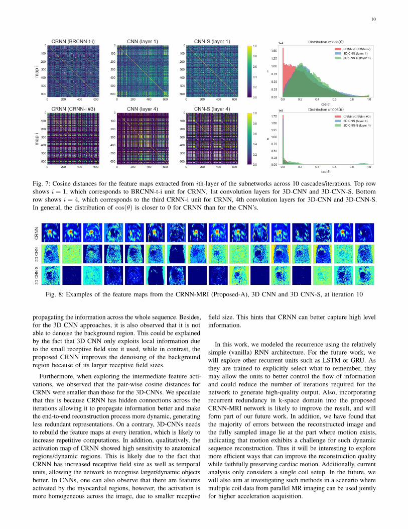
of representations of the subnetworks for i = 1, . . . , 4. Fromone test subject, we extract the feature representations of thesubnetwork across 10 cascades/iterations. By treating eachchannel as a separate feature map, we obtain 640 feature mapsfor each layer i aggregated across iteration. We use the cosinedistance d(A,B) = ATB/‖A‖‖B‖ = cos(θ) to compute thesimilarity between these activation maps for i ∈ 1, 4. If twofeature maps are orthogonal, then cos(θ) = 0 and if two featuremaps are linearly correlated, then cos(θ) = 1. Geometrically,this supports the interpretation that if the cosine distance issmall for all the feature map pairs, then the network is likelyto be capturing diverse patterns. The result is summarised inFig. 7, where the similarity measure is visualised as a matrix,as well as their distributions is plotted for each network.

We can see that for both i ∈ 1, 4, the layers from CRNNappears to have geometrically more orthogonal feature maps.One can also observe that in general, layer 1 has higherredundancy compared to layer 4. In particular, the diagonalyellow stripes can be observed for CNN-S and CRNN, due toparameter-sharing for each cascade. This is not observed in 3D-CNN, even though many features do have high similarity. InFig. 8 we show examples of the feature maps from layer 4 (3rdCRNN-i for CRNN, 4th convolution layers for 3D-CNN and3D-CNN-S) at iteration/cascade 10 of each network during theforward pass. We selected 16 feature maps out of 64 by firstlyclustering them into 16 groups, and then randomly chose onefeature map from each group to show as representative featuremaps in Fig. 8. These feature maps show the activations learnedfrom different networks and is colour-coded (blue correspondsto low activation whereas red corresponds to high activation).We see that CRNN’s features look significantly different fromCNN. In particular, one can observe that some are activatedby the dynamic region, and some are particularly sensitive toregions around the left and/or right ventricle.

V. DISCUSSION

In this work, we have demonstrated that the presentednetwork is capable of producing faithful image reconstructionsfrom highly undersampled data, both in terms of variousquantitative metrics as well as inspection of error maps.In contrast to unrolled deep network architectures proposedpreviously, we modelled the recurrent nature of the optimisationiteration using hidden representations with the ability toretain and propagate information across the optimisation steps.Compared with 3D CNN models, the proposed methods have amuch lower network capacity but still have a higher accuracy,reflecting the effectiveness of our architecture. This is due tothe ability of the proposed RNN units to increase the receptivefield size while iteration steps increase, as well as to efficientlypropagate information across the temporal direction. In fact, foraccelerated imaging, higher undersampling factors significantlyadd aliasing to the initial zero-filled reconstruction, makingthe reconstruction more challenging. This suggests that whilethe 3D CNN possesses higher modelling capacity owing toits large number of parameters, it may not necessarily bean ideal architecture to perform dynamic MR reconstruction,presumably because the simple CNN is not as efficient as

10

Fig. 7: Cosine distances for the feature maps extracted from ith-layer of the subnetworks across 10 cascades/iterations. Top rowshows i = 1, which corresponds to BRCNN-t-i unit for CRNN, 1st convolution layers for 3D-CNN and 3D-CNN-S. Bottomrow shows i = 4, which corresponds to the third CRNN-i unit for CRNN, 4th convolution layers for 3D-CNN and 3D-CNN-S.In general, the distribution of cos(θ) is closer to 0 for CRNN than for the CNN’s.

Fig. 8: Examples of the feature maps from the CRNN-MRI (Proposed-A), 3D CNN and 3D CNN-S, at iteration 10

propagating the information across the whole sequence. Besides,for the 3D CNN approaches, it is also observed that it is notable to denoise the background region. This could be explainedby the fact that 3D CNN only exploits local information dueto the small receptive field size it used, while in contrast, theproposed CRNN improves the denoising of the backgroundregion because of its larger receptive field sizes.

Furthermore, when exploring the intermediate feature acti-vations, we observed that the pair-wise cosine distances forCRNN were smaller than those for the 3D-CNNs. We speculatethat this is because CRNN has hidden connections across theiterations allowing it to propagate information better and makethe end-to-end reconstruction process more dynamic, generatingless redundant representations. On a contrary, 3D-CNNs needsto rebuild the feature maps at every iteration, which is likely toincrease repetitive computations. In addition, qualitatively, theactivation map of CRNN showed high sensitivity to anatomicalregions/dynamic regions. This is likely due to the fact thatCRNN has increased receptive field size as well as temporalunits, allowing the network to recognise larger/dynamic objectsbetter. In CNNs, one can also observe that there are featuresactivated by the myocardial regions, however, the activation ismore homogeneous across the image, due to smaller receptive

field size. This hints that CRNN can better capture high levelinformation.

In this work, we modeled the recurrence using the relativelysimple (vanilla) RNN architecture. For the future work, wewill explore other recurrent units such as LSTM or GRU. Asthey are trained to explicitly select what to remember, theymay allow the units to better control the flow of informationand could reduce the number of iterations required for thenetwork to generate high-quality output. Also, incorporatingrecurrent redundancy in k-space domain into the proposedCRNN-MRI network is likely to improve the result, and willform part of our future work. In addition, we have found thatthe majority of errors between the reconstructed image andthe fully sampled image lie at the part where motion exists,indicating that motion exhibits a challenge for such dynamicsequence reconstruction. Thus it will be interesting to exploremore efficient ways that can improve the reconstruction qualitywhile faithfully preserving cardiac motion. Additionally, currentanalysis only considers a single coil setup. In the future, wewill also aim at investigating such methods in a scenario wheremultiple coil data from parallel MR imaging can be used jointlyfor higher acceleration acquisition.

11

VI. CONCLUSION

Inspired by variable splitting and alternate minimisationstrategies, we have presented an end-to-end deep learningsolution, CRNN-MRI, for accelerated dynamic MRI recon-struction, with a forward, CRNN block implicitly learningiterative denoising interleaved by data consistency layers toenforce data fidelity. In particular, the CRNN architecture iscomposed of the proposed novel variants of convolutionalrecurrent unit which evolves over two dimensions: time anditerations. The proposed network is able to learn both thetemporal dependency and the iterative reconstruction processeffectively, and outperformed the other competing methods interms of both reconstruction accuracy and speed for differentundersampling rates.

REFERENCES

[1] H. Jung, J. C. Ye, and E. Y. Kim, “Improved k–t BLAST and k–t SENSEusing FOCUSS,” Physics in medicine and biology, vol. 52, no. 11, p.3201, 2007.

[2] S. G. Lingala, Y. Hu, E. Dibella, and M. Jacob, “Accelerated dynamicMRI exploiting sparsity and low-rank structure: K-t SLR,” IEEETransactions on Medical Imaging, vol. 30, no. 5, pp. 1042–1054, 2011.

[3] J. Schlemper, J. Caballero, J. V. Hajnal, A. Price, and D. Rueckert, “Adeep cascade of convolutional neural networks for dynamic MR imagereconstruction,” IEEE Transactions on Medical Imaging, vol. 37, no. 2,2018.

[4] D. Batenkov, Y. Romano, and M. Elad, “On the global-local dichotomyin sparsity modeling,” in Compressed Sensing and its Applications.Springer, 2017, pp. 1–53.

[5] J. Tsao, P. Boesiger, and K. P. Pruessmann, “k-t BLAST and k-tSENSE: Dynamic MRI with high frame rate exploiting spatiotemporalcorrelations,” Magnetic Resonance in Medicine, vol. 50, no. 5, pp. 1031–1042, 2003.

[6] J. Caballero, A. N. Price, D. Rueckert, and J. V. Hajnal, “Dictionarylearning and time sparsity for dynamic MR data reconstruction,” IEEETransactions on Medical Imaging, vol. 33, no. 4, pp. 979–994, 2014.

[7] R. Otazo, E. Candès, and D. K. Sodickson, “Low-rank plus sparsematrix decomposition for accelerated dynamic MRI with separation ofbackground and dynamic components,” Magnetic Resonance in Medicine,vol. 73, no. 3, pp. 1125–1136, 2015.

[8] M. Lustig, D. L. Donoho, J. M. Santos, and J. M. Pauly, “Compressedsensing MRI,” IEEE signal processing magazine, vol. 25, no. 2, pp.72–82, 2008.

[9] K. Hammernik, T. Klatzer, E. Kobler, M. P. Recht, D. K. Sodickson,T. Pock, and F. Knoll, “Learning a variational network for reconstructionof accelerated MRI data,” Magnetic resonance in medicine, vol. 79, pp.3055–3071, 2018.

[10] C. Dong, C. C. Loy, K. He, and X. Tang, “Learning a deep convolu-tional network for image super-resolution,” in European Conference onComputer Vision. Springer, 2014, pp. 184–199.

[11] O. Ronneberger, P. Fischer, and T. Brox, “U-net: Convolutional networksfor biomedical image segmentation,” in International Conference onMedical image computing and computer-assisted intervention. Springer,2015, pp. 234–241.

[12] D. Lee, J. Yoo, and J. C. Ye, “Deep artifact learning for compressedsensing and parallel MRI,” arXiv preprint arXiv:1703.01120, 2017.

[13] Y. S. Han, J. Yoo, and J. C. Ye, “Deep learning with domain adap-tation for accelerated projection reconstruction MR,” arXiv preprintarXiv:1703.01135, 2017.

[14] S. Wang, Z. Su, L. Ying, X. Peng, and D. Liang, “Exploiting deepconvolutional neural network for fast magnetic resonance imaging,” inISMRM 24th Annual Meeting and Exhibition, 2016.

[15] S. Wang, N. Huang, T. Zhao, Y. Yang, L. Ying, and D. Liang, “1D PartialFourier Parallel MR imaging with deep convolutional neural network,”in ISMRM 25th Annual Meeting and Exhibition, vol. 47, no. 6, 2017,pp. 2016–2017.

[16] J. Adler and O. Öktem, “Learned primal-dual reconstruction,” IEEETransactions on Medical Imaging, 2018.

[17] J. Sun, H. Li, Z. Xu et al., “Deep ADMM-Net for compressive sensingMRI,” in Advances in Neural Information Processing Systems, 2016, pp.10–18.

[18] J. Schlemper, J. Caballero, J. V. Hajnal, A. Price, and D. Rueckert,“A deep cascade of convolutional neural networks for MR imagereconstruction,” in International Conference on Information Processingin Medical Imaging, 2017, pp. 647–658.

[19] J. Adler and O. Öktem, “Solving ill-posed inverse problems using iterativedeep neural networks,” Inverse Problems, vol. 33, no. 2, p. 124007, 2017.

[20] H. K. Aggarwal, M. P. Mani, and M. Jacob, “MoDL: Model baseddeep learning architecture for inverse problems,” arXiv preprintarXiv:1712.02862, 2017.

[21] M. Mardani, H. Monajemi, V. Papyan, S. Vasanawala, D. Donoho,and J. Pauly, “Recurrent generative adversarial networks for proximallearning and automated compressive image recovery,” arXiv preprintarXiv:1711.10046, 2017.

[22] K. Gregor, I. Danihelka, A. Graves, D. Rezende, and D. Wierstra, “Draw:A recurrent neural network for image generation,” in Proceedings ofThe 32nd International Conference on Machine Learning, 2015, pp.1462–1471.

[23] M. Liang and X. Hu, “Recurrent convolutional neural network for objectrecognition,” in Proceedings of the IEEE Conference on Computer Visionand Pattern Recognition, 2015, pp. 3367–3375.

[24] J. Kuen, Z. Wang, and G. Wang, “Recurrent attentional networks forsaliency detection,” in Proceedings of the IEEE Conference on ComputerVision and Pattern Recognition, 2016, pp. 3668–3677.

[25] Y. Huang, W. Wang, and L. Wang, “Bidirectional recurrent convolutionalnetworks for multi-frame super-resolution,” in Advances in NeuralInformation Processing Systems, 2015, pp. 235–243.

[26] J. L. Elman, “Finding structure in time,” Cognitive science, vol. 14, no. 2,pp. 179–211, 1990.

[27] K. He, X. Zhang, S. Ren, and J. Sun, “Delving deep into rectifiers:Surpassing human-level performance on imagenet classification,” inProceedings of the IEEE international conference on computer vision,2015, pp. 1026–1034.

[28] D. Kingma and J. Ba, “Adam: A method for stochastic optimization,”in The International Conference on Learning Representations (ICLR),2015.

[29] K. P. Pruessmann, M. Weiger, M. B. Scheidegger, P. Boesiger et al.,“SENSE: sensitivity encoding for fast MRI,” Magnetic resonance inmedicine, vol. 42, no. 5, pp. 952–962, 1999.

[30] Z. Wang, A. C. Bovik, H. R. Sheikh, and E. P. Simoncelli, “Imagequality assessment: from error visibility to structural similarity,” IEEEtransactions on image processing, vol. 13, no. 4, pp. 600–612, 2004.

[31] S. Ravishankar and Y. Bresler, “MR image reconstruction from highlyundersampled k-space data by dictionary learning,” IEEE transactionson medical imaging, vol. 30, no. 5, pp. 1028–1041, 2011.

[32] X. Miao, S. G. Lingala, Y. Guo, T. Jao, M. Usman, C. Prieto, and K. S.Nayak, “Accelerated cardiac cine MRI using locally low rank and finitedifference constraints,” Magnetic resonance imaging, vol. 34, no. 6, pp.707–714, 2016.