cooperative coverage based lifetime prolongation for
TRANSCRIPT

Cooperative Coverage Based Lifetime Prolongationfor Microgrid Monitoring WSN in Smart GridSujie Shao ( [email protected] )Lei Wu
Beijing University of Posts and Telecommunications https://orcid.org/0000-0002-2615-1507Qinghang Zhang
Beijing University of Posts and TelecommunicationsNeng Zhang
Beijing University of Posts and TelecommunicationsKaixuan Wang
Shanxi University of Finance and Economics
Research
Keywords: Cooperative coverage, lifetime prolongation, energy consumption, microgrid, improved antcolony optimization
Posted Date: October 21st, 2020
DOI: https://doi.org/10.21203/rs.3.rs-41746/v2
License: This work is licensed under a Creative Commons Attribution 4.0 International License. Read Full License
Version of Record: A version of this preprint was published on December 7th, 2020. See the publishedversion at https://doi.org/10.1186/s13638-020-01857-4.
Cooperative Coverage Based Lifetime Prolongation for Microgrid Monitoring WSN in Smart Grid
Sujie Shao1*, Lei Wu1,Qinghang Zhang1, Neng Zhang1, Kaixuan Wang2
1. Introduction
Due to the growing consumption of energy and natural
resources, distributed renewable energy resources gradually
draw people’s attention [1-2]. To take full advantage of the
flexibility of access and disconnection from the power grid,
organizing distributed renewable energy resources in form of
microgrid as one solution of energy replenishment becomes a
focusing issue in smart grid [3-5]. However, the inherent
randomness and intermittence of energy supplement which are
brought by the changes of status and environment of renewable
energy resources may trouble microgrid operators to realize
effective control and management of the distributed renewable
energy resources, which may have an impact on stability of
smart grid [6]. Therefore, it is necessary to monitor the devices,
networks, resources and environment in the microgrid for
scientific decision-making and efficient operation management.
In order to obtain a large number of accurate and comprehensive
information data about voltage, current, phase angle,
temperature, humidity, frequency and others, a variety of
different corresponding types of sensors need to be deployed [7-
10]. At present, sensors are gradually integrated and
miniaturized, and most of them are battery powered and their
capacity of energy is limited.
For microgrid monitoring business, a variety types of data
are required to work together to complete the relevant data
analysis. The monitoring data like voltage, current, phase angle
of some pivot points of microgrid should be analyzed together
to get the information about power distribution and power loss
for well managing and controlling the usage of renewable
*Correspondence: [email protected]
State Key Laboratory of Networking and Switching Technology,
Beijing University of Posts and Telecommunications, Beijing, China, Full list of
author information is available at the end of the article
energy resources. In addition, temperature, humidity, frequency,
smoke density and other environmental information data should
be analyzed together to detect the probability and type of fault
for quickly and effectively responding fault and well
maintaining the microgrid. Different monitoring business are
organized according to the requirements of different target point.
Different sensors cooperate to be responsible for monitoring
businesses. Therefore, the traditional coverage method can’t well meet the different monitoring requirements of different
target points in the microgrid. Moreover, energy consumption
minimization and lifetime prolongation of the wireless sensor
network (WSN) is another major problem when a huge and
comprehensive data are required according to the different
monitoring requirements.
To solve the problem, WSN for microgrid monitoring may
not be organized according to the type of sensor again, but
organized according to the type of monitoring business, which
means all types of sensors involved by one single monitoring
business should cooperate with each other to complete the
monitoring business. These different types of sensors form a
cooperative coverage set. The number of sensors in the
cooperative coverage set is as small as possible, but only if the
requirement of data collection has been achieved. The reduction
of the number of sensors may destroy the connectivity of the
network, but the coverage set can complete data forwarding
through the cooperation between different types of sensors.
Obviously, more comprehensive raw data will be acquired for
one single monitoring business based on cooperation of different
types of sensors. So the corresponding decision-making of
microgrid operation center may be more conveniently made, and
effectiveness and efficiency of the monitoring business may
consequently get great improvement. In addition, it means more
Abstract To take full advantage of the flexibility of access and disconnection from smart grid, organizing distributed renewable energy
resources in form of microgrid becomes one solution of energy replenishment in smart grid. A large amount of accurate and
comprehensive information data are needed to be monitored by a variety of different types of sensors to guarantee the effective
operation of this kind of microgrid. Energy consumption of microgrid monitoring WSN consequently becomes an issue. This
paper presents a novel lifetime prolongation algorithm based on cooperative coverage of different types of sensors. Firstly,
according to the requirements of monitoring business, the construction of cooperative coverage sets and connected monitoring
WSN are discussed. Secondly, energy consumption is analyzed based on cooperative coverage. Finally, the cooperative
coverage based lifetime prolongation algorithm (CC-LP) is proposed. Both the energy consumption balancing inside the
cooperative coverage set and the switching scheduling between cooperative coverage sets are discussed. Then we draw into an
improved ant colony optimization algorithm to calculate the switching scheduling. Simulation results show that this novel
algorithm can effectively prolong the lifetime of monitoring WSN, especially in the monitoring area with a large deployed
density of different types of sensors.
Keywords:Cooperative coverage, lifetime prolongation, energy consumption, microgrid, improved ant colony optimization
:

page 2 of 12
potential choices of data forwarding for one single sensor and
more reasonable communication process for monitoring WSN.
Moreover, energy consumption control of monitoring WSN has
more possibility for improvement.
Based on the above analysis about sensors cooperation in
microgrid monitoring, we mainly study the following problems
in this paper: 1) How to construct connected monitoring WSN
based on cooperation of different types of sensors to meet the
monitoring requirements in microgrid. 2) How to prolong the
lifetime of WSN based on cooperation of different types of
sensors.
To solve the two problems, the main points are the coverage
of all monitoring target points and the energy consumption of
sensors. A generalized reservation coverage scheduling
algorithm is proposed in the literature [11]. It divides the whole
WSN into several sensor sets, and each set can meet the general
coverage requirement and work in turns to prolong the lifetime
of WSN by scheduling these sets. Liu et al. [12] proposes a
quasi-grid based cooperative coverage algorithm to reduce the
number of active nodes and prolong the lifetime. Bao [13]
prolong the lifetime of WSNs by balancing the energy
consumption inside the group of sensors and scheduling the
working time among different groups of sensors. These
literatures all aimed to reduce the number of sensors working at
the same time while guaranteeing coverage, which can
effectively prolong the lifetime of WSN, but they did not
consider the cooperation of different types of sensors for
multiple types of monitoring businesses. The k-coverage
methods are analyzed in literature [14-15], this deployment and
working mechanism of sensors explains the redundant coverage
of sensors for guaranteeing the quality of monitoring data and
indicates more possibility of coverage and energy consumption
scheduling for monitoring WSNs. Song et al. [16] proposes a
coverage-aware unequal clustering protocol with load separation
for ambient assisted living applications based on WSNs to
achieve better performance and balance energy consumption for
prolonging network lifetime. The above literatures mainly focus
on the coverage performance of monitoring target while
balancing energy consumption and ensuring the quality of data.
However, the cooperation of different types of sensors is not
considered. Xu et al. [17] widely discusses the energy
consumption saving on the privacy-preserving data aggregation
in WSNs by reducing communication overhead and energy
expenditure of sensors. Li et al. [18] proposes a data
compression algorithm to enhance the lifetime of sensors in sea
route monitoring system. Cao [19] divides working time of
sensors into some short time periods and achieves lifetime
prolongation by scheduling these working time periods. These
works save the energy from the perspective of communication
and data. They are very valuable to our work. Afshari et al. [20]
proposes a cooperative fault-tolerant control (CFTC) algorithm
to address the problem of multiple actuator faults in autonomous
AC microgrids. Two new distributed fault tolerant control
algorithms for the restoration of voltage and frequency in
autonomous inverter-interfaced AC microgrids are proposed in
the literature [21]. Dehkordi et al. [22] proposes a novel
distributed noise-resilient secondary control for voltage and
frequency restoration of islanded microgrid inverter-based
distributed generations (DGs) with an additive type of noise.
Raeispour [23] proposes a distributed cooperative control
protocol for inverter-based islanded microgrids. These works
expand more application scenarios of the cooperation of sensors,
including troubleshooting, distributed control, etc. Although all
of the above research does not involve the cooperation of
different types of sensors, the effective methods and ideas
should be used as references. Therefore, cooperation mechanism of different types of
sensors for microgrid monitoring is introduced in this paper. The
cooperative coverage set is firstly discussed to construct the
connected monitoring WSN. Different types of sensors
cooperate to form coverage sets. These coverage sets work in
turns, that can reduce the number of sensors working at the same
time while meeting the coverage rate. Secondly, cooperative
coverage based lifetime prolongation algorithm for microgrid
monitoring WSN is proposed. Energy balance inside the
cooperative coverage sets and switch scheduling between the
cooperative coverage sets are included. Finally, in order to
calculate the switch scheduling, we draw into an improved ant
colony optimization algorithm. Our main contributions are as
follows.
(1) A cooperative coverage based WSN for microgird
monitoring is proposed. In our model, sensors of one
cooperative coverage set are simultaneously in work state to
complete the monitoring business. We constructed cooperative
coverage based microgrid monitoring WSN to connecting a
group of cooperative coverage sets that can combine to cover all
the target points of the monitoring business with some
communication sensors by applying the hierarchical clustering
method. The number of sensors working at the same time keeps
as small as possible to avoid wasting energy while ensuring data
quality.
(2) A cooperative coverage based lifetime prolongation
algorithm for microgrid monitoring WSN is proposed. What’s more, we introduced an improved ant colony optimization
algorithm to calculate the best cooperative coverage set switch
sequence. Simulation results show that this novel algorithm can
effective prolong the lifetime of monitoring WSN with high time
efficiency, especially in the monitoring area with large deployed
density of different types of sensors. The numerical results
verify the practicability and superiority of out algorithm,
comparaed with several other policies.
The rest of this paper is organized as follows. In Section 2,
cooperative coverage based WSN for microgrid monitoring is
introduced. In Section 3, cooperative coverage set of different
types of sensors is studied. The cooperative coverage based
lifetime prolongation (CC-LP) algorithm for microgrid
monitoring WSN is proposed in Section 4. Simulation results are
analyzed in section 5. Section 6 draws the conclusion.
2. Methods In this section, the cooperative coverage based WSN for
distributed renewable energy resources oriented microgrid
monitoring is discussed. According to the requirements of
monitoring business, different types of sensors are organized.
page 3 of 12
They cooperate with each other to complete the corresponding
monitoring tasks.
2.1 Network Structure
The distributed renewable energy resources oriented microgrid
monitoring WSN based on cooperative coverage mainly involves
charging stations, solar devices, wind turbines, energy storage
devices, microgrid operation data center and different
corresponding types of sensors. For the device status, microgrid
operators utilize voltage, current and phase sensors to monitor
the operating status and load information of these distributed
power devices in real time. Meanwhile, different types of
sensors are deployed for specific devices, for example, wind
speed sensor and direction sensor are used to evaluate the
operating status of the wind turbine; light sensor and the
temperature sensor are deployed to collect light and temperature
data around the solar station. For environmental
information,smoke sensors, temperature and humidity sensors
and others need to be deployed to obtain a large number of
accurate and comprehensive information data. In general, these
sensors are mainly used to monitor the status information of the
relevant devices and environmental information, such as voltage,
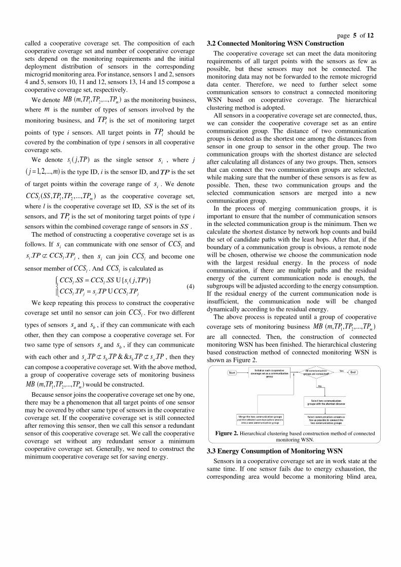
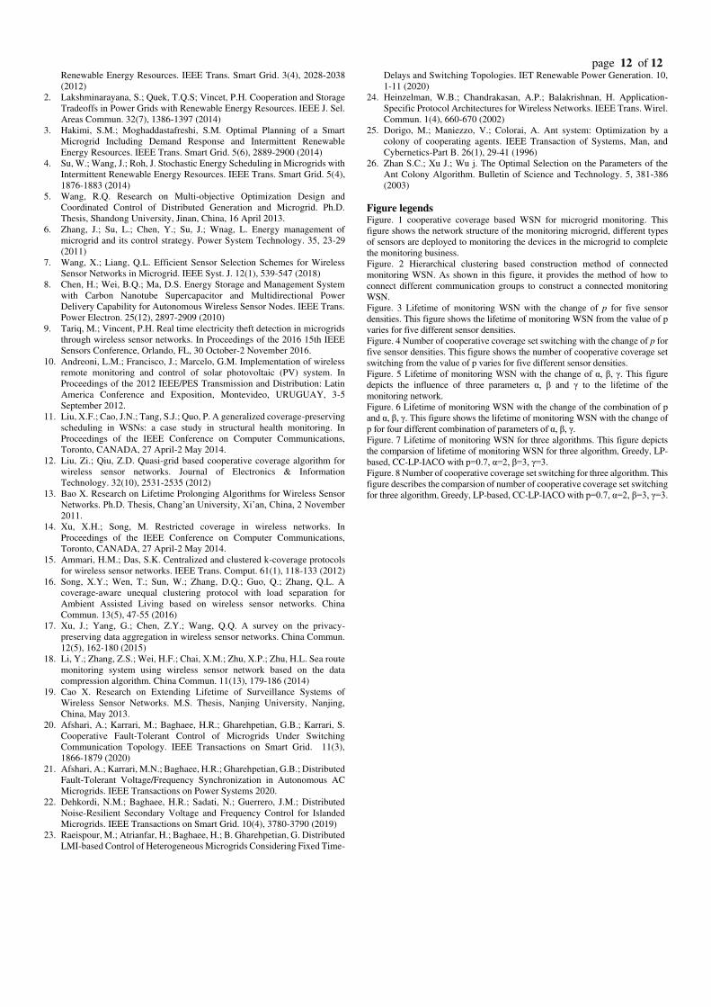
current, phase angle, temperature, humidity, frequency, and so on. As is shown in Figure 1, different types of sensors are
deployed to monitoring the devices in the microgrid to complete
the monitoring business according to the corresponding
requirements. Each type of sensor covers a fixed size monitoring
area which is expressed by the corresponding circle with
different type of dotted line.
The deployment of sensors needs to consider not only the
Euclidean distance between the device and the sensor, but also
the electrical topology of the device. If there are bifurcations on
electrical wires, the phase in every branch need to be acquired.
In order to ensure comprehensiveness of the collected data and
fault tolerance in the monitoring network, we adopted a
redundant deployment scheme. In this scheme, redundant
sensors guarantee that the phase of each branch can be
monitored based on the electrical topology. Monitoring data can
be sent to the access point and data center by data cooperative
communications among different types of sensors.
Each sensor covers at least one monitoring target point. Each
monitoring target point may be covered by at least one sensor
because of the existing of different types of sensors. It is feasible
to select part of sensors in the monitoring area to complete the
monitoring business. Thus, it is unnecessary for every sensor to
be in work state, which indicates the possibility of pursuing
energy consumption minimization and lifetime prolongation
while the monitoring business is ensured.
o
n
m
l
j
i
h
e
c
d
ba
11
15
14 12
10
9
76
4
solar device
charging station
wind turbine
energy storage device
data center
access point
type A type B type C
1
2
3
5
8
13
f
g
k
Fig. 1 cooperative coverage based WSN for microgrid monitoring.
2.2 Cooperative Coverage
In the microgrid monitoring WSN, cooperative coverage of
varied types of sensors mainly contains two meanings. First one
is cooperative coverage with regard to monitoring target points,
which is the cooperation between sensors with the same type.
We call it the first type of cooperative coverage. The other one
is cooperative coverage with regard to data communication,
which is the cooperation between sensors with the different
types. We call it the second type of cooperative coverage.
In order to guarantee the data integrity of monitoring business,
at least one sensor is needed to be deployed for each monitoring
target point to monitor its data change in principle. Each single
sensor has a clear monitoring coverage range. If one monitoring
target point is covered by at last two sensors with the same type
at the same time, activating one of these sensors is theoretically
enough to complete the data acquisition of this monitoring target
point. Thus, sensors with the same type can cooperate together
and select sensors as few as possible to complete monitoring
tasks according to the monitoring requirements, which we call
the first type of cooperative coverage.
We denote ( , )i jr s p as the distance between sensor is and
monitoring target point jp . Generally, the signal strength of
sensor decreases as the ( , )i jr s p increases. To guarantee the
quality of monitoring data, we denote 0r as the threshold of
( , )i jr s p , which means monitoring data of sensor is about
target point jp is valid if 0( , )i j
r s p r . For instance,
monitoring target point i (a charging station) is covered by two
sensors with the same type 8 and 9 at the same time in Figure 1.
Then sensors 8 and 9 can cooperate with each other. From the
perspective of monitoring task of target point i, only one of the
two sensors needs to be in work state.
The first type of cooperative coverage will obviously reduce
the number of single type of sensors that needs to be activated.
However, it may destroy the connectivity of the initial
deployment network, so that parts of sensors may be in an
isolated state. It is necessary to select some other types of sensors
to complete the data forwarding based on the first type of
page 4 of 12
cooperative coverage. Thus, the second type of cooperative
coverage is needed.
If different types of sensors can cooperate and communicate
with each other as long as they are within their communication
range. Then, it is unnecessary to consider the connectivity and
activate other sensors with the same type to complete the data
forwarding during the decision-making process of the first type
of cooperative coverage. Once there is another type of sensor
selected according to the first type of cooperative coverage
within the communication range, the data forwarding can be
completed. Therefore, the connectivity and communication of
monitoring WSN is completed via the cooperation of different
types of sensors, which we call the second type of cooperative
coverage.
The number of activated sensors of whole monitoring WSN
is reduced, resulting in saving unnecessary consumed energy of
sensors. For instance, sensor 2 can forward data of sensor 1 to
the data center, and it is not necessary to activate other type C
sensors as long as sensor 2 has enough energy. Obviously,
sensor 2 must be activated according to the requirements of
monitoring business. The number of activated sensors is reduced.
With the two types of cooperative coverage, sensors which
are in the working state can be divided into three categories:
sensors that only undertake communication tasks, sensors that
only undertake monitoring tasks and sensors that undertake both
of communication and monitoring tasks. We call them
communication sensor, monitoring sensor and dual-function
sensor, respectively. In Figure 1, sensors 2, 4, 5, 8, 10, 12, 13
and 14 are the dual-function sensors. Sensors 1, 7, 9, 11 and 15
are the monitoring sensors. Sensors 3 and 6 are the
communication sensors. Obviously, communication sensors
only play the role of connecting the other sensors to form a
connected monitoring WSN. The monitoring data are sensed by
the monitoring sensors and dual-function sensors, both of them
can cover all the monitoring target points. The three types of
sensor roles may be mutually transformed over time because the
sensor selection will change as the energy consumption of
sensors change over time.
2.3 Energy Consumption of Single Sensor
The working sensor needs to monitor the status of target point
and communicate with other sensors in WSN. Since energy
consumption of sensing data is much smaller than energy
consumption of communications, only energy consumption of
communications is considered in this paper. Energy
consumption of communications can be divided into energy
consumption of receiving data and energy consumption of
transmitting data. According to the first-order wireless
communication energy consumption model, we calculate the
energy consumption of receiving one monitoring data and
energy consumption of transmitting one monitoring data as
, t rd amp r rde e e e e= + = , respectively. rde is energy consumed
by radio devices, ampe is energy consumed by power amplifier,
which is related to the communication distance between two
sensors. For receiving data and transmitting data, rde is same.
We denote k and 0k as the number of monitoring data
received by one single sensor and the number of monitoring data
sensed by one single sensor during one time period, respectively.
Thus, from the perspective of cooperative coverage, energy
consumption of dual-function sensor is in time period t is
calculated as
, 0 0
0 0
( ) ( ) ( )
(2 ) ( )
i t r t rd rd amp
rd amp
e k e k k e k e k k e e
k k e k k e
= + + = + + +
= + + + (1)
Similarly, energy consumption of communication sensor and
that of monitoring sensor in time period t are respectively
calculated as
, 2i t r t rd amp
e k e k e k e k e= + = + (2)
, 0 0 0i t t rd ampe k e k e k e= = + (3)
Then, we can calculate energy consumption of sensors, and
select appropriate sensors to be activated and organized for the
lifetime prolongation of monitoring WSN.
2.4 Communication technologise
In the cooperative coverage based microgrid monitoring
WSN, sensors communicate among themselves and the access
points. The access points communicate with the remote data
processing and control center which store monitoring data and
send control messages. We mainly use ZigBee technology to
enable communication among sensors, as it is widely used in
low-power networks. In addition, most types of sensors, which
are available in smart grid monitoring market, use ZigBee for
communication. ZigBee and other short-range radio
technologies are supported by sensors communicating with
access points. The access points send monitoring data to the
remote data processing and control center through WLAN,
wireless cellular network or high-speed wired network
technologies. Similarly, control messages are forwarded to the
corresponding sensors by access points.
Due to the changing energy consumption of different roles of
sensors and the different business requirements, we need to
select appropriate sensors to construct connected microgrid
monitoring WSN, so that the effective cooperative coverage can
be actually realized. In next section, the cooperative coverage set
is discussed, and we adopt it as the basic element to construct
the connected microgrid monitoring WSN based on cooperative
coverage.
3. Construction of Cooperative Coverage Based
Monitoring WSN In this section, the cooperative coverage set is discussed.
Sensors of one cooperative coverage set are simultaneously in
work state to complete the monitoring business. Then,
cooperative coverage based microgrid monitoring WSN is
constructed by connecting a group of cooperative coverage sets
that can combine to cover all the target points of the monitoring
business with some communication sensors.
3.1 Coverage Cooperative Set
At a specific moment, the cooperative coverage based
monitoring WSN will be split into several disconnected groups
if we remove all communication sensors, and each group can be
page 5 of 12
called a cooperative coverage set. The composition of each
cooperative coverage set and number of cooperative coverage
sets depend on the monitoring requirements and the initial
deployment distribution of sensors in the corresponding
microgrid monitoring area. For instance, sensors 1 and 2, sensors
4 and 5, sensors 10, 11 and 12, sensors 13, 14 and 15 compose a
cooperative coverage set, respectively.
We denote 1 2 ( , , ,..., )m
MB m TP TP TP as the monitoring business,
where m is the number of types of sensors involved by the
monitoring business, and iTP is the set of monitoring target
points of type i sensors. All target points in iTP should be
covered by the combination of type i sensors in all cooperative
coverage sets.
We denote ( , )i
s j TP as the single sensor is , where j
( 1,2,..., )j m= is the type ID, i is the sensor ID, andTP is the set
of target points within the coverage range of is . We denote
1 2( , , ,..., )l m
CCS SS TP TP TP as the cooperative coverage set,
where l is the cooperative coverage set ID, SS is the set of its
sensors, and iTP is the set of monitoring target points of type i
sensors within the combined coverage range of sensors in SS .
The method of constructing a cooperative coverage set is as
follows. If is can communicate with one sensor of l
CCS and
. .i l js TP CCS TP , then is can join l
CCS and become one
sensor member of lCCS . And l
CCS is calculated as
. . { ( , )}
. . .
l l i
l j i l j
CCS SS CCS SS s j TP
CCS TP s TP CCS TP
= =
U
U (4)
We keep repeating this process to construct the cooperative
coverage set until no sensor can join lCCS . For two different
types of sensors as and b
s , if they can communicate with each
other, then they can compose a cooperative coverage set. For
two same type of sensors as and b
s , if they can communicate
with each other and . . & & . .a b b a
s TP s TP s TP s TP , then they
can compose a cooperative coverage set. With the above method,
a group of cooperative coverage sets of monitoring business
1 2 ( , , ,..., )m
MB m TP TP TP would be constructed.
Because sensor joins the cooperative coverage set one by one,
there may be a phenomenon that all target points of one sensor
may be covered by other same type of sensors in the cooperative
coverage set. If the cooperative coverage set is still connected
after removing this sensor, then we call this sensor a redundant
sensor of this cooperative coverage set. We call the cooperative
coverage set without any redundant sensor a minimum
cooperative coverage set. Generally, we need to construct the
minimum cooperative coverage set for saving energy.
3.2 Connected Monitoring WSN Construction
The cooperative coverage set can meet the data monitoring
requirements of all target points with the sensors as few as
possible, but these sensors may not be connected. The
monitoring data may not be forwarded to the remote microgrid
data center. Therefore, we need to further select some
communication sensors to construct a connected monitoring
WSN based on cooperative coverage. The hierarchical
clustering method is adopted.
All sensors in a cooperative coverage set are connected, thus,
we can consider the cooperative coverage set as an entire
communication group. The distance of two communication
groups is denoted as the shortest one among the distances from
sensor in one group to sensor in the other group. The two
communication groups with the shortest distance are selected
after calculating all distances of any two groups. Then, sensors
that can connect the two communication groups are selected,
while making sure that the number of these sensors is as few as
possible. Then, these two communication groups and the
selected communication sensors are merged into a new
communication group.
In the process of merging communication groups, it is
important to ensure that the number of communication sensors
in the selected communication group is the minimum. Then we
calculate the shortest distance by network hop counts and build
the set of candidate paths with the least hops. After that, if the
boundary of a communication group is obvious, a remote node
will be chosen, otherwise we choose the communication node
with the largest residual energy. In the process of node
communication, if there are multiple paths and the residual
energy of the current communication node is enough, the
subgroups will be adjusted according to the energy consumption.
If the residual energy of the current communication node is
insufficient, the communication node will be changed
dynamically according to the residual energy.
The above process is repeated until a group of cooperative
coverage sets of monitoring business 1 2 ( , , ,..., )m
MB m TP TP TP
are all connected. Then, the construction of connected
monitoring WSN has been finished. The hierarchical clustering
based construction method of connected monitoring WSN is
shown as Figure 2.
Figure 2. Hierarchical clustering based construction method of connected
monitoring WSN.
3.3 Energy Consumption of Monitoring WSN
Sensors in a cooperative coverage set are in work state at the
same time. If one sensor fails due to energy exhaustion, the
corresponding area would become a monitoring blind area,
page 6 of 12
resulting in failure of the entire cooperative coverage set. There
is a Barrel Effect for lifetime of cooperative coverage set.
Therefore, energy consumption is another important factor
except monitoring coverage and connectivity when we construct
the cooperative coverage set.
We assume that the number of monitoring data sensed by one
single sensor during one time period is a fixed value. Then, the
total number of monitoring data sensed by the cooperative
coverage set during one time period is known. We assume that
the communication route within the cooperative coverage set
does not change during one time period. Thus, energy
consumption of each sensor during one time period can be
calculated.
We denote ,i tk as the number of data received by i
s during
time period t, which is the sum of data forwarded by all the
descendants of is in the cooperative coverage set during time
period t. Then, energy consumption of dual-function sensor is
in time period t is calculated as
, , , 0
, , 0
, 0
( )
( ) ( )
(2 ) ( )
i t i t r i t t
i t rd i t rd amp
i t rd amp rd amp
e k e k k e
k e k k e e
k e e k e e
= + +
= + + +
= + + +
(5)
The energy consumption of monitoring sensor is still
calculated according to the formula (3).
We call the sensor that forward data to communication sensor
out of the cooperative coverage set the head sensor. According
to the formula (5), energy consumption of head sensor is the
most. Dual-function sensors near the head sensor have the
relatively more energy consumption. Energy consumption of the
monitoring sensor is the least. Thus, energy consumption of
sensors in cooperative coverage set is closely related to the
communication route of sensors. The more times data are
forwarded, the more energy is consumed by the cooperative
coverage set.
To balance the energy consumption, communication route
inside the cooperative coverage set needs to be adjusted over
time, which mainly involves the head sensor. If the energy of the
whole cooperative coverage set can’t support the monitoring
tasks, another new cooperative coverage set need to be
constructed to replace the current one, which may be called
cooperative coverage set switching. Both of the two ways may
change the selection of communication sensors. The specific
methods of adjusting communication route and switching
cooperative coverage set are discussed in the next section.
Energy consumption of communication sensor during one
time period would keep constant if the cooperative coverage set
that it connected and the direction of data forwarding keep
unchanged. According to the formula (2), it can be easily
calculated. Then, the energy consumption of the current
monitoring WSN can be calculated.
To play the greatest advantage of cooperative coverage set,
we need to prolong its working time as much as possible and
further prolong the lifetime of whole microgrid monitoring
WSN based on cooperative coverage according to the actual
energy consumption. We focus on this issue in the next section.
4. Cooperative Coverage Based Lifetime Prolongation
Algorithm In this section, the CC-LP algorithm is proposed. Both the
energy consumption balancing inside the cooperative coverage
set and the switching scheduling between cooperative coverage
sets are discussed. Then we draw into an improved ant colony
optimization algorithm to calculate the switching scheduling.
4.1 Energy Consumption Balancing inside the Cooperat-
ive Coverage set
Cooperative coverage set reduces the number of sensors that
is simultaneously in work state and makes good use of the
redundant deployment of the different types of sensors, but the
tasks of some key sensors may be inevitably increased, which
may lead to extra energy consumption of these sensors to the
disadvantage of the continuous work of the cooperative
coverage set. Thus, balancing the energy consumption of sensors
inside the cooperative coverage set is needed.
We denote ,i tE as the residual energy of i
s at the beginning
of time period t. There are m sensors in the cooperative coverage
set lCCS . Therefore, the number of time periods l
n that lCCS
can continuously run is calculated as
, ,{1,2, , }min ( )
l i t i ti m
n E e=
= L (6)
According to formula (3) and (5), head sensor and its neighbor
sensors may be the energy bottleneck of lCCS , which depend
on the communication route within lCCS . Thus, to eliminate the
energy bottleneck, we need to adjust the communication route.
For adjusting communication route, there are main two ways.
One is fixing the head sensor and adjusting communication path
from other sensors to the head sensor. The other is changing the
head sensor and optimizing the consequent communication
route. The latter one may need to activate other communication
sensors to guarantee the connectivity of WSN. Here, we only
discuss the changing without activating other communication
sensors. If there are several sensors that can communicate with
the current communication sensor, the one with the most
residual energy among them should be selected as the head
sensor at the beginning of each time period.
Changing a new head sensor lead to the network topology in
the cooperative coverage set being rebuilt. According to the
ZigBee technology, extra routing update messages need to be
sent to rebuild the network, resulting in additional energy
consumption. However, considering the position and
composition of sensors in the cooperative coverage set, the head
sensor may be not change if there are no alternative sensors.
Even if the head sensor changes, on the one hand, the head
sensor was changed only in the cooperative coverage set, thus
messages are mainly delivered by sensors inside the set and there
is no other communication sensor to be activated. On the other
hand, the number of sensors in one cooperative coverage set and
routing update messages is relatively small, so the extra energy
consumption of delivering routing update messages is less than
page 7 of 12
the energy consumption of transmitting monitoring data, and has
a weak effect on the overall performance of our algorithm.
For a given head sensor, the communication route
optimization can be transformed to how to find the maximum
value of minimum residual energy ,i t wE + after w time periods
that lCCS continuously run. The problem can be expressed as
formula (7): 𝐸 = 𝑚𝑎𝑥( 𝑚𝑖𝑛𝑖=1,2,…,𝑚}(𝐸𝑖,𝑡+𝑤)), 𝑤 ∈ [1, 𝑛𝑙] (7)
where E is the energy bottleneck of lCCS .
After one time period, the residual energy of is can be
calculated as
, 1 , ,i t i t i tE E e+ = − (8)
Then, ,i t wE + will be calculated by repeating the formula (8)
w times, and the energy consumption balancing inside the
cooperative coverage set is achieved.
4.2 Switching Scheduling between Cooperative Coverage
Sets
Moreover, when a cooperative coverage set fails due to the
energy exhaustion or it needs to stop working due to the
switching scheduling for lifetime prolongation, a new
cooperative coverage set is needed to be constructed to complete
the monitoring tasks instead. Then, some sensors may need to
be activated from the sleep state and some other sensors need to
sleep again, which inevitably lead to extra energy consumption
of these sensors too. Frequent switching between different
cooperative coverage sets may not necessarily enable the
lifetime prolongation of microgrid monitoring WSN. Therefore,
selecting appropriate cooperative coverage set and switching at
the appropriate time are also needed.
There may be more than one cooperative coverage set that can
complete the monitoring tasks. For reducing the switching times,
we sort all these cooperative coverage sets according to their
minimum residual energy of sensor in descending order. Then
we select the switching candidate cooperative coverage set in
order.
Moreover, one sensor may be selected by different
cooperative coverage sets at different time period. Then its
energy consumption of the previous switching round definitely
affect the working time of the next switching round. Thus, we
set another energy threshold p to determine the appropriate
switching timing of current cooperative coverage set in some
cases, which means the formula (7) may be constrained. We
denote c
iE as the energy capacity of i
s . If ,
c
i t iE pE , we can
consider that is is no longer suitable for continuous working.
When more than half of sensors happen like this, we can
consider that the current cooperative coverage set is no longer
suitable for continuous working if there is another cooperative
coverage set can be switched. However, this constraint is not
necessary because our switching scheduling can still continue if
all of the cooperative coverage sets meet the condition, which
obviously means the lifetime of the monitoring WSN will end
soon.
To simplify the problem, we still use lCCS to denote the
switching cooperative coverage set. Then, the number of time
periods ln that l
CCS can continuously run is calculated as
formula (9):
,0 ,1min( , )l l l
n n n= , (9)
where
,0 , ,{1,2, , }
min ( )l i t i t
i m cn E e
= − = L
, (10)
and
,1 , 0 ,{ 1, 2,..., }
min ( ( ) )l i t i t
i m c m c mn E E e
= − + − + = − (11)
0E is denoted as the energy consumption of activating a sensor,
m and c are total number of sensors in lCCS and number of
sensors that are activated to construct lCCS , respectively.
If 0l
n = , lCCS definitely can’t be the switching candidate
cooperative coverage set. Thus, we can select number from
[1, ]l
n to schedule the work state or sleep state of lCCS .
Assuming that lifetime of monitoring WSN ends after q times
switching of cooperative coverage set, the problem of lifetime
prolongation of monitoring WSN is transformed into how to
select the appropriate number of working time periods of
cooperative coverage sets to prolong the lifetime. The problem
can be expressed as formula (12), where sn is the maximum
lifetime of monitoring WSN, jw is the number of time periods
that lCCS continuously run in the j-th switching.
1
max( ), [1, ]q
j j l
j
sn w w n=
= (12)
For each jw , it derived from the formula (7), and
, ,( 1, 1,..., )i t
E i m c m c m= − + − + in formula (8) is modified as
, 0i tE E− . m and c are the specific ones in the j-th cooperative
coverage set.
4.3 CC-LP Algorithm Based on Improved Ant Colony
Optimization
In this subsection, the CC-LP algorithm based on improved
ant colony optimization is proposed to calculate the best
cooperative coverage set switch sequence. Compared with the
common ant colony optimization algorithm, we have made some
improvements in our algorithm. The improvement schemes of
our algorithm are as follows.
(1) To select the next cooperative coverage set, we propose a
probability formula based on pheromone, residual energy and
switch energy consumption of coverage set.
page 8 of 12
(2) If we use the common ACO algorithm, the same
cooperative coverage set will not be repeatedly selected. But in
our model, when the cooperative coverage set has sufficient
energy, the same cooperative coverage set should be repeatedly
selected to avoid frequent switching and excessive energy
consumption. Therefore, we optimized the pheromone update
method of our improved ant colony optimization algorithm,
expanded the selectable path, and searched for more solution
space.
We denote the number of ants as M and the number of
cooperative coverage sets as n. Each ant has a tabu table that
records the cooperative coverage sets whose residual energy is
not enough, these cooperative coverage sets cannot be selected.
Firstly, we randomly place all ants on cooperative coverage sets,
and assume the pheromone in coverage set is (0)ij ( (0)
ij is a
constant). Secondly, we calculate the probability that ant k
switches from 𝐶𝐶𝑆𝑖 to 𝐶𝐶𝑆𝑗 based on formula (13):
*, j
( ) *
0, j
[ ][ ( )] [ ]
[ ][ ( )] [ ]k
k
ijs
k
jij ij
tsis is
Tabu
t LTabu
tP L
Tabu
=
(13)
In formula (13), k is the ID of ants and 𝑇𝑎𝑏𝑢𝑘 is the tabu
table of ant k. We denote ij as the pheromone of 𝐶𝐶𝑆𝑖 to 𝐶𝐶𝑆𝑗.
Furthermore, jL is the residual energy, and formula (12)
describes the calculation of jL :
, ,, ,{1,2, , }
( / ) / min( / )j i t i ti t i t
i m
me eL E E=
= + (14)
In formula (14), jL obtained by adding the average and
minimum values of the remaining time periods of all nodes in
cooperative coverage set j.
We denote ij as the heuristic information of 𝐶𝐶𝑆𝑖 to𝐶𝐶𝑆𝑗 .
Formula (13) describes the calculation of ij :
1
( ),
j
ijact i
s
s s
ccsccsE
=
(15)
In formula (15), we denote 𝐸𝑎𝑐𝑡(𝑠) as the additional energy
consumption of node s. If node s in 𝐶𝐶𝑆𝑗 not be included in 𝐶𝐶𝑆𝑖, additional energy consumption 𝐸𝑎𝑐𝑡(𝑠) will be calculated in this
formula.
What’s more, in formula (13), α is a heuristic factor, which
reflects the relative importance of pheromone. The larger α is,
the more likely the ants are to select the previous path, and the
less the randomness of the ant colony search. β and γ
respectively reflect the relative importance of residual energy
and switch energy consumption when an ant selects next
cooperative coverage set. The larger β and γ is, the more likely
the ants fall into the local optimum.
These three parameters are very important parameters in the
algorithm, and the selection method will affect global
convergence and calculating efficiency of the ant colony
algorithm. Meanwhile, functions of the parameters in the ant
colony algorithm are closely related. If these parameters are not
configured properly, the solution speed will be very slow and the
lifetime of network will be dissatisfied.
After all ants select the coverage set through formula (13) and
run to the end, we only perform global pheromone update on the
best path. On the one hand, it allows the ants to find a better path
based on the residual concentration of pheromone on the path.
On the other hand, it allows the ants to search for optimal
solution at a faster speed and promotes the convergence of the
algorithm. In our model, in order to maximize the lifetime of a
network, the network may select 𝐶𝐶𝑆𝑖 until the energy
consumption of 𝐶𝐶𝑆𝑖 reaches the threshold. Formula (16) and
formula (17) describe the update method of global pheromone:
/ , ( )
/( * ),
best
ij
best i
Q i jt
Q i j
L
CL
= =
(16)
( 1) (1 ) ( ) * ( )ij ij ij
t t RHQ t + = − +
(17)
In formula (16) and formula (17), we denote Q as the sum of
pheromone for an ant. 𝐿𝑏𝑒𝑠𝑡 is the length of the best path and
RHQ is the attenuation rate of pheromone. ρ represents the
pheromone volatilization rate, and ρ has an impact on the search ability and convergence speed of our algorithm. We denote Ci as
the number of select the same 𝐶𝐶𝑆𝑖 continuously. Obviously, as Ci increases, the average energy of CCSi will gradually decrease.
When an ant selects the same 𝐶𝐶𝑆𝑖 in the next iteration, Ci ensures that the incremental value of pheromone is inversely
proportional to the number of select times. Thus, the energy of
sensors in the monitoring network can be balanced and the
lifetime of monitoring network can be prolonged.
In our algorithm, the number of iteration N is set. In each
iteration, there will be M ants searching the switching path
according formula (13) at the same time. The search process of
each any is the switching sequence of the coverage sets until it
cannot find a set of sensors that can meet the requirements of
monitoring business. When the search process ends, the lifetime
of monitoring WSN also ends. The complexity of the algorithm
is related to the number of cooperative coverage sets constructed.
However, it is hard to obtain an accurate function mapping of
the number of sensors and the number of corresponding
cooperative coverage sets, because the location and number of
sensors in the monitoring WSN are random and network model
is complicated. We assume the number of constructed coverage
sets is C, then the complexity of CC-LP-IACO is 𝑂 =(𝑁 × 𝐶2 × 𝑀). The algorithm is shown in Algorithm 1.
Algorithm 1 Improved ant colony optimization algorithm based
on CC-LP
01: Input: cooperative coverage sets CCS, number of iterator N
02: Output: maximum sensor network lifetime Lmax
03: Initialization parameters(α, β, γ) 04: 𝐿𝑚𝑎𝑥 ← 0, pheromone matrix[][] ← Q
05: while iteration N do
06: for k = 0 → M do
07: Antk lifetime ALk ← 0
08: 𝑇𝑎𝑏𝑢𝑘 ←
09: Randomly select an initial set
page 9 of 12
10: while not all CCS 𝑇𝑎𝑏𝑢𝑘
11: Calculate the probability of each set according
formula (13)
12: Used roulette algorithm to select next set by the
probability
13: for l = 0 → num(CCS) do
14: if the minimum lifetime of sensors in set min(𝐸𝑖,𝑡 /𝑒𝑖,𝑡) ≤ 0 then
15: 𝑇𝑎𝑏𝑢𝑘.append[𝐶𝐶𝑆𝑙] 16: end if
17: 𝐴𝐿𝑘 = 𝐴𝐿𝑘 + 1
18: end for
19: compare 𝐴𝐿𝑘 of each ant to select 𝐴𝑛𝑡𝑏𝑒𝑠𝑡
20: if max(𝐴𝐿𝑘) 𝐿𝑚𝑎𝑥 then
21: 𝐿𝑚𝑎𝑥← max(𝐴𝐿𝑘)
22: end if
23: end while
24: end for
25: for i = 0 → num(CCS) do
26: for j = 0 → num(CCS) do
27: if [i,j] in the path of 𝐴𝑛𝑡𝑏𝑒𝑠𝑡 then
28: update the pheromone[i][j] according formula (16)
29: end if
30: end for
31: end for
32: end while
5 Simulation Results and discussion In this section, the performance of our proposed CC-LP
algorithm is evaluated. There are 3 types of sensors in the
simulated monitoring WSN. Their coverage ranges are 10m,
15m and 20m, respectively. The number of each type of sensors
is same. Each type of sensor needs to monitor 10 target points
that are randomly scattered in 100*100 m2 area. There is one
access point in the center of the area. Our simulation was
programmed by python3.6 and was run on the computer with i5-
7300HQ CPU @ 2.50GHz and 8 GB of RAM.
In this paper, energy consumption of node sending and
receiving data is the same as the energy consumption model of
wireless sensor network in literature [24], which is a first-order
wireless communication model. Each resource node generates a
certain number of data packets in each time period. The size of
the data packet is 100 Byte, and the initial energy of the sensor
node is 0.05J. The parameter settings are shown in Table 1.
Table 1. parameter settings.
Parameter values Unit
Node distribution region 100×100 -
Position of the base station (50, 50) -
The number of nodes 60, 80, 100,
120,150 -
The initial energy of each node 0.05 J
Total size of data 800 bit
rdE 5×10⁻⁸J bit
ampE 1×10-11J bit
In the design of our CC-LP, the value of p is the factor that
will actually affect the performance of lifetime prolongation.
Firstly, 60, 80, 100,120 and 150 sensors are deployed in the area,
and simulations are carried out under these four sensor densities
to determine the optimal value of p. The number of sensors in
real microgrid is much greater than this number, but the
mechanism of cooperative coverage of real microgrid is the
same as our simulation. Secondly, in order to optimize the CC-
LP algorithm, we compare the influence of α, β and γ to the
network and the performance of different number of nodes.
Thirdly, to further evaluate performance of fault detection, we
compare CC-LP with the greedy algorithm and LP-based
heuristic proposed in literature [18]. The greedy algorithm
switches the cooperative coverage that can meet the requirement
of monitor business and own the most residual energy,
regardless of the switch consumption to the next switch round.
LP-based heuristic selects nodes to be added to the coverage set
by transform the selection process to integer programming while
spending a time period. To ensure statistical validity, the data
used in the simulation results analysis are averaged and all
simulation experiments are repeated 100 times.
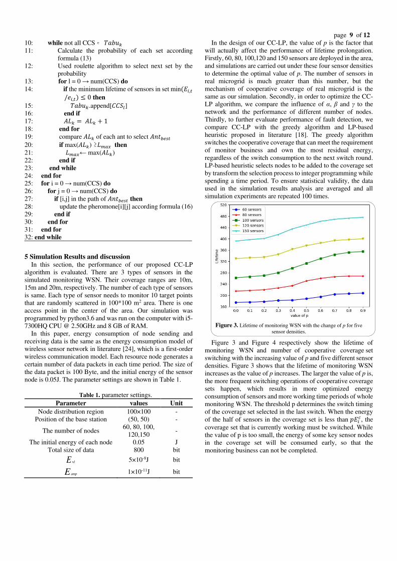
Figure 3. Lifetime of monitoring WSN with the change of p for five
sensor densities.
Figure 3 and Figure 4 respectively show the lifetime of
monitoring WSN and number of cooperative coverage set
switching with the increasing value of p and five different sensor
densities. Figure 3 shows that the lifetime of monitoring WSN
increases as the value of p increases. The larger the value of p is,
the more frequent switching operations of cooperative coverage
sets happen, which results in more optimized energy
consumption of sensors and more working time periods of whole
monitoring WSN. The threshold p determines the switch timing
of the coverage set selected in the last switch. When the energy
of the half of sensors in the coverage set is less than 𝑝𝐸𝑖𝑐, the
coverage set that is currently working must be switched. While
the value of p is too small, the energy of some key sensor nodes
in the coverage set will be consumed early, so that the
monitoring business can not be completed.
page 10 of 12
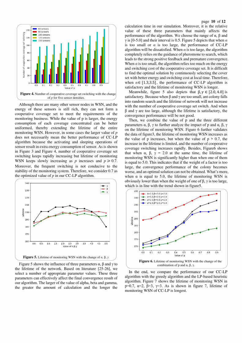
Figure 4. Number of cooperative coverage set switching with the change
of p for five sensor densities.
Although there are many other sensor nodes in WSN, and the
energy of these sensors is still rich, they can not form a
cooperative coverage set to meet the requirements of the
monitoring business. While the value of p is larger, the energy
consumption of each coverage concentrated can be better
uniformed, thereby extending the lifetime of the entire
monitoring WSN. However, in some cases the larger value of p
does not necessarily mean the better performance of CC-LP
algorithm because the activating and sleeping operations of
sensor result in extra energy consumption of sensor. As is shown
in Figure 3 and Figure 4, number of cooperative coverage set
switching keeps rapidly increasing but lifetime of monitoring
WSN keeps slowly increasing as p increases and p≥ 0.7.
Moreover, the frequent switching is not conducive to the
stability of the monitoring system. Therefore, we consider 0.7 as
the optimized value of p in our CC-LP algorithm.
Figure 5. Lifetime of monitoring WSN with the change of α, β, γ.
Figure 5 shows the influence of three parameters α, β and γ to the lifetime of the network. Based on literature [25-26], we
select a number of appropriate parameter values. These three
parameters can effectively affect the final convergence result of
our algorithm. The larger of the value of alpha, beta and gamma,
the greater the amount of calculation and the longer the
calculation time in our simulation. Moreover, it is the relative
value of these three parameters that mainly affects the
performance of the algorithm. We choose the range of α, β and γ is [0-5.0] and their interval is 0.5. Figure 5 depicts that when α
is too small or α is too large, the performance of CC-LP
algorithm will be dissatisfied. When α is too large, the algorithm
completely relies on the guidance of pheromone to search, which
leads to the strong positive feedback and premature convergence.
When α is too small, the algorithm relies too much on the energy
and switching cost of the cooperative coverage set. It is difficult
to find the optimal solution by continuously selecting the cover
set with better energy and switching cost at local time. Therefore,
when α∈ [1.3,3.5] , the performance of CC-LP algorithm is
satisfactory and the lifetime of monitoring WSN is longer.
Meanwhile, figure 5 also depicts that β, 𝛾 ∈ [2.0, 4.0] is
satisfactory. Because when β and γ are too small, ant colony falls into random search and the lifetime of network will not increase
with the number of cooperative coverage set switch. And when
β and γ are too large, although the lifetime is satisfactory, the convergence performance will be not good.
Then, we combine the value of p and the three different
parameters α, β, γ to further analyze the impact of p and α, β, γ on the lifetime of monitoring WSN. Figure 6 further validates
the data of figure3, the lifetime of monitoring WSN increases as
the value of p increases, but when the value of p > 0.7, the
increase in the lifetime is limited, and the number of cooperative
coverage switching increases rapidly. Besides, Figure6 shows
that when α, β, γ = 2.0 at the same time, the lifetime of monitoring WSN is significantly higher than when one of them
is equal to 5.0. This indicates that if the weight of a factor is too
large, the convergence performance of the colony becomes
worse, and an optimal solution can not be obtained. What’s more, when α is equal to 5.0, the lifetime of monitoring WSN is obviously lower than when the weight of one of β, γ is too large, which is in line with the trend shown in figure5.
Figure 6. Lifetime of monitoring WSN with the change of the
combination of p and α, β, γ.
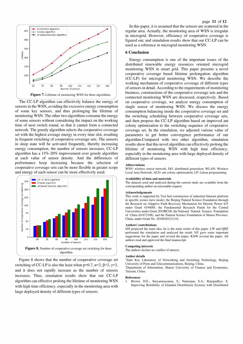
In the end, we compare the performance of our CC-LP
algorithm with the greedy algorithm and the LP-based heuristic
algorithm. Figure 7 shows the lifetime of monitoring WSN in
p=0.7, α=2, β=3, γ=3. As is shown in figure 7, lifetime of
monitoring WSN of CC-LP is longest.
page 11 of 12
Figure 7. Lifetime of monitoring WSN for three algorithms.
The CC-LP algorithm can effectively balance the energy of
sensors in the WSN, avoiding the excessive energy consumption
of some key sensors, and thus prolonging the lifetime of
monitoring WSN. The other two algorithms consume the energy
of some sensors without considering the impact on the working
time of next switch round, so that it cannot form a connected
network. The greedy algorithm selects the cooperative coverage
set with the highest average energy in every time slot, resulting
in frequent switching of cooperative coverage sets. The sensors
in sleep state will be activated frequently, thereby increasing
energy consumption. the number of sensors increases, CC-LP
algorithm has a 15%-20% improvement over greedy algorithm
at each value of sensor density. And the differences of
performance keep increasing because the selection of
cooperative coverage sets can be more flexible in greater scope
and energy of each sensor can be more effectively used.
Figure 8. Number of cooperative coverage set switching for three
algorithm.
Figure 8 shows that the number of cooperative coverage set
switching of CC-LP is also the least when p=0.7, α=2, β=3, γ=3, and it does not rapidly increase as the number of sensors
increases. Thus, simulation results show that our CC-LP
algorithm can effective prolong the lifetime of monitoring WSN
with high time efficiency, especially in the monitoring area with
large deployed density of different types of sensors.
In this paper, it is assumed that the sensors are scattered in the
regular area. Actually, the monitoring area of WSN is irregular
in microgrid. However, efficiency of cooperative coverage is
figured out, and simulation results show that our CC-LP can be
used as a reference in microgrid monitoring WSN.
6 Conclusion
Energy consumption is one of the important issues of the
distributed renewable energy resources oriented microgrid
monitoring WSN in smart grid. This paper presents a novel
cooperative coverage based lifetime prolongation algorithm
(CC-LP) for microgrid monitoring WSN. We describe the
working mechanism of cooperative coverage of different types
of sensors in detail. According to the requirements of monitoring
business, constructions of the cooperative coverage sets and the
connected monitoring WSN are discussed, respectively. Based
on cooperative coverage, we analyze energy consumption of
single sensor of monitoring WSN. We discuss the energy
consumption balancing inside the cooperative coverage set and
the switching scheduling between cooperative coverage sets,
and then propose the CC-LP algorithm based on improved ant
colony optimization to the switching sequence of cooperative
coverage set. In the simulation, we adjusted various value of
parameters to get better convergence performance of our
algorithm.Compared with two other algorithm, simulation
results show that this novel algorithm can effectively prolong the
lifetime of monitoring WSN with high time efficiency,
especially in the monitoring area with large deployed density of
different types of sensors.
Abbreviations
WSN: wireless sensor network; DG: distributed generation; WLAN: Wireless
Local Area Network; ACO: ant colony optimization; LP: Linear programming
Availability of data and materials
The datasets used and analysed during the current study are available from the
corresponding author on reasonable request.
Acknowledgements This work is supported by Test bed construction of industrial Internet platform
in specific scenes (new mode), the Beijing Natural Science Foundation through
the Research on Adaptive Fault Recovery Mechanism for Electric Power IoT
under Grant 4194085, the Fundamental Research Funds for the Central
Universities under Grant 2019RC08, the National Natural Science Foundation
of China (61672108), and the Natural Science Foundation of Shanxi Province,
China, under Grant No. 201801D121116.
Authors’ contributions
SJS proposed the main idea, he is the main writer of this paper. LW and QHZ
performed the simulation and analyzed the result. NZ gave some important
suggestions for the paper and revised the paper, KXW revised the paper. All
authors read and approved the final manuscript.
Competing interests
The authors declare no conflict of interest.
Author details 1State Key Laboratory of Networking and Switching Technology, Beijing University of Posts and Telecommunications, Beijing, China. 2Department of Information, Shanxi University of Finance and Economics, Taiyuan, China.
References
1. Brown, H.E.; Suryanarayanna, S.; Natarajan, S.A.; Rajopadhye, S.
Improving Reliability of Islanded Distribution Systems with Distributed
page 12 of 12 Renewable Energy Resources. IEEE Trans. Smart Grid. 3(4), 2028-2038
(2012)
2. Lakshminarayana, S.; Quek, T.Q.S; Vincet, P.H. Cooperation and Storage
Tradeoffs in Power Grids with Renewable Energy Resources. IEEE J. Sel.
Areas Commun. 32(7), 1386-1397 (2014)
3. Hakimi, S.M.; Moghaddastafreshi, S.M. Optimal Planning of a Smart
Microgrid Including Demand Response and Intermittent Renewable
Energy Resources. IEEE Trans. Smart Grid. 5(6), 2889-2900 (2014)
4. Su, W.; Wang, J.; Roh, J. Stochastic Energy Scheduling in Microgrids with
Intermittent Renewable Energy Resources. IEEE Trans. Smart Grid. 5(4),
1876-1883 (2014)
5. Wang, R.Q. Research on Multi-objective Optimization Design and
Coordinated Control of Distributed Generation and Microgrid. Ph.D.
Thesis, Shandong University, Jinan, China, 16 April 2013.
6. Zhang, J.; Su, L.; Chen, Y.; Su, J.; Wnag, L. Energy management of
microgrid and its control strategy. Power System Technology. 35, 23-29
(2011)
7. Wang, X.; Liang, Q.L. Efficient Sensor Selection Schemes for Wireless
Sensor Networks in Microgrid. IEEE Syst. J. 12(1), 539-547 (2018)
8. Chen, H.; Wei, B.Q.; Ma, D.S. Energy Storage and Management System
with Carbon Nanotube Supercapacitor and Multidirectional Power
Delivery Capability for Autonomous Wireless Sensor Nodes. IEEE Trans.
Power Electron. 25(12), 2897-2909 (2010)
9. Tariq, M.; Vincent, P.H. Real time electricity theft detection in microgrids
through wireless sensor networks. In Proceedings of the 2016 15th IEEE
Sensors Conference, Orlando, FL, 30 October-2 November 2016.
10. Andreoni, L.M.; Francisco, J.; Marcelo, G.M. Implementation of wireless
remote monitoring and control of solar photovoltaic (PV) system. In
Proceedings of the 2012 IEEE/PES Transmission and Distribution: Latin
America Conference and Exposition, Montevideo, URUGUAY, 3-5
September 2012.
11. Liu, X.F.; Cao, J.N.; Tang, S.J.; Quo, P. A generalized coverage-preserving
scheduling in WSNs: a case study in structural health monitoring. In
Proceedings of the IEEE Conference on Computer Communications,
Toronto, CANADA, 27 April-2 May 2014.
12. Liu, Zi.; Qiu, Z.D. Quasi-grid based cooperative coverage algorithm for
wireless sensor networks. Journal of Electronics & Information
Technology. 32(10), 2531-2535 (2012)
13. Bao X. Research on Lifetime Prolonging Algorithms for Wireless Sensor
Networks. Ph.D. Thesis, Chang’an University, Xi’an, China, 2 November 2011.
14. Xu, X.H.; Song, M. Restricted coverage in wireless networks. In
Proceedings of the IEEE Conference on Computer Communications,
Toronto, CANADA, 27 April-2 May 2014.
15. Ammari, H.M.; Das, S.K. Centralized and clustered k-coverage protocols
for wireless sensor networks. IEEE Trans. Comput. 61(1), 118-133 (2012)
16. Song, X.Y.; Wen, T.; Sun, W.; Zhang, D.Q.; Guo, Q.; Zhang, Q.L. A
coverage-aware unequal clustering protocol with load separation for
Ambient Assisted Living based on wireless sensor networks. China
Commun. 13(5), 47-55 (2016)
17. Xu, J.; Yang, G.; Chen, Z.Y.; Wang, Q.Q. A survey on the privacy-
preserving data aggregation in wireless sensor networks. China Commun.
12(5), 162-180 (2015)
18. Li, Y.; Zhang, Z.S.; Wei, H.F.; Chai, X.M.; Zhu, X.P.; Zhu, H.L. Sea route
monitoring system using wireless sensor network based on the data
compression algorithm. China Commun. 11(13), 179-186 (2014)
19. Cao X. Research on Extending Lifetime of Surveillance Systems of
Wireless Sensor Networks. M.S. Thesis, Nanjing University, Nanjing,
China, May 2013.
20. Afshari, A.; Karrari, M.; Baghaee, H.R.; Gharehpetian, G.B.; Karrari, S.
Cooperative Fault-Tolerant Control of Microgrids Under Switching
Communication Topology. IEEE Transactions on Smart Grid. 11(3),
1866-1879 (2020)
21. Afshari, A.; Karrari, M.N.; Baghaee, H.R.; Gharehpetian, G.B.; Distributed
Fault-Tolerant Voltage/Frequency Synchronization in Autonomous AC
Microgrids. IEEE Transactions on Power Systems 2020.
22. Dehkordi, N.M.; Baghaee, H.R.; Sadati, N.; Guerrero, J.M.; Distributed
Noise-Resilient Secondary Voltage and Frequency Control for Islanded
Microgrids. IEEE Transactions on Smart Grid. 10(4), 3780-3790 (2019)
23. Raeispour, M.; Atrianfar, H.; Baghaee, H.; B. Gharehpetian, G. Distributed
LMI-based Control of Heterogeneous Microgrids Considering Fixed Time-
Delays and Switching Topologies. IET Renewable Power Generation. 10,
1-11 (2020)
24. Heinzelman, W.B.; Chandrakasan, A.P.; Balakrishnan, H. Application-
Specific Protocol Architectures for Wireless Networks. IEEE Trans. Wirel.
Commun. 1(4), 660-670 (2002)
25. Dorigo, M.; Maniezzo, V.; Colorai, A. Ant system: Optimization by a
colony of cooperating agents. IEEE Transaction of Systems, Man, and
Cybernetics-Part B. 26(1), 29-41 (1996)
26. Zhan S.C.; Xu J.; Wu j. The Optimal Selection on the Parameters of the
Ant Colony Algorithm. Bulletin of Science and Technology. 5, 381-386
(2003)
Figure legends Figure. 1 cooperative coverage based WSN for microgrid monitoring. This
figure shows the network structure of the monitoring microgrid, different types
of sensors are deployed to monitoring the devices in the microgrid to complete
the monitoring business.
Figure. 2 Hierarchical clustering based construction method of connected
monitoring WSN. As shown in this figure, it provides the method of how to
connect different communication groups to construct a connected monitoring
WSN.
Figure. 3 Lifetime of monitoring WSN with the change of p for five sensor
densities. This figure shows the lifetime of monitoring WSN from the value of p
varies for five different sensor densities.
Figure. 4 Number of cooperative coverage set switching with the change of p for
five sensor densities. This figure shows the number of cooperative coverage set
switching from the value of p varies for five different sensor densities.
Figure. 5 Lifetime of monitoring WSN with the change of α, β, γ. This figure depicts the influence of three parameters α, β and γ to the lifetime of the monitoring network.
Figure. 6 Lifetime of monitoring WSN with the change of the combination of p
and α, β, γ. This figure shows the lifetime of monitoring WSN with the change of
p for four different combination of parameters of α, β, γ. Figure. 7 Lifetime of monitoring WSN for three algorithms. This figure depicts
the comparsion of lifetime of monitoring WSN for three algorithm, Greedy, LP-
based, CC-LP-IACO with p=0.7, α=2, β=3, γ=3. Figure. 8 Number of cooperative coverage set switching for three algorithm. This
figure describes the comparsion of number of cooperative coverage set switching
for three algorithm, Greedy, LP-based, CC-LP-IACO with p=0.7, α=2, β=3, γ=3.
Figures
Figure 1
cooperative coverage based WSN for microgrid monitoring.
Figure 2
Hierarchical clustering based construction method of connected monitoring WSN.
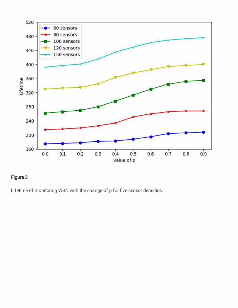
Figure 3
Lifetime of monitoring WSN with the change of p for �ve sensor densities.
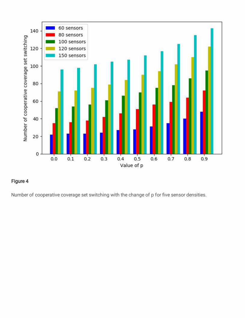
Figure 4
Number of cooperative coverage set switching with the change of p for �ve sensor densities.
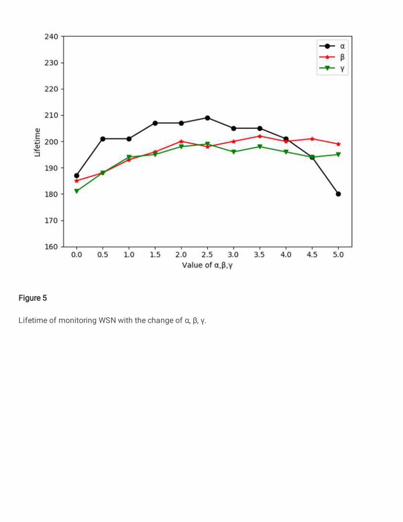
Figure 5
Lifetime of monitoring WSN with the change of α, β, γ.
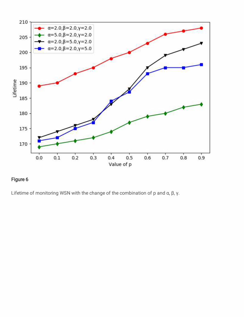
Figure 6
Lifetime of monitoring WSN with the change of the combination of p and α, β, γ.
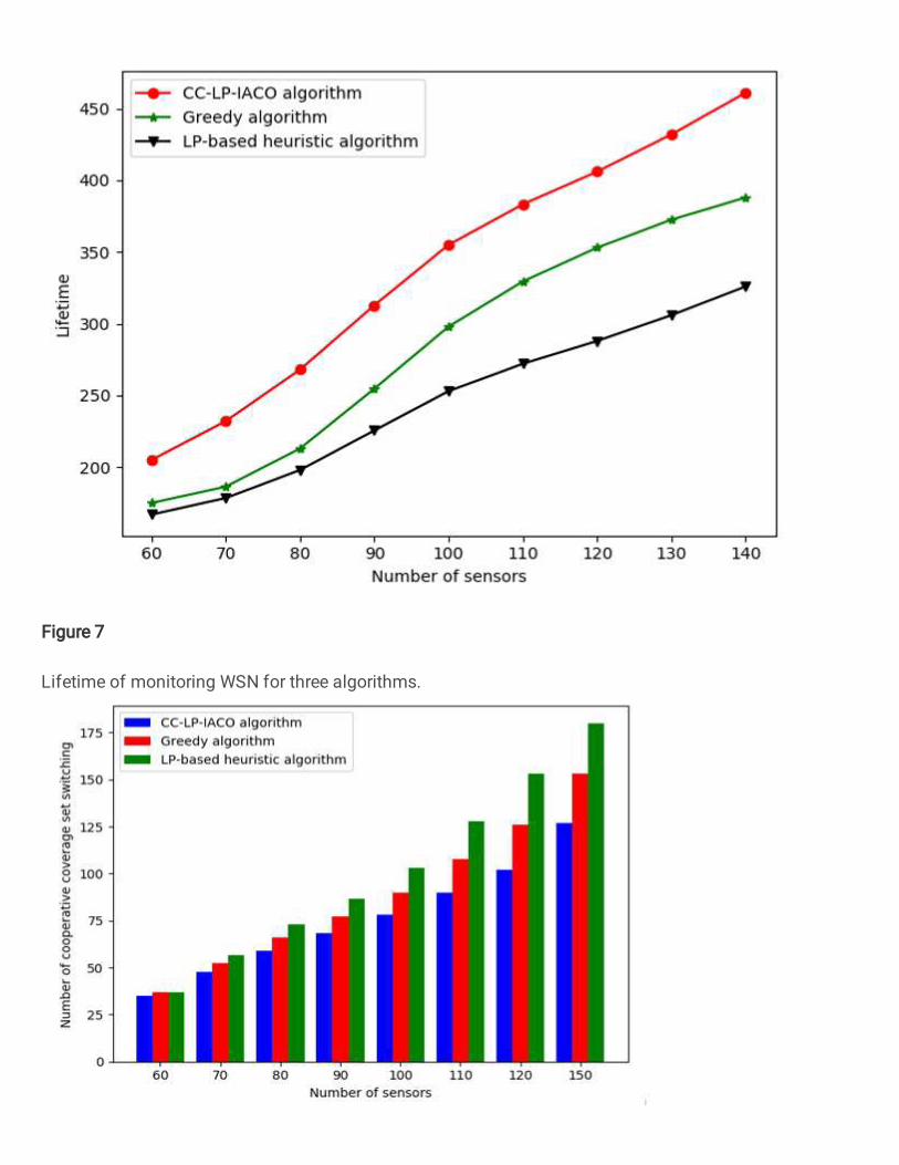
Figure 7
Lifetime of monitoring WSN for three algorithms.

Figure 8
Number of cooperative coverage set switching for three algorithm.