cooperative uavs formation reconfiguration in an … · uav tactics can be either centralized as a...

Paper: ASAT-16-131-US

16th

International Conference on

AEROSPACE SCIENCES & AVIATION TECHNOLOGY,

ASAT - 16 – May 26 - 28, 2015, E-Mail: [email protected]

Military Technical College, Kobry Elkobbah, Cairo, Egypt

Tel : +(202) 24025292 – 24036138, Fax: +(202) 22621908

Cooperative UAVs Formation Reconfiguration in an Obstacle-

Loaded Environment via Model Predictive Control

Ahmed Taimour Hafez∗, Sidney N. Givigi∗∗

Abstract: Recently, Unmanned Aerial Vehicles (UAVs) have attracted a great deal of

attention in academic, civilian and military communities as prospective solutions to a wide

variety of applications. The use of cooperative UAVs has received growing interest in the last

decade and this provides an opportunity for new operational paradigms. In this paper, the

problem of formation reconfiguration for a group of N cooperative UAVs in an obstacle-

loaded environment is solved using decentralized Learning Based Model Predictive Control

(LBMPC). The formation of the multiple cooperative UAVs respects the general rules of

flocking known as Reynold’s rules. Each UAV is required to avoid collision with nearby

flockmates, attempts to match the velocity of other team members and attempts to stay close

to other team members respecting the desired formation. When static obstacles appear, the

UAVs are required to steer around the obstacle or pass through avoiding collision with the

obstacles or with each other. A state transformation algorithm is applied to linearize the UAV

dynamics generating a linear system allowing the implementation in real life. Our main

contribution in this paper lays in solving the formation reconfiguration problem for a group of

cooperative UAVs forming a desired formation using decentralized LBMPC in the presence

of obstacles.

Keywords:Unmanned Aerial Vehicles, Cooperative UAVs, Learning Based

Model Predictive Control

1. Introduction

Due to their great importance especially in the last decade, UAV attracts a great attention and

concern in both the military and civilian communities and the efforts in their researches and

development have gained a great attention through the whole world. Objects like unmanned

aircraft, underwater exploiters, satellites and intelligent robotics are widely investigated as

they have potential applications.[1, 2].

∗ Egyptian Armed Forces, Egypt, e-mail: [email protected] ∗∗ Associate Professor in the ECE Department, Royal Military Collage (RMC), Canada, e-mail:[email protected]

mailto:[email protected]

mailto:[email protected]


In the last two decades, a great deal of effort has been invested in the development of

unmanned aerial vehicles (UAVs). UAVs are interesting alternatives to manned aircraft for

missions that can be dangerous for the human crew. They are also attractive for missions

where automation can improve the efficiency such as surveillance and inspection. These

autonomous vehicles are widely investigated as they have potential applications [1].

New UAVs’ capabilities and flexibility provide an opportunity for new operational

paradigms. These vehicles are developed to be capable of working in different circumstances

and weather conditions with some assistance of human control, also these vehicles have the

ability to handle complicated or uncertain situations. These vehicles may have different

shapes, sizes, configuration and characteristics. UAV is either described as a single air vehicle

(with associated surveillance sensors), or a UAV system, which usually consists of three to

six air vehicles, a ground control station, and support equipment [3].

With the increase in the cooperative UAVs applications performed in the civilian and military

communities, the need of a general strategies to control the performance of the autonomous

cooperative UAVs started to get the attention in research. These general strategies are defined

as the approaches used by the co-operative vehicles during the execution of their missions and

are denoted as UAV tactics [4].

UAV tactics can be either centralized as a single centralized decision maker in the team is

responsible to transmit the coordinated instructions to the other members; or decentralized, in

which each member is responsible for take its own control decision. UAV tactics can be

classified into [4]:

• Swarming and formation

• Task / Target assignment

• Formation reconfiguration

• Dynamic encirclement

Formation reconfiguration is defined as the dynamic ability of a UAV team to change their

formation according to the surrounding circumstances and due to the response to different

external factors such as changing of the mission, UAV team populations and surrounding

environments. A guidance law for formation reconfiguration of a group of cooperative UAVs

is needed to satisfy requirements of optimality and constraints of short computational time.

The new UAVs formation must guarantee safety, also, it must be compatible with the UAV

dynamics and may be governed by time constraint to pass between obstacles.

Formation reconfigurations have different behaviors according to the following factors

affecting the UAV team [5]:

• Changing the position of UAVs during mission execution.

• Combining small groups to form a large group according to the required

mission.

• Breaking a large group into smaller group to perform more than one

application at the same time.


Some of the main formation structure approaches are:

1. LeaderFollowerApproach:In this approach, some UAVs in the team are

designed as leaders while others are followers. Its main advantage is that it

can be easily understood and implemented but its main disadvantage is that it

is not robust in case of leader failure [6, 7, 8].

2. Virtual Structure Approach:In this approach, the whole team is treated

as a single rigid body and instead of following a certain path, each UAV

follows a certain moving point which allows them to be attached to each

other. In this case, the formation is treated as a single object which increases

robustness. On the other hand, it can only perform synchronized maneuvers

and it cannot deal with obstacle avoidance constraints or reject external

disturbances [9].

3. Behavior Based Approach:A desired behavior is designed for each UAV,

including the required information for mission, goal seeking and collision

avoidance. The control action of each UAV is a weighted average of the

control for each behavior and it is suitable for uncertain environments but it

lacks theoretical guarantees of stability [10].

There is a large amount of research in the field of formation reconfiguration for multiple cooperative UAVs. The range of applications is steadily growing including applications such as surveillance, exploration of regions, creating decoys, delivery of payloads (i.e. distributing ground based sensor networks), and radar and communication jamming [11, 12, 13, 14].

For instance, in [14], a robust control algorithm accompanied with a higher level path generation method is used to control the structure of a group of cooperative UAVs. The goal was to perform formation change maneuvers with a guaranteed safe distance between the different members of the team throughout the whole mission. The robust control ensures the stability of the formation during maneuver while the path generation method provides the vehicle with the safe paths. In [15], a dual mode control strategy was used to control the navigation of an UAV formation in a free and an obstacle-laden environment. In the obstacle-free environment, the safe mode was used and the danger mode was activated in the presence of obstacles to avoid collision using the Grossberg neural network (GNN).

The control of a group of autonomous cooperative UAVs performing various missions and applications is consider a great challenge in the field of robotic control and artificial intelligence. The designed controller has to modify the response and behavior of the non-linear systems to meet certain performance requirements and to respect the dynamics and hard constraints of UAV system. Therefore, MPC is a good control technique for this problems as MPC is characterized by its ability to handle difficult states and control inputs constraints, taking into account actuator limitations and allowing operation within constraints [16, 17].


In the field of cooperative UAVs formation, MPC has been used to solve the optimization control problem for a group of autonomous vehicles in different formation reconfiguration tactic [15, 18, 19].For instance, in [19], a non-linear MPC was used to control the formation of a fleet of UAVs in the presence of obstacles and collision avoidance. The UAV formation depends on a virtual reference point strategy, while the obstacle avoidance was guaranteed by adding a new cost penalty and inter-vehicle collision avoidance is guaranteed by a collision cost penalty, using the delayed neighboring information, combined with a new priority strategy.

Recently, control designers started to investigate the effect of adding a learning algorithm to the predictive decentralized approach especially MPC. Applying the learning algorithm to the MPC will improve the performance of the system andguarantee safety, robustness and convergence in the presence of states and control inputs constraints. In [20], the stabilization problem of a quadrotor in a desired altitude was solved using LBMPC. During the flight, a dual extended kalman filter (DEKF) was used as a method for learning by the quadrotor to learn about its uncertainties, while an MPC was used to solve the optimization control problem. In [21], LBMPC was used by a single quadrotor to learn to catch a ball during flight.

Our main contribution in this paper lays in solving the problem of formation reconfiguration for a group of cooperative UAVs using a decentralized LBMPC in an obstacle-loaded environment. A state transformation technique combined with a decentralized LBMPC and a collision avoidance technique are used to solve the formation reconfiguration problem. The state transformation technique introduces a linear model equivalent to the UAV non-linear dynamics, while the decentralized LBMPC compensates these non-linear dynamics using the learning technique and solves the optimization control problem using the MPC. Finally, the collision avoidance algorithm will steer the UAVs around the obstacles or pass between them avoiding collision with them.

The paper is organized as follows. We start with a discussion of theof notation used throughout the paper in Section II, followed by the problem formulation and the control objectives in Section III. The development of the decentralized LBMPC is introduced in Section IV, while in Section V, we present the results of our simulations. Section VI presents the conclusion of the work as well as discusses some future work.

2. Preliminaries

In this section, we define the notations used in this paper. Vectors are not typesetspecially, but will be identified as such when introduced (e.g. ,). All vectors are column vectors. We use superscript to denote the transpose of a matrix A and to denote the transpose of a vector .


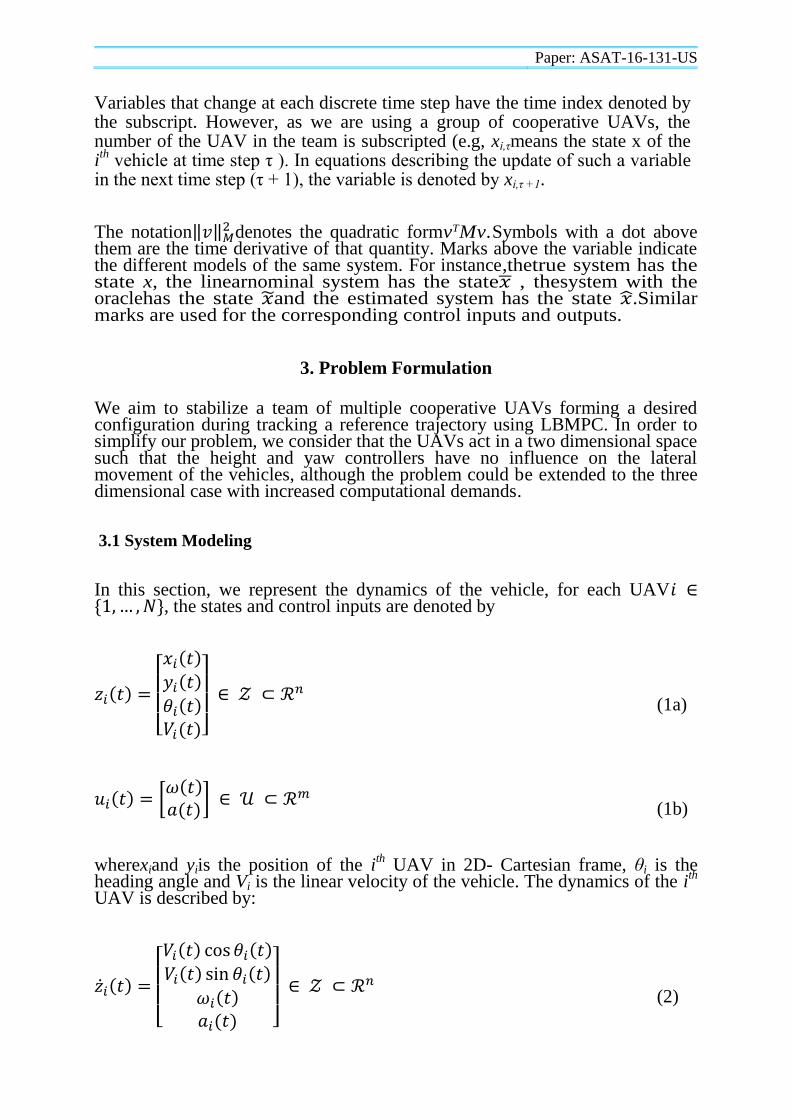
Variables that change at each discrete time step have the time index denoted by the subscript. However, as we are using a group of cooperative UAVs, the number of the UAV in the team is subscripted (e.g, xi,τmeans the state x of the ith

vehicle at time step τ ). In equations describing the update of such a variable in the next time step (τ + 1), the variable is denoted by xi,τ +1.

The notation denotes the quadratic formvTMv.Symbols with a dot above

them are the time derivative of that quantity. Marks above the variable indicate the different models of the same system. For instance,thetrue system has the state x, the linearnominal system has the state , thesystem with the oraclehas the state and the estimated system has the state .Similar marks are used for the corresponding control inputs and outputs.

3. Problem Formulation

We aim to stabilize a team of multiple cooperative UAVs forming a desired configuration during tracking a reference trajectory using LBMPC. In order to simplify our problem, we consider that the UAVs act in a two dimensional space such that the height and yaw controllers have no influence on the lateral movement of the vehicles, although the problem could be extended to the three dimensional case with increased computational demands.

3.1 System Modeling

In this section, we represent the dynamics of the vehicle, for each UAV , the states and control inputs are denoted by

(1a)

(1b)

wherexiand yiis the position of the ith UAV in 2D- Cartesian frame, θi is the

heading angle and Vi is the linear velocity of the vehicle. The dynamics of the ith

UAV is described by:

(2)


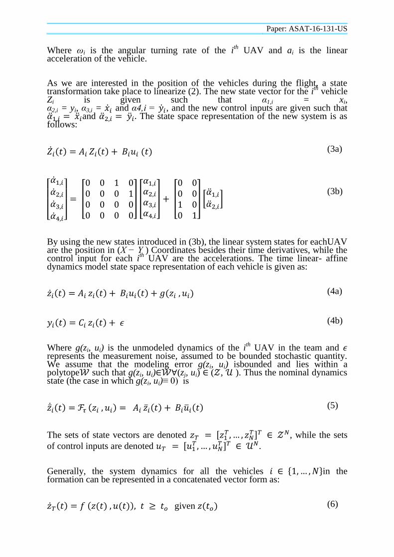
Where ωi is the angular turning rate of the ith UAV and ai is the linear

acceleration of the vehicle.

As we are interested in the position of the vehicles during the flight, a state transformation take place to linearize (2). The new state vector for the i

th vehicle

Zi is given such that α1,i = xi, α2,i = yi, α3,i = and α4,i = , and the new control inputs are given such that and The state space representation of the new system is as follows:

(3a)

(3b)

By using the new states introduced in (3b), the linear system states for eachUAV are the position in (X − Y ) Coordinates besides their time derivatives, while the control input for each i

th UAV are the accelerations. The time linear- affine

dynamics model state space representation of each vehicle is given as:

(4a)

(4b)

Where g(zi, ui) is the unmodeled dynamics of the ith UAV in the team and

represents the measurement noise, assumed to be bounded stochastic quantity. We assume that the modeling error g(zi, ui) isbounded and lies within a polytope such that g(zi, ui) ∀(zi, ui) ( , ). Thus the nominal dynamics state (the case in which g(zi, ui)≡ 0) is

(5)

The sets of state vectors are denoted

, while the sets

of control inputs are denoted

.

Generally, the system dynamics for all the vehicles in the formation can be represented in a concatenated vector form as:

given (6)


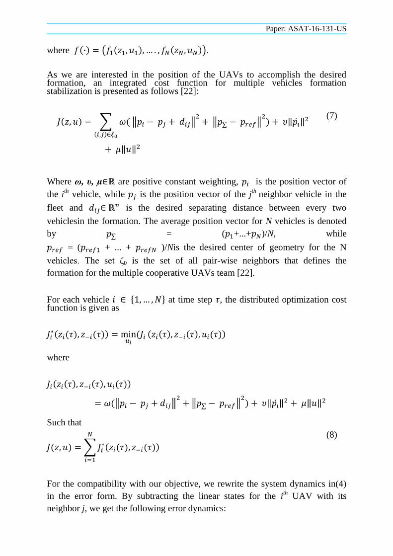
where .

As we are interested in the position of the UAVs to accomplish the desired formation, an integrated cost function for multiple vehicles formation stabilization is presented as follows [22]:

(7)

Where ω, υ, µ are positive constant weighting, is the position vector of

the ith

vehicle, while is the position vector of the jth

neighbor vehicle in the

fleet and is the desired separating distance between every two

vehiclesin the formation. The average position vector for N vehicles is denoted

by = ( +...+ )/N, while

= ( + ... + )/Nis the desired center of geometry for the N

vehicles. The set ζ0 is the set of all pair-wise neighbors that defines the

formation for the multiple cooperative UAVs team [22].

For each vehicle at time step , the distributed optimization cost function is given as

∗

where

Such that

∗

(8)

For the compatibility with our objective, we rewrite the system dynamics in(4)

in the error form. By subtracting the linear states for the ith UAV with its

neighbor j, we get the following error dynamics:


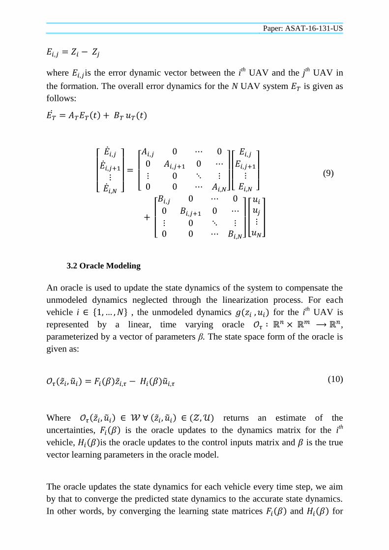
where is the error dynamic vector between the ith UAV and the j

th UAV in

the formation. The overall error dynamics for the N UAV system is given as

follows:

(9)

3.2 Oracle Modeling

An oracle is used to update the state dynamics of the system to compensate the

unmodeled dynamics neglected through the linearization process. For each

vehicle i , the unmodeled dynamics for the ith UAV is

represented by a linear, time varying oracle ,

parameterized by a vector of parameters β. The state space form of the oracle is

given as:

(10)

Where ∀ returns an estimate of the

uncertainties, is the oracle updates to the dynamics matrix for the ith

vehicle, is the oracle updates to the control inputs matrix and is the true

vector learning parameters in the oracle model.

The oracle updates the state dynamics for each vehicle every time step, we aim

by that to converge the predicted state dynamics to the accurate state dynamics.

In other words, by converging the learning state matrices and for


the ith

vehicle to zero, the predicted system dynamics will be similar to the

accurate UAV system dynamics.

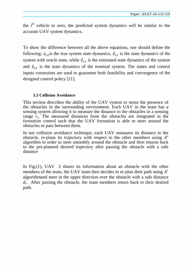
To show the difference between all the above equations, one should define the

following: is the true system state dynamics, is the state dynamics of the

system with oracle state, while is the estimated state dynamics of the system

and is the state dynamics of the nominal system. The states and control

inputs constraints are used to guarantee both feasibility and convergence of the

designed control policy [21].

3.3 Collision Avoidance

This section describes the ability of the UAV system to sense the presence of the obstacles in the surrounding environment. Each UAV in the team has a sensing system allowing it to measure the distance to the obstacles in a sensing range rs. The measured distances from the obstacles are integrated in the formation control such that the UAV formation is able to steer around the obstacles or pass between them.

In our collision avoidance technique, each UAV measures its distance to the obstacle, re-plans its trajectory with respect to the other members using ∗ algorithm in order to steer smoothly around the obstacle and then returns back to the pre-planned desired trajectory after passing the obstacle with a safe distance

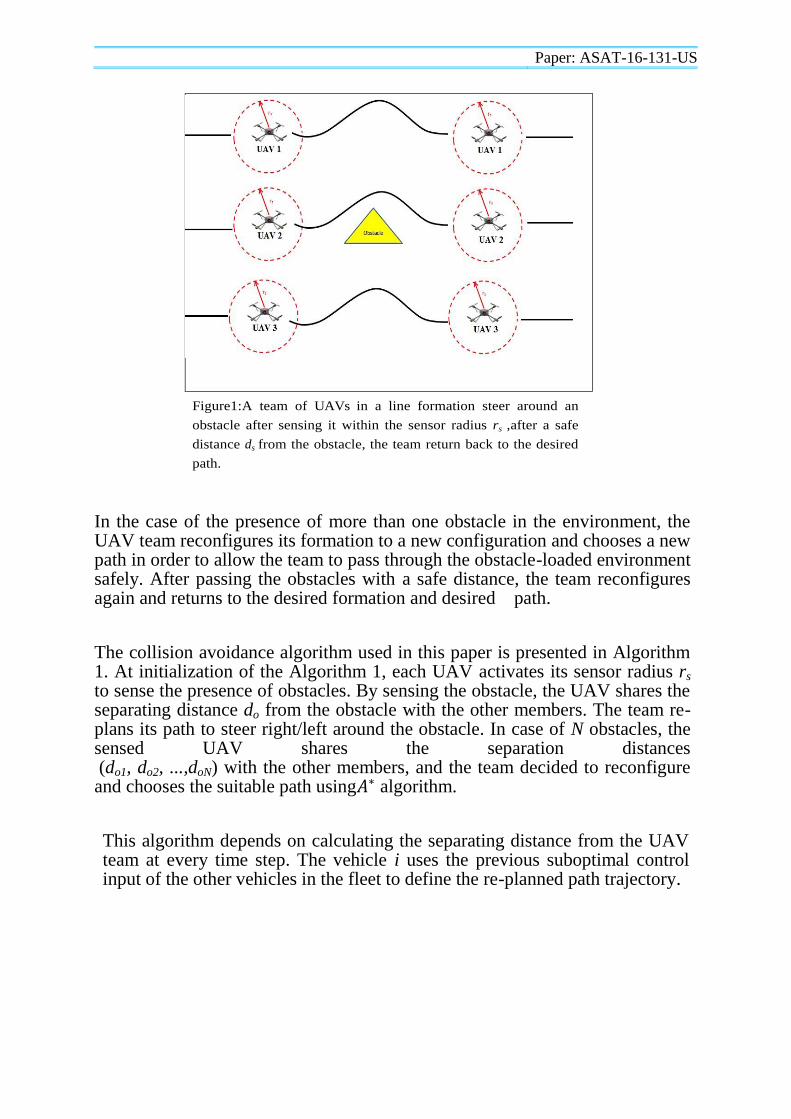
In Fig.(1), UAV 2 shares its information about an obstacle with the other

members of the team, the UAV team then decides to re-plan their path using ∗ algorithmand steer in the upper direction over the obstacle with a safe distance

ds. After passing the obstacle, the team members return back to their desired

path.


Figure1:A team of UAVs in a line formation steer around an

obstacle after sensing it within the sensor radius rs ,after a safe

distance ds from the obstacle, the team return back to the desired

path.

In the case of the presence of more than one obstacle in the environment, the UAV team reconfigures its formation to a new configuration and chooses a new path in order to allow the team to pass through the obstacle-loaded environment safely. After passing the obstacles with a safe distance, the team reconfigures again and returns to the desired formation and desired path.

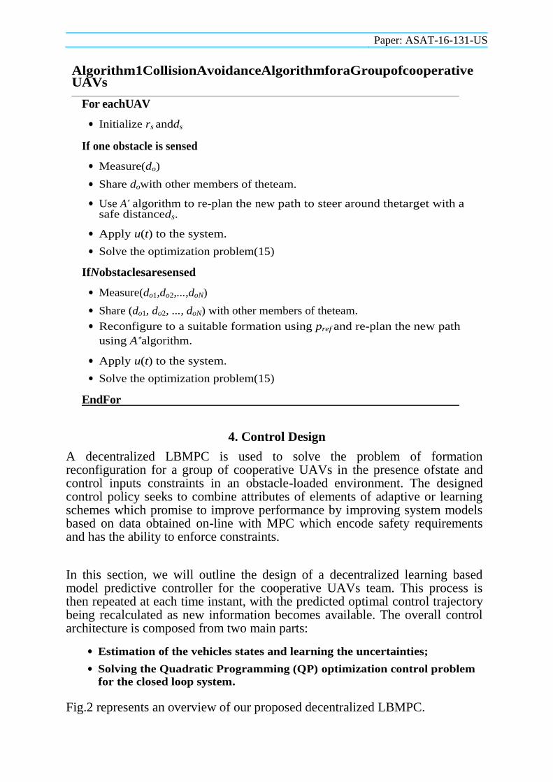
The collision avoidance algorithm used in this paper is presented in Algorithm 1. At initialization of the Algorithm 1, each UAV activates its sensor radius rs to sense the presence of obstacles. By sensing the obstacle, the UAV shares the separating distance do from the obstacle with the other members. The team re-plans its path to steer right/left around the obstacle. In case of N obstacles, the sensed UAV shares the separation distances (do1, do2, ...,doN) with the other members, and the team decided to reconfigure and chooses the suitable path using ∗ algorithm.

This algorithm depends on calculating the separating distance from the UAV team at every time step. The vehicle i uses the previous suboptimal control input of the other vehicles in the fleet to define the re-planned path trajectory.


Algorithm1CollisionAvoidanceAlgorithmforaGroupofcooperativeUAVs

For eachUAV

• Initialize rs andds

If one obstacle is sensed

• Measure(do)

• Share dowith other members of theteam.

• Use A∗ algorithm to re-plan the new path to steer around thetarget with a safe distanceds.

• Apply u(t) to the system.

• Solve the optimization problem(15)

IfNobstaclesaresensed

• Measure(do1,do2,...,doN)

• Share (do1, do2, ..., doN) with other members of theteam.

• Reconfigure to a suitable formation using pref and re-plan the new path

using A∗algorithm.

• Apply u(t) to the system.

• Solve the optimization problem(15)

EndFor

4. Control Design

A decentralized LBMPC is used to solve the problem of formation reconfiguration for a group of cooperative UAVs in the presence ofstate and control inputs constraints in an obstacle-loaded environment. The designed control policy seeks to combine attributes of elements of adaptive or learning schemes which promise to improve performance by improving system models based on data obtained on-line with MPC which encode safety requirements and has the ability to enforce constraints.

In this section, we will outline the design of a decentralized learning based model predictive controller for the cooperative UAVs team. This process is then repeated at each time instant, with the predicted optimal control trajectory being recalculated as new information becomes available. The overall control architecture is composed from two main parts:

• Estimation of the vehicles states and learning the uncertainties;

• Solving the Quadratic Programming (QP) optimization control problem

for the closed loop system.

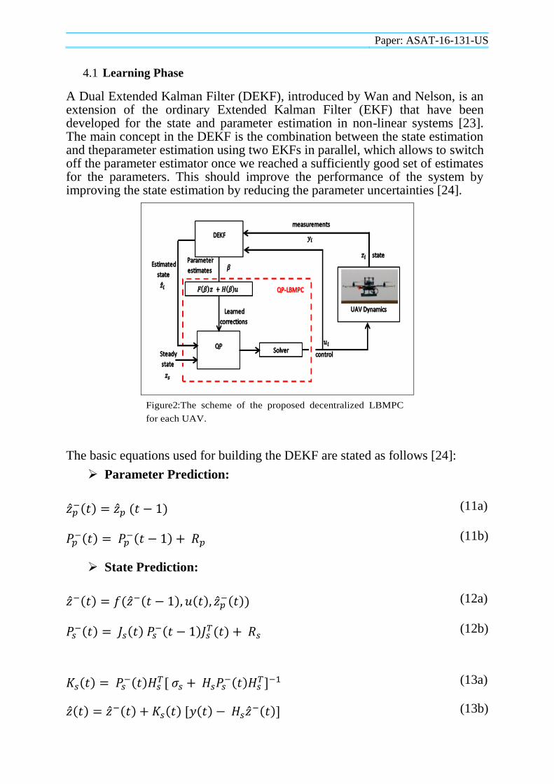
Fig.2 represents an overview of our proposed decentralized LBMPC.


4.1 Learning Phase

A Dual Extended Kalman Filter (DEKF), introduced by Wan and Nelson, is an extension of the ordinary Extended Kalman Filter (EKF) that have been developed for the state and parameter estimation in non-linear systems [23]. The main concept in the DEKF is the combination between the state estimation and theparameter estimation using two EKFs in parallel, which allows to switch off the parameter estimator once we reached a sufficiently good set of estimates for the parameters. This should improve the performance of the system by improving the state estimation by reducing the parameter uncertainties [24].

Figure2:The scheme of the proposed decentralized LBMPC

for each UAV.

The basic equations used for building the DEKF are stated as follows [24]:

Parameter Prediction:

(11a)

(11b)

State Prediction:

(12a)

(12b)

(13a)

(13b)


State Correction:

Parameter Correction:

Where is the estimated state vector, the estimated parameter vector, u is

the control input vector and y is the measurement vector. The error covariance

matrix of the state vector is denoted by , while the error covariance matrix of

the parameter vector is denoted by . Also, and are the user specified

process noise covariance matrcies for the state and parameter estimators,

respectively, while the corresponding output noise covariance matrcies for the

state and parameter estimators are denoted by and , respectively.

Moreover, and are the DEKF gain matrcies for the state and the

parameter, respectively, while and are the Jacobian matrcies of the

output for state/parameter estimator and is the Jacobian matrices for state

estimates.

4.2 Optimization Phase

A decentralized MPC controller, based on the idea of tube-MPC, is combined

with the learning algorithm introduced in section 4.1 to control the cooperative

UAVs during performing their desired formation. For the decentralized

LBMPC prediction horizon M , by given a nominal trajectory, the true

trajectory for each agent i is guaranteed to lie within the MPC tube around the

given trajectory.

At the heart of the LBMPC control scheme is the on-line solution of a convex

optimization problem. The optimization cost function will contain the learning

part for each vehicle in the team

(13c)

(14a)

(14b)

(14c)


(15)

subject to:

(16)

where M is the predication horizon, is the predicted dynamic states of the

ith

vehicle while denote the vector of the estimated dynamic state of the

neighbors of iand is the optimal control inputs to the system. The

polyhedral sets and are bounded and convex; they encode the allowable

states control inputs, respectively.

Marrices P, Q and R are semi-definite positive matrices weights on the final state srror cost, the intermediate state error cost and the control input cost, respectively. Moreover, the desired state is denoted by , while is the steady state control that would maintain the desired steady state , the nominal feedback gain Ki serves to limit the effect of model uncertainty for agent i and it is chosen so that the discrete-time algebraic Ricatti equation (DARE)

(17)

is satisfed. Finally, the actual control inputs in (16) are used to determine the predicted learning dynamic states in (15) and the predicted nominal state used for constraint satisfaction in (16) for the i

th vehicle.

5. Simulation Results

The control strategy discussed in sections 3 and 4 is successfully implemented in simulation by a team of cooperative UAVs consists of three vehicles. The objective of this simulation is to show that, the designed control policy is fit for solving the problem of formation reconfiguration for a group of cooperative UAVs in an obstacle-loaded environment. One should notice that the solutions found in this paper may be scaled to accommodate larger teams of UAVs in more complex environments.


As discussed in 3.3, each UAV has a sensor radius rs = 15m to sense the presence of obstacles. By sensing the obstacle, the UAV shares the obstacle information with the other members. The UAV team decided to change its path and steer/pass through around the obstacles smoothly with a safe distance ds = 10m. After passing the obstacle, each UAV re-calculates the desired path and return back to the desired formation. Moreover, in case of different obstacles, the UAVs cooperate to choose the optimum formation and steer/pass through the obstacles safely.

One can summarize the requirements of our simulations to be as follows:

• Separation distance dref = 10m between each two neighborvehicles.

• Matched velocity between all members of theteam.

• The ability of the team to re-plan its path to avoidobstacles.

The simulation can be run for different formation structures and with different number of vehicles which prove the robustness of our designed control policy. For all simulations, the prediction horizon is M = 5, simulation time is T = 24s and the sampling time is τ = 0.2s.

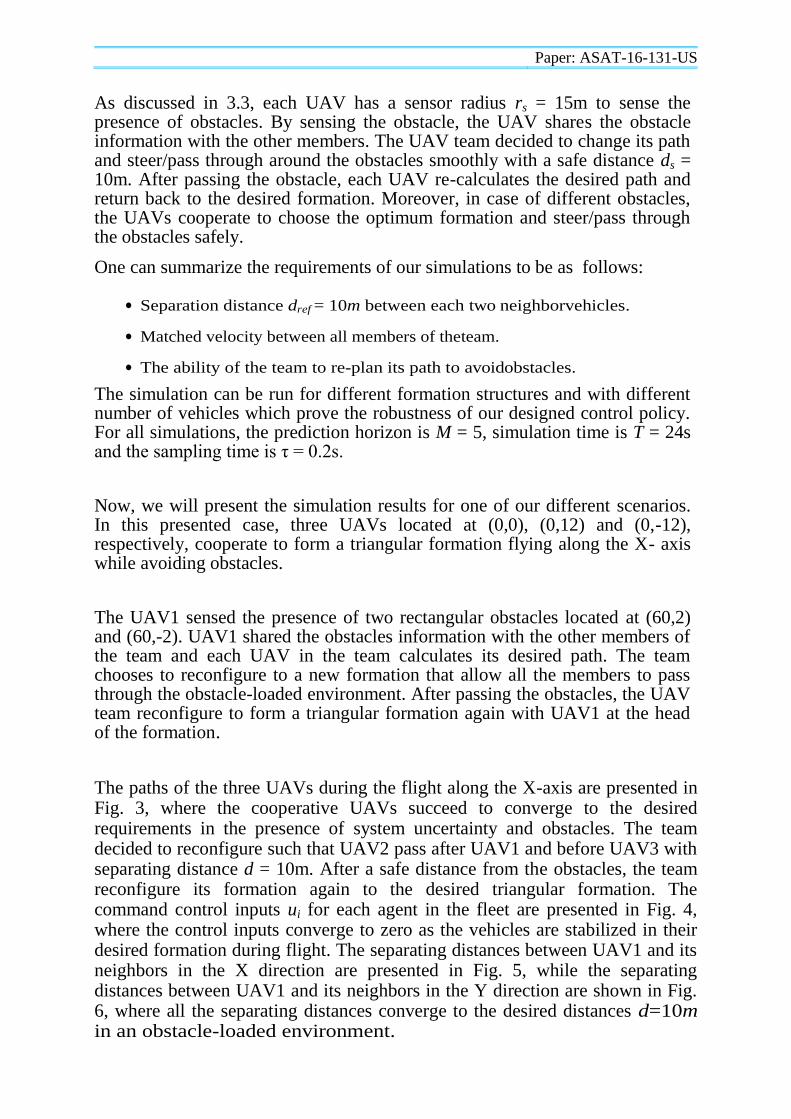
Now, we will present the simulation results for one of our different scenarios. In this presented case, three UAVs located at (0,0), (0,12) and (0,-12), respectively, cooperate to form a triangular formation flying along the X- axis while avoiding obstacles.

The UAV1 sensed the presence of two rectangular obstacles located at (60,2) and (60,-2). UAV1 shared the obstacles information with the other members of the team and each UAV in the team calculates its desired path. The team chooses to reconfigure to a new formation that allow all the members to pass through the obstacle-loaded environment. After passing the obstacles, the UAV team reconfigure to form a triangular formation again with UAV1 at the head of the formation.

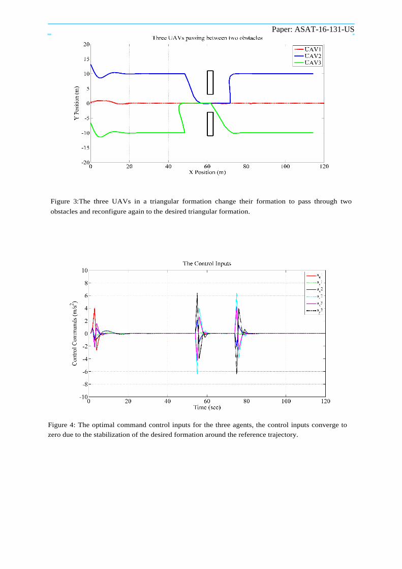
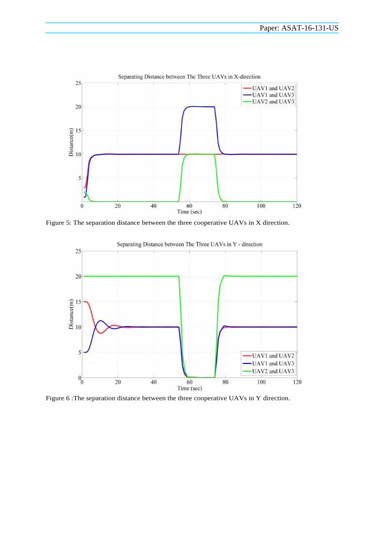
The paths of the three UAVs during the flight along the X-axis are presented in Fig. 3, where the cooperative UAVs succeed to converge to the desired requirements in the presence of system uncertainty and obstacles. The team decided to reconfigure such that UAV2 pass after UAV1 and before UAV3 with separating distance d = 10m. After a safe distance from the obstacles, the team reconfigure its formation again to the desired triangular formation. The command control inputs ui for each agent in the fleet are presented in Fig. 4, where the control inputs converge to zero as the vehicles are stabilized in their desired formation during flight. The separating distances between UAV1 and its neighbors in the X direction are presented in Fig. 5, while the separating distances between UAV1 and its neighbors in the Y direction are shown in Fig. 6, where all the separating distances converge to the desired distances d=10m in an obstacle-loaded environment.


Figure 3:The three UAVs in a triangular formation change their formation to pass through two

obstacles and reconfigure again to the desired triangular formation.

Figure 4: The optimal command control inputs for the three agents, the control inputs converge to

zero due to the stabilization of the desired formation around the reference trajectory.


Figure 5: The separation distance between the three cooperative UAVs in X direction.

Figure 6 :The separation distance between the three cooperative UAVs in Y direction.


References

[1]G.Cai,K.Lum,B.Chen,andT.Lee,“Abriefoverviewonminiaturefixed-wing unmanned

aerial vehicles,” in 8th IEEE International Conference on Control and Automation

(ICCA),2010. IEEE,2010,pp.285–290.

[2] A. Alshbatat and Q. Alsafasfeh, “Cooperative decision making using a collection of autonomous quadrotor unmanned aerial vehicle interconnected by a wireless communicationnetwork.”

[3]E. Boneand C. Bolkcom, “Unmanned aerial vehicles: Background and issues for congress.” DTIC Document,2003.

[4]A.Marasco,S.N.Givigi,andC.A.Rabbath,“Dynamicencirclementofamoving target using decentralized nonlinear model predictive control,”Amer-icanControlConference,pp.3966–3972,2013.

[5]A.Ryan,M.Zennaro,A.Howell,R.Sengupta,andJ.Hedrick,“Anoverviewof emerging

results in cooperative UAV control,” in 43rd IEEE Conferenceon Decisionand

Control (CDC),vol.1. IEEE,2004,pp.602–607.

[6] K. Do and J. Pan, “Nonlinear formation control of unicycle-

typemobilerobots,”RoboticsandAutonomousSystems,vol.55,no.3,pp.191–204,2007.

[7]D.Scharf,F.Hadaegh,andS.Ploen,“Asurveyofspacecraftformationflyingguidanceand

control.partii:control,”inAmericanControlConference,2004.Proceedingsofthe2004,v

ol.4. IEEE,2004,pp.2976–2985.

[8]Y.Ding,C.Wei,andS.Bao,“DecentralizedformationcontrolformultipleUAVs based on leader-following consensus with time-varying delays,” in2013ChineseAutomationCongress(CAC).IEEE,2013,pp.426–431.

[9]W.RenandR.Beard,“A decentralized scheme for spacecraft formation flying via the

virtual structure approach,” in American Control

Conference,2003.Proceedingsofthe2003,vol.2. IEEE,2003,pp.1746–1751.

[10]J.Lawton,R.Beard,andB.Young,“A decentralized approach to formation maneuvers,

”IEEETransactionsonRoboticsandAutomation,vol.19,no.6,pp. 933–941,2003.

[11]R.Olfati-Saber,“Flockingformulti-agent dynamic systems: Algorithms and theory,

”IEEETransactionsonAutomaticControl,vol.51,no.3,pp.401–420,2006.

[12]H.Rezaee,F.Abdollahi,andM.B.Menhaj,“Model-freefuzzyleader-follower formation

control of fixed wing UAVs,

”in201313thIranianConferenceonFuzzySystems(IFSC).IEEE,2013,pp.1–5.

[13]D.Luo,T.Zhou,andS.Wu,“Obstacleavoidanceandformationregroupingstrategy and

control for UAV formation flight,” in 10th IEEE International Conference on

Control and Automation (ICCA), 2013. IEEE, 2013,pp.1921–1926.

[14]G.RegulaandB.Lantos,“FormationcontrolofalargegroupofUAVswithsafepathplannin

g,”in21stMediterraneanConferenceonControl&Automa-tion (MED). IEEE, 2013,

pp.987–993.

[15]X.Wang,V.Yadav,andS.Balakrishnan,“CooperativeUAVformationflyingwith

obstacle/collision avoidance,” IEEE Transactions on ControlSystemsTechnology,.


[16] E. F. Camacho and C. Bordons, Model Predictive Control. London:Springer-

Verlag,2007.

[17]R.Negenborn,B.DeSchutter,M.Wiering,andH.Hellendoorn,“Learningbased model

predictive control for markovdecision processes,”

inProceedingsofthe16thIFACworldcongress,2005,pp.1–7.

[18]J.Lavaei,A.Momeni,andA.G.Aghdam,“Amodelpredictivedecentralizedcontrol scheme with reduced communication requirement for spacecraft formation, ”IEEETransactionsonControlSystemsTechnology, vol.16,no.2,pp. 268–278,2008.

[19]Z.Chao,S.-L.Zhou,L.Ming,andW.-

G.Zhang,“UAVformationflightbasedonnonlinearmodelpredictivecontrol,”Mathema

ticalProblemsinEngineer-ing, vol. 2012,2012.

[20]A.Aswani,P.Bouffard,andC.Tomlin,“Extensions of learning-based model predictive control for real-time application to a quadrotor helicopter,”inAmericanControlConference(ACC),2012.IEEE,2012,pp.4661–4666.

[21]P.Bouffard,A.Aswani,andC.Tomlin,“Learning-basedmodelpredictivecontrol on a

quadrotor: Onboard implementation and experimental results,

”IEEEInternationalConferenceonRoboticsandAutomation(ICRA), 2012.IEEE, 2012,

pp.279–284.

[22] W. B. Dunbar and R. M. Murray, “Distributed receding horizon controlformultivehicleformationstabilization,”Automatica,vol.42,no.4,pp.549–558,2006.

[23] E. A. Wan and A. T. Nelson, “Dual extended kalman filter ethods,”Kalmanfiltering

and neural networks, pp. 123–173,2001.

[24]T.A.Wenzel,K.Burnham,M.Blundell,andR.Williams,“Dualextendedkalmanfilterforve

hiclestateandparameterestimation,”VehicleSystemDynamics,vol.44,no.2,pp.153–171,2006

cooperative uavs formation reconfiguration in an … · uav tactics can be either centralized as a...

Documents