coordinating development: can income-based incentive schemes eliminate pareto inferior equilibria?

Journal of Development Economics 83 (2007) 368–391www.elsevier.com/locate/econbase

Coordinating development: Can income-based incentiveschemes eliminate Pareto inferior equilibria?☆

Philip Bond a, Rohini Pande b,⁎

a University of Pennsylvania, United Statesb Yale University, United States

Received 11 May 2004; received in revised form 8 August 2006; accepted 26 August 2006

Abstract

Individuals' inability to coordinate investment may significantly constrain economic development. Inthis paper we study a simple investment game characterized by multiple equilibria and ask whether anincome-based incentive scheme can uniquely implement the high-investment outcome. A general propertyof this game is the presence of a crossover-investment point at which an individual's incomes frominvestment and non-investment are equal. We show that arbitrarily small errors in the government'sknowledge of this crossover point can prevent unique implementation of the high-investment outcome. Weconclude that informational requirements are likely to severely limit a government's ability to use income-based incentive schemes as a coordination device.© 2006 Elsevier B.V. All rights reserved.

JEL classification: O12; D62; H23Keywords: O20

1. Introduction

Whenever investment decisions are decentralized but individual returns to investmentremain dependent on the choices made by others, economic activity may be limited by acoordination failure among the agents. This observation has often been taken to be particularly

☆ The authors are from the University of Pennsylvania and Yale University respectively. We are grateful to Debraj Ray,two anonymous referees and, especially, Dilip Mookherjee for detailed comments. We also thank Dino Gerardi, StephenMorris and Andrew Newman for helpful comments. Bond thanks the Institute for Advanced Study for hospitality andfinancial support (in conjunction with Deutsche Bank) over the academic year 2002–03. Any errors remain ours.⁎ Corresponding author.E-mail address: [email protected] (R. Pande).

0304-3878/$ - see front matter © 2006 Elsevier B.V. All rights reserved.doi:10.1016/j.jdeveco.2006.08.004

mailto:[email protected]

http://dx.doi.org/10.1016/j.jdeveco.2006.08.004

369P. Bond, R. Pande / Journal of Development Economics 83 (2007) 368–391

relevant for low-income countries. A large theoretical literature, starting with Rosenstein-Rodan(1943) and Hirschman (1957), has explored how coordination failures can cause poor countriesand people to stay poor (see, e.g., Murphy et al., 1989; Matsuyama, 1996; Becker et al., 1990).

If one takes seriously the view that economic growth is inhibited by coordination failures,then a natural question is whether suitably designed public policies can prevent such failures.Import substitution industrialization policies, for instance, are widely viewed as just such anattempt, although there is widespread skepticism about their success (Krueger, 1997; Bhagwati,1993). In general, however, discussions of whether or not a government can coordinateeconomic development have remained largely informal and have rarely progressed beyond theobservation that a government's inability to directly observe individual investment decisionsmay prevent such coordination (Rodrik, 1996, and again Krueger, 1997). Put differently, thegovernment's inability to observe individual actions makes coordination a multi-agent moralhazard problem.

However, as is now well known, the appropriate design of contracts can mitigate agencyconcerns in moral hazard problems. In the standard example, an employee is paid according toobservable output. A suitably designed wage scheme will induce the agent to take the employer'spreferred, though unobservable, action. In a public policy context (e.g. Mirrlees' 1971 seminalwork on income taxation) the analogue is a tax and transfer policy which depends on observedoutcomes (an individual's market income), but not on unobserved actions. In keeping with thisline of research, this paper examines whether a tax and transfer policy can be used as acoordination device when the government does not observe individual actions.

In the canonical coordination game an agent's income depends both on her action and theactions of all other agents in the economy. As a result the game has multiple Pareto-rankedequilibria.1 In this spirit, we consider an economy in which a continuum of agents must eachdecide whether or not to invest.2 The returns to both investment and non-investment depend onthe proportion of investors, which we denote as η. The social optimum is for all agents toinvest. Individual incomes from non-investment exceed those from investment when η=0, withthe opposite true when η=1. Hence, although it is an equilibrium for all agents to invest, it isalso an equilibrium for no agent to invest. Moreover, there is an intermediate level ofinvestment, η say, at which investment and non-investment generate the same returns. We castthe problem of coordination of economic activity as a principal–agent problem in which asingle principal – the government – seeks to provide multiple agents with the incentive toinvest.

If the government can directly observe individual investments then coordinating the full-investment equilibrium is straightforward. Indeed, Rodrik (1996) has argued that informationgathering by institutions such as the Japanese MITI was key to the success of the industrialpolicies pursued by East Asian governments. However, previous discussions of governmentcoordination have also noted that, in practice, a government bureaucrat may find it difficult todistinguish between genuine investment and consumption disguised as investment. That is, agovernment's lack of information constrains its ability to foster coordination and henceeconomic development.

1 Cooper (1999) reviews the coordination game literature, while Hoff (2000) and Ray (2000) discuss its relevance formodeling market outcomes in low-income countries.2 Our description of the investment game is similar to those in “big push” models of development— industrialization is

individually profitable only if a sufficiently large number of agents industrialize (see, for instance, Murphy et al., 1989).

370 P. Bond, R. Pande / Journal of Development Economics 83 (2007) 368–391

Our main results both reinforce and develop the view that information is critical tosuccessful coordination — and that in practice, the informational hurdle is hard to clear. Westart from the point where previous informal discussions end: is there anything a governmentcan do if it cannot observe individual investment decisions? We allow a government to maketransfers to individuals based on their incomes, and likewise to engage in income taxation.3

Given this, we ask whether there exist tax/transfer schemes such that all agents investing is theonly stable equilibrium.

Recall that when η individuals invest, investment and non-investment yield the sameincome. Investors and non-investors appear identical to the government at the investmentlevel η; as such, there is necessarily an equilibrium at that point. Our main results relate tothe difficulties this engenders for successful coordination. Specifically, it is reasonable toregard a government coordination policy as successful only if it leaves η=1 as the onlystable equilibrium. In other words, η must be an unstable equilibrium when the policy is inplace. To ensure this the government's policy must leave investors with higher post-tax/transfer income both when just more and just less than η of the population invest.

Consider first the class of government policies in which each individual's transfer dependsonly on that individual's pre-transfer income. Coordination is only feasible if the governmentknows the exact value of η, along with the corresponding income at that point. We show(Proposition 2) that if instead it makes even an arbitrarily small mistake in identifying thesevalues, then coordination fails. The reason is that the policy creates a stable equilibrium inthe vicinity of η. To the extent small misperceptions are inevitable, we interpret this result asindicating that coordination using this class of policies is impossible.

Second, we consider a broader class of government policies in which each individual'stransfer can also depend on the full distribution of incomes in the “economy”. In this casecoordination is often feasible. Specifically, if the externality associated with investment issufficiently strong then a government can successfully use information on the proportion ofinvestors at different income levels to ensure that post-transfer returns from investment alwaysexceed those from non-investment. However, we believe that such policies are much harder fora government to successfully implement. In particular, the relevant “economy” is the set ofindividuals actually affected by the externalities in question. If the government fails tocorrectly identify this, then it likewise misidentifies the income distribution, and itscoordination policy will fail. This problem is made even more relevant by the fact thatinvestment games are typically played out at the sectoral level, and an economy consists ofmultiple sectors. Again, the informational requirements that a coordination policy must meetappear substantial.

1.1. Related literature

Our analytic approach is related to the literature on implementation in moral-hazardsettings — see Ma (1988), Arya et al. (1995), Arya et al. (1997), and Chung (1999).4 Thefirst three of these papers address a problem noted by Mookherjee (1984): when a principalseeks to provide incentives to many agents, the optimal incentive scheme may possessmultiple equilibria. Ma shows that, in general, the use of “integer” message games can

3 Since we do not impose budget balancing, these two options allow for the same outcomes.4 The standard implementation problem concerns an adverse-selection setting (see Maskin, 1999). That is, agents first

learn their type, which a planner then seeks to induce them to report truthfully.


eliminate the multiplicity of equilibria. The papers of Arya, Glover and their co-authors ruleout the use of such mechanisms on grounds of realism, and show that in specific instances ofthe many-agent incentive problem unwanted equilibria can still be eliminated. Closest to us isChung (1999) who examines whether a specific class of policies, affirmative action policies,can implement the unique efficient (human capital) investment equilibrium.

1.2. Paper outline

The remainder of the paper is structured as follows. Section 2 describes the economicenvironment. Section 3 identifies necessary features of a tax scheme which implements thehigh-investment outcome. Section 4 considers implementation via policies based onindividual income, and Section 5 policies which also condition on the income distribution.Section 6 discusses the robustness of our results under alternative assumptions and Section 7concludes.

2. Environment

2.1. Basics

The economy consists of a continuum of risk-neutral agents. Every agent faces a discreteinvestment choice, a∈{0, 1}, where a=1 is interpreted as investment. Investment choice ayields a monetary return of y≡ fa(η), where η is the fraction of agents who invest.

We assume fa (·) is a continuous, twice-differentiable function. An agent's decision toinvest generates positive spill-overs for other investors, i.e., f1′ (·)N0. In contrast, f0′ (·)≷0.However, f0′ (·)=0 at only finitely many values of η, and so investment affects the returnsto non-investment almost everywhere. The externalities investment generates for investorsexceed those generated for non-investors, i.e., | f1′ (·)|N | f0′ (·)|. Fη denotes the incomedistribution when a fraction η invest. The income distribution collapses to a one-pointdistribution whenever incomes from investment and non-investment coincide. Otherwise, itis a two-point distribution — a proportion 1−η of the population has income f0(η) and aproportion η income f1(η).

A principal, who we refer to as the government, seeks to design a mechanism to affectagents' investment decisions. We restrict the government to transfer schemes T ( y) thatdetermine the post-transfer income of an agent with pre-tax income y. We consider, in turn, thecases where T only depends on an agent's income, y, and where it can also depend on the fullincome distribution F. In both cases we assume that T is a continuous function of y and F, inthe following sense. Let F denote the set of distribution functions on the real line that placemass on at most two points. For any pair of sequences fyngoR and fFngoF such that yn→yand Fn (ϵ)→F (x) for all x except the mass points of F, T ( yn, Fn)→T ( y, F ).5 For the mostpart we restrict attention to mechanisms that do not make use of messages; in Section 6 wediscuss more general mechanisms of this type.

We impose no other restrictions on T. In particular, we do not require budget balancing —there is no reason the investment externality should encompass the whole economy.

5 That is, convergence in distribution (see, e.g.,Billingsley, 1995). We discuss the restriction to continuous tax/transferfunctions T in Section 6.


Finally, when we refer to the economy absent government intervention, we simply meanT ( y, F )≡y, i.e., no net taxes or transfers.

2.2. Equilibrium

Given a fraction η of investors, let ΔT (η) denote the gain to an agent from investing instead ofnot investing :

DT ðgÞuTð f1ðgÞ;FgÞ − Tð f0ðgÞ;FgÞ

We assume that, absent government intervention, full-investment (η=1) maximizes socialwelfare, i.e.,

1a arg maxg

g f1ðgÞ þ ð1− gÞ f0ðgÞ

We next define our concept of equilibrium and stability for this economic environment, anduse these definitions to characterize a coordination game.

Definition 1. Nash equilibriumGiven a government policy T, a fraction η of agents investing is a Nash equilibrium if and only

if η=0 and ΔT (0)≤0, or η=1 and ΔT (1)≥0 or η∈ (0,1) and ΔT (η)=0.

Throughout we refer to an equilibrium by the fraction that invest in that equilibrium, η.

Definition 2. StabilityAn equilibrium η is unstable if there exists δ such that either ΔT (η−ε)b0 for all ε∈ (0, δ ), or

ΔT (η+ε)N0 for all ε∈ (0, δ ). An equilibrium that is not unstable is stable.

The notion of equilibrium stability consists of asking whether individuals' optimal-investment strategies are immune to small perturbations of the proportion of investors aroundthe presumed equilibrium, i.e., to investor noise. Below (see Proposition 2) we show thatarbitrarily small government misperceptions of the economic fundamentals create new stableequilibria. The sizes of the basins of attraction of the newly created stable equilibria (i.e., theextent of investor noise) depend on the extent of government misperceptions. It follows that ourdefinition of stability is premised on the assumption that investor noise is less than governmentnoise. If we interpret the notion of equilibrium stability as reflecting the outcome of a learningprocess among investors (in the face of strategic uncertainty) then an economic interpretation ofthis assumption is that, relative to the government, investors are faster at “learning” about theireconomic environment.

Since we have assumed that f1′N0 and | f1′| N | f0′| , the function ΔT is strictly increasing absentgovernment intervention (i.e., T ( y)≡y). Consequently, absent intervention there are threepossible equilibrium sets in our economy: η=0 is the only stable equilibrium; η=1 is onlystable equilibrium; and η=0 and η=1 are both stable equilibria, with an unstable equilibrium ata unique investment level point η∈ (0, 1). For the remainder of the paper we assume that thelast of these three cases holds, and refer to our economy as a coordination game. Fig. 1illustrates a coordination game. (In Section 7, we briefly discuss the problem of ensuring full-

Fig. 1. A linear example of a coordination game.


investment when the only stable equilibrium absent intervention is η=0. This case is, of course,a manifestation of the “free-rider” problem.6 )

Since investment and non-investment incomes coincide at the investment level η∈ (0, 1),necessarily ΔT (η)=0 for all government policies T. That is, investment by a fraction η of agentsis an equilibrium. Given this, the most that can be hoped of a government policy is that it leaveη=1 as a stable equilibrium, but η as an unstable equilibrium:

Definition 3. ImplementationA policy T implements η if η is the only stable equilibrium.Implementation when individual actions are publicly observable is straightforward: tax the

socially inefficient action, or subsidize the socially efficient action.7 More formally, consider thepolicy T (a=1, y, F ) = y and T (a=0, y, F ) = f1 (0) − ε, some εN f1 (0)− y. This policy only taxesnon-investors, such that they prefer investing. Under this choice of T, full-investment is the onlyequilibrium. The remainder of the paper considers implementation when agents' incomes, but notactions, are observable.

3. Implementation

In selecting the parameters of the tax and transfer scheme the government's aim is to eliminatethe no-investment equilibrium (η=0), while preserving full-investment as a stable equilibrium(η=1). We start by noting:

Proposition 1. Δ must be positive

Suppose that either (1) ΔT ≡0 over some interval [η−ε, η ]⊂ [ 0, 1], or (2) ΔT (η )b0 forsome η∈ [ 0, 1]. Then there is a stable equilibrium to the left of η.

Proof of Proposition 1. The returns to investment and non-investment f0 and f1 are continuousin η. Continuity of T implies that ΔT is continuous. If condition (1) holds, clearly any point

6 A simple example of the free-rider problem in our economy is f0 (η)=5/8+η/2 and f1(η)=η. Investment has positiveexternalities for both investors and non-investors, the socially efficient investment level is η=1, yet the only equilibriumis at η=0.7 This was the case considered by Pigou (1932).


η′∈ (η−ε, η) is a stable equilibrium. If condition (2) holds then either there exists η′bη such thatΔT (η′)N0, and so there must be a stable equilibrium between η′ and η; or else ΔT (η′)≤0 for allη′bη, in which case η=0 is a stable equilibrium. □

Proposition 1 immediately implies two restrictions on implementation via income-basedincentive schemes.

The first restriction relates to the fact that an individual's pre-transfer income from non-investment exceeds that from investment when the fraction of investors is less than η. FromProposition 1, we know that any tax and transfer scheme that implements full-investment mustleave investors with a higher after-transfer income than non-investors. Consequently, the tax andtransfer scheme must be non-monotonic in pre-transfer income: over some range, income must betaxed at more than 100%. An immediate corollary is that implementation is infeasible if economicagents can costlessly burn money.

More formally, assume an agent with true income y can costlessly reduce her income to anyθ∈ [0, y ]. This transforms a tax/transfer scheme as follows. Given T, an agent chooses incomeha arg maxha½0;y�TðhÞ. (Since T is continuous and [0, y] is compact, T (θ) has a well-definedmaximum over [0, y].) So the effective transfer scheme is

T eff ð yÞ ¼ maxha½0;y�

T h� �

:

Trivially T eff is weakly increasing in y. It is easily shown to be continuous. Consequently:

Corollary 1. If agents can costlessly burn money, implementation of full-investment isimpossible.

The second restriction relates to the existence of an investment level η at which investor andnon-investor incomes coincide. Proposition 1 tells us that implementation requires that the post-transfer returns from investment must everywhere (weakly) exceed those from non-investment.However, if investment entails even a small non-pecuniary cost ϵ then under any tax/transferpolicy investors are worse off than non-investors when the investment level is η. As such, a stableequilibrium will exist to the left of η:

Corollary 2. If investment entails a strictly positive non-pecuniary cost then implementation offull-investment is impossible.

Corollaries 1 and 2 identify two serious impediments to the possibility of implementing full-investment. In the next section, we show that even if a non-monotonic tax/transfer scheme isviable (i.e., burning money is not possible), and there are no non-pecuniary costs of investment,implementation of full-investment remains extremely challenging. Consistent with informaldiscussions of coordination policies, our analysis highlights the key role played by governmentinformation (or its lack thereof ).

4. Policies based on individual income

We start with the case where the transfer policy, T, can only be conditioned on an agent'sincome. We know from Proposition 1 that implementing full-investment requires that aftertaxes and transfers investment yields a higher income level for all η. Non-investment yields a

Fig. 2. The tax/transfer scheme T= y +γ| y− y |.


higher income when less than η invest but not when more than η invest. Hence, T must ensurethat higher incomes are penalized when fewer than η invest, but rewarded when more than ηinvest.

It follows that the tax/transfer policy T must be at a minimum at the income level at whichinvestment and non-investment incomes coincide, i.e., at y ¼ f0ðgÞ ¼ f1ðgÞ. When T isdifferentiable, a somewhat loose argument is as follows. Since DT ðgÞ ¼ 0, it follows fromProposition 1 that ΔT must be at a local minimum at η — else, there exists a point η such thatΔT (η)b0, which is inconsistent with implementation of full-investment. Taking derivatives ofΔT gives

DTVðgÞ ¼ f1VðgÞT Vð f1ðgÞÞ � f0VðgÞT Vð f0ðgÞÞDWT ðgÞ ¼ f1VðgÞ2 � f0VðgÞ2

� �TWðyÞ

Then ΔT′ (η)=0 implies T′ ( y)=0, while ΔT″ (η)≥0 and | f1′ |N | f0′ | imply T ″ ( y)≥0. Moreformally:

Lemma 1. Intersection pointsAny scheme T that implements full-investment (η=1) must have a local minimum at y= f1 (η).

Proof of Lemma 1. See AppendixThe following example illustrates Lemma 1. Assume income from investment is f1 (η)=η+x1,

while that from non-investment is f0(η)=x0−βη. Also, assume β∈ (0, 1), x0Nx1 and 1+x1≥x0−β,so that absent government intervention no-investment and full-investment are both stable equilibria.

When a fraction g ¼ x0−x11þ b

invest both investment and non-investment incomes equal

y ¼ x1 þ x0−x11þ b

. Lemma 1 suggests it is natural to consider a tax/transfer policy with a minimum

at y. One class of policies with this property, illustrated in Fig. 2, is

T ¼ yþ gj y − y j

Fig. 3. Implementing full-investment: the solid lines represent investment incomes, the dashed lines non-investmentincomes, and the heavy lines after-tax/transfer incomes. For all η after-tax/transfer incomes are higher for investors thannon-investors.


where γ N0 is a constant. This specification of T is continuous in y and implements η=1 asfollows. First, if η b η invest then the pre-transfer incomes of investors are lower than thoseof non-investors; but their post-transfer incomes are higher since the externalitiesexperienced by investors are stronger, and so | f1 (η) − y | N | f0(η) − y |. Second, if η N ηinvest then both the pre-transfer and post-transfer incomes of investors exceed those of non-investors. So ΔT (η)N0 for all η other than η, and η=1 is the only stable equilibrium. Fig.3 provides a graphical illustration.

However, implementation is extremely sensitive to small imperfections in governmentinformation. To see this, consider the specific policy with γ=1(so that T ( y)=2y−y for y≤ y,and T ( y)=y otherwise) and assume the government wrongly estimates the returns to investingas f1 (η)+ ( x1−x1), where x1≠x1. We depict this possibility in Fig. 4.

Suppose the government overestimates investment returns, i.e., x1Nx1. In this case,incomes in the neighborhood of y are unaffected, and consequently ΔT (η)=0, with ΔT

(η)b0 immediately to the left of η. There is now a stable equilibrium to the left of η.Suppose instead the government underestimates investment returns, i.e., x1bx1. Then incomesaround y are reversed, making η a stable equilibrium — whereas absent the tax/transfer policyit was unstable.

In this example arbitrarily small errors in the government's knowledge of the economycause implementation to fail. We show that this sensitivity of implementation to thegovernment's information is a general property of the environment.

In more general terms than before, a government may misperceive the returns toinvestment as g, in place of the true returns, f1.

8 Let G be the metric space consisting of allcontinuous, increasing and twice-differentiable functions from [0, 1] to the positive real line,with metric jj g− hjj ¼ R jg− hj 8g; haG. It is reasonable to regard the government'smisperception as small whenever || f1−g || is small, i.e., when

gafhaGj jjh− f1jjb eguBeð f1Þ

8 Proposition 2 (see below) also holds if we restrict attention to the specific case analyzed in the example, i.e., mistakesof the form f1 (η)+k, for some constant k.

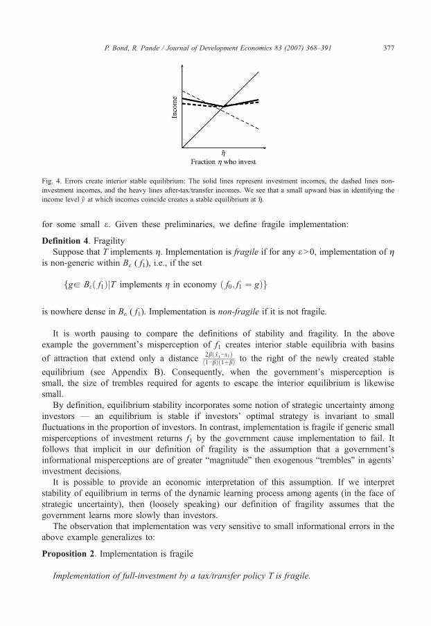
Fig. 4. Errors create interior stable equilibrium: The solid lines represent investment incomes, the dashed lines non-investment incomes, and the heavy lines after-tax/transfer incomes. We see that a small upward bias in identifying theincome level y at which incomes coincide creates a stable equilibrium at η.


for some small ε. Given these preliminaries, we define fragile implementation:

Definition 4. FragilitySuppose that T implements η. Implementation is fragile if for any εN0, implementation of η

is non-generic within Bε ( f1), i.e., if the set

fga Beð f1ÞjT implements g in economy ð f0; f1 ¼ gÞg

is nowhere dense in Bε ( f1). Implementation is non-fragile if it is not fragile.

It is worth pausing to compare the definitions of stability and fragility. In the aboveexample the government's misperception of f1 creates interior stable equilibria with basins

of attraction that extend only a distance 2bð x1−x1Þð1−bÞð1þbÞ to the right of the newly created stable

equilibrium (see Appendix B). Consequently, when the government's misperception issmall, the size of trembles required for agents to escape the interior equilibrium is likewisesmall.

By definition, equilibrium stability incorporates some notion of strategic uncertainty amonginvestors — an equilibrium is stable if investors' optimal strategy is invariant to smallfluctuations in the proportion of investors. In contrast, implementation is fragile if generic smallmisperceptions of investment returns f1 by the government cause implementation to fail. Itfollows that implicit in our definition of fragility is the assumption that a government'sinformational misperceptions are of greater “magnitude” then exogenous “trembles” in agents'investment decisions.

It is possible to provide an economic interpretation of this assumption. If we interpretstability of equilibrium in terms of the dynamic learning process among agents (in the face ofstrategic uncertainty), then (loosely speaking) our definition of fragility assumes that thegovernment learns more slowly than investors.

The observation that implementation was very sensitive to small informational errors in theabove example generalizes to:

Proposition 2. Implementation is fragile

Implementation of full-investment by a tax/transfer policy T is fragile.

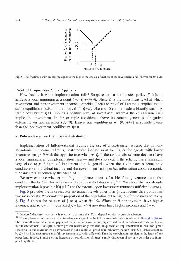
Fig. 5. The fraction ξ with an income equal to the higher income as a function of the investment level (shown for ηb1/2).


Proof of Proposition 2. See Appendix.How bad is it when implementation fails? Suppose that a tax/transfer policy T fails to

achieve a local minimum at a point y= f1 (η)= f0(η), where η is the investment level at whichinvestment and non-investment incomes coincide. Then the proof of Lemma 1 implies that astable equilibrium exists in the interval [0, η+ε], where εN0 can be made arbitrarily small. Astable equilibrium ηN0 implies a positive level of investment, whereas the equilibrium η=0implies no investment. In the example considered above investment generates a negativeexternality on non-investors ( f0′b0). Hence, any equilibrium η∈ (0, η+ε] is socially worsethan the no-investment equilibrium η=0.

5. Policies based on the income distribution

Implementation of full-investment requires the use of a tax/transfer scheme that is non-monotonic in income. That is, post-transfer income must be higher for agents with lowerincome when ηb η with the opposite true when ηb η. If the tax/transfer scheme does not havea local minimum at y, implementation fails — and does so even if the scheme has a minimumvery close to y. Failure of implementation is generic when the tax/transfer scheme onlyconditions on individual income and the government lacks perfect information about economicfundamentals, specifically the value of η.

We now examine whether non-fragile implementation is feasible if the government can alsocondition the tax/transfer scheme on the income distribution Fη.

9,10 We show that non-fragileimplementation is possible if η≠1/2 and the externality on investment returns is sufficiently strong.

Fig. 5 provides the intuition. For investment levels other than η, the income distribution hastwo mass points. We denote the proportion of the population at the higher of these mass points byξ. Fig. 5 shows the relation of ξ to η when ηb1/2. When ηb η non-investors have higherincomes, and so ξ=1−η; conversely, when ηN η investors have higher incomes and ξ=η.

9 Section 7 discusses whether it is realistic to assume that T can depend on the income distribution.10 The implementation problem when transfers can depend on the full income distribution is related to Battaglini (2006).The main difference between our paper and his is that we show unique implementation of the full-investment equilibriumin our environment. Battaglini's more general results only establish uniqueness of implementation in coalition–proofequilibria. In our environment no-investment is not a coalition–proof equilibrium whenever f0 (η)b f1 (1) (this is impliedby f0′b0 and the assumption that full-investment is socially efficient). Thus the coordination problem at the heart of ourpaper (and, indeed, in much of the literature on coordination failures) simply disappears if we only consider coalition–proof equilibria.


For non-fragile implementation, the important point is that income distributions withξ≤1/2 only arise when the investment level is between η and g ¼ 1

2N g. Moreover, for alarge enough investment externality, the income of investors when ηN1/2 exceeds theincome level of both non-investors and investors for any ηb η.

Non-fragile implementation can then be achieved as follows. If ξ≤1/2, it must be thatηN η, and so individuals with higher incomes should receive higher post-transfer incomes.Moreover, if ξN1/2 but the higher income exceeds maxη∈[0, η ] f0(η), then again it must bethat ηN η, and so individuals with higher incomes should receive higher post-transferincomes. Finally, if ξN1/2 but the higher income level is less than maxη∈[0,η] f0(η) then itmust be that ηb η, and so individuals with higher incomes should receive lower post-transfer incomes.

A similar scheme is possible when η N1/2 (see the Proof of Proposition 3). Moreover, itis worth stressing that the requirement that the externality is sufficiently strong is sufficientbut not necessary. That is, all that is required is that when ξ N1/2, the government canrobustly distinguish the distribution when η=1−ξ invest from that when η=ξ invest. Whenexternalities are strong this is easily established, but it will be true much more generally.However, for the purposes of presenting a reasonably concise constructive proof, we focuson the case of strong externalities. Formally, our result is:

Proposition 3. Non-fragile implementation

Provided η≠1/2, and the externality on investment is sufficiently large (i.e., f1′ large enough),there exists a tax/transfer policy T such that for all f 1 sufficiently close to f1 full-investment is theonly stable equilibrium.

Proof of Proposition 3. The text above gives the main idea. The main difficulty encountered inthe formal proof is defining T such that it is continuous on the space F of distributions. The proofis relegated to the Appendix.

6. Some extensions

We conclude our analysis with a discussion of the robustness of our results to four features ofour model.

6.1. Continuity of tax scheme

Our analysis assumes that the tax/transfer policy T is continuous — both in an agent'sincome y and in the income distribution F when this is also an argument. Does thisassumption matter? The main issue with allowing T to depend on incomes y in adiscontinuous fashion is that it allows the government to eliminate equilibria in veryunconvincing ways. For instance, consider the following simple example. The return toinvestment is f1 (η)=η while that to non-investment is f0ðgÞ ¼ 1þ2g

4 . Consider the tax/transfer policy

Tð yÞ ¼ − y if y V 3=8y if y N 3=8

�


Since f0(η)≤3/8 whenever η≤1/4 while f1 (η)≤3/8 whenever η≤3/8, this implies

DT ðgÞ ¼

−gþ 1þ 2g4

if ga 0;14

� �

−g−1þ 2g

4if ga

14;38

� �

g−1þ 2g

4if ga

3

8; 1

� �

8>>>>>>><>>>>>>>:

That is, ΔT (η) is strictly positive for η≤1/4, jumps to being negative and decreasing over(1/4, 3/8], and then is increasing over (3/8, 1]. The only stable equilibrium is η=1.

However, there is a strong sense in which η=1/4 should be considered a stable equilibrium. Ifjust less than η=1/4 invest, then more agents will invest; while if just more than η=1/4 invest,then fewer agents invest. Requiring that the tax/transfer policy T be continuous in y avoids suchproblems.

With regard to tax/transfer policies based on the income distribution, it suffices to note that, afortiori, Proposition 3 would still hold if T were allowed to be discontinuous.

6.2. Message games

Thus far we have restricted attention to tax/transfer policies that rely solely on pre-taxincomes observed by the government. We now examine whether the government can dobetter by using a scheme where it also collects messages from agents. We consider a gamewhere agents make investment decisions and submit messages to the government. Thegovernment then observes incomes and implements transfers. We restrict attention to finitemessage spaces; we denote the message space by M.11 We continue to distinguish betweenschemes which only make use of individual incomes, and those that use the fulldistribution.

A scheme that uses only individual incomes and individual messages is equivalent to oneusing only individual incomes. To see this, consider a scheme T ( y, m) in which an agent'safter-transfer income is determined by his own pre-transfer income y and message m∈M.Define the scheme T ( y)≡maxm T ( y, m): that is, for any income y the government knowswhich message(s) provide an agent with the highest payoff, and so can design an alternatescheme that directly embeds this information. Clearly T has the same equilibria as T.

Of course, in general one would not expect a scheme conditioning on individualmessages to accomplish much. The main uses of message games in the literature involve acomparison of messages from different agents. As such, suppose next that a scheme cancondition both on the distribution of incomes and the distribution of messages.

First, recall that in our model conditioning on the income distribution is sufficient forcoordination under many circumstances — see Proposition 3. Under such circumstancesthere is clearly no scope for a transfer policy conditioning on the distribution of messagesto improve implementation relative to a transfer policy conditioning on the incomedistribution.

11 This avoids the possibility of “tail-chasing” schemes.


Second, even under circumstances in which Proposition 3 does not hold, there is no gain tousing a mechanism dependent on messages. By essentially the same argument as above, theequilibria under such a mechanism are the same as those under a suitably defined scheme inwhich messages are not used. The basic intuition is that since the agents do not observe anythingmore than the government does, messages cannot improve the outcome.12

Previous papers such as Ma (1988) have identified conditions under which message gamesexpand the set of implementable outcomes. The key reason why this does not occur in ourenvironment is that incomes are deterministic. Instead, in Ma's setting incomes are stochastic,and so the principal does not observe the stochastic income distribution conditional on eachagent's action. As such, the principal is able to acquire additional information about the agent'saction by asking him to submit a report. In contrast, in our setting the principal directlyobserves the (degenerate) stochastic distribution of an agent's income. It follows that messagesdo not improve the planner's ability to coordinate economic activity.

6.3. Nash implementation

We have focused throughout on Nash implementation: full-investment is implemented if it isthe only (stable) Nash equilibrium under the tax/transfer policy in effect. However, alternatenotions of implementation are possible. For example, one might instead ask whether full-investment is undominated Nash implementable: that is, is there a policy T under which full-investment is the only equilibrium when agents play undominated strategies?13

In our setting, undominated Nash implementation is straightforward. Recall that, byassumption, f1 (1)Nmaxη f0(η). Choose ŷ∈ (maxη f0(η), f1 (1)), and consider the policy

Tð yÞ ¼0 if y b y

f1ð1Þy − y

f1ð1Þ− y if yz y:

(

Under this policy, investment is strictly preferred when everyone else invests. Moreover, at anyinvestment level η, an agent's income from not investing is f0(η)bŷ, and so T ( y)=0. This is atleast weakly less than the agent's income from investing. Thus not investing is a weaklydominated strategy, while investing is an undominated strategy. Consequently, if we require thatagents use undominated strategies a tax/transfer scheme which conditions on own incomeimplements full-investment. Moreover, this scheme is robust to small informational mistakes.14

More generally, and in terms of ΔT, a policy implements full-investment in undominated Nashif ΔT (η)≥0 for all η, with ΔT (η)N0 for some η. The proof of Proposition 2 is easily adapted todeal with this alternate implementation concept, and implies that for non-fragile implementationin undominated Nash the policy T must be flat over some neighborhood around y.

12 A proof of this claim is available on the authors' webpages. Broadly speaking, the government can define a message-freescheme T that matches T when equilibrium messages are reported. Hammond (1979) and Guesnerie (1995) also establishconditions under which any outcome that is implementable by a general mechanism is also implementable using a simple taxmechanism. Both authors consider onlyweak implementation, while our result pertains to unique implementation (though is lessgeneral in other respects).13 A weakly dominated strategy is one such that an alternative strategy is weakly preferred no matter what other agentsdo, and is strictly preferred for at least some choice of strategies by other agents. An undominated strategy is one that isnot weakly dominated.14 We thank the editor for bringing this example to our attention.


The above example makes clear that this is straightforward to accomplish in our existingmodel. However, if we impose small frictions on the ability of the planner to do what itwants then complete flatness of the tax/transfer scheme is surprisingly hard to satisfy.

In particular, consider the case where there are two possible states L and H with (possiblysmall but differing) probabilities that the government will be forced to implement an arbitrarystatus quo policy. Such a set-up would, for instance, capture the case where an electedgovernment loses its majority status in the legislature and is, therefore, unable to implement itspreferred policy. We model the timing of this process as:

(1) The government announces its policy T.(2) Agents observe whether the state of the world is ω∈{L, H }.(3) Agents decide whether or not to invest.(4) With probability εω a “regime change” occurs: the government abandons its tax policy T, and

instead adopts T0. For concreteness, we take T0 to be the no-intervention policy, T0 ( y)≡y.(5) The government observes incomes and executes its policy.

First, note that this modeling perturbation does not eliminate the possibility of fragileimplementation. In particular, in the example we saw that T ( y)= y+γ | y − y | Nash implementsfull-investment. Under the possibility of regime change,

Tx ¼ ð1−exÞð1þ cÞ y þ ðex−ð1−exÞcÞy if y V y

ð1−exÞð1− cÞ yþðð1−exÞcþ exÞy if y N y

�

Provided (1−εω)γNεω for ω=L, H (i.e., the probability of regime change is small), full-investment is the only stable Nash equilibrium for ω=L, H.

However, non-fragile implementation in undominated Nash equilibrium is not possible in bothstatesω=L,H. From the agents' perspective, the tax policywhen theymake their investment decisionsis Tω=(1−εω )T+εωT0. The key point is that Tω cannot be flat around y for both states ω=L, H.

Finally, given that we have introduced small frictions on the ability of the government toimplement her preferred policy we may also want to weaken our implementation concept to allowfor virtual implementation in undominated Nash equilibrium (Abreu and Sen, 1991; Abreu andMatsushima, 1992). In our environment this is equivalent to asking whether full-investment canbe implemented with probability arbitrarily close to one? The answer is no: from the abovediscussion, the highest probability with which the full-investment equilibrium can beimplemented in the perturbed model is max{Pr (ω=H), Pr (ω=L)}b1.

6.4. Equilibrium stability

A related issue is our definition of stability. For concreteness, consider the following example:f1 (η)=η, f0(η)=3/4−η/2, and a tax policy defined by

Tð yÞ ¼

12þ g

38−y

� �if yb

38

12

if ya38;58

� �12þ g y−

58

� �if yN

58

:

8>>>>>><>>>>>>:


It is readily verified that ΔT (η) is positive up to 3/8, zero from 3/8 to 5/8, and positive from5/8 to 1.

Given our current definition of stability, this tax scheme fails to implement full-investment:investment levels in the range 3/8 to 5/8 are stable equilibria. However, these equilibria areclearly not as stable as an equilibrium η for which ΔT (η)=0 and ΔT is strictly decreasing at η.In particular, if stability relates to small mistakes by agents in playing the game, over timeagents will eventually “escape” to the right from any equilibrium in the interval 3/8 to 5/8. Inessence, these equilibria may be seen as “short-run” stable, but “long-run” unstable.

If we alter our definition of stability so as to classify equilibria of this type as unstable, thenfull-investment could be (at least) sometimes implemented in a non-fragile way. One suchinstance is the above example. However, as with alternate implementation concepts, Nashimplementation here depends critically on the government being able to impose a tax schemethat is completely flat over the income range around y. Again, although easily accomplished inour existing model, this is not possible in the perturbed model sketched above.

7. Discussion

This paper examines the use of income-based incentive schemes as a coordination device. Ina large economy generic implementation is infeasible if the scheme only conditions onindividual income. In contrast, coordination in a large economy is sometimes feasible if theplanner can use tax schemes which condition on both individual income and the incomedistribution. In a small economy, where generically an agent's income would reveal if she hasinvested or not, we would also expect coordination to be feasible.15

The main problem with implementation in a large economy arises from the existence of acrossover point η at which incomes from investment and non-investment coincide, not from theexistence of externalities per se. This is clearly seen when we consider implementation in afree-rider game, that is a game with externalities but a unique (inefficient) equilibrium.16 Ina free-rider game individual returns from investment vary with the number of investors but arealways below those from not-investing. Implementation is straightforward: choose a tax/transferthat rewards those with lower pre-tax incomes. Observe that f1′N f0′ implies that f1 (η)− f0 (η) isstrictly increasing. Since full-investment is not an equilibrium f1 (η)b f0(η) for all ηb1. Apolicy of the form T ( y)=Y−λy, where Y and λN0 are constants rewards those with lower pre-transfer incomes. Thus T ( f1 (η))NT ( f0(η)) for all ηb1. That is, full-investment (η=1) is theonly stable equilibrium. Moreover, implementation is insensitive to small errors in thegovernment's knowledge of the returns to investment, f1.

Overall, we are inclined to interpret our results as both reinforcing and developing thewidely held view that limited information constrains a government's ability to conduct asuccessful development policy based on coordination of investment activity. Coordinationusing policies that only condition on individual income fails whenever the government haseven arbitrarily small misperceptions regarding the fundamentals of the economy. In contrast,

15 Piketty (1993), for instance, shows that with a finite number of agents a tax schedule which conditions on the incomedistribution can achieve a first best allocation.16 The economics literature on how to achieve efficiency in the presence of externalities has, almost exclusively, focusedon free-rider games. Two much studied examples are the “tragedy of the commons” games where common access toresources leads agents to choose consumption levels in excess of the social optimum (see, e.g., Gordon, 1954), and “teamproduction games ” where, given a joint production process, team members under-provide effort (Holmström, 1982; alsosee Legros and Matthews, 1993; and Battaglini, 2006).


the high-investment equilibrium can be implemented with less exact knowledge if the tax/transfer policy is allowed to depend on the full distribution of incomes. However, thesuccessful execution of such a policy, in turn, presents its own informational challenges. Inparticular, it requires that the policy-maker know which individuals are actually affected by themultiple-equilibria generating externality. In practice, this is likely to be a non-trivial matter. Tosee this, consider an economy populated by many different groups. Individuals in each group(separately) decide whether to invest in a group-specific technology. The positive externalitygenerated by investment may only apply across individuals adopting the same technology. Ifthe principal does not know the group identity of agents, and if there are many groups, thenthe income distribution for each group is unobservable (Lanjouw and Lanjouw, 2001 discussthe widespread coexistence of multiple heterogeneous sectors in developing countries).

A quite different concern about mechanisms which depend on the whole income distributionis that they may require more commitment by the government than those which do not. Forinstance, suppose only the government observes all agents' incomes, while each agent onlyobserves his/her income. Then ex post the government will be tempted to implement thetransfer policy minFaFT ( y, F ): that is, give each agent the smallest transfer consistent withhis/her individual income. Only tax/transfer policies that are independent of the incomedistribution are immune from this type of problem.17

We would like to, however, end with a methodological counter to our policy pessimism. Arich literature has developed and used the techniques of implementation theory to analyze theefficient provision of public goods. However, few researchers have applied these techniques tothe field of development economics.18 This paper, we hope, both demonstrates the importanceof these techniques for development economics and, more specifically, suggests their usefulnessfor identifying policy mechanisms which are both feasible and robust to informationalconstraints.19

Appendix A. Proofs

The Proof of Lemma 1 requires the following result:

Lemma 2. Let T: RYR be a continuous function, with y; y a R such that T( y)bT( y). Thenthere exists y ≠ y such that | y− y |≤ | ŷ− y| and T ( y)NT ( y ) for all y such that | y− y|b | y − y|. Thatis, we can find a point y such that at all points closer to y the function T is strictly greater than at y (and y itself is closer to y than is ŷ ).

17 The auctions literature analyzes the possibility that mechanisms in which an agent's allocation depends on otheragents' messages maybe prone to cheating by the principal. Vickrey (1961) notes that a “second-price method may not beautomatically self-policing to quite the same extent as the top-price method”. Porter and Shoham (2004) show that asecond-price auction collapses to a first-price auction when the seller can costlessly “invent” bids.18 Exceptions include Rai (2002), who studies the design of credit programs, and Besley and Coate (1992), who analyzetargeting of public work programs.19 We conjecture that another promising research avenue would be to exploit insights offered by the global gamesliterature. This literature suggests that introducing uncertainty about economic fundamentals (in our set-up this wouldcorrespond to uncertainty about the shape of the investment functions, f0 and f1) can provide a natural form ofequilibrium selection. It would be interesting to ask whether a government can, by deliberately creating uncertainty aboutinvestment returns, cause there to be a unique equilibrium.


Proof of Lemma 2. For any εN0 and yaR let Bε ( y) denote the open interval ( y−ε,y+ε),while Bε ( y) denotes the closed interval [ y−ε, y+ε]. The proof is by contradiction. Supposethat contrary to the claimed result for any y∈ B | y−y |( y ) \ { y} there exists a y∈B| y−y |( y) suchthat T( y)≤T(y).

Since the function T is continuous it must obtain its infimum value over the closed intervalB | y−y | ( y). That is, the set A≡arg miny∈B| y− y |( y) T ( y) is non-empty. Define y− =sup{ y∈A :y≤ y} and y+= inf{ y∈A : y≥ y}, and then define y as whichever of y+ and y− is closer to y.20

That is, y is essentially the element of A that is closest to y. By continuity T( y )=miny∈B |y− y|(y)

T ( y)≤T ( ŷ )bT ( y ). By supposition, there exists y∈B| y−y |( y ) such that T( y )≤T( y ). But theny must lie in A, and is strictly closer to y than y— a contradiction. □

Proof of Lemma 1. The proof is by contradiction. Suppose to the contrary that T does not have alocal minimum at y.

Recall | f1′ |N | f0′ |, and that both f0 and f1 are twice-differentiable. A straightforward applicationof the mean-value theorem implies that there exists an εN0 such that

j f1ðgÞ− yj N j f0ðgÞ− y j for all gað g−e; g þ eÞ ð1ÞThat is, for all investment levels close enough to η the income from investing is further from y

than is the income from not investing.By assumption y is not a local minimum of T. So since f1 is strictly increasing and continuous,

there must exist some η∈ (η−ε, η+ε) such that T ( f1 (η))bT ( y ). Since T is strictly below T ( y )at ŷ≡ f1 (η), it follows that we can find a point y such that T is strictly lower at y than at all pointsnearer y (Lemma 2 in the Appendix gives a formal proof). Moreover, the point y is itself at least asclose to y as is ŷ. Let η∈ (η−ε, η+ε) be such that f1 (η)= y . Then by Eq. (1),

DT ðgÞ ¼ Tð f1ðgÞÞ−Tð f0ðgÞÞb0But then by Proposition 1, T cannot implement full-investment, a contradiction. □

Proof of Proposition 2. Take any εN0, and let G⁎oBeð f1Þ be those specifications of investmentreturns for which T implements full-investment. We show that the set G⁎ is nowhere dense in Bε

( f1), i.e., that its closurePG⁎ has an empty interior.

Suppose to the contrary that there exists an open set HoPG⁎ . All elements of H must lie either

in G⁎ itself, or else arbitrarily close to a member of G⁎. Select an element f ⁎1aH\ G⁎, and takeυN0 such that Bmð f ⁎1 ÞoH. Let η⁎ be the investment level at which f 1⁎ (η⁎)= f0(η⁎).

Without loss we can assume that f0′(η⁎)≠0. Take ηL and ηH so that f0(ηL)b f0(η⁎)b f0(ηH). Theheart of the proof consists of establishing:

Claim. For all ηL and ηH sufficiently close to η⁎ then T ( f0 (ηL ))=T( f0 (ηH )).

Proof of claim. Suppose to the contrary that γ≡ |T ( f0(ηL))−T ( f0(ηH)) |N0. Choose functionsPf H1

andPf L1 from H such that

Pf H1 ðgH Þ ¼ f0ðgLÞ and

Pf L1 ðgLÞ ¼ f0ðgH Þ. Whenever ηL and ηH are close

enough to η⁎, such a choice is possible. Since T is continuous, there exist δH and δL such that

jT Pf H1 ðgH Þ

� �−Tð yÞjbg for jPf H1 ðgH Þ−yjbdH , and jT P

f L1 ðgLÞ� �

−Tð yÞjbg for jT Pf L1 ðgLÞ

� �−yjb

dL.

20 In the case of ties, set y = y−. Also, if { y∈A : y≥ y} is empty then simply define y = y− , while if { y∈A : y≤ y}isempty define y = y+ .


WhilePf H1 and

Pf L1 may not themselves lie within the set G⁎ over which T implements full-

investment, by supposition there exist functions f1H, f L1 aG⁎ such that j

Pf H1 ðgH Þ � f H1 ðgHÞjbdH and

jPf L1 ðgLÞ � f L1 ðgLÞjbdL. For these functions, Proposition 1 implies that

Tð f H1 ðgHÞÞ z Tð f0ðgHÞÞ ð2Þ

Tð f L1 ðgLÞÞ z Tð f0ðgLÞÞ: ð3Þ

By continuity of T, there exist constants θH, θL∈ (−γ,γ)such that

Tð f H1 ðgHÞÞ ¼ TPf H1 ðgH Þ

� �þ hH ð4Þ

Tð f L1 ðgLÞÞ ¼ TPf L1 ðgLÞ

� �þ hL: ð5Þ

To complete the proof of our claim, suppose first that T ( f0(ηH))=T ( f0(ηL ))+γ. Then Eqs. (2)and (4) together imply that

TPf H1 ðgH Þ

� �þ hH ¼ Tð f0ðgLÞÞ þ hHzTð f0ðgH ÞÞ ¼ Tð f0ðgLÞÞ þ g;

a contradiction since |θH|bγ. Likewise, if instead T (f0(ηL))=T (f0(ηH))+γ then Eqs. (3) and (5)together imply that

TPf L1 ðgLÞ

� �þ hL ¼ Tð f0ðgHÞÞ þ hLzTð f0ðgLÞÞ ¼ Tð f0ðgH ÞÞ þ g;

which is again a contradiction.Back to main proof. The above claim implies that T must be constant over some open

neighborhood around f1⁎(η⁎). To see this, suppose to the contrary that T ( y)≠T ( f1⁎ (η⁎)) forsome y close to f1⁎(η⁎). Then T( y)=T ( y)≠T ( f1⁎ (η⁎)) for all y close to f1⁎ (η⁎) on the oppositeside of f1⁎ (η⁎) from y, contradicting the continuity of T (·).

It then follows that ΔT≡0 over some interval around η⁎. But this contradicts Proposition 1,completing the proof. □

Proof of Proposition 3. We focus on the case η b1/2. The case η N1/2 is similar, and issketched in less detail below. As noted in the main text, the main difficulty in proving this resultarises from the need to define the tax/transfer function T such that it is continuous on the space Fof distributions. We proceed as follows:

1. Partition F into F u,the set of distributions with mass at one point only, and FB,the set ofdistributions with mass at two points. For all FaF u, define T(·,F )≡y.

2. Any two-point distribution FaFB is uniquely represented by a triple ( y−, y+, ξ), where y−denotes the lower mass point, y+≠y− the higher mass point, and ξ the mass at the higher masspoint. Observe that if a sequence {( y−

n, y+n, ξn)} is such that ( y−

n, y+n, ξn)→ ( y−, y+, ξ) for some

triple (where y−n≠y+n and y−≠y+), then the corresponding sequence of two-point distributions

{Fn} converges to the distribution F that corresponds to ( y−, y+, ξ).


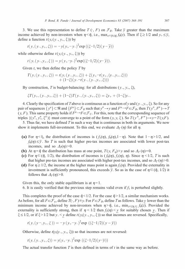
3. We use this representation to define T (·, F ) on FB. Take y greater than the maximumincome achieved by non-investors when ηb η, i.e., maxz∈[0,η] f0(z). Then if ξ≥1/2 and y+≤ y,define a function t ( y, ( y−, y+, ξ )) by

tð y; ð y−; yþ; nÞÞ ¼ − yð yþ− y−Þ2exp ððn−1=2Þð y − yÞÞwhile otherwise define t ( y, ( y−, y+, ξ )) by

t ð y; ð y−; yþ; n ÞÞ ¼ y ð yþ−y−Þ2expððn−1=2Þð y− yÞÞ:Given t, we then define the policy T by

Tð y; ð y−; yþ; nÞÞ ¼ tð y; ð y−; yþ; nÞÞ þ nð yþ−tð yþ; ðy−; yþ; nÞÞÞþ ð1−nÞð y−−tð y−; ð y−; yþ; nÞÞÞ

By construction, T is budget-balancing: for all distributions ( y−, y+, ξ),

nTð yþ; ð y−; yþ; nÞÞ þ ð1−nÞTð y−; ð y−; yþ; nÞÞ ¼ nyþ þ ð1−nÞy−:4. Clearly the specification of Tabove is continuous as a function of y and ( y−, y+, ξ). So for any

pair of sequences f yngoR and fFngoFB such that yn→y and FnYFaFB, then T ( y

n, Fn )→T( y, F ). This same property holds if FnYFaFU . For this, note that the corresponding sequence oftriples {( y−

n, y+n, ξn )} must converge to a point of the form ( y, y, ξ ). So T ( y n, F n )→y=T ( y,F ).

5. Thus far, we have defined T in such a way that is continuous in both its arguments. We nowshow it implements full-investment. To this end, we evaluate ΔT (η) for all η.

(a) For ηb η, the distribution of incomes is ( f1(η), f0(η),1−η). Note that 1−ηN1/2, andf0(η)≤ y . So T is such that higher pre-tax incomes are associated with lower post-taxincomes, and so ΔT(η)N0.

(b) At η= η the distribution has mass at one point, T ( y, Fη)≡y and so ΔT (η)=0.(c) For η∈ (η, 1/2), the distribution of incomes is ( f0(η), f1(η), η). Since η b1/2, T is such

that higher pre-tax incomes are associated with higher post-tax incomes, and so ΔT (η)N0.(d) For η≥1/2, the income at the higher mass point is again f1(η). Provided the externality in

investment is sufficiently pronounced, this exceeds y. So as in the case of η∈ (η, 1/2) itfollows that ΔT (η)N0.

Given this, the only stable equilibrium is at η=1.6. It is easily verified that the previous step remains valid even if f1 is perturbed slightly.

This completes the proof of the case ηb1/2. For the case ηN1/2, a similar mechanism works.As before, for all FaF u, define T(·, F )≡y. For FaFB, define T as follows. Take y_ lower than theminimum income achieved by non-investors when ηN η, i.e., minz∈[η,1] f0(z). Provided theexternality is sufficiently strong, then if η b 1/2 then f1(η) b y_ for suitably chosen y_ . Then ifξ≤1/2, or if ξN1/2 but y−b y_ define t ( y,( y−, y+, ξ )) so that incomes are reversed. Specifically,

tð y; ð y −; yþ; n ÞÞ ¼ − y ð yþ−y−Þ2exp ððn−1=2Þð y� yÞÞ

Otherwise, define t(y,(y−, y+, ξ)) so that incomes are not reversed:

tð y; ð y−; yþ; nÞÞ ¼ yð yþ−y−Þ2exp ððn−1=2Þð y− yÞÞThe actual transfer function T is then defined in terms of t in the same way as before.


Full-investment is implemented as follows. For ηb1/2 then there are 1−ηN1/2 at the highermass point, and the lower income is the investment income. Since by assumption this is less than y

¯,

incomes are reversed and investment yields more than non-investment.For η∈ [1/2,η), there are 1−η≤1/2 at the higher mass point; incomes are again reversed and

investment yields more than non-investment. Finally, if ηN η then there are ηN1/2 at the highermass point, and the lower income is the non-investment income. Since this is certainly above y

¯,

incomes are not reversed and investment yields more than non-investment. □

Appendix B. Basins of attraction in the linear example

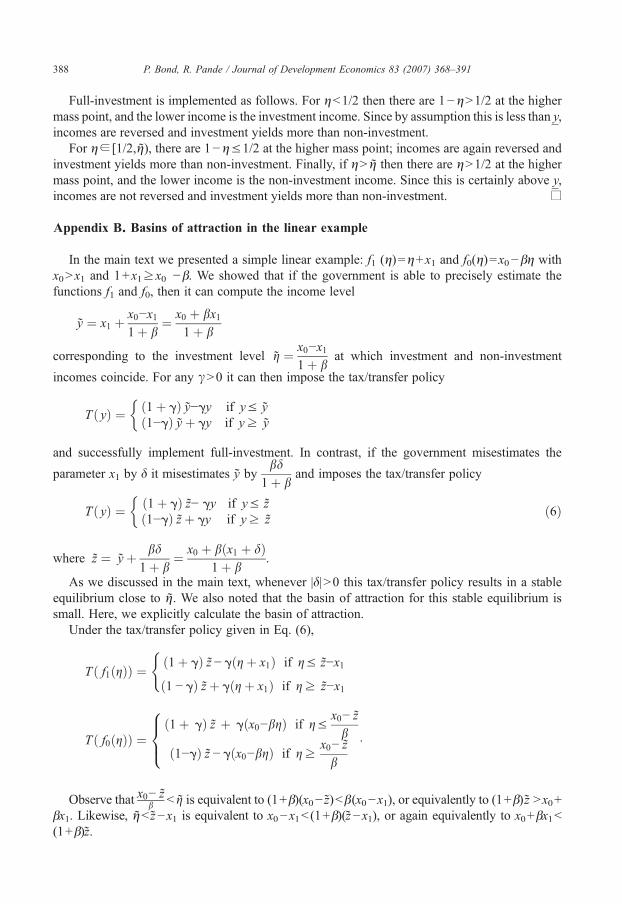
In the main text we presented a simple linear example: f1 (η)=η+x1 and f0(η)=x0−βη withx0Nx1 and 1+x1≥x0 −β. We showed that if the government is able to precisely estimate thefunctions f1 and f0, then it can compute the income level

y ¼ x1 þ x0−x11þ b

¼ x0 þ bx11þ b

corresponding to the investment level g ¼ x0−x11þ b

at which investment and non-investment

incomes coincide. For any γN0 it can then impose the tax/transfer policy

Tð yÞ ¼ ð1þ gÞ y−gy if y V yð1−gÞ yþ gy if yz y

�

and successfully implement full-investment. In contrast, if the government misestimates the

parameter x1 by δ it misestimates y bybd

1þ band imposes the tax/transfer policy

Tð yÞ ¼ ð1þ gÞ z− gy if y V zð1−gÞ zþ gy if yz z

�ð6Þ

where z ¼ yþ bd1þ b

¼ x0 þ bðx1 þ dÞ1þ b

.

As we discussed in the main text, whenever |δ|N0 this tax/transfer policy results in a stableequilibrium close to η. We also noted that the basin of attraction for this stable equilibrium issmall. Here, we explicitly calculate the basin of attraction.

Under the tax/transfer policy given in Eq. (6),

Tð f1ðgÞÞ ¼ ð1þ gÞ z− gðgþ x1Þ if g V z−x1

ð1 − gÞ zþ gðgþ x1Þ if gz z−x1

(

Tð f0ðgÞÞ ¼ð1þ gÞ z þ gðx0−bgÞ if g V

x0− zb

ð1−gÞ z − gðx0−bgÞ if gzx0− zb

:

8><>:

Observe that x0− zb b g is equivalent to (1+β)(x0− z)bβ(x0−x1), or equivalently to (1+β) z Nx0+

βx1. Likewise, ηb z−x1 is equivalent to x0−x1b (1+β)(z−x1), or again equivalently to x0+βx1b(1+β)z.


It follows that if δN0,

x0− zb

b g b z −x1;

while if δb0

z−x1b gb x0− z

b:

As such, when δN0 there are three subcases to consider:

If g V x0−zb ,then

DT ðgÞ ¼ gð2 z−ðgþ x1Þ − ðx0−bgÞÞ¼ gð2 z−x1−x0−ð1−bÞgÞ z g 2z−x1−x0−

ð1−bÞðx0−zÞb

� �¼ g

bðð2bþ ð1−bÞÞ z−bx1−ðbþ ð1−bÞÞx0Þ ¼ g

bðð1þ bÞ z−bx1−x0Þ ¼ g

bbd N 0:

If ga x0− zb ; z− x1

� �, then

DT ðgÞ ¼ gð−ðgþ x1Þ þ x0−bgÞ ¼ gðx0−x1−ð1þ bÞgÞ:

This is positive if and only if

g Vx0−x11þ b

¼ g:

Finally, if η≥ z−x1 then

DT ðgÞ ¼ gð−2 zþ ðgþ x1Þ þ ðx0−bgÞÞ ¼ gðx1 þ x0−2 zþ ð1−bÞgÞ

At η= z−x1 this is equal to

gðbx1 þ x0−ð1þ bÞ zÞ

which is negative. It is strictly increasing over the range, and is zero at

g ¼ 2 z−ðx1 þ x0Þ1−b

:

It follows that ΔT is negative if and only if

gax0−x11þ b

;2 z−ðx1 þ x0Þ

1−b

� �:


Consequently, there is a stable equilibrium at g ¼ x0−x11þ b

¼ g. The basin of attraction for this

equilibrium is 0; 2 z − ðx1þx0Þ1−b

h �. The righthand boundary of this interval lies a distance

2 z−ðx1 þ x0Þ1−b

−x0−x11þ b

¼ 2ðx0 þ bðx1 þ dÞÞ−ð1þ bÞðx1 þ x0Þ−ð1−bÞðx0−x1Þð1−bÞð1þ bÞ

¼ 2bdð1−bÞð1þ bÞ

away from the stable equilibrium η. That is, the distance from the newly created stableequilibrium to the right-hand boundary of its basin of attraction is proportional to δ, the size of thegovernment's misestimation of x1.

The analysis of the case in which δb0 is similar. In this case, δT is negative if and only if

ga2 z −ðx1 þ x0Þ

1−b;x0−x11þ b

� �;

and there is a stable equilibrium at2 z−ðx1 þ x0Þ

1−b . The basin of attraction is 0; x0−x11þb

h �; again, the

right hand boundary lies a distance2bd

ð1−bÞð1þ bÞ to the right of this equilibrium.

References

Abreu, Dilip, Matsushima, Hitoshi, 1992. Virtual implementation in iteratively undominated strategies: completeinformation. Econometrica 60 (5), 993–1008 (September).

Abreu, Dilip, Sen, Arunava, 1991. Virtual implementation in Nash equilibrium. Econometrica 59 (4), 997–1021 (July).Arya, Anil, Glover, Jonathan, Young, Richard, 1995. Virtual implementation in separable Bayesian environments using

simple mechanisms. Games and Economic Behavior 9, 127–138.Arya, Anil, Glover, Jonathan, Hughes, John S., 1997. Implementing coordinated team play. Journal of Economic Theory

74 (1), 218–232 (May).Battaglini, Marco, 2006. Joint production in teams. Journal of Economic Theory 130, 138–167.Becker, Gary S., Murphy, Kevin, Tamura, Robert, 1990. Human capital, fertility, and economic growth. Journal of Political

Economy 98 (5 Part 2), S12–S37.Besley, Timothy, Coate, Steve, 1992. Workfare versus welfare: incentive arguments for work requirements in poverty

alleviation programs. American Economic Review 82 (1), 249–261.Bhagwati, J., 1993. India's Economy: The Shackled Giant. Oxford University Press.Billingsley, Patrick, 1995. Probability and Measure. Wiley–Interscience.Chung, Kim-Sau, 1999. Affirmative action as an implementation problem. Working Paper.Cooper, Russell, 1999. Coordination Games: Complimentarities and Macroeconomics. Cambridge University Press.Gordon, H. Scott, 1954. The economic theory of a common-property resource: the fishery. Journal of Political Economy 62

(2), 124–142 (April).Guesnerie, Roger, 1995. A contribution to the pure theory of taxation. Cambridge.Hammond, Peter J., 1979. Straightforward individual incentive compatibility in large economies. Review of Economic

Studies 46 (2), 263–282 (April).Hirschman, A.O., 1957. The Strategy of Economic Development. Yale University Press, New Haven, CT.Hoff, Karla, 2000. Beyond Rosenstein–Rodan: The modern theory of coordination problems in development. Proceedings

of the Annual World Bank Conference on Development Economics.Holmström, Bengt, 1982. Moral hazard in teams. Bell Journal of Economics 13 (2), 324–340 (Autumn).


Krueger, A.O., 1997. Trade policy and economic development: how we learn. American Economic Review 87 (1), 1–22.Lanjouw, J.O., Lanjouw, Peter, 2001. The rural non-farm sector: issues and evidence from developing countries.

Agricultural Economics 26, 1–23.Legros, Patrick, Matthews, Steven A., 1993. Efficient and nearly-efficient partnerships. Review of Economic Studies 60

(3), 599–611 (July).Ma, Ching to, 1988. Unique implementation of incentive contracts with many agents. Review of Economic Studies 55,

555–571.Maskin, Eric, 1999. Nash equilibrium and welfare optimality. Review of Economic Studies 66, 23–38.Matsuyama, Kiminori, 1996. The Role of Government in East Asian Development: Comparative Institutional Analysis,

chapter Economic Development as Coordination Problems. Oxford University Press.Mirrlees, James A., 1971. An exploration in the theory of optimal income taxation. Review of Economic Studies 38,

175–208.Mookherjee, Dilip, 1984. Optimal incentive schemes with many agents. Review of Economic Studies 51 (3), 433–446

(July).Murphy, Kevin, Shleifer, Andrei, Vishny, Robert, 1989. Industrialization and the big push. Journal of Political Economy

97.Pigou, Arthur C. (Ed.), 1932. The economics of welfare. McMillan.Piketty, Thomas, 1993. Implementation of first-best allocations via generalized tax schedules. Journal of Economic Theory

61, 23–41.Porter, Ryan W., Shoham, Yoav, 2004. On cheating in sealed-bid auctions. Journal of Decision Support Systems 39,

41–54.Rai, Ashok S., 2002. Targeting the poor using community information. Journal of Development Economics 69,

71–84 (October).Ray, Debraj, 2000. What's new in development economics? The American Economist 441, 3–16.Rodrik, Dani, 1996. Coordination failures and government policy: a model with applications to East Asia and Eastern

Europe. Journal of International Economics 40 (1–2), 1–22 (February).Rosenstein-Rodan, Paul, 1943. Problems of industrialization of eastern and south eastern Europe. Economic Journal 53,

202–211 (June - September).Vickrey, William, 1961. Counterspeculation, auctions, and competitive sealed tenders. Journal of Finance 16 (1),

8–37 (March).

coordinating development: can income-based incentive schemes eliminate pareto inferior equilibria?

Documents