coordinating dynamic traffic-power systems under
TRANSCRIPT
HAL Id: hal-03249393https://hal.archives-ouvertes.fr/hal-03249393
Preprint submitted on 4 Jun 2021
HAL is a multi-disciplinary open accessarchive for the deposit and dissemination of sci-entific research documents, whether they are pub-lished or not. The documents may come fromteaching and research institutions in France orabroad, or from public or private research centers.
L’archive ouverte pluridisciplinaire HAL, estdestinée au dépôt et à la diffusion de documentsscientifiques de niveau recherche, publiés ou non,émanant des établissements d’enseignement et derecherche français ou étrangers, des laboratoirespublics ou privés.
Coordinating dynamic traffic-power systems underdecentralized, centralized, and information-sharing
decision environmentsHongping Wang, Adam F. Abdin, Yi-Ping Fang, Jakob Puchinger, Enrico Zio
To cite this version:Hongping Wang, Adam F. Abdin, Yi-Ping Fang, Jakob Puchinger, Enrico Zio. Coordinating dynamictraffic-power systems under decentralized, centralized, and information-sharing decision environments.2021. hal-03249393
Coordinating dynamic traffic-power systems underdecentralized, centralized, and information-sharing
decision environments
Hongping Wanga, Adam F.Abdina, Yi-Ping Fanga,∗, Jakob Puchingera,Enrico Ziob,c
aUniversité Paris-Saclay, CentraleSupélec, Laboratoire Génie Industriel, 3 rueJoliot-Curie, Gif-sur-Yvette, France.
bEnergy Department, Politecnico di Milano, 20156 Milano, Italy.cMines ParisTech, PSL Research University, CRC, Sophia Antipolis, France.
AbstractThis paper proposes a dynamic traffic-electric power network model to inves-tigate the interdependent electric power and road transport systems, whoseoperations are linked via the local marginal electricity price and the electricvehicles (EVs) charging demand. For the electric road network (ERN), anovel formulation based on the link transmission model is proposed to: 1)accommodate the critical features of EVs and fast charging stations (FCSs),such as EV with different driving ranges, initial states of charge of EVs,number of chargers and their charging power in a FCS; 2) explicitly modelthe charging process of EVs; 3) solve the optimal dynamic traffic assignmentproblem considering the mix of EVs and gasoline vehicles. For the economicoperation of the power distribution network (PDN), an alternating currentoptimal power flow model is solved to minimize the electricity expenditure.Moreover, we propose mathematical algorithms to model the decentralized,centralized and information-sharing decision-making environments, so thatthe operational difference and social benefits of coordinating traffic-power sys-tems can be compared. The proposed models and algorithms are applied toan illustrative traffic-power system. The results show that the decentralizeddecision-making always results in losses of operational cost and renewable in-tegration, compared to the centralized decision making; however, these losses
∗Corresponding author, Email address: [email protected]
Preprint submitted to Applied energy June 3, 2021
can be greatly mitigated by having ERN and PDN operators share informa-tion about the planned EV charging demand and the projected locationalmarginal electricity price.Keywords: Traffic-power system, Electric vehicles, Charging stations,Coordination, Decision-making environments, Link transmission model
1 Nomenclature
Indices
a index of links
t index of periods
s index of destinations
c index for classes of EVs
e index for energy levels of EVs
The electrified road network sets
A set of arcs
N set of nodes
A(i) (B(i)) set of links whose tail (head) node is i
AR set of source arcs
AS set of sink arcs
AG set of general arcs
AC set of charging arcs
T set of periods
Parameters
1∗Corresponding author: Email address: [email protected]
2

ϕ time value
peva charging power of charging link a
NCa(t) number of chargers at charging link a during period t
δ period length
La physical length of link a
kjam/qmax/vf jam density/ maximum flow/ free-flow speed
w backward shock-wave speed, w = qmax · vf/(qmax − kjam · vf )
αta average charging speed for charging link a during period t, αt
a =peva /(η · vf )
Ifa(t) inflow capacity of link a during period t
Ofa(t) outflow capacity of link a during period t
DGsa(t) cumulative gasoline vehicle travel demand between the entry of
origin link a and destination s at the end of period t
νa free-flow travel time on link a, νa = La/(δ · vf )
βa travel time required by the backward shock wave from the exitto the entry of link a, βa = La/(δ · w)
Variables
Ua(t) cumulative number of vehicles that enter link a by the end ofperiod t
Va(t) cumulative number of vehicles that leave link a by the end ofperiod t
UGa(t) cumulative number of GVs that enter link a by the end of in-terval t
UGsa(t) cumulative number of GVs that enter link a to destination s by
the end of period t
3

V Ga(t) cumulative number of GVs that leave link a by the end of inter-val t
V Gsa(t) cumulative number of GVs that leave link a to destination s by
the end of period t
UEs,ea,c(t) cumulative number of EVs of class c with energy level e that
enter link a to destination s by the end of period t
V Es,ea,c(t) cumulative number of EVs of class c with energy level e that
leave link a to destination s by the end of period t
xs,ea,c(t) occupancy of EVs of class c with energy level e at charging link
a during period t
xs,ea,c(t) occupancy of EVs of class c with the updated energy level e at
charging link a during period t
The electric vehicle sets
C set of electric vehicle classes
Parameters
Bc battery capacity of EVs of class c
Ec maximum energy level of the EVs of class c
η energy consumption of EVs
ρa energy levels required to traverse link a, ρa = La/η
Lmaxc driving range of EVs of class c, Lmax
c = Bc/η
Ec set of energy levels for the EVs belonging to class c, Ec =Lmaxc /(δ · vf )
The power network sets
PN set of buses
PL set of distribution lines
Γ(j) Successor set of bus j
4
Parameters
aj, bj Energy production cost coefficients at bus j
µ(t) Contract electricity price with the main grid in period t
prampj Ramp limits of generators at bus j
Variables
pgj (t) Active power generation at bus j during period t
pdcj (t) Charging load at bus j during period t
Pij(t) Active/Reactive power flowing from buses i to j during periodt
Acronym
EVs Electric Vehicles
FCSs Fast Charging Stations
ERN Electrified Road Network
PDN Power Distribution Network
1. Introduction
Electric vehicles (EVs) are increasingly deployed worldwide [1], due totheir potential contribution in reducing green house gas emission, increasedeconomic viability and convenience for the users. However, this brings newchallenges to both the transportation and power systems. EV drivers needto consider the charging cost and time at different charging stations, whenplanning their trips. Traffic patterns are affected by the electricity price andthe locations of fast charging stations (FCSs). On the one hand, the spatialand temporal charging demand resulting from the EVs charging patternsimpacts the distribution of power flow, which challenges the operation ofthe existing power systems. On the other hand, this provides opportunitiesto efficiently operate power systems through vehicle-to-grid exchanges whichcould stabilize the power flow under the conditions of increased integration ofrenewable energy. In this setting, the power systems and the electrified road
5
networks (ERNs) interact with each other through the dynamics of electricityprice and charging demand. Such interplay brings challenges to control andoperate the two systems, but also brings opportunities to promote integrationand communication between each other.
Investigating how to model, operate and control the coupled ERNs andpower systems considering EV charging has gained attention in recent years[2, 3, 4]. Some of the main challenges addressed in the literature are how toproperly model the physical features of the coupled transportation systemsand power systems, as well as, modeling EVs and EVs supply equipment.
Some studies only consider the ERNs, ignoring the technical constraintscoming from the power systems. Their objectives are mainly of optimizing al-location of FCSs [5, 6, 7], charging navigation [8] and routing [9, 10], as well assimulating coordinated and uncoordinated charging modes [11]. Some stud-ies, instead, only consider detailed power systems modeling including EVscharging load, without considering realistic features of ERNs. Some of thetopics considered can be summarized as: 1) Investigating the impacts of EVson power systems in terms of safety [12], reliability [13], normal operation[14], among others. 2) Long term planning problems [15], e.g., optimizingthe allocation of smart grid components and charging stations [16, 17]; re-inforcing power systems capacity to enable the massive deployment of solarphotovoltaics, electric heat pumps and EVs [18], among others. 3) Coordi-nating EVs charging [19], such as, minimizing the number of coordinated EVsto mitigate voltage unbalance [20]; coordinating EVs charging while main-taining the voltage deviation within acceptable power quality limits [21];managing day-ahead electricity procurement and real-time EVs charging tominimize the total operating cost [22]. In the majority of cases, the spa-tial and temporal charging demand are required to be estimated statisticallyfrom existing data, which is however difficult to access.
Other studies consider the coupled power systems and ERNs, and investi-gate the interdependency between the two systems [23]. Several frameworks[24, 25, 26] have been proposed to model the interaction of traffic-power sys-tems, wherein in most models the traffic and power flow interact with eachother through electricity price, charging load and traffic toll. In this paper,we consider that the traffic flow within the ERNs and the power flow areinterdependent through the charging demand at each FCS and the associ-ated locational marginal price (LMP). Within this interaction process, froman ERN operator’s perspective, the dynamic electricity price (i.e., LMP) andthe capacity of FCSs are important parameters. The former is obtained from
6

power systems and the latter is a key physical feature of an ERN. Both caninfluence the route choice of EV drivers and non-EV drivers, since EVs driversshare the limited capacity of a FCS, and EVs and non-EVs drivers share thelimited capacities of roads. Therefore, traffic flow patterns are affected byboth factors and, further impact the distribution of charging demand. Froma power system operator’s perspective, the accurate data of the spatial andtemporal charging demand from an ERN can help to manage the electric-ity production and balance the power flow of the systems. The spatial andtemporal charging loads affect the power flow distribution subject to powersystem constraints, such as limitation of the grid and generator capacities,as well as ramp limits of generators. The power flow distribution, in return,influences the LMP, which would further affect traffic flow distribution. Inthis way, the ERN and power system interact with each other and both FCSsand EVs play critical roles in this interdependent traffic-power systems. Theformer is the interface connecting the ERN and power system, and the lat-ter acts as the power prompting the interplay between traffic and powerflow. Therefore, properly modeling the detailed physical features of EVs andFCSs is important to adequately study the interaction between the ERN andthe power system. Here, we list some of the critical features that need tobe modeled when investigating the interdependency of traffic-power systemsand how they have been considered in the literature. A detailed comparisonof these features in the literature is listed in Table 1.
Dynamics (feature of the coupled systems): A dynamic traffic-powersystem model is required due to: 1) the spatial and temporal nature of EVs;2) the time-varying evolution of traffic flow; 3) the ramp limits of powergenerators. Most existing studies only considered a static model [27, 28,29, 30, 31], whereas recently increasing attention has been paid to modelingdynamic [32, 33] or semi-dynamic [34] traffic-power systems.
Charging time (feature of EV): It is part of the travel time cost, whenthe time value is considered. Refs. [30, 31] assumed that all EVs, had (A1)the same exogenously given fixed charging time. This assumption is markedas (A1).
Charging demand (feature of EV): It influences the charging cost forEV drivers, and influences power production as well as power flow distribu-tion. Refs. [28, 30, 31, 29] assumed all EVs had (A2) the same exogenouslygiven fixed charging demand; Refs. [32, 34, 29] assumed the charging demandwas (A3) only related to traffic flow through the FCSs without consideringthe real charging needs. It could cause the EVs to charge multiple times with-
7
out considering the remaining battery capacity leading to an overestimationof the charging demand.
Driving range/Battery capacity (feature of EV): It influences thenumber of times an EV has to recharge during a trip.
Initial state of charge (SoC) (feature of EV): It influences whether itis required to recharge an EV at the beginning of the time horizon. If ithas, the initial SoC of an EV influences which FCSs this EV is able to reachwithout running out of battery. Ref. [28] assumed (A4) an EV was able toreach any FCS. This assumption may result in the assigned charging pointto be beyond the remaining driving range of an EV.
Mix of gasoline vehicles (GVs) (feature of an ERN): EVs and GVscompete for the limited road capacity.
Capacity of FCSs (feature of an ERN): EVs compete for the limitedcharging capacities at FCSs.
Additionally, several decision-making environments considered for co-operations of traffic-power systems are summarized in Table 1. Centralizeddecision-making environments describe a situation where there is a singleoperator who controls both ERNs and power systems in a fully integratedmanner. Their objectives usually lead to a social optimum. Information−sharing decision-making environments describe a situation where ERNs andpower systems operate independently, but they can share their operationplans at the beginning of each time step [32] or at the beginning of the timehorizon [28, 30, 33]. Their own plans do not need to change according to thereceived information. They also can exchange their plans for any numberof rounds. The sufficient information-sharing in Table 1 means that boththe ERN operator and the power system operator share their informationuntil converging (e.g., the changes of traffic flow pattern and charging priceare smaller than a threshold [28]) or meeting the maximum iteration rounds.Refs. [28, 30, 32] showed that, under the sufficient information-sharing situ-ation, the solution approximates to an equilibrium between ERNs and powersystems. Furthermore, Ref. [33] has proved that the social optimum is ageneral equilibrium if LMP is used in power systems, where the power sys-tem operator is a nonprofit one whose objective is to balance the electricitysupply and demand under technical security constraints. Since the powersystem operator is welfare-minded, it can steer a selfish ERN operator to-wards the social optimum. More discussions are detailed in Refs. [33]. Asshown in Table 1, a systematic analysis for the interaction of traffic-powersystems under different decision-making environments is missing.
8

Table 1: Summary of considered factors in relevant literatures
references decision-making environments dynamics EV features ERNs features
chargingtime
chargingdemand
drivingrange
initialSoC GVs capacity
of FCSs
[35] centralized × (A3) × × × ×[32] limited information-sharing × (A3) × × × [36] centralized (A1) (A2) × × × [34] centralized × (A3) × × × ×[27] centralized × × ×[28] sufficient information-sharing × (A2) × (A4) [29] centralized × × (A3) × [30] sufficient information-sharing × (A1) (A2) × × [31] centralized × (A1) (A2) × ×
To fill the research gaps mentioned above, this paper proposes a dynamictraffic-power system model and investigates the coordination of traffic-powersystems under centralized, decentralized and information-sharing decision-making environments.
The main contributions of the paper are summarized as follows:1) We propose a novel dynamic traffic-power system model, which is able
to capture the spatial-temporal traffic flow evolution and charging demand.Dynamic models can provide more accurate charging load information com-pared to static ones.
2) Within the proposed model, an electric link transmission model (eLTM)is proposed to solve the system optimal dynamic traffic assignment (SO-DTA) problem. The critical features of EVs and ERNs, summarized in Table1, are thoroughly considered. Moreover, the proposed model also considersthe different classes of EVs with different driving ranges, chargers with dif-ferent charging powers in a FCS and the charging process of EVs. Theseextensions allow the model to be used in various applications and at differ-ent granularities.
3) This paper systematically investigates the operation of traffic-powersystems under centralized, decentralized and information-sharing decision-making environments. The corresponding objective functions under differentdecision-making environments are formulated. An iterative algorithm is pro-posed to solve the centralized optimization problem. We compare the threeenvironments in terms of the charging congestion level at FCSs, chargingprice, charging demand, integration of renewable energy, among others.
The remainder of the article is structured as follows. Section 2 developsthe traffic-power system model. Section 3 describes decentralized, centralized
9

and information-sharing decision-making environments. Section 4 illustratesa numerical example to show the application of the proposed model and com-pares the solutions under different decision-making environments. Finally,Section 5 provides some concluding remarks and future research directions.
2. Coupled traffic-power system
2.1. Link transmission model based system optimal dynamic traffic assign-ment problem
A road network with multiple sources (origins) and sinks (destinations)is denoted as G(N ,A), where N and A are the sets of nodes and links,respectively. All links (nodes) in the road network are classified into threetypes: source, sink and general links (nodes). Within the road network, eachsource (sink) node attaches only one source (sink) link, and each source (sink)link connects to only one source (sink) node. NR (resp. NS) and AR (AS)denote the set of source (sink) nodes and source (sink) links, respectively.All source (sink) links are dummy of length zero and infinite outflow, inflowand storage capacities. For SO-DTA problems, the outflow capacity of allsink links are assumed to be 0, which means that all vehicles are collectedupon their arrival. The time horizon H is discretized into a finite set ofperiods T = t = 1, 2, · · · , T. T is calculated according to T = H/δ, whereδ is the period length. The period length should be equal to or smaller thanthe smallest link travel time so that vehicles take at least one time unit totraverse a link [37].
A triangular fundamental diagram is used in the link transmission model(LTM) [37, 38], which is an approximation and describes a macroscopic prop-erty of roads considering the number of lanes, weather conditions, speed lim-its, among others [37]. The diagram is defined by three parameters: a jamdensity (kjam), a maximum flow (qmax) and a fixed-free flow speed (vf ). Thebackward shock-wave speed w can be obtained by w = qmax · vf/(qmax −kjam · vf ). The LTM updates the traffic flow evolution by calculating thecumulative number of vehicles at the entry and exit of each link in eachperiod.
The Newell’s simplified theory is used in LTM to calculate sending Sa(t)and receiving Ra(t) capacities of link a:
Sa(t) = minUa(t− νa)− Va(t− 1), Ofa(t) (1a)
10

Ra(t) = minVa(t− βa) + La · kjam − Ua(t− 1), Ifa(t) (1b)where Ua(t) (Va(t)) denotes the cumulative number of vehicles that enter(leave) link a by the end of period t, respectively. Ifa(t) and Ofa(t) arethe inflow capacity at the entering point and outflow capacity at the leavingpoint of link a during period t. They can be obtained by δ · qmax at thecorresponding location and period. La is the length of link a. νa is the free-flow travel time on link a and βa is the travel time required by the backwardshock wave from the exit to the entry of link a. They can be obtained byνa = La/(δ · vf ) and βa = La/(δ · w), respectively.
The inflow and outflow of link a during interval t are constrained by itscorresponding sending and receiving capacities, respectively:
Ua(t)− Ua(t− 1) ≤ Ra(t),∀a ∈ A, t ∈ T (2a)
Va(t)− Va(t− 1) ≤ Sa(t),∀a ∈ A, t ∈ T (2b)In the LTM-based SO-DTA problem, the different classes of vehicles are
not distinguished. Thus, we have:
Ua(t) =∑s∈NS
UGsa(t),∀a ∈ A, t ∈ T (3a)
Va(t) =∑s∈NS
V Gsa(t), ∀a ∈ A, t ∈ T (3b)
where UGsa(t)(V Gs
a(t)) denotes the cumulative number of gasoline vehiclesthat enter(leave) link a to destination s by the end of period t.
Substituting Eqs. (1) and (3) into the inequalities in Eq. (2), the linearLTM-based flow constraints are obtained as follows:∑
s∈NS
V Gsa(t) ≤
∑s∈NS
UGsa(t− νa),∀a ∈ A, t ∈ T (4)
∑s∈NS
[V Gsa(t)− V Gs
a(t− 1)] ≤ Ofa(t),∀a ∈ A, t ∈ T (5)
∑s∈NS
UGsa(t) ≤
∑s∈NS
V Gsa(t− βa) + La · kjam,∀a ∈ A, t ∈ T (6)
11

∑s∈NS
[UGsa(t)− UGs
a(t− 1)] ≤ Ifa(t), ∀a ∈ A, t ∈ T (7)
The cumulative outflow to destination s should be constrained by thecumulative inflow to the same destination on link a:
V Gsa(t) ≤ UGs
a(t− νa),∀a ∈ A, t ∈ T (8)
The traffic demand is satisfied by letting the cumulative inflows of sourcelinks equal to the cumulative demands:
UGsa(t) = DGs
a(t), ∀a ∈ AR, ∀s ∈ NS, t ∈ T (9)
where DGsa(t) is the cumulative gasoline vehicle travel demand between the
entry of origin link a and destination s at the end of period t.In the LTM model, the inflow and outflow of a general node should be
restricted by the following flow conservation constraints:∑a∈B(i)
V Gsa(t) =
∑b∈A(i)
UGsa(t),∀i ∈ N /NR,NS,∀s ∈ NS, t ∈ T (10)
where A(i) (B(i)) represents the set of links whose tail (head) node is i.The cumulative flows should be nonnegative and nondecreasing :
V Gsa(t)− V Gs
a(t− 1) ≥ 0,∀a ∈ A, ∀s ∈ NS, t ∈ T (11)
UGsa(t)− UGs
a(t− 1) ≥ 0,∀a ∈ A,∀s ∈ NS, t ∈ T (12)The following constraints force the initial cumulative flows to be 0:
UGsa(0) = V Gs
a(0) = 0,∀a ∈ A,∀s ∈ NS (13)
The objective of the LTM-based SO-DTA problem is to minimize thetotal travel time of all vehicles. The total travel time is calculated by thetotal presence time of all vehicles on all links during the whole time horizon.The LTM-based SO-DTA problem [38] is formulated as follows:
minx∈Ω
∑a∈A/AS
∑s∈NS
∑t∈T
δ[UGsa(t)− V Gs
a(t)] (14)
where Ω = x| s.t. (4)− (13).
12
2.2. eLTM-based SO-DTA problemThe existing LTM-based SO-DTA model is not able to describe the new
features related to the EVs, such as the driving range of EVs and the capacityof FCSs. To overcome this shortcoming, an eLTM-based SO-DTA modelis proposed to minimize the total cost for all vehicles considering the EVsdriving ranges, FCS capacities, charging costs, among others.
The assumptions in this model are:(1) An EV charges the minimum en-route to ensure the shortest travel
time. The SoC after charging (original SoC plus the charged electricity)should ensure that the EV can reach the destination or the next FCS. Thisassumption is coherent with the objective function of the proposed model,which is to minimize the total cost. Other phenomena, e.g., the EVs onlyleave FCSs after being fully charged or 80% charged, can be easily incor-porated by adding constraints on FCSs. As for the heterogeneous chargingpreferences of EV drivers, their consideration is not within the scope of thispaper.
(2) The electricity consumed by an EV is linearly related to the distancetraveled. The electricity amount charged by an EV is linearly related to thecharging time. All EV batteries have the same energy consumption efficiency,similar to Ref. [39].
(3) The electricity consumed by the in-vehicle equipment, such as air con-ditioners and lights, is neglected. When EVs stop, no electricity is consumed.
In order to track the SoC of EVs, the model accounts for different energylevels to describe the real-time SoC for each EV. Given a certain class of EVdenoted as c, its battery capacity is Bc kWh and the energy consumptionefficiency is η kWh/mile: then, the mileage of this class EV is Bc/η = Lmax
c
miles. One energy level (EL) is defined to be equal to δ · vf miles. Therefore,the maximum EL of EV of class c is calculated by Ec = Lmax
c /(δ · vf ).Assuming that there are C EV classes represented as C = E1, E2, · · · , EC,each element in set C is a set, which contains the energy levels that EV ofclass c could have, denoted as Ec = 1, 2, · · · , Ec.
To describe the FCS in the physical road network, dummy charging linksAC are originally defined in the eLTM-based model. A FCS is modeled byone or several charging links, represented by arcs having the same origin anddestination, as shown in Fig. 1. Chargers with different charging speeds arerepresented by different charging links. Parameter αt
a represents the averagecharging speed for each charging link a during period t, which translates
13
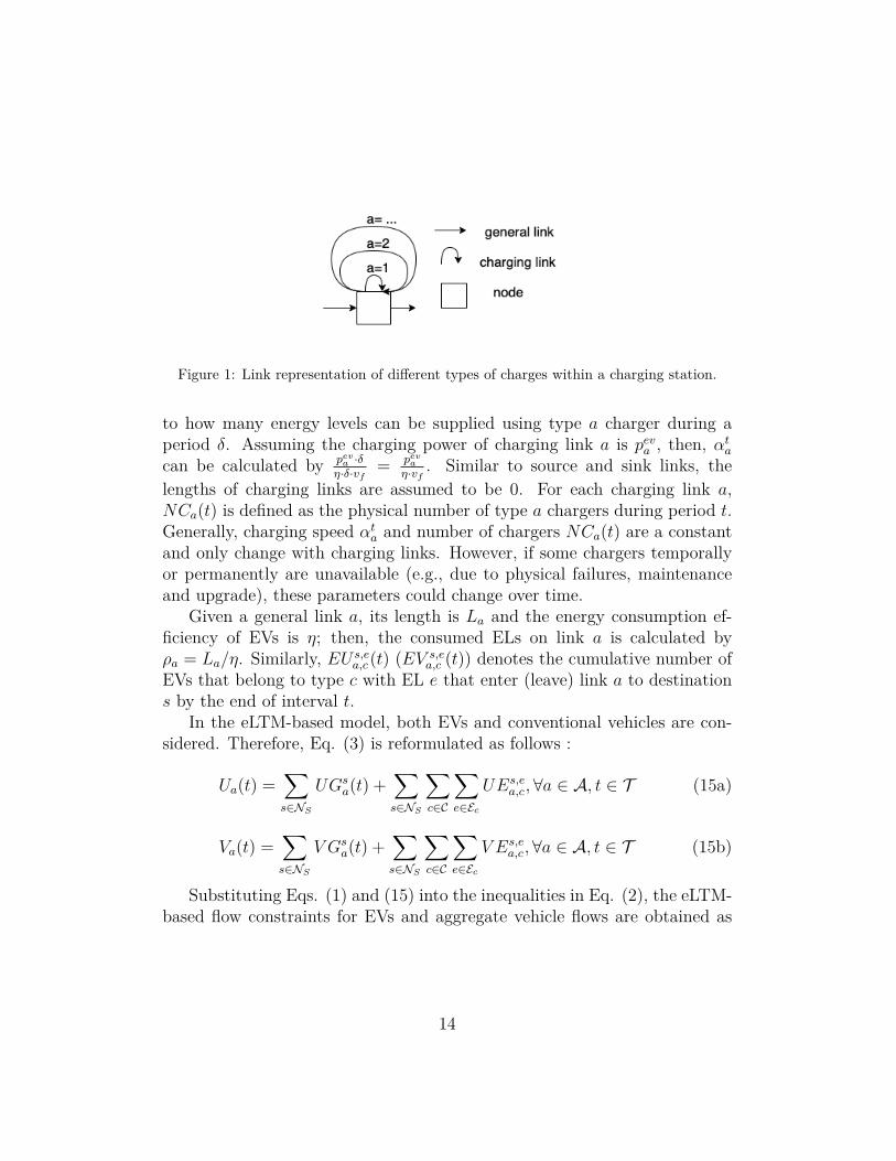
Figure 1: Link representation of different types of charges within a charging station.
to how many energy levels can be supplied using type a charger during aperiod δ. Assuming the charging power of charging link a is peva , then, αt
a
can be calculated by peva ·δη·δ·vf
= pevaη·vf
. Similar to source and sink links, thelengths of charging links are assumed to be 0. For each charging link a,NCa(t) is defined as the physical number of type a chargers during period t.Generally, charging speed αt
a and number of chargers NCa(t) are a constantand only change with charging links. However, if some chargers temporallyor permanently are unavailable (e.g., due to physical failures, maintenanceand upgrade), these parameters could change over time.
Given a general link a, its length is La and the energy consumption ef-ficiency of EVs is η; then, the consumed ELs on link a is calculated byρa = La/η. Similarly, EU s,e
a,c (t) (EV s,ea,c (t)) denotes the cumulative number of
EVs that belong to type c with EL e that enter (leave) link a to destinations by the end of interval t.
In the eLTM-based model, both EVs and conventional vehicles are con-sidered. Therefore, Eq. (3) is reformulated as follows :
Ua(t) =∑s∈NS
UGsa(t) +
∑s∈NS
∑c∈C
∑e∈Ec
UEs,ea,c, ∀a ∈ A, t ∈ T (15a)
Va(t) =∑s∈NS
V Gsa(t) +
∑s∈NS
∑c∈C
∑e∈Ec
V Es,ea,c, ∀a ∈ A, t ∈ T (15b)
Substituting Eqs. (1) and (15) into the inequalities in Eq. (2), the eLTM-based flow constraints for EVs and aggregate vehicle flows are obtained as
14

follows:
V Es,ea,c(t) ≤ UEs,e+ρa
a,c (t− νa),∀a ∈ A\AC,∀s ∈ NS,∀c ∈ C, e ∈ Ec ∩ e ≤ Ec − ρa, t ∈ T
(16a)
V Es,ea,c(t) = 0,∀a ∈ A\AC,
∀s ∈ NS, ∀c ∈ C, e ∈ Ec ∩ e > Ec − ρa, t ∈ T(16b)∑
s∈NS
[V Gsa(t)− V Gs
a(t− 1)] +∑s∈NS
∑c∈C
∑e∈Ec
[V Es,ea,c(t)− V Es,e
a,c(t− 1)]
≤ Ofa(t),∀a ∈ A\AC, t ∈ T(17)
∑s∈NS
∑c∈C
∑e∈Ec
[UEs,ea,c(t)− V Es,e
a,c(t− βa)]+∑s∈NS
[UGsa(t)− V Gs
a(t− βa)] ≤ Lakjam,∀a ∈ A\AC, t ∈ T(18)
∑s∈NS
[UGsa(t)− UGs
a(t− 1)]+∑s∈NS
∑c∈C
∑e∈Ec
[UEsa(t)− UEs
a(t− 1)] ≤ Ifa(t),∀a ∈ A\AC, t ∈ T(19)
Eq. (16a) guarantees that the outflow should be less than or equal to theinflow and that the consumed ELs are deducted after EVs traversed thecorresponding links. Eq. (16b) ensures that EV ELs are less than theirmaximum ELs. Eqs. (17) - (19) are same as Eqs. (5) - (7). Eqs. (17)and (19) constrain the outflow and inflow to be less than or equal to theiroutflow and inflow capacities, respectively. Eq. (18) states that the numberof vehicles on link a should be less than or equal to the maximum number ofvehicles that can be contained on this link.
Eq. (20) ensures that traffic demand of EVs should also be satisfied:
UEs,ea,c(t) = DEs,e
a,c(t), ∀a ∈ AR, ∀s ∈ NS,∀c ∈ C,∀e ∈ Ec, t ∈ T (20)
Similar to Eq. (10), the flow conservation law should also be followed by
15
EVs: ∑a∈B(i)
V Es,ea,c(t) =
∑b∈A(i)
UEs,ea,c(t),
∀i ∈ N /NR,NS, ∀s ∈ NS,∀c ∈ C,∀e ∈ Ec, t ∈ T(21)
2.2.1. Modeling EV charging processTo model the charging process, intermediate variables xs,e
a,s(t) and xs,ea,s(t)
are defined as the number of EVs before and after their ELs have been up-dated on charging link a. The occupancy xs,e
a,s(t) on a charging link is calcu-lated by the occupancy plus new inflow minus outflow during the previousperiod, as shown in Eq. (22):
xs,ea,s(t) = xs,e
a,s(t− 1) + [UEs,ea,c(t− 1)− UEs,e
a,c(t− 2)]−[V Es,e
a,c(t− 1)− V Es,ea,c(t− 2)],
∀a ∈ AC ,∀s ∈ NS, ∀c ∈ C,∀e ∈ Ec, t ∈ T(22)
Furthermore, the following equations describe the process of updating theELs on charging links:
xs,Eca,c (t) =
αta∑
l=0
xs,Ec−la,c (t), ∀a ∈ AC ,∀s ∈ NS,∀c ∈ C,∀t ∈ T (23a)
xs,ea,c(t) = xs,e−αt
aa,c (t), ∀a ∈ AC ,∀s ∈ NS,∀c ∈ C,∀e ∈ αt
a ≤ e < Ec,∀t ∈ T(23b)
xs,ea,c(t) = 0,∀a ∈ AC ,∀s ∈ NS,∀c ∈ C,∀e ∈ e < αt
a,∀t ∈ T (23c)
Eqs. (23a) and (23c) constrain the upper and lower bounds of the updatedELs. Eqs. (23b) describe the process of linear increase in ELs. Eq. (23a)states that if the ELs of EVs before being updated belong to [Ec − αt
a, Ec],their energy levels are approximately updated as the maximum EL Ec of EVof class c after one period. Eq. (23b) states that if the ELs of EVs are within[0, Ec − αt
a) before being updated, they increase αta ELs after one period.
The updated ELs are within [αta ≤ e < Ec). Eq. (23c) ensures that no EVs’
ELs are less than αta level after being charged for one period. Therefore, if
the updated ELs are smaller than αta, they are forced to be 0. Note that the
number of EVs on charging links are conserved before and after the ELs of
16

the EVs are updated, i.e.,∑
e xs,ea,c(t) =
∑e x
s,ea,c(t).
Additionally, the outflow disaggregated by each EL on charging link ashould be less than its occupancy, as formulated in Eq. (24):
V Es,ea,c(t)− V Es,e
a,c(t− 1) ≤ xs,ea,c(t),∀a ∈ AC , ∀s ∈ NS,∀c ∈ C,∀e ∈ Ec,∀t ∈ T
(24)
Eq. (25) limits the number of EVs on charging link a to its maximum numberof chargers:∑
s∈NS
∑c∈C
∑e∈Ec
[UEs,ea,c(t)− V Es,e
a,c(t)] ≤ NCa(t), ∀a ∈ AC ,∀t ∈ T (25)
Moreover, Eqs. (26) - (27) ensure that the cumulative EV flows are nonneg-ative and nondecreasing:
V Es,ea,c(t)− V Es,e
a,c(t− 1) ≥ 0,∀a ∈ A,∀s ∈ NS,∀c ∈ C,∀e ∈ Ec, t ∈ T (26)
UEs,ea,c(t)− UEs,e
a,c(t− 1) ≥ 0,∀a ∈ A,∀s ∈ NS, ∀c ∈ C,∀e ∈ Ec, t ∈ T (27)
Similarly, the occupancies on charging links is nonnegative, as described inEq. (28):
xs,ea,c(t) ≥ 0, xs,e
a,c(t) ≥ 0,∀a ∈ AC ,∀s ∈ NS,∀c ∈ C,∀e ∈ Ec, t ∈ T (28)
The occupancies on charging links and the cumulative EV flows are initializedto be 0, as formulated in Eq. (29):
UEs,ea,c(0) = V Es,e
a,c(0) = 0,∀a ∈ A,∀s ∈ NS,∀c ∈ C,∀e ∈ Ec (29)
As for the LTM-based SO-DTA problem, the objective of the eLTM-basedSO-DTA problem is to minimize the total travel time, including the chargingtime of EVs. The problem is formulated as:
miny∈Ψ
∑s∈NS
∑t∈T
∑a∈A/AC ,AS
δ[UGsa(t)− V Gs
a(t)]
+∑s∈NS
∑t∈T
∑a∈A/AS
∑c∈C
∑e∈Ec
δ[UEs,ea,c(t)− V Es,e
a,c(t)](30)
17
where Ψ = y| s.t. (8) − (13) and (16) − (29). It should be noted thatfor all a in constraints (8)-(13) its domain does not include AC . It meansconventional vehicles never go into charging links.
2.3. Power distribution network (PDN) modelWe consider a radial PDN GP (PN ,PL), where PN and PL represent the
sets of buses and distribution branches, respectively. In a radial network, eachbus is attached to a unique predecessor bus and the number of buses equalsto that of branches, which excludes a slack bus. Slack bus is indexed as 0.The successor set of bus j is denoted as Γ(j) = ∀k : (j, k) ∈ PL. The powersystem model in Ref. [28] is employed in this paper. We additionally addconstraint (31) to limit the generator ramp between two successive periods:
−prampj ≤ pgj (t)− pgj (t− 1) ≤ pramp
j ,∀j ∈ PN ,∀t ∈ T (31)
where pgj is the active power generation in period t and prampj is the ramp
limits of generators at bus j.The EV charging load in Ref. [28] is calculated by the static traffic flow
passing charging stations and the energy demand of each EV is assumed tobe fixed. In our paper, the charging load during each period is calculated bythe number of EVs stoping in charging links. The energy demand of each EVis consistent with assumption (1) in subsection 2.2. Thus, the EV chargingload in Eq. (28) in Ref. [28] is replaced by the following equation:
pdcj (t) =∑
a∈M(j)
∑s∈NS
∑c∈C
∑e∈Ec
peva [UEs,ea,c(t)− V Es,e
a,c(t)] (32)
where M(j) is a mapping from bus set PN to charging links set AC , whichspecifies the connection between buses in a power system and charging linksin a road network. N(a) is a reverse mapping of M(j), which maps charginglinks set to the bus set. The LMP at each bus is denoted as λt
j. The chargingprice at charging link a can be obtained by λt
N(a).To clearly describe the PDN model here, we detail the objective function
used. The objective of the PDN operator is to minimize the total energyproduction costs. The optimal power flow problem is defined as P1:
minz∈Φ
∑t∈T
∑j∈PN
[aj(pgj (t))
2 + bjpgj (t)] +
∑t∈T
∑k∈Γ(0)
µ(t)P0k(t) (33)
18
Φ = z| s.t. (31)− (32), and (24)− (34) in Ref. [24] (34)
where aj and bj are the production cost coefficients at bus j. P0k is the activepower flow from main grid to bus k. The first term is the production cost ofthe local generators and the second term is the cost for purchasing electricityfrom the main grid. µ(t) is the contract energy price during period t withthe main grid.
3. Decision environments
In this section, three decision-making environments are considered foroperating the traffic-power systems, which may arise when different bene-ficiaries coordinate the interdependent infrastructures. Analyzing differentdecision-making environments allows us to compare their operational andsocially beneficial difference. The value of sharing information also can bestudied.
3.1. Decentralized decision environmentsIn current practice, individual infrastructure systems such as ERNs and
PDNs often determine their operation in an independent, decentralized man-ner with little information exchange among them.
For the ERN sector, we adopt a system optimum model where the objec-tive is to minimize the total travel cost through dynamic traffic assignment.The total travel cost includes the driving time cost of both EVs and GVs,charging time cost of EVs and charging cost of EVs. This optimal traffic flowproblem P2 is formulated as follows:
miny∈Ψ
∑s∈NS
∑t∈T
∑a∈A/AC ,AS
ϕδ[UGsa(t)− V Gs
a(t)]
+∑s∈NS
∑t∈T
∑a∈A/AS
∑c∈C
∑e∈Ec
ϕδ[UEs,ea,c(t)− V Es,e
a,c(t)]+∑s∈NS
∑t∈T
∑c∈C
∑e∈Ec
∑a∈AC
λtN(a)p
eva δ[UEs,e
a,c(t)− V Es,ea,c(t)]
(35)
subject to constraints (8)-(13) and (16)-(29), where ϕ is the time value.Since the ERN operator does not know the real-time electricity price λt
N(a)
beforehand, we assume that an estimated fixed charging price is used for the
19

(a) Procedures of decentralizeddecision-making environment
(b) Procedures of information-sharing decision-making environ-ment
Figure 2: Procedures of decentralized and information-sharing decision-making environ-ments. CD: Charging demand of EVs; LMP: locational marginal price.
operator. For the PDN, it is assumed that the operator only knows the real-time charging demand and the demand in the future time periods is unknown.Thus, P1 is solved for each independent period for a total of T times. Themain process is shown in Fig. 2(a). At the beginning, the estimated chargingprice (LMP) for the ERN operator is used to solve P1. Then, in each period,the PDN operator receives the real-time charging demand from each FCS.Based on the real-time power demand, the operator solves P2 to obtain theoptimal power flow pattern z and the corresponding actual LMP in eachperiod. Note that this price dose not change the traffic assignment solutions.In the end, the actual charging cost for the ERN operator can be calculatedby the actual LMP.
3.2. Centralized decision environmentsThe centralized decision-making environment assumes that there is a cen-
tralized operator that coordinates both the ERNs and the PDNs to minimizethe total cost of the two systems. It means that ERNs and PDNs fully inte-grate with each other, although this may lead to sacrifice their own benefitsfrom an independent system’s perspective. This situation may be ideal, butthe results can serve as a benchmark to understand and analyze the best
20
possible coordination between ERNs and PDNs. This environment can beexpressed as the following optimization problem:
miny,z∈Ψ,Φ
∑s∈NS
∑t∈T
∑a∈A/AC ,AS
ϕδ[UGsa(t)− V Gs
a(t)]
+∑s∈NS
∑t∈T
∑a∈A/AS
∑c∈C
∑e∈Ec
ϕδ[UEs,ea,c(t)− V Es,e
a,c(t)]+∑s∈NS
∑t∈T
∑c∈C
∑e∈Ec
∑a∈AC
λtN(a)p
eva δ[UEs,e
a,c(t)− V Es,ea,c(t)]
+∑t∈T
∑j∈PN
[aj(pgj (t))
2 + bjpgj (t)] +
∑t∈T
∑k∈Γ(0)
µ(t)P0k(t)
(36)
subject to constraints (8)-(13), (16)-(29) and (34).Since variables λt
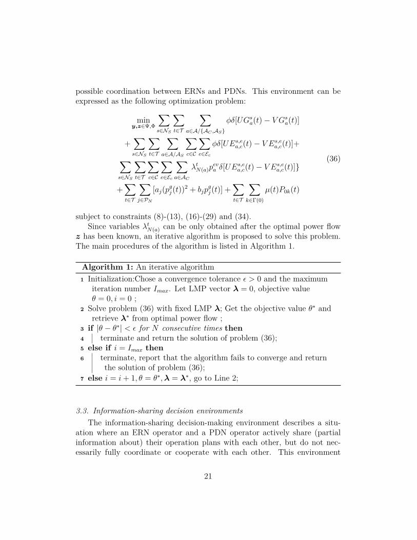
N(a) can be only obtained after the optimal power flowz has been known, an iterative algorithm is proposed to solve this problem.The main procedures of the algorithm is listed in Algorithm 1.
Algorithm 1: An iterative algorithm1 Initialization:Chose a convergence tolerance ϵ > 0 and the maximum
iteration number Imax. Let LMP vector λ = 0, objective valueθ = 0, i = 0 ;
2 Solve problem (36) with fixed LMP λ; Get the objective value θ∗ andretrieve λ∗ from optimal power flow ;
3 if |θ − θ∗| < ϵ for N consecutive times then4 terminate and return the solution of problem (36);5 else if i = Imax then6 terminate, report that the algorithm fails to converge and return
the solution of problem (36);7 else i = i+ 1, θ = θ∗,λ = λ∗, go to Line 2;
3.3. Information-sharing decision environmentsThe information-sharing decision-making environment describes a situ-
ation where an ERN operator and a PDN operator actively share (partialinformation about) their operation plans with each other, but do not nec-essarily fully coordinate or cooperate with each other. This environment
21

assumes that the two operators exchange their expected plans at the be-ginning of the time horizon. Specifically, an ERN operator sends the ex-pected charging demands information to the PDN operator. Based on thereceived information, the PDN operator calculates the expected electricityprices and communicate them to the ERN operator who updates its planaccordingly. This information-sharing behavior can be continued for anynumber of rounds and the number of rounds can be understood as timeavailable for the operators to exchange information. From a modeling per-spective, the information-sharing decision-making environment is similar tothe decentralized decision-making environment. Under both environments,the charging demand and LMPs are parameters for P1 and P2, respectively.The difference is that in the former environment, the PDN operator is ableto know the possible charging demand over the whole time horizon at thebeginning; whereas, in the latter environment, the PDN operator only knowsthe real-time charging demand during each period. The interplay process isshown in Fig. 2(b).
4. Numerical examples and results
4.1. Case study and system configurationThe similar structures of the ERN (with modified road lengths) and the
radial PDN (with added renewable generators) in Ref. [28] is used to il-lustrate the proposed methods. The data used in the examples is brieflysummarized in Appendix A. More detailed data and parameters are avail-able in Supplementary Material [40]. We consider 4 renewable distributedgenerators (DGs) and 4 conventional generators connected to 4 renewableFCS (charging link label: 65, 67, 70, 72) and 4 conventional FCS (66, 68,69, 71), respectively. In this example, we consider similar assumptions toRef. [27]: 1) the DGs’ outputs are assumed to be controllable which meansthe renewable power can be curtailed; 2) the available generation capacitiesof DGs are assumed to be given by proper forecasting methods, which pro-vide the upper limits of the actual generation. The generation costs of bothconventional and renewable DGs are detailed in Ref. [27].
4.2. Implementation note and resultsAll of the experiments have been run on a computer with an Intel Core
i7-8700 3.2-GHz CPU with 32 GB of RAM. All of the problems have beensolved by the commercial software IBM ILOG CPLEX (version 12.6).
22
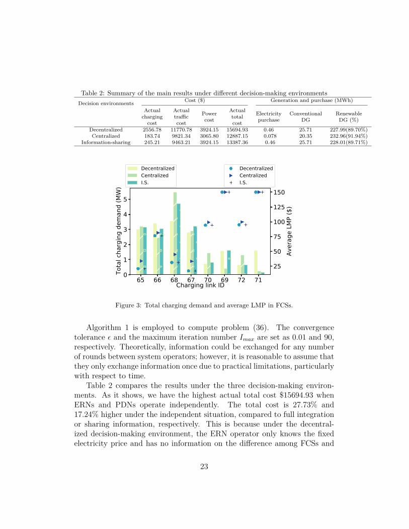
Table 2: Summary of the main results under different decision-making environmentsDecision environments Cost ($) Generation and purchase (MWh)
Actualcharging
cost
Actualtrafficcost
Powercost
Actualtotalcost
Electricitypurchase
ConventionalDG
RenewableDG (%)
Decentralized 2556.78 11770.78 3924.15 15694.93 0.46 25.71 227.99(89.70%)Centralized 183.74 9821.34 3065.80 12887.15 0.078 20.35 232.96(91.94%)
Information-sharing 245.21 9463.21 3924.15 13387.36 0.46 25.71 228.01(89.71%)
65 66 68 67 70 69 72 71Charging link ID
0
1
2
3
4
5
Tota
l cha
rgin
g de
man
d (M
W)
DecentralizedCentralizedI.S.
25
50
75
100
125
150
Aver
age
LMP
($)
DecentralizedCentralizedI.S.
Figure 3: Total charging demand and average LMP in FCSs.
Algorithm 1 is employed to compute problem (36). The convergencetolerance ϵ and the maximum iteration number Imax are set as 0.01 and 90,respectively. Theoretically, information could be exchanged for any numberof rounds between system operators; however, it is reasonable to assume thatthey only exchange information once due to practical limitations, particularlywith respect to time.
Table 2 compares the results under the three decision-making environ-ments. As it shows, we have the highest actual total cost $15694.93 whenERNs and PDNs operate independently. The total cost is 27.73% and17.24% higher under the independent situation, compared to full integrationor sharing information, respectively. This is because under the decentral-ized decision-making environment, the ERN operator only knows the fixedelectricity price and has no information on the difference among FCSs and
23
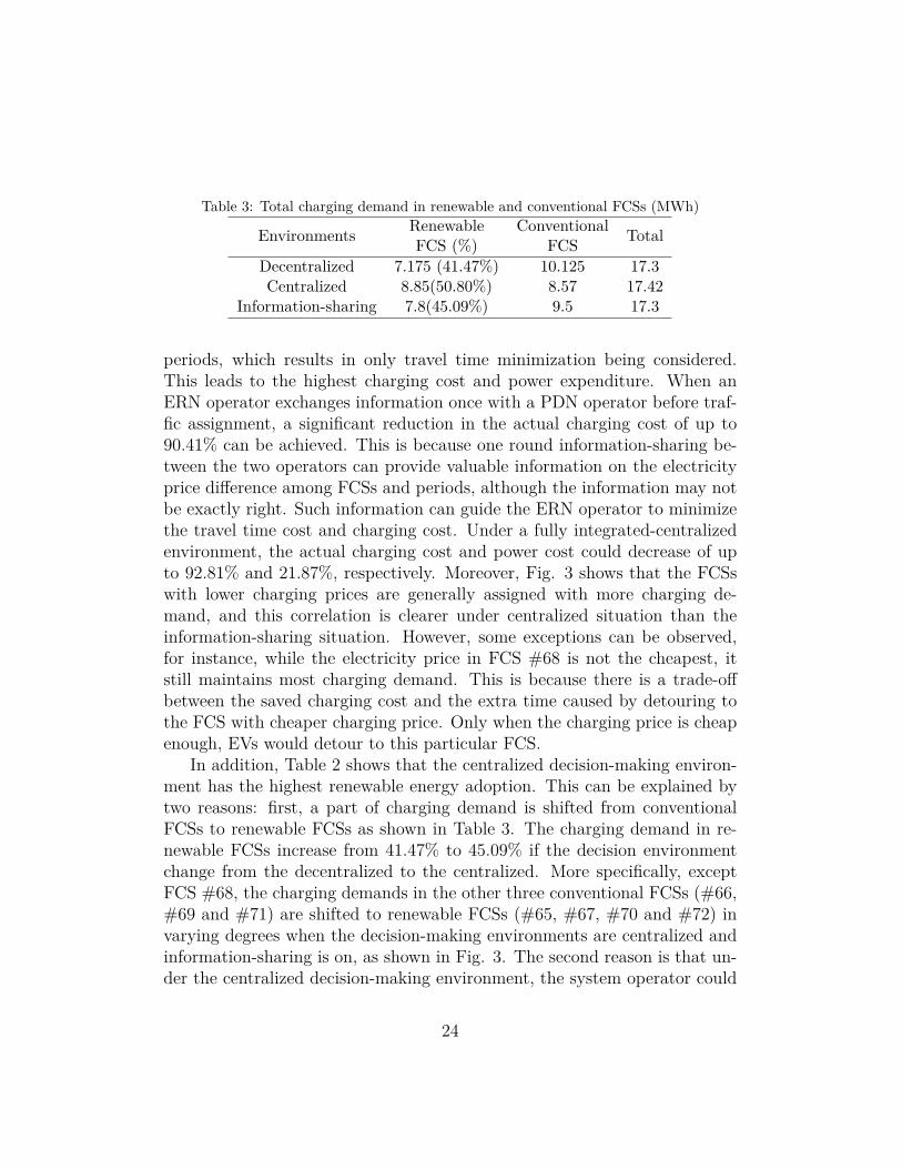
Table 3: Total charging demand in renewable and conventional FCSs (MWh)
Environments RenewableFCS (%)
ConventionalFCS Total
Decentralized 7.175 (41.47%) 10.125 17.3Centralized 8.85(50.80%) 8.57 17.42
Information-sharing 7.8(45.09%) 9.5 17.3
periods, which results in only travel time minimization being considered.This leads to the highest charging cost and power expenditure. When anERN operator exchanges information once with a PDN operator before traf-fic assignment, a significant reduction in the actual charging cost of up to90.41% can be achieved. This is because one round information-sharing be-tween the two operators can provide valuable information on the electricityprice difference among FCSs and periods, although the information may notbe exactly right. Such information can guide the ERN operator to minimizethe travel time cost and charging cost. Under a fully integrated-centralizedenvironment, the actual charging cost and power cost could decrease of upto 92.81% and 21.87%, respectively. Moreover, Fig. 3 shows that the FCSswith lower charging prices are generally assigned with more charging de-mand, and this correlation is clearer under centralized situation than theinformation-sharing situation. However, some exceptions can be observed,for instance, while the electricity price in FCS #68 is not the cheapest, itstill maintains most charging demand. This is because there is a trade-offbetween the saved charging cost and the extra time caused by detouring tothe FCS with cheaper charging price. Only when the charging price is cheapenough, EVs would detour to this particular FCS.
In addition, Table 2 shows that the centralized decision-making environ-ment has the highest renewable energy adoption. This can be explained bytwo reasons: first, a part of charging demand is shifted from conventionalFCSs to renewable FCSs as shown in Table 3. The charging demand in re-newable FCSs increase from 41.47% to 45.09% if the decision environmentchange from the decentralized to the centralized. More specifically, exceptFCS #68, the charging demands in the other three conventional FCSs (#66,#69 and #71) are shifted to renewable FCSs (#65, #67, #70 and #72) invarying degrees when the decision-making environments are centralized andinformation-sharing is on, as shown in Fig. 3. The second reason is that un-der the centralized decision-making environment, the system operator could
24
0 4 8 12 16 20 24 28 32 36time step
6566
6768
6970
7172
Char
ging
link
0.0
0.2
0.4
0.6
0.8
1.0
(a) Decentralized
0 4 8 12 16 20 24 28 32 36time step
6566
6768
6970
7172
Char
ging
link
0.0
0.2
0.4
0.6
0.8
(b) Centralized
0 4 8 12 16 20 24 28 32 36time step
6566
6768
6970
7172
Char
ging
link
0.0
0.2
0.4
0.6
0.8
1.0
(c) Information-sharing
Figure 4: Congestion level of FCS under different decision-making environments.
25
0 5 10 15 20 25 30 35 40time step5.0
5.5
6.0
6.5
7.0
7.5
8.0
8.5
9.0
Tota
l pow
er d
eman
d (M
W) Centralized
DecentralizedI.S.
Figure 5: The time distribution of the total power demand for the studied PDN.
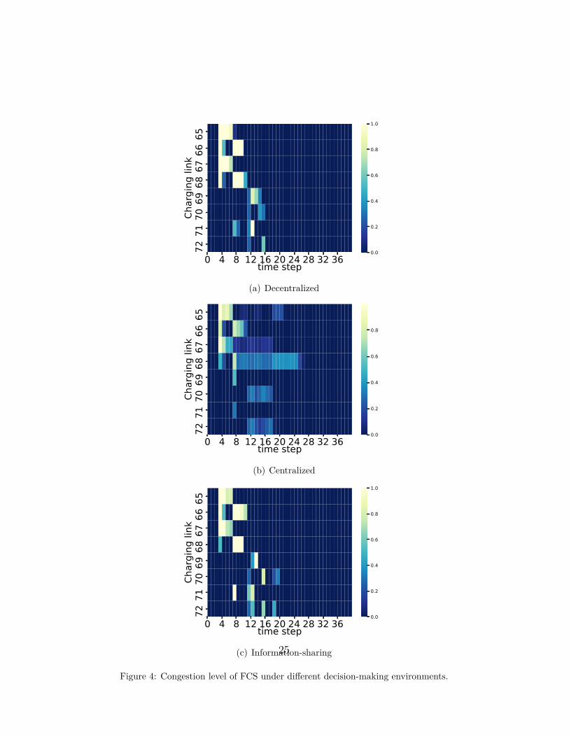
properly assign the charging time and locations of EVs so as to alleviate thecharging congestion in FCSs in peak hours and flatten the the power demandcurve. Note that the generation capacities of renewable DGs are limited ineach period. Consequently, in peak hours, the expensive conventional energycould be replaced by the cheap renewable energy. This can be verified byFigs. 4 and 5. For example, the congestions in charging links 65, 67 and68 are significantly alleviated when two systems operate jointly, as shownin Fig. 4. As a result, the total power demand from the 3rd to the 9thtime step is clipped to from the 13rd to 26th time step, as shown in Fig. 5.In summary, the operator optimizes the charging demand in temporal andspatial aspects to promote the renewable energy integration and, thus, thetotal cost is minimized.
5. Conclusion
This paper proposed a traffic-power system model to investigate the op-erational solution differences when the electric road network (ERN) and thepower distribution network (PDN) operate independently, jointly and withsharing information. The model considered constraints from both ERNs andPDNs, such as road capacity, traffic flow capacity and ramp limit of gener-ators. Within this model, an electric link transmission model (eLTM) was
26
presented to solve the system optimal dynamic traffic assignment problem. Anovel formulation was proposed to accommodate critical physical features ofelectric vehicles (EVs) and fast charging stations (FCSs), such as, EV classeswith different driving ranges, initial state of charge (SoC) of EVs, capacityof FCSs have been considered. Moreover, the charging process of EVs wasexplicitly modeled within the eLTM. The objective of a PDN operator wasto minimize the power cost including power generation cost and purchasefrom the main grid. A numerical example including renewable and conven-tional generators was studied to illustrate the proposed models. The differentdecision-making environments were compared to investigate the correspond-ing operation and social benefits. From the results, we could observe that thecharging cost was the highest under decentralized situation, since the ERNoperator did not know the information on the electricity price differenceamong FCSs and periods. Even limitedly sharing information or operatingjointly between ERNs and PDNs could significantly reduce the charging cost.The increased renewable energy adoption and the flattened power demandcurve assisted in lowering charging cost, power cost and congestion level inFCSs, under a centralized situation. Both electricity price difference amongFCSs and detouring time influenced the charging demand distribution.
This work can be extended in several directions: 1) It is interesting toinvestigate by the proposed eLTM to solve the user equilibrium dynamictraffic assignment (UE-DTA) problem considering critical features of ERNsand FCSs. Although, Refs. [32, 36, 34] claimed that they have solved UE-DTA considering EVs, they oversimplified the critical features of ERNs andFCSs, as shown in Table 1. Therefore, how to solve this problem is stillchallenging. 2) The proposed models can be easily extended to investigatehow the failure spreads between the interdependent traffic-power systems. 3)It is also interesting to investigate how to coordinate the charging demandso as to maximize the renewable energy adoption considering the securityconstraints and the weather conditions.
Appendix A. Data description
A modified electrified road network [28] and power distribution networkis used to illustrated the proposed methods. Figs. A.6 and A.7 show themodified road network and power network. As shown in Fig. A.6, there is onetype charger in each FCS. The green mark on charging links and generatorsrepresents the corresponding FCSs and generators powered by the renewable
27
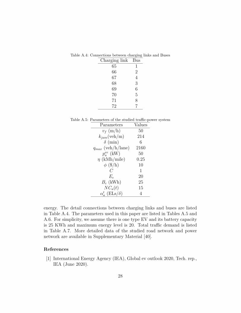
Table A.4: Connections between charging links and BusesCharging link Bus
65 166 267 468 369 670 571 872 7
Table A.5: Parameters of the studied traffic-power systemParameters Valuesvf (m/h) 50
kjam(veh/m) 214δ (min) 6
qmax (veh/h/lane) 2160peva (kW) 50
η (kMh/mile) 0.25ϕ ($/h) 10
C 1Ec 20
Bc (kWh) 25NCa(t) 15
αta (ELs/δ) 4
energy. The detail connections between charging links and buses are listedin Table A.4. The parameters used in this paper are listed in Tables A.5 andA.6. For simplicity, we assume there is one type EV and its battery capacityis 25 KWh and maximum energy level is 20. Total traffic demand is listedin Table A.7. More detailed data of the studied road network and powernetwork are available in Supplementary Material [40].
References
[1] International Energy Agency (IEA), Global ev outlook 2020, Tech. rep.,IEA (June 2020).
28
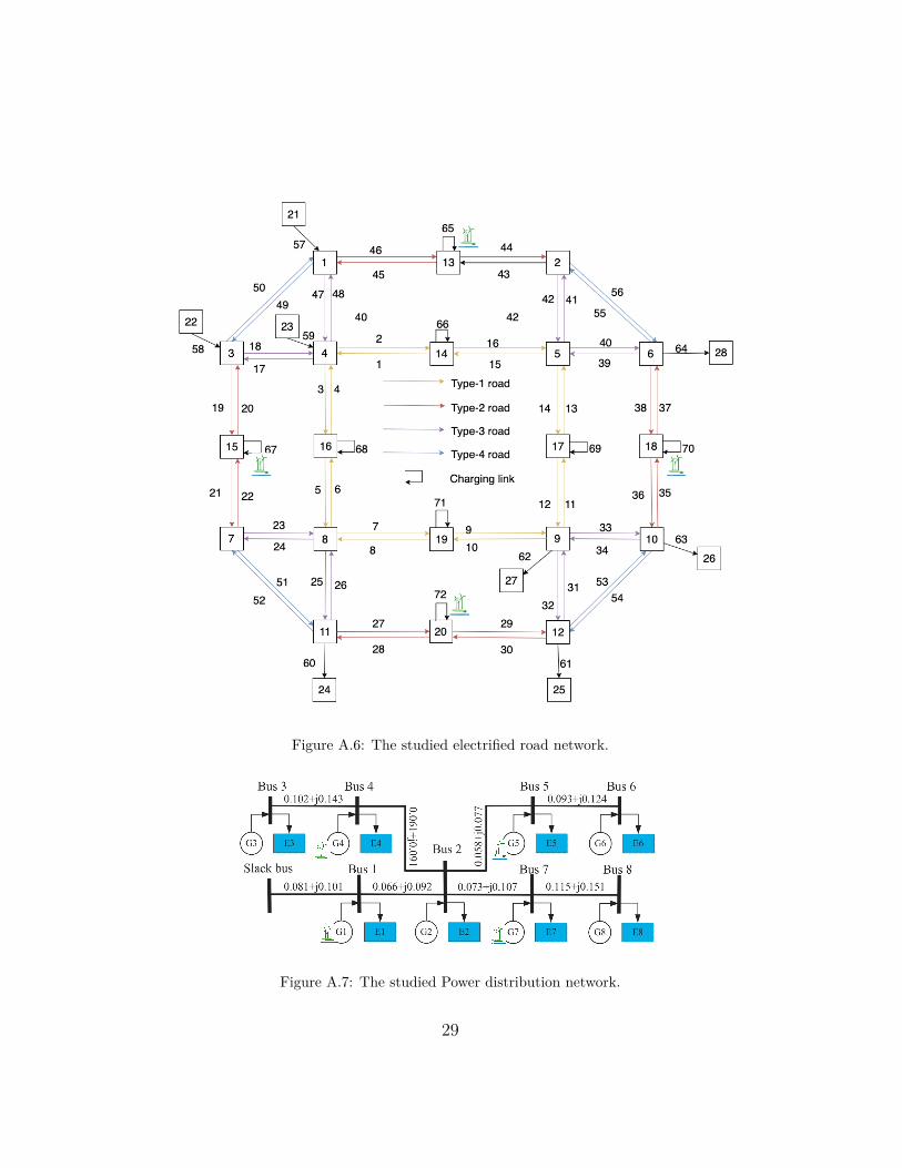
Figure A.6: The studied electrified road network.
Figure A.7: The studied Power distribution network.
29
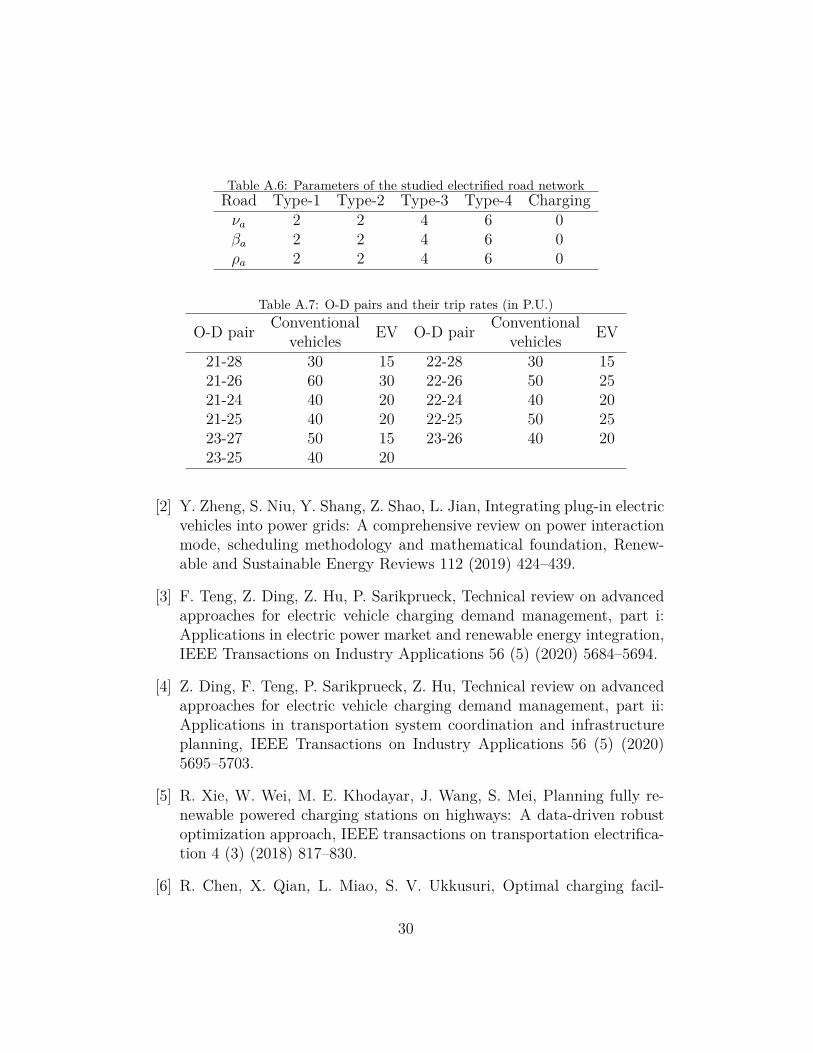
Table A.6: Parameters of the studied electrified road networkRoad Type-1 Type-2 Type-3 Type-4 Chargingνa 2 2 4 6 0βa 2 2 4 6 0ρa 2 2 4 6 0
Table A.7: O-D pairs and their trip rates (in P.U.)
O-D pair Conventionalvehicles EV O-D pair Conventional
vehicles EV
21-28 30 15 22-28 30 1521-26 60 30 22-26 50 2521-24 40 20 22-24 40 2021-25 40 20 22-25 50 2523-27 50 15 23-26 40 2023-25 40 20
[2] Y. Zheng, S. Niu, Y. Shang, Z. Shao, L. Jian, Integrating plug-in electricvehicles into power grids: A comprehensive review on power interactionmode, scheduling methodology and mathematical foundation, Renew-able and Sustainable Energy Reviews 112 (2019) 424–439.
[3] F. Teng, Z. Ding, Z. Hu, P. Sarikprueck, Technical review on advancedapproaches for electric vehicle charging demand management, part i:Applications in electric power market and renewable energy integration,IEEE Transactions on Industry Applications 56 (5) (2020) 5684–5694.
[4] Z. Ding, F. Teng, P. Sarikprueck, Z. Hu, Technical review on advancedapproaches for electric vehicle charging demand management, part ii:Applications in transportation system coordination and infrastructureplanning, IEEE Transactions on Industry Applications 56 (5) (2020)5695–5703.
[5] R. Xie, W. Wei, M. E. Khodayar, J. Wang, S. Mei, Planning fully re-newable powered charging stations on highways: A data-driven robustoptimization approach, IEEE transactions on transportation electrifica-tion 4 (3) (2018) 817–830.
[6] R. Chen, X. Qian, L. Miao, S. V. Ukkusuri, Optimal charging facil-
30
ity location and capacity for electric vehicles considering route choiceand charging time equilibrium, Computers & Operations Research 113(2020) 104776.
[7] R. Vosooghi, J. Puchinger, J. Bischoff, M. Jankovic, A. Vouillon, Sharedautonomous electric vehicle service performance: Assessing the impactof charging infrastructure, Transportation Research Part D: Transportand Environment 81 (2020) 102283.
[8] T. Qian, C. Shao, X. Wang, M. Shahidehpour, Deep reinforcement learn-ing for ev charging navigation by coordinating smart grid and intelligenttransportation system, IEEE Transactions on Smart Grid 11 (2) (2019)1714–1723.
[9] M. M. Nejad, L. Mashayekhy, D. Grosu, R. B. Chinnam, Optimal rout-ing for plug-in hybrid electric vehicles, Transportation Science 51 (4)(2017) 1304–1325.
[10] G. Hiermann, R. F. Hartl, J. Puchinger, T. Vidal, Routing a mix ofconventional, plug-in hybrid, and electric vehicles, European Journal ofOperational Research 272 (1) (2019) 235–248.
[11] L. Bedogni, L. Bononi, M. Di Felice, A. D’Elia, R. Mock, F. Morandi,S. Rondelli, T. S. Cinotti, F. Vergari, An integrated simulation frame-work to model electric vehicle operations and services, IEEE Transac-tions on vehicular Technology 65 (8) (2016) 5900–5917.
[12] B. Wang, P. Dehghanian, S. Wang, M. Mitolo, Electrical safety consid-erations in large-scale electric vehicle charging stations, IEEE Transac-tions on Industry Applications 55 (6) (2019) 6603–6612.
[13] A.-M. Hariri, M. A. Hejazi, H. Hashemi-Dezaki, Investigation of impactsof plug-in hybrid electric vehicles’ stochastic characteristics modelingon smart grid reliability under different charging scenarios, Journal ofCleaner Production 287 (2021) 125500.
[14] D. Tang, P. Wang, Nodal impact assessment and alleviation of movingelectric vehicle loads: From traffic flow to power flow, IEEE Transactionson Power Systems 31 (6) (2016) 4231–4242.
31
[15] V. H. Fan, Z. Dong, K. Meng, Integrated distribution expansion plan-ning considering stochastic renewable energy resources and electric ve-hicles, Applied Energy 278 (2020) 115720.
[16] L. Luo, W. Gu, S. Zhou, H. Huang, S. Gao, J. Han, Z. Wu, X. Dou,Optimal planning of electric vehicle charging stations comprising multi-types of charging facilities, Applied energy 226 (2018) 1087–1099.
[17] B. Zhou, G. Chen, Q. Song, Z. Y. Dong, Robust chance-constrainedprogramming approach for the planning of fast-charging stations in elec-trified transportation networks, Applied Energy 262 (2020) 114480.
[18] R. Gupta, A. Pena-Bello, K. N. Streicher, C. Roduner, D. Thöni, M. K.Patel, D. Parra, Spatial analysis of distribution grid capacity and coststo enable massive deployment of pv, electric mobility and electric heat-ing, Applied Energy 287 (2021) 116504.
[19] R. Tu, Y. J. Gai, B. Farooq, D. Posen, M. Hatzopoulou, Electric vehiclecharging optimization to minimize marginal greenhouse gas emissionsfrom power generation, Applied Energy 277 (2020) 115517.
[20] M. R. Islam, H. Lu, M. J. Hossain, L. Li, Optimal coordination of elec-tric vehicles and distributed generators for voltage unbalance and neu-tral current compensation, IEEE Transactions on Industry Applications57 (1) (2020) 1069–1080.
[21] A. Zahedmanesh, K. M. Muttaqi, D. Sutanto, Coordinated chargingcontrol of electric vehicles while improving power quality in power gridsusing a hierarchical decision-making approach, IEEE Transactions onVehicular Technology 69 (11) (2020) 12585–12596.
[22] Z. Liu, Q. Wu, K. Ma, M. Shahidehpour, Y. Xue, S. Huang, Two-stage optimal scheduling of electric vehicle charging based on transactivecontrol, IEEE Transactions on Smart Grid 10 (3) (2019) 2948–2958.
[23] S. Xie, Z. Hu, J. Wang, Two-stage robust optimization for expansionplanning of active distribution systems coupled with urban transporta-tion networks, Applied Energy 261 (2020) 114412.
32
[24] T. Yang, Q. Guo, L. Xu, H. Sun, Dynamic pricing for integrated energy-traffic systems from a cyber-physical-human perspective, Renewable andSustainable Energy Reviews 136 (2021) 110419.
[25] H. Wang, Y.-P. Fang, E. Zio, Risk assessment of an electrical powersystem considering the influence of traffic congestion on a hypotheticalscenario of electrified transportation system in new york state, IEEETransactions on Intelligent Transportation Systems 22 (1) (2021) 142–155.
[26] M. Shin, D.-H. Choi, J. Kim, Cooperative management for pv/ess-enabled electric vehicle charging stations: A multiagent deep reinforce-ment learning approach, IEEE Transactions on Industrial Informatics16 (5) (2019) 3493–3503.
[27] H. Zhang, Z. Hu, Y. Song, Power and transport nexus: Routing electricvehicles to promote renewable power integration, IEEE Transactions onSmart Grid 11 (4) (2020) 3291–3301.
[28] W. Wei, L. Wu, J. Wang, S. Mei, Network equilibrium of coupled trans-portation and power distribution systems, IEEE Transactions on SmartGrid 9 (6) (2018) 6764–6779.
[29] X. Wang, M. Shahidehpour, C. Jiang, Z. Li, Coordinated planning strat-egy for electric vehicle charging stations and coupled traffic-electric net-works, IEEE Transactions on Power Systems 34 (1) (2018) 268–279.
[30] L. Geng, Z. Lu, L. He, J. Zhang, X. Li, X. Guo, Smart charging manage-ment system for electric vehicles in coupled transportation and powerdistribution systems, Energy 189 (2019) 116275.
[31] S. Xie, Z. Hu, J. Wang, Y. Chen, The optimal planning of smart multi-energy systems incorporating transportation, natural gas and active dis-tribution networks, Applied Energy 269 (2020) 115006.
[32] Z. Zhou, X. Zhang, Q. Guo, H. Sun, Analyzing power and dynamictraffic flows in coupled power and transportation networks, Renewableand Sustainable Energy Reviews 135 (2021) 110083.
[33] F. Rossi, R. Iglesias, M. Alizadeh, M. Pavone, On the interaction be-tween autonomous mobility-on-demand systems and the power network:
33

Models and coordination algorithms, IEEE Transactions on Control ofNetwork Systems 7 (1) (2019) 384–397.
[34] S. Lv, Z. Wei, G. Sun, S. Chen, H. Zang, Optimal power and semi-dynamic traffic flow in urban electrified transportation networks, IEEETransactions on Smart Grid 11 (3) (2019) 1854–1865.
[35] S. Lv, Z. Wei, S. Chen, G. Sun, D. Wang, Integrated demand responsefor congestion alleviation in coupled power and transportation networks,Applied Energy 283 (2021) 116206.
[36] G. Sun, G. Li, S. Xia, M. Shahidehpour, X. Lu, K. W. Chan, Aladin-based coordinated operation of power distribution and traffic networkswith electric vehicles, IEEE Transactions on Industry Applications56 (5) (2020) 5944–5954.
[37] I. Yperman, The link transmission model for dynamic network loading.
[38] J. Long, W. Y. Szeto, Link-based system optimum dynamic traffic as-signment problems in general networks, Operations Research 67 (1)(2019) 167–182.
[39] F. He, Y. Yin, S. Lawphongpanich, Network equilibrium models withbattery electric vehicles, Transportation Research Part B: Methodolog-ical 67 (2014) 306–319.
[40] H. Wang, A. F. Abdin, Y.-P. Fang, E. Zio, Supplementary material,https://github.com/lucky105/Coordinating-dynamic-traffic-power-systems-under-decentralized-centralized-and-formation-sharing,accessed April. 2, 2021 (2021).
34