coordination control of distributed spacecraft system...6 coordination control of distributed...

6

Coordination Control of Distributed Spacecraft System

Min Hu1, Guoqiang Zeng2 and Hong Yao1 1Academy of Equipment, Beijing,

2College of Aerospace and Material Engineering, National University of Defense Technology, Changsha,

China

1. Introduction

Spacecraft formation flying has received significant attention over the past decade, it has been a topic of interest because of its unique technical advantages and good application features. Several small, unconnected satellites operating in a coordinated way may achieve a better performance than a monolithic satellite, and possess advantages such as increased instrument resolution, reduced cost, reconfigurability, and overall system robustness, which can in turn enhance the scientific return (Zhang et al., 2008).Several ambitious distributed spacecraft missions are currently being put in operation or planned. The PRISMA satellite, which is an on-orbit technology demonstrator for autonomous formation flying and rendezvous, was launched on 15 June 2010 (Ardaens et al., 2011). The TanDEM-X satellite was launched on 21 June 2010 and orbited in close formation with the TerraSAR–X satellite on 15 October 2010. The twin satellites began a routine acquisition of the digital elevation model with flexible baselines on 12 December 2010 (Kahle et al., 2011). The F6 program of the Defense Advanced Research Projects Agency, the Terrestrial Planet Finder of the National Aeronautics and Space Administration, and the Darwin mission of the European Space Agency will all utilize the technology of formation flying.

The modelling of relative motion of distributed spacecraft has been extensively investigated in the past. The Hill-Clohessy-Wiltshire (HCW) equations are widely used. The equations describe the relative motion of two close formation flying satellites in near circular orbits about a spherical Earth, and no disturbances are included in the Hill equations. Using orbital elements to parameterize the relative motion is another important way (D’Amico & Montenbruck, 2006; Ardaens & D’Amico, 2009), which is extremely efficient and was successfully demonstrated during the swap of the GRACE satellites (Montenbruck et al., 2006). By a proper design of the relative orbit elements, a minimum distances in the cross-track plane is guaranteed and the collision hazard is minimized.

In recent years, a significant amount of work has been focused on formation relative orbit estimation. Liu considered the relative navigation for formation flying using an unscented Kalman filter (UKF) and showed that the error of the relative position and velocity estimation can be estimated in the centimeter and millimeter per second scales, respectively (Liu et al., 2008). The original Kalman filter is widely used in relative navigation; however,

www.intechopen.com

Advances in Spacecraft Systems and Orbit Determination

124

its inherent linearization process typically introduces significant biases in the estimation results. A particle filter (PF) achieves a recursive Bayesian estimation via a non-parametric Monte Carlo method and shows significant advantages in the nonlinear estimation problem (Rigatos, 2009). A way of generating the importance density function of a PF is essential to improve its performance. EKF and UKF are effective in generating the importance density function.Therefore, because of the strong non-linearity of the dynamics of satellites formation flying; the extended PF (EPF) is adopted to improve the precision of the relative orbit estimation for autonomous formation flying. Moreover, the nonlinear least squares method is applied to determine the relative orbit for the ground-in-the-loop control mode, which is more accurate and suit for the short-arc observation data of the ground station.

An accurate relative orbit control is also very important for the practical implementation of distributed spacecraft. A number of effective controllers are presented in recent literature, such as the linear quadratic regulator, the sliding mode control, and relative orbital elements. Scharf divided the formation flying control problem into five architectures: Leader/Follower, Multiple-Input Multiple-output, Virtual Structure, Cyclic, and Behavioral. We adopt the Leader/Follower approach for practical implementation (Scharf et al., 2004).

It is now known that finite-time stabilization of dynamical system usually demonstrate some nice features such as finite-time convergence to the equilibrium, high-precision performance, faster response as well as better disturbance rejection properties (Ding & Li, 2011). A number of effective methods to achieve the FTC are presented in recent literature (Wu et al., 2011), such as the time-optimal control, TSM control, adaptive control, homogeneous system approach and finite time stability approach. TSM control has been widely used in many applications. By designing a nonlinear switching manifold, the states reach the equilibrium in finite time and exhibit insensitive properties, such as robustness to parameter perturbations and external disturbances (Hu et al., 2008). Man proposed a robust control scheme for rigid robotic manipulators using the TSM technique (Man et al., 1994). However, the controller has a singularity problem. Feng presented a global non-singular TSM controller for a second-order nonlinear dynamic systems (Feng et al., 2002). On the one hand, TSM controllers converge to the equilibrium quickly once in the neighbourhood of the equilibrium, however, when the states are far away from the equilibrium, the system states converge slowly. On the other hand, the linear-hyperplane-based sliding mode controllers converge to the equilibrium quickly when the states are far away from the equilibrium, but they only guarantee asymptotic stability and convergence. All these controllers can not achieve global fast convergence performance in finite time. Therefore, the current study concentrates on the FTC technique to deal with this problem. Currently, the FTC approach has been applied in many fields, such as spacecraft attitude tracking control, consensus for multi-agent systems, robotic manipulators control and missile guidance law design. We will adopt the FTC approach for formation maintenance.

With an increasing number of projects in operation, a practical formation control has also become an area of concern. Relative orbital elements were demonstrated during the GRACE, PRISMA, and TanDEM-X missions. Therefore, the current study will concentrate on formation reconfiguration based on relative orbital elements. Ardaens and D'Amico proposed a dual-impulse method for the in-plane relative control and a single-impulse control for the cross-track motion (Ardaens & D’Amico, 2009); when the control period increases, the dual-impulse maneuver causes an additional along-track drift. Hence, the use

www.intechopen.com


125

of a dual-impulse maneuver for an extended control period of formation keeping may be restricted. The formation reconfiguration control is divided into fuel-optimal triple-impulse in-plane motion control and single-impulse cross-track motion control.

Safe trajectory planning methods are often employed in collision avoidance maneuver. By

considering the minimum distances among the satellites as the constraints, safe trajectories

can be generated using various planning algorithms, and collision avoidance can be realized

by controlling the satellites along the planned trajectory. Tillerson and Richards introduced

fuel-optimal trajectories for spacecraft using mixed-integer linear programming, which

includes various avoidance constraints (Tillerson et al., 2002; Richards et al., 2002). The

artificial potential function method for formation flying satellites has also received

considerable attention in recent years (Nag et al., 2010; Bevilacqua et al., 2011). By

constructing artificial fields, the goal position provides the attractive forces, whereas the

collision avoidance constraints provide the repulsive forces, thereby enabling formation

flying satellites to move into their target positions without colliding. Mueller used a robust

linear programming technique for the collision avoidance manoeuvre of the PRISMA

mission, enabling the satellites to rapidly exit the avoidance region through the application

of a single impulse at a specified time (Mueller, 2009; Muelleret et al., 2010). Therefore, the

linear programming algorithms are used for the collision avoidance manoeuvre of

proximity operations.

The topics concerning simulation or experiment testbeds which focus on the verification of

the new technologies of distributed spacecraft have been studied by many researchers in

recent years. J. Leitner firstly developed a closed-loop hardware-in-the-loop simulation

environment for GPS based formation flying (Leitner, 2001). The SPHERES testbed provided

a verification environment for formation flying, rendezvous, docking and autonomy

algorithms (Mark, 2002). Wang developed a real-time simulation framework for

development and verification for formation flying satellites, which provides access of real

sensor system via serial interface (Wang &Zhang, 2005). D’Amico presented an offline and

hardware -in-the-loop validation of the GPS-based real-time navigation system for the

PRISMA formation flying mission (D’Amico et al., 2008). D’Amico developed the TanDEM-

X Autonomous Formation Flying (TAFF) system which is to support the design,

implementation, testing and validation of real-time embedded GPS-based GNC system

(D’Amico et al., 2009).

The organization of this chapter is as follows: In Section 2, the relative orbit dynamics are

introduced, and the general formation description parameters are presented. In Section 3,

the relative orbit estimation based on extended particle-filter and nonlinear least squares are

presented, respectively. The different coordination control methods are proposed in Section

4. Section 5 presents the processor-in-the-loop distributed simulation system. Section 6

summarizes our conclusions.

2. Preliminaries

With respect to a near-circular reference orbit, and assuming the satellites are taken

sufficiently close to each other, the relative motion given by several Keplerian elements

differing can be treated to first order.

www.intechopen.com


126

2.1 Coordinate systems

The relative motion dynamics has been discussed in many papers. We consider two neighbour satellites flying in Earth orbit. The inertial reference frame used is the J2000 frame. The origin of the coordinate system is the centre of the Earth; the XI axis points toward the mean equinox of J2000.0, the ZI axis points toward the mean north celestial pole of J2000.0, and the YI axis completes the right-handed system. The relative reference frame used is the Hill frame. The origin of the coordinate system is placed at the centre of mass of the master satellite; the x axis is aligned in the radial direction, the z axis is aligned with the angular momentum vector and the y axis completes the right-handed system (Fig. 1).

IX

IY

IZ

i

f

x

y

z

Fig. 1. J2000 inertial frame and Hill frame.

2.2 Relative orbit dynamics

2.2.1 Dynamics equations

With respect to the circular reference orbit, the relative motion can be described as the

following equations:

2

2

2 3 0

2 0

0

x ny n x

y nx

z n z

(1)

where [ ]x y z x y z is the relative position and velocity in Hill’s frame, n is the mean

orbit rate.

The relative dynamics for the circular orbits can be expressed in a linear time-invariant (LTI) system in state-space.

( ) ( ) ( )

( ) ( )

x x u

y x

t A t B t

t C t (2)

www.intechopen.com


127

where x is the state vector in Hill’s frame, u is the applied acceleration in Hill’s frame and

y is the output which is equal to the state vector(C is identity).

For a circular reference orbit, the A and B are independent of time:

2

2

0 0 0 1 0 0 0 0 0

0 0 0 0 1 0 0 0 0

0 0 0 0 0 1 0 0 0

3 0 0 0 2 0 1 0 0

0 0 0 2 0 0 0 1 0

0 0 10 0 0 0 0

A Bn n

n

n

(3)

2.2.2 Kinematics equations

The Keplerian orbital elements are a , e , i , , , and u , which correspond to the semi-

major axis, eccentricity, inclination, right ascension of the ascending node, argument of

perigee, and mean argument of latitude ( u M , where M is the mean anomaly, and

can be obtained from the true anomaly f ), respectively. Spacecraft-1 is the master satellite,

and Spacecraft-2 is the deputy satellite. For near-circular satellite orbits, the relative

eccentricity vector can be defined as follows:

2 1

2 12 1

cos cos cos

sin sinsin

x

y

ee e e

e

e (4)

where e represents the amplitude of e and defines the initial phase angle of the in-

plane motion.

The inclination vector i can be defined using the law of sines and cosines for the spherical

triangle:

1

cos

sinsin

x

y

i ii

i i

i (5)

where 2 1 i i i , 2 1- , i represents the amplitude of i , and defines the

initial phase angle of the cross-track plane motion.

2.3 General formation configuration description parameters

For a near-circular reference orbit, the relative motion of the formation flying satellites can

be described by the following equations (Hu et al., 2010):

cos( )

2 sin( )

sin( )

x a p u

y p u l

z s u

(6)

www.intechopen.com


128

where , , , ,p s l are the five general formation configuration description parameters;

p a e represents the semi-minor axis of the relative in-plane ellipse; s a i denotes the

cross-track amplitude; defines the relative initial phase angle between the in-plane

and cross-track plane motions; and is the initial phase angle of the in-plane motion.

2 1 u u u , 0

3( cos ) ( )

2 l a u i u u a , 0u is the initial mean argument of latitude of

the deputy satellite, and l represents the along-track offset of the centre of the in-plane

motion. An example trajectory is shown in Fig. 2.

x

y

p

l

deputy deputy

x

z

p

s

θ φ

Fig. 2. Example of a relative motion in a near-circular reference orbit.

2.4 Passively safe formation configuration

The distance in the cross-track plane can be expressed as

2 2 r x z (7)

By substituting equation (6) into equation (7), we obtain r :

2 2 2 2

2 2 2 2 cos2( ) cos2( )cos ( ) sin ( )

2

p s p u s ur p u s u

(8)

where

2 2 2 2 2 2

4 4 2 2 4 4 2 2

[ cos2( ) cos2( )] [ sin2( ) sin2( )]

2 cos2( ) 2 cos2

p u s u p u s u

p s p s p s p s

(9)

so that

2 2 4 4 2 2cos2( ) cos2( ) 2 cos2 p u s u p s p s (10)

Minimum distance minr in the cross-track plane is

2 2 4 4 2 2

min

2 cos2

2

p s p s p sr

(11)

www.intechopen.com


129

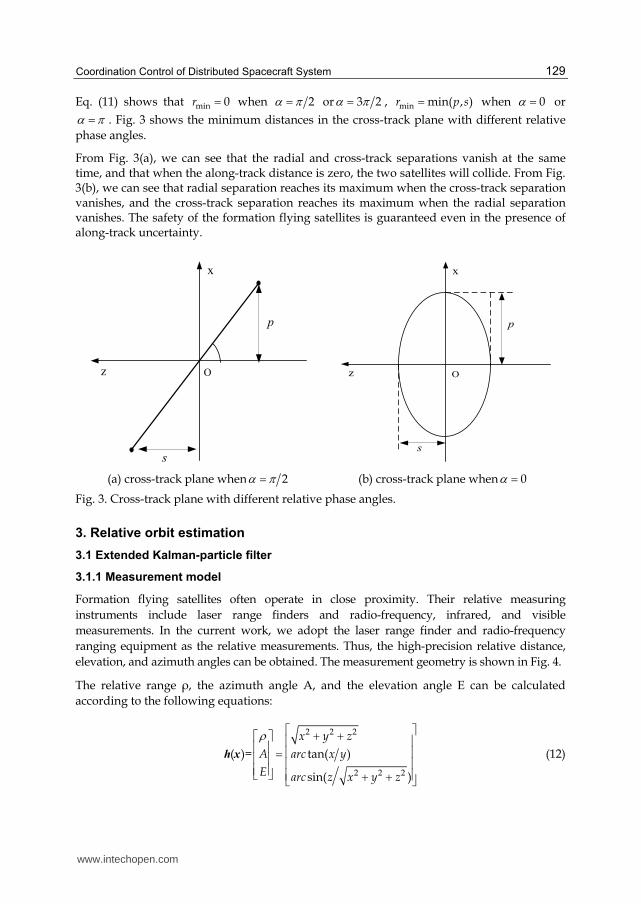
Eq. (11) shows that min 0r when 2 or 3 2 , min min( , )r p s when 0 or

. Fig. 3 shows the minimum distances in the cross-track plane with different relative

phase angles.

From Fig. 3(a), we can see that the radial and cross-track separations vanish at the same time, and that when the along-track distance is zero, the two satellites will collide. From Fig. 3(b), we can see that radial separation reaches its maximum when the cross-track separation vanishes, and the cross-track separation reaches its maximum when the radial separation vanishes. The safety of the formation flying satellites is guaranteed even in the presence of along-track uncertainty.

x

z O

s

p

x

z O

s

p

(a) cross-track plane when 2 (b) cross-track plane when 0

Fig. 3. Cross-track plane with different relative phase angles.

3. Relative orbit estimation

3.1 Extended Kalman-particle filter

3.1.1 Measurement model

Formation flying satellites often operate in close proximity. Their relative measuring

instruments include laser range finders and radio-frequency, infrared, and visible

measurements. In the current work, we adopt the laser range finder and radio-frequency

ranging equipment as the relative measurements. Thus, the high-precision relative distance,

elevation, and azimuth angles can be obtained. The measurement geometry is shown in Fig. 4.

The relative range ρ, the azimuth angle A, and the elevation angle E can be calculated

according to the following equations:

2 2 2

2 2 2

( )= tan( )

sin( )

x y z

A arc x y

E arc z x y z

h x (12)

www.intechopen.com


130

where ( )h x is the measurement matrix, and x, y, and z are the coordinates of the deputy

satellite in the body-fixed frame of the master satellite. As we know, the transformation

matrix between the body-fixed frame and the Hill frame is a function of the attitude of the

master satellite. In this paper, the attitude determination problem was not considered.

Therefore, the relative measurements are defined with respect to the Hill frame.

x

y

z

'h

h

o A

E

Fig. 4. Relative measurement geometry.

The state and measurement equations can be established as follows:

1( , )

( , )

k k k k

k k k k

f t

h t

X X W

Y X V (13)

where kX is the relative state vector in the Hill frame at time kt ; kY is the relative

measurements at time kt , which can be obtained using Eq. (12); kW is the zero mean value

white Gaussian process noise with the covariance kQ ; and kV is the zero mean value white

Gaussian observation noise with the covariance kR .

Five typical measurement errors, namely, the relative range and angle measurement error, the absolute position and velocity measurement error, and the attitude determination error, are considered.

3.1.2 EPF algorithm

The Kalman filter is the most common method of relative navigation. However, the PF shows better performance in a nonlinear relative state and measurement equations. The principle of PF is to implement the recursive Bayesian filter using Monte Carlo simulations, in which the choice of the importance density function is very important. We employ EKF to realize the importance sampling, which not only makes full use of the latest measurement information, but also avoids the particle exhaustion problem. The particle weights, which are closely associated with the observation, increase, whereas the other particle weights decrease.

The EPF algorithm is summarized as follows: the variable 0( )p x is the prior probability

density; 1ˆ k kx and ˆk kx are the predicted and updated estimates of the states at time kt ,

respectively; 1k kP and k kP are their error covariance matrices, respectively; , 1k k is the

www.intechopen.com


131

state transition matrix, kK represents the Kalman gain matrix; and ikw represents the

importance weight. The Jacobian matrix kH is defined as follows:

1ˆ

( , )

k k

k kk

k x

h tH

X

X (14)

We initialize the particles using:

0 0 0( ), 1 1,2, , i ix p x w N i N

Importance sampling:

a. The particles are updated using the following equations:

1 , 1 1 1 1

1 , 1 1 1 , 1 1

11 1

1 1

1

ˆ

[ ]

ˆˆ ˆ [ ]

[ ]

k k k k k k k

Tk k k k k k k k k

T Tk k k k k k k k k

k k k k k k k k k

k k k k k k

x x Q

P P Q

K P H H P H R

x x K Y H x

P I K H P

0: 1 1:ˆ ( | , ) ( , ) 1,2, , i i i i

k k k k k kx q x x y N x P i N

b. The importance weights are calculated using the following equations:

1 1 1 1:

1

ˆ ˆ ˆ ˆ( | ) ( | ) / ( | , )

/

i i i i i i ik k k k k k k k k

Ni i ik k k

i

w w p y x p x x q x x y

w w w1,2, , i N

Re-sampling is conducted using

/ /ˆ ˆ, ,1i i i

k k k k k kx w x N 1,2, , i N

Thus, the state update is expressed as follows:

1

ˆ 1,2, ,

N

i ik k k

i

x w x i N

3.2 Nonlinear least squares method

The nonlinear state equation and observation equation are as follows (Hu et al., 2010):

0 ,l lf tX X (15)

, l l l ltY G X V (16)

www.intechopen.com


132

where lX is the state vector at the time lt , which includes the J2 perturbations. lY is the

observation vector at the time lt . lV is the observation noise with normal Gauss

distribution.

Equation (16) can expanded at the approximation point *0X by using the Taylor series

equation, the following equations can be derived by keeping the linear items:

* * *0 0 0 0, , l l l lt tY G X A X X X V (17)

where

*

0 0

*0

0

,

l ll

l

t

X X

Y XA X

X X (18)

,

l ll

l l

tt

G XYH

X X (19)

0

00 0

,,

ll f t

t tXX

X X (20)

Let *0 , l l lty Y G X and *

0 0 0 x X X , we get the linear equation as follows:

0 0, l lt t ty H x V (21)

where lV is the residual error, ( )tH is the Jacobian matrix. The transition matrix 0,t t

can be calculated as follows:

*

0 0, ,

t t t t t

ft

X

F

FX

Therefore, the nonlinear model turns out to be the following form:

,0 0

l l

l l l l

X X

Y A X V

(22)

By using the least square method, the estimation value of epoch time can be derived by iteration:

1

0/1 1

ˆ

k k

T Tk l l l l

l l

x A A A y (23)

The optimal estimation should be calculated iteratively, and usually can converge by 3-5 steps.

www.intechopen.com


133

3.3 Numerical simulations and results analysis

A numerical simulation is conducted to verify the effectiveness of the presented EPF

algorithm. The simulation conditions are as follows: the mean orbital elements of the master

and deputy satellites are as shown in Table 1, and Fig. 5 shows the three-dimensional

formation configuration. The formation configuration parameters are p = 400 m, s = 350 m, = 0°, = 90°, l = 0 m. The absolute position and velocity measurement precision are 10 m

and 0.1 m/s, respectively; and the relative range and angle measurement precision are 0.1 m

and 0.01°, respectively. The sampling interval is 1 s. Perturbations of Earth oblateness,

atmospheric drag, solar radiation pressure, perturbation of the third-body of the sun and

moon, and perturbation of the earth body tide are considered in the dynamics simulation.

The fourth-order Runge–Kuta algorithm is employed for the numerical integration.

a (m) e i (deg) (deg) (deg) M (deg)

master 6892937.0 0.001170 97.443823 100.0 90.0 0.0

deputy 6892937.0 0.001112 97.443823 99.997066 89.999620 0.0

Table 1. Mean orbital elements of the master and deputy satellites.

The absolute orbit of the master and deputy satellites can be generated using the Satellite Tool Kit based on the initial elements given in Table 1. The observation values can be simulated by the absolute orbit information and the measurement covariance using the Gaussian distribution random number series. The measurement sampling period is 1 s, and the simulation time is 3000 s.

-600

-400

-200

0

200

400

600

800

-200

0

200

-400

-200

0

200

Along-track/m

Cross-track/m

Radia

l/m

Fig. 5. Three-dimensional formation configuration.

The relative position and velocity estimation errors are shown in Figs. 6 and 7, respectively. The estimation curves are globally convergent, and the EPF algorithm achieved much faster convergence rate in the relative orbit estimation. The relative position estimation errors converge to 210-2 m within 500 s, and that of the relative velocity estimation are within 110-4 m/s.

www.intechopen.com


134

500 1000 1500 2000 2500 3000-0.03

-0.02

-0.01

0

0.01

0.02

0.03

Time(s)

Rela

tive p

ositi

on e

rror(

m)

x

y

z

Fig. 6. Relative position estimation errors.

500 1000 1500 2000 2500 3000-1

0

1x 10

-4

Time(s)

Rela

tive v

elo

city

err

or(

m/s

)

vx

vy

vz

Fig. 7. Relative velocity estimation errors.

4. Relative orbit control

4.1 Coordinated control scheme

We consider an operational scenario with two formation flying satellites, and the deputy

satellite performs the relative orbit correction maneuvers. Fig. 8 shows the schematic

diagram of the formation flying guidance, navigation, and control (GNC) system.

The deputy satellite obtains the relative measurements and performs the relative orbit

estimation to obtain the high-precision relative position and velocity. The formation control

software generates control commands according to the current states and mission goals.

Thrusters are used to control the geometry and phase angle of the formation, and the yaw

angle maneuver commands are used to control the along-track drift. The ground station can

monitor the formation flying system in autonomous mode and generate formation control

commands in the ground-in-the-loop mode.

www.intechopen.com


135

Fig. 8. Schematic diagram of the formation flying GNC system.

4.2 Finite time control for formation maintenance

4.2.1 Control objective

The finite-time control for distributed spacecraft is to design the controller mu which

guarantees that the trajectory tracking errors of the deputy satellite with respect to the

master satellite converge to zero in finite time.

The trajectory tracking errors are defined as

, d de e (24)

where d , and 3d R are the desired relative position and velocity vectors, respectively.

4.2.2 Finite-time controller

In this section, a robust sliding mode controller is proposed to improve the transient performance and to guarantee the finite-time stability and convergence. The formation

www.intechopen.com


136

flying satellites are close to each other, thus, the disturbances acting on the satellites will be

almost the same, and the total relative disturbances D can generally be treated as bounded

forces. Suppose that i iD F , 1,2,3i , where iF is a positive constant.

We propose the following controller

1

( ) ( , , ) sgn( ) n nC N

m du r e e e k S (25)

where , 0 , 0ik , 1,2,3i , 0 1 . S is given by

sgn( ) S e e + e e (26)

Theorem 1. For the formation flying system, the controller (25) can achieve the control objective of trajectory tracking presented in Section 4.2.1.

Proof: Step 1: The system will reach the sliding mode 0S in finite time.

Consider Lyapunov function

1

2 TV S S (27)

Obtaining the time-derivative of V

1

1

( )

( ( ) ( , , ) )

[ sgn( )]

T T

Tn n d

T

V S S S e e e

S C N D e e

S D

m

e

u r e

k S

(28)

Let iFik yields

3 3

1 1

( ) ( ) 0

i i i i i i i

i i

V s F k s s k F (29)

V is positive, and V is negative. Therefore, the sliding mode 0S is achieved in finite time.

Step 2: The system will converge to the equilibrium in finite time once under the condition

of 0S .

Once 0S , the system is transformed as

sgn( ) e = e e e (30)

= 0e is the terminal sliding attractor of system (30). By integrating Eq. (30), we obtain the

convergence time T :

In101

(1 )

e

T

(31)

www.intechopen.com


137

where 0e is the initial error state.

Therefore, once the system states reach the sliding mode manifold (26), the system will converge to the equilibrium in the time T . Combining step 1 and step 2 completes the proof of Theorem 1.

Remark 1. For linear controller, to increase the robustness of the closed-loop system, we can only modify the control gain; however, the control gain can not be too large considering the fuel consumption and system stability. For the FTC approach, we have an additional parameter to modify, which exhibits better disturbance rejection performance.

Remark 2. In order to reduce chattering due to high-frequency switching, the boundary layer approach is adopted to replace the signum function of (25) with a continuous saturation one

( )sgn( )

S S

sat SS S

(32)

where denotes the thickness of the boundary layer. Therefore, the proposed controller

(25) can be rewritten as follows:

1

( ) ( , , ) ( ) n nC N sat S

m du r e e e k (33)

However, when S , the controller (33) can only guarantee asymptotic convergence,

although chattering phenomenon can be substantially alleviated. Therefore, a new

saturation function is put forward.

sgn( )

( )sgn( )

SS S

fsat SSS

(34)

where 0 1 . Then, we obtain the following controller:

1

( ) ( , , ) ( ) n nC N sat S

m d fu r e e e k (35)

The theoretical proof of the finite time convergence inside the boundary layer is provided by Ding (Ding & Li, 2007). Hence, we can guarantee the finite time convergence by adopting the modified controller (35).

4.2.3 Numerical simulations and results analysis

In this scenario, formation keeping simulation is conducted to verify the effectiveness of the proposed controller (35). The initial orbital elements of the master satellite are as shown in Table 2.


6934386.0 0.001075 97.617093 0.0 0.0 0.0

Table 2. Initial orbital elements of the reference orbit.

www.intechopen.com


138

The initial relative states in the Hill frame are as shown in Table 3.

x (m) y (m) z (m) xv (m/s) yv (m/s) zv (m/s)

-14.99910 0.32800 0.21871 0.00018 0.03285 0.02189

Table 3. Initial relative states in the Hill frame.

We design the formation with 0 , then, the projected trajectory in the cross-track plane is

an ellipse, which guarantee the formation safety even in the presence of along-track

uncertainty. The threshold of starting formation keeping control is set as 10% of the nominal

formation geometry, namely, 50 m. The orbit propagator model includes perturbations of

Earth oblateness, atmospheric drag, solar radiation, third-body of Sun and Moon and Earth

body tides. The Earth’s gravity field adopts EGM96 model, and the atmospheric density

model adopts Jacchia70. The eighth-order Runge–Kuta algorithm is employed for the

numerical integration. The simulation time is 20000 s.The controller parameters are given by 0.01,0.01,0.01 T , 0.01,0.01,0.01 T , 0.6 , 0.96,0.96,0.96 Tk , and 1 .

Fig. 9(a) shows the three-dimensional formation configuration; Fig. 9(b) shows the

variations of relative position error vs. time, Fig. 8(c) is the enlargement view of Fig. 9(b) and

Fig. 9(d) shows the variations of sliding mode manifold vs. time.

-600

-400

-200

0

200

400

600

800

-200

0

200

-400

-200

0

200

Hilly /m

Hillz /m

Hillx /m

0 0.5 1 1.5 2

x 104

-20

0

20

40

60

time /s

rela

tiv

e p

os

itio

n e

rro

r /m

x

y

z

distance

(a) Three-dimensional formation (b) Relative position error vs. time

1.5 1.55 1.6 1.65 1.7 1.75 1.8 1.85 1.9

x 104

-4

-2

0

2

4

time /s

rela

tiv

e p

os

itio

n e

rro

r /m

x

y

z

0 0.5 1 1.5 2

x 104

-0.2

0

0.2

0.4

0.6

time /s

slid

ing

mo

de

ma

nif

old

Sx

Sy

Sz

(c) Enlargement of (b) (d) Sliding mode manifold vs. time

Fig. 9. Simulation results of formation keeping scenario.

www.intechopen.com


139

As shown in Figs. 9(b) and 9(c), when the relative distance error reaches 50 m at the time t = 15888 s, high position tracking accuracy and fast convergence are achieved, which shows that the proposed controller (35) is effective and robust, since finite time convergence is still obtained in the presence of model uncertainties and environment perturbations.

4.3 Impulsive control for formation reconfiguration

4.3.1 Triple-impulse in-plane control

We assume that the nominal configuration parameters in the orbital plane are 1p and 1 ,

and the current configuration parameters in the orbital plane are 2p and 2 . According to

Eq. (6), the relative position in the orbital plane can be described as

2 2 1 1

2 2 1 1

cos( ) cos( )

2 sin( ) 2 sin( )

x p u p u

y p u p u

(36)

which is equal to

0 0

0 0

cos( )

2 sin( )

x p u

y p u

(37)

where

2 2

0 1 2 1 2 2 1

0 2 2 1 1 2 2 1 1

2 cos( )

tan( sin sin , cos cos )

p p p p p

arc p p p p

(38)

The problem of controlling the current configuration to achieve the nominal configuration is

equivalent to the problem of setting 0p to zero. According to Gauss variation equation, the

variances in the relative orbital elements can be expressed by the along-track Tv :

(2 / )

(3 )

(2 / ) cos

(2 / ) sin

T

T

x T

y T

a a v v

l t v

e v v u

e v v u

(39)

where v is the orbital velocity.

The relative orbital element and the configuration parameters have the following

relationship:

0 00

0 0

cos

sin

x

y

e p

e a

(40)

Setting 0p to zero is equivalent to setting 0 xe and 0 ye to zero. Therefore,

0 0 0

0 0 0

(2 / ) cos ( / )cos / 2

(2 / ) sin ( / )sin

T T

T

V v u p a v np

V v u p a u

(41)

www.intechopen.com


140

The dual-impulse method mentioned by D’Amico equate to (D’Amico & Montenbruck,

2006; Ardaens & D’Amico, 2009)

1

2

/ 2

/ 2

T

T

v v

v v (42)

The first impulse will cause an additional along-track drift during the time span between the

two impulses. The influence can be neglected if the control period is small; however, if the

control period is large, the influence must be considered.

The conventional dual-impulse in-plane control method causes an additional along-track

drift because of the time span between the two impulses. Hence, we implement the

corrections three times. The maneuver sizes are 1v , 2v , and 3v , respectively, and the

respective locations are 1u , 2u , and 3u . The triple-impulse locations must be equal to

0 or 0 and satisfy the following constraints:

1 2 3

1 2 3

0 T

v v v

v v v v (43)

We let u1 0 , u u k2 1 (2 1) , and u u k3 2 (2 1) . Thus,

2 1 32 2 v v v (44)

We obtain the maneuver commands when 1 0 u , as expressed by

1

2

3

/ 4

/ 2

/ 4

T

T

T

v v

v v

v v

(45)

and another solution when 1 0u , as expressed by the following equations:

1

2

3

/ 4

/ 2

/ 4

T

T

T

v v

v v

v v

(46)

The along-track drift caused by the first impulse will be compensated by the subsequent two

impulses. The maneuver sizes and locations can be easily calculated according to the initial

and nominal formation parameters. Eq. (41) shows that the total v needed for formation

control can be calculated once the initial and nominal formation parameters are provided,

which is helpful in formation-flying mission design and analysis.

4.3.2 Single-impulse out-of-plane control

The relative inclination vector of the initial and target formation configurations is i , the

argument is 0 , and the single burn can be provided by Gauss variation equation. Thus,

www.intechopen.com


141

0

0

cos cos

sin sin

N x

N y

v u v i

v u v i

i

i (47)

and

0 tan( , )

N

y x

v v

u arc i ii

(48)


In this scenario, formation reconfiguration simulation is conducted to verify the

effectiveness of the proposed method. The initial orbital elements of the formation flying

satellites are as shown in Table 4.


master 6 892 937.0 0.00117 97.4438 90 0 0

deputy 6 892 937.0 0.00116 97.44698 89.9973 357.888 2.112

Table 4. Initial orbital elements of the reference orbit.

The formation is reconfigurated from the initial configuration { 300p m, 500s m,

100 , 40 } to the target configuration { 500p m, 300s m, 90 , 60 }.

Fig. 10(a) shows the reconfiguration of the relative eccentricity vector, Fig. 10(b) shows the

reconfiguration of the relative inclination vector.

-200 -150 -100 -50 0 50 100 150 2000

100

200

300

400

500

600

aex (m)

aey

(m

)

0 100 200 300 400 5000

50

100

150

200

250

300

350

400

aix (m)

aiy

(m

)

(a) Relative eccentricity vector (b) Relative inclination vector

Fig. 10. Simulation results of the relative eccentricity and inclination vector.

As shown in Figs. 11 and 12, we can see that formation was successfully reconfigurated to the target configurations.

www.intechopen.com


142

Fig. 11. In-plane motion.

Fig. 12. Cross-track motion.

4.4 Linear programming method for collision avoidance maneuver

4.4.1 Linear programming method

The dynamic system mentioned in Section 2.2.1 can be discretized using zero-order hold as

follows (Paluszek et al., 2008):

1 k k k

k k

x Ax Bu

y x (49)

where 0, , 1 k N , and the time-step is t .

The problem of optimal collision avoidance manoeuvre can be described as follows. Given

the initial and the terminal states, equation (21) is minimized by a sequence of ku and

manoeuvre time T :

www.intechopen.com


143

1

2

20

1min

2

N

kk

u (50)

with the constraints

1

*1

, 0, , 1

k k k

N

k

k Nx Ax Bu

x x

Lb u Ub

(51)

where is the small error vector of the terminal state, Lb and Ub are the boundaries of the

thrust.

The problem mentioned above can be converted into a standard linear programming problem:

1 0 0 x Ax Bu

2 1 1

0 0 1

20 0 1

x Ax Bu

A Ax Bu Bu

A x ABu Bu

0

11 20

1

N N N

N

N

u

ux A x A B A B AB

u

(52)

Let 1 2 N NpB A B A B AB and 0 1 1 T

p Nu u u u ,

so that

0 NN p px A x B u (53)

The terminal constraint can then be written as

* Nx x (54)

Let

p

p

BA

B and

*0

*0

N

N

A x xb

A x x

. We obtain

pAu b (55)

The problem of optimal collision avoidance manoeuvre can be written as

www.intechopen.com


144

1

2

20

1min

2

N

kk

u (56)

s.t.

p

k

Au b

Lb u Ub


Scenario 1

We take the TanDEM-X formation as an example. When the relative measurement sensors

fail, the formation satellites cannot obtain the relative states, which rapidly increases the

collision probability. To minimize the collision hazard, we can manoeuvre the chaser

satellite from the formation with 90 ° to a safe formation with 0 °. The safe

configuration parameters are { 400p m, 300s m, 0 °, 0 °, 0l m}, and the terminal

state error vector is [1 m, 1 m, 1 m, 0.1 m/s, 0.1 m/s, and 0.1 m/s]. When the initial and

terminal configurations are given, the control sequences can be calculated while minimizing

total delta-v by the proposed linear programming method. The method is flexible and

independent of the time window. The maneuver time is 600 s.

Fig. 13 shows the control input for the maneuver, Fig. 14 indicates the three-dimensional

collision avoidance trajectory, and Fig. 15 displays the projected trajectory in the cross-track

plane.

Total delta-v is 0.646 m/s. The safe trajectory is reached within a short period. Fig. 15 shows

that the trajectory reached has a minimum separation of 300 m. The two cases above

illustrate that shorter maneuver time gives rise to a larger total delta-v, and that a collision

avoidance strategy can be formulated by considering time urgency and residual propellant

mass.

0 100 200 300 400 500 600-0.2

0

0.2

0.4

0.6

t/s

V/(m

/s)

Vx

Vy

Vz

Fig. 13. Impulsive control input.

www.intechopen.com


145

-500

0

500

-2000

200

-400

-200

0

200

400

Along-Track/m

2

1

Cross-track/m

Ra

dia

l/m

Fig. 14. Three-dimensional trajectory.

-500 -300 0 300 500-400

-200

0

200

400

Cross-track/m

Ra

dia

l/m

1

2

Fig. 15. Trajectory in the cross-track plane.

Scenario 2

The TanDEM-X formation is taken as an example. The nominal configuration is passively

safe with 0 °. When the 40 mN cold gas thrusters are open for a certain period given

some uncertainties, the collision hazard increases. After failure is eliminated, the chaser

satellite should be controlled so that it immediately returns to safe orbit.

The initial configuration parameters are { 300p m, 400s m, 0 °, 23 °, 0l m}, and

the safe configuration parameters are { 507.2p m, 400s m, 0 °, 37.3 °, 0l m}.

We assume that the chaser satellite burns only in the along-track direction; thus, the cross-

track motion amplitude remains unchanged. The collision avoidance region is defined as a

circle with a 200 m radius. The optimal maneuver trajectory is shown in Fig. 16.

www.intechopen.com


146

-400 -200 0 200 400

-300

0

300

Cross-track/m

Radia

l/m

Avoidance Region

Initial Trajectory

Maneuver Orbit

Safe Trajectory

First Burn

Second Burn

Fig. 16. Optimal maneuver that enables reaching the safe ellipse.

As seen in Fig. 16, the trajectory intersects with the collision avoidance region after the

thrusters malfunction is eliminated. The proposed optimal collision avoidance manoeuvre is

used to steer the chaser satellite toward the safe trajectory within a minimum distance of 200

m. Total delta-v is 0.126 m/s. The manoeuvre requires only two burns; hence, it is simple,

effective, and suitable for on-board implementation.

5. Processor-in-the-loop simulation system for distributed spacecraft

5.1 System architecture

In order to simulate the control architecture of distributed spacecraft, the distributed system

architecture is selected. The main elements in the platform are the formation control

embedded computers, which builds a VxWorks environment in a PowerPC8245 board and

runs the GNC flight software. The dynamic simulation computers exchange data with the

formation control embedded computers via CAN bus. The formation control embedded

computer receive the high precision orbit, attitude and measurement data provided by the

corresponding dynamic simulation computer real-time, and produce a series of time-tagged

maneuver commands to add to the dynamic simulation environment, which forms the

close-loop processor-in-the-loop simulation of the GNC system. The formation control

embedded computers not only communicate with each other through wireless to emulate

the communication among distributed spacecraft, but also communicate with the ground

station to emulate the ground-in-the-loop communication. One workstation sets the

simulation parameters and displays the simulation scenarios by a plasma displayer. One

industrial control computer generates impulse to guarantee synchronization among

different subsystems. Fig. 17 shows the system architecture diagram of the distributed

simulation system (Hu et al., 2010).

www.intechopen.com


147

Pulse Generator

Simulation ManagermentPlasma Displayer

Dynamic Simulation Dynamic Simulation Dynamic Simulation

Ground Station

Formation Control Formation Control Formation Control

Switching

Equipment

Fig. 17. Distributed architecture of the simulation system.

5.2 System implementation

The dynamic simulation computers are the backbone of the close-loop simulation platform. The software is written in C language and compute orbit, attitude, sensor models and actuators of distributed spacecraft system. The simulation computers are synchronized with the pulse generator and the real-time simulation time step can be set as 10 milliseconds. It provides the epoch time, ECI states of each spacecraft, relative states to the master satellite and attitude data to the formation control computers via CAN bus. The typical error models of the motion data as Guassian noise are also added to evaluate the control performance and the fuel consumption. The adopted dynamic models for orbit propagation include the Earth’s gravity field (such as EGM96、JGM3、JGM2 or GEMT1 model), atmospheric

drag(such as Harris-Priester or Jacchia70 atmospheric density model), solar radiation pressure, gravity of Sun and Moon and solid Earth tides. The dynamic simulation software also includes the attitude dynamic models based on quaternions to simulate six degree-of-free motions of each spacecraft.

The dynamic simulation computers can receive the maneuver commands from the

formation control computers via CAN bus. The maneuver commands include the start

control time, the execution time and the delta-V of the desired impulsive maneuver. The net

force error and the direction error of thrust are added to emulate the natural environment.

The effect of the maneuver is then reflected to the motion data sent to the formation control

computers.

www.intechopen.com


148

The formation control embedded computers receive the absolute and relative states with

typical errors from the dynamic simulation computers. The Extended Kalman Filter is used

to determine the relative orbit real-time for the autonomous formation flying, and the non-

linear least squares estimation is used to determine the relative orbit for the ground-in-the-

loop control mode. The formation initialization, formation keeping, formation

reconfiguration and collision avoidance maneuver control algorithms are realized.

The ground station is run on a workstation and developed by Visual C++ 6.0, it can

produces the control commands in the ground-in-the-loop control, which is sent to the

OBDH modules in the formation control embedded computers.

The simulation manager is developed by Visual C++ 6.0, it has a friendship user interface,

and enabled the user to select the simulation parameters such as the control model

(autonomous mode or ground-in-the-loop mode), the mission scenario (formation

initialization, formation keeping, formation reconfiguration or collision avoidance

maneuver), the simulation time and the time step etc. It also receives the position and

velocity from the dynamic simulation computers and drive the STK VO 3D window

through STK’s Connect Module.

5.3 Numerical simulations and results analysis

This scenario demonstrates the autonomous formation keeping experiment.

Fig. 18 shows the relative navigation error in RTN frame. The statistical performance of

relative position is 3cm respectively and the relative velocity is 0.2mm/s respectively.

Fig. 18. The relative navigation error in RTN frame.

Fig. 19 shows the key results of formation keeping scenario. The simulation time is 30 days,

the in-plane control period is 7 days and the cross-track control period is 28 days. The 1st

plot shows the change of the relative semi-major axis( a ),the 2st plot shows the change of

www.intechopen.com


149

0 5 10 15 20 25 30-50

0

50

a[m

]

0 5 10 15 20 25 30-200

0

200l[m

]

0 5 10 15 20 25 30290

300

310

ae[

m]

0 5 10 15 20 25 3060

80

100

[ ]

0 5 10 15 20 25 300

1000

2000

ai[m

]

0 5 10 15 20 25 300

50

100

Simulation time in days

[ ]

Fig. 19. The key results of formation keeping scenario.

the along-track drift( l ), the 3st plot shows the change of the in-plane geometry( a e ), the 4st

plot shows the change of the in-plane phase angle( ), the 5st plot shows the change of the

cross-track geometry( a i ), the 6st plot shows the change of the cross-track phase

angle( ).The relative semi-major axis and the relative eccentricity vector are controlled by

three in-plane impulse maneuvers in the along-track direction separated by half an orbital

period interval. The relative inclination vector is controlled by out-of-plane maneuvers only.

The relative semi-major axis and the long-track drift are affected by the execution of the

three in-plane impulse maneuvers. The relative eccentricity vector and the relative

inclination vector are properly moved from one perturbation side to the desired side in

order to compensate their natural drift caused by J2.

Through the formation keeping test and the formation reconfiguration test, the

functionalities and the performance of the process-in-the-loop simulation testbed are

validated.

6. Conclusions

This chapter investigates several key technologies of distributed spacecraft, such as the high precision relative orbit estimation, the formation maintenance and reconfiguration strategies, the collision avoidance maneuver and the distributed simulation system.

www.intechopen.com


150

Simulation results show that the relative position estimation errors are within 210-2 m, and

that of the relative velocity estimation are within 110-4 m/s.

A robust sliding mode controller is designed to achieve formation maintenance in the

presence of model uncertainties and external disturbances. The proposed controller can

guarantee the convergence of tracking errors in finite time rather than in the asymptotic

sense. By constructing a particular Lyapunov function, the closed-loop system is proved to

be globally stable and convergent. Numerical simulations are finally presented to show the

effectiveness of the developed controller. The full analytical fuel-optimal triple-impulse

solutions for formation reconfiguration are then derived. The triple-impulse strategy is

simple and effective. The linear programming method is suitable for collision avoidance

maneuver, in which the initial and terminal states are provided.

A real-time testing system for the realistic demonstration of the GNC system for the

distributed spacecraft in LEO is presented. The system allows elaborate validations of

formation flying functionalities and performance for the full operation phases. The test

results of autonomous formation keeping and formation reconfiguration provide good

evidence to support performance and quality of the coordination control algorithms.

The key aim of this chapter is to introduce the important aspects of the distributed

spacecraft, and pave the way for future distributed spacecraft.

7. References

Ardaens J S & D’Amico S. (2009). Spaceborne Autonomous Relative Control System for Dual Satellite Formations, Journal of Guidance, Control, and Dynamics, Vol.32, No.6, pp. 1859–1870

Ardaens J S, D'Amico S & Montenbruck O. (2011). Final Commissioning of the PRISMA GPS Navigation System, 22nd International Symposium on Spaceflight Dynamics, Sao Jose dos Campos, Brazil, 28 February-4 March, pp.1-16

Bevilacqua R, Lehmann T & Romano M. (2011). Development and Experimentation of LQR/APF Guidance and Control for Autonomous Proximity Maneuvers of Multiple Spacecraft, Acta Astronautica, Vol.68, pp.1260-1275

D’Amico S , Florio S D, Ardaens J S & Yamamoto T. (2008). Offline and Hardware-in-the-loop Validation of the GPS- based Real-Time Navigation System for the PRISMA Formation Flying Mission, The 3rd International Symposium on Formation Flying, Missions and Technologies, Noordwijk, The Netherlands

D’Amico S, Florio S D, Larsson R & Nylund M. (2009). Autonomous Formation Keeping and Reconfiguration for Remote Sensing Spacecraft, The 21st International Symposium on Space Flight Dynamics, Toulouse, France, September

D’Amico S & Montenbruck O. (2006). Proximity Operations of Formation-Flying Spacecraft Using an Eccentricity/Inclination Vector Separation, Journal of Guidance, Control and Dynamics, vol. 29, no. 3, pp. 554-563

Ding S H & Li S H.(2007). Finite Time Tracking Control of Spacecraft Attitude, Acta Aeronautica et Astronautica Sinica,Vol.28 No.3, pp. 628-633

Ding S H & Li S H. (2011). A Survey for Finite-time Control Problems, Control and Decision,Vol.26, No.2, pp. 161-169

www.intechopen.com


151

Feng Y, Yu X H & Man Z H.(2002). Non-singular Terminal Sliding Mode Control of Rigid

Manipulators, Automatica,Vol.38, No.9, pp.2159-2167

Hu M, Zeng G Q & Song J L.(2010). Collision Avoidance Control for Formation Flying Satellites, AIAA Guidance, Navigation, and Control Conference, 2-5 August 2010, Toronto, Ontario Canada, AIAA 2010-7714

Hu M, Zeng G Q & Song J L.(2010). Navigation and Coordination Control System for Formation Flying Satellites. 2010 International Conference on Computer Application and System Modeling. October 21-24, Taiyuan, China

Hu M, Zeng G Q & Yao H.(2010). Processor-in-the-loop Demonstration of Coordination Control Algorithms for Distributed Spacecraft, Proceedings of the 2010 IEEE International Conference on Information and Automation, 20-23 June , Harbin, China, pp. 1008–1011

Hu Q L, Ma G F & Xie L H. (2008). Robust and Adaptive Variable Structure Output Feedback Control of Uncertain Systems with Input Nonlinearity, Automatica,Vol.44, No.2, pp. 552-559

Kahle R, Schlepp B, Meissner F, Kirschner M & Kiehling R. (2011). TerraSAR-X/TanDEM-X Formation Acquisition: Analysis and Flight Results, 21st AAS/AIAA Space Flight Mechanics Meeting, New Orleans, Louisiana,13-17 February,AAS 11-245

Leitner J.(2001). A Hardware-in-the-Loop Testbed for Spacecraft Formation Flying Applications, IEEE Aerospace Conference, Big Sky, MT

Liu J F, Rong S Y & Cui N G.(2008). The Determination of Relative Orbit for Formation Flying Subject to J2, Aircraft Engineering and Aerospace Technology: An International Journal, Vol.80, No.5, pp. 549-552

Man Z H, Paplinski A P & Wu H R.(1994). A Robust MIMO Terminal Sliding Mode Control Scheme for Rigid Robotic Manipulators, IEEE Transactions on Automatic Control,Vol.39, No.12, pp.2464-2469

Mark O H.(2002). A Multi-Vehicle Testbed and Interface Framework for the Development and Verification of Separated Spacecraft Control Algorithms, Massachusetts Institute of Technology

Montenbruck O, Kirschner M, D’Amico S & Bettadpur S. (2006). E/I Vector Separation for Safe Switching of the GRACE Formation, Aerospace Science and Technology, Vol. 10, pp. 628–635

Mueller J B. (2009). Onboard Planning of Collision Avoidance Maneuvers Using Robust Optimization, AIAA Infotech@Aerospace Conference,Seattle, Washington, AIAA 2009-2051

Mueller J B, Griesemer P R & Thomas S. (2010). Avoidance Maneuver Planning Incorporating Station-keeping Constraints and Automatic Relaxation, AIAA Infotech@ Aerospace Conference, Atlanta, Georgia, AIAA 2010-3525

Nag S, Summerer L & Weck O. (2010). Comparison of Autonomous and Distributed Collision Avoidance Maneuvers for Fractionated Spacecraft,6th International Workshop on Satellite Constellation and Formation Flying, Taipei, Taiwan, 1-3 November

Paluszek M, Thomas S, Mueller J & Bhatta P. (2008). Spacecraft Attitude and Orbit Control, Princeton Satellite System, Inc., Princeton, NJ

www.intechopen.com


152

Richards A, Schouwenaars T, How J & Feron E. (2002). Spacecraft Trajectory Planning with Avoidance Constraints Using Mixed-Integer Linear Programming, Journal of Guidance, Control, and Dynamics, Vol.25 No.4,pp. 755-764

Rigatos G G.(2009). Particle Filtering for State Estimation in Nonlinear Industrial Systems, IEEE Transaction on Instrumentation and Measurement ,Vol.58, No.11, pp. 3885-3900

Scharf D P, Hadaegh F Y & Ploen S R. (2004). A Survey of Spacecraft Formation Flying Guidance and Control (Part 2): Control.Proceeding of the 2004 American Control Conference,Boston, Massachusetts June 30 -July 2. pp.2976-2985

Tillerson M, Inalhan G. & How J. (2002). Coordination and Control of Distributed Spacecraft Systems Using Convex Optimization Techniques, International Journal of Robust and Nonlinear Control, Vol.12 No.2, pp. 207-242

Wang Z K & Zhang Y L. (2005). A Real-Time Simulation Framework for Development and Verification of Distributed Satellite Control Algorithms, Asia Simulation Conference/ the 6th International Conference on System Simulation and Scientific Computing, Beijing, October

Wu S N, Radice G & Gao Y S. (2011). Quaternion-based Finite Time Control for Spacecraft Attitude Tracking, Acta Astronautica,Vol.69, pp.48-58

Zhang Y L., Zeng G Q, Wang Z K & Hao J G. (2008). Theory and Application of Distributed Satellite, Science Press, Beijing, pp. 1-2

www.intechopen.com

Advances in Spacecraft Systems and Orbit DeterminationEdited by Dr. Rushi Ghadawala

ISBN 978-953-51-0380-6Hard cover, 264 pagesPublisher InTechPublished online 23, March, 2012Published in print edition March, 2012

InTech EuropeUniversity Campus STeP Ri Slavka Krautzeka 83/A 51000 Rijeka, Croatia Phone: +385 (51) 770 447 Fax: +385 (51) 686 166www.intechopen.com

InTech ChinaUnit 405, Office Block, Hotel Equatorial Shanghai No.65, Yan An Road (West), Shanghai, 200040, China

Phone: +86-21-62489820 Fax: +86-21-62489821

"Advances in Spacecraft Systems and Orbit Determinations", discusses the development of new technologiesand the limitations of the present technology, used for interplanetary missions. Various experts havecontributed to develop the bridge between present limitations and technology growth to overcome thelimitations. Key features of this book inform us about the orbit determination techniques based on a smoothresearch based on astrophysics. The book also provides a detailed overview on Spacecraft Systems includingreliability of low-cost AOCS, sliding mode controlling and a new view on attitude controller design based onsliding mode, with thrusters. It also provides a technological roadmap for HVAC optimization. The book alsogives an excellent overview of resolving the difficulties for interplanetary missions with the comparison ofpresent technologies and new advancements. Overall, this will be very much interesting book to explore theroadmap of technological growth in spacecraft systems.

How to referenceIn order to correctly reference this scholarly work, feel free to copy and paste the following:

Min Hu, Guoqiang Zeng and Hong Yao (2012). Coordination Control of Distributed Spacecraft System,Advances in Spacecraft Systems and Orbit Determination, Dr. Rushi Ghadawala (Ed.), ISBN: 978-953-51-0380-6, InTech, Available from: http://www.intechopen.com/books/advances-in-spacecraft-systems-and-orbit-determination/coordination-control-of-distributed-spacecraft-system

© 2012 The Author(s). Licensee IntechOpen. This is an open access articledistributed under the terms of the Creative Commons Attribution 3.0License, which permits unrestricted use, distribution, and reproduction inany medium, provided the original work is properly cited.

http://creativecommons.org/licenses/by/3.0

coordination control of distributed spacecraft system...6 coordination control of distributed...

Documents