copernicus cp-5-785-2009 - cp - recent

Clim. Past, 5, 785–802, 2009www.clim-past.net/5/785/2009/© Author(s) 2009. This work is distributed underthe Creative Commons Attribution 3.0 License.

Climateof the Past

Warm Paleocene/Eocene climate as simulated inECHAM5/MPI-OM

M. Heinemann1,2, J. H. Jungclaus1, and J. Marotzke1

1Max Planck Institute for Meteorology (MPI-M), Bundesstraße 53, 20146 Hamburg, Germany2International Max Planck Research School on Earth System Modelling (IMPRS-ESM), Bundesstraße 53,20146 Hamburg, Germany

Received: 7 April 2009 – Published in Clim. Past Discuss.: 5 May 2009Revised: 15 October 2009 – Accepted: 9 November 2009 – Published: 15 December 2009

Abstract. We investigate the late Paleocene/early Eocene(PE) climate using the coupled atmosphere-ocean-sea icemodel ECHAM5/MPI-OM. The surface in our PE controlsimulation is on average 297 K warm and ice-free, despite amoderate atmospheric CO2 concentration of 560 ppm. Com-pared to a pre-industrial reference simulation (PR), low lati-tudes are 5 to 8 K warmer, while high latitudes are up to 40 Kwarmer. This high-latitude amplification is in line with proxydata, yet a comparison to sea surface temperature proxy datasuggests that the Arctic surface temperatures are still too lowin our PE simulation.

To identify the mechanisms that cause the PE-PR surfacetemperature differences, we fit two simple energy balancemodels to the ECHAM5/MPI-OM results. We find that about2/3 of the PE-PR global mean surface temperature differenceare caused by a smaller clear sky emissivity due to higher at-mospheric CO2 and water vapour concentrations in PE com-pared to PR; 1/3 is due to a smaller planetary albedo. Thereduction of the pole-to-equator temperature gradient in PEcompared to PR is due to (1) the large high-latitude effectof the higher CO2 and water vapour concentrations in PEcompared to PR, (2) the lower Antarctic orography, (3) thesmaller surface albedo at high latitudes, and (4) longwavecloud radiative effects. Our results support the hypothesisthat local radiative effects rather than increased meridionalheat transports were responsible for the “equable” PE cli-mate.

1 Introduction

Simulating warm periods in Earth history is a major chal-lenge in climate research. The very warm climates during the

Correspondence to:M. Heinemann([email protected])

late Cretaceous to early Paleogene (about 100 to 35 millionyears ago) seem especially problematic, since model resultsare not consistent with paleo-reconstructions of low pole-to-equator temperature gradients and reduced seasonalitieson high-latitude continents. In this study, we aim at re-ducing this gap between modelling and proxy data for thelate Paleocene/early Eocene (PE), about 55 million yearsago. To this end, we set up a PE version of the coupledatmosphere-ocean-sea ice general circulation model (GCM)ECHAM5/MPI-OM. Using simple energy balance models asdiagnostic tools, we quantify the mechanisms that lead to thewarm climate in our PE GCM.

Evidence for the warm PE climate is provided by a widerange of proxies. Sea surface temperatures (SSTs) inferredfrom oxygen isotopes, Mg/Ca ratios, and biomarkers sug-gest that the tropics were moderately warmer than at present,while high latitudes and especially Arctic temperatures weremuch warmer (e.g.,Thomas et al., 2002; Tripati and Elder-field, 2004; Zachos et al., 2003, 2006; Sluijs et al., 2006).Estes and Hutchinson(1980) found warm-climate proxiessuch as salamanders, lizards, snakes, turtles, and an alliga-tor on the Canadian Archipelago (see alsoMarkwick, 1994,1998). Greenwood and Scott(1995) inferred from the ex-istence of high-latitude palm trees that a large part of theEarth surface, including continental interiors, had climateswith winter temperatures much higher than today.

Climate models, employing large greenhouse gas concen-trations, have been able to reproduce the high mean temper-ature of the PE. However, it has long been noticed that theyfail to match the low pole-to-equator temperature gradient(Barron, 1987; Sloan and Barron, 1990; Huber and Sloan,2001; Shellito et al., 2003, 2009). Note that, whenBarron(1987) discussed the low pole-to-equator temperature gradi-ent problem, it was believed that tropical SSTs during thePE were even lower than at present (e.g.,Shackleton andBoersma, 1981). This ledBarron(1987) to the conclusionthat “the Eocene polar warmth could be explained by an

Published by Copernicus Publications on behalf of the European Geosciences Union.

http://creativecommons.org/licenses/by/3.0/

786 M. Heinemann et al.: Warm Paleocene/Eocene climate

energy redistribution, a more efficient poleward heat trans-port, and external factors would be not required”. Ever since,tropical temperature reconstructions have been adjusted to-wards warmer conditions (e.g.,Sexton et al., 2006). If veryhigh tropical temperatures are confirmed by further proxyanalyses, the mismatch between models and proxy data maybe reduced further (Huber, 2008).

Taking the warm poles, relatively cold tropics, and re-duced seasonality inferred from proxy-data at face value, ithas been suggested that the climate models lack one or moremechanisms that lead to such a so-called “equable” climate.Increased ocean heat transport has often been invoked to ex-plain the problematic warm poles (e.g.,Covey and Barron,1988). Sloan et al.(1995) estimated that a 30% increasein poleward heat transport would be required to maintainEocene high-latitude temperatures.Huber and Sloan(2001)revisited the hypothesis of increased oceanic heat transport,and simulated the Eocene with a fully coupled atmosphere-ocean-sea ice GCM, the Climate System Model (CSM) ver-sion 1.4 developed at the National Center for AtmosphericResearch (NCAR). Their Eocene model solution showed anear-modern meridional temperature gradient, and a near-modern oceanic heat transport. They concluded that the the-ory of increased ocean heat transport for maintaining lowtemperature gradients was incorrect or incomplete.Shel-lito et al. (2009), however, suggested that an open BeringStrait may have contributed to the warm Arctic surface dur-ing the early Eocene. Other hypotheses draw on local ra-diative changes rather than heat transport.Sloan and Pol-lard (1998) suggested that, given high atmospheric methaneconcentrations, polar stratospheric clouds might contributeto a high-latitude warming.Kump and Pollard(2008) foundthat increased cloud droplet radii and precipitation efficiencycould cause an additional warming and high-latitude ampli-fication. They argued that this change of the cloud propertiescould have been a response to a reduced global primary pro-duction by temperature stress, causing a reduction in cloudcondensation nuclei concentration.Abbot and Tziperman(2008) suggested another mechanism related to clouds. Theyargued that deep convection during winter in ice-free high-latitude oceans might lead to high-latitude warming.

Still, to our knowledge, there is no PE model solutionconsistent with the geologic record. Modelling the PE re-mains a major challenge in climate research. We aim at test-ing whether the model-proxy data mismatch persists in a PEsetup of the state-of-the-art coupled model ECHAM5/MPI-OM.

The boundary between the Paleocene and the Eoceneis marked by an extraordinary, short-lived global warmingevent known as the Paleocene/Eocene Thermal Maximum(PETM), also named Late Paleocene Thermal Maximum(LPTM) or Eocene Thermal Maximum 1 (ETM1). Thisevent is associated with a massive increase of atmosphericgreenhouse gas concentrations (e.g.,Dickens et al., 1995),and is frequently assumed to be an analogue for future green-

house warming scenarios (e.g.,Alley et al., 2002). Note thatwe aim at modelling the already warm background climateduring the PE, not the PETM itself.

To better understand the processes that lead to the warmPE climate in our model, we compare the PE simulation to apre-industrial reference simulation (PR). We briefly analysethe atmospheric and oceanic meridional heat transports in thePE model solution compared to PR. However, this study fo-cuses on understanding the radiative effects responsible forthe warm PE climate. Using two simple energy balance mod-els, we assign the simulated warming of the PE climate com-pared to the PR climate to greenhouse gas forcing, albedochanges, cloud feedback processes, orographic effects, andorbital changes.

The paper is organised as follows. In Sect.2, we describethe atmosphere-ocean-sea ice GCM ECHAM5/MPI-OM, fo-cussing on the settings specific to the PE. In Sect.3, we de-scribe the simulated PE climate, briefly compare it to the ge-ologic record, and highlight differences compared to PR. InSect.4, we introduce the simple EBMs as diagnostic tools,and analyse the different mechanisms that lead to the warmPE climate in our simulation. In Sect.5, we present a discus-sion and conclusions.

2 Model setup

Our model ECHAM5/MPI-OM is based on the troposphericmodel ECHAM5 resolving the atmosphere up to 10 hPa, theocean-sea ice model MPI-OM, and the OASIS coupler. In thefollowing section, we describe the basic model properties,boundary conditions, and parameter choices we use in thePE model setup.

2.1 Atmosphere general circulation model

The atmosphere general circulation model ECHAM5 (here:version 5.3,Roeckner et al., 2003) has been developed fromthe operational forecast model of the European Centre forMedium-Range Weather Forecasts (ECMWF) and a param-eterisation package developed in Hamburg. ECHAM5 hasa spectral dynamical core that solves the equations for vor-ticity, divergence, temperature and the logarithm of surfacepressure in terms of spherical harmonics with a triangulartruncation. Transport of water vapour, cloud liquid water,and cloud ice is computed on a Gaussian grid, using a flux-form semi-Lagrangian scheme (Lin and Rood, 1996). We usethe spectral truncation T31, which corresponds to a Gaussiangrid with a gridpoint spacing of approximately 3.75◦.

The shortwave radiation scheme (Fouquart and Bonnel,1980) has four spectral bands, one for visible and ultravi-olet, and three for the near infrared. The scheme includesRayleigh scattering, absorption by water vapour, ozone (O3),carbon dioxide (CO2), methane (CH4) and nitrous oxide(N2O). Water vapour is a prognostic variable. Ozone is

Clim. Past, 5, 785–802, 2009 www.clim-past.net/5/785/2009/

M. Heinemann et al.: Warm Paleocene/Eocene climate 787

interpolated in time from a monthly zonal mean climatology(Fortuin and Kelder, 1998). Carbon dioxide, methane andnitrous oxide are assumed to be uniformly mixed. Carbondioxide estimates for the PE range from 300 ppm to morethan 2000 ppm before the PETM, and even higher concen-trations during the PETM (Pearson and Palmer, 2000; Royeret al., 2001). Since we aim at simulating the PE backgroundclimate, we use a relatively low carbon dioxide concentrationof 560 ppm, which is twice the pre-industrial value. Thereis no proxy available for methane nor for nitrous oxide. Forsimplicity, methane and nitrous oxide are set to pre-industrialvalues (concentrations given in Table1).

Longwave radiation is computed in the Rapid RadiativeTransfer Model (RRTM) developed byMlawer et al.(1997).The RRTM scheme computes fluxes in the spectral range10 cm−1 to 3000 cm−1. The computation is organised in 16spectral bands and includes line absorption by water, car-bon dioxide, ozone, methane, nitrous oxide, and aerosols.Aerosol distributions are prescribed followingTanre et al.(1984).

The cloud scheme consists of prognostic equations for wa-ter vapour, liquid and solid water, and bulk cloud micro-physics. Cloud cover is computed diagnostically from rel-ative humidity followingLohmann and Roeckner(1996).

We interpolate the orography from a 55 Ma2◦

×2◦geography reconstructed byBice and Marotzke(2001) (Fig. 1a). The standard version of ECHAM5 utilisesa parameterisation developed byLott and Miller (1997) toaccount for interactions between subgrid-scale orography(SSO) and the atmospheric flow. This SSO parameterisationneeds the standard deviation, anisotropy, slope, orientation,minimum, maximum, and mean elevation of the orographyfor each gridpoint. Since we do not have that informationfor the PE, we switch the SSO parameterisation off.

For simplicity, we prescribe a globally homogeneous veg-etation (parameters given in Table1), which is characterisedby a lower albedo compared to the pre-industrial average, aslightly larger leaf area index, and a larger forest fraction,consistent with a larger fraction of high-latitude, and dark,tropical forests (seeUtescher and Mosbrugger, 2007, for anEocene vegetation reconstruction). The leaf area index doesnot vary seasonally in the PE setup. We prescribe a surfaceroughness length that resembles the pre-industrial averageover land. The soil and vegetation parameter settings areakin a present-day, woody savanna during its growing season(Hagemann et al., 1999; Hagemann, 2002). We prescribe noglaciers, which is consistent with paleo-reconstructions (Za-chos et al., 2001; Sluijs et al., 2006).

River runoff is treated interactively in the atmospheremodel, and the respective fresh water flux is passed to theocean as part of the atmospheric freshwater flux field. In ourPE setup, we assume that rivers flow along the surface geopo-tential height gradient but overleap valleys such that no lakesare formed.

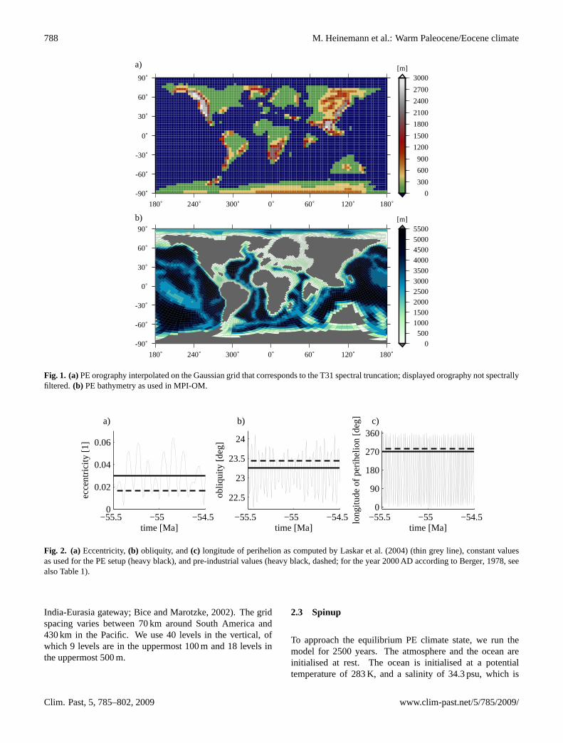
Orbital parameters in our PE simulation are set to constantvalues (see Table1). The longitude of perihelion, the obliq-uity, and the eccentricity as computed byLaskar et al.(2004)vary on timescales much shorter than the length of the PEperiod (Fig.2). Moreover,Laskar et al.(2004) reported thattheir simulation of the orbital parameters becomes uncertainfor more than 40 to 50 Ma ago. We select a longitude of per-ihelion such that the Northern Hemisphere winter occurs inthe aphelion (almost like today). The present-day obliquityand eccentricity are rather extreme values. For the PE, weselect an obliquity and an eccentricity closer to the temporalaverage of the solution byLaskar et al.(2004, see Fig.2).

2.2 Ocean-sea ice general circulation model

The Max-Planck-Institute Ocean Model (MPI-OM, here:version 1.2.0) is a z-coordinate global GCM based on theprimitive equations for a hydrostatic Boussinesq fluid witha free surface (Marsland et al., 2003). Scalar and vectorvariables are formulated on an orthogonal curvilinear C-grid(Arakawa and Lamb, 1977). Along-isopycnal diffusion isimplemented followingGriffies (1998). Horizontal tracermixing by unresolved eddies is parameterised followingGentet al.(1995). For the vertical eddy viscosity and diffusion theRichardson-number dependent scheme ofPacanowski andPhilander(1981) is applied. Since the Pacanowski-Philander(PP) scheme in its classical form underestimates the turbu-lent mixing close to the surface, an additional wind mixingparameterisation is included. In the presence of static in-stability, convective overturning is parameterised by greatlyenhanced vertical diffusion. A bottom boundary layer slopeconvection scheme allows for an improved representation ofthe flow of statically unstable dense water over sills. The ef-fect of ocean currents on surface wind stress is accountedfor following Luo et al. (2005). The embedded sea icemodel consists of sea ice dynamics followingHibler (1979)and zero-dimensional thermodynamics followingSemtner(1976). For more details on MPI-OM and the embeddedsea ice model seeMarsland et al.(2003) andJungclaus et al.(2006).

To apply MPI-OM to the PE, we include the PEbathymetry and generate an appropriate model grid. As forthe orography in the atmospheric model, we interpolate thebathymetry from the reconstruction byBice and Marotzke(2001). The MPI-OM grid structure allows for an arbitraryplacement of the grid poles; we generate a grid with a grid-North Pole on Paleo-Asia and a grid-South Pole on Paleo-South America (Fig.1b). This model grid has several ad-vantages. Positioning the grid-poles over land removes thenumerical singularities associated with the convergence ofmeridians at the geographical poles. Positioning the grid-poles onwide landmasses allows us to reduce the total num-ber of gridpoints. Moreover, this setup yields a higher res-olution of many small but important seaways (e.g., openNorth Atlantic, Central American Seaway, Tethys Seaway,

www.clim-past.net/5/785/2009/ Clim. Past, 5, 785–802, 2009


180˚ 240˚ 300˚ 0˚ 60˚ 120˚ 180˚

-90˚

-60˚

-30˚

0˚

30˚

60˚

90˚

0

300

600

900

1200

1500

1800

2100

2400

2700

3000[m]

180˚ 240˚ 300˚ 0˚ 60˚ 120˚ 180˚

-90˚

-60˚

-30˚

0˚

30˚

60˚

90˚

0

500

1000

1500

2000

2500

3000

3500

4000

45005000

5500[m]b)

a)

Fig. 1. (a) PE orography interpolated on the Gaussian grid that corresponds to the T31 spectraltruncation; displayed orography not spectrally filtered. (b) PE bathymetry as used in MPI-OM.

33

Fig. 1. (a)PE orography interpolated on the Gaussian grid that corresponds to the T31 spectral truncation; displayed orography not spectrallyfiltered. (b) PE bathymetry as used in MPI-OM.

−55.5 −55 −54.50

0.02

0.04

0.06

a)

time [Ma]

ecce

ntri

city

[1]

−55.5 −55 −54.5

22.5

23

23.5

24

b)

time [Ma]

obliq

uity

[de

g]

−55.5 −55 −54.50

90

180

270

360c)

time [Ma]

long

itude

of

peri

helio

n [d

eg]

Fig. 2. (a)Eccentricity,(b) obliquity, and(c) longitude of perihelion as computed byLaskar et al.(2004) (thin grey line), constant valuesas used for the PE setup (heavy black), and pre-industrial values (heavy black, dashed; for the year 2000 AD according toBerger, 1978, seealso Table1).

India-Eurasia gateway;Bice and Marotzke, 2002). The gridspacing varies between 70 km around South America and430 km in the Pacific. We use 40 levels in the vertical, ofwhich 9 levels are in the uppermost 100 m and 18 levels inthe uppermost 500 m.

2.3 Spinup

To approach the equilibrium PE climate state, we run themodel for 2500 years. The atmosphere and the ocean areinitialised at rest. The ocean is initialised at a potentialtemperature of 283 K, and a salinity of 34.3 psu, which is



Table 1. ECHAM5 input parameters as used in the PE model setup compared to those in the pre-industrial reference run (PR); FAOdetermines volumetric heat capacity and thermal diffusivity of soil; note that, while the PE land surface is homogeneous, the land surfaceparameters for PR are spatially variable; the PR values given here are mean values. The pre-industrial orbital parameters are given for theyear 2000 AD according toBerger(1978) while, actually, the orbital parameters in PR vary temporally according to VSOP87 (VariationsSeculaire des Orbites Planetaires,Bretagnon and Francou, 1988).

parameter PE PR

carbon dioxide concentration (pCO2) 560 ppm 278 ppmmethane concentration (pCH4) 0.8 ppm 0.65 ppmnitrous oxide concentration (pN2O) 0.288 ppm 0.27 ppm

total solar irradiance (S0) 1367 W m−2 1367 W m−2

eccentricity of the Earth’s orbit 0.0300 0.0167obliquity or inclination of the Earth’s axis 23.25o 23.44o

longitude of perihelion 270o 283o

land surface background albedo 0.16 0.25sea surface albedo 0.07 0.07vegetation ratio 0.6 0.4leaf area index (LAI) 2.3 2.2forest fraction 0.40 0.26maximum field capacity of soil (single bucket water height) 1.2 m 0.6 mFAO soil data flag (1∼sand, 3∼mud, 5∼clay) 3 2.6surface roughness length over land 1.6 m 1.6 m

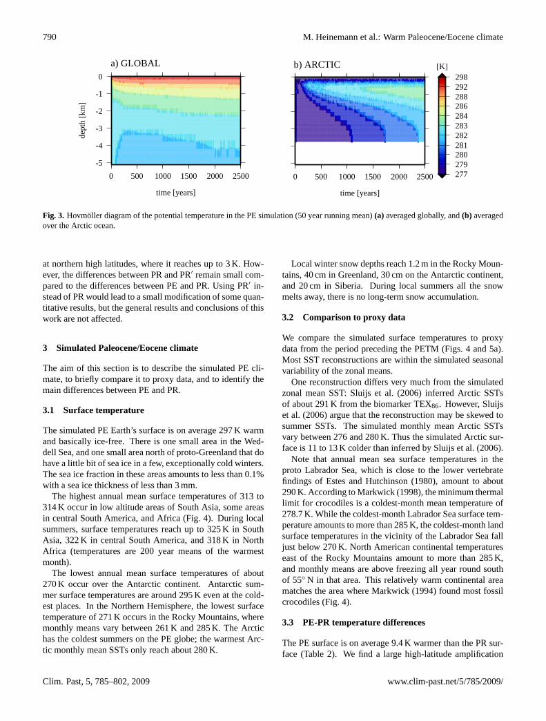
approximately the salinity we would get in the present-dayocean if all glaciers melted completely. The atmosphere ap-proaches its equilibrium after some 150 years, whereas inmost ocean basins the transient phase lasts for about 1000years. After 1000 years, the globally averaged temperatureseven at the deepest levels only increase by less than 0.3 K per1000 years (Fig.3a).

The Arctic deep ocean takes especially long to equilibrate,since it is only connected to the other basins via shallow sills.Moreover, the Arctic is stratified due to fresh surface wa-ter that inhibits vertical mixing. After 2000 years, the Arcticdeep ocean is 281 to 283 K warm and still warming by morethan 1 K per 1000 years (Fig.3b). The Arctic SST hardlyshows a warming trend, despite the deep ocean warming.

2.4 Pre-industrial reference simulation

In this study, we compare the PE simulation to a 2200 yearlong ECHAM5/MPI-OM simulation with pre-industrialboundary conditions that has been initialised from Levi-tus data. We refer to this pre-industrial reference simula-tion as PR. The pre-industrial boundary conditions includethe bathymetry, orography, greenhouse gas concentrations,soil and vegetation properties, and orbital parameters (Ta-ble 1). The pre-industrial boundary conditions also includethe subgrid-scale orographic information; the SSO parame-terisation in PR is switched on, while it is switched off inPE. Moreover, PR uses a modified physical parameterisationof friction and diffusion to improve the representation of theEl Nino-Southern Oscillation (ENSO, seeJungclaus et al.,

2006), while PE uses the standard MPI-OM parameter set-tings as specified byMarsland et al.(2003). While the orbitalparameters in PE are constant, the parameters in PR varytemporally according to VSOP87 (Variations Seculaire desOrbites Planetaires,Bretagnon and Francou, 1988, the firstyear of PR is 800 AD, the last year is 2999 AD). The philos-ophy behind this approach is to compare the PE simulationto an as good as possible representation of the pre-industrialclimate.

An alternative approach to set up a pre-industrial referencewould be to degrade the pre-industrial boundary conditionsto the level of accuracy available for the PE (see, e.g.,Hu-ber et al., 2003), which would worsen the representation ofthe pre-industrial climate. Such a degradation would alsoinclude to switch off the SSO parameterisation. To test theeffect of the SSO parameterisation, and to ensure that neitherthe ENSO-tuning nor the dynamic orbital parameters havea major effect on the pre-industrial climate, we perform a400 year long pre-industrial sensitivity run. This sensitivityrun (PR′) restarts from PR, it does not use the SSO parame-terisation nor the ENSO-tuning, and it uses constant orbitalparameters as specified in Table1. Moreover, it uses thePE concentrations of nitrous oxide and methane (Table1),and a carbon dioxide concentration of 280 ppm (instead of278 ppm). Hence, the difference between PE and PR′ is theland-sea mask and topography, the vegetation, the (now con-stant as in PE) orbital forcing, and the (now exactly) dou-bledpCO2. We find that the differences in the model setupbetween PR and PR′ lead to a global warming of approxi-mately 0.8 K in PR′ compared to PR. The warming is largest



-5

-4

-3

-2

-1

0de

pth

[km

]

0 500 1000 1500 2000 2500

time [years]

277279280281282283284286288292298

[K]

-5

-4

-3

-2

-1

0

dept

h [k

m]

0 500 1000 1500 2000 2500

time [years]

277279280281282283284286288292298

[K]a) GLOBAL b) ARCTIC

Fig. 3. Hovmoller diagram of the potential temperature in the PE simulation (50 year runningmean) a) averaged globally, and b) averaged over the Arctic ocean.

35

Fig. 3. Hovmoller diagram of the potential temperature in the PE simulation (50 year running mean)(a) averaged globally, and(b) averagedover the Arctic ocean.

at northern high latitudes, where it reaches up to 3 K. How-ever, the differences between PR and PR′ remain small com-pared to the differences between PE and PR. Using PR′ in-stead of PR would lead to a small modification of some quan-titative results, but the general results and conclusions of thiswork are not affected.

3 Simulated Paleocene/Eocene climate

The aim of this section is to describe the simulated PE cli-mate, to briefly compare it to proxy data, and to identify themain differences between PE and PR.

3.1 Surface temperature

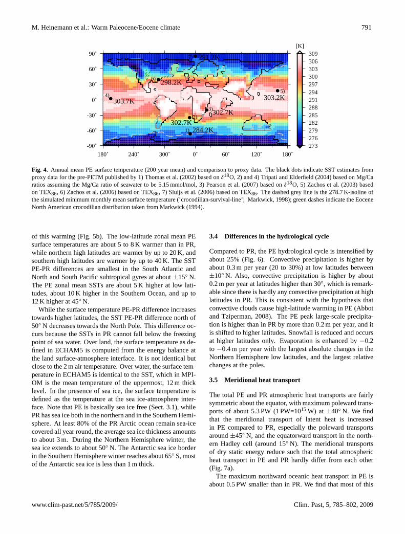
The simulated PE Earth’s surface is on average 297 K warmand basically ice-free. There is one small area in the Wed-dell Sea, and one small area north of proto-Greenland that dohave a little bit of sea ice in a few, exceptionally cold winters.The sea ice fraction in these areas amounts to less than 0.1%with a sea ice thickness of less than 3 mm.

The highest annual mean surface temperatures of 313 to314 K occur in low altitude areas of South Asia, some areasin central South America, and Africa (Fig.4). During localsummers, surface temperatures reach up to 325 K in SouthAsia, 322 K in central South America, and 318 K in NorthAfrica (temperatures are 200 year means of the warmestmonth).

The lowest annual mean surface temperatures of about270 K occur over the Antarctic continent. Antarctic sum-mer surface temperatures are around 295 K even at the cold-est places. In the Northern Hemisphere, the lowest surfacetemperature of 271 K occurs in the Rocky Mountains, wheremonthly means vary between 261 K and 285 K. The Arctichas the coldest summers on the PE globe; the warmest Arc-tic monthly mean SSTs only reach about 280 K.

Local winter snow depths reach 1.2 m in the Rocky Moun-tains, 40 cm in Greenland, 30 cm on the Antarctic continent,and 20 cm in Siberia. During local summers all the snowmelts away, there is no long-term snow accumulation.

3.2 Comparison to proxy data

We compare the simulated surface temperatures to proxydata from the period preceding the PETM (Figs.4 and5a).Most SST reconstructions are within the simulated seasonalvariability of the zonal means.

One reconstruction differs very much from the simulatedzonal mean SST:Sluijs et al.(2006) inferred Arctic SSTsof about 291 K from the biomarker TEX86. However,Sluijset al.(2006) argue that the reconstruction may be skewed tosummer SSTs. The simulated monthly mean Arctic SSTsvary between 276 and 280 K. Thus the simulated Arctic sur-face is 11 to 13 K colder than inferred bySluijs et al.(2006).

Note that annual mean sea surface temperatures in theproto Labrador Sea, which is close to the lower vertebratefindings of Estes and Hutchinson(1980), amount to about290 K. According toMarkwick (1998), the minimum thermallimit for crocodiles is a coldest-month mean temperature of278.7 K. While the coldest-month Labrador Sea surface tem-perature amounts to more than 285 K, the coldest-month landsurface temperatures in the vicinity of the Labrador Sea falljust below 270 K. North American continental temperatureseast of the Rocky Mountains amount to more than 285 K,and monthly means are above freezing all year round southof 55◦ N in that area. This relatively warm continental areamatches the area whereMarkwick (1994) found most fossilcrocodiles (Fig.4).

3.3 PE-PR temperature differences

The PE surface is on average 9.4 K warmer than the PR sur-face (Table2). We find a large high-latitude amplification



180˚ 240˚ 300˚ 0˚ 60˚ 120˚ 180˚

-90˚

-60˚

-30˚

0˚

30˚

60˚

90˚

273276279282285288291294297300303306309

[K]

284.2K1)

2)302.7K

302.7K3)

5)

6)

4)303.7K

298.2K

303.2K

291.2K7)

Fig. 4. Annual mean PE surface temperature (200 year mean) and comparison to proxy data.The black dots indicate SST estimates from proxy data for the pre-PETM published by 1)Thomas et al. (2002) based on δ18O, 2) and 4) Tripati and Elderfield (2004) based on Mg/Caratios assuming the Mg/Ca ratio of seawater to be 5.15 mmol/mol, 3) Pearson et al. (2007)based on δ18O, 5) Zachos et al. (2003) based on TEX86, 6) Zachos et al. (2006) based onTEX86, 7) Sluijs et al. (2006) based on TEX86. The dashed grey line is the 278.7 K-isoline ofthe simulated minimum monthly mean surface temperature (’crocodilian-survival-line’; Mark-wick, 1998); green dashes indicate the Eocene North American crocodilian distribution takenfrom Markwick (1994).

36

Fig. 4. Annual mean PE surface temperature (200 year mean) and comparison to proxy data. The black dots indicate SST estimates fromproxy data for the pre-PETM published by 1)Thomas et al.(2002) based onδ18O, 2) and 4)Tripati and Elderfield(2004) based on Mg/Caratios assuming the Mg/Ca ratio of seawater to be 5.15 mmol/mol, 3)Pearson et al.(2007) based onδ18O, 5) Zachos et al.(2003) basedon TEX86, 6) Zachos et al.(2006) based on TEX86, 7) Sluijs et al.(2006) based on TEX86. The dashed grey line is the 278.7 K-isoline ofthe simulated minimum monthly mean surface temperature (’crocodilian-survival-line’;Markwick, 1998); green dashes indicate the EoceneNorth American crocodilian distribution taken fromMarkwick (1994).

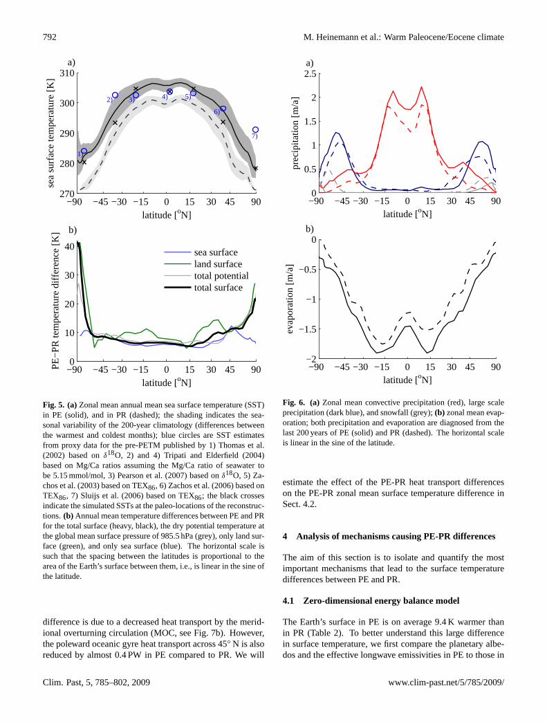
of this warming (Fig.5b). The low-latitude zonal mean PEsurface temperatures are about 5 to 8 K warmer than in PR,while northern high latitudes are warmer by up to 20 K, andsouthern high latitudes are warmer by up to 40 K. The SSTPE-PR differences are smallest in the South Atlantic andNorth and South Pacific subtropical gyres at about±15◦ N.The PE zonal mean SSTs are about 5 K higher at low lati-tudes, about 10 K higher in the Southern Ocean, and up to12 K higher at 45◦ N.

While the surface temperature PE-PR difference increasestowards higher latitudes, the SST PE-PR difference north of50◦ N decreases towards the North Pole. This difference oc-curs because the SSTs in PR cannot fall below the freezingpoint of sea water. Over land, the surface temperature as de-fined in ECHAM5 is computed from the energy balance atthe land surface-atmosphere interface. It is not identical butclose to the 2 m air temperature. Over water, the surface tem-perature in ECHAM5 is identical to the SST, which in MPI-OM is the mean temperature of the uppermost, 12 m thicklevel. In the presence of sea ice, the surface temperature isdefined as the temperature at the sea ice-atmosphere inter-face. Note that PE is basically sea ice free (Sect.3.1), whilePR has sea ice both in the northern and in the Southern Hemi-sphere. At least 80% of the PR Arctic ocean remain sea-icecovered all year round, the average sea ice thickness amountsto about 3 m. During the Northern Hemisphere winter, thesea ice extends to about 50◦ N. The Antarctic sea ice borderin the Southern Hemisphere winter reaches about 65◦ S, mostof the Antarctic sea ice is less than 1 m thick.

3.4 Differences in the hydrological cycle

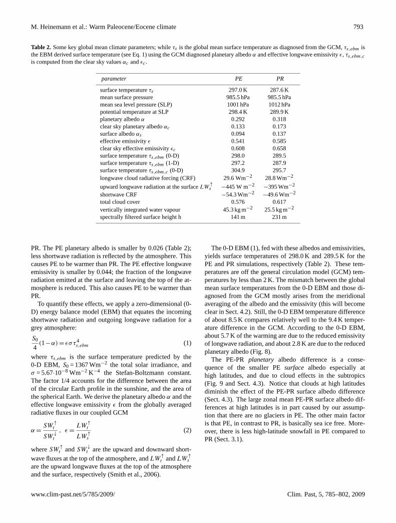
Compared to PR, the PE hydrological cycle is intensified byabout 25% (Fig.6). Convective precipitation is higher byabout 0.3 m per year (20 to 30%) at low latitudes between±10◦ N. Also, convective precipitation is higher by about0.2 m per year at latitudes higher than 30◦, which is remark-able since there is hardly any convective precipitation at highlatitudes in PR. This is consistent with the hypothesis thatconvective clouds cause high-latitude warming in PE (Abbotand Tziperman, 2008). The PE peak large-scale precipita-tion is higher than in PR by more than 0.2 m per year, and itis shifted to higher latitudes. Snowfall is reduced and occursat higher latitudes only. Evaporation is enhanced by−0.2to −0.4 m per year with the largest absolute changes in theNorthern Hemisphere low latitudes, and the largest relativechanges at the poles.

3.5 Meridional heat transport

The total PE and PR atmospheric heat transports are fairlysymmetric about the equator, with maximum poleward trans-ports of about 5.3 PW (1 PW=1015 W) at ±40◦ N. We findthat the meridional transport of latent heat is increasedin PE compared to PR, especially the poleward transportsaround±45◦ N, and the equatorward transport in the north-ern Hadley cell (around 15◦ N). The meridional transportsof dry static energy reduce such that the total atmosphericheat transport in PE and PR hardly differ from each other(Fig. 7a).

The maximum northward oceanic heat transport in PE isabout 0.5 PW smaller than in PR. We find that most of this



−90 −45 −30 −15 0 15 30 45 90270

280

290

300

310

latitude [oN]

sea

surf

ace

tem

pera

ture

[K

]a)

1)

2) 3) 4) 5)

6)

7)

−90 −45 −30 −15 0 15 30 45 900

10

20

30

40

latitude [oN]

PE−

PR te

mpe

ratu

re d

iffe

renc

e [K

] b)

sea surfaceland surfacetotal potentialtotal surface

Fig. 5. (a)Zonal mean annual mean sea surface temperature (SST)in PE (solid), and in PR (dashed); the shading indicates the sea-sonal variability of the 200-year climatology (differences betweenthe warmest and coldest months); blue circles are SST estimatesfrom proxy data for the pre-PETM published by 1)Thomas et al.(2002) based onδ18O, 2) and 4)Tripati and Elderfield(2004)based on Mg/Ca ratios assuming the Mg/Ca ratio of seawater tobe 5.15 mmol/mol, 3)Pearson et al.(2007) based onδ18O, 5) Za-chos et al.(2003) based on TEX86, 6) Zachos et al.(2006) based onTEX86, 7) Sluijs et al.(2006) based on TEX86; the black crossesindicate the simulated SSTs at the paleo-locations of the reconstruc-tions. (b) Annual mean temperature differences between PE and PRfor the total surface (heavy, black), the dry potential temperature atthe global mean surface pressure of 985.5 hPa (grey), only land sur-face (green), and only sea surface (blue). The horizontal scale issuch that the spacing between the latitudes is proportional to thearea of the Earth’s surface between them, i.e., is linear in the sine ofthe latitude.

difference is due to a decreased heat transport by the merid-ional overturning circulation (MOC, see Fig.7b). However,the poleward oceanic gyre heat transport across 45◦ N is alsoreduced by almost 0.4 PW in PE compared to PR. We will

−90 −45 −30 −15 0 15 30 45 900

0.5

1

1.5

2

2.5

latitude [oN]

prec

ipita

tion

[m/a

]

a)

−90 −45 −30 −15 0 15 30 45 90−2

−1.5

−1

−0.5

0

latitude [oN]

evap

orat

ion

[m/a

]

b)

Fig. 6. (a) Zonal mean convective precipitation (red), large scaleprecipitation (dark blue), and snowfall (grey);(b) zonal mean evap-oration; both precipitation and evaporation are diagnosed from thelast 200 years of PE (solid) and PR (dashed). The horizontal scaleis linear in the sine of the latitude.

estimate the effect of the PE-PR heat transport differenceson the PE-PR zonal mean surface temperature difference inSect.4.2.

4 Analysis of mechanisms causing PE-PR differences

The aim of this section is to isolate and quantify the mostimportant mechanisms that lead to the surface temperaturedifferences between PE and PR.

4.1 Zero-dimensional energy balance model

The Earth’s surface in PE is on average 9.4 K warmer thanin PR (Table2). To better understand this large differencein surface temperature, we first compare the planetary albe-dos and the effective longwave emissivities in PE to those in



Table 2. Some key global mean climate parameters; whileτs is the global mean surface temperature as diagnosed from the GCM,τs,ebm isthe EBM derived surface temperature (see Eq.1) using the GCM diagnosed planetary albedoα and effective longwave emissivityε, τs,ebm,c

is computed from the clear sky valuesαc andεc.

parameter PE PR

surface temperatureτs 297.0 K 287.6 Kmean surface pressure 985.5 hPa 985.5 hPamean sea level pressure (SLP) 1001 hPa 1012 hPapotential temperature at SLP 298.4 K 289.9 Kplanetary albedoα 0.292 0.318clear sky planetary albedoαc 0.133 0.173surface albedoαs 0.094 0.137effective emissivityε 0.541 0.585clear sky effective emissivityεc 0.608 0.658surface temperatureτs,ebm (0-D) 298.0 289.5surface temperatureτs,ebm (1-D) 297.2 287.9surface temperatureτs,ebm,c (0-D) 304.9 295.7longwave cloud radiative forcing (CRF) 29.6 Wm−2 28.8 Wm−2

upward longwave radiation at the surfaceLW↑s −445 W m−2

−395 Wm−2

shortwave CRF −54.3 Wm−2−49.6 Wm−2

total cloud cover 0.576 0.617vertically integrated water vapour 45.3 kg m−2 25.5 kg m−2

spectrally filtered surface height h 141 m 231 m

PR. The PE planetary albedo is smaller by 0.026 (Table2);less shortwave radiation is reflected by the atmosphere. Thiscauses PE to be warmer than PR. The PE effective longwaveemissivity is smaller by 0.044; the fraction of the longwaveradiation emitted at the surface and leaving the top of the at-mosphere is reduced. This also causes PE to be warmer thanPR.

To quantify these effects, we apply a zero-dimensional (0-D) energy balance model (EBM) that equates the incomingshortwave radiation and outgoing longwave radiation for agrey atmosphere:

S0

4(1−α) = εστ4

s,ebm (1)

where τs,ebm is the surface temperature predicted by the0-D EBM, S0 = 1367 Wm−2 the total solar irradiance, andσ = 5.67·10−8 Wm−2 K−4 the Stefan-Boltzmann constant.The factor 1/4 accounts for the difference between the areaof the circular Earth profile in the sunshine, and the area ofthe spherical Earth. We derive the planetary albedoα and theeffective longwave emissivityε from the globally averagedradiative fluxes in our coupled GCM

α =SW

↑

t

SW↓

t

, ε =LW

↑

t

LW↑s

(2)

whereSW↑

t andSW↓

t are the upward and downward short-wave fluxes at the top of the atmosphere, andLW

↑

t andLW↑s

are the upward longwave fluxes at the top of the atmosphereand the surface, respectively (Smith et al., 2006).

The 0-D EBM (1), fed with these albedos and emissivities,yields surface temperatures of 298.0 K and 289.5 K for thePE and PR simulations, respectively (Table2). These tem-peratures are off the general circulation model (GCM) tem-peratures by less than 2 K. The mismatch between the globalmean surface temperatures from the 0-D EBM and those di-agnosed from the GCM mostly arises from the meridionalaveraging of the albedo and the emissivity (this will becomeclear in Sect.4.2). Still, the 0-D EBM temperature differenceof about 8.5 K compares relatively well to the 9.4 K temper-ature difference in the GCM. According to the 0-D EBM,about 5.7 K of the warming are due to the reduced emissivityof longwave radiation, and about 2.8 K are due to the reducedplanetary albedo (Fig.8).

The PE-PR planetary albedo difference is a conse-quence of the smaller PEsurface albedo especially athigh latitudes, and due to cloud effects in the subtropics(Fig. 9 and Sect.4.3). Notice that clouds at high latitudesdiminish the effect of the PE-PR surface albedo difference(Sect.4.3). The large zonal mean PE-PR surface albedo dif-ferences at high latitudes is in part caused by our assump-tion that there are no glaciers in PE. The other main factoris that PE, in contrast to PR, is basically sea ice free. More-over, there is less high-latitude snowfall in PE compared toPR (Sect.3.1).



−90 −45 −30 −15 0 15 30 45 90−6

−4

−2

0

2

4

6

dry

latent

total

latitude [oN]

atm

osph

ere

heat

tran

spor

t [PW

]

a)

−90 −45 −30 −15 0 15 30 45 90−3

−2

−1

0

1

2

3

gyre

MOC

total

latitude [oN]

ocea

n he

at tr

ansp

ort [

PW]

b)

Fig. 7. (a)Zonally integrated meridional heat transport in the atmo-sphere due to the advection of dry air (green), due to the advectionof moisture/latent heat (blue), and the sum (black), for PE (solid)and PR (dashed), computed from the last 100 years of each runwith 6 hourly instantaneous sampling;(b) zonally integrated merid-ional ocean heat transport due to the meridional overturning circu-lation (MOC, blue), due to the gyre circulation (green), and the sum(black), for PE (solid) and PR (dashed), computed from monthlymeans of the last 1000 years of each run. The horizontal scale islinear in the sine of the latitude.

4.2 One-dimensional energy balance model

To assess the effect of the latitudinal inhomogeneity of theemissivity, albedo, and heat transport differences between PEand PR (Figs.7 and9), we extend the 0-D EBM (1) to themeridional dimension:

SW↓

t (φ)[1−α(φ)]−1

2πR2cosφ

∂F(φ)

∂φ= ε(φ)στ4

s,ebm(φ)(3)

whereφ is the latitude,R the radius of the Earth,SW↓

t (φ) thezonal mean downward shortwave radiation at the top of theatmosphere,α(φ) the zonal mean planetary albedo,ε(φ) thezonal mean emissivity,F(φ) the total meridional heat trans-

warm

1K

cold287.6K

290K

297.0K

+2.

8K

+5.7K

+8.5K

0.33

0.32

0.31

0.3

0.29

0.560.540.52 0.58 0.6 0.62emissivity

plan

etar

y al

bedo

Fig. 8. Using the EBM to trace back the temperature difference be-tween PE and PR to albedo and emissivity changes in the GCM;grey lines are contour lines of the EBM-predicted temperature forcertain emissivities and albedos, contour intervals are 1K; the redand blue lines are the GCM-diagnosed temperatures for PE and PR,respectively; the circles are the surface temperatures predicted bythe EBM using the GCM-diagnosed emissivities and albedos; theblack arrow indicates the EBM-predicted PE-PR temperature dif-ference; the black lines are auxiliary lines to estimate the albedo-and emissivity-caused temperature difference separately.

port, andτs(φ) the one-dimensional (1-D) EBM-predictedzonal mean surface temperature.

As in Sect.4.1for the 0-D EBM, we now fit this 1-D EBMto the GCM simulations PE and PR. To this end, we diagnosethe zonal mean downward top-of-atmosphere shortwave ra-diation, the emissivity, and the albedo from the GCM simu-lations PE and PR, respectively. To compute the divergenceof the total meridional heat transport∂

∂φF(φ), we diagnose

the net shortwave plus longwave radiative flux at the top ofthe atmosphere; in other words, we compute the implied at-mosphere plus ocean meridional heat transport divergence:

∂F (φ)

∂φ= −2πR2cosφ(SWnet

t (φ)+LWnett (φ)) (4)

where SWnett (φ) and LWnet

t (φ) are the zonal mean net(downward is positive) top-of-atmosphere shortwave andlongwave radiative fluxes, respectively.

We apply these diagnosed emissivities, albedos, and heatfluxes to the 1-D EBM to compute the zonal mean sur-face temperaturesτs,ebm(φ) for PE and PR, respectively.The resulting 1-D EBM-predicted zonal mean PE and



−90 −45 −30 −15 0 15 30 45 900

0.2

0.4

0.6

0.8

latitude [oN]

albe

do [

1]

surface

planetary

a)

−90 −45 −30 −15 0 15 30 45 900.4

0.5

0.6

0.7

0.8

0.9

latitude [oN]

long

wav

e em

issi

vity

[1]

b)

−90 −45 −30 −15 0 15 30 45 90

−0.25

−0.2

−0.15

−0.1

−0.05

0

0.05

latitude [oN]

PE−

PR e

mis

sivi

ty d

iffe

renc

e [1

]

total

due to clouds

c)

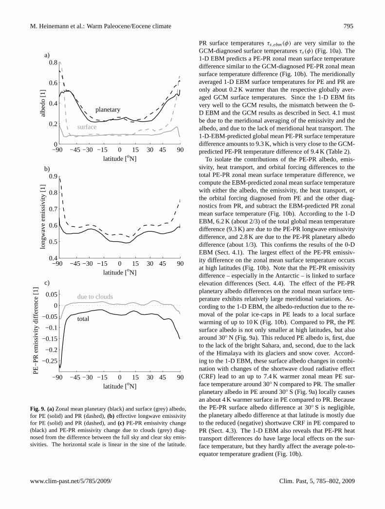
Fig. 9. (a)Zonal mean planetary (black) and surface (grey) albedo,for PE (solid) and PR (dashed),(b) effective longwave emissivityfor PE (solid) and PR (dashed), and(c) PE-PR emissivity change(black) and PE-PR emissivity change due to clouds (grey) diag-nosed from the difference between the full sky and clear sky emis-sivities. The horizontal scale is linear in the sine of the latitude.

PR surface temperaturesτs,ebm(φ) are very similar to theGCM-diagnosed surface temperaturesτs(φ) (Fig. 10a). The1-D EBM predicts a PE-PR zonal mean surface temperaturedifference similar to the GCM-diagnosed PE-PR zonal meansurface temperature difference (Fig.10b). The meridionallyaveraged 1-D EBM surface temperatures for PE and PR areonly about 0.2 K warmer than the respective globally aver-aged GCM surface temperatures. Since the 1-D EBM fitsvery well to the GCM results, the mismatch between the 0-D EBM and the GCM results as described in Sect.4.1 mustbe due to the meridional averaging of the emissivity and thealbedo, and due to the lack of meridional heat transport. The1-D-EBM-predicted global mean PE-PR surface temperaturedifference amounts to 9.3 K, which is very close to the GCM-predicted PE-PR temperature difference of 9.4 K (Table2).

To isolate the contributions of the PE-PR albedo, emis-sivity, heat transport, and orbital forcing differences to thetotal PE-PR zonal mean surface temperature difference, wecompute the EBM-predicted zonal mean surface temperaturewith either the albedo, the emissivity, the heat transport, orthe orbital forcing diagnosed from PE and the other diag-nostics from PR, and subtract the EBM-predicted PR zonalmean surface temperature (Fig.10b). According to the 1-DEBM, 6.2 K (about 2/3) of the total global mean temperaturedifference (9.3 K) are due to the PE-PR longwave emissivitydifference, and 2.8 K are due to the PE-PR planetary albedodifference (about 1/3). This confirms the results of the 0-DEBM (Sect.4.1). The largest effect of the PE-PR emissiv-ity difference on the zonal mean surface temperature occursat high latitudes (Fig.10b). Note that the PE-PR emissivitydifference – especially in the Antarctic – is linked to surfaceelevation differences (Sect.4.4). The effect of the PE-PRplanetary albedo differences on the zonal mean surface tem-perature exhibits relatively large meridional variations. Ac-cording to the 1-D EBM, the albedo-reduction due to the re-moval of the polar ice-caps in PE leads to a local surfacewarming of up to 10 K (Fig.10b). Compared to PR, the PEsurface albedo is not only smaller at high latitudes, but alsoaround 30◦ N (Fig. 9a). This reduced PE albedo is, first, dueto the lack of the bright Sahara, and, second, due to the lackof the Himalaya with its glaciers and snow cover. Accord-ing to the 1-D EBM, these surface albedo changes in combi-nation with changes of the shortwave cloud radiative effect(CRF) lead to an up to 7.4 K warmer zonal mean PE sur-face temperature around 30◦ N compared to PR. The smallerplanetary albedo in PE around 30◦ S (Fig.9a) locally causesan about 4 K warmer surface in PE compared to PR. Becausethe PE-PR surface albedo difference at 30◦ S is negligible,the planetary albedo difference at that latitude is mostly dueto the reduced (negative) shortwave CRF in PE compared toPR (Sect.4.3). The 1-D EBM also reveals that PE-PR heattransport differences do have large local effects on the sur-face temperature, but they hardly affect the average pole-to-equator temperature gradient (Fig.10b).



−90 −45 −30 −15 0 15 30 45 90

240

260

280

300

latitude [oN]

surf

ace

tem

pera

ture

[K

]a)

GCM PEGCM PREBM PEEBM PR

−90 −45 −30 −15 0 15 30 45 90

0

10

20

30

40

latitude [oN]PE−

PR s

urfa

ce te

mpe

ratu

re d

iffe

renc

e [K

]

b)

GCMEBMdue to PE emissivitydue to PE albedodue to PE heat transportdue to PE orbital parameters

Fig. 10. (a)Zonal mean surface temperatures for PE (solid) andPR (dashed) as computed with the 1-D EBM (red) and directly di-agnosed from the GCM (black).(b) Zonal mean PE-PR surfacetemperature difference as diagnosed from the GCM (black), andas computed from the 1-D EBM (red); the blue, green, grey, andorange lines indicate the temperature differences due to the PE-PR emissivity difference, the planetary albedo difference, the heattransport difference, and the orbital forcing difference, respectively,computed using the 1-D EBM (3).

4.3 Cloud radiative effect

To estimate the effect of clouds in both GCM simulations,we first apply the 0-D EBM (1). This time, however, we usetheclear skyradiative fluxes to compute the clear sky albedoαc and clear sky effective longwave emissivityεc

αc =SW

↑

t,c

SW↓

t

, εc =LW

↑

t,c

LW↑s

(5)

whereSW↑

t,c is the upward clear sky shortwave flux, and

LW↑

t,c is the upward clear sky longwave flux at the top of the

atmosphere. Note that the surface emits longwave radiationdepending on the surface temperature, no matter what thecloudiness. The clear sky fluxes in ECHAM5 are computedassuming that there are no clouds; the difference between thealbedos / emissivities computed from the clear sky and fullsky fluxes thus yields the effect of clouds.

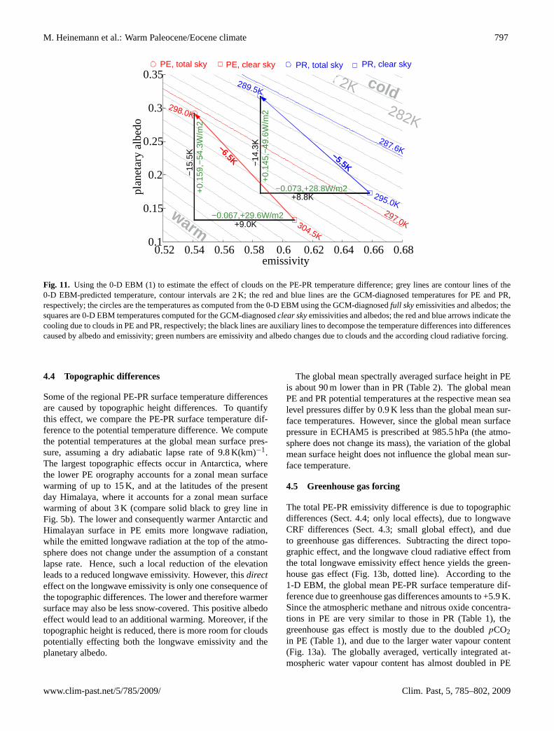
We find that clouds cause a 1 K stronger cooling in PEthan in PR (namely 6.5 K compared to 5.5 K, see Fig.11).The reason for this stronger cooling is that clouds in PEhave a larger effect on the albedo than clouds in PR. Theplanetary albedo increase due to clouds amounts to 0.159 inPE and only 0.145 in PR. By multiplication withS0/4, thistranslates into a shortwave CRF of−54.3 Wm−2 in PE com-pared to−49.6 Wm−2 in PR. Note that this larger negativeshortwave CRF in PE occurs despite a reduced total cloudcover (Table2). Even though the cloud cover is reduced,the shortwave effect of the clouds is larger in PE becausethe surface is darker. According to the 0-D EBM, the PEshortwave CRF causes a cooling of 15.0 or 15.5 K, depend-ing on whether we change the albedo or the emissivity first(black auxiliary lines in Fig.11are only drawn for emissivitydecrease first). The pre-industrial shortwave CRF causes acooling of 13.9 or 14.3 K. The difference of 0.7 to 1.6 K is re-duced by about 0.2 K due to a larger positive longwave CRFfor PE (29.6 Wm−2 compared to 28.8 Wm−2). This largerlongwave CRF in PE occurs despite a smaller cloud-inducedemissivity change in PE compared to PR, because the abso-lute amount of longwave radiation emitted from the surfaceis much larger in PE than in PR (445 Wm−2 compared to395 Wm−2, Table2).

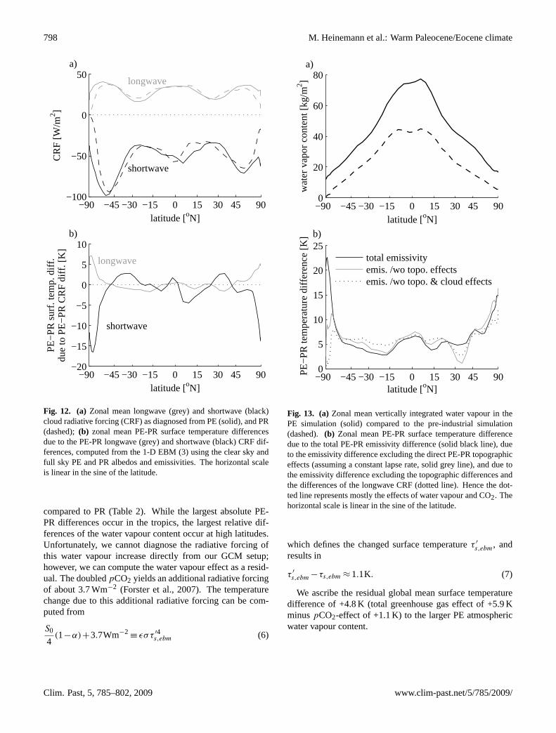
Note that the global mean PE-PR emissivity difference dueto cloud cover differences is small only because the largeremissivity-effect of clouds at high latitudes in PE comparedto PR is compensated by a smaller emissivity-effect of cloudsat low latitudes (grey line in Fig.9c). According to the 1-DEBM, the larger high-latitude and smaller low-latitude long-wave CRF in PE compared to PR (Fig.12a) lead to a reduc-tion of the pole-to-equator temperature gradient by about 5 K(Fig. 12b).

On the other hand, clouds reduce the effect of the largehigh-latitude PE-PR surface albedo difference (Fig.9a). Thenegative shortwave CRF at high latitudes in PE is larger thanin PR, which, according to the 1-D EBM, causes the PE highlatitudes to be up to 15 K colder than the PR high latitudes(Fig. 12b). Even though the surface albedo in the subtropicsespecially in the Southern Hemisphere in PE hardly differsfrom that in PR, the planetary albedo in the subtropics is sig-nificantly smaller in PE than in PR (Figure9a). This smallersubtropical shortwave CRF in PE compared to PR (Fig.12a)leads to almost 3 K warmer subtropics in PE compared to PR(Fig. 12b).



warm

2K cold

287.6K

282K298.0K

289.5K

−5.5K

−6.5K

−14

.3K

−15

.5K

304.5K

297.0K

295.0K+

0.15

9,−

54.3

W/m

2

+0.

145,

−49

.6W

/m2

+9.0K−0.067,+29.6W/m2

−0.073,+28.8W/m2

0.2

0.15

0.1

0.25

0.3

0.35

0.52 0.56 0.58 0.6 0.62 0.64 0.66 0.68emissivity

plan

etar

y al

bedo

0.54

+8.8K

PR, clear skyPR, total skyPE, clear skyPE, total sky

Fig. 11. Using the 0-D EBM (1) to estimate the effect of clouds on the PE-PR temperature difference; grey lines are contour lines of the0-D EBM-predicted temperature, contour intervals are 2 K; the red and blue lines are the GCM-diagnosed temperatures for PE and PR,respectively; the circles are the temperatures as computed from the 0-D EBM using the GCM-diagnosedfull skyemissivities and albedos; thesquares are 0-D EBM temperatures computed for the GCM-diagnosedclear skyemissivities and albedos; the red and blue arrows indicate thecooling due to clouds in PE and PR, respectively; the black lines are auxiliary lines to decompose the temperature differences into differencescaused by albedo and emissivity; green numbers are emissivity and albedo changes due to clouds and the according cloud radiative forcing.

4.4 Topographic differences

Some of the regional PE-PR surface temperature differencesare caused by topographic height differences. To quantifythis effect, we compare the PE-PR surface temperature dif-ference to the potential temperature difference. We computethe potential temperatures at the global mean surface pres-sure, assuming a dry adiabatic lapse rate of 9.8 K(km)−1.The largest topographic effects occur in Antarctica, wherethe lower PE orography accounts for a zonal mean surfacewarming of up to 15 K, and at the latitudes of the presentday Himalaya, where it accounts for a zonal mean surfacewarming of about 3 K (compare solid black to grey line inFig. 5b). The lower and consequently warmer Antarctic andHimalayan surface in PE emits more longwave radiation,while the emitted longwave radiation at the top of the atmo-sphere does not change under the assumption of a constantlapse rate. Hence, such a local reduction of the elevationleads to a reduced longwave emissivity. However, thisdirecteffect on the longwave emissivity is only one consequence ofthe topographic differences. The lower and therefore warmersurface may also be less snow-covered. This positive albedoeffect would lead to an additional warming. Moreover, if thetopographic height is reduced, there is more room for cloudspotentially effecting both the longwave emissivity and theplanetary albedo.

The global mean spectrally averaged surface height in PEis about 90 m lower than in PR (Table2). The global meanPE and PR potential temperatures at the respective mean sealevel pressures differ by 0.9 K less than the global mean sur-face temperatures. However, since the global mean surfacepressure in ECHAM5 is prescribed at 985.5 hPa (the atmo-sphere does not change its mass), the variation of the globalmean surface height does not influence the global mean sur-face temperature.

4.5 Greenhouse gas forcing

The total PE-PR emissivity difference is due to topographicdifferences (Sect.4.4; only local effects), due to longwaveCRF differences (Sect.4.3; small global effect), and dueto greenhouse gas differences. Subtracting the direct topo-graphic effect, and the longwave cloud radiative effect fromthe total longwave emissivity effect hence yields the green-house gas effect (Fig.13b, dotted line). According to the1-D EBM, the global mean PE-PR surface temperature dif-ference due to greenhouse gas differences amounts to +5.9 K.Since the atmospheric methane and nitrous oxide concentra-tions in PE are very similar to those in PR (Table1), thegreenhouse gas effect is mostly due to the doubledpCO2in PE (Table1), and due to the larger water vapour content(Fig. 13a). The globally averaged, vertically integrated at-mospheric water vapour content has almost doubled in PE



−90 −45 −30 −15 0 15 30 45 90−100

−50

0

50

latitude [oN]

CR

F [W

/m2 ]

longwave

shortwave

a)

−90 −45 −30 −15 0 15 30 45 90−20

−15

−10

−5

0

5

10

longwave

shortwave

latitude [oN]

PE−

PR s

urf.

tem

p. d

iff.

due

to P

E−

PR C

RF

diff

. [K

]

b)

Fig. 12. (a) Zonal mean longwave (grey) and shortwave (black)cloud radiative forcing (CRF) as diagnosed from PE (solid), and PR(dashed);(b) zonal mean PE-PR surface temperature differencesdue to the PE-PR longwave (grey) and shortwave (black) CRF dif-ferences, computed from the 1-D EBM (3) using the clear sky andfull sky PE and PR albedos and emissivities. The horizontal scaleis linear in the sine of the latitude.

compared to PR (Table2). While the largest absolute PE-PR differences occur in the tropics, the largest relative dif-ferences of the water vapour content occur at high latitudes.Unfortunately, we cannot diagnose the radiative forcing ofthis water vapour increase directly from our GCM setup;however, we can compute the water vapour effect as a resid-ual. The doubledpCO2 yields an additional radiative forcingof about 3.7 Wm−2 (Forster et al., 2007). The temperaturechange due to this additional radiative forcing can be com-puted from

S0

4(1−α)+3.7Wm−2

≡ εστ ′4s,ebm (6)

−90 −45 −30 −15 0 15 30 45 900

20

40

60

80

latitude [oN]

wat

er v

apor

con

tent

[kg

/m2 ]

a)

−90 −45 −30 −15 0 15 30 45 900

5

10

15

20

25

latitude [oN]

PE−

PR te

mpe

ratu

re d

iffe

renc

e [K

] b)

total emissivityemis. /wo topo. effectsemis. /wo topo. & cloud effects

Fig. 13. (a)Zonal mean vertically integrated water vapour in thePE simulation (solid) compared to the pre-industrial simulation(dashed). (b) Zonal mean PE-PR surface temperature differencedue to the total PE-PR emissivity difference (solid black line), dueto the emissivity difference excluding the direct PE-PR topographiceffects (assuming a constant lapse rate, solid grey line), and due tothe emissivity difference excluding the topographic differences andthe differences of the longwave CRF (dotted line). Hence the dot-ted line represents mostly the effects of water vapour and CO2. Thehorizontal scale is linear in the sine of the latitude.

which defines the changed surface temperatureτ ′

s,ebm, andresults in

τ ′

s,ebm −τs,ebm ≈ 1.1K. (7)

We ascribe the residual global mean surface temperaturedifference of +4.8 K (total greenhouse gas effect of +5.9 KminuspCO2-effect of +1.1 K) to the larger PE atmosphericwater vapour content.



−90 −45 −30 −15 0 15 30 45 90JF

MAMJJ

ASONDJ

−15

−12

−9

−9

−6

−6

−6

−6

−3

−3

−3 −3 −3

0

0 3

3

6

6

00

9

9

3 3

6 6

12

0

9

latitude [oN]

time

a)

−18−15−12−9 −6 −3 0 3 6 9 12 15

−90 −45 −30 −15 0 15 30 45 90−2

−1.5

−1

−0.5

0

0.5

1

latitude [oN]

PE−

PR S

Wt↓ d

iffe

renc

e [W

/m2 ]

b)

Fig. 14. (a)Seasonal cycle of the difference of the zonal mean incoming shortwave radiation at the top of the atmosphere between PE andPR; red indicates more incoming radiation in PE, blue indicates less radiation in PE. Contour intervals are 3 Wm−2. The incoming shortwaveradiation in PR is averaged over the last 200 years, i.e. over the years 2800 to 2999 AD.(b) Annual average of the PE-PR incoming shortwaveradiation difference. The horizontal scale is linear in the sine of the latitude.

4.6 Solar and orbital forcing

The choice of the orbital parameters as described in Sect.2leads to the following changes in PE, compared to PR: lessincoming shortwave radiation in the Northern Hemispherein May, June, and July; less incoming radiation in the Arc-tic spring and autumn; and more radiation mostly duringDecember and January at low and mid latitudes (Fig.14a).Integrated over the annual cycle, this amounts to about0.4 Wm−2 more incoming shortwave radiation at low andmiddle latitudes in PE, and about 1 Wm−2 less incomingshortwave radiation at high latitudes (Fig.14b). This re-distribution of the incoming shortwave radiation at the topof the atmosphere, from high latitudes to low latitudes, isdue to the smaller obliquity in PE compared to PR (Fig.2).According to the 1-D EBM, the PE-PR obliquity differenceleads to a maximum PE-PR temperature difference of about+0.1 K around 30◦ N, and to a PE-PR temperature differenceof about−0.2 K and less than−0.1 K at the South Pole andthe North Pole, respectively (Fig.10b, orange line). The re-sulting PE-PR global mean surface temperature difference ofless than +0.03 K due to the PE-PR obliquity difference isnegligible compared to the longwave emissivity and albedoeffects.

From the theory of stellar evolution, it is known that theSun has gradually brightened by more than 30% since it set-tled down to steady nuclear burning of hydrogen roughly4.5 billion years ago (Endal and Sofia, 1981; Peltier, 2003).Due to this brightening, the total solar irradiance 55 Ma agowas up to 0.6% (about 8 Wm−2) smaller than at present. Ac-cording to the 0-D EBM (1), and given the PE albedos andemissivities, the temperature change due to such a reductionof the radiative forcing would amount to less than−0.5 K.

5 Discussion and conclusions

Using the coupled atmosphere-ocean-sea ice general circu-lation model ECHAM5/MPI-OM, we perform a long, stableclimate simulation for the late Paleocene/early Eocene (PE).The simulated PE Earth surface is on average 297 K warmand ice-free. To our knowledge, we have obtained the firstcoupled PE simulation with moderate GHG forcing that iswarm enough at high latitudes to keep the poles free fromsea ice, while reasonably matching the lower latitude SSTreconstructions. However, if we take the SST proxy data bySluijs et al.(2006) at face value, the simulated Arctic surfacetemperature is still too cold.

A possible shortcoming of this study is the assumption ofa globally homogeneous vegetation. Including a more re-alistic vegetation distribution such as the one reconstructedby Utescher and Mosbrugger(2007) may, at least regionally,affect the climate (Sewall et al., 2000). Also, we did not in-clude lakes in our PE model setup. Including lakes (e.g., theNorth American Green River lake system) could lead to a fur-ther reduction of the seasonality in the continental interiors(Sloan, 1994).

We find that thetotal atmospheric heat transports in PEand the pre-industrial reference (PR) are very similar, al-though the latent heat fraction is larger in PE than in PR.The total poleward heat transport by the ocean is smaller inPE compared to PR. We conclude that meridional heat trans-ports do not contribute to the more equable PE climate inour simulation (confirming the results ofHuber and Sloan,2001). A more detailed analysis of the PE ocean circulationwill be subject of a future study.

Compared to PR, the simulated PE Earth surface is on av-erage 9.4 K warmer. While low latitudes in PE comparedto PR are on average about 5 to 8 K warmer, northern high



latitudes are warmer by up to 20 K, and southern high lat-itudes are warmer by up to 40 K. As diagnostic tools toroughly understand this temperature difference, we fit a 0-D EBM, and a 1-D EBM to the PE and PR GCM solutions.

According to the EBMs, one third of the PE-PR surfacetemperature difference is due to a reduced planetary albedo.The surface albedo in PE compared to PR is reduced mostlydue to the lack of glaciers, the lack of sea ice, and reducedsnowfall. However, this large high-latitude surface albedochange is partly compensated by a more negative shortwavecloud radiative forcing. In that sense, clouds in our PE modelwork against the high-latitude amplification of the snow andice albedo feedback. Nevertheless, the planetary albedo re-duction is largest at high latitudes.

Two thirds of the warming are due to a reduction of theeffective longwave emissivity. We find that clouds cause asignificant reduction of the effective longwave emissivity athigh latitudes. This reduction of the emissivity at high lat-itudes is overcompensated by an increase of the emissivitydue to clouds at lower latitudes. This way (via their effecton the longwave emissivity), clouds in PE compared to PRhardly affect the global mean temperature, but they cause apolar warming and a tropical cooling relative to PR.

The reduced orographic height in the PE setup does notdirectly affect the global mean temperature, but it does havelarge regional effects. Up to 15 K of the southern high-latitude PE-PR surface temperature difference are due to thelower Antarctic surface height in PE. The orographic differ-ences contribute to the high-latitude amplification of the clearsky PE-PR emissivity difference. We ascribe the largest frac-tion of the clear sky emissivity-induced PE-PR surface tem-perature difference to the water vapour feedback.

As a consequence of the reduced obliquity in our PE setup,a small amount of incoming shortwave radiation at the top ofthe atmosphere is redistributed from high latitudes to low lat-itudes. The resulting annual mean reduction of the radiativeforcing in PE compared to PR by about 1 Wm−2 at high lat-itudes leads to a negligible increase of the pole-to-equatortemperature gradient in the PE simulation compared to PR.

The PE simulation presented here is closer to proxyrecords than the previously published coupled Eocenesimulations byHuber and Sloan(2001) using the NationalCenter for Atmospheric Research (NCAR) Climate SystemModel (CSM) version 1.4, and byShellito et al.(2009) us-ing the NCAR Community Climate System Model (CCSM)version 3. We cannot ultimately say why this PE simu-lation is closer to proxy records than the previous simula-tions. There are many poorly constrained parameters thatmay have a large effect on the model solution; greenhousegases, land surface, vegetation, and soil parameters are ob-vious examples. We do not know all of these parametersfrom Huber and Sloan(2001) nor fromShellito et al.(2009),but assuming that the boundary conditions in the previousCSM1.4 and CCSM3 setups were similar to those we usehere, CSM1.4 and CCSM3 must have a smaller sensitivity

than ECHAM5/MPI-OM with respect to the PE-PR bound-ary condition differences. This smaller sensitivity with re-spect to the PE boundary conditions (including thepCO2-doubling) would be in line with the smaller climate sensi-tivity to a pCO2-doubling alone of the NCAR models com-pared to ECHAM5/MPI-OM (Kiehl et al., 2006; Randallet al., 2007). One way to analyse the differences betweenour PE simulation and the previous NCAR Eocene simu-lations would be to also apply the EBM analysis describedhere to the NCAR runs. We speculate that especially the wa-ter vapour feedback in our simulation is larger than in theNCAR simulations. An explicit investigation of thepCO2-sensitivity of our PE model solution will be subject of a fu-ture study.

Summing up, the warm and equable PE climate as sim-ulated in ECHAM5/MPI-OM is in part due to the smallersurface albedo compared to the pre-industrial reference, butmostly due to a smaller effective longwave emissivity es-pecially at high latitudes as a consequence of topographiceffects, cloud effects, and increased CO2 and water vapourconcentrations.

Acknowledgements.We thank Helmuth Haak for his help settingup the PE model, and for providing the pre-industrial referencesimulation. We thank Karen Bice for advice, and for providingthe paleo-topography. We thank three anonymous referees fortheir productive and helpful comments. We would like to thankDorian Abbot for discussions, and in particular for his suggestionto extend the 0-D EBM analysis in the meridional direction. Themodel experiments were carried out on the supercomputing systemof the German Climate Computation Centre (DKRZ) Hamburg.This work was completed during a Gary C. Comer Science andEducation Foundation Abrupt Climate Change Fellowship.

The service charges for this open access publication havebeen covered by the Max Planck Society.

Edited by: V. Rath

References

Abbot, D. S. and Tziperman, E.: Sea ice, high-latitude convection,and equable climates, Geophys. Res. Lett., 35, 1–5, 2008.

Alley, R. B., Marotzke, J., Nordhaus, W., Overpeck, J., Peteet, D.,Pielke Jr., R., Pierrehumbert, R., Rhines, P., Stocker, T., Talley,L., and Wallace, J. M.: Abrupt Climate Change: Inevitable Sur-prises, Natl. Acad. Press, 2002.

Arakawa, A. and Lamb, V. R.: Computational design of the ba-sic dynamical processes of the CLA general circulation model,Meth. Comput. Phys., 17, 173–265, 1977.

Barron, E. J.: Eocene equator-to-pole surface ocean temperatures:a significant climate problem?, Paleoceanography, 2, 729–739,1987.

Berger, A. L.: Long Term Variations of Daily Insolation and Qua-ternary Climatic Changes, J. Atmos. Sci., 35, 2362–2367, 1978.



Bice, K. L. and Marotzke, J.: Numerical evidence against reversedthermohaline circulation in the warm Paleocene/Eocene ocean,J. Geophys. Res., 106, 11529–11542, 2001.

Bice, K. L. and Marotzke, J.: Could changing ocean cir-culation have destabilized methane hydrate at the Pale-ocene/Eocene boundary?, Paleoceanography, 17(2), 1018,doi:10.1029/2001PA000678, 2002.

Bretagnon, P. and Francou, G.: Planetary theories in rectangularand spherical variables – VSOP 87 solutions, Astron. Astrophys.,202, 309–315, 1988.

Covey, C. and Barron, E.: The Role of Ocean Heat Transport inClimatic Change, Earth Sci. Rev., 24, 429–445, 1988.

Dickens, G. R., O’Neil, J. R., Rea, D. K., and Owen, R. M.: Dis-sociation of oceanic methane hydrate as a cause of the carbonisotope excursion at the end of the Paleocene, Paleoceanography,10, 965–971, 1995.

Endal, A. S. and Sofia, S.: Rotation of Solar Type Stars. I. Evolu-tionary Models for the Spin-down of the Sun, Astrophys. J., 243,625–640, 1981.

Estes, R. and Hutchinson, J. H.: Eocene lower vertebrates fromEllesmere Island, Canadian Arctic Archipelago, Palaeogeogr.Palaeoclim. Palaeoecol., 30, 325–347, 1980.

Forster, P., Ramaswamy, V., Artaxo, P., Berntsen, T., Betts, R., Fa-hey, D., Haywood, J., Lean, J., Lowe, D., Myhre, G., Nganga,J., Prinn, R., Raga, G., Schulz, M., and Dorland, R. V.: Changesin Atmospheric Constituents and in Radiative Forcing, in: Cli-mate Change 2007: The Physical Science Basis. Contribu-tion of Working Group I to the Fourth Assessment Report ofthe Intergovernmental Panel on Climate Change, edited by:Solomon, S., Qin, D., Manning, M., Chen, Z., Marquis, M., Av-eryt, K. B., Tignor, M., and Miller, H. L., 129–234, CambridgeUniversity Press, Cambridge, UK and New York, NY, USA,2007.

Fortuin, J. P. F. and Kelder, H.: An ozone climatology basedon ozonesonde and satellite measurements, J. Geophys. Res.-Atmos., 103, 31709–31734, 1998.

Fouquart, Y. and Bonnel, B.: Computations of solar heating of theearth’s atmosphere: A new parameterization, Beitr. Phys. At-mos., 53, 35–62, 1980.

Gent, P. R., Willebrand, J., McDougall, T., and McWilliams, J. C.:Parameterizing eddy-induced tracer transports in ocean circula-tion models, J. Phys. Oceanogr., 25, 463–474, 1995.

Greenwood, D. R. and Scott, L. W.: Eocene continental climatesand latitudinal temperature gradients, Geology, 23, 1044–1048,1995.

Griffies, S. M.: The Gent-McWilliams skew flux, J. Phys.Oceanogr., 28, 831–841, 1998.

Hagemann, S.: Report No. 336: An Improved Land Surface Pa-rameter Dataset for Global and Regional Climate Models, Tech.rep., Max Planck Institute for Meteorology, Hamburg, Germany,2002.

Hagemann, S., Botzet, M., Dumenil, L., and Machenhauer, B.: Re-port No. 289: Derivation of global GCM boundary conditionsfrom 1 km land use satellite data, Tech. rep., Max Planck Insti-tute for Meteorology, Hamburg, Germany, 1999.

Hibler, W. D.: A Dynamic Thermodynamic Sea Ice Model, J. Phys.Oceanogr., 9, 815–846, 1979.

Huber, M.: Climate Change: A Hotter Greenhouse?, Science, 321,353–354, 2008.

Huber, M. and Sloan, L. C.: Heat transport, deep waters, and ther-mal gradients: Coupled simulation of an Eocene Greenhouse Cli-mate, Geophys. Res. Let., 28, 3481–3484, 2001.

Huber, M., Sloan, L. C., and Shellito, C.: Early Paleogene oceansand climate: a fully coupled modelling approach using NCAR’sCCSM, in: Causes and Consequences of Globally Warm Cli-mates in the Early Paleogene, edited by: Wing, S. L., Gingerich,P. D., Schmitz, B., and Thomas, E., Geol. Soc. Am. Special PaperVol. 369, 25–47, 2003.

Jungclaus, J. H., Keenlyside, N., Botzet, M., Haak, H., Luo, J.-J., Latif, M., Marotzke, J., Mikolajewicz, U., and Roeckner, E.:Ocean Circulation and Tropical Variability in the Coupled ModelECHAM5/MPI-OM, J. Climate, 19, 3952–3972, 2006.

Kiehl, J. T., Shields, C. A., Hack, J. J., and Collins, W. D.: TheClimate Sensitivity of the Community Climate System ModelVersion 3 (CCSM3), J. Clim., 19, 2584–2596, 2006.

Kump, L. R. and Pollard, D.: Amplification of Cretaceous Warmthby Biological Cloud Feedbacks, Science, 320, p. 195, 2008.

Laskar, J., Robutel, P., Joutel, F., Gastineau, M., Correia, A. C. M.,and Levrard, B.: A long term numerical solution for the insola-tion quantities of the Earth, Astron. Astrophys., 428, 261–285,2004.

Lin, S. J. and Rood, R. B.: Multidimensional flux-form semi-Lagrangian transport, Mon. Weather Rev., 124, 2046–2068,1996.

Lohmann, U. and Roeckner, E.: Design and performance ofa new cloud microphysics parameterization developed for theECHAM4 general circulation model, Clim. Dynam., 12, 557–572, 1996.

Lott, F. and Miller, M. J.: A new subgrid-scale orographic dragparameterization: 1st formulation and testing, Q. J. Roy. Meteor.Soc., 123, 101–127, 1997.

Luo, J.-J., Massen, S., Roeckner, E., Madec, G., and Yamagata, T.:Reducing climatology bias in an ocean-atmosphere CGCM withimproved coupling physics, J. Climate, 18, 2344–2360, 2005.

Markwick, P. J.: ‘Equability,’ continentality, and Tertiary ‘climate’:The crocodilian perspective, Geology, 22, 613–616, 1994.

Markwick, P. J.: Fossil crocodilians as indicators of Late Creta-ceous and Cenozoic climates: implications for using palaeon-tological data in reconstructing palaeoclimate, Palaeogeogr.Palaeoclim. Palaeoecol., 137, 205–271, 1998.

Marsland, S. J., Haak, H., Jungclaus, J. H., Latif, M., and Roske,F.: The Max-Planck-Institute global ocean/sea ice model withorthogonal curvilinear coordinates, Ocean Model., 5, 91–127,2003.

Mlawer, E. J., Taubman, S. J., Brown, P. D., Iacono, M. J., andClough, S. A.: Radiative transfer for inhomogeneous atmo-spheres: RRTM, a validated k-correlated model for the long-wave, J. Geophys. Res., 102, 16663–16682, 1997.

Pacanowski, R. C. and Philander, S. G. H.: Parameterization ofvertical mixing in numerical models of tropical oceans, J. Phys.Oceanogr., 11, 1443–1451, 1981.

Pearson, P. N. and Palmer, M. R.: Atmospheric carbon dioxide con-centrations over the past 60 million years, Nature, 406, 695–699,2000.

Pearson, P. N., van Dongen, B. E., Nicholas, C. J., Pancost, R. D.,Schouten, S., Singano, J. M., and Wade, B. S.: Stable warm trop-ical climate through the Eocene Epoch, Geology, 35, 211–214,2007.



Peltier, W. R.: Earth System History, in: Encyclopedia of GlobalEnvironmental Change, Volume One, The Earth system: phys-ical and chemical dimensions of global environmental change,John Wiley & Sons, Ltd, 31–60, 2003.

Randall, D., Wood, R., Bony, S., Colman, R., Fichefet, T., Fyfe, J.,Kattsov, V., Pitman, A., Shukla, J., Srinivasan, J., Stouffer, R.,Sumi, A., and Taylor, K.: Climate Models and Their Evaluation,in: Climate Change 2007: The Physical Science Basis. Contri-bution of Working Group I to the Fourth Assessment Report ofthe Intergovernmental Panel on Climate Change [Solomon, S.,D. Qin, M. Manning, Z. Chen, M. Marquis, K.B. Averyt, M. Tig-nor and H.L. Miller (eds.)], pp. 589–662, Cambridge UniversityPress, Cambridge, UK and New York, NY, USA, 2007.

Roeckner, E., Bauml, G., Bonaventura, L., Brokopf, R., Esch,M., Giorgetta, M., Hagemann, S., Kirchner, I., Kornblueh,L., Manzini, E., Rhodin, A., Schlese, U., Schulzweida, U.,and Tompkins, A.: The atmospheric general circulation modelECHAM5, Tech. rep., Max Planck Institute for Meteorology,Hamburg, Germany, available online at:http://www.mpimet.mpg.de, 2003.

Royer, D. L., Wing, S. L., Beerling, D. J., Jolley, D. W., Koch,P. L., Hickey, L. J., and Berner, R. A.: Paleobotanical Evidencefor Near Present-Day Levels of Atmospheric CO2 During Part ofthe Tertiary, Science, 292, 2310–2313, 2001.

Semtner, A. J.: A Model for the Thermodynamic Growth of SeaIce in Numerical Investigations of Climate, J. Phys. Oceanogr.,379–389, 1976.

Sewall, J. O., Sloan, L. C., Huber, M., and Wing, S.: Climate sen-sitivity to changes in land surface characteristics, Global Planet.Change, 26, 445–465, 2000.

Sexton, A. J., Wilson, P. A., and Pearson, P. N.: Microstructural andgeochemical perspectives on planktic foraminiferal preservation:’Glassy’ versus ’Frosty’, Geochemistry Geophysics Geosystems,7, 2006.

Shackleton, N. and Boersma, A.: The climate of the Eocene ocean,J. Geol. Soc. London, 138, 153–157, 1981.

Shellito, C. J., Sloan, L. C., and Huber, M.: Climate model sensi-tivity to atmospheric CO2 levels in the Early-Middle Paleogene,Palaeogeogr. Palaeoclim. Palaeoecol., 193, 113–123, 2003.

Shellito, C. J., Lamarque, J.-F., and Sloan, L. C.: Early Eocene Arc-tic climate sensitivity topCO2 and basin geography, Geophys.Res. Lett., 36, 1–5, 2009.

Sloan, L. C.: Equable climates during the early Eocene: signifi-cance of regional paleogeography for North American climate,Geology, 22, 881–884, 1994.

Sloan, L. C. and Barron, E. J.: ‘Equable’ climates during the Earthhistory?, Geology, 18, 489–492, 1990.

Sloan, L. C. and Pollard, D.: Polar stratospheric clouds: A high lat-itude warming mechanism in an ancient greenhouse world, Geo-phys. Res. Lett., 25, 3517–3520, 1998.

Sloan, L. C., Walker, J. C. G., and Moore Jr., T. C.: Possible roleof oceanic heat transport in early Eocene climate, Paleoceanog-raphy, 10, 347–356, 1995.

Sluijs, A., Schouten, S., Pagani, M., Woltering, M., Brinkhuis, H.,Damste, J. S. S., Dickens, G. R., Huber, M., Reichart, G.-J.,Stein, R., Matthiessen, J., Lourens, L. J., Pedentchouk, N., Back-man, J., Moran, K., and the Expedition 302 Scientists: Subtrop-ical Arctic Ocean temperatures during the Palaeocene/Eocenethermal maximum, Nature, 441, 610–613, 2006.

Smith, R. S., Dubois, C., and Marotzke, J.: Global Climate andOcean Circulation on an Aquaplanet Ocean Atmosphere GeneralCirculation Model, J. Climate, 19, 4719–4737, 2006.

Tanre, D., Geleyn, J.-F., and Slingo, J. M.: First results of theintroduction of an advanced aerosol-radiation interaction in theECMWF low resolution global model, in: Aerosols and their cli-matic effects, 133–177, 1984.

Thomas, D. J., Zachos, J. C., Bralower, T. J., Thomas, E., and Bo-haty, S.: Warming the fuel for the fire; evidence for the thermaldissociation of methane hydrate during the Paleocene-Eocenethermal maximum, Geology, 30, 1067–1070, 2002.

Tripati, A. and Elderfield, H.: Abrupt hydrographic changes in theequatorial Pacific and subtropical Atlantic from foraminiferalMg/Ca indicate greenhouse origin for the thermal maximum atthe Paleocene-Eocene Boundary, Geochem. Geophys. Geosys.,5, 2004.

Utescher, T. and Mosbrugger, V.: Eocene vegetation patterns recon-structed from plant diversity – A global perspective, Palaeogeogr.Palaeoclim. Palaeoecol., 247, 243–271, 2007.

Zachos, J. C., Pagani, M., Sloan, L., Thomas, E., and Billups,K.: Trends, rhythms, and aberrations in global climate 65 Mato Present, Science, 292, 686–693, 2001.

Zachos, J. C., Wara, M. W., Bohaty, S., Delaney, M. L., Petrizzo,M. R., Brill, A., Bralower, T. J., and Premoli-Silva, I.: ATransient Rise in Tropical Sea Surface Temperature Duringthe Paleocene-Eocene Thermal Maximum, Science, 302, 1551–1554, 2003.

Zachos, J. C., Schouten, S., Bohaty, S., Quattlebaum, T., Sluijs, A.,Brinkhuis, H., Gibbs, S. J., and Bralower, T. J.: Extreme warm-ing of mid-latitude coastal ocean during the Paleocene-EoceneThermal Maximum: Inferences from TEX86 and isotope data,Geology, 34, 737–740, 2006.


http://www.mpimet.mpg.de

http://www.mpimet.mpg.de

copernicus cp-5-785-2009 - cp - recent

Documents