copulaedas: an r package for estimation of distribution ... include running the edas de ned in the...

JSS Journal of Statistical SoftwareJune 2014, Volume 58, Issue 9. http://www.jstatsoft.org/

copulaedas: An R Package for Estimation of

Distribution Algorithms Based on Copulas

Yasser Gonzalez-FernandezInstitute of Cybernetics,Mathematics and Physics

Marta SotoInstitute of Cybernetics,Mathematics and Physics

Abstract

The use of copula-based models in EDAs (estimation of distribution algorithms) iscurrently an active area of research. In this context, the copulaedas package for R providesa platform where EDAs based on copulas can be implemented and studied. The packageoffers complete implementations of various EDAs based on copulas and vines, a groupof well-known optimization problems, and utility functions to study the performance ofthe algorithms. Newly developed EDAs can be easily integrated into the package byextending an S4 class with generic functions for their main components. This paperpresents copulaedas by providing an overview of EDAs based on copulas, a description ofthe implementation of the package, and an illustration of its use through examples. Theexamples include running the EDAs defined in the package, implementing new algorithms,and performing an empirical study to compare the behavior of different algorithms onbenchmark functions and a real-world problem.

Keywords: black-box optimization, estimation of distribution algorithm, copula, vine, R.

1. Introduction

The field of numerical optimization (see e.g., Nocedal and Wright 1999) is a research areawith a considerable number of applications in engineering, science, and business. Many math-ematical problems involve finding the most favorable configuration of a set of parameters thatachieve an objective quantified by a function. Numerical optimization entails the case wherethese parameters can take continuous values, in contrast with combinatorial optimization,which involves discrete variables. The mathematical formulation of a numerical optimizationproblem is given by min

xf(x), where x ∈ Rn is a real vector with n ≥ 1 components and

f : Rn → R is the objective function (also known as the fitness, loss or cost function).

http://www.jstatsoft.org/

2 copulaedas: EDAs Based on Copulas in R

In particular, we consider within numerical optimization a black-box (or direct-search) sce-nario where the function values of evaluated search points are the only available informationon f . The algorithms do not assume any knowledge of the function f regarding continuity, theexistence of derivatives, etc. A black-box optimization procedure explores the search space bygenerating solutions, evaluating them, and processing the results of this evaluation in order togenerate new promising solutions. In this context, the performance measure of the algorithmsis generally the number of function evaluations needed to reach a certain value of f .

Algorithms that have been proposed to deal with this kind of optimization problems can beclassified in two groups according to the approach followed for the generation of new solutions.On the one hand, deterministic direct search algorithms, such as the Hooke-Jeeves (Hooke andJeeves 1961) and Nelder-Mead (Nelder and Mead 1965) methods, perform transformations toone or more candidate solutions at each iteration. Given their deterministic approach, thesealgorithms may have limited global search capabilities and can get stuck in local optima,depending on an appropriate selection of the initial solutions. On the other hand, randomizedoptimization algorithms offer an alternative to ensure a proper global exploration of the searchspace. Examples of these algorithms are simulated annealing (Kirkpatrick, Gelatt, and Vecchi1983), evolution strategies (see e.g., Beyer and Schwefel 2002), particle swarm optimization(Kennedy and Eberhart 1995), and differential evolution (Storn and Price 1997).

In this paper, we focus on EDAs (estimation of distribution algorithms; Muhlenbein and Paaß1996; Baluja 1994; Larranaga and Lozano 2002; Pelikan, Goldberg, and Lobo 2002), whichare stochastic black-box optimization algorithms characterized by the explicit use of proba-bilistic models to explore the search space. These algorithms combine ideas from genetic andevolutionary computation, machine learning, and statistics into an optimization procedure.The search space is explored by iteratively estimating and sampling from a probability distri-bution built from promising solutions, a characteristic that differentiates EDAs among otherrandomized optimization algorithms. One key advantage of EDAs is that the search distri-bution may encode probabilistic dependences between the problem variables that representstructural properties of the objective function, performing a more effective optimization byusing this information.

Due to its tractable properties, the normal distribution has been commonly used to modelthe search distributions in EDAs for real-valued optimization problems (Bosman and Thierens2006; Kern, Muller, Hansen, Buche, Ocenasek, and Koumoutsakos 2003). However, once amultivariate normal distribution is assumed, all the margins are modeled with the normaldensity and only linear correlation between the variables can be considered. These charac-teristics could lead to the construction of incorrect models of the search space. For instance,the multivariate normal distribution cannot represent properly the fitness landscape of mul-timodal objective functions. Also, the use of normal margins imposes limitations on theperformance when the sample of the initial solutions is generated asymmetrically with re-spect to the optimum of the function (see Soto, Gonzalez-Fernandez, and Ochoa 2014 for anillustrative example of this situation).

Copula functions (see e.g., Joe 1997; Nelsen 2006) offer a valuable alternative to tackle theseproblems. By means of Sklar’s Theorem (Sklar 1959), any multivariate distribution can bedecomposed into the (possibly different) univariate marginal distributions and a multivari-ate copula that determines the dependence structure between the variables. EDAs basedon copulas inherit these properties, and consequently, can build more flexible search dis-tributions that may overcome the limitations of a multivariate normal probabilistic model.

Journal of Statistical Software 3

The advantages of using copula-based search distributions in EDAs extend further with thepossibility of factorizing the multivariate copula with the copula decomposition in terms oflower-dimensional copulas. Multivariate dependence models based on copula factorizations,such as nested Archimedean copulas (Joe 1997) and vines (Joe 1996; Bedford and Cooke 2001;Aas, Czado, Frigessi, and Bakken 2009), provide great advantages in high dimensions. Par-ticularly in the case of vines, a more appropriate representation of multivariate distributionshaving pairs of variables with different types of dependence is possible.

Although various EDAs based on copulas have been proposed in the literature, as far as weknow there are no publicly available implementations of these algorithms (see Santana 2011for a comprehensive review of EDA software). Aiming to fill this gap, the copulaedas package(Gonzalez-Fernandez and Soto 2014a) for the R language and environment for statisticalcomputing (R Core Team 2014) has been published on the Comprehensive R Archive Networkat http://CRAN.R-project.org/package=copulaedas. This package provides a modularplatform where EDAs based on copulas can be implemented and studied. It contains variousEDAs based on copulas, a group of well-known benchmark problems, and utility functions tostudy EDAs. One of the most remarkable features of the framework offered by copulaedasis that the components of the EDAs are decoupled into separated generic functions, whichpromotes code factorization and facilitates the implementation of new EDAs that can beeasily integrated into the framework.

The remainder of this paper provides a presentation of the copulaedas package organizedas follows. Section 2 continues with the necessary background on EDAs based on copulas.Next, the details of the implementation of copulaedas are described in Section 3, followed byan illustration of the use of the package through examples in Section 4. Finally, concludingremarks are given in Section 5.

2. Estimation of distribution algorithms based on copulas

This section begins by describing the general procedure of an EDA, according to the im-plementation in copulaedas. Then, we present an overview of the EDAs based on copulasproposed in the literature with emphasis on the algorithms implemented in the package.

2.1. General procedure of an EDA

The procedure of an EDA is built around the concept of performing the repeated refinement ofa probabilistic model that represents the best solutions of the optimization problem. A typicalEDA starts with the generation of a population of initial solutions sampled from the uniformdistribution over the admissible search space of the problem. This population is rankedaccording to the value of the objective function and a subpopulation with the best solutionsis selected. The algorithm then constructs a probabilistic model to represent the solutions inthe selected population and new offspring are generated by sampling the distribution encodedin the model. This process is repeated until some termination criterion is satisfied (e.g., whena sufficiently good solution is found) and each iteration of this procedure is called a generationof the EDA. Therefore, the feedback for the refinement of the probabilistic model comes fromthe best solutions sampled from an earlier probabilistic model.

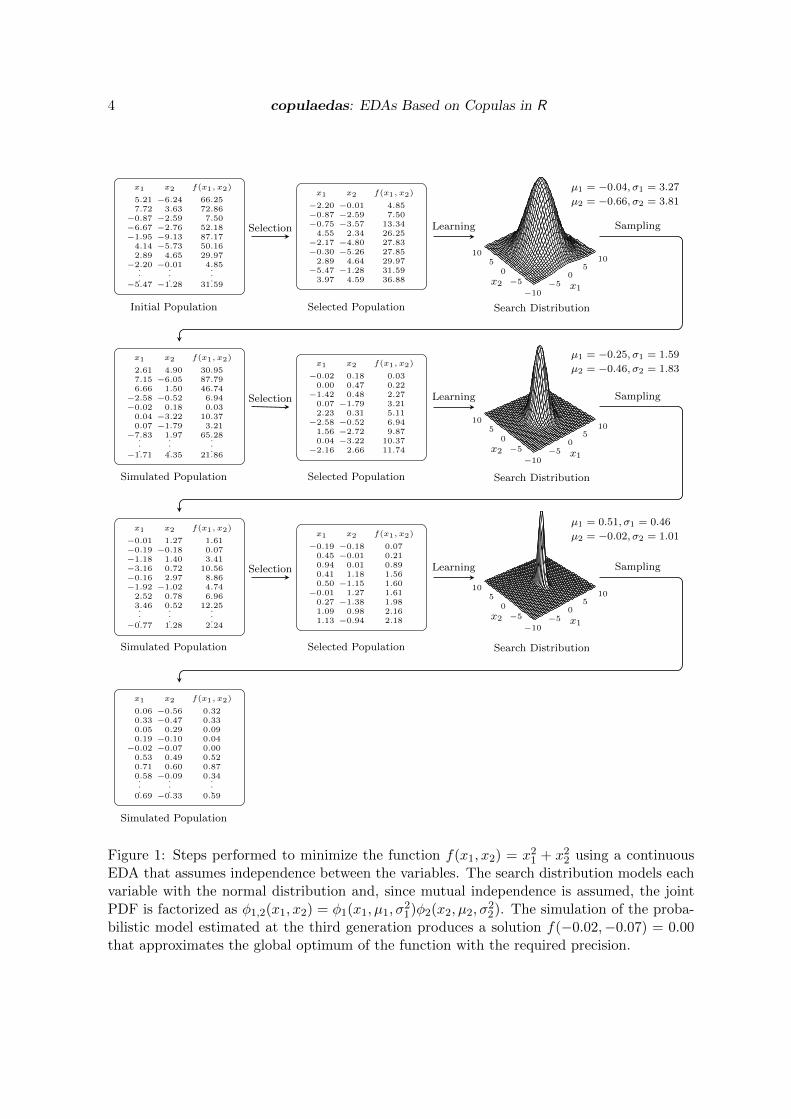
Let us illustrate the basic EDA procedure with a concrete example. Figure 1 shows thesteps performed to minimize the two-dimensional objective function f(x1, x2) = x21 + x22

http://CRAN.R-project.org/package=copulaedas


x1 x2 f(x1, x2)

5.21 −6.24 66.257.72 3.63 72.86

−0.87 −2.59 7.50−6.67 −2.76 52.18−1.95 −9.13 87.174.14 −5.73 50.162.89 4.65 29.97

−2.20 −0.01 4.85...

.

.

.

.

.

.−5.47 −1.28 31.59

x1 x2 f(x1, x2)

−2.20 −0.01 4.85−0.87 −2.59 7.50−0.75 −3.57 13.344.55 2.34 26.25

−2.17 −4.80 27.83−0.30 −5.26 27.852.89 4.64 29.97

−5.47 −1.28 31.593.97 4.59 36.88

−10−5

05

10

−5

05

10

x1x2

µ1 = −0.04, σ1 = 3.27

µ2 = −0.66, σ2 = 3.81

x1 x2 f(x1, x2)

2.61 4.90 30.957.15 −6.05 87.796.66 1.50 46.74

−2.58 −0.52 6.94−0.02 0.18 0.030.04 −3.22 10.370.07 −1.79 3.21

−7.83 1.97 65.28...

.

.

.

.

.

.−1.71 4.35 21.86

x1 x2 f(x1, x2)

−0.02 0.18 0.030.00 0.47 0.22

−1.42 0.48 2.270.07 −1.79 3.212.23 0.31 5.11

−2.58 −0.52 6.941.56 −2.72 9.870.04 −3.22 10.37

−2.16 2.66 11.74

−10−5

05

10

−5

05

10

x1x2

µ1 = −0.25, σ1 = 1.59

µ2 = −0.46, σ2 = 1.83

x1 x2 f(x1, x2)

−0.01 1.27 1.61−0.19 −0.18 0.07−1.18 1.40 3.41−3.16 0.72 10.56−0.16 2.97 8.86−1.92 −1.02 4.742.52 0.78 6.963.46 0.52 12.25...

.

.

.

.

.

.−0.77 1.28 2.24

x1 x2 f(x1, x2)

−0.19 −0.18 0.070.45 −0.01 0.210.94 0.01 0.890.41 1.18 1.560.50 −1.15 1.60

−0.01 1.27 1.610.27 −1.38 1.981.09 0.98 2.161.13 −0.94 2.18

−10−5

05

10

−5

05

10

x1x2

µ1 = 0.51, σ1 = 0.46

µ2 = −0.02, σ2 = 1.01

x1 x2 f(x1, x2)

0.06 −0.56 0.320.33 −0.47 0.330.05 0.29 0.090.19 −0.10 0.04

−0.02 −0.07 0.000.53 0.49 0.520.71 0.60 0.870.58 −0.09 0.34...

.

.

.

.

.

.0.69 −0.33 0.59

Initial Population

Simulated Population



Selected Population

Selected Population

Selected Population

Search Distribution

Search Distribution

Search Distribution

Selection Learning Sampling



Figure 1: Steps performed to minimize the function f(x1, x2) = x21 + x22 using a continuousEDA that assumes independence between the variables. The search distribution models eachvariable with the normal distribution and, since mutual independence is assumed, the jointPDF is factorized as φ1,2(x1, x2) = φ1(x1, µ1, σ

21)φ2(x2, µ2, σ

22). The simulation of the proba-

bilistic model estimated at the third generation produces a solution f(−0.02,−0.07) = 0.00that approximates the global optimum of the function with the required precision.


i← 1repeat

if i = 1 thenGenerate an initial population P1 using a seeding method.Evaluate the solutions in the population P1.If required, apply a local optimization method to the population P1.

elseSelect a population PSelectedi from Pi−1 according to a selection method.Learn a probabilistic model Mi from PSelectedi using a learning method.

Sample a new population PSampledi from Mi using a sampling method.

Evaluate the solutions in the population PSampledi .

If required, apply a local optimization method to the population PSampledi .

Create the population Pi from Pi−1 and PSampledi using a replacement method.end ifIf required, report progress information using a reporting method.i← i+ 1

until A criterion of the termination method is met.

Algorithm 1: Pseudocode of an EDA.

using a simple continuous EDA that assumes independence between the problem variables.Specifically, we aim to find the global optimum of the function f(0, 0) = 0 with a precision oftwo decimal places.

The algorithm starts by generating an initial population of 30 candidate solutions from acontinuous uniform distribution in [−10, 10]2. Out of this initial sampling, the best solutionfound so far is f(−2.20,−0.01) = 4.85. Next, the initial population is ranked accordingto their evaluation in f(x1, x2), and the best 30% of the solutions is selected to estimatethe probabilistic model. This EDA factorizes the joint probability density function (PDF)of the best solutions as φ1,2(x1, x2) = φ1(x1, µ1, σ

21)φ2(x2, µ2, σ

22), which describes mutual

independence, and where φ1 denotes the univariate normal PDF of x1 with mean µ1 andvariance σ21, and φ1 denotes the univariate normal PDF of x2 with mean µ1 and variance σ22.In the first generation, the parameters of the probabilistic model are µ1 = −0.04, σ1 = 3.27,µ2 = −0.66 and σ2 = 3.81. The second generation starts with the simulation of a newpopulation from the estimated probabilistic model. Afterwards, the same selection procedureis repeated and the resulting selected population is used to learn a new probabilistic model.These steps are then repeated for a third generation.

Notice how in the first three generations the refinement of the probabilistic model that repre-sents the best solutions is evidenced in the reduction of the variance of the marginal distribu-tions towards a mean value around zero. Also, the convergence of the algorithm is reflectedin the reduction of the value of the objective function from one generation to another. Ulti-mately, the simulation of the probabilistic model estimated at the third generation producesf(−0.02,−0.07) = 0.00, which satisfies our requirements and the algorithm terminates.

In practice, EDAs include other steps in addition to the ones illustrated in the previousbasic example. The general procedure of an EDA implemented in copulaedas is outlined inAlgorithm 1. In the following, we provide a description of the purpose of the main steps of


the algorithm, which are highlighted in italics in the pseudocode:

� The first step is the generation of an initial population of solutions following a seedingmethod, which is usually random, but it can use a particular heuristic when a prioriinformation about the characteristics of the problem is available.

� The results of global optimization algorithms such as EDAs can often be improved ifcombined with local optimization methods that look for better solutions in the neigh-borhood of each candidate solution. Local optimization methods can also be used toimplement repairing methods for constrained problems where the simulated solutionsmay be unfeasible and a strategy to repair these solutions is available.

� A selection method is used to determine the most promising solutions of the popula-tion. An example selection method is truncation selection, which creates the selectedpopulation with a percentage of the best solutions of the current population.

� The estimation and simulation of the search distribution are the essential steps of anEDA. These steps are implemented by learning and sampling methods, which are tightlyrelated. Learning methods estimate the structure and parameters of the probabilisticmodel used by the algorithm from the selected population, while sampling methods areused to generate new solutions from the estimated probabilistic model.

� A replacement method is used to incorporate a new group of solutions into the currentpopulation. For example, a replacement strategy is to substitute the current popula-tion with the newly sampled population. Other replacement strategies retain the bestsolutions found so far or try to maintain the diversity of solutions.

� Reporting methods provide progress information during the execution of the EDA. Rel-evant progress information can be the number of evaluations of the objective functionand the best solution found so far.

� A termination method determines when the algorithm stops according to certain criteria;for example, when a fixed number of function evaluations are realized or a certain valueof the objective function is reached.

Although it was possible to locate with the required precision the optimum of the simplefunction presented in this section, it is not always possible to perform a successful search byconsidering only the marginal information. As we show later in this paper, the assumptionof independence between the variables constitutes a strong limitation that may compromisethe convergence of an EDA. The use of information about the relationships between thevariables allows searching efficiently for the best solutions and it constitutes one of the mainadvantages of EDAs. Among the algorithms that consider dependences between the variables,we are particularly interested in EDAs whose learning and sampling steps involve probabilisticmodels based on copulas. The next section provides an overview of such algorithms.

2.2. Overview of EDAs based on copulas

To the best of our knowledge, the technical report (Soto, Ochoa, and Arderı 2007) and thetheses (Arderı 2007; Barba-Moreno 2007) constitute the first attempts to incorporate copulas


into EDAs. Since then, a considerable number of EDAs based on copula theory have beenproposed in the literature and, as evidence of its increasing popularity, the use of copulas inEDAs has been identified as an emerging approach for the solution of real-valued optimizationproblems (Hauschild and Pelikan 2011).

The learning step of copula-based EDAs consists of two tasks: the estimation of the marginaldistributions and the estimation of the probabilistic dependence structure. In general, thesetasks have been performed by following one of the two-step estimation procedures known inthe copula literature as the IFM (inference functions for margins; Joe and Xu 1996; Joe 2005)and the semiparametric estimation method (Genest, Ghoudi, and Rivest 1995). Firstly, themarginal distributions are estimated and the selected population is transformed into uniformlydistributed variables in (0, 1) by means of the evaluation of each marginal cumulative distri-bution function. Secondly, the transformed population is used to estimate a copula-basedmodel of the dependence structure among the variables. Usually, a particular parametric dis-tribution (e.g., normal or beta) is assumed for each margin and its parameters are estimatedby maximum likelihood (see e.g., Soto et al. 2007; Salinas-Gutierrez, Hernandez-Aguirre, andVilla-Diharce 2009). In other cases, empirical marginal distributions or kernel density estima-tion have been used (see e.g., Soto et al. 2007; Gao 2009; Cuesta-Infante, Santana, Hidalgo,Bielza, and naga 2010). The simulation step typically starts with the generation of a popu-lation of uniformly distributed variables in (0, 1) with the dependence structure described bythe copula-based model that was estimated in the learning step. Finally, this uniform popu-lation is transformed to the domain of the variables through the evaluation of the inverse ofeach marginal cumulative distribution function.

According to the copula model being used, EDAs based on copulas can be classified as EDAsbased on either multivariate or factorized copulas. In the rest of this section we give an overalldescription of representative algorithms belonging to each group that have been proposed inthe literature.

EDAs based on multivariate copulas

The research on EDAs based on multivariate copulas has focused on the use of multivariateelliptical copulas (Abdous, Genest, and Remillard 2005; Fang, Fang, and Kotz 2002) andArchimedean copulas (Joe 1997; McNeil and Neslehova 2009). The algorithms described inSoto et al. (2007); Arderı (2007) and Barba-Moreno (2007) are both based on the multivariatenormal copula and theoretically similar, but they present differences in the estimation of themarginal distributions and the use of techniques such as variance scaling. Wang, Zeng, andHong (2009b) present an EDA based on the bivariate normal copula and, since only normalmarginal distributions are used, the proposed algorithm is equivalent to EMNA (estimation ofmultivariate normal algorithm; Larranaga, Lozano, and Bengoetxea 2001). On the other hand,the algorithms presented in Wang, Zeng, and Hong (2009a) and Gao (2009) use exchangeableArchimedean copulas. Wang et al. (2009a) propose two algorithms that use Clayton and Ali-Mikhail-Haq copulas with fixed parameters, while Gao (2009) does not state which particularmembers of the family of Archimedean copulas are used.

Two EDAs based on multivariate copulas are implemented in copulaedas, one is based onthe product or independence copula and the other on the normal copula. The first algorithmis UMDA (univariate marginal distribution algorithm) for continuous variables (Larranaga,Etxeberria, Lozano, and Pena 1999, 2000), which can be integrated into the framework of


copula-based EDAs although originally it was not defined in terms of copulas. A consequenceof Sklar’s Theorem is that random variables are independent if and only if the underlyingcopula is the product copula. Thus, UMDA can be described as an EDA that models thedependence structure between the variables using a multivariate product copula.

The second EDA based on a multivariate copula implemented in copulaedas is GCEDA (Gaus-sian copula estimation of distribution algorithm; Soto et al. 2007; Arderı 2007). This algorithmis based on the multivariate normal copula, which allows the construction of multivariatedistributions with normal dependence structure and non-normal margins. The dependencestructure of the multivariate normal copula is determined by a positive-definite correlationmatrix. If the marginal distributions are not normal, the correlation matrix is estimatedthrough the inversion of the non-parametric estimator of Kendall’s tau for each pair of vari-ables (see e.g., Genest and Favre 2007; Hult and Lindskog 2002). If the resulting matrix isnot positive-definite, the transformation proposed by Rousseeuw and Molenberghs (1993) isapplied. GCEDA is equivalent to EMNA when all the marginal distributions are normal.

EDAs based on copula factorizations

The use of multivariate copulas to model the dependence structure between the variables offersa considerable number of advantages over the use of the multivariate normal distribution;nevertheless, it presents limitations. The number of tractable copulas available when morethan two variables are involved is limited, most available copulas are just investigated in thebivariate case. In addition, the multivariate elliptical copulas might not be appropriate whenall pairs of variables do not have the same dependence structure. Another limitation is thatsome multivariate extensions, such as exchangeable Archimedean copulas or the multivariatet copula, have only one parameter to describe certain aspects of the overall dependence. Thischaracteristic can be a serious limitation when the type and strength of the dependence isnot the same for all pairs of variables. One alternative to these limitations is to use copulafactorizations that build high-dimensional probabilistic models by using lower-dimensionalcopulas as building blocks. Several EDAs based on copula factorizations, such as nestedArchimedean copulas (Joe 1997) and vines (Joe 1996; Bedford and Cooke 2001; Aas et al.2009), have been proposed in the literature.

The EDA introduced in Salinas-Gutierrez et al. (2009) is an extension of MIMIC (mutualinformation maximization for input clustering) for continuous domains (Larranaga et al. 1999,2000) that uses bivariate copulas in a chain structure instead of bivariate normal distributions.Two instances of this algorithm were presented, one uses normal copulas and the other Frankcopulas. In Section 4.2, we illustrate the implementation of this algorithm using copulaedas.

The exchangeable Archimedean copulas employed in Wang et al. (2009a) and Gao (2009)represent highly specialized dependence structures (Berg and Aas 2007; McNeil 2008). Withinthe domain of Archimedean copulas, nested Archimedean copulas provide a more flexiblealternative to build multivariate copula distributions. In particular, hierarchically nestedArchimedean copulas present one of the most flexible solutions among the different nestingstructures that have been studied (see e.g., Berg and Aas 2007 for a review). Building fromthese models, Ye, Gao, Wang, and Zeng (2010) propose an EDA that uses a representationof hierarchically nested Archimedean copulas based on Levy subordinators (Hering, Hofert,Mai, and Scherer 2010).

Cuesta-Infante et al. (2010) investigate the use of bivariate empirical copulas and a multi-


variate extension of Archimedean copulas. The EDA based on bivariate empirical copulasis completely nonparametric: it employs empirical marginal distributions and a constructionbased on bivariate empirical copulas to represent the dependence between the variables. Themarginal distributions and the bivariate empirical copulas are defined through the linear in-terpolation of the sample in the selected population. The EDA based on Archimedean copulasuses a construction similar to a fully nested Archimedean copula and uses copulas from one ofthe families Frank, Clayton or HRT (i.e., heavy right tail copula or Clayton survival copula).The parameters of the copulas are fixed to a constant value, i.e., not estimated from the se-lected population. The marginal distributions are modeled as in the EDA based on bivariateempirical copulas.

The class of VEDAs (vine EDAs) is introduced in Soto and Gonzalez-Fernandez (2010) andGonzalez-Fernandez (2011). Algorithms of this class model the search distributions usingregular vines, which are graphical models that represent a multivariate distribution by de-composing the corresponding multivariate density into conditional bivariate copulas, uncon-ditional bivariate copulas and univariate densities. In particular, VEDAs are based on thesimplified pair-copula construction (Haff, Aas, and Frigessi 2010), which assumes that thebivariate copulas depend on the conditioning variables only through their arguments. Sinceall bivariate copulas do not have to belong to the same family, regular vines model a richvariety of dependences by combining bivariate copulas from different families.

A regular vine on n variables is a set of nested trees T1, . . . , Tn−1, where the edges of tree Tjare the nodes of the tree Tj+1 with j = 1, . . . , n − 2. The edges of the trees representthe bivariate copulas in the decomposition and the nodes their arguments. Moreover, theproximity condition requires that two nodes in tree Tj+1 are joined by an edge only if thecorresponding edges in Tj share a common node. C-vines (canonical vines) and D-vines(drawable vines) are two particular types of regular vines, each of which determines a specificdecomposition of the multivariate density. In a C-vine, each tree Tj has a unique root nodethat is connected to n− j edges. In a D-vine, no node is connected to more than two edges.Two EDAs based on regular vines are presented in Soto and Gonzalez-Fernandez (2010) andGonzalez-Fernandez (2011): CVEDA (C-vine EDA) and DVEDA (D-vine EDA) based onC-vines and D-vines, respectively. Since both algorithms are implemented in copulaedas, wedescribe them in more detail in the rest of this section.

The general idea of the simulation and inference methods for C-vines and D-vines was devel-oped by Aas et al. (2009). The simulation algorithm is based on the conditional distributionmethod (see e.g., Devroye 1986), while the inference method should consider two main aspects:the selection of the structure of the vines and the choice of the bivariate copulas. In the restof this section we describe how these aspects are performed in the particular implementationof CVEDA and DVEDA.

The selection of the structure of C-vines and D-vines is restricted to the selection of thebivariate dependences explicitly modeled in the first tree. This is accomplished by usinggreedy heuristics, which use the empirical Kendall’s tau assigned to the edges of the tree. Ina C-vine, the node that maximizes the sum of the weights of its edges to the other nodes ischosen as the root of the first tree and a canonical root node is assumed for the rest of thetrees. In a D-vine, the construction of the first tree consists of finding the maximum weightedsequence of the variables, which can be transformed into a TSP (traveling salesman problem)instance (Brechmann 2010). For efficiency reasons, in copulaedas we find an approximatesolution of the TSP by using the cheapest insertion heuristic (Rosenkrantz, Stearns, and


Lewis, II 1977).

The selection of each bivariate copula in both CVEDA and DVEDA starts with an indepen-dence test (Genest and Remillard 2004; Genest, Quessy, and Remillard 2007). The productcopula is selected when there is not enough evidence against the null hypothesis of indepen-dence at a given significance level. Otherwise, the parameters of a group of candidate copulasare estimated and the copula that minimizes a Cramer-von Mises statistic of the empiricalcopula is selected (Genest and Remillard 2008).

The cost of the construction of C-vines and D-vines increases with the number of variables. Toreduce this cost, we apply the truncation strategy presented in Brechmann (2010), for whichthe theoretical justification can be found in Joe, Li, and Nikoloulopoulos (2010). When a vineis truncated at a certain tree during the tree-wise estimation procedure, all the copulas inthe subsequent trees are assumed to be product copulas. A model selection procedure basedon either AIC (Akaike information criterion; Akaike 1974) or BIC (Bayesian informationcriterion; Schwarz 1978) is applied to detect the required number of trees. This procedureexpands the tree Tj+1 if the value of the information criterion calculated up to the tree Tj+1

is smaller than the value obtained up to the previous tree; otherwise, the vine is truncatedat the tree Tj . At this point, it is important to note that the algorithm presented in Salinas-Gutierrez, Hernandez-Aguirre, and Villa-Diharce (2010) also uses a D-vine. In this algorithmonly normal copulas are fitted in the first two trees and conditional independence is assumedin the rest of the trees, i.e., the D-vine is always truncated at the second tree.

The implementation of CVEDA and DVEDA included in copulaedas uses by default thetruncation procedure based on AIC and the candidate copulas normal, t, Clayton, Frank andGumbel. The parameters of all copulas but the t copula are estimated using the method ofmoments. For the t copula, the correlation coefficient is computed as in the normal copula, andthe degrees of freedom are estimated by maximum likelihood with the correlation parameterfixed (Demarta and McNeil 2005).

3. Implementation in R

According to the review presented by Santana (2011), the approach followed for the imple-mentation of EDA software currently available through the Internet can be classified intothree categories: (1) implementation of a single EDA, (2) independent implementation ofmultiple EDAs, and (3) common modular implementation of multiple EDAs. In our opin-ion, the third approach offers greater flexibility for the EDA community. In these modularimplementations, the EDA components (e.g., learning and sampling methods) are indepen-dently programmed by taking advantage of the common schema shared by most EDAs. Thismodularity allows the creation and validation of new EDA proposals that combine differentcomponents, and promotes code factorization. Additionally, as the EDAs are grouped underthe same framework, it facilitates performing empirical studies to compare the behavior ofdifferent algorithms. Existing members of this class are ParadisEO (Cahon, Melab, and Talbi2004; DOLPHIN Project Team 2012), LiO (Mateo and de la Ossa 2006, 2007), Mateda-2.0(Santana et al. 2009, 2010) and now copulaedas.

The implementation of copulaedas follows an object-oriented design inspired by the Mateda-2.0 toolbox for MATLAB (The MathWorks, Inc. 2014). EDAs implemented in the packageare represented by S4 classes (Chambers 2008) with generic functions for their main steps.


Generic function Description

edaSeed Seeding method. The default method edaSeedUniform generates thevalues of each variable in the initial population from a continuous uni-form distribution.

edaOptimize Local optimization method. The use of a local optimization method isdisabled by default.

edaSelect Selection method. The default method edaSelectTruncation imple-ments truncation selection.

edaLearn Learning method. No default method.edaSample Sampling method. No default method.edaReplace Replacement method. The default method edaReplaceComplete

completely replaces the current population with the new population.edaReport Reporting method. Reporting progress information is disabled by

default.edaTerminate Termination method. The default method edaTerminateMaxGen ends

the execution of the algorithm after a maximum number of generations.

Table 1: Description of the generic functions that implement the steps of the general procedureof an EDA outlined in Algorithm 1 and their default methods.

The base class of EDAs in the package is ‘EDA’, which has two slots: name and parameters.The name slot stores a character string with the name of the EDA and it is used by theshow method to print the name of the algorithm when it is called with an ‘EDA’ instance asargument. The parameters slot stores all the EDA parameters in a list.

In copulaedas, each step of the general procedure of an EDA outlined in Algorithm 1 is repre-sented by a generic function that expects an ‘EDA’ instance as its first argument. Table 1 showsa description of these functions and their default methods. The help page of these genericfunctions in the documentation of copulaedas contains information about their arguments,return value, and methods already implemented in the package.

The generic functions and their methods that implement the steps of an EDA look at theparameters slot of the ‘EDA’ instance received as first argument for the values of the parame-ters that affect their behavior. Only named members of the list must be used and reasonabledefault values should be assumed when a certain component is missing. The help page ofeach generic function describes the members of the list in the parameters slot interpreted byeach function and their default values.

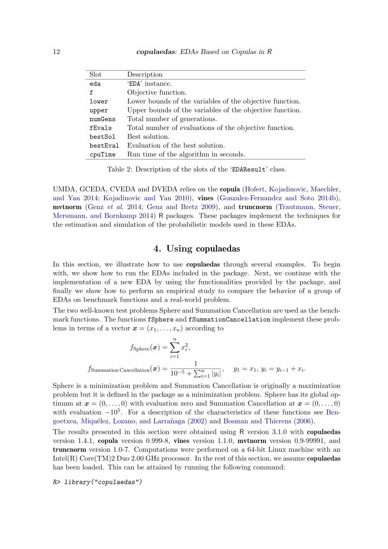
The edaRun function implements the Algorithm 1 by linking together the generic functions foreach step. This function expects four arguments: the ‘EDA’ instance, the objective functionand two vectors specifying the lower and upper bounds of the variables of the objectivefunction. The length of the vectors with the lower and upper bounds should be the same,since it determines the number of variables of the objective function. When edaRun is called,it runs the main loop of the EDA until the call to the edaTerminate generic function returnsTRUE. Then, the function returns an instance of the ‘EDAResult’ class that encapsulates theresults of the algorithm. A description of the slots of this class is given in Table 2.

Two subclasses of ‘EDA’ are already defined in copulaedas: ‘CEDA’, that represents EDAs basedon multivariate copulas; and ‘VEDA’, that represents vine-based EDAs. The implementation of


Slot Description

eda ‘EDA’ instance.f Objective function.lower Lower bounds of the variables of the objective function.upper Upper bounds of the variables of the objective function.numGens Total number of generations.fEvals Total number of evaluations of the objective function.bestSol Best solution.bestEval Evaluation of the best solution.cpuTime Run time of the algorithm in seconds.

Table 2: Description of the slots of the ‘EDAResult’ class.

UMDA, GCEDA, CVEDA and DVEDA relies on the copula (Hofert, Kojadinovic, Maechler,and Yan 2014; Kojadinovic and Yan 2010), vines (Gonzalez-Fernandez and Soto 2014b),mvtnorm (Genz et al. 2014; Genz and Bretz 2009), and truncnorm (Trautmann, Steuer,Mersmann, and Bornkamp 2014) R packages. These packages implement the techniques forthe estimation and simulation of the probabilistic models used in these EDAs.

4. Using copulaedas

In this section, we illustrate how to use copulaedas through several examples. To beginwith, we show how to run the EDAs included in the package. Next, we continue with theimplementation of a new EDA by using the functionalities provided by the package, andfinally we show how to perform an empirical study to compare the behavior of a group ofEDAs on benchmark functions and a real-world problem.

The two well-known test problems Sphere and Summation Cancellation are used as the bench-mark functions. The functions fSphere and fSummationCancellation implement these prob-lems in terms of a vector x = (x1, . . . , xn) according to

fSphere(x) =n∑i=1

x2i ,

fSummationCancellation(x) =1

10−5 +∑n

i=1 |yi|, y1 = x1, yi = yi−1 + xi.

Sphere is a minimization problem and Summation Cancellation is originally a maximizationproblem but it is defined in the package as a minimization problem. Sphere has its global op-timum at x = (0, . . . , 0) with evaluation zero and Summation Cancellation at x = (0, . . . , 0)with evaluation −105. For a description of the characteristics of these functions see Ben-goetxea, Miquelez, Lozano, and Larranaga (2002) and Bosman and Thierens (2006).

The results presented in this section were obtained using R version 3.1.0 with copulaedasversion 1.4.1, copula version 0.999-8, vines version 1.1.0, mvtnorm version 0.9-99991, andtruncnorm version 1.0-7. Computations were performed on a 64-bit Linux machine with anIntel(R) Core(TM)2 Duo 2.00 GHz processor. In the rest of this section, we assume copulaedashas been loaded. This can be attained by running the following command:

R> library("copulaedas")


4.1. Running the EDAs included in the package

We begin by illustrating how to run the EDAs based on copulas implemented in copulaedas.As an example, we execute GCEDA to optimize Sphere in five dimensions. Before creating anew instance of the ‘CEDA’ class for EDAs based on multivariate copulas, we set up the genericfunctions for the steps of the EDA according to the expected behavior of GCEDA. The termi-nation criterion is either to find the optimum of the objective function or to reach a maximumnumber of generations. That is why we set the method for the edaTerminate generic functionto a combination of the functions edaTerminateEval and edaTerminateMaxGen through theauxiliary function edaTerminateCombined.

R> setMethod("edaTerminate", "EDA",

+ edaTerminateCombined(edaTerminateEval, edaTerminateMaxGen))

The method for the edaReport generic function is set to edaReportSimple to make thealgorithm print progress information at each generation. This function prints one line at eachiteration of the EDA with the minimum, mean and standard deviation of the evaluation ofthe solutions in the current population.

R> setMethod("edaReport", "EDA", edaReportSimple)

Note that these methods were set for the base class ‘EDA’ and therefore they will be inheritedby all subclasses. Generally, we find it convenient to define methods of the generic functionsthat implement the steps of the EDA for the base class, except when different subclassesshould use different methods.

The auxiliary function ‘CEDA’ can be used to create instances of the class with the samename. All the arguments of the function are interpreted as parameters of the EDA to beadded as members of the list in the parameters slot of the new instance. An instanceof ‘CEDA’ corresponding to GCEDA using empirical marginal distributions smoothed withnormal kernels can be created as follows:

R> gceda <- CEDA(copula = "normal", margin = "kernel", popSize = 200,

+ fEval = 0, fEvalTol = 1e-6, maxGen = 50)

R> gceda@name <- "Gaussian Copula Estimation of Distribution Algorithm"

The methods that implement the generic functions edaLearn and edaSample for ‘CEDA’ in-stances expect three parameters. The copula parameter specifies the multivariate copulaand it should be set to "normal" for GCEDA. The marginal distributions are determinedby the value of margin and all EDAs implemented in the package use this parameter for thesame purpose. As margin is set to "kernel", the algorithm will look for three functionsnamed fkernel, pkernel and qkernel already defined in the package to fit the parametersof the margins and to evaluate the distribution and quantile functions, respectively. Thefkernel function computes the bandwidth parameter of the normal kernel according to therule-of-thumb of Silverman (1986) and pkernel implements the empirical cumulative dis-tribution function. The quantile function is evaluated following the procedure described inAzzalini (1981). The popSize parameter determines the population size while the rest of thearguments of CEDA are parameters of the functions that implement the termination criterion.


Now, we can run GCEDA by calling edaRun. The lower and upper bounds of the variablesare set so that the values of the variables in the optimum of the function are located at 25%of the interval. It was shown in Arderı (2007) and Soto et al. (2014) that the use of empiricalmarginal distributions smoothed with normal kernels improves the behavior of GCEDA whenthe initial population is generated asymmetrically with respect to the optimum of the function.

R> set.seed(12345)

R> result <- edaRun(gceda, fSphere, rep(-300, 5), rep(900, 5))

Generation Minimum Mean Std. Dev.

1 1.522570e+05 1.083606e+06 5.341601e+05

2 2.175992e+04 5.612769e+05 3.307403e+05

3 8.728486e+03 2.492247e+05 1.496334e+05

4 4.536507e+03 1.025119e+05 5.829982e+04

5 5.827775e+03 5.126260e+04 2.983622e+04

6 2.402107e+03 2.527349e+04 1.430142e+04

7 9.170485e+02 1.312806e+04 6.815822e+03

8 4.591915e+02 6.726731e+03 4.150888e+03

9 2.448265e+02 3.308515e+03 1.947486e+03

10 7.727107e+01 1.488859e+03 8.567864e+02

11 4.601731e+01 6.030030e+02 3.529036e+02

12 8.555769e+00 2.381415e+02 1.568382e+02

13 1.865639e+00 1.000919e+02 6.078611e+01

14 5.157326e+00 4.404530e+01 2.413589e+01

15 1.788793e+00 2.195864e+01 1.136284e+01

16 7.418832e-01 1.113184e+01 6.157461e+00

17 6.223596e-01 4.880880e+00 2.723950e+00

18 4.520045e-02 2.327805e+00 1.287697e+00

19 6.981399e-02 1.123582e+00 6.956201e-01

20 3.440069e-02 5.118243e-01 2.985175e-01

21 1.370064e-02 1.960786e-01 1.329600e-01

22 3.050774e-03 7.634156e-02 4.453917e-02

23 1.367716e-03 3.400907e-02 2.056747e-02

24 7.599946e-04 1.461478e-02 8.861180e-03

25 4.009605e-04 6.488932e-03 4.043431e-03

26 1.083879e-04 2.625759e-03 1.618058e-03

27 8.441887e-05 1.079075e-03 5.759307e-04

28 3.429462e-05 5.077934e-04 3.055568e-04

29 1.999004e-05 2.232605e-04 1.198675e-04

30 1.038719e-05 1.104123e-04 5.888948e-05

31 6.297005e-06 5.516721e-05 2.945027e-05

32 1.034002e-06 2.537823e-05 1.295004e-05

33 8.483830e-07 1.332463e-05 7.399488e-06

The result variable contains an instance of the ‘EDAResult’ class. The show method printsthe results of the execution of the algorithm.

R> show(result)


Results for Gaussian Copula Estimation of Distribution Algorithm

Best function evaluation 8.48383e-07

No. of generations 33

No. of function evaluations 6600

CPU time 7.895 seconds

Due to the stochastic nature of EDAs, it is often useful to analyze a sequence of independentruns to ensure reliable results. The edaIndepRuns function supports performing this task.To avoid generating lot of unnecessary output, we first disable reporting progress informationon each generation by setting edaReport to edaReportDisabled and then we invoke theedaIndepRuns function to perform 30 independent runs of GCEDA.

R> setMethod("edaReport", "EDA", edaReportDisabled)

R> set.seed(12345)

R> results <- edaIndepRuns(gceda, fSphere, rep(-300, 5), rep(900, 5), 30)

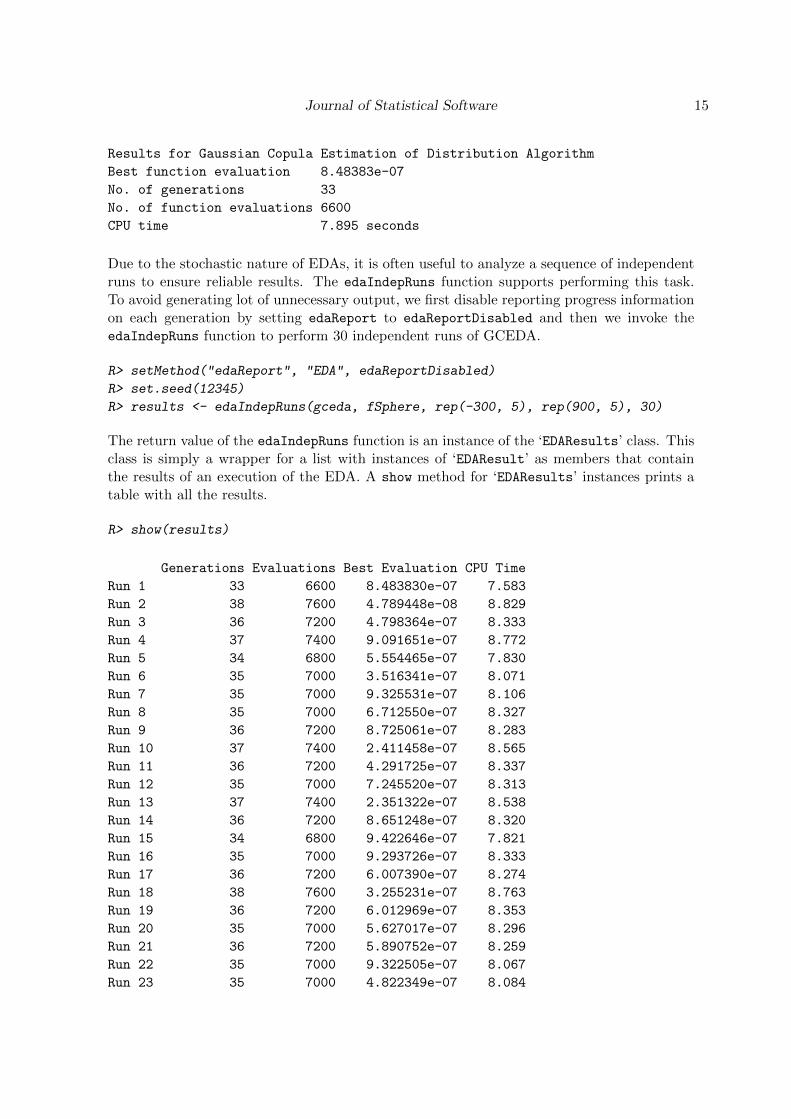
The return value of the edaIndepRuns function is an instance of the ‘EDAResults’ class. Thisclass is simply a wrapper for a list with instances of ‘EDAResult’ as members that containthe results of an execution of the EDA. A show method for ‘EDAResults’ instances prints atable with all the results.

R> show(results)

Generations Evaluations Best Evaluation CPU Time

Run 1 33 6600 8.483830e-07 7.583

Run 2 38 7600 4.789448e-08 8.829

Run 3 36 7200 4.798364e-07 8.333

Run 4 37 7400 9.091651e-07 8.772

Run 5 34 6800 5.554465e-07 7.830

Run 6 35 7000 3.516341e-07 8.071

Run 7 35 7000 9.325531e-07 8.106

Run 8 35 7000 6.712550e-07 8.327

Run 9 36 7200 8.725061e-07 8.283

Run 10 37 7400 2.411458e-07 8.565

Run 11 36 7200 4.291725e-07 8.337

Run 12 35 7000 7.245520e-07 8.313

Run 13 37 7400 2.351322e-07 8.538

Run 14 36 7200 8.651248e-07 8.320

Run 15 34 6800 9.422646e-07 7.821

Run 16 35 7000 9.293726e-07 8.333

Run 17 36 7200 6.007390e-07 8.274

Run 18 38 7600 3.255231e-07 8.763

Run 19 36 7200 6.012969e-07 8.353

Run 20 35 7000 5.627017e-07 8.296

Run 21 36 7200 5.890752e-07 8.259

Run 22 35 7000 9.322505e-07 8.067

Run 23 35 7000 4.822349e-07 8.084


Run 24 34 6800 7.895408e-07 7.924

Run 25 36 7200 6.970180e-07 8.519

Run 26 34 6800 3.990247e-07 7.808

Run 27 35 7000 8.876874e-07 8.055

Run 28 33 6600 8.646387e-07 7.622

Run 29 36 7200 9.072113e-07 8.519

Run 30 35 7000 9.414666e-07 8.040

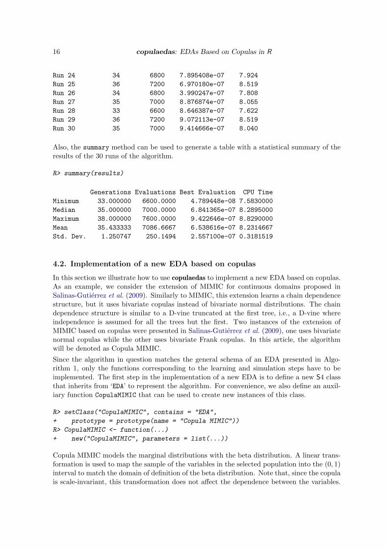
Also, the summary method can be used to generate a table with a statistical summary of theresults of the 30 runs of the algorithm.

R> summary(results)


Minimum 33.000000 6600.0000 4.789448e-08 7.5830000

Median 35.000000 7000.0000 6.841365e-07 8.2895000

Maximum 38.000000 7600.0000 9.422646e-07 8.8290000

Mean 35.433333 7086.6667 6.538616e-07 8.2314667

Std. Dev. 1.250747 250.1494 2.557100e-07 0.3181519

4.2. Implementation of a new EDA based on copulas

In this section we illustrate how to use copulaedas to implement a new EDA based on copulas.As an example, we consider the extension of MIMIC for continuous domains proposed inSalinas-Gutierrez et al. (2009). Similarly to MIMIC, this extension learns a chain dependencestructure, but it uses bivariate copulas instead of bivariate normal distributions. The chaindependence structure is similar to a D-vine truncated at the first tree, i.e., a D-vine whereindependence is assumed for all the trees but the first. Two instances of the extension ofMIMIC based on copulas were presented in Salinas-Gutierrez et al. (2009), one uses bivariatenormal copulas while the other uses bivariate Frank copulas. In this article, the algorithmwill be denoted as Copula MIMIC.

Since the algorithm in question matches the general schema of an EDA presented in Algo-rithm 1, only the functions corresponding to the learning and simulation steps have to beimplemented. The first step in the implementation of a new EDA is to define a new S4 classthat inherits from ‘EDA’ to represent the algorithm. For convenience, we also define an auxil-iary function CopulaMIMIC that can be used to create new instances of this class.

R> setClass("CopulaMIMIC", contains = "EDA",

+ prototype = prototype(name = "Copula MIMIC"))

R> CopulaMIMIC <- function(...)

+ new("CopulaMIMIC", parameters = list(...))

Copula MIMIC models the marginal distributions with the beta distribution. A linear trans-formation is used to map the sample of the variables in the selected population into the (0, 1)interval to match the domain of definition of the beta distribution. Note that, since the copulais scale-invariant, this transformation does not affect the dependence between the variables.


To be consistent with the margins already implemented in copulaedas, we define three func-tions with the common suffix betamargin and the prefixes f, p and q to fit the parametersof the margins and for the evaluation of the distribution and quantile functions, respectively.By following this convention, the algorithms already implemented in the package can use betamarginal distributions by setting the margin parameter to "betamargin".

R> fbetamargin <- function(x, lower, upper) {

+ x <- (x - lower) / (upper - lower)

+ loglik <- function(s) sum(dbeta(x, s[1], s[2], log = TRUE))

+ s <- optim(c(1, 1), loglik, control = list(fnscale = -1))$par

+ list(lower = lower, upper = upper, a = s[1], b = s[2])

+ }

R> pbetamargin <- function(q, lower, upper, a, b) {

+ q <- (q - lower) / (upper - lower)

+ pbeta(q, a, b)

+ }

R> qbetamargin <- function(p, lower, upper, a, b) {

+ q <- qbeta(p, a, b)

+ lower + q * (upper - lower)

+ }

The ‘CopulaMIMIC’ class inherits methods for the generic functions that implement all thesteps of the EDA except learning and sampling. To complete the implementation of thealgorithm, we must define the estimation and simulation of the probabilistic model as methodsfor the generic functions edaLearn and edaSample, respectively.

The method for edaLearn starts with the estimation of the parameters of the margins andthe transformation of the selected population to uniform variables in (0, 1). Then, the mutualinformation between all pairs of variables is calculated through the copula entropy (Davyand Doucet 2003). To accomplish this, the parameters of each possible bivariate copula areestimated by the method of maximum likelihood using the value obtained through the methodof moments as an initial approximation. To determine the chain dependence structure, apermutation of the variables that maximizes the pairwise mutual information must be selectedbut, since this is a computationally intensive task, a greedy algorithm is used to compute anapproximate solution (De Bonet, Isbell, and Viola 1997; Larranaga et al. 1999). Finally,the method for edaLearn returns a list with three components that represents the estimatedprobabilistic model: the parameters of the marginal distributions, the permutation of thevariables, and the copulas in the chain dependence structure.

R> edaLearnCopulaMIMIC <- function(eda, gen, previousModel,

+ selectedPop, selectedEval, lower, upper) {

+ margin <- eda@parameters$margin

+ copula <- eda@parameters$copula

+ if (is.null(margin)) margin <- "betamargin"

+ if (is.null(copula)) copula <- "normal"

+ fmargin <- get(paste("f", margin, sep = ""))

+ pmargin <- get(paste("p", margin, sep = ""))

+ copula <- switch(copula, normal = normalCopula(0),


+ frank = frankCopula(0))

+ n <- ncol(selectedPop)

+ # Estimate the parameters of the marginal distributions.

+ margins <- lapply(seq(length = n),

+ function(i) fmargin(selectedPop[, i], lower[i], upper[i]))

+ uniformPop <- sapply(seq(length = n), function(i) do.call(pmargin,

+ c(list(selectedPop[ , i]), margins[[i]])))

+ # Calculate pairwise mutual information by using copula entropy.

+ C <- matrix(list(NULL), nrow = n, ncol = n)

+ I <- matrix(0, nrow = n, ncol = n)

+ for (i in seq(from = 2, to = n)) {

+ for (j in seq(from = 1, to = i - 1)) {

+ # Estimate the parameters of the copula.

+ data <- cbind(uniformPop[, i], uniformPop[, j])

+ startCopula <- fitCopula(copula, data, method = "itau",

+ estimate.variance = FALSE)@copula

+ C[[i, j]] <- tryCatch(

+ fitCopula(startCopula, data, method = "ml",

+ start = startCopula@parameters,

+ estimate.variance = FALSE)@copula,

+ error = function(error) startCopula)

+ # Calculate mutual information.

+ if (is(C[[i, j]], "normalCopula")) {

+ I[i, j] <- -0.5 * log(1 - C[[i, j]]@parameters^2)

+ } else {

+ u <- rcopula(C[[i, j]], 100)

+ I[i, j] <- sum(log(dcopula(C[[i, j]], u))) / 100

+ }

+ C[[j, i]] <- C[[i, j]]

+ I[j, i] <- I[i, j]

+ }

+ }

+ # Select a permutation of the variables.

+ perm <- as.vector(arrayInd(which.max(I), dim(I)))

+ copulas <- C[perm[1], perm[2]]

+ I[perm, ] <- -Inf

+ for (k in seq(length = n - 2)) {

+ ik <- which.max(I[, perm[1]])

+ perm <- c(ik, perm)

+ copulas <- c(C[perm[1], perm[2]], copulas)

+ I[ik, ] <- -Inf

+ }

+ list(margins = margins, perm = perm, copulas = copulas)

+ }

R> setMethod("edaLearn", "CopulaMIMIC", edaLearnCopulaMIMIC)

The edaSample method receives the representation of the probabilistic model returned by


edaLearn as the model argument. The generation of a new solution with n variables startswith the simulation of an n-dimensional vector U having uniform marginal distributions in(0, 1) and the dependence described by the copulas in the chain dependence structure. Thefirst step is to simulate an independent uniform variable Uπn in (0, 1), where πn denotes thevariable in the position n of the permutation π selected by the edaLearn method. The rest ofthe uniform variables are simulated conditionally on the previously simulated variable by usingthe conditional copula C(Uπk |Uπk+1

), with k = n−1, n−2, . . . , 1. Finally, the new solution isdetermined through the evaluation of the beta quantile functions and the application of theinverse of the linear transformation.

R> edaSampleCopulaMIMIC <- function(eda, gen, model, lower, upper) {

+ popSize <- eda@parameters$popSize

+ margin <- eda@parameters$margin

+ if (is.null(popSize)) popSize <- 100

+ if (is.null(margin)) margin <- "betamargin"

+ qmargin <- get(paste("q", margin, sep = ""))

+ n <- length(model$margins)

+ perm <- model$perm

+ copulas <- model$copulas

+ # Simulate the chain structure with the copulas.

+ uniformPop <- matrix(0, nrow = popSize, ncol = n)

+ uniformPop[, perm[n]] <- runif(popSize)

+ for (k in seq(from = n - 1, to = 1)) {

+ u <- runif(popSize)

+ v <- uniformPop[, perm[k + 1]]

+ uniformPop[, perm[k]] <- hinverse(copulas[[k]], u, v)

+ }

+ # Evaluate the inverse of the marginal distributions.

+ pop <- sapply(seq(length = n), function(i) do.call(qmargin,

+ c(list(uniformPop[, i]), model$margins[[i]])))

+ pop

+ }

R> setMethod("edaSample", "CopulaMIMIC", edaSampleCopulaMIMIC)

The code fragments given above constitute the complete implementation of Copula MIMIC.As it was illustrated with GCEDA in the previous section, the algorithm can be executed bycreating an instance of the ‘CopulaMIMIC’ class and calling the edaRun function.

4.3. Performing an empirical study on benchmark problems

We now show how to use copulaedas to perform an empirical study of the behavior of agroup of EDAs based on copulas on benchmark problems. The algorithms to be comparedare UMDA, GCEDA, CVEDA, DVEDA and Copula MIMIC. The first four algorithms areincluded in copulaedas and the fifth algorithm was implemented in Section 4.2. The twofunctions Sphere and Summation Cancellation described at the beginning of Section 4 areconsidered as benchmark problems in 10 dimensions.

The aim of this empirical study is to assess the behavior of these algorithms when only linearand independence relationships are considered. Thus, only normal and product copulas are


used in these EDAs. UMDA and GCEDA use multivariate product and normal copulas,respectively. CVEDA and DVEDA are configured to combine bivariate product and normalcopulas in the vines. Copula MIMIC learns a chain dependence structure with normal copulas.All algorithms use normal marginal distributions. Note that in this case, GCEDA correspondsto EMNA and Copula MIMIC is similar to MIMIC for continuous domains. In the followingcode fragment, we create class instances corresponding to these algorithms.

R> umda <- CEDA(copula = "indep", margin = "norm")

R> umda@name <- "UMDA"

R> gceda <- CEDA(copula = "normal", margin = "norm")

R> gceda@name <- "GCEDA"

R> cveda <- VEDA(vine = "CVine", indepTestSigLevel = 0.01,

+ copulas = c("normal"), margin = "norm")

R> cveda@name <- "CVEDA"

R> dveda <- VEDA(vine = "DVine", indepTestSigLevel = 0.01,

+ copulas = c("normal"), margin = "norm")

R> dveda@name <- "DVEDA"

R> copulamimic <- CopulaMIMIC(copula = "normal", margin = "norm")

R> copulamimic@name <- "CopulaMIMIC"

The initial population is generated using the default edaSeed method, therefore, it is sampleduniformly in the real interval of each variable. The lower and upper bounds of the variables areset so that the values of the variables in the optimum of the function are located in the middleof the interval. We use the intervals [−600, 600] in Sphere and [−0.16, 0.16] in SummationCancellation. All algorithms use the default truncation selection method with a truncationfactor of 0.3. Three termination criteria are combined using the edaTerminateCombined

function: to find the global optimum of the function with a precision greater than 10−6, toreach 300000 function evaluations, or to loose diversity in the population (i.e., the standarddeviation of the evaluation of the solutions in the population is less than 10−8). Thesecriteria are implemented in the functions edaTerminateEval, edaTerminateMaxEvals andedaTerminateEvalStdDev, respectively.

The population size of EDAs along with the truncation method determine the sample availablefor the estimation of the search distribution. An arbitrary selection of the population sizecould lead to misleading conclusions of the results of the experiments. When the populationsize is too small, the search distributions might not be accurately estimated. On the otherhand, the use of an excessively large population size usually does not result in a better behaviorof the algorithms but certainly in a greater number of function evaluations. Therefore, weadvocate for the use of the critical population size when comparing the performance of EDAs.The critical population size is the minimum population size required by the algorithm to findthe global optimum of the function with a high success rate, e.g., to find the optimum in 30of 30 sequential independent runs.

An approximate value of the critical population size can be determined empirically using abisection method (see e.g., Pelikan 2005 for a pseudocode of the algorithm). The bisectionmethod begins with an initial interval where the critical population size should be locatedand discards one half of the interval at each step. This procedure is implemented in theedaCriticalPopSize function. In the experimental study carried out in this section, theinitial interval is set to [50, 2000]. If the critical population size is not found in this interval,


the results of the algorithm with the population size given by the upper bound are presented.

The complete empirical study consists of performing 30 independent runs of every algorithmon every function using the critical population size. We proceed with the definition of a listcontaining all algorithm-function pairs.

R> edas <- list(umda, gceda, cveda, dveda, copulamimic)

R> fNames <- c("Sphere", "SummationCancellation")

R> experiments <- list()

R> for (eda in edas) {

+ for (fName in fNames) {

+ experiment <- list(eda = eda, fName = fName)

+ experiments <- c(experiments, list(experiment))

+ }

+ }

Now we define a function to process the elements of the experiments list. This functionimplements all the experimental setup described before. The output of edaCriticalPopSizeand edaIndepRuns is redirected to a different plain text file for each algorithm-function pair.

R> runExperiment <- function(experiment) {

+ eda <- experiment$eda

+ fName <- experiment$fName

+ # Objective function parameters.

+ fInfo <- list(

+ Sphere = list(lower = -600, upper = 600, fEval = 0),

+ SummationCancellation = list(lower = -0.16, upper = 0.16,

+ fEval = -1e5))

+ lower <- rep(fInfo[[fName]]$lower, 10)

+ upper <- rep(fInfo[[fName]]$upper, 10)

+ f <- get(paste("f", fName, sep = ""))

+ # Configure termination criteria and disable reporting.

+ eda@parameters$fEval <- fInfo[[fName]]$fEval

+ eda@parameters$fEvalTol <- 1e-6

+ eda@parameters$fEvalStdDev <- 1e-8

+ eda@parameters$maxEvals <- 300000

+ setMethod("edaTerminate", "EDA",

+ edaTerminateCombined(edaTerminateEval, edaTerminateMaxEvals,

+ edaTerminateEvalStdDev))

+ setMethod("edaReport", "EDA", edaReportDisabled)

+ sink(paste(eda@name, "_", fName, ".txt", sep = ""))

+ # Determine the critical population size.

+ set.seed(12345)

+ results <- edaCriticalPopSize(eda, f, lower, upper,

+ eda@parameters$fEval, eda@parameters$fEvalTol, lowerPop = 50,

+ upperPop = 2000, totalRuns = 30, successRuns = 30,

+ stopPercent = 10, verbose = TRUE)

+ if (is.null(results)) {


Algorithm Success Pop. Evaluations Best Evaluation CPU Time

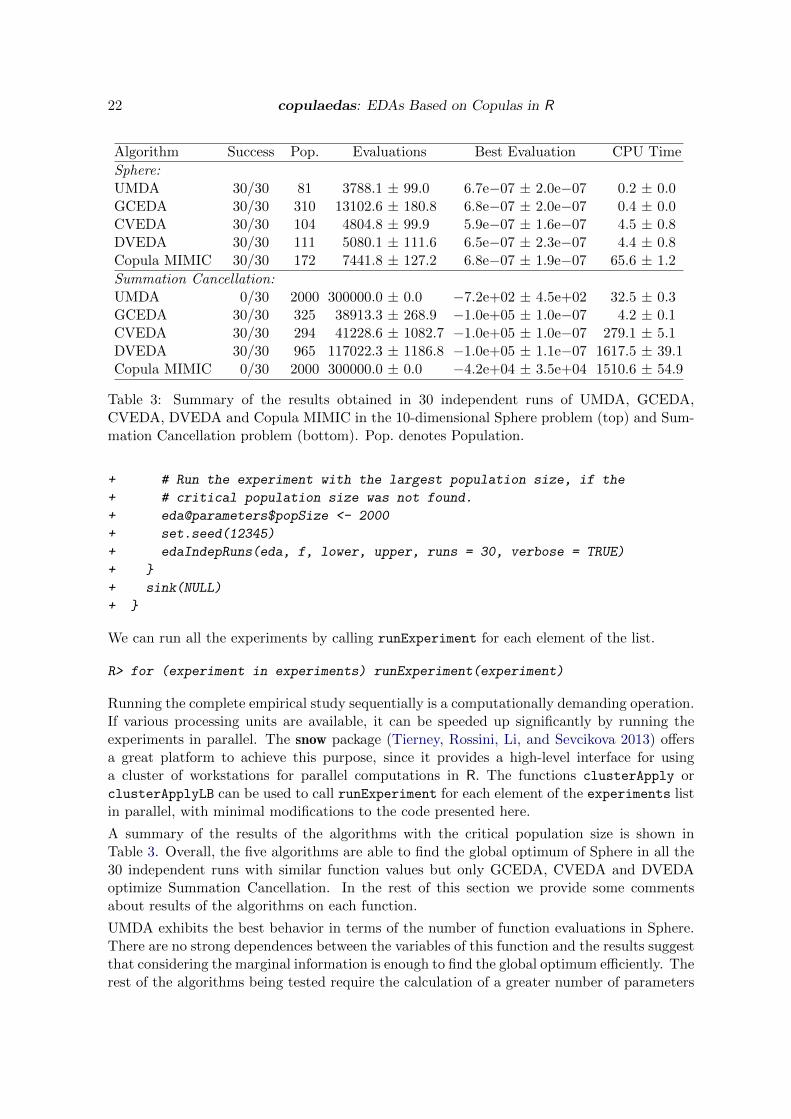
Sphere:UMDA 30/30 81 3788.1 ± 99.0 6.7e−07 ± 2.0e−07 0.2 ± 0.0GCEDA 30/30 310 13102.6 ± 180.8 6.8e−07 ± 2.0e−07 0.4 ± 0.0CVEDA 30/30 104 4804.8 ± 99.9 5.9e−07 ± 1.6e−07 4.5 ± 0.8DVEDA 30/30 111 5080.1 ± 111.6 6.5e−07 ± 2.3e−07 4.4 ± 0.8Copula MIMIC 30/30 172 7441.8 ± 127.2 6.8e−07 ± 1.9e−07 65.6 ± 1.2

Summation Cancellation:UMDA 0/30 2000 300000.0 ± 0.0 −7.2e+02 ± 4.5e+02 32.5 ± 0.3GCEDA 30/30 325 38913.3 ± 268.9 −1.0e+05 ± 1.0e−07 4.2 ± 0.1CVEDA 30/30 294 41228.6 ± 1082.7 −1.0e+05 ± 1.0e−07 279.1 ± 5.1DVEDA 30/30 965 117022.3 ± 1186.8 −1.0e+05 ± 1.1e−07 1617.5 ± 39.1Copula MIMIC 0/30 2000 300000.0 ± 0.0 −4.2e+04 ± 3.5e+04 1510.6 ± 54.9

Table 3: Summary of the results obtained in 30 independent runs of UMDA, GCEDA,CVEDA, DVEDA and Copula MIMIC in the 10-dimensional Sphere problem (top) and Sum-mation Cancellation problem (bottom). Pop. denotes Population.

+ # Run the experiment with the largest population size, if the

+ # critical population size was not found.

+ eda@parameters$popSize <- 2000

+ set.seed(12345)

+ edaIndepRuns(eda, f, lower, upper, runs = 30, verbose = TRUE)

+ }

+ sink(NULL)

+ }

We can run all the experiments by calling runExperiment for each element of the list.

R> for (experiment in experiments) runExperiment(experiment)

Running the complete empirical study sequentially is a computationally demanding operation.If various processing units are available, it can be speeded up significantly by running theexperiments in parallel. The snow package (Tierney, Rossini, Li, and Sevcikova 2013) offersa great platform to achieve this purpose, since it provides a high-level interface for usinga cluster of workstations for parallel computations in R. The functions clusterApply orclusterApplyLB can be used to call runExperiment for each element of the experiments listin parallel, with minimal modifications to the code presented here.

A summary of the results of the algorithms with the critical population size is shown inTable 3. Overall, the five algorithms are able to find the global optimum of Sphere in all the30 independent runs with similar function values but only GCEDA, CVEDA and DVEDAoptimize Summation Cancellation. In the rest of this section we provide some commentsabout results of the algorithms on each function.

UMDA exhibits the best behavior in terms of the number of function evaluations in Sphere.There are no strong dependences between the variables of this function and the results suggestthat considering the marginal information is enough to find the global optimum efficiently. Therest of the algorithms being tested require the calculation of a greater number of parameters


to represent the relationships between the variables and hence larger populations are neededto compute them reliably (Soto et al. 2014 illustrate this issue in more detail with GCEDA).CVEDA and DVEDA do not assume a normal dependence structure between the variables andfor this reason are less affected by this issue. The estimation procedure used by the vine-basedalgorithms selects the product copula if there is not enough evidence of dependence.

Both UMDA and Copula MIMIC fail to optimize Summation Cancellation. A correct repre-sentation of the strong linear interactions between the variables of this function seems to beessential to find the global optimum. UMDA completely ignores this information by assum-ing independence between the variables and it exhibits the worst behavior. Copula MIMICreaches better fitness values than UMDA but neither can find the optimum of the function.The probabilistic model estimated by Copula MIMIC cannot represent important dependencesnecessary for the success of the optimization. The algorithms GCEDA, CVEDA and DVEDAdo find the global optimum of Summation Cancellation. The results of GCEDA are slightlybetter than the ones of CVEDA and these two algorithms achieve much better results thanDVEDA in terms of the number of function evaluations. The correlation matrix estimatedby GCEDA can properly represent the multivariate linear interactions between the variables.The C-vine structure used in CVEDA, on the other hand, provides a very good fit for thedependence structure between the variables of Summation Cancellation, given that it is pos-sible to find a variable that governs the interactions in the sample (see Gonzalez-Fernandez2011 for more details).

The results of CVEDA and DVEDA illustrate that the method of moments for the estimationof the copula parameters is a viable alternative to the maximum likelihood method in thecontext of EDAs, where copulas are fitted at every generation. The empirical investigationconfirms the robustness of CVEDA and DVEDA in problems with both weak and strong inter-actions between the variables. Nonetheless, the flexibility afforded by these algorithms comeswith an increased running time when compared to UMDA or GCEDA, since the interactionsbetween the variables have to be discovered during the learning step.

A general result of this empirical study is that copula-based EDAs should use copulas otherthan the product only when there is evidence of dependence. Otherwise, the EDA will requirelarger populations and hence a greater number of function evaluations to accurately determinethe parameters of the copulas that correspond to independence.

4.4. Solving the molecular docking problem

Finally, we illustrate the use of copulaedas for solving a so-called real-world problem. In par-ticular, we use CVEDA and DVEDA to solve an instance of the molecular docking problem,which is an important component of protein-structure-based drug design. From the point ofview of the computational procedure, it entails predicting the geometry of a small ligand thatbinds to the active site of a large macromolecular protein receptor. Protein-ligand dockingremains being a highly active area of research, since the algorithms for exploring the confor-mational space and the scoring functions that have been implemented so far have significantlimitations (Warren et al. 2006).

In our docking simulations, the protein is treated as a rigid body while the ligand is fullyflexible. Thus, a candidate solution represents only the geometry of the ligand and it isencoded as a vector of real values that represent its position, orientation and flexible torsionangles. The first three variables of this vector represent the ligand position in the three-


dimensional space constrained to a box enclosing the receptor binding site. The constructionof this box is based on the minimum and maximum values of the ligand coordinates in itscrystal conformation plus a padding distance of 5A added to each main direction of the space.The remainder vector variables are three Euler angles that represent the ligand orientationas a rigid body and take values in the intervals [0, 2π], [−π/2, π/2] and [−π, π], respectively;and one additional variable restricted to [−π, π] for each flexible torsion angle of the ligand.

The semiempirical free-energy scoring function implemented as part of the suite of automateddocking tools AutoDock 4.2 (Morris et al. 2009) is used to evaluate each candidate ligand con-formation. The overall binding energy of a given ligand molecule is expressed as the sum of thepairwise interactions between the receptor and ligand atoms (intermolecular interaction en-ergy), and the pairwise interactions between the ligand atoms (ligand intramolecular energy).The terms of the function consider dispersion/repulsion, hydrogen bonding, electrostatics, anddesolvation effects, all scaled empirically by constants determined through a linear regressionanalysis. The aim of an optimization algorithm performing the protein-ligand docking is tominimize the overall energy value. Further details of the energy terms and how the functionis derived can be found in Huey, Morris, Olson, and Goodsell (2007).

Specifically, we consider as an example here the docking of the 2z5u test system, solvedby X-ray crystallography and available as part of the Protein Data Bank (Berman et al.2000). The protein receptor is lysine-specific histone demethylase 1 and the ligand is a73-atom molecule (non-polar hydrogens are not counted) with 20 ligand torsions in a boxof 28A×32A×24A. In order to make it easier for the readers of the paper to reproduce thisexample, the implementation of the AutoDock 4.2 scoring function in C was extracted fromthe original program and it is included (with unnecessary dependences removed) in the supple-mentary material as docking.c. During the evaluation of the scoring function, precalculatedgrid maps (one for each atom type present in the ligand being docked) are used to make thedocking calculations fast. The result of these precalculations and related metadata for the2z5u test system are contained in the attached ASCII file 2z5u.dat.

We make use of the system command R CMD SHLIB to build a shared object for dynamicloading from the file docking.c. Next, we integrate the created shared object into R using thefunction dyn.load and load the precalculated grids using the utility C function docking_load

as follows.

R> system("R CMD SHLIB docking.c")

R> dyn.load(paste("docking", .Platform$dynlib.ext, sep = ""))

R> .C("docking_load", as.character("2z5u.dat"))

The docking of the 2z5u test system results in a minimization problem with a total of 26variables. Two vectors with the lower and upper bounds of these variables are defined usingutility functions provided in docking.c to compute the bounds of the variables that determinethe position of the ligand and the total number of torsions. For convenience, we also definean R wrapper function fDocking for the C scoring function docking_score provided in thecompiled code that was loaded into R.

R> lower <- c(.C("docking_xlo", out = as.double(0))$out,

+ .C("docking_ylo", out = as.double(0))$out,

+ .C("docking_zlo", out = as.double(0))$out, 0, -pi/2, -pi,

+ rep(-pi, .C("docking_ntor", out = as.integer(0))$out))


R> upper <- c(.C("docking_xhi", out = as.double(0))$out,

+ .C("docking_yhi", out = as.double(0))$out,

+ .C("docking_zhi", out = as.double(0))$out, 2 * pi, pi/2, pi,

+ rep(pi, .C("docking_ntor", out = as.integer(0))$out))

R> fDocking <- function(sol)

+ .C("docking_score", sol = as.double(sol), out = as.double(0))$out

CVEDA and DVEDA are used to solve the minimization problem, since they are the mostrobust algorithms among the EDAs based on copulas implemented in copulaedas. The pa-rameters of these algorithms are set to the values reported by Soto et al. (2012) in the solutionof the 2z5u test system. The population size of CVEDA and DVEDA is set to 1400 and 1200,respectively. Both algorithms use the implementation of the truncated normal marginal dis-tributions (Johnson, Kotz, and Balakrishnan 1994) provided by Trautmann et al. (2014) tosatisfy the box constraints of the variables. The termination criterion of both CVEDA andDVEDA is to reach a maximum of 100 generations, since an optimum value of the scoringfunction is not known. Instances of the ‘VEDA’ class that follow the description given aboveare created with the following code.

R> setMethod("edaTerminate", "EDA", edaTerminateMaxGen)

R> cveda <- VEDA(vine = "CVine", indepTestSigLevel = 0.01,

+ copulas = "normal", margin = "truncnorm", popSize = 1400, maxGen = 100)

R> dveda <- VEDA(vine = "DVine", indepTestSigLevel = 0.01,

+ copulas = "normal", margin = "truncnorm", popSize = 1200, maxGen = 100)

Now we proceed to perform 30 independent runs of each algorithm using the edaIndepRuns

function. The arguments of this function are the instances of the ‘VEDA’ class correspondingto CVEDA and DVEDA, the scoring function fDocking, and the vectors lower and upper

that determine the bounds of the variables.

R> set.seed(12345)

R> cvedaResults <- edaIndepRuns(cveda, fDocking, lower, upper, runs = 30)

R> summary(cvedaResults)


Minimum 100 140000 -30.560360 1421.9570

Median 100 140000 -29.387815 2409.0680

Maximum 100 140000 -23.076769 3301.5960

Mean 100 140000 -29.139028 2400.4166

Std. Dev. 0 0 1.486381 462.9442

R> set.seed(12345)

R> dvedaResults <- edaIndepRuns(dveda, fDocking, lower, upper, runs = 30)

R> summary(dvedaResults)


Minimum 100 120000 -30.93501 1928.2030

Median 100 120000 -30.70019 3075.7960


Algorithm Pop. Evaluations Lowest Energy RMSD CPU Time

CVEDA 1400 140000.0 ± 0.0 −29.13 ± 1.48 0.58 ± 0.13 2400.4 ± 462.9DVEDA 1200 120000.0 ± 0.0 −30.01 ± 1.68 0.56 ± 0.14 3053.9 ± 695.0

Table 4: Summary of the results obtained in 30 independent runs of CVEDA and DVEDAfor the docking of the 2z5u test system. Pop. denotes Population.

Generation

Ave

rage

Num

ber

ofN

orm

al

Cop

ula

s

0

10

20

30

40

50

1 20 40 60 80 100

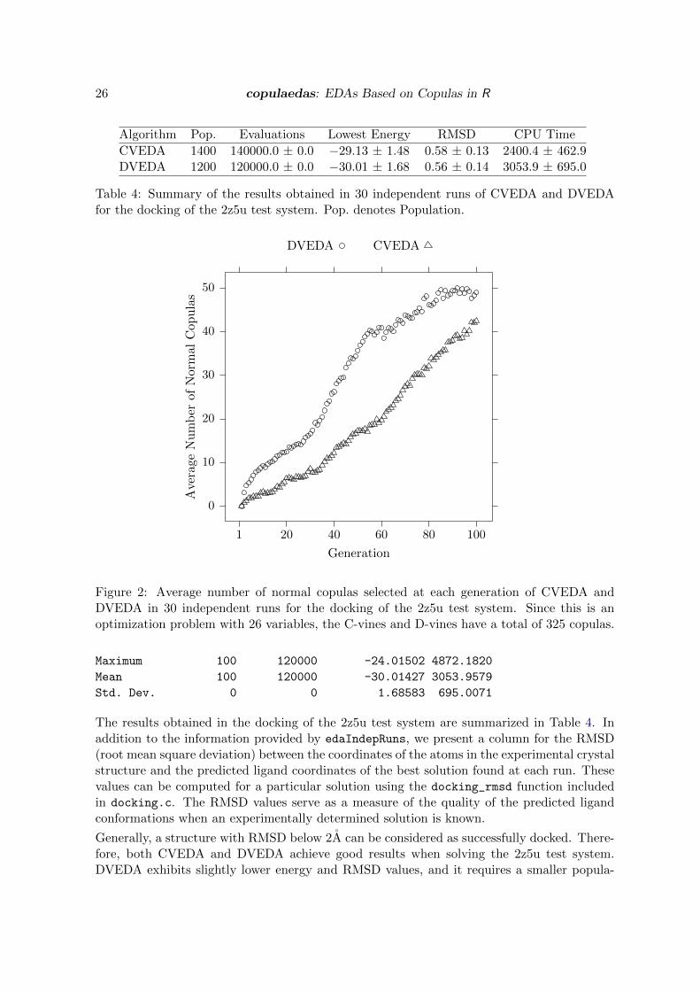
DVEDA CVEDA

Figure 2: Average number of normal copulas selected at each generation of CVEDA andDVEDA in 30 independent runs for the docking of the 2z5u test system. Since this is anoptimization problem with 26 variables, the C-vines and D-vines have a total of 325 copulas.

Maximum 100 120000 -24.01502 4872.1820

Mean 100 120000 -30.01427 3053.9579

Std. Dev. 0 0 1.68583 695.0071

The results obtained in the docking of the 2z5u test system are summarized in Table 4. Inaddition to the information provided by edaIndepRuns, we present a column for the RMSD(root mean square deviation) between the coordinates of the atoms in the experimental crystalstructure and the predicted ligand coordinates of the best solution found at each run. Thesevalues can be computed for a particular solution using the docking_rmsd function includedin docking.c. The RMSD values serve as a measure of the quality of the predicted ligandconformations when an experimentally determined solution is known.

Generally, a structure with RMSD below 2A can be considered as successfully docked. There-fore, both CVEDA and DVEDA achieve good results when solving the 2z5u test system.DVEDA exhibits slightly lower energy and RMSD values, and it requires a smaller popula-


tion size than CVEDA. On the other hand, DVEDA uses more CPU time than CVEDA, afact that might be related with more dependences being encoded in the D-vines estimatedby DVEDA than in the C-vines used by CVEDA. This situation is illustrated in Figure 2,which presents the average number of normal copulas selected by CVEDA and DVEDA ateach generation in the 30 independent runs. In both algorithms, the number of normal cop-ulas increases during the evolution, but DVEDA consistently selects more normal copulasthan CVEDA. Although the estimation procedure of the C-vines in CVEDA intends to rep-resent the strongest dependences in the first tree, the constraint that only one variable can beconnected to all the others prevent strong correlations to be explicitly encoded in the C-vines.

It is also worth noting that because of the use of the truncation procedure based on AIC inboth CVEDA and DVEDA, the number of statistical tests required to estimate the vines wasdramatically reduced. The median number of vine trees fitted in the 30 independent runs was4 in CVEDA and 5 in DVEDA out of a total of 25 trees. The interested reader is referredto Soto et al. (2012) for a deeper study of the use of EDAs based on copulas for solving themolecular docking problem.

5. Concluding remarks

We have developed copulaedas aiming at providing in a single package an open-source imple-mentation of EDAs based on copulas and utility functions to study these algorithms. In thispaper, we illustrate how to run the copula-based EDAs implemented in the package, how toimplement new algorithms, and how to perform an empirical study to compare copula-basedEDAs on benchmark functions and practical problems. We hope that these functionalitieshelp the research community to improve EDAs based on copulas by getting a better insight oftheir strengths and weaknesses, and also help practitioners to find new applications of thesealgorithms to real-world problems.

References

Aas K, Czado C, Frigessi A, Bakken H (2009). “Pair-Copula Constructions of Multiple De-pendence.” Insurance: Mathematics and Economics, 44(2), 182–198.

Abdous B, Genest C, Remillard B (2005). “Dependence Properties of Meta-Elliptical Distri-butions.” In P Duchesne, B Remillard (eds.), Statistical Modelling and Analysis for ComplexData Problems, pp. 1–15. Kluwer Academic Publisher.

Akaike H (1974). “A New Look at Statistical Model Identification.” IEEE Transactions onAutomatic Control, 19(6), 716–723.

Arderı RJ (2007). Algoritmo con estimacion de distribuciones con copula Gaussiana. Bache-lor’s thesis, University of Havana, Cuba.

Azzalini A (1981). “A Note on the Estimation of a Distribution Function and Quantiles by aKernel Method.” Biometrika, 68(1), 326–328.

Baluja S (1994). “Population-Based Incremental Learning: A Method for Integrating Ge-netic Search Based Function Optimization and Competitive Learning.” Technical Report


CMU-CS-94-163, Carnegie Mellon University, USA. URL http://www.esprockets.com/

papers/CMU-CS-94-163.ps.gz.

Barba-Moreno S (2007). Una propuesta para algoritmos de estimacion de distribucion noparametricos. Master’s thesis, Center for Research in Mathematics, Mexico.

Bedford T, Cooke RM (2001). “Probability Density Decomposition for Conditionally De-pendent Random Variables Modeled by Vines.” The Annals of Mathematics and ArtificialIntelligence, 32(1), 245–268.

Bengoetxea E, Miquelez T, Lozano JA, Larranaga P (2002). “Experimental Results in Func-tion Optimization with EDAs in Continuous Domain.” In P Larranaga, JA Lozano (eds.),Estimation of Distribution Algorithms. A New Tool for Evolutionary Computation, pp.181–194. Kluwer Academic Publisher.

Berg D, Aas K (2007). “Models for Construction of Multivariate Dependence.” NoteSAMBA/23/07, Norwegian Computing Center, NR, Norway. URL http://www.nr.no/

files/samba/bff/SAMBA2307.pdf.

Berman HM, Westbrook J, Feng Z, Gilliland G, Bhat TN, Weissig H, Shindyalov IN, BournePE (2000). “The Protein Data Bank.” Nucleic Acids Research, 28(1), 235–242.

Beyer HG, Schwefel HP (2002). “Evolution Strategies: A Comprehensive Introduction.” Nat-ural Computing, 1(1), 3–52.

Bosman PAN, Thierens D (2006). “Numerical Optimization with Real-Valued Estimation ofDistribution Algorithms.” In M Pelikan, K Sastry, E Cantu-Paz (eds.), Scalable Optimiza-tion via Probabilistic Modeling. From Algorithms to Applications, pp. 91–120. Springer-Verlag.

Brechmann EC (2010). Truncated and Simplified Regular Vines and Their Applications.Diploma thesis, University of Technology, Munich, Germany. URL http://mediatum.ub.

tum.de/doc/1079285/1079285.pdf.

Cahon S, Melab N, Talbi E (2004). “ParadisEO: A Framework for the Reusable Design ofParallel and Distributed Metaheuristics.” Journal of Heuristics, 10(3), 357–380.

Chambers J (2008). Software for Data Analysis: Programming with R. Springer-Verlag.

Cuesta-Infante A, Santana R, Hidalgo JI, Bielza C, naga PL (2010). “Bivariate Empirical andn-Variate Archimedean Copulas in Estimation of Distribution Algorithms.” In Proceedingsof the IEEE Congress on Evolutionary Computation (CEC 2010), pp. 1355–1362.

Davy M, Doucet A (2003). “Copulas: A New Insight into Positive Time-Frequency Distribu-tions.” IEEE Signal Processing Letters, 10(7), 215–218.

De Bonet JS, Isbell CL, Viola P (1997). “MIMIC: Finding Optima by Estimating ProbabilityDensities.” In M Mozer, M Jordan, T Petsche (eds.), Advances in Neural InformationProcessing Systems, volume 9, pp. 424–430. MIT Press.

Demarta S, McNeil AJ (2005). “The t Copula and Related Copulas.” International StatisticalReview, 73(1), 111–129.

http://www.esprockets.com/papers/CMU-CS-94-163.ps.gz

http://www.esprockets.com/papers/CMU-CS-94-163.ps.gz

http://www.nr.no/files/samba/bff/SAMBA2307.pdf

http://www.nr.no/files/samba/bff/SAMBA2307.pdf

http://mediatum.ub.tum.de/doc/1079285/1079285.pdf

http://mediatum.ub.tum.de/doc/1079285/1079285.pdf


Devroye L (1986). Non-Uniform Random Variate Generation. Springer-Verlag.

DOLPHIN Project Team (2012). ParadisEO 2.0.1. Inria Lille – Nord Europe, Villeneuved’Ascq, France. URL http://paradiseo.gforge.inria.fr/.

Fang HB, Fang KT, Kotz S (2002). “The Meta-Elliptical Distributions with Given Marginals.”Journal of Multivariate Analysis, 82(1), 1–16.

Gao Y (2009). “Multivariate Estimation of Distribution Algorithm with Laplace TransformArchimedean Copula.” In W Hu, X Li (eds.), Proceedings of the International Conferenceon Information Engineering and Computer Science (ICIECS 2009), pp. 1–5.

Genest C, Favre AC (2007). “Everything You Always Wanted to Know about Copula ModelingBut Were Afraid to Ask.” Journal of Hydrologic Engineering, 12(4), 347–368.

Genest C, Ghoudi K, Rivest LP (1995). “A Semiparametric Estimation Procedure of Depen-dence Parameters in Multivariate Families of Distributions.” Biometrika, 82(3), 543–552.

Genest C, Quessy JF, Remillard B (2007). “Asymptotic Local Efficiency of Cramer-von MisesTests for Multivariate Independence.” The Annals of Statistics, 35(1), 166–191.

Genest C, Remillard B (2004). “Tests of Independence or Randomness Based on the EmpiricalCopula Process.” Test, 13(2), 335–369.

Genest C, Remillard B (2008). “Validity of the Parametric Bootstrap for Goodness-of-FitTesting in Semiparametric Models.” Annales de l’Institut Henri Poincare: Probabilites etStatistiques, 44(6), 1096–1127.

Genz A, Bretz F (2009). Computation of Multivariate Normal and t Probabilities. Springer-Verlag.

Genz A, Bretz F, Miwa T, Mi X, Leisch F, Scheipl F, Hothorn T (2014). mvtnorm: Mul-tivariate Normal and t Distributions. R package version 0.9-99991, URL http://CRAN.

R-project.org/package=mvtnorm.

Gonzalez-Fernandez Y (2011). Algoritmos con estimacion de distribuciones basados en copulasy vines. Bachelor’s thesis, University of Havana, Cuba.

Gonzalez-Fernandez Y, Soto M (2014a). copulaedas: Estimation of Distribution AlgorithmsBased on Copulas. R package version 1.4.1, URL http://CRAN.R-project.org/package=

copulaedas.

Gonzalez-Fernandez Y, Soto M (2014b). vines: Multivariate Dependence Modeling withVines. R package version 1.1.0, URL http://CRAN.R-project.org/package=vines.

Haff IH, Aas K, Frigessi A (2010). “On the Simplified Pair-Copula Construction – SimplyUseful or Too Simplistic?” Journal of Multivariate Analysis, 101(5), 1296–1310.

Hauschild M, Pelikan M (2011). “An Introduction and Survey of Estimation of DistributionAlgorithms.” Swarm and Evolutionary Computation, 1(3), 111–128.

Hering C, Hofert M, Mai JF, Scherer M (2010). “Constructing Hierarchical ArchimedeanCopulas with Levy Subordinators.” Journal of Multivariate Analysis, 101(6), 1428–1433.

http://paradiseo.gforge.inria.fr/

http://CRAN.R-project.org/package=mvtnorm

http://CRAN.R-project.org/package=mvtnorm



http://CRAN.R-project.org/package=vines


Hofert M, Kojadinovic I, Maechler M, Yan J (2014). copula: Multivariate Dependence withCopulas. R package version 0.999-8, URL http://CRAN.R-project.org/package=copula.

Hooke R, Jeeves TA (1961). “Direct Search Solution of Numerical and Statistical Problems.”Journal of the Association for Computing Machinery, 8(2), 212–229.

Huey R, Morris GM, Olson AJ, Goodsell DS (2007). “A Semiempirical Free Energy Force Fieldwith Charge-Based Desolvation.” Journal of Computational Chemistry, 28(6), 1145–1152.

Hult H, Lindskog F (2002). “Multivariate Extremes, Aggregation and Dependence in EllipticalDistributions.” Advances in Applied Probability, 34(3), 587–608.

Joe H (1996). “Families of m-Variate Distributions with Given Margins and m(m − 1)/2Bivariate Dependence Parameters.” In L Ruschendorf, B Schweizer, MD Taylor (eds.),Distributions with Fixed Marginals and Related Topics, pp. 120–141.

Joe H (1997). Multivariate Models and Dependence Concepts. Chapman & Hall.

Joe H (2005). “Asymptotic Efficiency of the Two-Stage Estimation Method for the Copula-Based Models.” Journal of Multivariate Analysis, 94(2), 401–419.

Joe H, Li H, Nikoloulopoulos AK (2010). “Tail Dependence Functions and Vine Copulas.”Journal of Multivariate Analysis, 101(1), 252–270.

Joe H, Xu JJ (1996). “The Estimation Method of Inference Functions for Margins forMultivariate Models.” Technical Report 166, University of British Columbia. URLhttp://www.stat.ubc.ca/~harry/ifm.pdf.

Johnson NL, Kotz S, Balakrishnan N (1994). Continuous Univariate Distributions, volume 1.2nd edition. John Wiley & Sons.

Kennedy J, Eberhart RC (1995). “Particle Swarm Optimization.” In Proceedings of the IEEEInternational Conference on Neural Networks, volume 4, pp. 1942–1948.

Kern S, Muller SD, Hansen N, Buche D, Ocenasek J, Koumoutsakos P (2003). “LearningProbability Distributions in Continuous Evolutionary Algorithms – A Comparative Re-view.” Natural Computing, 3(1), 77–112.

Kirkpatrick S, Gelatt CD, Vecchi MP (1983). “Optimization by Simulated Annealing.” Sci-ence, 220(4598), 671–680.

Kojadinovic I, Yan J (2010). “Modeling Multivariate Distributions with Continuous MarginsUsing the copula R Package.” Journal of Statistical Software, 34(9), 1–20. URL http:

//www.jstatsoft.org/v34/i09/.

Larranaga P, Etxeberria R, Lozano JA, Pena JM (1999). “Optimization by Learning and Sim-ulation of Bayesian and Gaussian Networks.” Technical Report EHU-KZAA-IK-4/99, Uni-versity of the Basque Country. URL http://www.sc.ehu.es/ccwbayes/publications/

postscript/kzaa-ik-04-99.ps.

http://CRAN.R-project.org/package=copula

http://www.stat.ubc.ca/~harry/ifm.pdf

http://www.jstatsoft.org/v34/i09/


http://www.sc.ehu.es/ccwbayes/publications/postscript/ kzaa-ik-04-99.ps

http://www.sc.ehu.es/ccwbayes/publications/postscript/ kzaa-ik-04-99.ps


Larranaga P, Etxeberria R, Lozano JA, Pena JM (2000). “Optimization in Continuous Do-mains by Learning and Simulation of Gaussian Networks.” In Proceedings of the Workshopin Optimization by Building and Using Probabilistic Models in the Genetic and EvolutionaryComputation Conference (GECCO 2000), pp. 201–204.

Larranaga P, Lozano JA (eds.) (2002). Estimation of Distribution Algorithms: A New Tool forEvolutionary Computation, volume 2 of Genetic Algorithms and Evolutionary Computation.Kluwer Academic Publisher.

Larranaga P, Lozano JA, Bengoetxea E (2001). “Estimation of Distribution Algorithms Basedon Multivariate Normal and Gaussian Networks.” Technical Report EHU-KZAA-IK-1/01,University of the Basque Country.

Mateo JL, de la Ossa L (2006). LiO. Intelligent Systems Group and Data Mining (SIMD),Universidad de Castilla-La Mancha, Albacete, Spain. URL http://www.dsi.uclm.es/

simd/SOFTWARE/LIO/.

Mateo JL, de la Ossa L (2007). “LiO: An Easy and Flexible Library of Metaheuristics.”Technical Report DIAB-06-04-1, Department of Computing Systems, Escuela PolitecnicaSuperior de Castilla La Mancha, Albacete, Spain. URL http://www.info-ab.uclm.es/

descargas/thecnicalreports/DIAB-06-04-1/LiO.pdf.

McNeil AJ (2008). “Sampling Nested Archimedean Copulas.” Journal of Statistical Compu-tation and Simulation, 78(6), 567–581.

McNeil AJ, Neslehova (2009). “Multivariate Archimedean Copulas, d-Monotone Functionsand l1-Norm Symmetric Distributions.” The Annals of Statistics, 37(5b), 3059–3097.

Morris GM, Huey R, Lindstrom W, Sanner MF, Belew RK, Goodsell DS, Olson, J A (2009).“AutoDock4 and AutoDockTools4: Automated Docking with Selective Receptor Flexiblity.”Journal of Computational Chemistry, 30(16), 2785–2791.

Muhlenbein H, Paaß G (1996). “From Recombination of Genes to the Estimation of Distri-butions I. Binary Parameters.” In Parallel Problem Solving from Nature — PPSN IV, pp.178–187. Springer-Verlag.

Nelder JA, Mead R (1965). “A Simplex Method for Function Minimization.” ComputerJournal, 7(4), 308–313.

Nelsen RB (2006). An Introduction to Copulas. 2nd edition. Springer-Verlag.

Nocedal J, Wright SJ (1999). Numerical Optimization. Springer Series in Operations Research.Springer-Verlag.

Pelikan M (2005). Hierarchical Bayesian Optimization Algorithm. Toward a New Generationof Evolutionary Algorithms. Springer-Verlag.

Pelikan M, Goldberg DE, Lobo F (2002). “A Survey of Optimization by Building and UsingProbabilistic Models.” Computational Optimization and Applications, 21(1), 5–20.

R Core Team (2014). R: A Language and Environment for Statistical Computing. R Founda-tion for Statistical Computing, Vienna, Austria. URL http://www.R-project.org/.

http://www.dsi.uclm.es/simd/SOFTWARE/LIO/

http://www.dsi.uclm.es/simd/SOFTWARE/LIO/

http://www.info-ab.uclm.es/descargas/thecnicalreports/ DIAB-06-04-1/LiO.pdf

http://www.info-ab.uclm.es/descargas/thecnicalreports/ DIAB-06-04-1/LiO.pdf

http://www.R-project.org/


Rosenkrantz DJ, Stearns RE, Lewis, II PM (1977). “An Analysis of Several Heuristics for theTraveling Salesman Problem.” SIAM Journal on Computing, 6(3), 563–581.

Rousseeuw P, Molenberghs G (1993). “Transformation of Nonpositive Semidefinite CorrelationMatrices.” Communications in Statistics – Theory and Methods, 22(4), 965–984.

Salinas-Gutierrez R, Hernandez-Aguirre A, Villa-Diharce E (2009). “Using Copulas in Es-timation of Distribution Algorithms.” In Proceedings of the Eight Mexican InternationalConference on Artificial Intelligence (MICAI 2009), pp. 658–668.

Salinas-Gutierrez R, Hernandez-Aguirre A, Villa-Diharce E (2010). “D-Vine EDA: A NewEstimation of Distribution Algorithm Based on Regular Vines.” In Proceedings of theGenetic and Evolutionary Computation Conference (GECCO 2010), pp. 359–365.

Santana R (2011). “Estimation of Distribution Algorithms: From Available Implementationsto Potential Developments.” In Proceedings of the Genetic and Evolutionary ComputationConference (GECCO 2011), pp. 679–686.

Santana R, Bielza C, Larranaga P, Lozano JA, Echegoyen C, Mendiburu A, Armananzas R,Shakya S (2010). “Mateda-2.0: A MATLAB Package For the Implementation and Analysisof Estimation of Distribution Algorithms.” Journal of Statistical Software, 35(7), 1–30.URL http://www.jstatsoft.org/v35/i07/.

Santana R, Echegoyen C, Mendiburu A, Bielza C, Lozano JA, Larranaga P, Armananzas R,Shakya S (2009). Mateda-2.0. University of the Basque Country. URL http://www.sc.

ehu.es/ccwbayes/members/rsantana/software/matlab/MATEDA.html.

Schwarz G (1978). “Estimating the Dimension of a Model.” The Annals of Statistics, 6(2),461–464.

Silverman BW (1986). Density Estimation for Statistics and Data Analysis. Chapman andHall.

Sklar A (1959). “Fonctions de repartition a n dimensions et leurs marges.” Publications del’Institut de Statistique de l’Universite de Paris, 8, 229–231.

Soto M, Gonzalez-Fernandez Y (2010). “Vine Estimation of Distribution Algorithms.” Tech-nical Report ICIMAF 2010-561, Institute of Cybernetics, Mathematics and Physics, Cuba.

Soto M, Gonzalez-Fernandez Y, Ochoa A (2014). “Modeling with Copulas and Vines inEstimation of Distribution Algorithms.” Investigacion Operacional. Forthcoming, preprintavailable at http://arxiv.org/abs/1210.5500.

Soto M, Ochoa A, Arderı RJ (2007). “Gaussian Copula Estimation of Distribution Algorithm.”Technical Report ICIMAF 2007-406, Institute of Cybernetics, Mathematics and Physics,Cuba.

Soto M, Ochoa A, Gonzalez-Fernandez Y, Milanes Y, Alvarez A, Carrera D, Moreno E (2012).“Vine Estimation of Distribution Algorithms with Application to Molecular Docking.” InS Shakya, R Santana (eds.), Markov Networks in Evolutionary Computation, volume 14 ofAdaptation, Learning, and Optimization, pp. 209–225. Springer-Verlag.


http://www.sc.ehu.es/ccwbayes/members/rsantana/software/matlab/MATEDA.html

http://www.sc.ehu.es/ccwbayes/members/rsantana/software/matlab/MATEDA.html

http://arxiv.org/abs/1210.5500


Storn R, Price K (1997). “Differential Evolution — A Simple and Efficient Heuristic for GlobalOptimization Over Continuous Spaces.” Journal of Global Optimization, 11(4), 341–359.

The MathWorks, Inc (2014). MATLAB – The Language of Technical Computing, Ver-sion R2014a. The MathWorks, Inc., Natick, Massachusetts. URL http://www.mathworks.

com/products/matlab/.

Tierney L, Rossini AJ, Li N, Sevcikova H (2013). snow: Simple Network of Workstations. Rpackage version 0.3-13, URL http://CRAN.R-project.org/package=snow.

Trautmann H, Steuer D, Mersmann O, Bornkamp B (2014). truncnorm: Truncated Nor-mal Distribution. R package version 1.0-7, URL http://CRAN.R-project.org/package=

truncnorm.

Wang L, Zeng J, Hong Y (2009a). “Estimation of Distribution Algorithm Based onArchimedean Copulas.” In Proceedings of the First ACM/SIGEVO Summit on Geneticand Evolutionary Computation (GEC 2009), pp. 993–996.

Wang L, Zeng J, Hong Y (2009b). “Estimation of Distribution Algorithm Based on CopulaTheory.” In Proceedings of the IEEE Congress on Evolutionary Computation (CEC 2009),pp. 1057–1063.

Warren GL, Andrews CW, Capelli AM, Clarke B, LaLonde J, Lambert MH, Lindvall M,Nevins N, Semus SF, Senger S, Tedesco G, Wall ID, Woolven JM, Peishoff CE, Head MS(2006). “A Critical Assessment of Docking Programs and Scoring Functions.” Journal ofMedicinal Chemistry, 49(20), 5912–5931.

Ye B, Gao H, Wang X, Zeng J (2010). “Estimation of Distribution Algorithm Based onNested Archimedean Copulas Constructed with Levy Subordinators.” In Proceedings ofthe Eleventh International Conference on Computer-Aided Industrial Design & ConceptualDesign (CAIDCD 2010), pp. 1586–1590.

Affiliation:

Yasser Gonzalez-FernandezDepartment of Interdisciplinary MathematicsInstitute of Cybernetics, Mathematics and PhysicsCalle 15 No. 551 e/ C y D, Vedado, La Habana, CubaCurrent affiliation:School of Information TechnologyYork University4700 Keele St, Toronto, Ontario, CanadaE-mail: [email protected]

http://www.mathworks.com/products/matlab/

http://www.mathworks.com/products/matlab/

http://CRAN.R-project.org/package=snow

http://CRAN.R-project.org/package=truncnorm

http://CRAN.R-project.org/package=truncnorm

mailto:[email protected]


Marta SotoDepartment of Interdisciplinary MathematicsInstitute of Cybernetics, Mathematics and PhysicsCalle 15 No. 551 e/ C y D, Vedado, La Habana, CubaE-mail: [email protected]

Journal of Statistical Software http://www.jstatsoft.org/

published by the American Statistical Association http://www.amstat.org/

Volume 58, Issue 9 Submitted: 2012-02-17June 2014 Accepted: 2014-01-06

mailto:[email protected]

http://www.jstatsoft.org/

http://www.amstat.org/

copulaedas: an r package for estimation of distribution ... include running the edas de ned in the...

Documents